AERODYNAMIC MODEL OF THE PIPER WARRIOR II BASED ON …

AERODYNAMIC MODEL OF THE PIPER WARRIOR II BASED ON FLIGHT TEST DATA

by

Nicholas Casciola

Bachelor of Science

Aerospace Engineering

Florida Institute of Technology

2015

A thesis submitted to the College of Engineering of Florida Institute of

Technology in partial fulfillment of the requirements for the degree of

Masters of Science

in

Aerospace Engineering

Melbourne, Florida

December 2018

We the undersigned committee hereby approve the attached thesis, “Aerodynamic

Model of the Piper Warrior II Based on Flight Test Data” Nicholas Casciola.

_________________________________________________

Dr. Brian Kish, Ph.D.

Assistant Professor and Chair, Flight Test Engineering

Aerospace, Physics and Space Science

_________________________________________________

Dr. Ralph Kimberlin, Dr.-Ing.

Professor


_________________________________________________

Dr. Steven Cusick, J.D.

Associate Professor

College of Aeronautics

_________________________________________________

Dr. Daniel Batcheldor, Ph.D.

Professor and Department Head


iii

Abstract

Aerodynamic Model of the Piper Warrior II Based on Flight Test Data

By: Nicholas Casciola

Major Advisor: Brian Kish Ph.D.

Aerodynamic modeling is an important part of aircraft design and of aircraft testing.

Generally, this is done through CFD models and Wind Tunnel tests prior to the aircrafts

first flight but building the models using flight test data is also very important. It is used to

verify theoretical models generated from the computer and wind tunnel tests. They are

also useful for building simulators, particularly those in modeling and analyzing airport

traffic patterns.

These tests used a Piper Pa-28-161 Warrior II owned by the Florida Tech Flight Test

Engineering program. It has a 160hp Lycoming engine. The test pilot was Dave Schwarz

with Nicholas Casciola and Gary Greeman acting as Flight Test Engineers. The tests took

place on April 27th, 2018 East of the Orlando-Melbourne International Airport (KMLB).

The stability and control parameters were estimated using least squares, equation error,

stepwise, and output-error regression methods. These parameters were not accurately

estimated here due to several reasons. The first being the lack of a filter on several sets of

input data. The next would be that no initial heading was recorded at the start of each

maneuver; this means that yaw angle could not be found. The final piece to improve the

models is to correct for the sensor locations in the aircraft. If the sensors are not over the

cg of the aircraft, then corrections need to be made to adjust for the inertial effects of the

moment arm caused by that distance.

iv

Table of Contents

List of Figures ........................................................................................................................ vi

List of Tables ........................................................................................................................ vii

List of Symbols .................................................................................................................... viii

Acknowledgements .............................................................................................................. ix

Dedication .............................................................................................................................. x

1 Chapter 1: Introduction ................................................................................................ 1

1.1 General: ................................................................................................................. 1

1.2 Background: ........................................................................................................... 1

1.2.1 History of Aerodynamic Modelling ................................................................ 1

1.2.2 Types of Aerodynamic Modelling .................................................................. 2

1.2.3 Purpose of Aerodynamic Modelling .............................................................. 4

1.3 System Identification Theory ................................................................................. 5

1.3.1 Linear [4] ........................................................................................................ 5

1.3.2 Nonlinear [4] ................................................................................................ 11

1.3.3 Parameter Estimation and System Identification ........................................ 12

2 Chapter 2: Test Methods ............................................................................................. 15

2.1 Test Item Description ........................................................................................... 15

2.2 Test Objectives ..................................................................................................... 16

2.3 Limitations and Constraints ................................................................................. 16

2.4 Test Procedure ..................................................................................................... 16

2.4.1 Longitudinal column impulse and doublet .................................................. 21

2.4.2 Lateral Directional Inputs: Wheel and Pedal Impulse and Doublets ........... 21

2.4.3 All Axes Control Doublet .............................................................................. 22

2.4.4 Static Longitudinal Stability ......................................................................... 22

2.4.5 Static Lateral-Directional Stability, Steady Heading Sideslip ....................... 23

2.5 Data Reduction Procedure ................................................................................... 23

3 Chapter 3: Results ........................................................................................................ 26

4 Conclusion.................................................................................................................... 47

v

4.1 Conclusion............................................................................................................ 47

4.2 Future Work ......................................................................................................... 47

5 References ................................................................................................................... 49

6 Appendices .................................................................................................................. 50

6.1 Appendix A: SIDPAC MatLab Codes ..................................................................... 50

6.1.1 deriv.m ......................................................................................................... 50

6.1.2 smoo.m ........................................................................................................ 51

6.1.3 compfc.m and compmc.m ........................................................................... 55

6.1.4 xsmep.m....................................................................................................... 60

6.1.5 lesq.m........................................................................................................... 62

6.1.6 r_colores.m .................................................................................................. 66

6.1.7 model_disp.m .............................................................................................. 68

6.1.8 swr.m ........................................................................................................... 73

6.1.9 nldyn_psel.m................................................................................................ 81

6.1.10 oe.m ............................................................................................................. 86

6.1.11 nldyn.m ........................................................................................................ 96

6.1.12 m_colores.m ................................................................................................ 99

6.1.13 plotpest.m .................................................................................................. 102

vi

List of Figures

Figure 1: Test range and home airport for the Flight Test of the Piper Warrior II .............. 17

Figure 2: Flight Test Data for 5000 ft Column Doublet ........................................................ 27

Figure 3: Flight Test Data Z-force and Pitching Moment Non-Dimensional Coefficients .... 28

Figure 4: Regressors for the Equation-Error Parameter Estimation .................................... 29

Figure 5: Equation-Error Parameter Estimation Results...................................................... 30

Figure 6: Pitching moment Coefficient Model plotted over flight data .............................. 32

Figure 7: Ouput-Error Time Domain Modeling Flight Data ................................................. 33

Figure 8: Output-Error Parameter Estimation Model vs. Flight Data .................................. 34

Figure 9: Lateral Flight Test Data ......................................................................................... 36

Figure 10: Y-force and Rolling moment coefficients for Lateral Maneuver ........................ 37

Figure 11: Equation Error Regressors for Lateral Model ..................................................... 38

Figure 12:Y-Force Equation-Error Parameter Estimation Model ........................................ 39

Figure 13: Rolling Moment Model using Step-Wise Regression ......................................... 41

Figure 14: Yawing Moment Coefficient Equation-Error Model ........................................... 43

Figure 15: Output-Error Modelling Flight Data .................................................................... 44

Figure 16: Output-Error Parameter Estimation Model ....................................................... 45

vii

List of Tables

Table 1: Test Aircraft Information [2] [3] ............................................................................. 15

Table 2: Test Configurations ................................................................................................ 18

Table 3: Z-Force parameter estimation ............................................................................... 29

Table 4: Step-Wise Regression for the Pitching Moment coefficient .................................. 31

Table 5: Pitching moment estimated parameters ............................................................... 32

Table 6: Parameter Estimation Results ................................................................................ 35

Table 7: Y-Force Parameter Estimation ............................................................................... 39

Table 8: Step-Wise Regression for Rolling Moment Lateral Maneuver .............................. 40

Table 9: Rolling Moment Parameter Estimation Results ..................................................... 41

Table 10: Step-Wise Regression for Yawing Moment Lateral Maneuver ............................ 42

Table 11: Yawing Moment Parameter Estimation Results .................................................. 43

Table 12: Lateral Parameter Estimation Results .................................................................. 46

viii

List of Symbols

CZa-Z-force coefficient due to angle of attack (alpha)

CZq-Z-force coefficient due to pitch rate

CZde-Z-force coefficient due to elevator deflection

CZo-initial Z-force coefficient

Cma-Moment coefficient due to angle of attack

Cmq- Moment coefficient due to pitch rate

Cmde- Moment coefficient due to elevator deflection

Cmo-initial moment coefficient

Azo-acceleration in the z-axis

CYb-Y-force coefficient due to angle of sideslip (beta)

CYp-Y-force coefficient due to roll rate

CYdr-Y-force coefficient due to rudder deflection

CYda-Y-force coefficient due to aileron deflection

CYo-initial Y-force coefficient

Crb-Rolling moment coefficient due to sideslip angle

Crp-Rolling moment coefficient due to roll rate

Crdr-Rolling moment coefficient due to rudder deflection

Crda-Rolling moment coefficient due to aileron deflection

Cro-initial Rolling moment coefficient

Cnb-Yawing moment coefficient due to sideslip angle

Cnp-Yawing moment coefficient due to roll rate

Cndr-Yawing moment coefficient due to rudder deflection

Cnbr-Yawing moment coefficient due to beta*rudder deflection cross term

Cno-initial Yawing moment coefficient

Ayo-acceleration in the y-axis

ix

Acknowledgements

I would like to thank Dr. Brian Kish for all his support and assistance during this thesis.

When new data had to be gathered after the first attempt had failed he graciously helped

gather the new data. He consistently provided encouragement and guidance throughout

my graduate career and was never opposed to new or strange ideas and was always

willing to work with me to make sure that I got out of my time here what I wanted.

I would also like to thank Dr. Ralph Kimberlin for serving on my thesis committee. His

leadership and instruction led to being able to do this thesis. The passion and skill he

shows for aviation are apparent in everything he does.

Dr. Steven Cusick is another that I would like to thank, he kindly agreed to be member of

my thesis committee and is a very welcome member.

None of the data seen here would have been there if it wasn’t for Dr. Isaac Silver. He set

up the data recorders and program the Garmin to provide output through the Stratus.

Without him none of the calculations would have been possible.

Finally, I would like to thank Gary Greenman from Gulfstream. He was also working on his

thesis trying to find the aerodynamic model for the Warrior and his assistance in figuring

out what we were doing in terms of how SIDPAC worked, setting up test cards, and

finding Eugene Morelli’s textbook has been invaluable. Without his help this thesis never

would have been finished.

x

Dedication

I would like to dedicate this thesis to all those who helped and supported me along the

way. My parents who have encouraged me since I was little.

I also want to dedicate this to my girlfriend Emily, she has been instrumental in the

accomplishment of this thesis. She has always been there to help and support and lend a

critical eye to my writing.

1

1 Chapter 1:

Introduction

1.1 General:

These tests are to find the aerodynamic models for the Piper PA-28-161 Warrior II

through the use of flight tests and the SIDPAC MATLAB files, System IDentification

Programs for AirCraft. Dave Schwarz was the test pilot for this test and Gary Greenman

and Nicholas Casciola were the test engineers who built the aerodynamic models.

Testing was requested by the Flight Test Engineering department at Florida

Institute of Technology. The testing was for academic purposes and was performed within

the guidelines and restrictions of the Pilots Operating Handbook for the Piper PA-28-161.

1.2 Background:

1.2.1 History of Aerodynamic Modelling

When aircraft were first being built and developed there was a limited

understanding of aerodynamics and only the most basic aerodynamic properties could be

found. William F. Milliken Jr. created one of the first approaches for aerodynamic

modelling, using frequency response and simple graphical methods to analyze flight data

and obtain static and dynamic parameters in 1947. In 1951 Harry Greenberg and Marvin

Shinbrot created a better, more general and rigorous approach to find aerodynamic

parameters by using transient maneuvers which were based on ordinary and nonlinear

least squares methods. When more modern computer systems became available in the

60s and 70s incredible strides in modeling techniques occurred and a new field was born;

system identification. Conferences and symposiums began to be held based around this

discipline of system identification. The proceedings from the IFAC Symposia on

Identification and System Parameter Estimation and the survey paper by K. J. Anström

2

and P. Eykhoff are excellent sources of general system identification information. The first

of the Symposiums was held in 1967 and have continued every three years since then.

Many new approaches for the development and application of estimation techniques also

came about with the advent of better computer systems. Some of the most substantial

contributions came from Taylor, L. W., Iliff, K. W., Powers, B. G., Mehra, R. K., Stepner, D.

E., and O. H. Gerlach all contributed to papers that provided theses new approaches.

Taylor, Iliff, and Powers worked together on one such paper and Mehra and Stepner on

another. Mehra also wrote one individually as did Gerlach. More complicated challenges

started to arise as highly maneuverable and unstable aircraft began to appear, but many

people addressed these challenges and helped create solutions for the difficulties that

had formed. Based on the work of these people and many others it is possible to

determine the mathematical structure of; and estimate the parameters of the

aerodynamic models [4].

1.2.2 Types of Aerodynamic Modelling

There are many ways to perform aerodynamic modelling of aircraft. It can be

accomplished through flying a full-size aircraft and collecting flight data, building a small-

scale model and using a wind tunnel to gather the data, or using Computational Fluid

Dynamics to generate a model through computer code.

Currently one of the most common is to use Computational Fluid Dynamic

methods otherwise known as CFD. Using CFD methods means that the models can be

generated before the aircraft is even built. Using CFD codes means that the aircraft does

not need to be built and the aerodynamic coefficients can be found for a wide variety of

flight regimes and use cases without the complexity of a wind tunnel or needing to build a

full-size aircraft. Downsides to CFD methods are that they require a good grasp of the

software being used which can require extra training, the models can be difficult to

accurately build, especially with unusual configurations, powerful computers need to be

used, and finally even the best CFD code can’t accurately model the nonlinearities of real

3

world flight. Altogether this means that while CFD models may be a good first step,

further aerodynamic modeling is needed to confirm the computer models and fill in the

edges of the flight envelope [10].

Wind tunnels are another common method of calculating aerodynamic models.

Using data gathered through wind tunnel runs and similar calculation methods as done

with full size flight models the aerodynamic model of the aircraft can be found. This is a

common method since it gives accurate data on many real-world situations.

Unfortunately, this method does require a wind tunnel which can be very large and quite

costly as well as a physical aircraft model. Wind tunnels also run into an issue with scale,

unless a full-size wind tunnel, such as the National Full-Scale Aerodynamics Complex at

NASA Ames, is used [7]. The force and moment calculations need to be corrected for wind

tunnel use and real-world speed. Density measures may be inaccurate because of this [1].

Another issue is mounting of the model in the wind tunnel. Unfortunately, the mount

needs to be considered as it affects the flow around the model a great deal. This is not an

easy accomplishment and can also lead to issues with the testing [6].

In the end, the most accurate way to find aerodynamic models of an aircraft is

build and fly it at full size, a process often known as aircraft system identification. This

does have a few drawbacks. Cost of the full scale aircraft flight tests and danger to the

pilots as well as those on the ground are the biggest ones, but this is still a very important

process to use. Benefits of these system identification methods are that they can be

performed with the rest of the flight testing of a new aircraft. In fact, many of the

maneuvers used in flight testing are the same needed to gather the data for system

identification. Use of a full-size aircraft in flight reduces the uncertainties due to the

supports or scale sizes from the wind tunnel. Nonlinearities being found and analyzed as

part of the data from wind gusts or other nonlinear portions of flight reality unlike in the

CFD case. Finally, using flight test methods to build aerodynamic models is also useful

because you can use it to build the model for an aircraft that never had one calculated

4

when it was designed. Which can help with future modifications to the aircraft or the

design of new aircraft that borrow main components. In general, the most complete set

of flight models can be built from flight test data for current or future aircraft, although

since the methods introduce further costs and risks either CFD or wind tunnel models

should be used prior to flight tests to ensure the aircraft can fly safely. In this case then,

aircraft system identification instead takes the purpose of verifying the models developed

using other methods.

1.2.3 Purpose of Aerodynamic Modelling

Aerodynamic modelling is a common part of most modern aircraft design. It allows

for the flight characteristics of a new aircraft to be analyzed prior to test flying keeping

early flights safer for the test pilots. It is also important for simulation purposes to train

new pilots and teach experienced pilots to safely fly new aircraft. All of this, though,

seems like it would only be useful to new aircraft and not to those that have been flying

for years, meaning that finding aerodynamic models through flight test methods is

unnecessary since the use of models are generally just for pre-flight analysis. Nothing

could be further from the truth though. In reality, aerodynamic modeling through flight

test methods have huge amounts of uses. It allows verification of CFD and wind tunnel

models, which can confirm or deny the theoretical performance and controllability of the

aircraft which is an important step before producing new aircraft for the market. This still

doesn’t explain why the aerodynamic model of an aircraft that has been built, sold, and

flown for almost 50 years is needed or useful since simulators can be analyzed for feel by

pilots who have hundreds to thousands of hours flying the aircraft. The use of analyzing

the aerodynamic models of an aircraft as old as the Piper Warrior II is that the models can

be fed into simulators for uses such as analyzing airport traffic patterns to account for

vortices, both that the aircraft may run into and those that it may produce. This

knowledge can help the optimization of airport traffic patterns and safety tolerances

involving the aircraft analyzed [3].

5

1.3 System Identification Theory

The basis of system identification theory is to build mathematical models that will

represent the predicted output from a set of inputs. For aircraft system theory, the inputs

represent control inputs from the pilot, while the outputs are how the aircraft responds in

terms of roll, pitch, and yaw. This means that with an accurate mathematical model for an

aircraft the result of any control movement can be accurately predicted, and pilots can be

prepared for what the aircraft will do.

These mathematical models tend to take the form of a set of differential equations

that relate the input to the output, as per the basis of what system identification is.

Generally, the inputs can be preset by the experimenter, which means that the outputs

must be measured. In the case of aircraft flight models the inputs need to be measured as

well due to the potential variability of input from the pilot. The output at any given time

should be a function of the input and current aircraft state and flying conditions. These

mathematical models can be designated as either linear or non-linear [4].

1.3.1 Linear [4]

A linear model is expressed as seen in Equation 1 and Equation 2 below. In these

models A, B, C, and D are all matrices representing different things. A represents the

stability or system matrix, B is the control or input matrix, while C and D are

transformation matrices for the outputs and x0 is the vector of initial conditions for the

system. The four matrices are all constants for a system. That is, they do not vary with

time.

EQUATION 1: �̇�(𝒕) = 𝑨𝒙(𝒕) + 𝑩𝒖(𝒕) 𝒙(𝟎) = 𝒙𝟎

EQUATION 2: 𝒚(𝒕) = 𝑪𝒙(𝒕) + 𝑫𝒖(𝒕)

These equations are then solved as any differential equations are solved, first a

homogenous solution is found by solving the system for a zero-input case through the

6

separation of variables. Then the homogenous form of the vector equation gets solved

through the infinite series in Equation 5. Equation 3 and Equation 4 show the

homogenous form of Equation 1 and the proposed solution respectively.

EQUATION 3: �̇�(𝒕) = 𝑨𝒙(𝒕) 𝒙(𝟎) = 𝒙𝟎

EQUATION 4: 𝒙(𝒕) = 𝒆𝑨𝒕𝒙𝟎

EQUATION 5: 𝒆𝑨𝒕 = 𝑰 + 𝑨𝒕 +𝑨𝟐𝒕𝟐

𝟐!+

𝑨𝟑𝒕𝟑

𝟑!+ ⋯

Solving these gives the linear model of the system under consideration. This is

done through knowing the time derivative of eAt which can be seen in Equation 6.

EQUATION 6:𝒅

𝒅𝒕𝒆𝑨𝒕 = 𝑨 + 𝑨𝟐𝒕 +

𝑨𝟑𝒕𝟐

𝟐!+ ⋯ = 𝑨𝒆𝑨𝒕

Therefore, the proposed solution in Equation 4 satisfies the homogenous

equation since at t=0, 𝑥(0) = 𝑥0. The linear model in Equation 1 has a forcing function

𝑩𝒖(𝑡) which can be thought of as a series of impulses and the response can be found

from the convolution integral shown in Equation 7.

EQUATION 7: 𝒙(𝒕) = 𝒆𝑨𝒕𝒙𝟎 + ∫ 𝒆𝑨(𝒕−𝝉)𝑩𝒖(𝝉)𝒅𝝉𝒕

𝟎

The part of Equation 7 to the right of the equals sign is the free response to initial

conditions and the forced response to the input 𝑢(𝑡). The first term is the free response

and the second term is the forced response. If Equation 7 gets substituted into Equation 2

then the result is Equation 8.

EQUATION 8: 𝒚(𝒕) = 𝑪 [𝒆𝑨𝒕𝒙𝟎 + ∫ 𝒆𝑨(𝒕−𝝉)𝑩𝒖(𝝉)𝒅𝝉𝒕

𝟎] + 𝑫𝒖(𝒕)

The next step is to define a new matrix using the Dirac delta function, Equation 9,

as 𝑮(𝑡) seen in Equation 10.

EQUATION 9: 𝜹(𝒕) = {𝟎 𝒇𝒐𝒓 𝒕 ≠ 𝟎∞ 𝒇𝒐𝒓 𝒕 = 𝟎

𝒂𝒏𝒅 ∫ 𝜹(𝒕)𝒅𝒕 = 𝟏∞

−∞

7

EQUATION 10: 𝑮(𝒕) = 𝑪𝒆𝑨𝒕𝑩 + 𝑫𝜹(𝒕)

Then, combining Equation 9 and Equation 10 gives

EQUATION 11: 𝒚(𝒕) = 𝑪𝒆𝑨𝒕𝒙𝟎 + ∫ 𝑮(𝒕 − 𝝉)𝒖(𝝉)𝒅𝝉𝒕

𝟎

Here 𝑮(𝑡) is the weighting function matrix. When this is solved over a very small

time step the input vector can be considered constant and the result is seen in Equation

12 below where 𝑥(𝑖) = 𝑥(𝑖Δ𝑡)

EQUATION 12: 𝒙(𝒊) = 𝒆𝑨𝚫𝒕𝒙(𝒊 − 𝟏) + [𝑨−𝟏(𝒆𝑨𝚫𝒕 − 𝑰)]𝑩𝒖(𝒊 − 𝟏)

If the homogenous differential equation, Equation 3, is returned to the potential

solution is

EQUATION 13: 𝒙(𝒕) = 𝝃𝒆𝝀𝒕

With 𝜆 being a scalar and 𝜉 being a vector. This can then be substituted into

Equation 3 and the result is seen below in Equation 14 and Equation 15.

EQUATION 14: 𝝀𝝃𝒆𝝀𝒕 = 𝑨𝝃𝒆𝝀𝒕

EQUATION 15: (𝝀𝑰 − 𝑨)𝝃 = 𝟎

Then, as long as the determinant of the coefficient matrix is equal to zero then

there exists a nonzero solution to these equations. That is as long as Equation 16 holds

than there is a non-trivial solution to the above equation sets.

EQUATION 16: |𝝀𝑰 − 𝑨| = 𝟎

The roots of Equation 16 are the eigenvalues for the system and if they are

distinct then they each have an eigenvector that corresponds to the respective

eigenvalue. The eigenvalues for these solutions can either be real or imaginary and the

solution that corresponds to each real eigenvalue or each pair of imaginary eigenvalues is

8

known as a mode and the solution to the homogeneous equation is a sum of the modal

components.

EQUATION 17: 𝒙(𝒕) = 𝒄𝟏𝝃𝟏𝒆𝝀𝟏𝒕 + 𝒄𝟐𝝃𝟐𝒆𝝀𝟐𝒕 + ⋯ + 𝒄𝒏𝒔𝝃𝒏𝒔

𝒆𝝀𝒏𝒔𝒕

In Equation 17 the scalars 𝑐𝑖, 𝑖 = 1,2, … , 𝑛𝑠 are determined by the initial condition

from Equation 3, 𝒙(0) = 𝒙𝟎.

Now, if the forcing function is a sequence of impulses like earlier, then the

solution for the forcing function inside the convolution integral follows a similar analysis

to what was just performed. This means that the participation of each mode depends on

how the forcing function is projected along the eigenvectors.

If the Laplace transform is applied to Equation 1 and Equation 2 then the results

are

EQUATION 18: 𝒔�̃�(𝒔) = 𝑨�̃�(𝒔) + 𝑩�̃�(𝒔)

and

EQUATION 19: �̃�(𝒔) = 𝑪�̃�(𝒔) + 𝑫�̃�(𝒔)

In these equations the variable s is complex and then the transformed state is seen in

Equation 20 below.

EQUATION 20: �̃�(𝒔) = ∫ 𝒙(𝒕)∞

𝟎𝒆−𝒔𝒕𝒅𝒕

This is the same for �̃�(𝑠) and �̃�(𝑠). Then the result is Equation 21 below.

EQUATION 21: �̃�(𝒔) = [𝑪(𝒔𝑰 − 𝑨)−𝟏𝑩 + 𝑫]�̃�(𝒔) = 𝑮(𝒔)�̃�(𝒔)

In Equation 21 the matrix 𝑮(𝑠) is a transfer function matrix where the elements are

EQUATION 22: [𝑮𝒋𝒌] =𝒏𝒖𝒎𝒋𝒌(𝒔)

𝒅𝒆𝒏(𝒔) 𝒇𝒐𝒓 {

𝒋 = 𝟏, 𝟐, … , 𝒏𝒐

𝒌 = 𝟏, 𝟐, … , 𝒏𝒊

9

and 𝑛𝑜 and 𝑛𝑖 are the number of outputs, while 𝑛𝑢𝑚𝑗𝑘(𝑠) and 𝑑𝑒𝑛(𝑠) are polynomials in

s. The denominator polynomial, 𝑑𝑒𝑛(𝑠), is the characteristic polynomial and 𝑛𝑢𝑚𝑗𝑘(𝑠),

the numerator, corresponds to the transfer function that is the jth output to the kth

input. If s is set to 𝑠 = 𝑗𝜔 where 𝑗 = √−1 and 𝜔 is angular frequency, then instead of the

Laplace transform, it becomes the Fourier transform as seen in Equation 23 and Equation

24 below.

EQUATION 23: �̃�(𝒋𝝎) = ∫ 𝒚(𝒕)∞

𝟎𝒆−𝒋𝝎𝒕𝒅𝒕

EQUATION 24: �̃�(𝒋𝝎) = ∫ 𝒖(𝒕)∞

𝟎𝒆−𝒋𝝎𝒕𝒅𝒕

Then the transfer function matrix instead becomes the frequency response matrix

𝑮(𝑗𝜔) which can be determined experimentally. The elements of the matrices 𝑨, 𝑩, 𝑪,

and 𝑫 from Equation 1 and Equation 2 are model parameters that remain constant. This

means that they do not depend on the time, the input, their derivatives, or the current

state. Although, theses matrix parameters can depend on time, that changes Equation 1

and Equation 2 to instead become Equation 25 and Equation 26 below.

EQUATION 25: �̇�(𝒕) = 𝑨(𝒕)𝒙(𝒕) + 𝑩(𝒕)𝒖(𝒕) 𝒙(𝒕𝟎) = 𝒙𝟎

EQUATION 26: 𝒚(𝒕) = 𝑪(𝒕)𝒙(𝒕) + 𝑫(𝒕)𝒖(𝒕)

Which represent a time varying system rather than the time-invariant system

previously discussed. Here the solution is seen in Equation 27, where Φ is the state

transition matrix and is a function of both the time of the input 𝜏 and the time of the

result t.

EQUATION 27: 𝒚(𝒕) = 𝑪(𝒕)𝚽(𝒕, 𝒕𝟎)𝒙(𝒕𝟎) + ∫ 𝑪(𝒕)𝚽(𝒕, 𝛕)𝐁(𝛕)𝒖(𝝉)𝒅𝝉 + 𝑫(𝒕)𝒖(𝒕)𝒕

𝒕𝟎

If uncertain disturbances are added to the input and Equation 25 then rather than a

deterministic model, the system becomes a stochastic one. This means that the inherent

randomness that exists in any real-world system is accounted for and that the same set of

10

parameters and initial conditions can lead to different results. This changes Equation 25

and Equation 26 to Equation 28 and Equation 29 and the vector 𝒘(𝑡) is process noise,

while 𝑩𝑤(𝑡) is the control matrix for the vector 𝒘(𝑡).

EQUATION 28: �̇�(𝒕) = 𝑨(𝒕)𝒙(𝒕) + 𝑩𝒘(𝒕)𝒘(𝒕) 𝒙(𝒕𝟎) = 𝒙𝟎

EQUATION 29: 𝒚(𝒕) = 𝑪(𝒕)𝒙(𝒕) + 𝑫(𝒕)𝒖(𝒕)

Because 𝒘(𝑡) is generally assumed to be white noise identified by its mean and

covariance matrices as seen below.

EQUATION 30: 𝑬[𝒘(𝒕)] = 𝟎

EQUATION 31: 𝑬[𝒘(𝒕𝒊)𝒘𝑻(𝒕𝒋)] = 𝑸(𝒕𝒊)𝜹(𝒕𝒊 − 𝒕𝒋)

In Equation 30 and Equation 31 while 𝛿(𝑡𝑖 − 𝑡𝑗) is the dirac delta function, 𝐸[ ] is the

expectation operator. The expectation operator gives the expected value or mean of a

random variable X, that is

EQUATION 32: 𝑬(𝑿) = ∫ 𝒙𝒑(𝒙)𝒅𝒙∞

−∞

And 𝑝(𝑥) is the probability density function for X. To finish modeling this stochastic

system the vector of initial conditions needs to be declared as does the affiliation

between 𝒙(𝑡0) and 𝒘(𝑡) generally specified as

EQUATION 33: 𝑬[𝒙(𝒕𝟎)] = �̅�𝟎

EQUATION 34: 𝑬{[𝒙(𝒕𝟎) − �̅�𝟎][𝒙(𝒕𝟎) − �̅�𝟎]𝑻} = 𝑷𝟎

EQUATION 35: 𝑬[𝒙(𝒕𝟎)𝒘𝑻(𝒕)] = 𝟎

With 𝑷0 being a 𝑛𝑠 𝑥 𝑛𝑠 constant error covariance matrix. In the above equations �̅�0 is

used since the initial condition is the expected value of 𝒙(𝑡0), the stochastic quantity.

Because a problem arises if the continuous-time formulation for the stochastic system

used with 𝒘(𝑡), due to 𝒘(𝑡) being a zero-mean random vector for a fixed length of time.

11

In order to avoid this the model should be formed as a discrete time model. That is the

signals would be sampled at 𝑡0 + 𝑖Δ𝑡, 1, 2, …, with Δ𝑡 between samples being constant,

then

EQUATION 36: 𝒙(𝒊) ≡ 𝒙(𝒕𝟎 + 𝒊𝚫𝒕) 𝒊 = 𝟎, 𝟏, 𝟐, …

Then 𝒖(𝑖) and 𝒘(𝑖) are similarly for the discrete-time state-space stochastic model given

by Equation 37 and Equation 38.

EQUATION 37: 𝒙(𝒊) = 𝚽(𝒊 − 𝟏)𝒙(𝒊 − 𝟏) + 𝚪 (𝒊 − 𝟏)𝒖(𝒊 − 𝟏) + 𝚪𝒘(𝒊 − 𝟏)𝒘(𝒊 − 𝟏)

EQUATION 38: 𝒚(𝒊) = 𝑪(𝒊)𝒙(𝒊) + 𝑫(𝒊)𝒖(𝒊) 𝒊 = 𝟏, 𝟐, …

1.3.2 Nonlinear [4]

These prior mathematical concepts are great for linear situations; that is, where

there is a linear relationship between the input and output. Unfortunately though, the

real-world is rarely linear. When only restricted conditions are used, then the linear

models can predict nonlinear responses quite well, but when that type of approximation

isn’t possible then a nonlinear model must be used instead. In the same stochastic, time-

varying system used previously the new model equations can be seen below.

EQUATION 39: �̇�(𝒕) = 𝒇[𝒙(𝒕), 𝒖(𝒕), 𝒘(𝒕), 𝒕] 𝒙(𝟎) = 𝒙𝟎

EQUATION 40: 𝒚(𝒕) = 𝒉[𝒙(𝒕), 𝒖(𝒕)]

Because these equations are nonlinear, numerical methods such as the fourth-

order Runge-Kutta must be used, as with nonlinear systems in general. A common

nonparametric representation of these nonlinear systems is the Volterra series. The

Volterra series can be seen in Equation 41 below

EQUATION 41: 𝒚(𝒕) = ∑ 𝒚𝒏(𝒕)∞𝒏=𝟏

And 𝑦𝑛(𝑡) is defined as

12

EQUATION 42: 𝒚𝟏(𝒕) = ∫ 𝒈𝟏(𝝉𝟏)𝒖(𝒕 − 𝝉𝟏)𝒅𝝉𝟏𝒕

𝟎

EQUATION 43: 𝒚𝟐(𝒕) = ∫ ∫ 𝒈𝟐(𝝉𝟏, 𝝉𝟐)𝒖(𝒕 − 𝝉𝟏)𝒖(𝒕 − 𝝉𝟐)𝒅𝝉𝟏𝒅𝝉𝟐𝒕

𝟎

𝒕

𝟎

EQUATION 44: 𝒚𝒏(𝒕) = ∫ ∫ … ∫ 𝒈𝒏(𝝉𝟏, 𝝉𝟐, … , 𝝉𝒏)𝒖(𝒕 − 𝝉𝟏) … 𝒖(𝒕 − 𝝉𝒏)𝒅𝝉𝟏 … 𝒅𝝉𝒏𝒕

𝟎

𝒕

𝟎

𝒕

𝟎

And the 𝑔1(𝜏1), 𝑔2(𝜏1, 𝜏2), … , 𝑔𝑛(𝜏1, 𝜏2, … , 𝜏𝑛) terms are the impulse responses. This

means that the Volterra series description of the system is a generalization of the linear

model through a convolution integral.

1.3.3 Parameter Estimation and System Identification

System identification is generally started by performing an experiment with

inputs specified using theoretical knowledge about the system and the purpose of the

identification. The model class is also specified using that same theoretical knowledge as

well as from experimental data. The equivalence of the model and physical system is

commonly expressed through a scalar cost function which quantifies the relationship

between the physical system output, z, and the model output, y.

EQUATION 45: 𝑱 = 𝑱(𝒛, 𝒚)

And 𝐽 usually consists of a weighted sum of squared differences. The relation

between 𝑧 and 𝑦 are then expressed through a measurement equation, as seen in

Equation 46. Here v is the measurement error or measurement noise and is assumed to

be random.

EQUATION 46: 𝒛 = 𝒚 + 𝒗

This noise unfortunately cannot be measured directly but may be assumed or

estimated using smoothing and filtering techniques. Since finding the best model based

off of Equation 45 may lead to the consideration of far too many models, instead system

identification becomes an optimization problem to find a model 𝑀 from a class of models

that minimizes the cost function 𝐽. These models may often be limited to models that

13

have the same mathematical structure, 𝑀∗, but different parameters in the model, 𝜽.

That is

EQUATION 47: 𝑴∗ = {𝑴(𝜽)}

Then data that is collected when running the experiment is

EQUATION 48: 𝒁𝑵 = [𝒛(𝟏), 𝒖(𝟏), 𝒛(𝟐), 𝒖(𝟐), … , 𝒛(𝑵), 𝒖(𝑵)]

And N is the number of data points. After the structure of the model is chosen, system

identification is just the selection of a value for 𝜽, from the data in 𝒁𝑁 that minimizes 𝐽.

EQUATION 49: 𝑱 = 𝑱[𝒁𝑵, 𝒀𝑵(𝜽)]

With 𝒀𝑁(𝜽) being the model outputs depending on the vector 𝜽. Therefore, system

identification is as simple as model parameter estimation. This allows the exploitation of

statistical interference methods, primarily estimation theory. The results from this

process will include the parameter estimates, error bounds, and information used to test

statistical hypothesis.

When this method is applied to aircraft the dynamic equations of motion for

aircraft need to be used. Those equations are a combination of the aircraft mass 𝑚, the

inertia tensor 𝑰, Euler angles 𝜻 which is the attitude of the aircraft relative to the earth

axes, the translational and angular velocity vectors, 𝑽 and 𝝎 respectively, for the aircraft

motion, and the control vector 𝒖. The physical forces from gravity, thrust, and

aerodynamic forces, 𝑭𝐺 , 𝑭𝑇 , and 𝑭𝐴 respectively, as well as 𝑴𝐴, the aerodynamic

moments, and 𝑴𝑇, moment due to the thrust, are also included in the equation. To

include gravitational force kinematic differential equations are added to describe the

attitude of the aircraft in reference to earth axes as can be seen in Equation 50 and

Equation 51 below. Since thrust forces and moments are generally found through static

ground tests and through installation geometry, system identification for aircraft is then

14

simplified to the calculation of the model structure for the aerodynamic forces and

moments, and the estimation of parameters in those structures using the measured data.

EQUATION 50: 𝒎�̇� + 𝝎 ∗ 𝒎𝑽 = 𝑭𝑮(𝜻) + 𝑭𝑻 + 𝑭𝑨(𝑽, 𝝎, 𝒖, 𝜽)

EQUATION 51: 𝑰�̇� + 𝝎 ∗ 𝑰𝝎 = 𝑴𝑻 + 𝑴𝑨(𝑽, 𝝎, 𝒖, 𝜽)

Then, when Equation 50 and Equation 51 have the output equations added to

connect the aircraft state and controls to the measured outputs you get,

EQUATION 52: �̇�(𝒕) = 𝒇[𝒙(𝒕), 𝒖(𝒕), 𝜽] 𝒙(𝟎) = 𝒙𝟎

EQUATION 53: 𝒚(𝒕) = 𝒉[𝒙(𝒕), 𝒖(𝒕), 𝜽]

EQUATION 54: 𝒛(𝒊) = 𝒚(𝒊) + 𝒗(𝒊) 𝒊 = 𝟏, 𝟐, … , 𝑵

Here 𝒙 has the components of 𝑽, 𝝎, and 𝜻. The output vector 𝒚(𝑡) consists of aircraft

response variables and usually includes state variables. The discrete measured outputs in

𝑧(𝑖) are tampered by the measurement noise 𝒗(𝑖) as discussed in Equation 46 [4].

15

2 Chapter 2:

Test Methods

2.1 Test Item Description

The Florida Institute of Technology Flight Test Engineering Piper PA-28-161 Warrior

II was the aircraft being tested. It is a low-wing, single engine, 4-seat aircraft with a

maximum gross take-off weight of 2440 lbs. The engine is a 160 HP Lycoming O-320

engine. It has a reversible control system; that is, the controls move the control surfaces

and the control surfaces in turn move the controls. Table 1 lists more details about the

Piper PA-28-161 Warrior II.

TABLE 1: TEST AIRCRAFT INFORMATION [8][9]

Aircraft

Manufacturer Piper Aircraft Inc.

Model PA-28-161 Warrior II

Registration Number N618FT

Max Take-off Weight 2440 lbs.

Empty Weight 1568.5 lbs.

Engine

Make Lycoming

Model O-320-D3G

Horsepower 160 hp

The SIDPAC software is a collection of MATLAB files developed by Eugene Morelli.

It is designed to have aircraft inputs and responses fed into the software and then it gives

the coefficients used to develop the aerodynamic models through the appropriate use of

certain files.

16

Data were collected through the use of a Garmin G5 running data though the

ForeFlight Stratus system and the Florida Institute of Technology Flight Test Engineering

Department’s Flight Data Box, the “Orange Box.”

The pilot performed longitudinal column impulse and doublets, lateral/directional

wheel/pedal impulse and doublets, an all-axes control doublet, a static longitudinal

stability test, and finally steady heading sideslips. These were performed at several

different altitudes and airspeeds so that the full flight envelope of the aircraft could be

extrapolated from the data.

2.2 Test Objectives

The objectives of these flight tests were to find the aircraft responses to control

inputs so that the aerodynamic models of the aircraft could be found.

2.3 Limitations and Constraints

As with any flying, weather is always a factor; even more so with flight tests. Luckily

the weather was relatively calm on the test day in question. Therefore, the tests were not

adversely affected by the weather. Unfortunately, the aircraft had a slight right roll when

all the controls were neutral. While this should not affect the model for this specific

Warrior II, it will mildly affect the model for all Warrior II’s.

2.4 Test Procedure

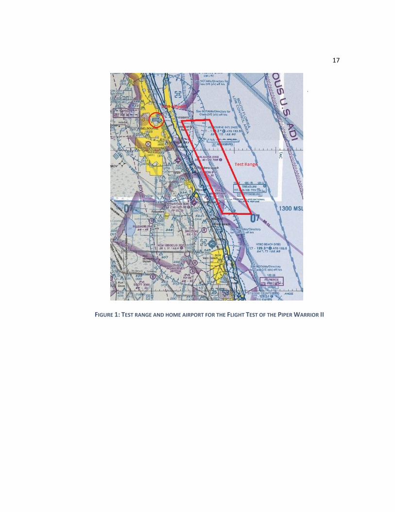
The first step for this flight test was the same as for any flight test, taxi, take-off,

and a flight to the test location. In this case the test flight was based out of Orlando-

Melbourne International Airport (KMLB). The test location was just off the eastern coast

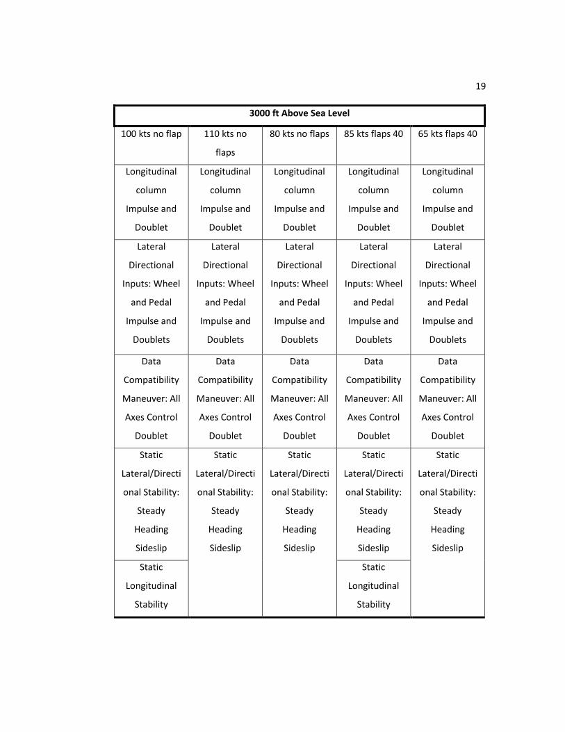
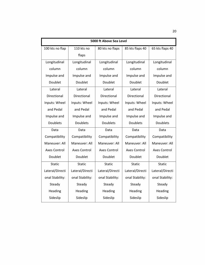
of Florida. The route the aircraft flew can be seen in Figure 1 below. Once at the test

location the following maneuvers were performed at varying altitudes, airspeeds, and flap

configurations. Table 2 below shows the full set of test configurations.

17

FIGURE 1: TEST RANGE AND HOME AIRPORT FOR THE FLIGHT TEST OF THE PIPER WARRIOR II

18

TABLE 2: TEST CONFIGURATIONS

1000 ft Above Sea Level

100 kts no flap 110 kts no

flaps

80 kts no flaps 85 kts flaps 40 65 kts flaps 40

Longitudinal

column Impulse

and Doublet

Longitudinal

column

Impulse and

Doublet

Longitudinal

column

Impulse and

Doublet

Longitudinal

column

Impulse and

Doublet

Longitudinal

column

Impulse and

Doublet

Lateral

Directional

Inputs: Wheel

and Pedal

Impulse and

Doublets

Lateral

Directional

Inputs: Wheel

and Pedal

Impulse and

Doublets

Lateral

Directional

Inputs: Wheel

and Pedal

Impulse and

Doublets

Lateral

Directional

Inputs: Wheel

and Pedal

Impulse and

Doublets

Lateral

Directional

Inputs: Wheel

and Pedal

Impulse and

Doublets

Data

Compatibility

Maneuver: All

Axes Control

Doublet

Data

Compatibility

Maneuver: All

Axes Control

Doublet

Data

Compatibility

Maneuver: All

Axes Control

Doublet

Data

Compatibility

Maneuver: All

Axes Control

Doublet

Data

Compatibility

Maneuver: All

Axes Control

Doublet

Static

Lateral/Directi

onal Stability:

Steady

Heading

Sideslip

Static

Lateral/Directi

onal Stability:

Steady

Heading

Sideslip

Static

Lateral/Directi

onal Stability:

Steady

Heading

Sideslip

Static

Lateral/Directi

onal Stability:

Steady

Heading

Sideslip

Static

Lateral/Directi

onal Stability:

Steady

Heading

Sideslip

19



flaps


Longitudinal

column

Impulse and

Doublet

Longitudinal

column

Impulse and

Doublet

Longitudinal

column

Impulse and

Doublet

Longitudinal

column

Impulse and

Doublet

Longitudinal

column

Impulse and

Doublet

Lateral

Directional

Inputs: Wheel

and Pedal

Impulse and

Doublets

Lateral

Directional

Inputs: Wheel

and Pedal

Impulse and

Doublets

Lateral

Directional

Inputs: Wheel

and Pedal

Impulse and

Doublets

Lateral

Directional

Inputs: Wheel

and Pedal

Impulse and

Doublets

Lateral

Directional

Inputs: Wheel

and Pedal

Impulse and

Doublets

Data

Compatibility

Maneuver: All

Axes Control

Doublet

Data

Compatibility

Maneuver: All

Axes Control

Doublet

Data

Compatibility

Maneuver: All

Axes Control

Doublet

Data

Compatibility

Maneuver: All

Axes Control

Doublet

Data

Compatibility

Maneuver: All

Axes Control

Doublet

Static

Lateral/Directi

onal Stability:

Steady

Heading

Sideslip

Static

Lateral/Directi

onal Stability:

Steady

Heading

Sideslip

Static

Lateral/Directi

onal Stability:

Steady

Heading

Sideslip

Static

Lateral/Directi

onal Stability:

Steady

Heading

Sideslip

Static

Lateral/Directi

onal Stability:

Steady

Heading

Sideslip

Static

Longitudinal

Stability

Static

Longitudinal

Stability

20



flaps


Longitudinal

column

Impulse and

Doublet

Longitudinal

column

Impulse and

Doublet

Longitudinal

column

Impulse and

Doublet

Longitudinal

column

Impulse and

Doublet

Longitudinal

column

Impulse and

Doublet

Lateral

Directional

Inputs: Wheel

and Pedal

Impulse and

Doublets

Lateral

Directional

Inputs: Wheel

and Pedal

Impulse and

Doublets

Lateral

Directional

Inputs: Wheel

and Pedal

Impulse and

Doublets

Lateral

Directional

Inputs: Wheel

and Pedal

Impulse and

Doublets

Lateral

Directional

Inputs: Wheel

and Pedal

Impulse and

Doublets

Data

Compatibility

Maneuver: All

Axes Control

Doublet

Data

Compatibility

Maneuver: All

Axes Control

Doublet

Data

Compatibility

Maneuver: All

Axes Control

Doublet

Data

Compatibility

Maneuver: All

Axes Control

Doublet

Data

Compatibility

Maneuver: All

Axes Control

Doublet

Static

Lateral/Directi

onal Stability:

Steady

Heading

Sideslip

Static

Lateral/Directi

onal Stability:

Steady

Heading

Sideslip

Static

Lateral/Directi

onal Stability:

Steady

Heading

Sideslip

Static

Lateral/Directi

onal Stability:

Steady

Heading

Sideslip

Static

Lateral/Directi

onal Stability:

Steady

Heading

Sideslip

21

2.4.1 Longitudinal column impulse and doublet

The purpose of the impulse was to establish a marker in the data file. The doublet

maneuver was used to get pitch data for both short and long period modes. This data was

then run through SIDPAC to find the dimensionless coefficients.

1. Trim Aircraft

2. Rapid column impulse at ½ input

3. Record for 10 seconds

4. Re-trim

5. Column doublet, targeting ±.5g


2.4.2 Lateral Directional Inputs: Wheel and Pedal Impulse and Doublets

The purpose of this maneuver was the same as the previous maneuver, but for rolling

and yawing data instead of pitch data, which is why a pedal doublet was necessary, since

the lateral and directional motions are coupled, data is needed for both aileron and

rudder inputs.

1. Trim Aircraft

2. Rapid wheel impulse at ½ input to the left


4. Rapid wheel impulse at ½ input to the right


6. Re-trim

7. Wheel doublet at ½ input


9. Pedal doublet at ½ input

10. Record for 3 Dutch-Roll cycles or until stable

22

11. Pedal doublet at full input

12. Record for 3 Dutch-Roll cycles or until stable

2.4.3 All Axes Control Doublet

Due to aircraft controls being coupled, an all axis control doublet helps relate the

effects of one input to the effects of another input. This should provide greater accuracy

for system identification, especially in a reversible control system like the one on the

Piper Warrior.

1. Trim Aircraft

2. Rapidly apply one after the other

a. Column doublet targeting ±.5g

b. Wheel doublet at ½ input

c. Pedal doublet at ½ input

3. Record Data for 3 Dutch Roll cycles or until stable

2.4.4 Static Longitudinal Stability

Data were gathered to determine static longitudinal stability. Positive static stability

means an airplane will tend to return to its trim condition following a disturbance. It also

is an indication of speed stability, where a pilot must push forward on the controls to

accelerate and pull back to decelerate from the trim condition.

1. Trim Aircraft

2. Decelerate 15 kts using aft column input. Do not change power or re-trim

3. Stabilize in 5 kt increments and record stick force

4. Relax and return to trim speed

5. Re-trim

6. Accelerate 15 kts using forward column input. Do not change power or re-trim

7. Stabilize in 5 kt increments and record stick force

8. Relax and return to trim speed

23

2.4.5 Static Lateral-Directional Stability, Steady Heading Sideslip

Data were gathered to determine static lateral-directional stability. Directional

stability (or weathercock stability) is the airplane’s tendency to return its trim sideslip

angle (which should be 𝛽 = 0) following a disturbance. Static lateral stability is the

tendency of the airplane to return to the trim bank angle following a disturbance. Unlike

longitudinal modes, lateral-directional modes are coupled.

1. Trim Aircraft

2. Nose Right SHSS

a. Do not adjust power

b. Descend as needed to maintain speed

c. Stabilize in 1/3 pedal increments

d. Hold for 5 seconds

3. Nose Left SHSS

a. Do not adjust power

b. Descend as needed to maintain speed

c. Stabilize in 1/3 pedal increments

d. Hold for 5 seconds

2.5 Data Reduction Procedure

After the test flight was performed and the data were gathered, the data had to be

analyzed. This was done using Dr. Eugene Morelli’s MATLAB SIDPAC program. To use this

complicated program, the data needs to be first loaded from excel. There are many was

to do this. It can be done manually or with automated commands as part of a larger

MATLAB script. Once all the data has been loaded in and assigned to the correct variables

in SIDPAC, the discontinuous data from the flight data should be smoothed using a

SIDPAC script ‘smoo.m’ which smooths out data taken at discrete time intervals and

makes it into more of a continuous input. This helps the accuracy of the parameter

24

estimates. The next step is to calculate the force and moment coefficients using

‘compfc.m’ and ‘compmc.m’ respectively, and then assign the values calculated to the

‘fdata’ array used by SIDPAC. Next the regressor matrix for equation-error parameter

estimation needs to be assembled which for a longitudinal maneuver uses the angle-of-

attack (alpha), the non-dimensional pitch rate (qhat), and the elevator input to solve.

Next smoothed trim values need to be found, and then removed from the regressors.

These are the smoothed values at the start of the time measurement. This is done to help

adjust for messy data at the beginning of the data collection window. If the data is already

really clean and smooth at the start, then this step doesn’t really do anything, but it is

relatively simple and always a good idea to perform. The next step is to prepare the

regressor matrix for use in ‘lesq.m’, which performs a least squares regression on the

matrix, which requires a constant regressor for the bias term. Then the z-force coefficient

stability and control derivatives are calculated using ‘lesq.m’. Once these are calculated

the parameter error bounds need to be calculated which is done using ‘r_colores.m’ and

then they can be displayed using ‘model_disp.m’. Next, stepwise regression needs to be

performed for the pitching moment coefficient. Part of this is to add a nonlinear cross

term, angle of attack*elevator angle, and then see what regressors should be added or

removed for the stepwise regression using ‘swr.m’. As part of this step the regressors get

added and removed by the user and a regressor should be kept only if it decreases fit

error, increases R2 value, and decreases the partial squared error. Then make sure that

the only parameters included are those for the selected regressors. Then, again calculate

and show the error bounds like before. Then the dimensional stability and control

derivatives need to be estimated using time-domain output-error estimation methods,

this is begun with ‘nldyn.m’ to set up the data for the output-error (oe) estimation. The

initial parameter values need to be found, but these come from the equation error

solution found before. Now, the estimation is begun using ‘oe.m’ and the model file

‘nldyn.m’ which is dynamic and so changes each time. This step takes a bit of time since it

has to run through several iterations to get as accurate a result as possible. Now the

25

estimated parameter error bounds are corrected using ‘m_colores.m’ and the results can

be viewed. The final piece of this estimation is to check the prediction capability by using

the data from another maneuver and the output-error model found before.

26

3 Chapter 3:

Results

The data gathered were run through SIDPAC to build aerodynamic models through

parameter estimation, which allows the force and moment coefficients to be calculated

for a variety of maneuvers and flight conditions in both the longitudinal axis and the

lateral axis. Positive inputs correspond to up elevator, right rudder, and right aileron.

Figure 2 shows the inputs and outputs from the test maneuver, in this case a control

column doublet at 5000 ft and 100 kts. As can be seen the elevator was trimmed at about

3.5 degrees up and was pulled to almost 6 degrees and then the push only needed to

drop a few degrees to apply the doublet according to the response motion. This data has

been smoothed out to allow for better calculations of the models and the moment

coefficients, but it has not been filtered in any way. The variables az and q are of

particular interest since they are used the most on the following plots. Az is the

acceleration in g’s in the z-direction, and q is the pitch rate in degrees per second.

27

FIGURE 2: FLIGHT TEST DATA FOR 5000 FT COLUMN DOUBLET

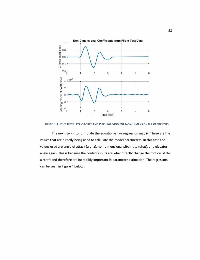
In Figure 3, the force and moment coefficients for longitudinal maneuvers such as

the column doublet can be seen. This is the data for the 5000ft column doublet. This data

comes from part of the standard aerodynamic equations and were solved along with the

Cl and Cd equations. Here you can see the effect of the smoothing done on the measured

flight test data in the previous steps. Force and moment coefficients are important since

they are a major part of the model formulation.

28

FIGURE 3: FLIGHT TEST DATA Z-FORCE AND PITCHING MOMENT NON-DIMENSIONAL COEFFICIENTS

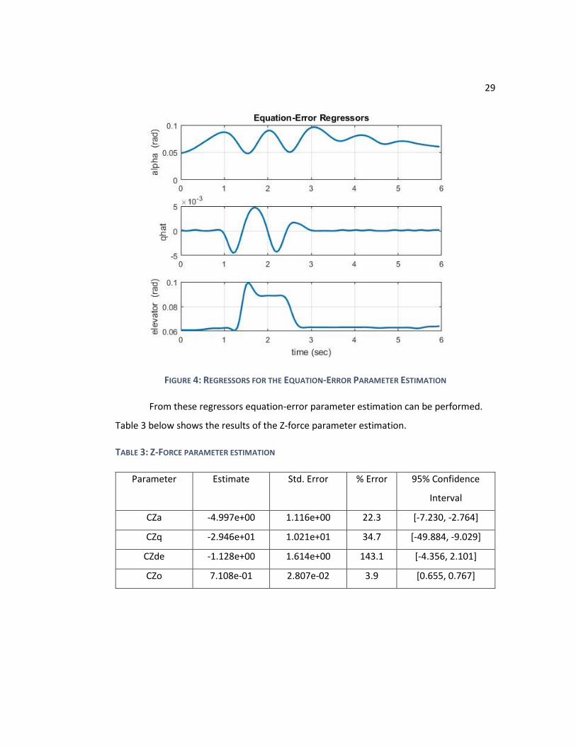
The next step is to formulate the equation-error regression matrix. These are the

values that are directly being used to calculate the model parameters. In this case the

values used are angle of attack (alpha), non-dimensional pitch rate (qhat), and elevator

angle again. This is because the control inputs are what directly change the motion of the

aircraft and therefore are incredibly important in parameter estimation. The regressors

can be seen in Figure 4 below.

29

FIGURE 4: REGRESSORS FOR THE EQUATION-ERROR PARAMETER ESTIMATION

From these regressors equation-error parameter estimation can be performed.

Table 3 below shows the results of the Z-force parameter estimation.

TABLE 3: Z-FORCE PARAMETER ESTIMATION

Parameter Estimate Std. Error % Error 95% Confidence

Interval

CZa -4.997e+00 1.116e+00 22.3 [-7.230, -2.764]

CZq -2.946e+01 1.021e+01 34.7 [-49.884, -9.029]

CZde -1.128e+00 1.614e+00 143.1 [-4.356, 2.101]

CZo 7.108e-01 2.807e-02 3.9 [0.655, 0.767]

30

As can be seen, the percent error for each parameter is decently low for all but

CZde, which is the Coefficient of Z-force from the change in elevator angle, but even then,

the 95% confidence interval is pretty small. Figure 5 shows the plot of the prediction from

the regression model compared to the flight data as well as the residual between the two.

It can be seen that although the percent error in the parameters was decently large the

model compared to the flight data wasn’t drastically inaccurate.

FIGURE 5: EQUATION-ERROR PARAMETER ESTIMATION RESULTS

Now the next step is to perform the estimation for the pitching moment

coefficient which is performed though the use of step-wise regression. This allows for the

addition and removal of regressors to ensure that they do not harm the overall model fit.

Each parameter can be seen below, but in the overall model fit the first parameter has

been left out because it did not change the R2 value very much and showed other signs of

31

damaging the overall model, the direct plot of the model being one of these. Table 4

shows the estimates and change from the addition of each parameter for the pitching

moment coefficient. In the end result though the model was the best when parameter 1

was removed.

TABLE 4: STEP-WISE REGRESSION FOR THE PITCHING MOMENT COEFFICIENT

Parameter Estimate Fit Error R2 Partial Squared

Error

1 -6.9740e+03 83.03% 32.21% 1.5519e+04

2 -1.5862e+04 81.70% 44.93% 1.5101e+04

3 9.7539e+02 81.76% 35.38% 1.5187e+04

4 -5.8894e+05 56.70% 69.19% 7.8211e+03

So, then the projected model can be seen in Figure 6 below. It can be seen that

the model matches the flight data pretty well even if it is not exact, this plot fits better

than it did with parameter 1 included. The residual between the flight data and equation-

error model can be seen as well and other than a couple points is also not too major.

32

FIGURE 6: PITCHING MOMENT COEFFICIENT MODEL PLOTTED OVER FLIGHT DATA

Table 5 below shows the value of the estimates as well as the associated percent error,

standard error and 95% confidence interval. This shows that each of the parameters are

very large for this model, even though the z-force models were much smaller.

TABLE 5: PITCHING MOMENT ESTIMATED PARAMETERS

Parameter Estimate Std. Error %

Error

95% Confidence

Interval

Cma -3.395e+04 9.689e+03 28.5 [-53326.423, -

14570.162]

Cmq 1.367e+04 1.915e+03 14.0 [9841.450, 17502.690]

Cmde -6.644e+05 7.394e+04 11.1 [-812239.891, -

516484.018]

Cmo -1.237e+01 1.1112e+01 89.9 [-34.611, 9.875]

33

So now output-error in the time domain is needed. This uses the previous steps as

a starting point and solves for overall parameter estimation. It essentially refines the

models to better fit the flight data. This model fits a set of new flight data, it is mostly the

same as before but q, the pitch rate in radians per second, is also included. This can be

seen in Figure 7 below.

FIGURE 7: OUPUT-ERROR TIME DOMAIN MODELING FLIGHT DATA

The output-error method is an iterative method that runs through many revisions trying

to get convergence on the model. For this data it ran for approximately 72 seconds. The

end model can be seen and compared to the flight data below in Figure 8.

34

FIGURE 8: OUTPUT-ERROR PARAMETER ESTIMATION MODEL VS. FLIGHT DATA

The accuracy of the model can be seen here. In general, the model is decent, but

the pitch rate shows almost no prediction at all in the model. This may be caused by many

different things. The most likely is that none of the data was corrected for the location of

the sensors. This causes issues since all the forces and moments act through the Center of

Gravity (CG) of the aircraft so if the sensor locations are not over the CG then the data

ends up being inaccurate. Another source of error is that which also causes the errors

seen in previous steps, which is that much of the flight data has no filter on it. This causes

an enormous amount of scatter in the data readings and in fact can be seen in the angle-

of-attack (alpha) in Figure 8 above. The flight data shows that both the pitch rate and the

z-axis acceleration levels off to a constant after the maneuver ends at approximately the 3

second mark. The angle-of-attack though does not. This should not happen, if anything

the angle of attack should level out before or at the same time as the others. Especially

since the angle of attack is a measure of the relative wind axis. If the aircraft is not

changing pitch, then alpha should not be changing either unless the aircraft is hit by gusts

or turbulence. But in the plot above the change in alpha is too consistent to be caused by

35

random irregular events like gusts and turbulence. This leads to the conclusion that the

lack of filtering and use of smoothing causes the oscillation in alpha and leads to a

degraded model, building the model without smoothing the data led to a much worse

estimation.

TABLE 6: PARAMETER ESTIMATION RESULTS

Parameter Estimate Std. Error %Error 95% Confidence Interval

CZa -4.520e+00 2.083e+00 46.1 [-8.685, -0.355]

CZq 3.578e+01 1.847e+01 51.6 [-1.163, 72.725]

CZde -3.522e+00 9.119e-01 25.9 [-5.346, -1.698]

CZo -4.495e-01 5.545e-02 12.3 [-0.560, -.0339]

Cma -3.859e+04 1.342e+04 34.8 [-65423.706, -11752.094]

Cmq 1.987e+04 4.839e+05 2434.8 [-947905.765, 987653.328]

Cmde 1.642e+04 1.077e+04 65.6 [-5115.984, 37958.824]

Cmo 6.836e+02 3.876e+02 56.7 [-91.496, 1458.735]

azo 1.973e+00 2.946e-02 1.5 [1.915, 2.032]

The results of the poor model estimate for the pitch rate q can be seen very

obviously in the % Error for the parameter Cmq, in this case it is 2434.8% seen in Table 6

above. This is an insanely high error, and means that it is still completely unknown, which

makes sense with the plot of the model in Figure 8 that was looked at earlier. Again,

filtered data would probably help clean these models up and hopefully give a true model

for the longitudinal movement of the Piper Warrior II.

Once the longitudinal model has been found, the lateral model needs to be

computed. This is performed using the same steps as in the longitudinal model, but the

effects of multiple control inputs, both aileron and rudder, as well as both rolling and

yawing moment. In Figure 9 below the control inputs and outputs can be seen. Lateral

36

movements of the aircraft are influenced by both rudder inputs and aileron inputs and

measured in yaw angle, roll angle, and sideslip angle.

FIGURE 9: LATERAL FLIGHT TEST DATA

Like before, all this data has been smoothed to build better models. Here it can

be seen that the primary control input was a rudder doublet. While the aileron also

moved, it is less defined as the maximum and minimum are not the same, nor are they

applied for the same amount of time. Instead these are likely just the result of the

aircrafts motion during the doublet. In fact, the rudder input clearly shows a maximum for

about half a second then a minimum for the same length of time. This would correspond

to a full input in one direction, then a full input in the other.

37

FIGURE 10: Y-FORCE AND ROLLING MOMENT COEFFICIENTS FOR LATERAL MANEUVER

The non-dimensional coefficients in Figure 10 above are the key to the lateral

models. It can be seen that the Y-force coefficient has a decently smooth curve, but the

rolling moment has much sharper peaks and valleys. Now that the Y-force and rolling

moment coefficients have been calculated the regressor matrix for least squares

regression needed to be built. These regressors are shown in Figure 11 seen below.

38

FIGURE 11: EQUATION ERROR REGRESSORS FOR LATERAL MODEL

Using the regressors seen in Figure 11 the Y-Force parameter estimates are

calculated using a least-squares equation-error regression. The results can be seen below

in

Table 7. Note the high percent error on the Y-Force coefficient from the side slip

angle Beta (CYb). The model result can be seen in Figure 12 below; the model matches

the flight data pretty well, which means that the high percent error in

Table 7 for CYb just means that its effect on the model may be drastically

different than that shown. On the other hand, though, since both the estimate and the

standard error are so small, CYb probably doesn’t affect the model very much.

39

TABLE 7: Y-FORCE PARAMETER ESTIMATION

Parameter Estimate Std. Error % Error 95% Confidence

Interval

CYb 7.267e-02 1.247e-01 171.7 [-0.177, 0.322]

CYp 4.059e+00 7.171e-01 17.7 [2.625, 5.494]

CYdr -7.242e-02 3.066e-02 42.3 [-0.134, -0.011]

CYda -2.019e-01 8.468e-02 41.9 [-0.371, -0.033]

CYo 8.163e-03 2.217e-03 27.2 [0.004, 0.013]

FIGURE 12:Y-FORCE EQUATION-ERROR PARAMETER ESTIMATION MODEL

So according to the comparison plot the Y-Force model is very accurate with low

residuals across most of it. This means that the next step is to move onto the rolling and

yawing moment models. First the rolling moment coefficient parameters are determined

40

through step-wise regression. The results of which can be seen in Table 8 below and the

model plot can be seen in Figure 13 below.

TABLE 8: STEP-WISE REGRESSION FOR ROLLING MOMENT LATERAL MANEUVER


Error

1 5.6994e+02 88.88% 21.62% 3.5998e+03

2 2.8557e+03 76.54% 42.11% 2.6864e+03

3 -3.1145e+02 56.85% 68.19% 1.5191e+03

4 -1.6575e+02 56.71% 68.48% 1.5239e+03

5 -3.1493e+02 53.42% 72.15% 1.3756e+03

When the model was built, the 4th parameter was left out of the model. This is

because during the step-wise regression the 4th parameter showed very minor

improvements on the overall model and showed that it was a superfluous parameter that

just complicated and obfuscated the model.

41

FIGURE 13: ROLLING MOMENT MODEL USING STEP-WISE REGRESSION

Since the 4th parameter was removed from the step-wise regression the

parameters of the rolling moment model can be seen in Table 9 below. It should be noted

that although the percent error for each parameter is much less overall than previously,

the model is less accurate to the flight data. This means that the effect the parameters

have on the model are much more accurately predicted than for the Y-force coefficient

model.

TABLE 9: ROLLING MOMENT PARAMETER ESTIMATION RESULTS

Parameter Estimate Std. Error %Error 95% Confidence

Interval

Crb 5.699e+02 8.481e+01 14.9 [400.330, 739.554]

Crp 2.856e+03 9.979e+02 34.9 [859.962, 4851.385]

Crdr -3.115e+02 8.339e+01 26.8 [-478.236, -144.664]

Crda -2.839e+02 1.866e+02 65.7 [-657.073, 89.368]

42

Cro 1.160e+01 5.011 e+00 43.2 [1.581, 21.627]

Now that the rolling moment model has been found the Yawing moment can also

be calculated. This model is solved much the same way as the rolling moment model, but

only taking into consideration yaw, rather than roll. This model uses the same inputs as

the rolling moment model and as before the 4th parameter was left out of the final model

due to the low improvements and the fact that it had a high correlation with the third

parameter and therefore should have been left out of the model formulation.

TABLE 10: STEP-WISE REGRESSION FOR YAWING MOMENT LATERAL MANEUVER


Error

1 7.3389e+00 90.28% 19.03% 2.2964e+02

2 -4.1035e+02 86.74% 25.55% 2.1245e+02

3 1.8425e+01 85.27% 28.34% 2.0573e+02

4 -3.3868e+01 85.19% 28.77% 2.0566e+02

Table 10 and Table 11, above and below, show the step-wise regression and parameter

estimates. This model shows incredibly high percent errors on the parameters and the

low R2 value during the step-wise regression leads to one explanation of that. Since the R2

value is the easiest indication of how well the parameters are going to fit the model, how

low it was throughout the step-wise regression showed that the parameter estimation

was unlikely to be accurate.

43

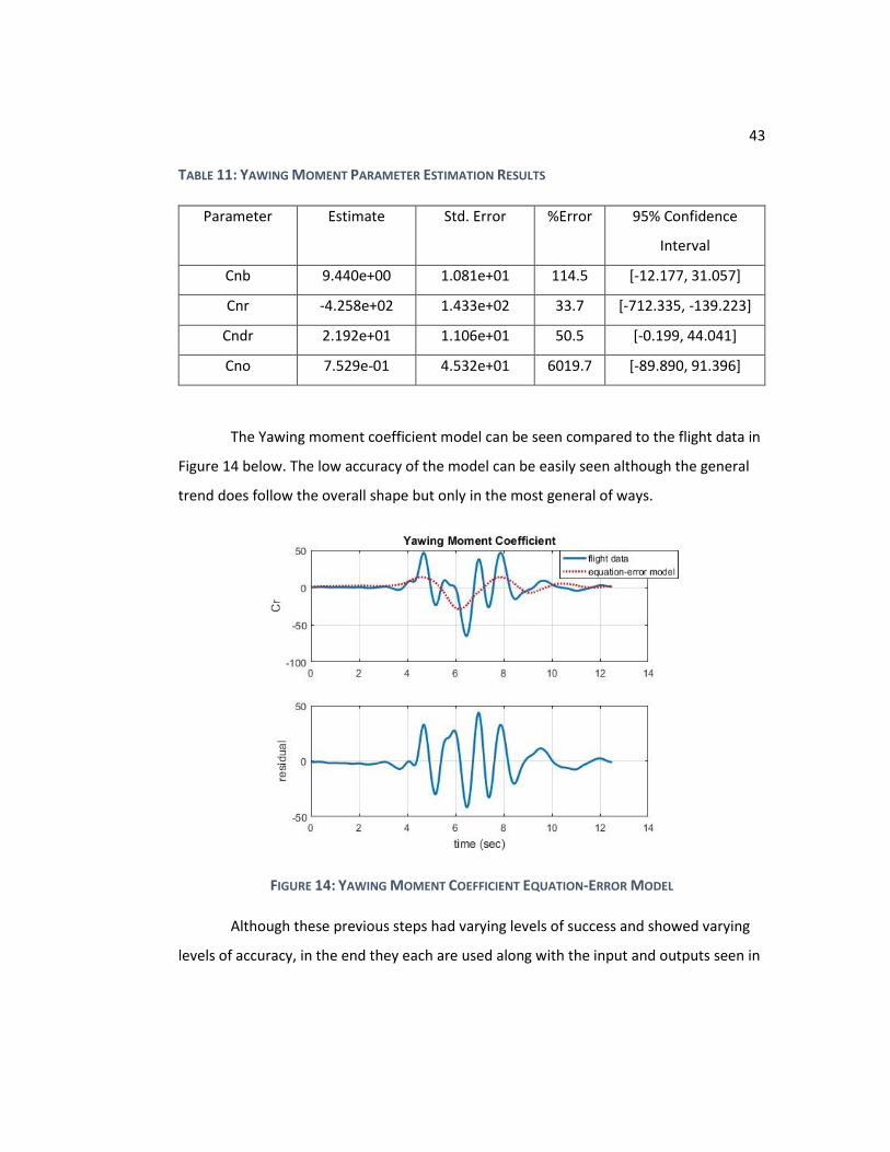
TABLE 11: YAWING MOMENT PARAMETER ESTIMATION RESULTS


Interval

Cnb 9.440e+00 1.081e+01 114.5 [-12.177, 31.057]

Cnr -4.258e+02 1.433e+02 33.7 [-712.335, -139.223]

Cndr 2.192e+01 1.106e+01 50.5 [-0.199, 44.041]

Cno 7.529e-01 4.532e+01 6019.7 [-89.890, 91.396]

The Yawing moment coefficient model can be seen compared to the flight data in

Figure 14 below. The low accuracy of the model can be easily seen although the general

trend does follow the overall shape but only in the most general of ways.

FIGURE 14: YAWING MOMENT COEFFICIENT EQUATION-ERROR MODEL

Although these previous steps had varying levels of success and showed varying

levels of accuracy, in the end they each are used along with the input and outputs seen in

44

Figure 15 below. While much of this is the same as previous steps, it is important to note

the plot of the yaw rate (r). The yaw rate shows as a horizontal line at zero. This is

because during the test flights of the aircraft the heading at the start of the maneuver

was not recorded and because the only heading data came from a GPS reading any cross

wind would change the heading that was recorded. So while a magnetic compass will

show you where the aircraft is pointing but not necessarily where it is going and a GPS

can do both, what was recorded was the direction the aircraft was flying not necessarily

where it was pointing. This combined with the lack of a start heading for the maneuver

made calculation of the yaw rate impossible for this test.

FIGURE 15: OUTPUT-ERROR MODELLING FLIGHT DATA

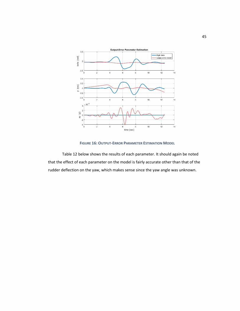
Nonetheless, a model was built leaving this data out and can be seen in Figure 16 below.

Here the model very clearly does not match up to the flight data but again it shows a

general trend toward what the flight data showed the aircraft doing.

45

FIGURE 16: OUTPUT-ERROR PARAMETER ESTIMATION MODEL

Table 12 below shows the results of each parameter. It should again be noted

that the effect of each parameter on the model is fairly accurate other than that of the

rudder deflection on the yaw, which makes sense since the yaw angle was unknown.

46

TABLE 12: LATERAL PARAMETER ESTIMATION RESULTS


Interval

CYb 7.648e-01 4.628e-01 60.5 [-0.161, 1.691]

CYp -3.010e-01 8.029e-02 26.7 [-0.462, -0.140]

CYdr 5.378e-02 3.604e-02 67.0 [-0.018, 0.126]

CYda 6.5969e+02 2.595e+02 39.5 [137.931, 1175.783]

CYo -4.349e+02 1.700e+02 39.1 [-774.917, -94.808]

Crb 5.633e+02 1.373e-09 0.0 [563.322, 563.322]

Crp 4.184e+01 1.071e+01 25.6 [20.426, 63.248]

Crdr -1.414e+02 3.508e+01 24.8 [-211.586, -71.260]

Crda 5.009e+01 1.719e+01 34.3 [15.719, 84.464]

Cro -6.902e+01 2.478e+01 35.9 [-118.573, -19.465]

Cnb 7.025e+01 2.961e+01 42.1 [11.041, 129.466]

Cnp -4.351e+02 1.544e-12 0.0 [-435.053, -435.053]

Cndr -1.505e+00 1.976e+00 131.3 [-5.457, 2.448]

Cnbr 2.017e+01 4.798e+00 23.8 [10.574, 29.764]

Cno -6.467e+00 1.757e+00 27.2 [-9.981, -2.954]

ayo 6.964e-02 8.425e-03 12.1 [0.053, 0.086]

In summary, longitudinal and lateral-directional models were built from flight test

data. Not correcting for the sensor location, the lack of a good filter on much of the data,

and the difficulty in finding yaw angles all impacted the quality of the models. Therefore,

the derived models are not yet suitable for use in either simulation or design. That being

said, applying a good filter to the flight test data and correcting for the sensor locations

should result in better models.

47

4 Conclusion

4.1 Conclusion

The purpose of testing the Piper Warrior II was to build an aerodynamic model for

the flight characteristics of the aircraft. This was accomplished through several different

maneuvers designed to produce a measurable output from a known control input so that

the responses could be modeled mathematically. Longitudinal data were recorded using

column doublets, while lateral data came from pedal doublets. Doublets were used to

keep a good frequency range so that more accurate models could be built. The models

showed that further work is needed building upon what was done here. This is for several

reasons, the first is because the lack of filters led to very messy data and poor models.

Another reason is because the heading at the start of each maneuver was not recorded

and therefore the yaw angle and yaw rate could not be calculated. The final and most

important source of error was that the Garmin G5 data was not corrected for the location

of the sensor in the aircraft.

4.2 Future Work

In the future, more work should be done to build better models and gather more

accurate parameters for the Warrior II. A filter of some sort should be placed over the

data that does not show smooth lines. For example, the AoA and AoS data were both very

messy data sets and should have an appropriate filter run over them to better model the

effects the controls had on them and the effects they had on the controls. Another thing

that could be done would be to run the calculations in the frequency domain instead of

the time domain. This may also help to clean up the models a great deal, since real world

interference is accounted for much better in the frequency domain. The final thing that

could improve the models is to correct for the location of the sensors. Since neither data

48

source was located at the cg variations in the measurements were introduced and should

be accounted for. There are several ways to do so but the easiest would be to re-fly the

tests with the Garmin G5 located over the cg. This would mean that location corrections

would not be needed. On the other hand, this would cost more since the tests would

need to be flown again and another Garmin probably acquired, though this would also

allow for the recording of the heading at the start of each maneuver and the yaw angle

then measured.

49

5 References

[1] Dunbar, B., “Wind Tunnels,” NASA Available:

https://www.nasa.gov/centers/ames/research/lifeonearth/lifeonearth-

windtunnels.html.

[2] Grauer, J. A., and Morelli, E. A., “Generic Global Aerodynamic Model for Aircraft,”

Journal of Aircraft, vol. 52, Jul. 2014, pp. 13–20.

[3] Jategaonkar, R. V., Fischenberg, D., and Gruenhagen, W., “Aerodynamic Modeling

and System Identification from Flight Data-Recent Applications at DLR,” Journal of

Aircraft, vol. 41, 2004, pp. 681–691.

[4] Klein, V., Morelli, E. Aircraft System Identification Theory and Practice, edited by J.

A. Schultz AIAA Education Series, AIAA, Virginia, 2006

[5] Liu, J., Li, S., Song, X., and Wang, C., “Influence of linear and nonlinear

aerodynamic models on parameter identification for aircraft,” 2017 International

Conference on Control, Automation and Information Sciences (ICCAIS), Dec. 2017.

[6] Murphy, P. C., Klein, V., and Frink, N. T., “Nonlinear Unsteady Aerodynamic

Modeling Using Wind Tunnel and Computational Data - Invited,” AIAA

Atmospheric Flight Mechanics Conference, Nov. 2016.

[7] “The NACA/NASA Full Scale Wind Tunnel,” National Air and Space Museum

Available: https://airandspace.si.edu/stories/editorial/nacanasa-full-scale-wind-

tunnel.

[8] Piper Aircraft Corporation, “Warrior II PA-28-151 Pilot’s Operating Handbook,”

Section 1 General, Vero Beach, Florida, 1982, pp. 1-4

[9] Piper Aircraft Corporation, “Warrior II PA-28-151 Pilot’s Operating Handbook,”

Section 6 Weight and Balance, Vero Beach, Florida, 1982, pp. 6-14

[10] Rose, I. D., “Aerodynamic modeling of an unmanned aerial vehicle using a

computational fluid dynamics prediction code,” thesis, 2009.

https://www.nasa.gov/centers/ames/research/lifeonearth/lifeonearth-windtunnels.html

https://www.nasa.gov/centers/ames/research/lifeonearth/lifeonearth-windtunnels.html

https://airandspace.si.edu/stories/editorial/nacanasa-full-scale-wind-tunnel

https://airandspace.si.edu/stories/editorial/nacanasa-full-scale-wind-tunnel

50

6 Appendices 6.1 Appendix A: SIDPAC MatLab Codes 6.1.1 deriv.m

function zd = deriv(z,dt) % % DERIV Smoothed numerical differentiation. % % Usage: zd = deriv(z,dt); % % Description: % % Computes smoothed derivatives of measured time series % by differentiating a local quadratic least-squares fit % to the set of points consisting of each data point % and its four nearest neighboring points. % % Input: % % z = vector or matrix of measured time series. % dt = sampling interval, sec. % % Output: % % zd = vector or matrix of smoothed time derivatives. %

% % Calls: % None % % Author: Eugene A. Morelli % % History: % 13 Jan 1996 - Created and debugged, EAM. % 06 Sept 2001 - Modified to accept row or column

vectors, EAM. % % Copyright (C) 2006 Eugene A. Morelli % % This program carries no warranty, not even the implied % warranty of merchantability or fitness for a particular

purpose. % % Please email bug reports or suggestions for improvements

to: %

51

% [email protected] % [m,n]=size(z); zd=zeros(m,n); % % Put data in column vectors if necessary, % and set the number of data points. % if m < n zd=zd'; z=z'; npts=n; else npts=m; end % % Analytic expressions for the derivative of local % polynomial fits to the noisy measured data. % The expressions are different near the endpoints % because there are not enough neighboring points on one

side. % zd(1,:)=(-54*z(1,:)+13*z(2,:)+40*z(3,:)+27*z(4,:)... -26*z(5,:))/(70*dt); zd(2,:)=(-34*z(1,:)+3*z(2,:)+20*z(3,:)+17*z(4,:)... -6*z(5,:))/(70*dt); zd(3:npts-2,:)=(-2.*z(1:npts-4,:)-z(2:npts-3,:)+z(4:npts-

1,:)... +2.*z(5:npts,:))/(10.*dt); zd(npts-1,:)=(34*z(npts,:)-3*z(npts-1,:)-20*z(npts-2,:)... -17*z(npts-3,:)+6*z(npts-4,:))/(70*dt); zd(npts,:)=(54*z(npts,:)-13*z(npts-1,:)-40*z(npts-2,:)... -27*z(npts-3,:)+26*z(npts-4,:))/(70*dt); % % Switch data back to original form, if necessary. % if m < n zd=zd'; z=z'; end return

6.1.2 smoo.m

function [zs,fco,rr,b,f,wf,gv,sigab,nseab] =

smoo(z,t,fcep,lplot,auto) %

52

% SMOO Optimal global Fourier smoothing. % % Usage: [zs,fco,rr,b,f,wf,gv,sigab,nseab] =

smoo(z,t,fcep,lplot,auto); % % Description: % % Computes smoothed time series and noise covariance

matrix % estimates from measured data, using optimal Fourier

smoothing. % The analyst can select signal cut-off frequency % for the deterministic signal, based on the Lanczos sine

series % spectrum. Inputs fcep, lplot, and auto are optional. % % Input: % % z = vector or matrix of measured time series. % t = time vector. % fcep = cutoff frequency for low pass filtering % of the endpoints, Hz (default = 1). % lplot = plot flag: % = 1 for smoothing plots. % = 0 to skip the plots (default). % auto = flag indicating type of operation: % = 1 for automatic (no user input required,

default). % = 0 for manual (user input required). % % Output: % % zs = vector or matrix of smoothed time series. % fco = scalar or vector of cutoff frequencies, Hz. % rr = scalar or matrix discrete noise covariance

estimate. % b = vector or matrix of Fourier sine series

coefficients % for detrended time series reflected about the

origin. % f = vector of frequencies for the Fourier % sine series coefficients, Hz. % wf = vector or matrix of filter weights in the

frequency domain. % gv = vector or matrix of measured time series % with endpoint discontinuities removed. % sigab = vector or matrix frequency-domain model of % the absolute Fourier sine coefficients

53

% for the deterministic part of the measured time

series. % nseab = scalar or vector of the constant frequency-domain % model of the absolute Fourier sine coefficients % for the random noise part of the measured time

series. %

% % Calls: % xsmep.m % fsinser.m % mfilt.m % wnfilt.m % compzs.m % rrest.m % freqcut.m % % Author: Eugene A. Morelli % % History: % 14 Mar 1993 - Created and debugged, EAM. % 01 Aug 1999 - Modified for manual operation, EAM. % 18 Jan 2000 - Modified plotting for SID use, EAM. % 15 Sept 2000 - Modified to include option for % automatic Wiener filtering, EAM. % % Copyright (C) 2006 Eugene A. Morelli % % This program carries no warranty, not even the implied % warranty of merchantability or fitness for a particular


to: % % [email protected] % [npts,n]=size(z); dt=1/round(1/(t(2)-t(1))); % % Provide default inputs, if necessary. % if nargin < 5, auto=1; end if nargin < 4, lplot=0; end

54

if nargin < 3, fcep=1.0; end if lplot==1 Fg2H=figure('Units','normalized',... 'Position',[0.492 0.360 0.504 0.556],... 'Color',[0.8 0.8 0.8],... 'Name','Smoother Plots',... 'NumberTitle','off',... 'ToolBar','none'); end % % Smooth the endpoints. % zsmep=xsmep(z,fcep,dt); % % Reflect the time history about the time origin, % and expand in a Fourier sine series. % [b,f,gv]=fsinser(zsmep,dt); % % Manual ideal filtering or automatic Wiener filtering. % if auto==0 wf=mfilt(b,f); % % Signal and noise models for the ideal filter. % sigab=abs(b).*wf; nseab=ones(size(b)); % % Find cut-off frequencies from the filter. % fco=freqcut(wf,dt); % % Implement the Wiener filter for the manual case. % Compute signal and noise models for the Wiener % filter by normalizing the signal and noise models % so they both equal one at the cut-off frequency. % for j=1:n, sigab(:,j)=ones(npts,1)./((f/fco(j)).^3); nseab(:,j)=ones(npts,1); wf(:,j)=(sigab(:,j).^2)./(sigab(:,j).^2+nseab(:,j).^2); end else [wf,sigab,nseab]=wnfilt(b); % % Find cut-off frequencies from the filters.

55

% fco=freqcut(wf,dt); end % % Construct the smoothed signals. % zs=compzs(zsmep,wf,b); % % Estimate the noise variances. % rr=rrest(z,zs); if lplot==1, for j=1:n, fprintf(1,'\n\n Plots for Signal # %i\n',j), clf; subplot(3,1,1),plot(t,z(:,j)),ylabel('z'),grid on, subplot(3,1,2),plot(t,zs(:,j)),ylabel('zs'),grid on, subplot(3,1,3),plot(t,z(:,j)-zs(:,j)),ylabel('z-zs'), xlabel('time (sec)'),grid on, fprintf('\n\n Frequency cut-off at %4.1f Hz ',fco(j)); if n > 1 fprintf('for signal # %i\n\n',j); else fprintf('\n\n') end if j < n fprintf('\n Press any key to continue ... '),pause, end end fprintf('\n Press any key to continue ... '),pause, fprintf('\n\n'), close(Fg2H), else for j=1:n, fprintf('\n\n Frequency cut-off at %4.1f Hz ',fco(j)); if n > 1 fprintf('for signal # %i\n\n',j); else fprintf('\n\n'), end end end return

6.1.3 compfc.m and compmc.m

6.1.3.1 compfc.m

56

function [CX,CY,CZ,CD,CYw,CL,CT,phat,qhat,rhat] =

compfc(fdata,cbar,bspan,sarea) % %[fdata(:,61),fdata(:,62),fdata(:,63),fdata(:,67),fdata(:,68

),fdata(:,69),fdata(:,70),fdata(:,71),fdata(:,72),fdata(:,73

)]=compfc(fdata) % % COMPFC Computes non-dimensional force coefficients. % % Usage: [CX,CY,CZ,CD,CYw,CL,CT,phat,qhat,rhat] =

compfc(fdata,cbar,bspan,sarea); % % Description: % % Computes the non-dimensional force coefficients % and non-dimensional angular rates based % on measured flight data from input data array fdata. % Inputs cbar, bspan, and sarea can be omitted if % fdata contains this information. % % Input: % % fdata = flight data array in standard configuration. % cbar = wing mean aerodynamic chord, ft. % bspan = wing span, ft. % sarea = wing area, ft2. % % Output: % % CX = non-dimensional body-axis X coefficient. % CY = non-dimensional body-axis Y coefficient. % CZ = non-dimensional body-axis Z coefficient. % CD = non-dimensional stability-axis drag coefficient. % CYw = non-dimensional wind-axis side force

coefficient. % CL = non-dimensional stability-axis lift coefficient. % CT = non-dimensional thrust coefficient. % phat = non-dimensional roll rate. % qhat = non-dimensional pitch rate. % rhat = non-dimensional yaw rate. %

% % Calls: % None % % Author: Eugene A. Morelli % % History:

57

% 13 Jan 2000 - Created and debugged, EAM. % 07 Sept 2001 - Modified to include time-varying mass,

EAM. % 12 July 2002 - Made geometry inputs optional, EAM. % 15 Sept 2004 - Added error checks for airspeed and

qbar, EAM. % 30 May 2006 - Corrected CD and CL descriptive

comments, EAM. % % Copyright (C) 2006 Eugene A. Morelli % % This program carries no warranty, not even the implied % warranty of merchantability or fitness for a particular


to: % % [email protected] % [npts,n]=size(fdata); dtr=pi/180; g=32.174; if nargin < 4 sarea=fdata(1,77); end if nargin < 3 bspan=fdata(1,78); end if nargin < 2 cbar=fdata(1,79); end if ((sarea <=0) || (bspan <= 0) || (cbar <= 0)) fprintf('\n\n Geometry input error in compfc.m \n\n') return end if (norm(fdata(:,2))==0) fprintf('\n\n Zero airspeed error in compfc.m \n\n') return end if (norm(fdata(:,27))==0) fprintf('\n\n Zero qbar error in compfc.m \n\n') return end qbars=sarea*fdata(:,27); mass=fdata(:,48); CT=sum(fdata(:,[38:41])')'./qbars; CX=g*mass.*fdata(:,11)./qbars - CT; CY=g*mass.*fdata(:,12)./qbars;

58

CZ=g*mass.*fdata(:,13)./qbars; alfa=fdata(:,4)*dtr; beta=fdata(:,3)*dtr; CD=-CX.*cos(alfa) - CZ.*sin(alfa); CL=CX.*sin(alfa) - CZ.*cos(alfa); % CDw=CD.*cos(beta) - CY.*sin(beta); CYw=CY.*cos(beta) + CD.*sin(beta); phat=fdata(:,5)*dtr*bspan./(2*fdata(:,2)); qhat=fdata(:,6)*dtr*cbar./(2*fdata(:,2)); rhat=fdata(:,7)*dtr*bspan./(2*fdata(:,2)); % phat=fdata(:,5)*dtr*bspan./(2*mean(fdata(:,2))); % qhat=fdata(:,6)*dtr*cbar./(2*mean(fdata(:,2))); % rhat=fdata(:,7)*dtr*bspan./(2*mean(fdata(:,2))); return

6.1.3.2 compmc.m function [CX,CY,CZ,CD,CYw,CL,CT,phat,qhat,rhat] =

compfc(fdata,cbar,bspan,sarea) % %[fdata(:,61),fdata(:,62),fdata(:,63),fdata(:,67),fdata(:,68)

,fdata(:,69),fdata(:,70),fdata(:,71),fdata(:,72),fdata(:,73)]

=compfc(fdata) % % COMPFC Computes non-dimensional force coefficients. % % Usage: [CX,CY,CZ,CD,CYw,CL,CT,phat,qhat,rhat] =

compfc(fdata,cbar,bspan,sarea); % % Description: % % Computes the non-dimensional force coefficients % and non-dimensional angular rates based % on measured flight data from input data array fdata. % Inputs cbar, bspan, and sarea can be omitted if % fdata contains this information. % % Input: % % fdata = flight data array in standard configuration. % cbar = wing mean aerodynamic chord, ft. % bspan = wing span, ft. % sarea = wing area, ft2. % % Output: % % CX = non-dimensional body-axis X coefficient. % CY = non-dimensional body-axis Y coefficient. % CZ = non-dimensional body-axis Z coefficient.

59

% CD = non-dimensional stability-axis drag coefficient. % CYw = non-dimensional wind-axis side force coefficient. % CL = non-dimensional stability-axis lift coefficient. % CT = non-dimensional thrust coefficient. % phat = non-dimensional roll rate. % qhat = non-dimensional pitch rate. % rhat = non-dimensional yaw rate. %

% % Calls: % None % % Author: Eugene A. Morelli % % History: % 13 Jan 2000 - Created and debugged, EAM. % 07 Sept 2001 - Modified to include time-varying mass,

EAM. % 12 July 2002 - Made geometry inputs optional, EAM. % 15 Sept 2004 - Added error checks for airspeed and

qbar, EAM. % 30 May 2006 - Corrected CD and CL descriptive

comments, EAM. % % Copyright (C) 2006 Eugene A. Morelli % % This program carries no warranty, not even the implied % warranty of merchantability or fitness for a particular


to: % % [email protected] % [npts,n]=size(fdata); dtr=pi/180; g=32.174; if nargin < 4 sarea=fdata(1,77); end if nargin < 3 bspan=fdata(1,78); end if nargin < 2 cbar=fdata(1,79); end if ((sarea <=0) || (bspan <= 0) || (cbar <= 0))

60

fprintf('\n\n Geometry input error in compfc.m \n\n') return end if (norm(fdata(:,2))==0) fprintf('\n\n Zero airspeed error in compfc.m \n\n') return end if (norm(fdata(:,27))==0) fprintf('\n\n Zero qbar error in compfc.m \n\n') return end qbars=sarea*fdata(:,27); mass=fdata(:,48); CT=sum(fdata(:,[38:41])')'./qbars; CX=g*mass.*fdata(:,11)./qbars - CT; CY=g*mass.*fdata(:,12)./qbars; CZ=g*mass.*fdata(:,13)./qbars; alfa=fdata(:,4)*dtr; beta=fdata(:,3)*dtr; CD=-CX.*cos(alfa) - CZ.*sin(alfa); CL=CX.*sin(alfa) - CZ.*cos(alfa); % CDw=CD.*cos(beta) - CY.*sin(beta); CYw=CY.*cos(beta) + CD.*sin(beta); phat=fdata(:,5)*dtr*bspan./(2*fdata(:,2)); qhat=fdata(:,6)*dtr*cbar./(2*fdata(:,2)); rhat=fdata(:,7)*dtr*bspan./(2*fdata(:,2)); % phat=fdata(:,5)*dtr*bspan./(2*mean(fdata(:,2))); % qhat=fdata(:,6)*dtr*cbar./(2*mean(fdata(:,2))); % rhat=fdata(:,7)*dtr*bspan./(2*mean(fdata(:,2))); return

6.1.4 xsmep.m

function zsmep = xsmep(z,f,dt) % % XSMEP Local endpoint smoothing, excluding the endpoint

data. % % Usage: zsmep = xsmep(z,f,dt); % % Description: % % Smoothes the endpoints of a measured time % series z using a time convolution implementation % of a low-pass filter with cutoff frequency f for points % adjacent to the endpoints, then extrapolates the

smoothed % adjacent points to obtain the endpoint estimates. This

avoids

61

% using the endpoints themselves in the smoothing

operation, which % produces a better result when the endpoints are very

noisy. % % Input: % % z = vector or matrix of measured time series. % f = low pass filter cutoff frequency, Hz. % dt = sampling interval, sec. % % Output: % % zsmep = vector or matrix of measured time series % with smoothed endpoints. %

% % Calls: % None % % Author: Eugene A. Morelli % % History: % 12 Sept 1997 - Created and debugged, EAM. % % Copyright (C) 2006 Eugene A. Morelli % % This program carries no warranty, not even the implied % warranty of merchantability or fitness for a particular


to: % % [email protected] % [npts,no]=size(z); zsmep=z; nmid=round(npts/2.-0.1); ffac=pi; ft=f + ffac/(nmid*dt); w=2.*pi*f; wt=2.*pi*ft; dw=wt-w; h=0*ones(nmid,1); ho=f+ft; hnorm=ho; for i=1:nmid,

62

h(i)=(pi/(2.*i*dt))*((sin(wt*i*dt)+sin(w*i*dt))/... (pi^2-(dw*i*dt)^2)); hnorm=hnorm + 2.*h(i); end ho=ho/hnorm; h=h/hnorm; % % nx is the number of extrapolated adjacent points used % to compute the smoothed endpoints. % nx=3; for i=2:2+nx-1, li=npts-i+1; zsmep(i,:)=ho*z(i,:); zsmep(li,:)=ho*z(li,:); % % One sided smoothing used to avoid the endpoints. % for k=1:nmid, zsmep(i,:)=zsmep(i,:)+2.*h(k)*z(i+k,:); zsmep(li,:)=zsmep(li,:)+2.*h(k)*z(li-k,:); end end % % Least squares slope estimation. % X=[ones(nx,1),dt*[1:nx]']; Y=zsmep([2:2+nx-1],:); SLPI=X\Y; X=[ones(nx,1),dt*[npts-nx:npts-1]']; Y=zsmep([npts-nx:npts-1],:); SLPL=X\Y; % % Extrapolation to estimate the endpoints. % zsmep(1,:)=SLPI(1,:); zsmep(npts,:)=SLPL(1,:) + dt*npts*SLPL(2,:); % % Restore the smoothed adjacent points to their original

values. % zsmep([2:2+nx-1],:)=z([2:2+nx-1],:); zsmep([npts-nx:npts-1],:)=z([npts-nx:npts-1],:); return

6.1.5 lesq.m

function [y,p,crb,s2,xm,sv] = lesq(x,z,svlim,p0,crb0) %

63

% LESQ Least squares linear regression. % % Usage: [y,p,crb,s2,xm,sv] = lesq(x,z,svlim,p0,crb0); % % Description: % % Computes the least squares estimate of the real

parameter % vector p, where y=x*p and y matches the measured % quantity z in a least squares sense. The model output

y, % the estimated parameter covariance matrix crb, and % the model fit error variance s2, are estimated based on

the % parameter estimate p. Inputs specifying the minimum % singular value ratio svlim, prior estimated parameter

vector p0, % and prior estimated parameter covariance matrix crb0 % are optional. This routine works for real or complex

data. % % Input: % % x = matrix of column regressors. % z = measured output vector. % svlim = minimum singular value ratio % for matrix inversion (optional). % p0 = prior parameter vector (optional). % crb0 = prior parameter covariance matrix (optional). % % Output: % % y = model output vector. % p = vector of parameter estimates. % crb = estimated parameter covariance matrix. % s2 = model fit error variance estimate. % xm = matrix of column vector model terms. % sv = vector of singular values of the information

matrix. %

% % Calls: % misvd.m % cvec.m % % Author: Eugene A. Morelli % % History:

64

% 7 June 1997 - Created and debugged, EAM. % 23 Sept 2000 - Added a priori information options, EAM. % 24 Feb 2001 - Corrected comments, EAM. % 30 Sept 2001 - Removed unnecessary s20 input, EAM. % 20 Sept 2004 - Updated comments, added xm output, EAM. % % Copyright (C) 2006 Eugene A. Morelli % % This program carries no warranty, not even the implied % warranty of merchantability or fitness for a particular


to: % % [email protected] %

% % Initialization. % [npts,np]=size(x); xm=x; if nargin<3 | isempty(svlim) svlim=eps*npts; end if svlim <=0 svlim=eps*npts; end % % Standard least squares parameter estimation % using input data only. % xtx=real(x'*x); %xtxi=inv(xtx); [xtxi,sv]=misvd(xtx,svlim); %p=xtx\real(x'*z); p=xtxi*real(x'*z); y=x*p; % % Real s2 used to remove round-off error. % s2=real((z-y)'*(z-y))/(npts-np); %crb=s2*inv(xtx); crb=s2*xtxi; % % Modifications for a priori information. % % Only implement the modifications for

65

% a priori information if both p0 % and crb0 are input. % if nargin==5 % % Check crb0 dimensions. % [m,n]=size(crb0); if m~=np | n~=np fprintf('\n Input matrix crb0 has wrong dimensions \n\n') return end % % Check for non-singular crb0. % if (1/cond(crb0))>0 % % The value of misvd(crb0) is xtx0/s20, or M0, which % is the a priori information matrix required % in subsequent expressions. It is therefore not % necessary to explicitly specify s20, the fit error % variance for the a priori parameter estimation % that resulted in p0 and crb0. % M0=misvd(crb0); else M0=zeros(np,np); end p0=cvec(p0); % % Combined information matrix. Using summed values % scaled by the model error variance estimate is % equivalent to weighted least squares regression % using a concatenated set of equations. % xtxi=misvd(xtx/s2 + M0); % % For the a priori information, x'*z = (x'*x)*p. % p=xtxi*(real(x'*z)/s2 + M0*p0); y=x*p; % % Cramer-Rao bound matrix for the weighted % least squares formulation that includes % the a priori information. % crb=xtxi; % % Computing a single model error variance for

66

% the weighted least squares problem does not % make sense, because the model error variances % are different for the two parts of the % weighted least squares problem. Output s2 % is for the x and z data only, ignoring all % a priori information. % end return

6.1.6 r_colores.m

function [crb,crbo,y,p,sv] = r_colores(x,z,svlim) % % R_COLORES Parameter covariance for colored residuals from

linear regression. % % Usage: [crb,crbo,y,p,sv] = r_colores(x,z,svlim); % % Description: % % Computes the Cramer-Rao bounds for least squares

regression % parameter estimation in the time domain, both

conventionally % and accounting for the actual frequency content of the

residuals. % The regression model is y=x*p. The routine also

computes % the least squares estimate of parameter vector p, % where y=x*p and y matches the measured quantity z % in a least squares sense. The singular values of the

information % matrix, which indicate the conditioning of the least

squares % solution, are placed in output vector sv. % % Input: % % x = matrix of column regressors. % z = measured output vector. % svlim = minimum singular value ratio for matrix

inversion (optional). % % Output: % % crb = corrected Cramer-Rao bounds accounting for

colored residuals. % crbo = conventional Cramer-Rao bounds.

67

% y = model output vector. % p = vector of parameter estimates. % sv = vector of singular values of the information

matrix. %

% % Calls: % misvd.m % xcorrs.m % % Author: Eugene A. Morelli % % History: % 11 Mar 1998 - Created and debugged, EAM. % 12 Apr 2001 - Made svlim input optional, EAM. % 15 Jun 2002 - Replaced loops with matrix multiply,

EAM. % 09 Aug 2006 - Replaced xcorr.m with xcorrs.m, EAM. % % Copyright (C) 2006 Eugene A. Morelli % % This program carries no warranty, not even the implied % warranty of merchantability or fitness for a particular


to: % % [email protected] % [npts,np]=size(x); if nargin<3 | isempty(svlim) svlim=eps*npts; end if svlim <=0 svlim=eps*npts; end xtx=x'*x; %xtxi=inv(xtx); [xtxi,sv]=misvd(xtx,svlim); z=z(:,1); p=xtxi*x'*z; y=x*p; v=z-y; s2=(v'*v)/(npts-np); crbo=s2*xtxi; sen=x; %

68

% Compute a biased estimate of the residual autocorrelation, % because the unbiased calculation has undesirable end

effects % in the autocorrelation estimate. % rvv=xcorrs(v,'biased'); nmid=npts; rvvmat=zeros(npts,npts); for k=1:npts, rvvmat(k,:)=rvv(nmid-k+1:nmid-k+npts)'; end % % Corrected Cramer-Rao bound calculation outer loop. % %crbsum=zeros(np,np); %for i=1:npts, % % Inner loop sum. % % Use the fact that rvv(i-j)=rvv(j-i), then add one because % the initial rvv vector index is one, not zero. % % indx=nmid-i+1; % sumat=rvv([indx:indx+npts-1])'*sen; % crbsum=crbsum + sen(i,:)'*sumat; %end crb=xtxi'*sen'*rvvmat*sen*xtxi; return

6.1.7 model_disp.m

function modelstr = model_disp(p,serr,ip,xnames,pnames) % % MODEL_DISP Displays parameter estimation results. % % Usage: modelstr = model_disp(p,serr,ip,xnames,pnames); % % Description: % % Displays the functional form of the model defined % by inputs p, serr, and ip. The output string is % stored in the string variable modelstr. If optional % input xnames is provided, the names of the independent % variables corresponding to the indices in ip % are displayed. Optional input pnames can be used % to label the parameters. %

69

% % Input: % % p = parameter vector for ordinary polynomial function

expansion. % serr = vector of estimated parameter standard errors. % ip = vector of integer indices (optional). % xnames = names of the independent variables (optional). % pnames = names of the parameters (optional). % % % Output: % % modelstr = string containing the analytic model

expression. % %

% % Calls: % None % % Author: Eugene A. Morelli % % History: % 17 Feb 2001 - Created and debugged, EAM. % 01 Oct 2001 - Removed x matrix input, EAM. % 12 Jul 2002 - Upgraded the printed output, EAM. % 20 Apr 2004 - Added code to allow xnames to % be either a char or cell array, EAM. % 11 Feb 2006 - Modified for use without the ip input,

EAM. % 06 Aug 2006 - Added pnames input, EAM. % % Copyright (C) 2006 Eugene A. Morelli % % This program carries no warranty, not even the implied % warranty of merchantability or fitness for a particular


to: % % [email protected] % nterms=length(p); % % If pnames is input, make sure % the elements are in a character

70

% array of the correct size. % if nargin > 4 & ~isempty(pnames) if ~iscell(pnames) pnames=cellstr(pnames); end end fprintf('\n\n') % % Generate and output the model string, only if ip is input. % if nargin < 3 | isempty(ip) % % Print out the headings. % fprintf(' Parameter Estimate Std Error %% Error

95 %% Confidence Interval\n') fprintf(' --------- -------- --------- ------- --

----------------------\n') % % Find percent errors. Use the absolute error % if the parameter estimate is zero. % perr=zeros(nterms,1); for j=1:nterms, if p(j)~=0 perr(j)=100*serr(j)./abs(p(j)); else perr(j)=serr(j); end end % % Print out the parameter estimate information % in tabular format. Use parameter labels, if provided. % for k=1:nterms, if nargin < 5 | isempty(pnames) if k < 10 fprintf(' p( %1i ) ',k) else fprintf(' p( %2i )',k) end else fprintf([' ',char(pnames{k})]), nc=length(char(pnames{k}))+2; % % Fill in blanks up to 9 characters, % to keep the numbers lined up. %

71

for j=1:9-nc, fprintf(' '), end end if p(k) >= 0.0 fprintf(' ') end fprintf([' %10.3e %10.3e %5.1f [ %8.3f , %8.3f

]\n'], ... p(k),serr(k),perr(k),p(k)-

2*serr(k),p(k)+2*serr(k)) end else % % Generate the model string. % modelstr=[' y = ']; % % Loop over the model terms. % for k=1:nterms, indx=ip(k); modelstr=[modelstr,'p(',num2str(k),')']; % % The independent variable index is j. % Number of independent variables is nvar. % j=0; nvar=0; while indx > 0, j=j+1; ji=round(rem(indx,10)); if ji~=0 modelstr=[modelstr,'*x',num2str(j)]; if ji > 1 modelstr=[modelstr,'^',num2str(ji)]; end end indx=floor(indx/10); end if j > nvar nvar=j; end if k < nterms modelstr=[modelstr,' + ']; end end % % Output the model string.

72

% disp(modelstr) fprintf('\n\n') % % Print out the headings. % fprintf(' Parameter Estimate Std Error %% Error

95 %% Confidence Interval Index\n') fprintf(' --------- -------- --------- ------- --

---------------------- -----\n') % % Find percent errors. Use the absolute error % if the parameter estimate is zero. % perr=zeros(nterms,1); for j=1:nterms, if p(j)~=0 perr(j)=100*serr(j)./abs(p(j)); else perr(j)=serr(j); end end % % Print out the parameter estimate information % in tabular format. Use parameter labels, if provided. % for k=1:nterms, if nargin<5 | isempty(pnames) if k < 10 fprintf(' p( %1i ) ',k) else fprintf(' p( %2i )',k) end else fprintf([' ',char(pnames{k})]), nc=length(char(pnames{k}))+2; % % Fill in blanks up to 9 characters, % to keep the numbers lined up. % for j=1:9-nc, fprintf(' '), end end if p(k) >= 0.0 fprintf(' ') end fprintf([' %10.3e %10.3e %5.1f [ %8.3f , %8.3f

]',...

73

' %',num2str(nvar),'i\n'], ... p(k),serr(k),perr(k),p(k)-

2*serr(k),p(k)+2*serr(k),ip(k)) end % % Print out the independent variable names. % fprintf('\n\n') if nargin > 3 nvar=size(xnames,1); for k=1:nvar, if iscell(xnames) disp([' x',num2str(k),' = ',char(xnames{k})]); else disp([' x',num2str(k),' = ',xnames(k,:)]); end end end end fprintf('\n') return

6.1.8 swr.m

function [y,p,crb,s2,xm,pindx] = swr(x,z,lplot,svlim) % % SWR Stepwise regression. % % Usage: [y,p,crb,s2,xm,pindx] = swr(x,z,lplot,svlim); % % Description: % % Computes interactive stepwise regression estimates % of parameter vector p, estimated parameter covariance % matrix crb, model output y, model fit error variance % estimate s2, and the model regressor matrix xm, using % least squares with matrix inversion based on % singular value decomposition. The output y is computed % from y=xm*p(pindx). A constant term is included % automatically in the model as the last column in the % model regressor matrix xm. Optional input lplot

controls % plotting, and optional input svlim specifies minimum

singular % value ratio. This routine works for real or complex

data. %

74

% Input: % % x = matrix of column regressors. % z = measured output vector. % lplot = plot flag (optional): % = 0 for no plots (default) % = 1 for plots % svlim = minimum singular value ratio % for matrix inversion (optional). % % Output: % % y = model output vector. % p = vector of parameter estimates. % crb = estimated parameter covariance matrix. % s2 = model fit error variance estimate. % xm = matrix of column regressors retained in the model. % pindx = vector of parameter vector indices for % retained regressors, indicating the columns % of [x,ones(npts,1)] retained in the model. %

% % Calls: % corrcoefs.m % lesq.m % regsel.m % pfstat.m % press.m % rms.m % % Author: Eugene A. Morelli % % History: % 21 July 1996 - Created and debugged, EAM. % 08 Sept 2000 - Added plot option and pindx, EAM. % 09 May 2001 - Modified plotting for complex numbers,

EAM. % 21 Sept 2004 - Cleaned up code, updated comments, EAM. % 10 Jan 2006 - Modified for new version of press.m,

EAM. % 12 July 2006 - Added calls to corrcoefs.m, for complex

data, EAM. % % Copyright (C) 2006 Eugene A. Morelli % % This program carries no warranty, not even the implied % warranty of merchantability or fitness for a particular

purpose.

75

% % Please email bug reports or suggestions for improvements


% % Initialization. % [npts,n]=size(x); if nargin<4 | isempty(svlim) svlim=eps*npts; end if svlim <=0 svlim=eps*npts; end if nargin<3 lplot=0; end z=z(:,1); z_rms=rms(z); t=[1:1:npts]'; % % Initialization. % % R squared quantities. % zbar=mean(z); R2den=z'*z - npts*zbar*zbar; R2=0.0; % % Open the output file. % [fid,message]=fopen('swr.out','w'); if fid < 3 message, return end % % F statistic value to retain a single regressor % with 95 percent confidence, including a safety factor of

5. % %[Fm,Fv]=fstat(1,npts-2); %Fval=5*(Fm+2*sqrt(Fv)); % % Conservative constant value. %

76

Fval=5*4; % % Parameter estimates and associated quantities. % y=zbar*ones(npts,1); np=n+1; p=zeros(np,1); p(np)=zbar; crb=cov(z); s2=R2den/(npts-1); xm=ones(npts,1); plst=zeros(np,1); dp=zeros(np,1); % % Compute the partial correlation coefficients (parc) with z % for all regressors in x. Initialize all partial F ratios % (parf) to zero. % corlm=corrcoefs([x,z]); parc=corlm([1:n],np); parf=zeros(n,1); % % Prediction error quantities. % sig2max=s2/2.0; pse=(z-y)'*(z-y)/npts + 2.0*sig2max/npts; prs=press(xm,z); % % Regressor selection quantities. % parin=zeros(n,1); nsp=1; nr=0; % % Stepwise regression loop starts here. % while nsp~=0 plst=p; % % Plot the current modeling results. % if lplot==1 if isreal(z) subplot(2,1,1),plot(t,z,t,y,'--','LineWidth',1.5), else subplot(2,1,1),plot(t,abs(z),t,abs(y),'--

','LineWidth',1.5), end v=get(gca,'Position');

77

set(gca,'Position',v + [0.02 0 0 0]); title('Plots for Stepwise Regression Modeling'), grid on,legend('data ','model',0), if isreal(z) subplot(2,1,2),plot(t,z-y,'LineWidth',1.5), else subplot(2,1,2),plot(t,abs(z-y),'LineWidth',1.5), end v=get(gca,'Position'); set(gca,'Position',v + [0.02 0 0 0]); ylabel('residual, z - y'),xlabel('index'), grid on, end % % Screen output. % fprintf(1,'\n

Squared '); fprintf(1,'\n Parameters F ratio

Part. Corr. \n'); fprintf(1,'\n No. Estimate Change In

Out \n'); fprintf(1,' --- -------- ------ --

--- \n'); fprintf(fid,'\n

Squared '); fprintf(fid,'\n Parameters F

ratio Part. Corr. \n'); fprintf(fid,'\n No. Estimate Change In

Out \n'); fprintf(fid,' --- -------- ------ --

--- \n'); for j=1:n, % Regressor number. fprintf(1,'%3.0f',j); fprintf(fid,'%3.0f',j); % Parameter estimate. if p(j)<0 fprintf(1,' %11.4e',p(j)); fprintf(fid,' %11.4e',p(j)); else fprintf(1,' %11.4e',p(j)); fprintf(fid,' %11.4e',p(j)); end % Parameter estimate change. if dp(j)<0 fprintf(1,' %11.4e',dp(j)); fprintf(fid,' %11.4e',dp(j)); else

78

fprintf(1,' %11.4e',dp(j)); fprintf(fid,' %11.4e',dp(j)); end % Partial F ratios and partial correlation coefficients. if parin(j)~=0 fprintf(1,' %11.4e %8.5f \n',parf(j),0.0); fprintf(fid,' %11.4e %8.5f \n',parf(j),0.0); else fprintf(1,' %11.4e %8.5f

\n',0.0,parc(j)*parc(j)); fprintf(fid,' %11.4e %8.5f

\n',0.0,parc(j)*parc(j)); end end fprintf(1,'\n constant term = %11.4e F cut-off value

= %6.2f \n',... p(np),Fval); fprintf(1,'\n\n dependent variable rms value = %12.4e

\n',z_rms); fprintf(1,'\n fit error = %13.6e or %6.2f percent',... sqrt(s2),100*sqrt(s2)/rms(z)); fprintf(1,'\n\n R squared = %6.2f %% PRESS =

%9.4e',R2,prs); fprintf(1,'\n PSE =

%9.4e',pse); fprintf(fid,'\n constant term = %11.4e F cut-off

value = %6.2f \n',... p(np),Fval); fprintf(fid,'\n\n dependent variable rms value = %12.4e

\n',z_rms); fprintf(fid,'\n fit error = %13.6e or %6.2f

percent',... sqrt(s2),100*sqrt(s2)/rms(z)); fprintf(fid,'\n\n R squared = %6.2f %% PRESS =

%9.4e',R2,prs); fprintf(fid,'\n PSE =

%9.4e',pse); % % Prompt user for more stepwise regression iterations. % nsp=input('\n\n NUMBER OF REGRESSOR TO MOVE (0 to quit)

'); % % Assemble the new regressor matrix. % if isempty(nsp) nsp=0; else nsp=round(nsp);

79

nsp=min(n,max(0,nsp)); end fprintf(fid,'\n\n SELECTED REGRESSOR TO MOVE = %3i',nsp); % % Do calculations unless quit command was given. % if nsp > 0 % % Selected regressor not in the current model -> put it in. % % parin(x matrix regressor number) = 1 to include this

regressor % = 0 to exclude this

regressor % if parin(nsp)==0 parin(nsp)=1; nr=nr+1; else % % Selected regressor in the current model -> take it out. % parin(nsp)=0; nr=nr-1; end end % % Assemble the regressor matrix when number of the

regressors % in the model is positive. The parin vector selects the % regressors from the x matrix for inclusion in the current

model. % % parin(x matrix regressor number) = 1 to include this

regressor % = 0 to exclude this

regressor % if nr > 0 xm=[x(:,[find(parin==1)]),ones(npts,1)]; % % The number of model terms is nm. % [npts,nm]=size(xm); % % Least squares parameter estimation. % [y,pm,crb,s2]=lesq(xm,z); %

80

% Parameter vector update. Parameter vector length is

np=n+1 % to accomodate the constant term in the model equation. % Compute partial F ratios for all regressors retained in

the model. % p=zeros(np,1); % % Record the estimated parameter for the constant term. % p(np)=pm(nm); % % Reset the partial F ratios and the partial correlations. % parf=zeros(n,1); parc=zeros(n,1); % % Condition the measured output on the model regressors. % zc=z-y; j=1; for i=1:n, if parin(i)~=0 % % Regressor is retained in the model -> compute partial F

ratios. % p(i)=pm(j); [xr,xj]=regsel(xm,j); parf(i)=pfstat(xr,xj,z); j=j+1; else % % Regressor is omitted from the model -> compute partial

correlation. % x1=lesq(xm,x(:,i)); xc=x(:,i)-x1; corlm=corrcoefs([xc,zc]); parc(i)=corlm(1,2); end end R2=100*(pm'*xm'*z - npts*zbar*zbar)/R2den; pse=(z-y)'*(z-y)/npts + 2.0*sig2max*(nr+1)/npts; prs=press(xm,z); else % % No regressors in the model. %

81

y=zbar*ones(npts,1); p=zeros(np,1); p(np)=zbar; crb=cov(z); s2=R2den/(npts-1); xm=ones(npts,1); R2=0.0; % % Compute the partial correlation coefficient with z % for all regressors in x. % corlm=corrcoefs([x,z]); parc=corlm([1:n],np); parf=zeros(np,1); % % Compute prediction error quantities. % pse=(z-y)'*(z-y)/npts + 2.0*sig2max/npts; prs=press(xm,z); end % % Update the parameter change vector. % dp=p-plst; end % % Find the indices of the selected parameters, % and add the constant term. % pindx=find(parin==1); pindx=[pindx;np]; fclose(fid); return

6.1.9 nldyn_psel.m

function coe =

nldyn_psel(fdata,runopt,p0oe,ipoe,ims,imo,imc,x0,u0,poelab) % % NLDYN_PSEL Implements settings in nldyn.m for output-error

parameter estimation. % % Usage: coe =

nldyn_psel(fdata,runopt,p0oe,ipoe,ims,imo,imc,x0,u0,poelab); % % Description: % % Initializes and selects the states, outputs, % and dynamic model parameters to be estimated % for output-error parameter estimation using nldyn.m.

82

% % Input: % % fdata = flight data array in standard configuration. % runopt = dynamic model flag (optional): % = 1 for longitudinal dynamics (default) % = 2 for lateral dynamics % = 3 for combined longitudinal and lateral dynamics % p0oe = initial values for the estimated % parameter vector poe (optional). % ipoe = index vector indicating which parameters % are to be estimated (optional). % ims = index vector indicating which states % will use measured values (optional). % imo = index vector indicating which model outputs % will be calculated (optional). % imc = index vector indicating which non-dimensional % coefficients will be modeled (optional). % x0 = initial state vector. % u0 = initial control vector. % poelab = labels for the model parameters. % % Output: % % coe = cell structure: % coe.p0oe = p0oe = vector of initial parameter

values. % coe.ipoe = ipoe = index vector to select estimated

parameters. % coe.ims = ims = index vector to select measured

states. % coe.imo = imo = index vector to select model

outputs. % coe.imc = imc = index vector to select non-

dimensional % coefficients to be modeled. % coe.x0 = x0 = initial state vector. % coe.u0 = u0 = initial control vector. % coefficients to be modeled. % coe.fdata = fdata = standard array of measured flight

data, % geometry, and mass/inertia

properties. % coe.poelab = poelab = labels for the parameters. % coe.ti = ti = time index. %

% % Calls: % None % % Author: Eugene A. Morelli % % History: % 07 Oct 2001 - Created and debugged, EAM.

83

% 04 Nov 2001 - Removed checks for prior variable

definitions, EAM. % 23 July 2002 - Added acceleration outputs, EAM. % 18 Aug 2004 - Updated notation and added imc, EAM. % 14 Feb 2006 - Converted the script to a function, % added lat, lon, and combined options, EAM. % % Copyright (C) 2006 Eugene A. Morelli % % This program carries no warranty, not even the implied % warranty of merchantability or fitness for a particular purpose. % % Please email bug reports or suggestions for improvements to: % % [email protected] %

% % Default values are longitudinal. % if nargin < 2 runopt=1; end % % Initial values for the parameters. % % p0oe(1:10) = CX parameters % p0oe(11:20) = CY parameters % p0oe(21:30) = CZ parameters % p0oe(31:40) = C1 parameters % p0oe(41:50) = Cm parameters % p0oe(51:60) = Cn parameters % p0oe(61:70) = bias parameters % if nargin < 3 % 1 2 3 4 5 6 7 8 9 10 p0oe=[ 0, 0, 0, 0, 0, 0, 0, 0, 0, 0,... % CX 0, 0, 0, 0, 0, 0, 0, 0, 0, 0,... % CY 0, 0, 0, 0, 0, 0, 0, 0, 0, 0,... % CZ 0, 0, 0, 0, 0, 0, 0, 0, 0, 0,... % Cl 0, 0, 0, 0, 0, 0, 0, 0, 0, 0,... % Cm 0, 0, 0, 0, 0, 0, 0, 0, 0, 0,... % Cn 0, 0, 0, 0, 0, 0, 0, 0, 0, 0]'; % bias end % % The number of parameters is np. % np=length(p0oe); % % % ipoe element = 1 to estimate the corresponding parameter. % = 0 to exclude the corresponding parameter from the

estimation. % % runopt = 1 for longitudinal dynamics

84

% = 2 for lateral dynamics % = 3 for combined longitudinal and lateral dynamics % if nargin < 4 if runopt==1 % 1 2 3 4 5 6 7 8 9 10 ipoe=[ 0, 0, 0, 0, 0, 0, 0, 0, 0, 0,... % CX 0, 0, 0, 0, 0, 0, 0, 0, 0, 0,... % CY 0, 1, 0, 1, 0, 0, 0, 0, 1, 0,... % CZ 0, 0, 0, 0, 0, 0, 0, 0, 0, 0,... % Cl 0, 1, 1, 1, 0, 0, 0, 0, 1, 0,... % Cm 0, 0, 0, 0, 0, 0, 0, 0, 0, 0,... % Cn 0, 0, 0, 0, 0, 1, 0, 0, 0, 0]'; % bias elseif runopt==2 % 1 2 3 4 5 6 7 8 9 10 ipoe=[ 0, 0, 0, 0, 0, 0, 0, 0, 0, 0,... % CX 1, 0, 0, 0, 1, 0, 0, 0, 1, 0,... % CY 0, 0, 0, 0, 0, 0, 0, 0, 0, 0,... % CZ 1, 1, 1, 1, 1, 0, 0, 0, 1, 0,... % Cl 0, 0, 0, 0, 0, 0, 0, 0, 0, 0,... % Cm 1, 1, 1, 1, 1, 0, 0, 0, 1, 0,... % Cn 0, 0, 0, 0, 1, 0, 0, 0, 0, 0]'; % bias else % 1 2 3 4 5 6 7 8 9 10 ipoe=[ 0, 0, 0, 0, 0, 0, 0, 0, 0, 0,... % CX 1, 0, 0, 0, 1, 0, 0, 0, 1, 0,... % CY 0, 1, 0, 1, 0, 0, 0, 0, 1, 0,... % CZ 1, 1, 1, 1, 1, 0, 0, 0, 1, 0,... % Cl 0, 1, 1, 1, 0, 0, 0, 0, 1, 0,... % Cm 1, 1, 1, 1, 1, 0, 0, 0, 1, 0,... % Cn 0, 0, 0, 0, 1, 1, 0, 0, 0, 0]'; % bias end end % % Labels for the model parameters. % if nargin < 10 poelab=[ 'CX1 ';'CX2 ';'CX3 ';'CX4 ';'CX5 ';'CX6 ';'CX7 ';'CX8

';'CX9 ';'CX10';... 'CY1 ';'CY2 ';'CY3 ';'CY4 ';'CY5 ';'CY6 ';'CY7 ';'CY8

';'CY9 ';'CY10';... 'CZ1 ';'CZ2 ';'CZ3 ';'CZ4 ';'CZ5 ';'CZ6 ';'CZ7 ';'CZ8

';'CZ9 ';'CZ10';... 'C11 ';'C12 ';'C13 ';'C14 ';'C15 ';'C16 ';'C17 ';'C18

';'C19 ';'C110';... 'Cm1 ';'Cm2 ';'Cm3 ';'Cm4 ';'Cm5 ';'Cm6 ';'Cm7 ';'Cm8

';'Cm9 ';'Cm10';... 'Cn1 ';'Cn2 ';'Cn3 ';'Cn4 ';'Cn5 ';'Cn6 ';'Cn7 ';'Cn8

';'Cn9 ';'Cn10';... 'phib';'theb';'psib';'axb ';'ayb ';'azb ';'pdb ';'qdb

';'rdb ';' ']; end % % % ims = 1 to use measured values

85

% for the corresponding state. % = 0 to use computed model values % for the corresponding state. % if nargin < 5 if runopt==1 % x = [ vt, beta, alfa, p, q, r, phi, the, psi] ims=[ 1, 1, 0, 1, 0, 1, 1, 1, 1]; elseif runopt==2 ims=[ 1, 0, 1, 0, 1, 0, 1, 1, 1]; else ims=[ 1, 0, 0, 0, 0, 0, 1, 1, 1]; end end % % % imo = 1 to select the corresponding output % to be included in the model output. % = 0 to omit the corresponding output % from the model output. % if nargin < 6 if runopt==1 % y = [ vt, beta, alfa, p, q, r, phi, the, psi,

ax, ay, az, pdot, qdot, rdot] imo=[ 0, 0, 1, 0, 1, 0, 0, 0, 0,

0, 0, 1, 0, 0, 0]; elseif runopt==2 imo=[ 0, 1, 0, 1, 0, 1, 0, 0, 0,

0, 1, 0, 0, 0, 0]; else imo=[ 0, 1, 1, 1, 1, 1, 0, 0, 0,

0, 1, 1, 0, 0, 0]; end end % % imc = 1 to use model equations for the % corresponding non-dimensional % aerodynamic coefficient. % = 0 to use measured values for the % corresponding non-dimensional % aerodynamic coefficient. % if nargin < 7 if runopt==1 % [ CX or CD, CY, CZ or CL, C1, Cm, Cn] imc=[ 0, 0, 1, 0, 1, 0]; elseif runopt==2 imc=[ 0, 1, 0, 1, 0, 1]; else imc=[ 0, 1, 1, 1, 1, 1]; end end % % x0 = initial state vector.

86

% % x = [vt,beta,alfa,p,q,r,phi,the,psi]' % if nargin < 8 x0=[fdata(1,2),fdata(1,[3:10])*pi/180]'; end % % u0 = initial control vector. % % u = [el,ail,rdr]' % if nargin < 9 u0=[fdata(1,[14:16])*pi/180]'; end % % coe = cell structure: % coe.p0oe = p0oe = vector of initial parameter

values. % coe.ipoe = ipoe = index vector to select estimated

parameters. % coe.ims = ims = index vector to select measured

states. % coe.imo = imo = index vector to select model

outputs. % coe.imc = imc = index vector to select non-

dimensional % coefficients to be modeled. % coe.x0 = x0 = initial state vector. % coe.u0 = u0 = initial control vector. % coefficients to be modeled. % coe.fdata = fdata = standard array of measured flight

data, % geometry, and mass/inertia

properties. % coe.poelab = poelab = labels for the parameters. % coe.ti = ti = time index. % coe.p0oe=p0oe; coe.ipoe=ipoe; coe.ims=ims; coe.imo=imo; coe.imc=imc; coe.x0=x0; coe.u0=u0; coe.fdata=fdata; coe.poelab=poelab; coe.ti=1; return

6.1.10 oe.m

function [y,p,crb,rr] =

oe(dsname,p0,u,t,x0,c,z,auto,crb0,del,svlim)

87

% % OE Output-error parameter estimation in the time domain. % % Usage: [y,p,crb,rr] =

oe(dsname,p0,u,t,x0,c,z,auto,crb0,del,svlim); % % Description: % % Computes the output-error estimate of parameter vector

p, % the Cramer-Rao bound matrix crb, the discrete noise % covariance matrix rr, and the model output y using % modified Newton-Raphson optimization. % The dynamic system is specified in an m-file or mex-file % named dsname. Inputs crb0, auto, del, and svlim are

optional. % % Input: % % dsname = name of the file that computes the model outputs. % p0 = initial vector of parameter values. % u = input vector or matrix. % t = time vector. % x0 = state vector initial condition. % c = constants passed to dsname. % z = measured output vector or matrix. % auto = flag indicating type of operation: % = 1 for automatic (no user input required,

default). % = 0 for manual (user input required). % crb0 = parameter covariance matrix for p0 (optional). % del = vector of parameter perturbations % in fraction of nominal value (optional). % svlim = minimum singular value ratio for matrix inversion

(optional). % % Output: % % y = model output vector or matrix. % p = vector of parameter estimates. % crb = estimated parameter covariance matrix. % rr = discrete measurement noise covariance matrix

estimate. %

% % Calls: % cvec.m % estrr.m

88

% mnr.m % compcost.m % simplex.m % misvd.m % % Author: Eugene A. Morelli % % History: % 18 Nov 1996 - Created and debugged, EAM. % 28 Oct 2000 - Modified to handle p0 row vector, EAM. % 29 Oct 2000 - Modified to compute new cost costn % without re-computing yn, EAM. % 22 Nov 2000 - Cleaned up printed output, EAM. % 07 Sept 2001 - Re-ordered last three inputs, EAM. % 28 Oct 2001 - Added crb0, EAM. % % % Copyright (C) 2006 Eugene A. Morelli % % This program carries no warranty, not even the implied % warranty of merchantability or fitness for a particular


to: % % [email protected] % % [fid,message]=fopen('oe.out','w'); % if fid < 3 % message, % return % end % % Initialization. % fid = 999; iter=1; itercnt=0; maxitercnt=500; [npts,no]=size(z); p0=cvec(p0); np=length(p0); if nargin < 11 | isempty(svlim) svlim=eps*npts; end if svlim <= 0 svlim=eps*npts; end

89

if nargin < 10 | isempty(del) del=0.01*ones(np,1); end if nargin < 9 | isempty(crb0) crb0=zeros(np,np); M0=zeros(np,np); else crb0=diag(diag(crb0)); M0=misvd(crb0); end if nargin < 8 | isempty(auto) auto=1; end c.count = 0; c.plot = 0; y=eval([dsname,'(p0,u,t,x0,c)']); rr=estrr(y,z); pctrr=100*ones(no,1); p=p0; % % Optimization loop. % while (iter > 0)&(itercnt < maxitercnt), iter=iter - 1; c.count = c.count + 1; % % Modified Newton-Raphson. % [infomat,djdp,cost]=mnr(dsname,p,u,t,x0,c,del,y,z,rr); % % Add the a priori contributions. % infomat=infomat+M0; djdp=djdp-M0*(p-p0); cost=cost+0.5*(p-p0)'*M0*(p-p0); [U,S,V]=svd(infomat); % fprintf(fid,'\n SINGULAR VALUES: \n'); svmax=S(1,1); for j=1:np, % fprintf(fid,' singular value %3.0f = %13.6e

\n',j,S(j,j)); if S(j,j)/svmax < svlim S(j,j)=0.0; % fprintf(fid,' SINGULAR VALUE %3.0f DROPPED

\n',j); fprintf(1,' SINGULAR VALUE %3.0f DROPPED \n',j); else S(j,j)=1/S(j,j); end

90

end % crb=inv(infomat); crb=V*S*U'; dp=crb*djdp; pn=p+dp; [costn,yn]=compcost(dsname,pn,u,t,x0,c,z,rr,p0,M0); % fprintf(fid,'\n iteration number %4.0f \n',itercnt); fprintf(1,'\n iteration number %4.0f \n',itercnt); % fprintf(fid,'\n current cost = %13.6e \n',cost); fprintf(1,'\n current cost = %13.6e \n',cost); % fprintf(fid,' mnr step cost = %13.6e \n',costn); fprintf(1,' mnr step cost = %13.6e \n',costn); % fprintf(fid,'\n parameter update std.

error djdp \n'); fprintf(1,'\n parameter update std. error

djdp \n'); % fprintf(fid,' --------- ------ ----------

---- \n'); fprintf(1,' --------- ------ ----------

---- \n'); % % Print out the current data for the estimated

parameters. % Line up the numbers accounting for any negative signs. % for j=1:np, if p(j) < 0.0 % fprintf(fid,' %11.4e',p(j)); fprintf(1,' %11.4e',p(j)); else % fprintf(fid,' %11.4e',p(j)); fprintf(1,' %11.4e',p(j)); end if dp(j) < 0.0 % fprintf(fid,' %11.4e',dp(j)); fprintf(1,' %11.4e',dp(j)); else % fprintf(fid,' %11.4e',dp(j)); fprintf(1,' %11.4e',dp(j)); end % fprintf(fid,' %11.4e',sqrt(crb(j,j))); fprintf(1,' %11.4e',sqrt(crb(j,j))); if djdp(j) < 0.0 % fprintf(fid,' %11.4e \n',djdp(j)); fprintf(1,' %11.4e \n',djdp(j)); else % fprintf(fid,' %11.4e \n',djdp(j)); fprintf(1,' %11.4e \n',djdp(j)); end

91

% fprintf(fid,' %11.4e %11.4e %11.4e

%11.4e \n',... % p(j), dp(j), sqrt(crb(j,j)),

djdp(j)); % fprintf(1,' %11.4e %11.4e %11.4e %11.4e

\n',... % p(j), dp(j), sqrt(crb(j,j)),

djdp(j)); end % fprintf(fid,'\n'); fprintf(1,'\n'); % % If Modified Newton-Raphson diverges, switch to

simplex. % if abs(costn) > 1.01*abs(cost) % fprintf(fid,'\n MODIFIED NEWTON-RAPHSON DIVERGED ->

SWITCH TO SIMPLEX \n'); fprintf(1,'\n MODIFIED NEWTON-RAPHSON DIVERGED ->

SWITCH TO SIMPLEX \n');

[costn,yn,pn]=simplex(dsname,p,u,t,x0,c,del,z,rr,fid,p0,M0); end % % Check convergence criteria at decision point (iter=0). % if iter <= 0

% Decide if we want to obey the original (strict)

convergence % criteria which may never lead to convergence if the

cost % function is overly sensitive. If we cant converge

in the first % 50 iterations, relax the criteria. Even with

relaxation, this % approach is still extremely strict. relaxed_criterion = itercnt > 50;

if relaxed_criterion kp = sum(abs(dp) < 0.01); % Parameter estimates kj=abs((costn-cost)/cost) < 0.003; % Cost. else kp = sum(abs(dp) < 0.0001); % Parameter

estimates kj=abs((costn-cost)/cost) < 0.001; % Cost. end kslp = sum(abs(djdp) < 0.05); % cost gradient.

92

krr = sum(abs(pctrr) <= 5); % Discrete noise

covariance matrix estimate.

disp(' '); if relaxed_criterion disp('RELAXED CONVERGENCE CRITERIA:'); disp(['KRR: ',int2str(krr),' of ',int2str(no),',

KP: ',int2str(kp),' of ',int2str(np),', KJ: ',int2str(kj),'

of 1']); else disp('STRICT CONVERGENCE CRITERIA:'); disp(['KRR: ',int2str(krr),' of ',int2str(no),',

KP: ',int2str(kp),' of ',int2str(np),', KJ: ',int2str(kj),'

of 1',', KSLP: ',int2str(kslp),' of ',int2str(np)]); end if

(krr==no)&&(kj==1)&&((kslp==np)||relaxed_criterion)

&&((kp==np)||relaxed_criterion) % fprintf(fid,'\n\n CONVERGENCE CRITERIA

SATISFIED \n'); fprintf(1,'\n\n CONVERGENCE CRITERIA SATISFIED

\n'); end % % Manual operation. % if auto~=1 % % Prompt user for more parameter estimation

iterations. % iter=input(' NUMBER OF ADDITIONAL ITERATIONS (0

to quit) '); iter=round(iter); if iter > 1000 iter=1000; end % % Prompt user for a dicrete noise covariance

matrix estimation. % if iter > 0 ans=input(' UPDATE THE RR MATRIX ? (y/n)

','s'); if (ans=='y')|(ans=='Y') rrn=estrr(yn,z); pctrr=100*diag(rrn-rr)./diag(rr); rr=rrn; % fprintf(fid,'\n\n');

93

fprintf(1,'\n\n'); % fprintf(fid,' output rms error rr

inverse percent change \n'); fprintf(1,' output rms error rr

inverse percent change \n'); % fprintf(fid,' ------ --------- ---

------- -------------- \n'); fprintf(1,' ------ --------- -------

--- -------------- \n'); % % Print out the current data for the

estimated noise covariance matrix. % Line up the numbers accounting for any

negative signs. % for j=1:no, % fprintf(fid,' %3.0f %11.4e

%11.4e',j, sqrt(rr(j,j)), 1/rr(j,j)); fprintf(1,' %3.0f %11.4e

%11.4e',j, sqrt(rr(j,j)), 1/rr(j,j)); if pctrr(j) < 0.0 % fprintf(fid,' %11.4e \n',

pctrr(j)); fprintf(1,' %11.4e \n',

pctrr(j)); else % fprintf(fid,' %11.4e \n',


pctrr(j)); end % fprintf(fid,' %3.0f

%11.4e %11.4e %11.4e \n',... % j,

sqrt(rr(j,j)), 1/rr(j,j), pctrr(j)); % fprintf(1,' %3.0f

%11.4e %11.4e %11.4e \n',... % j,

sqrt(rr(j,j)), 1/rr(j,j), pctrr(j)); end % fprintf(fid,'\n'); fprintf(1,'\n'); % % Compute the cost for yn and pn. % vv=inv(rr); costn=0.0; v=z-yn; %

94

% The operator .' means transpose

without complex conjugation. % for i=1:npts, costn=costn +

conj(v(i,:))*vv*v(i,:).'; end % % Get rid of imaginary round-off error. % costn=0.5*real(costn); % % Add the a priori contribution. % costn=costn + 0.5*(pn-p0)'*M0*(pn-p0); end end else % % Automatic operation. % if (kj==1) &&

((kp==np)||relaxed_criterion)&&((kslp==np)||relaxed_criterion

) if (krr~=no) rrn=estrr(yn,z); % discrete measurement

noise covariance matrix estimate pctrr=100*diag(rrn-rr)./diag(rr); rr=rrn; % fprintf(fid,'\n\n'); fprintf(1,'\n\n'); % fprintf(fid,' output rms error rr

inverse percent change \n'); fprintf(1,' output rms error rr

inverse percent change \n'); % fprintf(fid,' ------ --------- ---

------- -------------- \n'); fprintf(1,' ------ --------- -------

--- -------------- \n'); % % Print out the current data for the

estimated noise covariance matrix. % Line up the numbers accounting for any

negative signs. % for j=1:no, % fprintf(fid,' %3.0f %11.4e

%11.4e',j, sqrt(rr(j,j)), 1/rr(j,j));

95

fprintf(1,' %3.0f %11.4e

%11.4e',j, sqrt(rr(j,j)), 1/rr(j,j)); if pctrr(j) < 0.0 % fprintf(fid,' %11.4e \n',


pctrr(j)); else % fprintf(fid,' %11.4e \n',


pctrr(j)); end % fprintf(fid,' %3.0f

%11.4e %11.4e %11.4e \n',... % j,

sqrt(rr(j,j)), 1/rr(j,j), pctrr(j)); % fprintf(1,' %3.0f

%11.4e %11.4e %11.4e \n',... % j,

sqrt(rr(j,j)), 1/rr(j,j), pctrr(j)); end % fprintf(fid,'\n'); fprintf(1,'\n'); % % Compute the cost for yn and pn. % vv=inv(rr); costn=0.0; v=z-yn; % % The operator .' means transpose

without complex conjugation. % for i=1:npts, costn=costn +

conj(v(i,:))*vv*v(i,:).'; end % % Get rid of imaginary round-off error. % costn=0.5*real(costn); % % Add the a priori contribution. % costn=costn + 0.5*(pn-p0)'*M0*(pn-p0); iter=5; else iter=0;

96

end else iter=2; end end end y=yn; p=pn; cost=costn; itercnt=itercnt + 1; end rr=estrr(y,z); [infomat,djdp,cost]=mnr(dsname,p,u,t,x0,c,del,y,z,rr); % % Add the a priori contributions. % infomat=infomat+M0; djdp=djdp-M0*(p-p0); cost=cost+0.5*(p-p0)'*M0*(p-p0); %crb=inv(infomat); crb=misvd(infomat); % fclose(fid); return

6.1.11 nldyn.m

function [y,x,accel] = nldyn(p,u,t,x0,c) % % NLDYN Solves the nonlinear aircraft equations of motion

for output-error parameter estimation. % % Usage: [y,x,accel] = nldyn(p,u,t,x0,c); % % Description: % % Computes the output vector time history % using full nonlinear aircraft dynamics % for output-error parameter estimation. % % Input: % % p = vector of parameter values. % u = control vector time history = [el,ail,rdr]. % t = time vector. % x0 = initial state vector. % c = cell structure: % c.p0oe = p0oe = vector of initial parameter

values.

97

% c.ipoe = ipoe = index vector to select

estimated parameters. % c.ims = ims = index vector to select

measured states. % c.imo = imo = index vector to select model

outputs. % c.imc = imc = index vector to select non-

dimensional % coefficients to be modeled. % c.x0 = x0 = initial state vector. % c.u0 = u0 = initial control vector. % coefficients to be modeled. % c.fdata = fdata = standard array of measured

flight data, % geometry, and mass/inertia

properties. % % Output: % % y = model output vector time history % = [vt,beta,alpha,p,q,r,phi,the,psi]. % x = model state vector time history % = [vt,beta,alpha,p,q,r,phi,the,psi]. % accel = acceleration output vector time history % = [ax,ay,az,pdot,qdot,rdot]. %

% % Calls: % nldyn_eqs.m % runk2a.m % adamb3a.m % % Author: Eugene A. Morelli % % History: % 07 Sept 2001 - Created and debugged, EAM. % 14 Oct 2001 - Modified to use numerical integration

routines, EAM. % 23 July 2002 - Incorporated numerical integration and

output calculation, EAM. % 17 May 2004 - Re-defined input c, EAM. % % Copyright (C) 2006 Eugene A. Morelli % % This program carries no warranty, not even the implied % warranty of merchantability or fitness for a particular

purpose. %

98

% Please email bug reports or suggestions for improvements


% % Initialization. % ims=c.ims; imo=c.imo; fdata=c.fdata; npts=length(t); n=length(x0); dtr=pi/180; g=32.174; % % Compute the state vector time history using % second-order Runge-Kutta or third-order Adams-Bashforth % numerical integration. % % The runk2a.m code is a duplication of runk2.m, % except that the acceleration outputs are saved % at each time step. The same applies to adamb3a.m % and adamb3.m. % %[x,accel] = runk2a('nldyn_eqs',p,[u,fdata],t,x0,c); [x,accel] = adamb3a('nldyn_eqs',p,[u,fdata],t,x0,c); % % Compute output vector time histories % according to imo, and substitute measured % state time histories as indicated by ims. % % State vector indices in fdata. % xindx=[2:10]'; % % Substitute measured values for states % as indicated by ims. % msindx=find(ims==1); nms=length(msindx); if nms > 0 % % Convert all states to radians, except airspeed. % for j=1:nms x(:,msindx(j))=fdata(:,xindx(msindx(j))); if msindx(j)~=1

99

x(:,msindx(j))=x(:,msindx(j))*dtr; end end end % % % Output equations. % y=zeros(npts,n+6); % % Airspeed. % y(:,1)=x(:,1); % % Sideslip angle. % y(:,2)=x(:,2); % % Angle of attack. % y(:,3)=x(:,3); % % Angular rates. % y(:,[4:6])=x(:,[4:6]); % % Euler angles. % y(:,[7:9])=x(:,[7:9]); % % Translational accelerations. % y(:,[10:12])=accel(:,[1:3]); % % Angular accelerations. % y(:,[13:15])=accel(:,[4:6]); % % Include only the selected model outputs. % y=y(:,find(imo==1)); return

6.1.12 m_colores.m

function [crb,crbo] = m_colores(dsname,p,u,t,x0,c,z,del) %

100

% M_COLORES Vectorized version of colores.m. % % Usage: [crb,crbo] = m_colores(dsname,p,u,t,x0,c,z,del); % % Description: % % Computes the Cramer-Rao bounds for maximum likelihood % estimation both conventionally and accounting for % the actual frequency content of the residuals. % The dynamic system is specified in the file named

dsname. % Input del is optional. This routine is vectorized % for increased execution speed. Results are the same % as for the slower routine, colores.m. % % Input: % % dsname = name of the file that computes the model

outputs. % p = vector of parameter values. % u = input vector or matrix. % t = time vector. % x0 = state vector initial condition. % c = constants passed to dsname. % z = measured output vector or matrix. % del = vector of parameter perturbations in % fraction of nominal value (optional). % % Output: % % crb = corrected Cramer-Rao bounds accounting for

colored residuals. % crbo = conventional Cramer-Rao bounds. %

% % Calls: % estrr.m % senest.m % misvd.m % xcorrs.m % % Author: Eugene A. Morelli % % History: % 02 Feb 1998 - Created and debugged, EAM. % 09 Aug 2006 - Replaced xcorr.m with xcorrs.m, EAM. % % Copyright (C) 2006 Eugene A. Morelli

101

% % This program carries no warranty, not even the implied % warranty of merchantability or fitness for a particular


to: % % [email protected] % % [npts,no]=size(z); np=length(p); if nargin < 8 del=0.01*ones(np,1); end y=eval([dsname,'(p,u,t,x0,c)']); rr=estrr(y,z); vv=inv(rr); ifd=1; dydp=senest(dsname,p,u,t,x0,c,del,no,ifd); senmat=zeros(no*npts,np); sen=zeros(no,np); infomat=zeros(np,np); v=z-y; % % Compute an unbiased estimate of the residual

autocorrelation. % Keep only positive lags, since the autocorrelation is an

even function. % rvv=xcorrs(v,'unbiased'); rvv=rvv([npts:2*npts-1],:); rvvmat=zeros(no,no*(2*npts-1)); rvvk=zeros(no,no); % % Arrange the data as a sequence of matrices and compute the % conventional Cramer-Rao bounds. % for i=1:npts, io=no*(i-1); for j=1:np, jo=no*(j-1); senmat([io+1:io+no],j)=dydp(i,[jo+1:jo+no])'; end sen=senmat([io+1:io+no],:); senmat([io+1:io+no],:)=vv*senmat([io+1:io+no],:); infomat=infomat + sen'*vv*sen; ipo=no*((npts-1) + (i-1));

102

ino=no*((npts-1) - (i-1)); for j=1:no, jo=no*(j-1); rvvk(j,:)=rvv(i,[jo+1:jo+no]); end % % Keep only diagonal elements, to be consistent with % the uncorrelated noise processes assumption. % % rvvk=diag(diag(rvvk)); rvvmat(:,[ipo+1:ipo+no])=rvvk; rvvmat(:,[ino+1:ino+no])=rvvk; end crbo=misvd(infomat); % % Corrected Cramer-Rao bound calculation outer loop. % crbsum=zeros(np,np); for i=1:npts, io=no*(i-1); % % Inner loop sum. % ijo=no*((npts-1)-(i-1)); sumat=rvvmat(:,[ijo+1:ijo+no*npts])*senmat; crbsum=crbsum + senmat([io+1:io+no],:)'*sumat; end crb=crbo'*crbsum*crbo; return

6.1.13 plotpest.m

function plotpest(p,serr,xlab,ylab,xtlab,leglab) % % PLOTPEST Plots parameter estimates and 95 percent

confidence intervals. % % Usage: plotpest(p,serr,xlab,ylab,xtlab,leglab); % % % Description: % % Plots parameter estimates p with 95 percent % confidence (2 sigma) error bars based on serr. % Inputs xlab, ylab, xtlab, and leglab are optional. % % Input:

103

% % p = vector or matrix of parameter estimates. % serr = vector or matrix of estimated parameter standard

errors. % xlab = x axis label. % ylab = y axis label. % xtlab = matrix of x axis tick label rows. % leglab = matrix of legend label rows. % % Output: % % graphics: % 2-D plot % %

% % Calls: % None % % Author: Eugene A. Morelli % % History: % 02 Mar 2000 - Created and debugged, EAM. % 04 May 2001 - Added serr bars and legend, EAM. % 06 Mar 2002 - Repaired axis and tick labeling, EAM. % 24 July 2002 - Modified for multiple parameter set

plotting, EAM. % 30 Nov 2005 - Corrected spacing for multiple

parameters, EAM. % % Copyright (C) 2006 Eugene A. Morelli % % This program carries no warranty, not even the implied % warranty of merchantability or fitness for a particular


to: % % [email protected] % [n,m]=size(p); indx=[1:n]'; % % For multiple parameter vectors, % plot the parameter estimates over a % width along the abscissa given by spread, % with spacing del.

104

% if m > 1 indx=indx*ones(1,m); spread=0.22; del=spread/(m-1); for k=2:m, indx(:,k)=indx(:,k-1)+del; end indx=indx-spread/2; end % % Make a new figure window, if necessary. % if isempty(get(0,'CurrentFigure')) sid_plot_setup; else clf, end axes('XTick',[1:1:n]') color=['b';'g';'m';'c';'k';'y']; symbol=['v';'o';'d';'^';'s';'*']; hold on, % % Draw symbols first. % for j=1:n, for k=1:m, plot(indx(j,k),p(j,k),[color(k,:),symbol(k,:)],... 'MarkerSize',6,'MarkerFaceColor',color(k,:)) % legend('Estimate','2-sigma bound',0) end end % % Add error bars. % for j=1:n, for k=1:m, plot([indx(j,k);indx(j,k)],[p(j,k)-

2*serr(j,k);p(j,k)+2*serr(j,k)],'r') plot(indx(j,k),p(j,k)-

2*serr(j,k),'r^',indx(j,k),p(j,k)+2*serr(j,k),'rv','MarkerSiz

e',3) end end grid on, if nargin < 3 xlab='Index'; end if nargin < 4

105

ylab='Parameter Estimates'; end % % Use centered integers for the x axis % tick labels if xtlab is not supplied. % if nargin < 5 xtlab=reshape([num2str([1:1:n]),' ']',3,n)'; xtlab=[' '*ones(n,2),xtlab]; end if exist('leglab','var') legstr=['legend(''',leglab(1,:)]; if m > 1 for k=2:m, legstr=[legstr,''',''',leglab(k,:)]; end end legstr=[legstr,''',0)']; eval(legstr); end xlabel(xlab); ylabel(ylab); v=axis; axis([0 n+1 v(3) v(4)]); set(gca,'XTickLabel',xtlab); hold off, box on, return

AERODYNAMIC MODEL OF THE PIPER WARRIOR II BASED ON …

Documents

Transcript of AERODYNAMIC MODEL OF THE PIPER WARRIOR II BASED ON …