Aerodynamic Lift and Moment Calculations Using a Closed-Form Solution of the Possio Equation

Jensen LinFlight Systems Research CenterUniversity of California, Los AngelesLos Angeles, California

Kenneth W. IliffNASA Dryden Flight Research CenterEdwards, California

April 2000

The NASA STI Program Office…in Profile

Since its founding, NASA has been dedicatedto the advancement of aeronautics and space science. The NASA Scientific and Technical Information (STI) Program Office plays a keypart in helping NASA maintain thisimportant role.

The NASA STI Program Office is operated byLangley Research Center, the lead center forNASA’s scientific and technical information.The NASA STI Program Office provides access to the NASA STI Database, the largest collectionof aeronautical and space science STI in theworld. The Program Office is also NASA’s institutional mechanism for disseminating theresults of its research and development activities. These results are published by NASA in theNASA STI Report Series, which includes the following report types:

• TECHNICAL PUBLICATION. Reports of completed research or a major significantphase of research that present the results of NASA programs and include extensive dataor theoretical analysis. Includes compilations of significant scientific and technical data and information deemed to be of continuing reference value. NASA’s counterpart of peer-reviewed formal professional papers but has less stringent limitations on manuscriptlength and extent of graphic presentations.

• TECHNICAL MEMORANDUM. Scientificand technical findings that are preliminary orof specialized interest, e.g., quick releasereports, working papers, and bibliographiesthat contain minimal annotation. Does notcontain extensive analysis.

• CONTRACTOR REPORT. Scientific and technical findings by NASA-sponsored contractors and grantees.

• CONFERENCE PUBLICATION. Collected papers from scientific andtechnical conferences, symposia, seminars,or other meetings sponsored or cosponsoredby NASA.

• SPECIAL PUBLICATION. Scientific,technical, or historical information fromNASA programs, projects, and mission,often concerned with subjects havingsubstantial public interest.

• TECHNICAL TRANSLATION. English- language translations of foreign scientific and technical material pertinent toNASA’s mission.

Specialized services that complement the STIProgram Office’s diverse offerings include creating custom thesauri, building customizeddatabases, organizing and publishing researchresults…even providing videos.

For more information about the NASA STIProgram Office, see the following:

• Access the NASA STI Program Home Pageat http://www.sti.nasa.gov

• E-mail your question via the Internet to help@sti.nasa.gov

• Fax your question to the NASA Access HelpDesk at (301) 621-0134

• Telephone the NASA Access Help Desk at(301) 621-0390

• Write to:NASA Access Help DeskNASA Center for AeroSpace Information7121 Standard DriveHanover, MD 21076-1320

NASA/TM-2000-209019

Aerodynamic Lift and Moment Calculations Using a Closed-Form Solution of the Possio Equation

Jensen LinFlight Systems Research CenterUniversity of California, Los AngelesLos Angeles, California

Kenneth W. IliffNASA Dryden Flight Research CenterEdwards, California

April 2000

National Aeronautics andSpace Administration

Dryden Flight Research CenterEdwards, California 93523-0273

NOTICEUse of trade names or names of manufacturers in this document does not constitute an official endorsementof such products or manufacturers, either expressed or implied, by the National Aeronautics andSpace Administration.

Available from the following:

NASA Center for AeroSpace Information (CASI) National Technical Information Service (NTIS)7121 Standard Drive 5285 Port Royal RoadHanover, MD 21076-1320 Springfield, VA 22161-2171(301) 621-0390 (703) 487-4650

ABSTRACT

In this paper, we present closed-form formulas for the lift and moment coefficients of a lifting surfacein two-dimensional, unsteady, compressible, subsonic flow utilizing a newly developed explicitanalytical solution of the Possio equation. Numerical calculations are consistent with previous numericaltables based on series expansions or ad hoc numerical schemes. More importantly, these formulas lendthemselves readily to flutter analysis, compared with the tedious table-look-up schemes currently in use.

NOMENCLATURE

location of the elastic axis

speed of sound, ft/sec

A doublet intensity

b half chord, ft

Theodorsen function

linear functional

d derivative with respect to

D determinant of a linear algebraic equation

exponential constant

linear functional

elastic rigidity, lb ft

function

function of Mach

kernel of Possio integral equation

torsional rigidity, lb ft

h plunging motion, ft

i

Im the imaginary part of a complex number

mass moment of inertia about the elastic axis, slug/ft

k reduced frequency

, reduced frequency

function

modified Bessel functions of the second kind and of order n

l span of the wing, ft

lim limit

a

a∞

C

Ch

η

e

E

EI

f

f M( )

G

GJ

1–

I y

= ωbU-------

kλbU------

K

Kn

2

lift

coefficient of lift due to plunge motion

coefficient of lift due to pitch motion

m mass per unit span, slug/ft

M Mach number =

M moment

coefficient of moment due to plunge motion

coefficient of moment due to pitch motion

p function

P-G transformation Prandtl-Glauert transformation

q function

function

Re the real part of a complex number

linear functional

static mass moment per unit length about the elastic axis, slug/ft/ft

time

U free-stream velocity, ft/sec

downwash, ft/sec

, , Cartesian coordinates

pitching motion, angle of attack

, scaled reduced frequency

pressure distribution =

variable

dummy integration variable

frequency, rad

, compressible reduced frequency

air density, slug/ft3

L

Lh

Lα

Ua∞------

Mh

Mα

r

Sh

Sy

t

wa

x y z

α

β 1 M2

–

γ Mλb

Uβ2---------- Mµ M

β2-----k= =

∆P ρUA

ζ

η

λ

µ λb

Uβ2---------- k

β2-----=

ρ

3

dummy variable

velocity potential

dummy variable

frequency of oscillation, rad/sec

1. INTRODUCTION

The pressure distribution on a lifting surface in unsteady aerodynamics and the lift/momentcoefficients deduced therefrom are essential for many aerodynamic/aeroelastic calculations includingflutter analysis. A central role is played in this theory by the Possio (integral) equation, relating thenormal velocity of the fluid (downwash) to the pressure distribution of a lifting surface in two-dimensional, oscillatory, subsonic compressible flow, derived by Possio.1 Despite the effort of manyaerodynamicists and aeroelasticians, however, no explicit solution has so far been found. Dietze2 andlater Fettis3 and others turned to creating tables of lift and moment coefficients based on variousnumerical approximations. The lack of explicit formulas for the aerodynamic coefficients, in turn,resulted in making the aeroelastic calculations a tedious iterative process. Haskind,4 Reissner,5 andTimman, et al.,6 formulated the two-dimensional flow problem in elliptic coordinates and this resulted ina series expansion in terms of Mathieu functions and also developed aerodynamic coefficient tables. Bythe 1950’s, the aerodynamic theory had extended to the more general three-dimensional lifting surfaceproblem. Watkins, Runyan and Woolston7 used series expansions which led to a numerical schemeknown as the Kernel Method (KFM). In the late 1960’s, Albano and Rodden8 developed a numericalscheme called the “doublet-lattice method” which extends to even more complicated nonplanarconfigurations, but without theoretical justification.8, 9 As the flow problem became more complicated itbecame even more difficult to combine the structure with the aerodynamics necessary for the aeroelasticproblem.

Recently, Balakrishnan10 derived an explicit solution to the Possio equation, which is accurate to the

order of . This approximation is certainly valid for , above which the linearized

theory is generally conceded as no longer valid. Figure 1 shows that is well below one for

. In this paper we derive explicit formulas for the lift and moment for any two-dimensional

lifting surface in subsonic compressible flow, based on the Balakrishnan solution.

We begin in section 2 with the Laplace transform version of the Possio equation and its solutionderived by Balakrishnan.10 In section 3, we proceed to obtain closed-form formulas for the lift andmoment. Numerical calculations are given in section 4, which are compared with results obtained byprevious authors,2, 3, 6, 11 showing acceptable agreement. In section 5 we illustrate the ease with whichthe lift and moment formulas are applied to flutter analysis as compared with table-look-up schemes, byconsidering a standard model for wings with large aspect ratio. Concluding remarks are in the finalsection.

σ

φ

χ

ω

M2

1 M2

–----------------- M

1 M2

–-----------------log M 0.7<

M2

1 M2

–----------------- M

1 M2

–-----------------log

M 0.7<

4

Figure 1. Plot of and .

2. SOLUTION OF POSSIO EQUATION – LAPLACE TRANSFORM VERSION

In this section we present the Laplace transform version of the Possio equation and its solution,referring to reference 10 for more detailed analysis. To clarify the terminology, we begin with the two-dimensional field equations for the velocity potential in (linearized) compressive flow:

(2.1)

subject to the boundary conditions:

i) Flow Tangency

; (2.2)

ii) Kutta-Joukowski

; (2.3)

iii) and the usual vanishing far-field conditions.

M2

1 M2

–----------------- M

1 M2

–-----------------log M

2Mlog

1

a∞2

-------- ∂2φ x z t, ,( )

∂t2

--------------------------- 2U∂2φ x z t, ,( )

∂t∂x--------------------------- β2

∂2φ x z t, ,( )

∂x2

--------------------------- –∂2φ x z t, ,( )

∂z2

---------------------------–+ 0=

∞ x ∞, 0 z ∞,<≤< <–

∂φ x 0+

t, ,( )∂z

---------------------------- wa x t,( ) x b<,=

∂φ x 0+

t, ,( )∂t

---------------------------- U∂φ x 0

+t, ,( )

∂x----------------------------+ 0 x, b

_ and x b≥= =

5

A “particular” solution of (2.1), which satisfies iii) and ii) for is given as (see ref. 12)

. (2.4)

It is a “particular” solution in that the initial conditions are assumed to be:

,

which are necessary for the Laplace transform theory. To satisfy the flow-tangency condition, wesubstitute this solution into (2.2), and must obtain

. (2.5)

Next, we take the Laplace transform on both sides by defining

; , .

We now have:

(2.6)

This leads to (see ref. 10) the “Laplace transform version” of the Possio equation,

, (2.7)

x b≥

φ x z t, ,( ) 14π------ ζ η ∂

∂z-----

A ζ t χUβ2---------- x ζ–

U-----------– χ2 β2 η2

z2

+( )+

a∞β2--------------------------------------------–+,

χ2 β2 η2z

2+( )+

-------------------------------------------------------------------------------------------------------χd

∞–

x ζ–

∫d∞–

∞∫d

b–b∫–=

φ x z 0, ,( ) ∂φ x z 0, ,( )∂t

------------------------- 0= =

wa x t,( ) 1–4π------

z 0→lim= ζ η ∂2

∂z2

--------∞–

x ζ–

∫A ζ t

χUβ2----------

x ζ–U

-----------–χ2 β2 η2

z2

+( )+

a∞β2--------------------------------------------–+,

χ2 β2 η2z

2+( )+

-------------------------------------------------------------------------------------------------------d χd

∞–

∞∫d

b–

b

∫

wa x λ,( ) eλt–

wa x t,( ) td0

∞∫= A x λ,( ) e

λt–A x t,( ) td

0

∞∫= Reλ 0>

wa x λ,( ) 1–

4π------ ζ χ λ χ

Uβ2---------- x ζ–

U-----------–

A ζ λ,( )⋅exp⋅d

∞–

x ζ–

∫db–

b

∫z 0→lim=

∂2

∂z2

--------

λ χ2 β2 η2z

2+( )+

a∞β2--------------------------------------------–

exp

χ2 β2 η2z

2+( )+

------------------------------------------------------------------ ηd∞–

∞∫⋅

1–4π------ ζ χ λ χ

Uβ2----------

x ζ–U

-----------–

A ζ λ,( )

∂2

∂z2

--------z 0→lim K0 λ χ2 β2

z2

+

a∞β2---------------------------

.⋅⋅exp⋅d∞–

x ζ–

∫db–

b

∫=

wa x λ,( ) λρU

2---------- G x ζ M λ,,–( )∆ P ζ λ,( ) ζd( )

b–

b

∫=

6

where

is analytic in for the entire complex plane except for the “branch cut” along the negativereal axis, due to the essential singularity of the modified Bessel functions. Hence, we can set ,yielding the usual Possio equation for “oscillatory motion.” 1, 13

The explicit solution to (2.7) developed by Balakrishnan in ref. 10 is given by

(2.8)

where

(2.8a)

and

For ease of notation, we have set since it is only a matter of scaling. The coefficients

∆P ζ λ,( ) ρ– UA ζ λ,( ),=

G y M λ, ,( ) 12πβ----------

λM2

Uβ2-----------y

M y

y-----------K1

λM

Uβ2---------- y

K0λM

Uβ2---------- y

+exp

=

λU---- λy–

U--------- λσ

Uβ2----------+

K0λM σUβ2

--------------- exp σd

∞–

y

∫–

.

G y M λ, ,( ) λλ iω=

f x λ,( ) r x λ,( ) µ γ x σ–( )r σ λ,( )cosh σ γ γ x σ–( )r σ λ,( )sinh σd1–

x

∫+d1–

x

∫+=

r x λ,( ) g x λ,( ) γK γ x,( ) γ 1 σ–( )r σ λ,( )sinh σd1–

1

∫–=

k( p µ x,( ) MγK γ x,( )) γ 1 σ–( )r σ λ,( )cosh σ,d1–

1

∫–+

f x λ,( ) eMγx– ∆P x λ,( ),=

g x λ,( ) ρU2

πβ------ 1 x–

1 x+------------

1 ζ+1 ζ–------------

eMγζ–

wa ζ λ,( )ζ x–

------------------------------------- ζ,d1–

1

∫=

K γ x,( ) 1

π2----- 1 x–

1 x+------------ 1 ζ+

1 ζ–------------

K0 γ 1 ζ–( )( )ζ x–

--------------------------------- ζ,d1–

1

∫=

p µ x,( ) 1π--- 1 x–

1 x+------------ e

µt– 1x t– 1–------------------- 2 t+

t----------- t .d

0

∞∫=

b 1=

γ 1 σ–( )r σ( )sinh σ and γ 1 σ–( )r σ( )cosh σd1–

1

∫d1–

1

∫

7

are readily calculated. Let

Then from (2.8a) we obtain the linear equations:

(2.9)

The determinant is

A plot of D as a function of the reduced frequency is given in figure 2 for a family of values of showing it is actually positive for these values, so that (2.9) has a unique solution.

Figure 2. The determinant as a function of the reduced frequency (k) for various Mach numbers.

For the incompressible case, the Balakrishnan solution simplifies this and we obtain

(2.10)

Sh q( ) γ γ 1 σ–( )q σ( )sinh σd1–

1

∫=

Ch q( ) γcosh 1 σ–( )q σ( ) σ.d1–

1

∫=

Sh r( ) Sh g( ) Sh K( )Sh r( )– kSh p( ) MγSh K( )–[ ]Ch r( )+=

Ch r( ) Ch g( ) Ch K( )Sh r( )– kCh p( ) MγCh K( )–[ ]Ch r( ).+=

D 1 Sh K( )+( ) 1 kCh p( )–( ) Mγ kSh p( )+( )Ch K( ).+=

M 0.7≤

D

f x λ,( ) r x λ,( ) k r σ λ,( ) σd1–

x

∫+=

8

and

, (2.11)

where

.

Plugging (2.11) into (2.10), we have

, (2.12)

which agrees with the known (e.g. Küssner-Schwarz14) solution for “oscillatory motion.”

3. LIFT AND MOMENT CALCULATIONS

In this section we calculate the lift and moment based on Balakrishnan’s solution, equation (2.8),

accurate again to the order of (or equivalently ).

The lift is given by:

(3.1)

where

.

r x( ) g x( ) kp k x,( ) r σ( ) σd1–

1

∫+=

r σ( ) σd1–

1

∫g σ( ) σd

1–

1

∫1 k p k σ,( ) σd

1–

1

∫–---------------------------------------------

1

k---

ek–

K0 k( ) K1 k( )+----------------------------------- g σ( ) σd

1–

1

∫1

D k( )------------ g σ( ) σd

1–

1

∫= = =

f x λ,( ) g x( ) k g σ( ) σ k+d1

D k( )------------ g σ( ) σ p k x,( ) k p k σ,( ) σd

1–

x

∫+d1–

x

∫1–

x

∫+=

M2

1 M2

–----------------- M

1 M2

–-----------------log M

2Mlog

L λ( ) ∆P x λ,( ) xd1–

1

∫–=

eMγx

r x( ) µ γ x σ–( )r σ( )cosh σ γ γ x σ–( )r σ( )sinh σd1–

x

∫+d1–

x

∫+ xd1–

1

∫–=

E– 0 r( ) eMγ

Mγ---------Sh r( ),–=

E0 r( ) eMγx

r x( ) xd1–

1

∫=

9

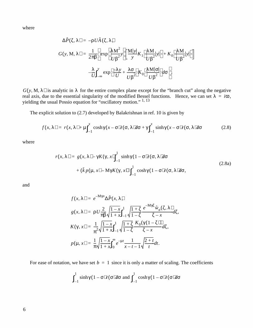
Similarly we have for the moment about the axis as,

(3.2)

where

Hence to calculate lift and moment we need to calculate two more constants namely,

We have again from (2.8a),

We are then left to find the twelve constants, , , , , , , ,

, , , and . It is difficult to obtain explicit formulas for these constants.

But since we are only interested in those terms of the order , we expand them in a power series

of M. Keeping terms up to , we obtain

and

x a=

M λ( ) x a–( )∆ P x λ,( ) xd1–

1

∫=

eMγx

x a–( ) r x( ) µ γ x σ–( )r σ( )cosh σd1–

x

∫+1–

1

∫=

γ γ x σ–( )r σ( )sinh σd1–

x

∫+ dx

1

M2k

---------- a– E0 r( ) E1 r( ) 1

M2k

----------eMγ

Ch r( )–+=

1Mγ-------- 1

1

k--- a–+

eMγ

Sh r( ),+

E1 r( ) xeMγx

r x( ) x.d1–

1

∫=

E0 r( ) and E1 r( ).

E0 r( ) E0 g( ) E0 K( )Sh r( )– kE 0 p( ) Mγ E0 K( )–[ ]Ch r( ),+=

E1 r( ) E1 g( ) E1 K( )Sh r( )– kE 1 p( ) Mγ E1 K( )–[ ]Ch r( ).+=

E0 g( ) E1 g( ) Sh g( ) Ch g( ) E0 p( ) E1 p( ) Sh p( )Ch p( ) E0 K( ) E1 K( ) Sh K( ) Ch K( )

M2

Mlog

M2

Mlog

L λ( ) L0 λ( ) M2

Mlog( )LM λ( )+= M λ( ) M0 λ( ) M2

Mlog( )MM λ( ),+=

10

where

(3.3)

and

.

Equation (3.3) is for a general class of lifting surfaces, in that the downwash function is arbitrary. Fora typical section we can express the downwash as

or

(3.4)

We ignore the initial conditions here since we will be interested only in the stability of the wing. Wecould also easily include control surfaces, but for simplicity we will not do so.

Plugging (3.4) into (3.3) we obtain:

(3.5)

L0 λ( ) 2ρU 1 σ+1 σ–------------- k 1 σ–( ) C k( )+[ ]wa σ λ,( ) σ,d

1–

1

∫–=

M0 λ( ) ρU1 σ+1 σ–------------- 1– 2ak– 1 2a+( )C k( )– 2 k 1 2a+( )+[ ]σ kσ2

–+{ }wa σ λ,( ) σ,d

1–

1

∫=

LM λ( ) ρU1 σ+1 σ–------------- k

33k

2+ C k( ) 2kC k( )2 σ k

32 k

2C k( )+[ ]–+{ }wa σ λ,( ) σ,d

1–

1

∫–=

MM λ( ) ρU1 σ+1 σ–------------- ak

3–{ 1 3a+( ) k

2C k( )– 1 2a+( ) kC k( )2

–1–

1

∫=

σ ak 3

1 2a+( ) k 2

C k( )+[ ]} wa σ λ,( )dσ+

C k( )K1 k( )

K1 k( ) K0 k( )+----------------------------------- Theodorsen function= =

wa x t,( ) h– t( ) x a–( )α t( )– Uα t( ), for x b,≤–=

wa λ( ) h– λ( ) x a–( )λα λ( )– U α λ( ).–=

L λ( ) πρU2b Lh k( ) h λ( )

b----------- Lα k( )α λ( )+ ,=

M λ( ) πρU2b

2Mh k( ) h λ( )

b----------- Mα k( )α λ( )+ ,=

11

where

(3.6)

Smilg and Wassermann15 defined the aerodynamic coefficients differently, they had

Lh k( ) k 2

2kC k( ) M2

Mlog k 4

2------ 2k

3C k( ) 2k

2C k( )2

+ + ,+ +=

Lα k( ) k ak 2

C k( ) 2 1 2a–( )k+[ ]+–=

M2

M k 3

2------

k 4

2------a C k( ) 2k

2 12--- 2a–

k 3

+ C k( )22k 1 2a–( )k

2+[ ]++–

,log+

Mh k( ) ak 2

1 2a+( )kC k( ) M2

Mlog 1 2a+( )k 2

C k( )2 12--- 2a+

k 3

C k( ) k 4

2------+ + a

,+ +=

Mα k( ) a12---–

k18--- a

2+

k 2

– C k( ) 1 2a12--- 2a

2–

k+ + M2

Ma2---k

3 a2

2-----k

4–

log+ +=

C+ k( )21 2a+( )k 1

2--- 2a

2–

k 2

+ C k( ) 12--- 2a+

k 2

2a2 k

3–+

.

L λ( ) π– ρU2bk

2Lh k( ) h λ( )

b----------- Lα k( ) 1

2--- a+

Lh k( )– α λ( )+

,=

M λ( ) π– ρU2b

2k

2Mh k( ) 1

2--- a+

Lh k( )–h λ( )

b-----------

=

Mαk12--- a+

– Lα k( ) Mh k( )+( ) 12--- a+

2Lh k( )+ α λ( )+

.

12

Here the coefficients are given by:

(3.7)

For , we have

Note: In the asymptotic expansions of the modified Bessel functions, we suppressed the dependence of on the reduced frequency . The dependence is such that the higher the value of , the smaller thevalue of M will need to be. However, for most aeroelastic calculations, we are only interested in the firstfew modes where is . In fact we have

. (3.8)

4. COMPARISON WITH PREVIOUS RESULTS

The definitions of the lift and moment coefficients in (3.6) are similar to those adopted by Possio,Dietze, and Timman. Timman’s lift and moment coefficients are defined for rotation about the midchord,

, hence his . These moment coefficients are different from equation (3.6) and Dietze’s values.For , figures 3–6 compare the aerodynamic coefficients in equation (3.6) with theircorresponding values found in Dietze and Timman. We also included the Prandtl-Glauert transformationof (3.6), i.e. all coefficients are divided by . As , the Prandtl-Glauert version will reach thecorrect steady state value. Upon close inspection we found that Dietze’s and were missing and respectively. When these errors are taken into account, our results show good agreementwith Dietze’s values. The differences between Dietze’s values and ours are all within 10 percent. Withthe adjustment of the rotation axis, the differences between Timman’s values and ours are also within10 percent, except at high reduced frequencies. At these high reduced frequencies Fettis found thatTimman’s values are erroneous.16 As for the moment coefficients, again Dietze left out some terms thereas well. When these errors are taken into account the difference between Dietze’s numbers and ours areagain within 10 percent (not shown).

Lh k( ) 12

k---C k( ) M

2Mlog k

2

2------ 2kC k( ) 2C k( )2

+ + ,+ +=

Lα k( ) 12---

1

k--- C k( ) 2

k 2

------2

k---+ M

2Mlog

k2---

k 2

4------ C k( ) 2

32---k+ C k( )2

22

k---++ + +

,+ + +=

Mh k( ) 12--- M

2Mlog

k 2

4------

k2---C k( )+

,+=

Mα k( ) 38---

1

k--- M

2Mlog

k4---

k 2

8------ C k( ) 1

2---

k2---++ +

.+ +=

a 12---–=

Lh k( ) k 2

Lh k( ), Lα k( ) k 2

Lα k( ), Mh k( ) k 2

Mh k( ), Mα k( ) k 2

Mα k( ).–=–===

γk( ) k

k 1<

γ Mλb

Uβ2---------- 1

β2-----λb

a∞------ 1

β2-----k∞ k∞ 1

M2

2-------+

k 1M

2

2-------+

≤≈= = =

a 0= LαM 0.5=

β k 0→Lh Lα k

2–

k2

2⁄–

13

Figure 3. Lift coefficient due to plunge motion as a function of reduced frequency with (real part).

Figure 4. Lift coefficient due to plunge motion as a function of reduced frequency with (imaginary part).

k( ) M 0.5=

k( ) M 0.5=

14

Figure 5. Lift coefficient due to pitch motion as a function of reduced frequency with (real part).

Figure 6. Lift coefficient due to pitch motion as a function of reduced frequency with (imaginary part).

k( ) M 0.5=

k( ) M 0.5=

15

For the case where figures 7–10 compare results from equation (3.7) with those thatbelong to Fettis2 and Blanch11 whenever they follow Smilg and Wassermann notations. Blanchemployed Reissner’s method to calculate the aerodynamic coefficients, whereas Fettis approximatedPossio’s equation in obtaining his results. It is uncanny that the values are within a few hundredths ofeach other. Our numbers compare reasonably well with theirs for and shown infigures 8 and 9 respectively. The differences are close to 15 to 20 percent. However, for and

, there is nearly a 60-percent difference between our results and theirs. For this particular Machnumber Fettis’ values agreed with Dietze’s when he took into account Dietze’s missing factorsmentioned earlier. There were some difficulties in the convergence of Dietze’s iteration scheme for sucha high Mach number. Fettis bypassed these difficulties by approximating Possio’s integral equation witha polynomial. He expanded the kernel function in a power series of after he had removed theincompressible part. On the other hand, Blanch followed Reissner’s method of expansions in terms of theMathieu functions. Hence, their approximations are no longer valid for large Mach numbers and largereduced frequencies. Neither Fettis nor Blanch indicated how many terms should be taken in theirexpansions or what the limiting values are for the Mach number or the reduced frequency in theirapproximations. Our results are also approximations, but they are analytic rather than numericalapproximations. If our approximations are good enough for and they should be goodenough for and as well. The differences are even greater in the moment coefficients.These differences are 60-percent and beyond (not shown). Just as with lift coefficients, we simply cannotconclude which approximation is better. From (3.7) it follows that

which is a formula derived by Fettis in reference 15. This relation is exact and was derived analyticallybased solely on the kinematics of the airfoil and the existence and uniqueness of the solution to the Possioequation. Overall, for and our approximations are in good agreement with previoustabulated values.

Figure 7. Lift coefficient due to plunge motion as a function of reduced frequency with (real part).

M 0.7,=

Im Lh[ ] Re Lα[ ]Re Lh[ ]

Im Lα[ ]

k

Im Lh[ ] Re Lα[ ],Re Lh[ ] Im Lα[ ]

Mh k( ) Lα k( )+ 11

k---+

Lh k( ),=

M 0.7< k 1,<

k( ) M 0.7=

16

Figure 8. Lift coefficient due to plunge motion as a function of reduced frequency with (imaginary part).

k( ) M 0.7=

Figure 9. Lift coefficient due to pitch motion as a function of reduced frequency with (real part).

k( ) M 0.7=

17

Figure 10. Lift coefficient due to pitch motion as a function of reduced frequency with (imaginary part).

5. APPLICATION TO FLUTTER ANALYSIS

A main motivation for calculating the lift and moment in unsteady aerodynamics is for use inaeroelastic stability analysis—flutter speed calculations. In this section, we calculate the “aeroelasticmodes” (see reference 13, p. 550) of a wing with a large aspect ratio and demonstrate the simplicity andthe ease of utility of the explicit lift and moment formulas found in section 3. We will also see the needfor the Laplace transforms of lift and moment as opposed to the “oscillatory motion” values whencalculating these “aeroelastic modes.”

We illustrate this with the continuum model of Goland17 for bending-torsion flutter for a uniformcantilever wing. The flutter speed has been calculated in references 17 and 18 for the incompressiblecase. Here we shall use our formulas to calculate the aerodynamic loading in the subsonic compressiblecase.

The dynamic equation for the wing is given as

(5.1)

k( ) M 0.7=

m∂2

h y t,( )∂t

2-------------------- Sy

∂2α y t,( )∂t

2--------------------- EI

∂4h y t,( )∂y

4-------------------- L y t,( ),–=+ +

I y∂2α y t,( )

∂t2

--------------------- Sy∂2

h y t,( )∂t

2-------------------- GJ

∂2α y t,( )∂y

2---------------------–+ M y t,( ),=

0 t , 0 y l,≤ ≤≤

18

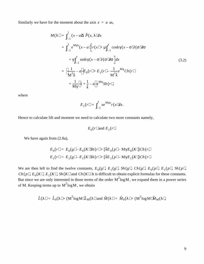
with boundary conditions of,

Goland used the lift and moment of an infinitely spanned wing, but in actuality due to their dependenceon h and , the lift and moments in (5.1) do depend on y. For a wing with a sufficiently large aspect ratio,one can argue that the lift and moment can be written as the sum of the lift and moment of the infinitelyspanned wing with a correction term that goes to zero as .19

Therefore, we proceed by taking the Laplace transform of equation (5.1) and denote the derivativewith respect to y by superprime. We then have

(5.2)

with boundary conditions:

.

These equations yield the “aeroelastic” modes. The main point here is that we need given by (3.6), ( is not purely imaginary). We may then proceed to calculate the real part of theaeroelastic mode corresponding to the first torsion mode, following reference 18, where the onlydifference is that the aerodynamics is restricted to the incompressible case, as in Goland. Figures 11and 12 plot the real part of as a function of U, for the compressible as well as the incompressible case,at two different elevations. The flutter speed differs little from the incompressible case prior to flutter,even though the damping is higher initially. Tables 1 and 2 summarize the wing parameters and theflutter analysis. All of the reduced frequencies and Mach numbers at flutter condition are well within therange of validity of our approximation.

h 0 t,( ) ∂h 0 t,( )∂y

------------------ α 0 t,( ) 0, and ∂2

h l t,( )∂y

2-------------------

∂3h l t,( )∂y

3-------------------

∂α l t,( )∂y

----------------- 0.= = == = =

α

y ∞→

mλ2h y λ,( ) Syλ2α y λ,( ) EIh″″ y λ,( )+ + L y λ,( ),–=

I yλ2α y λ,( ) Syλ2h y λ,( ) GJ α″ y λ,( )–+ M y λ,( ),=

0 y l≤ ≤

h 0 λ,( ) h 0 λ,( ) α 0 λ,( ) h″ l λ,( ) h′′′ l λ,( ) α'ˆ l λ,( ) 0= = = = = =

L y λ,( ) M y λ,( ),λ

λ

19

Figure 11. as a function of air speed: Goland case at sea level.

Figure 12. as a function of air speed: Goland case at 20,000 ft.

Re λ[ ]

Re λ[ ]

20

Table 1. Parameters of the wing: Goland case.

Parameters Values

m 0.746 slug/ft

Sy 0.447 slug/ft/ft

Iy 1.943 slug/ft2/ft

EI 23.6 × 106 lb ft

GJ 2.39 × 106 lb ft

a –1/3

l 20 ft

b 3 ft

Table 2. Flutter analysis of the wing: Goland case.

Sea level 20 K ft above sea level

Uf (ft/sec) kf Mf Uf (ft/sec) kf Mf

Incompressible 447 0.47 ∞ 574 0.36 ∞Compressible 446 0.46 0.40 574 0.35 0.55

21

6. CONCLUDING REMARKS

For application to aeroelastic analysis in the subsonic compressible regime, the current reliance ontabulated calculations of aerodynamic influence coefficients is cumbersome. In this paper, closed-formformulas of lift and moment coefficients are obtained based on the recent solution of the Possio equationby Balakrishnan.

For a Mach number less than 0.7 and reduced frequencies less than one, the closed-form formulas oflift and moment coefficients derived in this paper are within 10 percent of previous numerical results.As the Mach number gets closer to 0.7 and beyond, all methods of approximation fail. However, for sucha high Mach number the aerodynamic flow is close to the transonic regime.

Numerical calculations are shown to be consistent with extant work. The ease of use of theseformulas is demonstrated in the flutter analysis illustrated. No longer is there a need for “table look up” ofaerodynamic coefficients in an iterative process of root finding.

REFERENCES

1. Possio, Camillo, “Aerodynamic Forces on an Oscillating Profile in a Compressible Fluid at SubsonicSpeed.” Aerotecnica, vol. 18, 1938, pp. 441–458.

2. Dietze, F., “The Air Forces of the Harmonically Vibrating Wing at Subsonic Velocity (PlaneProblem),” Parts I and II. U.S. Air Force translations, F-TS-506-RE and F-TS-948-RE, 1947.Originally appeared in Luftfahrt-Forsch, vol. 16, no. 2, 1939, pp. 84–96.

3. Fettis, Henry E., “Tables of Lift and Moment Coefficients for an Oscillating Wing-AileronCombination in Two-Dimensional Subsonic Flow,” Air Force Technical Report 6688, 1951.

4. Haskind, M. D., “Oscillations of a Wing in a Subsonic Gas Flow,” Brown University translation,A9-T-22, 1948. Originally appeared in Prikl. Mat. i Mekh. vol. XI, no. 1, 1947, pp. 129–146.

5. Reissner, Eric, On the Application of Mathieu Functions in the Theory of Subsonic CompressibleFlow Past Oscillating Airfoils, NACA TN-2363, 1951.

6. Timman, R., A. I. van de Vooren, and J. H. Greidanus, “Aerodynamics Coefficients of an OscillatingAirfoil in Two-Dimensional Subsonic Flow,” Journal of the Aeronautical Sciences, vol. 18, no. 12,December 1951, pp. 797–802.

7. Watkins, C. E., H. L. Runyan, and D. S. Woolston, On the Kernel Function of the Integral EquationRelating the Lift and Downwash Distributions of Oscillating Finite Wings in Subsonic Flow, NACAReport 1234, 1955.

8. Albano, E. and W. P. Rodden, “A Doublet-Lattice Method for Calculating Lift Distribution onOscillating Surfaces in Subsonic Flows,” AIAA Journal, vol. 7, no. 2, February 1969, pp. 279–285.

22

9. Rodden, W. P., “The Development of the Doublet-Lattice Method,” Proceedings of the AIAAInternational Forum on Aeroelasticity and Structure Dynamics, Rome, Italy, 1997.

10. Balakrishnan, A. V., Unsteady Aerodynamics-Subsonic Compressible Inviscid Case, NASACR-1999-206583, August 1999.

11. Blanch, G., “Tables of Lift and Moment Coefficients for Oscillating Airfoils in SubsonicCompressible Flow,” National Bureau of Standards Report 2260, 1953.

12. Küssner, H. G., “General Airfoil Theory,” NACA TM-979, June 1941. Originally: “AllgemeineTragflächentheorie.” Luftfahrt-Forsch, vol. 17, no. 11–12, December 1940, pp. 370–378.

13. Bisplinghoff, Raymond L., Holt Ashley, and Robert L. Halfman, Aeroelasticity, Dover Edition,New York, 1996.

14. Küssner, H. G., and L. Schwarz, The Oscillating Wing with Aerodynamically Balanced Elevator,NACA TM-991, 1941. Translated from Luftfahrt-Forsch, vol. 17, no. 11–12, December 1940,pp. 337–354.

15. Smilg, Benjamin and Lee S. Wassermann, “Applications of Three-dimensional Flutter Theory toAircraft Structures,” Air Force Technical Report 4798, 1942.

16. Fettis, Henry E., “Reciprocal Relations in the Theory of Unsteady Flow Over Thin Airfoil Sections,”Proceedings of the Second Midwestern Conference on Fluid Dynamics, Columbus, Ohio, 1952,pp. 145–154.

17. Goland, M., “The Flutter of a Uniform Cantilever Wing,” Journal of Applied Mechanics, vol. 12,no. 4, December 1945, pp. A197–A208.

18. Balakrishnan, A. V., “Aeroelastic Control With Self-Straining Actuators: Continuum Models,”Proceedings of SPIE Smart Structures and Materials Conference 1998: Mathematics and Control inSmart Structures, vol. 3323, San Diego, California, July 1998, pp. 44–54.

19. Reissner, E., Effect of Finite Span on the Airfoil Distributions for Oscillating Wing-I, Theory, NACATN-1494, March 1947.

REPORT DOCUMENTATION PAGE Form ApprovedOMB No. 0704-0188

Public reporting burden for this collection of information is estimated to average 1 hour per response, including the time for reviewing instructions, searching existing data sources, gathering andmaintaining the data needed, and completing and reviewing the collection of information. Send comments regarding this burden estimate or any other aspect of this collection of information,including suggestions for reducing this burden, to Washington Headquarters Services, Directorate for Information Operations and Reports, 1215 Jefferson Davis Highway, Suite 1204, Arlington,VA 22202-4302, and to the Office of Management and Budget, Paperwork Reduction Project (0704-0188), Washington, DC 20503.

1. AGENCY USE ONLY (Leave blank) 2. REPORT DATE 3. REPORT TYPE AND DATES COVERED

4. TITLE AND SUBTITLE 5. FUNDING NUMBERS

6. AUTHOR(S)

8. PERFORMING ORGANIZATION REPORT NUMBER

7. PERFORMING ORGANIZATION NAME(S) AND ADDRESS(ES)

9. SPONSORING/MONITORING AGENCY NAME(S) AND ADDRESS(ES) 10. SPONSORING/MONITORING AGENCY REPORT NUMBER

11. SUPPLEMENTARY NOTES

12a. DISTRIBUTION/AVAILABILITY STATEMENT 12b. DISTRIBUTION CODE

13. ABSTRACT (Maximum 200 words)

14. SUBJECT TERMS 15. NUMBER OF PAGES

16. PRICE CODE

17. SECURITY CLASSIFICATION OF REPORT

18. SECURITY CLASSIFICATION OF THIS PAGE

19. SECURITY CLASSIFICATION OF ABSTRACT

20. LIMITATION OF ABSTRACT

NSN 7540-01-280-5500 Standard Form 298 (Rev. 2-89)Prescribed by ANSI Std. Z39-18298-102

Aerodynamic Lift and Moment Calculations Using a Closed-FormSolution of the Possio Equation

WU 529 50 04 T2 RR 00 000

Jensen Lin and Kenneth W. Iliff

NASA Dryden Flight Research CenterP.O. Box 273Edwards, California 93523-0273

H-2374

National Aeronautics and Space AdministrationWashington, DC 20546-0001 NASA/TM-2000-209019

In this paper, we present closed-form formulas for the lift and moment coefficients of a lifting surface in two-dimensional, unsteady, compressible, subsonic flow utilizing a newly developed explicit analytical solution ofthe Possio equation. Numerical calculations are consistent with previous numerical tables based on seriesexpansions or ad hoc numerical schemes. More importantly, these formulas lend themselves readily to flutteranalysis, compared with the tedious table-look-up schemes currently in use.

Aeroelasticity, Lift and moment coefficients, Possio equation, Subsonicaerodynamics, Unsteady Aerodynamics

A03

28

Unclassified Unclassified Unclassified Unlimited

April 2000 Technical Memorandum

Jensen Lin, University of California, Los Angeles, California and Kenneth W. Iliff, Dryden Flight ResearchCenter, Edwards, California. Part of NASA DFRC grant NCC2-374 with UCLA.

Unclassified—UnlimitedSubject Category 02

This report is available at http://www.dfrc.nasa.gov/DTRS/