INSTITUTO TECNOLÓGICO DE AERONÁUTICA

DIVISÃO DE ENGENHARIA MECÂNICA-AERONÁUTICA

Internship Report

Aerodynamic Analysis for Control and

Simulation of Unmanned Aerial Vehicles

Author: Supervisors: Roderik Kuin Prof. Luiz Carlos S. Góes (ITA) Dr. Roberto Gil Annes da Silva (IAE) Prof H.W.M.Hoeijmakers (UTWENTE)

Roderik Kuin s0166634

INSTITUTO TECNOLÓGICO DE AERONÁUTICA- DIVISÃO DE ENGENHARIA MECÂNICA-AERONÁUTICA

Prof. Luiz Carlos S. Góes

Sao Jose dos Campus – Brasil

October 2012 – January 2013

University of Twente, CTW, EFD, Prof H.W.M. Hoeijmakers

Introduction

This research project is focused on the aerodynamic modeling of unmanned aerial vehicles (UAV) and

its application to determine the aircraft aerodynamic characteristics. The aerodynamic modeling

procedure of the UAV is based on the vortex lattice method (VLM). The goal is the computation of

the aerodynamic stability and control derivatives for composing the flight vehicle equations of

motion. The vortex lattice method code that will be used is the Tornado VLM Toolkit, a MATLAB

based freeware program developed at KTH- Sweden. The aerodynamic (stability) derivatives shall be

validated by comparing the calculated derivatives with the corresponding aerodynamic derivatives

identified from experimental flight data. The unmanned aerial vehicles that is used for this research

is called Vector-P. A picture of the aircraft is shown below.

Figure 1 - UAV-Vector P

Table of Contents 1. Theory .............................................................................................................................................. 6

1.1 Aerodynamic derivatives ......................................................................................................... 6

1.2 Vortex Lattice Method ............................................................................................................ 7

1.2.1 Bio-Savart law .................................................................................................................. 9

2. CFD Calculations of the Aerodynamic Derivatives Vector-P ......................................................... 10

2.1 Tornado ................................................................................................................................. 10

2.2 Vector P Specifications .......................................................................................................... 12

2.3 Modelling Vector-P ................................................................................................................ 14

2.3.1 Modelling the wing ............................................................................................................... 14

2.3.2 Modelling the horizontal tail ................................................................................................ 16

2.3.3 Modeling the vertical tail ..................................................................................................... 17

2.3.4 Modeling the fuselage .......................................................................................................... 18

2.4 Number of panels .................................................................................................................. 19

2.5 Results ................................................................................................................................... 21

3. CFD Calculations of the Aerodynamic Derivatives Telemaster ..................................................... 23

3.1 Dimensions of the Telemaster. ............................................................................................. 23

3.2 Modelling Telemaster............................................................................................................ 25

3.2.1 Modelling the wing ........................................................................................................ 25

3.2.2 Modeling the horizontal tail .......................................................................................... 26

3.2.3 Modeling the vertical tail .............................................................................................. 27

3.2.4 Modeling the fuselage ................................................................................................... 28

3.3 Number of Panels .................................................................................................................. 30

3.4 Results ................................................................................................................................... 31

4. Comparing Test Data with CFD Results ......................................................................................... 33

4.1 Comparison CFD results with flight testing ........................................................................... 33

4.1.1 Method of flight testing ................................................................................................ 33

4.2 Equations of Motion .............................................................................................................. 36

4.2.1 Forces ............................................................................................................................ 37

4.2.2 Moments ....................................................................................................................... 38

4.2.3 Kinematic relations ........................................................................................................ 39

4.3 Comparison Tornado with flight test data ............................................................................ 40

4.3.1 Vector-P ......................................................................................................................... 40

4.3.2 Telemaster ..................................................................................................................... 40

4.4 The effects in the difference in the aerodynamic coefficients of Tornado and flight tests of

the Vector-P....................................................................................................................................... 42

5. Conclusion ..................................................................................................................................... 45

Appendix A ............................................................................................................................................ 46

References ............................................................................................................................................. 47

1. Aerodynamic Theory

In this part of the report, the meaning of the aerodynamic derivatives is explained. After that the

theory behind the Vortex Lattice Method is explained and how it can modulate an airfoil. In order to

understand the theory of the Vortex Lattice Method it is necessary to know Biot-Savart law.

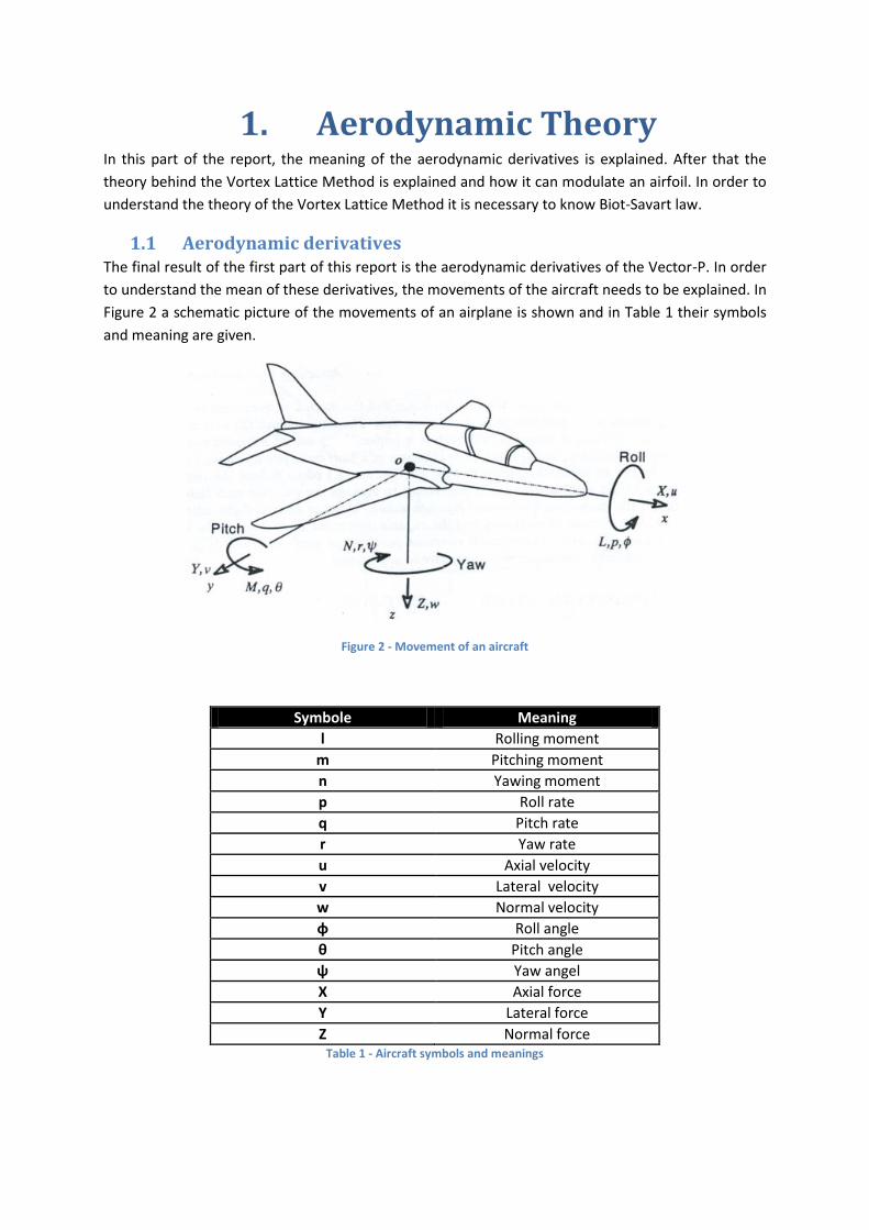
1.1 Aerodynamic derivatives The final result of the first part of this report is the aerodynamic derivatives of the Vector-P. In order

to understand the mean of these derivatives, the movements of the aircraft needs to be explained. In

Figure 2 a schematic picture of the movements of an airplane is shown and in Table 1 their symbols

and meaning are given.

Figure 2 - Movement of an aircraft

Symbole Meaning

l Rolling moment

m Pitching moment

n Yawing moment

p Roll rate

q Pitch rate

r Yaw rate

u Axial velocity

v Lateral velocity

w Normal velocity

φ Roll angle

θ Pitch angle

ψ Yaw angel

X Axial force

Y Lateral force

Z Normal force Table 1 - Aircraft symbols and meanings

The aerodynamic derivatives that are searched for, follow from the lift coefficient (CL), drag

coefficient (CD), side force coefficient (CY) and the moment coefficients along the x-,y-, and z-axis (Cl,

Cm, Cn ).This coefficients are defined as:

where q is the dynamic pressure, c is chord and S span of the wing.

The aerodynamic derivatives that are searched for follow from the functions of the six coeffincent:

( )

( )

( )

( )

( )

( )

where , are the derivatives with respect changes of the evaluator, ruder, flap and

aileron.

1.2 Vortex Lattice Method The Vortex Lattice Method is a method that is used to make a numerical model of lifting surface like

wings. It models the wing as an infinitely thin sheet of discrete vortices to compute lift and induced

drag.

The vortex lattice method is based on the theory of an ideal flow, also known as a potential flow. An

ideal flow is a simplification of the real flow experienced in nature. The following assumptions are

made regarding the problem in the Vortex Lattice Method:

The flow field is incompressible, inviscid and irrotational

The lifting surfaces are thin

The angle of attack is small.

With the assumptions above it can been shown that there is a function φ such that

Φ is called the velocity potential. The velocity potential holds the Laplace equation

The Laplace equation is a second order linear equation and therefore it is allowed to use the principle

superposition.

Consider a part of a finite wing as shown in Figure 3. A panel is defined by the dashed lines on the

wing, where l is the length of the panel in the free stream direction. A horseshoe vortex abcd of

strength is place on the panel. The segment bc of the horseshoe is a distance l/4 from the front of

the panel. A control point is placed on the centerline ¾ l from the front of the panel. The velocity

induced at an arbitrary point P by the horseshoe, can be determined by applying Biot-Savart law on

each of the three vortex filaments of the horseshoe. The Biot-Savart law will be explained late in this

paragraph.

Figure 3 - A horseshoe vortex on a part of a wing

Consider now the entire wing to be covered by a finite number of panels. On every panel a

horseshoe vortices is placed. For example the panel behind the leading, there is the horseshoe vortex

abcd. On the panel behind it, there is the horseshoe vortex aefd. On the next panel there is

horseshoe vortex aghd ect. This is shown in Figure 4. The entire wing is now covered by a lattice of

horseshoe vortices, each of a different unknown strength .

Figure 4 - Vortex lattice system on a finite wing

The central problem of the Vortex Lattice Method is to determine the strength of the vortices such

that the normal component of de free stream velocity is zero. The flow is than tangent to the lifting

surface. For each panel this condition is applied on the control point. The normal velocity component

exists of a free stream component and an induced flow component. This induced component is a

function of all the strengths of all the horseshoe vortices on the wing. For each panel an equation can

be set up which is a linear combination of the effects of all the panels. When applying the flow

tangency on all the control points, a system of simultaneous algebraic equations results which can be

solved for the unknown . The algebraic set of equations is shown below.

[

] [

] [

]

( )

The matrix [A] is the aerodynamic influence matrix where the induced velocity of each vortex on

each panel is collected and Γ is the strength of each vortex. When the above set of equations is

solved the aerodynamic forces can be determined as follows:

( )

1.2.1 Bio-Savart law

Consider a vortex filament with strength Γ as shown in Figure 5. A part the filament, dl, induces a

flow field in the surrounding space, for example at the arbitrary point P. If the distance from dl to the

P in the surrounding space is r, then the segment dl induces a velocity at P equal to

| |

This is called Biot-Savart law.

Figure 5 - Vortex filament

2. CFD Calculations of the

Aerodynamic Derivatives Vector-P In this chapter the Matlab program Tornado, which will be used to make a numerical model of

Vector-P, will be explained. The dimension of the unmanned aircraft, Vector P will be determined

and that will be used as an input in Tornado. All the steps that were made in order to make the

numerical model will be explained. At last the results, output of Tornado, will be shown and

discussed.

2.1 Tornado Tornado is a 3D-vortex lattice program with flexible wake and can be used for a variety of tasks.

Tornado is based on the standard vortex lattice theory as described earlier in this report. The wake

coming of the trailing edge of the lifting surface is flexible and changes from shape according to

different flight conditions. The classical horse-shoe, which is explained earlier, is in this program

replaced by a “vortex-sling”. The difference between a horse-shoe and a vortex-sling is that the legs

of the vortex-sling are flexible and consist of seven vortices of equal strength in stead off three. This

is shown in Figure 6.

Figure 6 - Vortex-sling VS. Horse shoe

The outputs of the program are 3D forces acting on each panel, aerodynamic coefficients in both

body and wind axis and stability derivatives with respect to the angle of attack, angle of sideslip,

angular rates and rudder deflections. The aerodynamic derivatives are calculated by using a centrals

difference calculation using the selected state of the aircraft and disturbing it by 0.5 degrees. So for

an arbitrary aerodynamic coefficient, it is calculated as follows

In order to model the Vector-P in Tornado a lot settings are needed to be filled in. Therefore the

types of settings of Tornado are explained below.

Coordinate system: a Cartesian coordinate system is used within the programme Tornado. The X-axis

is along the aircraft body and increasing in the direction of the tail. The Y-axis is aligned positive out

through the starboard wing in span wise direction. The Z-axis is right-hand perpendicular to the X-

and the Y-axis, where the positive axis is upwards.

Span: the span that is required to be filled in is the semi span of each partition. It is the distance from

the innermost to the outermost part of each partition. The sum of the semi spans of all the partitions

is the semi span of the entire wing.

Taper: with taper the programme means the tapper ratio. The taper ratio is defined as:

Sweep: with sweep the programme means the swept angle of each partition. The swept angle is the

angle between the quarter chord line and the Y-axis.

Chamber: The chamber lines that Tornado uses are from the NACAXXXX series. For each partitions of

the wing both the inner and the outer chamber must be specified.

Dihedral: The dihedral angle is the angle between the XY-plane and the quarter chord line.

Twist: the partition twist is defined as the angle between the tip chord of the partition and the root

chord of the wing.

Symmetry: when there is symmetry there is a mirror of the partition in the XY-pane. Tornado work

with a Boolean operator, 1 is yes and 0 is no.

Root chord: The root chord has to be specified for each wing. For the partitions the root chord will be

defined by the first partition root chord and the taper ratio.

Flaps: the programme will see flaps and aileron as flaps but that have to be modelled separately

because they have different functions. See flaps symmetry

Flap symmetry: if there is symmetry of a partition of the wing which has a flap (flap or aileron) the

programme needs to flaps deflect symmetrically. For example, whether or not the starboard and the

port flap go up or down at the same time. This is true for flaps and evaluators, but not for ailerons.

To fill the settings, Tornado again uses a Boolean operate.

Flap chord fraction of the local wing chord: If there is a flap the chord of the flap needs to be defined.

This is done by the fraction of the flap chord with respect to the local wing chord.

Panels: For each partition a number of panels can be chosen in the chord wise as in span wise

direction. The chosen of the number of panels will be explained later in this report.

2.2 Vector P Specifications There is not much known about the Vector P. The specifications of the aircraft that are known are

listed in the table below. These specifications are from the factory where Vector-P was fabricated.

Unmanned Aerial Vector-P Specifications

Wingspan 2.6 m

Fuselage Length 1.525 m

Max Speed 185 Km/h

Engine 3 W 2-stroke reverse rotation gasoline engine. Options range from 2.48 to 4W, quoted on request.

Max Range 775 Km, depending on fuel on board

Cruise Speed 129 Km/h

Max Altitude 3 Km

Max Endurance 6 hours depending on fuel and payload on board

Max Takeoff Weight

34 Kg

Empty Weight 23 Kg

Max Fuel 12.3 liters

Fuel Per Hour 2.3 liters

Landing Speed 74 Km/h

Max Payload Weight

11.3 Kg, with fuel for one hour

Payload Vol. (Internal)

(225 x 225 x 685) mm

Payload Power (typ) 18.5 +2.5/-1 VDC @ 2.5 A, 6 Ah, distributed

Max Comm. Range 62 Km Line of Sight

Takeoff & Landing Manual RC Control (spread spectrum), runway < 150m depending on surface and Takeoff Weight

Table 2- Vector P Specifications

As can been seen in the table above, there is not much information about the dimensions and the

aerodynamics of the airplane. In order to make a numerical model, all the dimensions and the

profiles of the wing and the tail need to be known. All the useful dimensions are measurement. The

profile of the wing and the tail are an approximation of a NACA profile. This is done by measuring the

chord of the wing and the maximum thickness. To check whether the approximation was accurate, a

mold was made of the approximated profile. If the mold fitted nicely around the airfoil, the

approximation is assumed to be good enough. For the wing, the airfoil is approximated to have a

NACA 4412 profile. For the horizontal and vertical tail, the airfoil is approximated to be a NACA 0010

profile. The dimensions of the wing and the tail are shown in the pictures below.

Figure 7- Top view of Vector-P. Dimensions in mm

Figure 8 - vertical tail and horizontal tail, dimensions in mm

The exact shape of the Vector-P cannot be modelled. The flaps of the tails are not entirely straight,

some corners are cut off. It is not possible to model the flaps like that in Tornado, therefore the flaps

will be modelled as if they are fully rectangular. The wing is not exactly an exact rectangle either. The

corners are not sharp edges but there are round and that is also not possible to model in Tornado.

Figure 9 - Fuselage of the Vector-P

As mentioned before, Tornado approximated the lifting surfaces by pretending that they are very

thin. The fuselage is not thin but it needs to be modelled because it has influences on the flow

around the wings. To model these influence, it is chosen to model the fuselage as to two thin plats,

one horizontally and one vertically. The dimensions of the fuselage are shown in Figure 9. The front

part of the fuselage is round, it has an oval shape. This is impossible to model in Tornado, therefore

the nose of the fuselage is approximated for a triangular shape.

For a good numerical model it is also important to know where the centre of gravity is located. The

centre of gravity plays an important role with respect to the stability of the aircraft. The location of

the centre of gravity depends on where the electronic equipment is placed in the fuselage. This is not

every time exactly the same therefore the centre of gravity is approximated to be in the centre of the

fuselage 0.1 meter behind the leading edge of the wing.

The tail of the Vector-P is connected to the wing with two bars. The two bars have a small diameter

and therefore it is assumed that it has minimal effect on the flow. With this assumption it is chosen

not to model the bars in Tornado.

2.3 Modelling Vector-P To model the Vector-P in Tornado, each part, like the wing, tail and fuselage needs to be model

separately and all have different setting. In this part of the Chapter the settings for each part of the

Vector-P will be discussed separately

2.3.1 Modelling the wing

The first part of Vector-P that is modelled in Tornado is the wing. The wing is in the model divided up

into different partitions in span wise direction. Each partition will have different kind of settings, this

will be specified later in this the report. First the wing span is divided into 4 different partitions. The

first partition is the part of the wing which starts at the root chord until the beginning of the flap. The

second partition is the whole span of the flaps. The third partition is the whole span of the aileron

and the last partition is the tip of the wing, which is from the end of the aileron until the end of the

wing. This would be the corrected to model a single wing but in this case a tail of the airplane needs

to be modelled as well. This brings a numerical problem. When the wing and the tail are divided into

panels, the panels of the wing and tail should be in the same line in span wise direction. In other

words, all the spanwise divisions of the tail must be aligned with those of the wing. See Figure 10. If

this is violated it is possible that a vortex line of the wing will shed a control point on the tail. This

would make the aerodynamic influence matrix singular which would result into wrong results.

Figure 10 – span wise alignment

In order to fulfill the requirement that the span wise divisions of the tail are aligned with the span

wise divisions of the wing, an extra partition in the wing is needed. The span of the tail is smaller than

the span of the wing form the root chord until the beginning of the flap. Therefore the wing needs an

extra partition from the end of the span of the tail until the beginning of the flap.

To complete the model of the wing in Tornado all that settings that are explained earlier in this

report are filled in. In Figure 11 the partitions of the wing are shown and in Table 3 all settings that

have been explained are given.

Figure 11 - Model of the wing

Wing No. Partitions 5

Partitions 1 Partitions 2 Partitions 3 Partitions 4 Partition 5

Symmetric 1 1 1 1 1

Apex coordinates

(x,y,z)

0 0.115 1

Base Chord (m)

0.4451

Half span (m) 0.225 0.04616 0.33369 0.481 0.09

Sweep (rad) 0 0 0 0 0

Dihedral (rad) 0 0 0 0 0

Taper 1 1 1 1 1

Airfoil 4412 4412 4412 4412 4412

Twist (rad) 0 0 0 0 0

Flapped 0 0 1 1 0

Chord flap 0 0 0.1603 0.1603 0

Flaps deflect symmetric

0 0 1 0 0

Table 3 - Wing settings

From Table 3 it can be seen that the base chord is only given for the first partitions of the wing. It is

not necessary to know the rest of the chords, because Tornado will calculated that with setting of the

taper ratio, half span and the length of the root chord.

2.3.2 Modelling the horizontal tail

To model the tail of the Vector-P, the number of partitions has to be decided first. In the section

above, there has been explained that the span wise divisions of the tail must be aligned with the

span wise divisions of the wing. For the tail, there is a similar requirement, namely the span wise

division of the horizontal fuselage needs to be aligned with the span wise divisions of the tail.

Therefore the tail is divided into two partitions. The first partition is exactly the half of the width of

the fuselage (because of symmetry) and the second partition is the rest of the tail. In Figure 12 the

partitions of the tail are shown and in Table 4 all settings that have explained are given.

Figure 12 - Model wing + horizontal tail, top view

Horizontal tail No. Partitions 2

Partitions 1 Partitions 2

Symmetric 1 1

Apex coordinates (x,y,z) 1.4386 0 0

Base Chord (m) 0.25434

Half span (m) 0.115 0.225

Sweep (rad) 0 0

Dihedral (rad) 0 0

Taper 1 1

Airfoil 0010 0010

Twist (rad) 0 0

Flapped 0 0

Chord flap 0.2949 0.2949

Flaps deflect symmetric 1 1 Table 4 - Settings of the horizontal tail

2.3.3 Modeling the vertical tail

For the vertical tail there is only one partitions needed. The schematic view of vertical tail can be

seen below.

Figure 13- Model of the vertical tail, side view

In Figure 13 a schematic view of the vertical tail is given. It can be seen that the chord of the flap

decreases in span wise direction. This is because the fraction of the flap is defined as:

In Tornado the fraction stays the same and because the tail has a tapper ratio less than one, the

chord of the flap decreases in the model. In the real plane the chord of the flap stays the same in

span wise direction. Unfortunately Tornado cannot model this and therefore it is a limitation of the

program.

Settings Vertical Tail No. Partitions 1

Partition 1

Symmetric 1

Apex coordinates (x,y,z) 1.439 0.34 0

Base Chord (m) 0.249

Half span (m) 0.341

Sweep (rad) 0.1594

Dihedral (rad) 1.57

Taper 0.7

Airfoil 0010

Twist (rad) 0

Flapped 1

Chord flap 0.281

Flaps deflect symmetric 0 Table 5 – Settings of the vertival tail

The calculation of the swept angle is shown in Appendix A.

2.3.4 Modeling the fuselage

The horizontal part and the vertical part of the fuselage both exist of 1 partition. It is important for

the fuselage that the panels of the fuselage are well connected to the panels of the two wings and

with each other. To fulfill this, the fuselage is modeled as three “lifting surface” behind each other

for the horizontal part as well as for the vertical part. The first lifting surface is in front of the two

wings, the second between the two wings and the third lifting surface behind the two wings. The

model and the settings are shown in below.

Figure 14 - Model of Vector-P, top view

Figure 15 - Model of Vector-P, side view

Fuselage horizontal Fuselage vertical

Wing 1 Wing 2 Wing 3 Wing 1 Wing 2 Wing 3

Symmetric 1 1 1 0 0 0

Apex coordinates

(x y z)

-0.85 0 0 0 0 0 0.4451 0 0 -0.85 0 -0.165

0 0 -0.165 0.4451 0 -0.165

Base Chord(m)

0.85 0.4451 0.0449 0.85 0.4451 0.0449

Half span (m) 0.115 0.115 0.115 0.280 0.280

Sweep(rad) 0 0 0 0.359 0 0

Dihedral (rad)

0 0 0 1.57 1.57 1.57

Taper 1 1 1 0.835 1 1

Airfoil 0 0 0 0 0 0

Twist (rad) 0 0 0 0 0 0

flapped 0 0 0 0 0 0

Chord flap 0 0 0 0 0 0

Flaps deflect symmetric

0 0 0 0 0 0

Table 6 - settings of the fuselage

In Table 6 the numbers of the wings are counted from the noise of the aircraft in the direction of the

tail. The calculation of the dihedral angle is shown in Appendix A.

2.4 Number of panels The total aircraft is now modeled in tornado. The only thing that needs to be set in order to run

Tornado, is the number of panels. This is an important setting because a too low number of panels

will give an inaccurate result and too many panels results in a long calculation time. To decide how

many panels should be used, there has been looked at two different aerodynamic derivatives. One

derivative that is most sensitive to the deviation of the number of panels in the XY plane and the

second derivative that is most sensitive to the deviation of the number of panels in the XZ-plane. The

XY-plane and the XZ-plane are the only planes where the number panels can change. The most

sensitive derivative in the XY plane is Clα and in the XZ plane it is Cyβ . The correct number of panels

that should be used for the model is where Clα and Cyβ have converged to a result.

It is not possible just to a guess of the number of number panels in chord wise and span wise of each

part of the model. There are a view restrictions to make the result as accurate as possible. The first

restriction is that the number of panels span wise of the horizontal part of the fuselage and of the

first partition of wing needs to be the same as the number of panels span wise of the partitions of

the tail. This is to avoid that that a vortex line of the wing/fuselage will cross a control point on the

tail. The second restrictions it that the fuselage needs the same number of panels chord wise as the

wing. This is because the panels will than connect nicely with each other and the result will become

more accurate.. The last restriction is that the horizontal and the vertical tail have the same number

of panels chord wise so that the mesh is connect fluently.

The first simulation that is done has 300 panels. The simulations that followed had every time more

panels. This is done by increasing the number of panels chord or span wise of the tail, wing or the

fuselage. During the process of increasing the panels, there is also taken into account that near the

root chord and at the tip of the wing a higher density of panels is possibly needed. This is because at

the tip a vortex will be generated and near the root chord the flow will be influenced by fuselage.

These two locations need probably a higher density of panels to describe the flow than rest of the

model.

In the Figure 16 shows that Clα and Cyβ converges to a results while the number of panels increases.

Both derivatives have converged with 498 panels.

Figure 16 - Cyβ (left) and Clα (right) against the number of panels

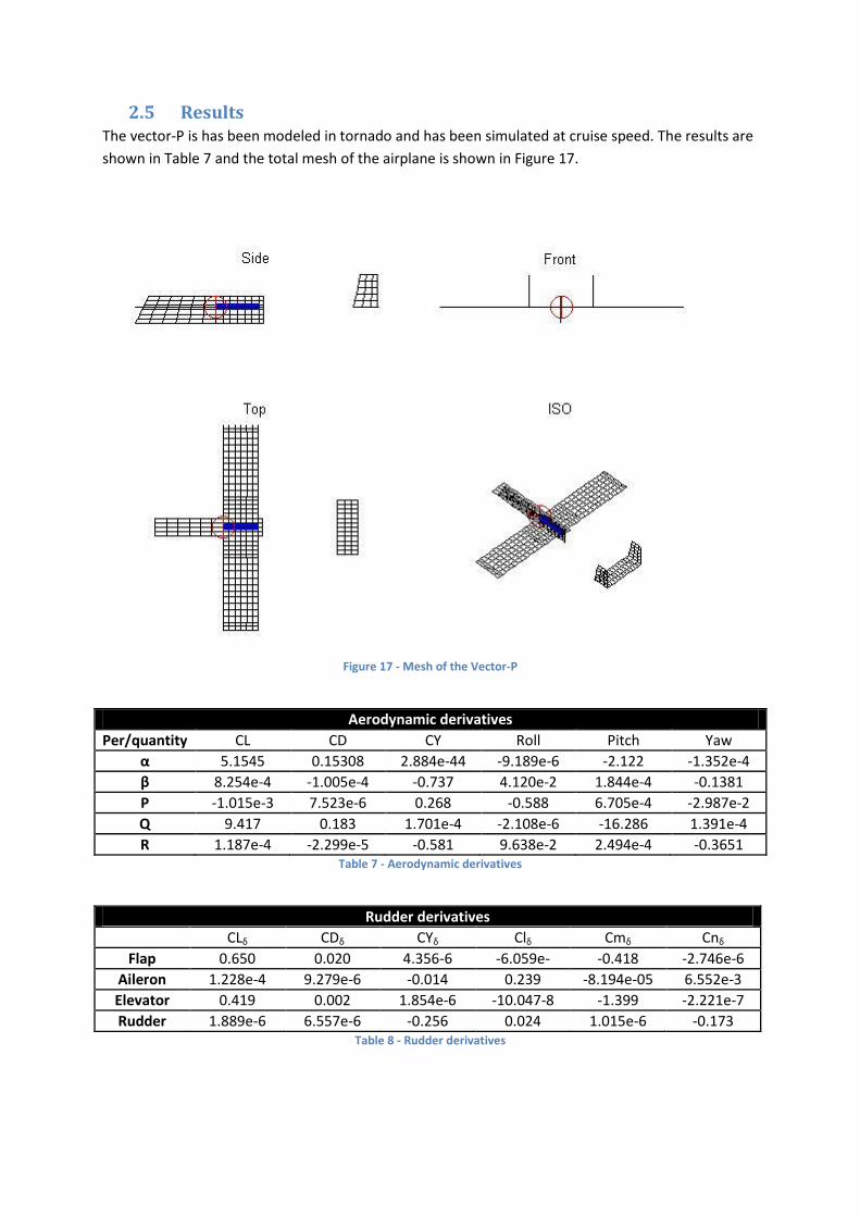
2.5 Results The vector-P is has been modeled in tornado and has been simulated at cruise speed. The results are

shown in Table 7 and the total mesh of the airplane is shown in Figure 17.

Figure 17 - Mesh of the Vector-P

Aerodynamic derivatives

Per/quantity CL CD CY Roll Pitch Yaw

α 5.1545 0.15308 2.884e-44 -9.189e-6 -2.122 -1.352e-4

β 8.254e-4 -1.005e-4 -0.737 4.120e-2 1.844e-4 -0.1381

P -1.015e-3 7.523e-6 0.268 -0.588 6.705e-4 -2.987e-2

Q 9.417 0.183 1.701e-4 -2.108e-6 -16.286 1.391e-4

R 1.187e-4 -2.299e-5 -0.581 9.638e-2 2.494e-4 -0.3651 Table 7 - Aerodynamic derivatives

Rudder derivatives

CLδ CDδ CYδ Clδ Cmδ Cnδ

Flap 0.650 0.020 4.356-6 -6.059e- -0.418 -2.746e-6

Aileron 1.228e-4 9.279e-6 -0.014 0.239 -8.194e-05 6.552e-3

Elevator 0.419 0.002 1.854e-6 -10.047-8 -1.399 -2.221e-7

Rudder 1.889e-6 6.557e-6 -0.256 0.024 1.015e-6 -0.173 Table 8 - Rudder derivatives

From Prandtl’s classical lifting-line theory there is known that Clα is equal to 2π. This lifting line theory

is like Tornado based on thin plates. Therefore it is suspected that Clα is close to that value. From

Table 7 it follows that the Clα of the Vector-P is 5.15 which is a little lower than 2π. The difference can

be explained by the fact that Prandtl’s theory, does not take the effects of the fuselage into account.

In Tornado on the other hand the effect of fuselage is taken into account and that might cause that

the Clα is a bit lower. For this reason it is assumed that the model in Tornado is a good approximation

of the real UAV.

3. CFD Calculations of the

Aerodynamic Derivatives Telemaster

The second unmanned aerial vehicle that will be modeled in Tornado is called the Telemaster. In this

chapter first the dimension of the Telemaster will be shown and some assumptions will be explained.

After that the Telemaster will be programmed in Tornado and then the number of panels will be

determined. At last the results, the aerodynamic derivatives will be shown. A picuture of the

Telemaster is shown below.

Figure 18 - Telemaster

3.1 Dimensions of the Telemaster. The Telemaster has been modeled in Solidworks by another intern, Izabele Saorin, here at ITA. From

the 3D Solidworks model, 2D drawings were made and the dimensions of the aircraft are shown. The

drawings are shown in Figure 19 and Figure 20.

Figure 19 - Dimension of the fuselage

Figure 20 - Dimensions of the wing (left), vertical tail(r) and horizontal tail (center below)

In the two figures above the dimensions of the Telemaster are given. However the dimensions are

not a hundred percent accurate. In the left picture of Figure 19 is the side view of the fuselage

shown. It can be seen that the horizontal tail and the top of the vertical tail are not parallel with each

other, but in reality this is the case. Furthermore it follows that the upper part of the back part of the

fuselage has a tapper ratio. In reality the lower part of the fuselage has a taper ration as well. This is

the reason why the top part of the vertical tail is not parallel to the horizontal tail. With the aid of

Figure 21 the dimensions are rectified for the mistakes.

Figure 21 - Adjusted shape of the back part of the fuselage

Figure 21 shows the adjusted shape of the back part of the fuselage. The dimensions of the fuselage

are calculated on the basis of the length and width of the fuselage and the fact that it is symmetric.

The dimensions are shown in Table 9.

Dimensions of the back part of the fuselage (mm)

AD AC AG GE FG BF

94 60 49 192 96 207 Table 9 - Dimensions of the back part of the fuselage

As mentioned in the chapter of modeling the Vector-P, the centre of gravity is an important

parameter. The center of gravity is not known but research about the Telemaster has pointed out

that the centre of gravity is at (0.1228 0 -0.067) with respect to the leading edge of the wing.

3.2 Modelling Telemaster To model the Telemaster in Tornado, each part, like the wing, tail and fuselage needs to be model

separately and all have different settings just like the Vector-P. In this part of the Chapter the settings

for each part of the Telemaster will be discussed separately.

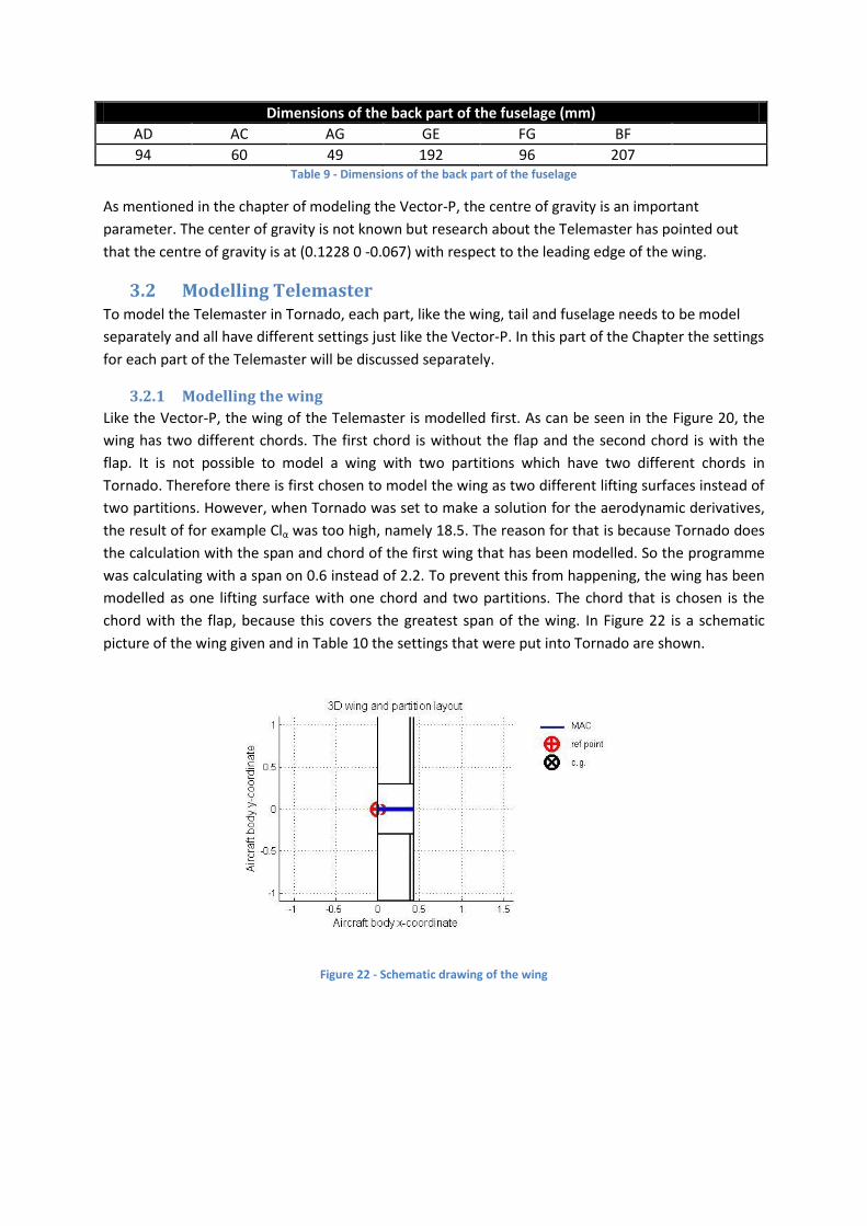
3.2.1 Modelling the wing

Like the Vector-P, the wing of the Telemaster is modelled first. As can be seen in the Figure 20, the

wing has two different chords. The first chord is without the flap and the second chord is with the

flap. It is not possible to model a wing with two partitions which have two different chords in

Tornado. Therefore there is first chosen to model the wing as two different lifting surfaces instead of

two partitions. However, when Tornado was set to make a solution for the aerodynamic derivatives,

the result of for example Clα was too high, namely 18.5. The reason for that is because Tornado does

the calculation with the span and chord of the first wing that has been modelled. So the programme

was calculating with a span on 0.6 instead of 2.2. To prevent this from happening, the wing has been

modelled as one lifting surface with one chord and two partitions. The chord that is chosen is the

chord with the flap, because this covers the greatest span of the wing. In Figure 22 is a schematic

picture of the wing given and in Table 10 the settings that were put into Tornado are shown.

Figure 22 - Schematic drawing of the wing

Settings of the wing

Partitions 1 Partitions 2

Symmetric 1 1

Apex coordinates (x,y,z) 0 0 0

Base Chord (m) 0.42929 0.42929

Half span (m) 0.3 0.8

Sweep (rad) 0 0

Dihedral (rad) 0 0

Taper 1 1

Airfoil 2412 2410

Twist (rad) 0 0

Flapped 0 1

Chord flap 0 0.0932

Flaps deflect symmetric 0 0 Table 10 - Settings of the wing

The profile of the wing was first to be estimated to be a Clark-Y profile. In Tornado the profile can

only be set by a NACA 4 digits profile. A good approximation of the Clark-Y profile is the NACA 2412.

3.2.2 Modeling the horizontal tail

As can been seen in Figure 20 the flap of the horizontal tail has a corner that is cut off. This shape can

be modeled in Tornado by calculating the taper ratio and the swept angle but it is impossible to get it

in the right orientation. In order to get it in the right orientation the taper ratio needs to be larger

than 1 which is not possible in Tornado. Therefore the flap of the tail is modeled as fully rectangular

but with the same area as the real flap. The tail and the flap will have a different chord which is not

possible to model as mentioned here above. For that reason it is chosen to model the tail as two

separate lifting surfaces. The flap of the tail will be modeled such that 97% of the lifting surfaces is

flapped. It is not possible to chosen a higher percentage because Tornado will give an error than. In

Figure 23 is the schematic view of the wing and the tail given. In Table 11 are the settings of the tail

shown.

Figure 23 - Wing and horizontal tail

Settings of the horizontal tail

Tail flap

Symmetric 1 1

Apex coordinates (x,y,z) 0.9872 0 -0.0959 1.165 0.04173 -0.0959

Base Chord (m) 0.177 0.09

Half span (m) 0.422 0.38027

Sweep (rad) 0 0

Dihedral (rad) 0 0

Taper 1 1

Airfoil 0 0

Twist (rad) 0 0

Flapped 0 1

Chord flap 0 0.97

Flaps deflect symmetric 0 1 Table 11 - Settings of the horizontal tail

3.2.3 Modeling the vertical tail

As mentioned before, the back part of the fuselage has a taper ratio in horizontal and in vertical

direction. Therefore, is the vertical tail under an angle of attack. For the model it is assumed that the

last part of the fuselage is straight so that root chord of the tail is not under an angle of attack. This

assumption is made because Tornado is unable to model the tail in the correct way.

The vertical tail has two different root chord sizes; therefore the vertical tail is also modeled as two

different lifting surfaces. For the same reason as the horizontal tail, 97% of the flap will be modeled

as a flap.

Figure 24 - Schematic view of the vertical tail

Settings of the vertical tail

Tail flap

Symmetric 0 1

Apex coordinates (x,y,z) 0.995 0 -0.064 1.165 0 -0.159

Base Chord (m) 0.17 0.223

Half span (m) 0.335 0.430

Sweep (rad) 0.2544 -0.06

Dihedral (rad) 1.57 1.57

Taper 0.3166 0.5402

Airfoil 0 0

Twist (rad) 0 0

Flapped 0 1

Chord flap 0 0.97

Flaps deflect symmetric 0 0 Table 12 - Settings of the vertical tail

3.2.4 Modeling the fuselage

The last part of the Telemaster that needs to be modeled is the fuselage. It will be modeled as two

lifting surfaces, one vertically and one horizontally, the same way as is done for the Vector-P. The

fuselage of the Telemaster has a taper ratio as well as in the vertical as in the horizontal direction.

The shape of the fuselage can exactly be modeled in Tornado by calculating the taper ratio and the

swept angle of the fuselage. If this is done the side edge of the lifting surfaces will not be parallel to

the free stream flow. This will give a numerical error because when Tornado puts panels on the lifting

surface, the side edges of the panels will not be parallel to each other. So when a horse shoe is place

on these panels, the vortex filaments will not be parallel to each which means that the sum of all

vortexes is unequal to zero and thus that the induced velocity is unequal to zero. This will cause an

inaccurate result because the vortex filaments are in reality not there so the induced velocity should

be equal to zero. Therefore the oblique edge of the lifting surface needs to be a leading edge so that

the vortex filaments of the horse shoe are parallel to each other.

The oblique side of the fuselage cannot be modeled as leading edged. Therefore is the fuselage

modeled as a number of different rectangles, which will decline in height and width in chord wise

direction. The rectangles are chosen such that the total area of the fuselage stays the same. Because

the fuselage doesn’t decline too much, it is assumed that 3 rectangles are a good approximation of

the real oblique fuselage.

There is a downside of modeling the fuselage as declining lifting surfaces. Each lifting surface will

create an extra trailing edge to the plane. This causes a tip vortex in the numerical model mean while

the tip vortexes are not present in the real situation. These lifting surfaces have a low aspect ratio

compared to the wing, which means that the strength of the vortex is relatively weak. Therefore it is

assumed that the modeled tip vortexes will have a negligible influence on the final results.

The schematic view of the fuselage is shown in Figure 25 and Figure 26 and the settings are shown in

Table 13 and Table 14.

Figure 25- Top view of the Telemaster

Figure 26 - Side view of the Telemaster

Settings of vertical fuselage

Wing 1 Wing 2 Wing 3 Wing 4 Wing 5

Symmetric 0 0 0 0 0

Apex coordinates

(x,y,z)

-0.352 0

-0.207

-0.072 0

-0.065

0.389 0

-0.193

0.692 0

-0.165

0.122 0

-0.067

Base Chord (m)

0.741 0.461 0.303 0.303 0.170

Half span (m) 0.143 0.065 0.179 0.122 0.089

Sweep (rad) 0 0 0 0 0

Dihedral (rad) 1.57 1.57 1.57 1.57 1.57

Taper 1 1 1 1 1

Airfoil 0 0 0 0 0

Twist (rad) 0 0 0 0 0

Flapped 0 0 0 0 0

Chord flap 0 0 0 0 0

Flaps deflect symmetric

0 0 0 0 0

Table 13 - Vertical fuselage

Settings of the horizontal fuselage

Wing 1 Wing 2 Wing 3 Wing 4

Symmetric 1 1 1 1

Apex coordinates (x,y,z)

-0.352 0 -0.125 0.389 0 -0.125 0.692 0 -0.125 0.995 0 -0.125

Base Chord (m) 0.741 0.303 0.303 0.1704

Half span (m) 0.07 0.057 0.045 0.020

Sweep (rad) 0 0 0 0

Dihedral (rad) 0 0 0 0

Taper 1 1 1 1

Airfoil 0 0 0 0

Twist (rad) 0 0 0 0

Flapped 0 0 0 0

Chord flap 0 0 0 0

Flaps deflect symmetric

0 0 0 0

Table 14 - Horizontal fuselage

In Table 13 and Table 14 the wings are numbered in order of the leading edge closest to the nose of

the airplane.

3.3 Number of Panels The number of panels is the only thing that needs to be determined in order to run Tornado. As

mentioned before, the number of panels is an important setting. To determine the right amount of

panels, the same procedure has been done as with the Vector-P. There has been looked at which

amount of panels Clα and Cyβ have converged to a result.

Figure 27 shows that Clα and Cyβ converges to results while the number of panels increases. Both

derivatives have converged with 616 panels.

Figure 27 - Cyβ (left) and Clα (right) against the number of panels

3.4 Results The Telemaster has been modeled in Tornado and has been simulated at cruise speed. The results

are shown in Table 15 and the total mesh of the airplane is shown in Figure 28.

Figure 28 - Mesh of the Telemaster

Aerodynamic derivatives

Per/quantity CL CD CY Roll Pitch Yaw

α 4.583 0.0758 -1.305e-3 -6.538e-6 -1.955 -5.667e-4

β 3.52e-3 -0.040 -3.9026 -1.694e-2 6.972e-3 -1.7364

P -9.839e-4 -8.658e-3 1.1424 -0.419 1.877-3 0.51328

Q 7.699 0.087 -1.608e-3 3.949e-5 -10.165 -6.702e-4

R 7.546e-4 4.49e-3 -0.815 2.15e-2 1.208e-3 -0.361 Table 15 - Aerodynamic derivatives of the Telemaster

Rudder derivatives

CLδ CDδ CYδ Clδ Cmδ Cnδ

Aileron 3.148e-4 2.074e-3 -0.4052 0.238 -4.333e-4 -0.181

Elevator 0.477 1.885e-3 7.965e-6 7.124e-7 -1.147 4.53e-6

Rudder 1.760e-4 -2.161e-4 -0.134 0.006 -3.333e-4 -0.068 Table 16 - Rudder derivatives of the Telemaster

The results of the Vector-P are assumed to be a good approximation because the Clα of the Vector-P

is a bit lower than the Clα from Prandtl’s classical lifting-line theory. The difference in the Clα is

because the Vector-P is modeled with a fuselage. The fuselage of the Telemaster is relative larger

than the fuselage of the Vector-P. This would suggest that the Clα of the Telemaster is lower than Clα

of the Vector-P. From Table 15 it follows that the Clα of the Telemaster is 4.583 which is lower than

the Clα of the Vector-P, 5.155. Therefore it is assumed that the aerodynamic derivatives of the

Telemaster are a good approximation.

.

4. Comparing Test Data with CFD

Results In this Chapter the flight experiments of the Vector-P and Telemaster will be explained and the

output of the experiments will be shown. Furthermore the equations of motion of a rigid aircraft will

be derived and applied on the data that is gotten from experiments. At last the aerodynamic

derivatives of the numeric model will be compared with the aerodynamic derivatives that are

calculated from the equations of motion.

4.1 Comparison CFD results with flight testing In this part of the chapter the aerodynamic coefficients of the Vector-P and the Telemaster, which

are calculated with Tornado, will be compared with flight test results. The flight testing of the Vector-

P has been done here at ITA but it was not possible to get good flight test data for the Telemaster.

Therefore de coefficients of the Telemaster will compared to the results of flight testing in Australia

[2]. First the general procedure to calculate the coefficients from flight testing is explained. Then the

results will be shown and the comparison will be made. To calculate the aerodynamic derivatives a

Matlab script is used. This is script is only written for the longitudinal parameters. Therefore, only the

longitudinal aerodynamic derivatives are calculated and compared.

4.1.1 Method of flight testing

To determine the aerodynamic coefficients from flight tests a method called M4V is used in both

cases. In this report there will be referred to the Vector-P. This method is called that way because it

has “four M procedures” and one “V procedure”. The four M’s stand for Maneuver, Measurement,

Methodology and Model. The V stands for validation. In Figure 29 a schematic overview of the

method is shown.

In the schematic overview of the model, the first M the Maneuver, refers input of the pilot. There are

several flight tests done in order to get data from which the aerodynamic derivatives can be

determined from. During the flight, several different maneuvers where done to determine the

Figure 29 - Scheme of determination of the aerodynamic derivatives.

Input

pilot (u)

Data acquisition (graph

with unequal time steps)

Data acquisition (graph

with equal time steps)

Compare the two graphs

of the outputs. This will

give an error Initial

parameters

Equations

of motion

Simulated

output

Cost function Algorithm to minimize

the cost function

longitudinal aerodynamic derivatives. In order to do the maneuvers, the aircraft needed some input.

The input is given by the pilot of the Vector-P. Inputs that the pilot can give are the thrust, aileron,

flaps and rudder changes. The inputs can be called the control surface deflections and can be written

in a vector:

[ ]

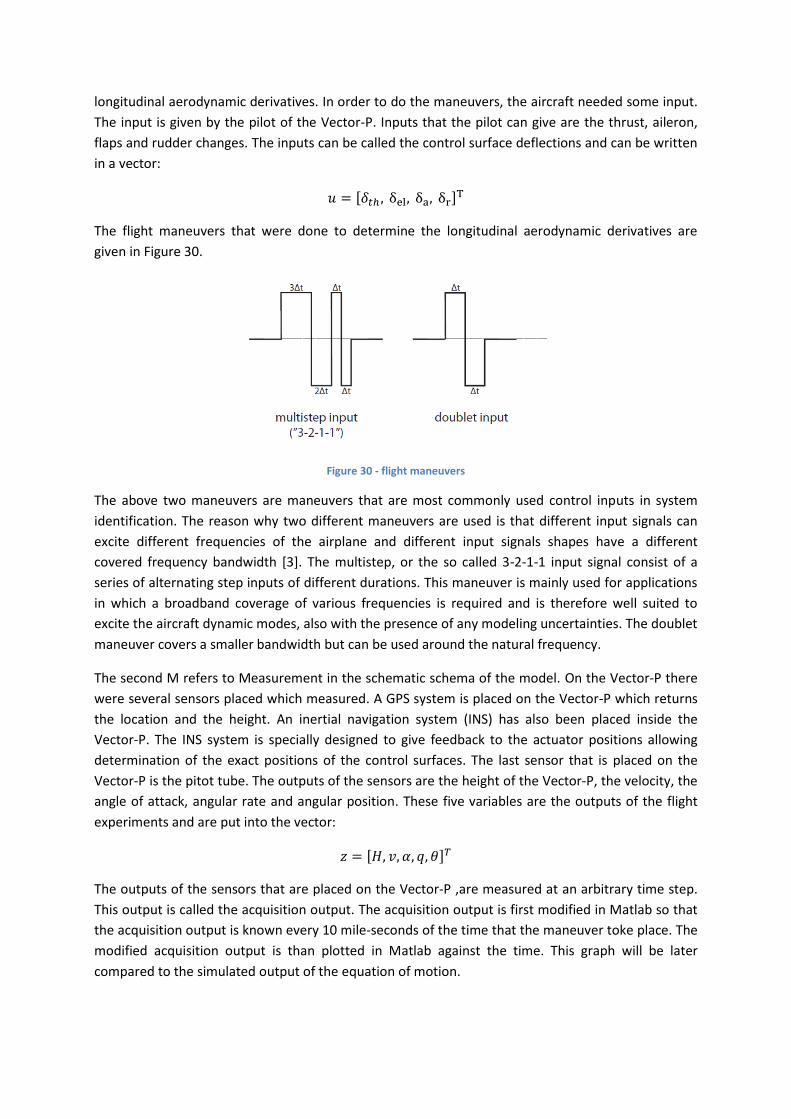
The flight maneuvers that were done to determine the longitudinal aerodynamic derivatives are

given in Figure 30.

Figure 30 - flight maneuvers

The above two maneuvers are maneuvers that are most commonly used control inputs in system

identification. The reason why two different maneuvers are used is that different input signals can

excite different frequencies of the airplane and different input signals shapes have a different

covered frequency bandwidth [3]. The multistep, or the so called 3-2-1-1 input signal consist of a

series of alternating step inputs of different durations. This maneuver is mainly used for applications

in which a broadband coverage of various frequencies is required and is therefore well suited to

excite the aircraft dynamic modes, also with the presence of any modeling uncertainties. The doublet

maneuver covers a smaller bandwidth but can be used around the natural frequency.

The second M refers to Measurement in the schematic schema of the model. On the Vector-P there

were several sensors placed which measured. A GPS system is placed on the Vector-P which returns

the location and the height. An inertial navigation system (INS) has also been placed inside the

Vector-P. The INS system is specially designed to give feedback to the actuator positions allowing

determination of the exact positions of the control surfaces. The last sensor that is placed on the

Vector-P is the pitot tube. The outputs of the sensors are the height of the Vector-P, the velocity, the

angle of attack, angular rate and angular position. These five variables are the outputs of the flight

experiments and are put into the vector:

[ ]

The outputs of the sensors that are placed on the Vector-P ,are measured at an arbitrary time step.

This output is called the acquisition output. The acquisition output is first modified in Matlab so that

the acquisition output is known every 10 mile-seconds of the time that the maneuver toke place. The

modified acquisition output is than plotted in Matlab against the time. This graph will be later

compared to the simulated output of the equation of motion.

The next step of the procedure is done with a Matlab script that is written by another student for his

master thesis at ITA in 2008 [3].

The third M of the model refers to the equations of motion. For the equations of motion there are

two different inputs. The first input in is the vector . This vector contains all the longitudinal

parameters like the initial conditions and the longitudinal aerodynamic derivatives. The parameters

are guessed and aren’t correct. The real set of parameters will be found by an iterative process. The

second input is the control surface deflections. With these inputs the equations of motion can be

solved and the output is the vector z for each time step of the maneuver. This vector z is called the

simulated output. The next step is the last M (Methodology), Matlab plots a graph of the simulated

output against the time and compares that graph with the graph of the acquisition output. This will

give an error which is the input of the cost function. The Gauss Newton Algorithm is then used to

minimize to the cost function. The minimization of the cost function will provide the solution of the

parameters θ. The whole procedure is than started again and is done until the graphs are almost

identical. An example of a graph that has converged and has not been converged yet, are shown in

Figure 31.

Figure 31 - Graph that has been converged (l) and a graph that has not been converged (r)

4.2.2.2 Results

In order to get the aerodynamic derivatives, 4 maneuvers have been done to retrieve good data. Two

of the four maneuvers are doublets maneuvers and the other two are 3-2-1-1 maneuvers. With each

of these maneuvers the procedure/identification that has been explained before has been done.

From the four identifications it follows that the result is four different vectors of θ. From the four

vector of θ, the average of each aerodynamic derivation has been calculated. The results of the

identification and the average θ are shown in Table 17.

CL0 CLα CLq CLδe CD0 Cmo Cmα Cmq Cmδe

Doublet 1

0.522 2.770 2.732 0.984 0.020 -0.081 -0.694 -13.83 -1.967 -1.134

Doublet 2

1,010 4.064 3.207 4.100 0.027 -0.114 -0.307 -17.11 -1.904 -1.018

3-2-2-1 1 0.507 3.945 3.109 0.321 0.068 -0.081 -0.443 -16.29 -6.456 -0.789

3-2-2-1 2 0.381 3.113 3.693 1.152 0.072 -0.066 -0.648 -16.42 -1.391 -1.044

Average 0.605 3.473 3.185 1.639 0.047 -0.086 -0.523 -15.91 -1.946 -0.997

Table 17 - Flight test aerodynamic derivatives

The average θ has to be validated to be sure that the longitudinal aerodynamic derivatives are

correct. For a validation another flight test maneuver is needed and the average θ is going to be the

initial set of parameters for the validation. The procedure of the identification is done with the new

initial set of parameters, the average θ. The procedure is stopped exactly after it run ones just before

Maltab calculates a new set of parameters. So no iteration has been taken place jet. The two graphs

of the acquisition output and the simulated output will be compared. This is shown in Figure 32

Figure 32 - Validation graph

In Figure 32 the acquisition output with the average θ is compared with the real output. As can be

seen from the figure, the two graphs are more or less identical, therefore there can be assumed that

average theta is a good result for the longitudinal aerodynamic derivatives of the Vector-P.

4.2 Equations of Motion To get the aerodynamic derivatives from the data from the flight experiments of the Vector-P the

equations of motion needs to be known as mentioned earlier in this report. For the derivation of the

equations of motion the following assumption are made:

The earth is flat

The earth is non-rotating

The aircraft has a constant mass

The aircraft has a rigid body

The aircraft is symmetric

There are no rotating mass like turbines

There is a constant wind

It is assumed that the aircraft body is rigid therefore the aircraft has six degrees of freedom, which

means that it has six directions it is free to follow: it can move forward, sideways, and downwards;

and it can rotate around its axes: yaw, pitch, and roll. In order to describe the state of a system that

has six degrees of freedom, six variables (unknowns) are necessary to be calculated. To solve these

six unknowns, six simultaneous equations are necessary. For an aircraft, these equations are known

as the aircraft equations of motion.

All the equations of motion of dynamic systems can be derived by using Newton’s second law. The

deferential equations can be divided into groups: the first is kinematic and the second is the flight

dynamics. To derive the aircraft equations of motion for the flight dynamics, two sets of equations

are needed to derive:

The sum of the forces on the aircraft, internal and external, are equal to its mass times its

acceleration

The sum of the moments on the aircraft, internal and external are equal to its moment of

inertia times its angular acceleration.

The derivation of the equation of motion will be started by examining the forces that act on the

aircraft.

4.2.1 Forces

Newton’s second law states that:

( )

Where the sum of all forces is that work on the aircraft (this will be explained later), is the

velocity of the center of gravity of the aircraft. The above equation is valid for the Earth-fixed

reference frame FE, where the origin 0 is at an arbitrary location on the ground. The ZE axis points

toward the ground. The XE axis is directed north and the YE axis is pointed east. To determine the

equation of motion the reference needs to be covert to an Fb reference frame. The Fb reference

frame has its origin in the center of gravity (CG) of the aircraft. The Xb axis lies in the symmetry plane

of the aircraft and points forward. The Zb axis also lies in the symmetry plane, but points downwards,

(It is perpendicular to the Xb axis.) and the YE axis is pointed east. The conversion of the reference

plane can be done with the following equation:

|

|

Substitution of this equation in the equations above gives:

|

[

]

In the equation, the following vectors are used:

[ ] [

]

Here u,v and w denote the velocity components in X, Y and Z direction. Similarly, p, q, and r denote

the rotation components around the X, Y and Z direction.

The vector contains all the forces that work on the aircraft. There are two important forces:

gravity and aerodynamic forces. The gravitational force is given by

[ ]

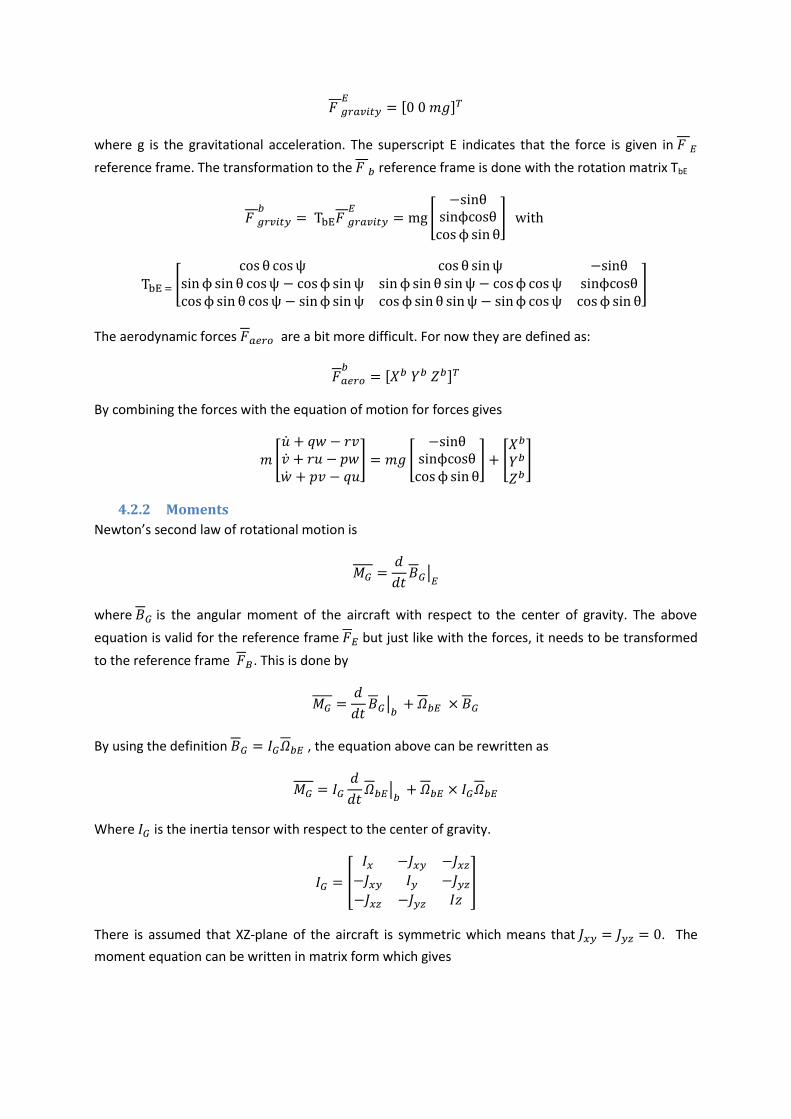
where g is the gravitational acceleration. The superscript E indicates that the force is given in

reference frame. The transformation to the reference frame is done with the rotation matrix TbE

[

]

[

]

The aerodynamic forces are a bit more difficult. For now they are defined as:

[ ]

By combining the forces with the equation of motion for forces gives

[

] [

] [

]

4.2.2 Moments

Newton’s second law of rotational motion is

|

where is the angular moment of the aircraft with respect to the center of gravity. The above

equation is valid for the reference frame but just like with the forces, it needs to be transformed

to the reference frame . This is done by

|

By using the definition , the equation above can be rewritten as

|

Where is the inertia tensor with respect to the center of gravity.

[

]

There is assumed that XZ-plane of the aircraft is symmetric which means that . The

moment equation can be written in matrix form which gives

[

( ) ( )

( ) ( )

( ) ( )

]

There are two kinds of moments that work on the aircraft. There are moments that caused by gravity

and moments caused by aerodynamic forces. The moments that are caused by gravity are zero. The

aerodynamic moments can be defined as

[ ]

This turns the moment equations into

[

( ) ( )

( ) ( )

( ) ( )

] [ ]

4.2.3 Kinematic relations

The only equations of motion that have not been found yet are the equations for the rotational

speed. These equations will follow from the kinematic relations. The rotation of the aircraft is

described by the variables . These are the variables for the FE reference system. The

rotational velocity is described by p,q and r in the Fb reference system. The relation between those is

[ ] [

] ⌈

⌉

The above equation is the rotational kinematic relation. If the equation is inverted, the equations of

motion will be

⌈

⌉ [

] [ ]

4.2.4 Longitudinal directional aircraft model

As mentioned in the previous section, only the longitudinal direction of the aircrafts is taken into

account. The longitudinal equations of motion are gotten to assume that all states and their

derivatives in lateral direction are zero. With this assumption the following longitudinal equations of

motion are found:

( )

4.3 Comparison Tornado with flight test data In this part of the chapter, the aerodynamic derivatives of the Vector-P and the Telemaster that were

determined with Tornado are compared with results of flight testing.

4.3.1 Vector-P

In the table below the corresponding longitudinal aerodynamic derivatives are shown that are

determined by Tornado and by flight testing.

CL0 CLα CLq CLδe CD0 Cmo Cmα Cmq Cmδe

Tornado 0.311 5.154 9.417 0.419 0.005 -0.146 -2.122 -16.286 -0.139

Flight testing

0.605 3.473 3.185 1.639 0.047 -0.086 -0.523 -15.919 -0.997

Table 18 - Longitudinal Aerodynamic derivatives

In Table 18 the longitudinal aerodynamic derivatives determined by the two methods of the Vector-P

are given. The first thing that can be noticed is that only one derivative of the two methods are more

or less the same, namely Cmq. The second noticeable fact is that all the signs of the aerodynamic

derivatives are the same which is positive. The rest of the aerodynamic derivatives differ a lot

between the two methods. The difference can be explained by many causes. The difference in CLα

and CD0 can be explained by the fact that the fuselage is in Tornado modeled as two flat plats. In

realty the fuselage is pretty massive and will have more influence on the flow. Therefore the CD0 in

Tornado is lower than in the flight testing and in is CLα in Tornado higher than in the flight testing.

The difference in CL0 can be explained by the fact that Tornado neglected the thickness of the wing.

Therefore the CL0 from Tornado is lower than in reality. The difference in the moment aerodynamic

derivatives and in the CLδe can be explained by the fact that the centre of gravity that is used as input

in Tornado is estimated. During the flight testing there are many thing placed inside the Vector-P like

for the sensors. Also the amount of fuel changes during the flight. These facts make it hard to

determine the center of gravity and it is very likely that the center of gravity during the flight testing

is different than what was used as an input in Tornado. The center of gravity has an important role in

de moment coefficients and on the effect of the elevator. This may explain the differences in the

coefficients.

Other reasons why there is a difference between the derivatives, is that Tornado assumed small

angles of attack. During the flight testing, the angles of attack of the maneuvers cannot be seen as

small. Furthermore is that the simulated data maybe not 100% accurate. The sensors are sensitive to

disturbance such as wind and may influence the results as well.

4.3.2 Telemaster

The aerodynamic derivatives of the Telemaster that were determined with Tornado, will be

compared with the calculated aerodynamic derivatives of Edi Sofyan [2]. Edi Sofyan determined the

aerodynamic derivative by flight testing, with the same model of the Telemaster, in Australia for his

master thesis. The aim of his master thesis was to estimate stability and control derivatives of a

remote control aircraft model from flight test data using parameter identifications techniques. For

his master he used different sensors on the aircraft than that was used for the Vector-P but the same

model was used to determine the coefficients. The corresponding aerodynamic derivatives of both

methods are shown in Table 19 and Table 20.

Derivatives Cmα Cmq

Tornado -1.955 -10.166 0.477 -1.147

Flight testing -1.283 -7.742 1.334 0.805 Table 19 - Longitudinal aerodynamic derivatives

Derivatives Tornado Flight testing

Cyβ -3.903 3.140

Cyp 1.143 -25.78

Cyr -0.815 2.794

Clβ -0.016 -0.115

Clp -0.419 0.120

Clr 0.021 -0.012

Cnβ 0.007 -2.895

Cnp 0.514 0.024

Cnr -0.361 -0.103

Cyδaileron -0.405 0.037

Cyδrudder -0.134 -0.305

Clδaileron 0.237 -0.120

Clδrudder 0.006 2.788

Cnδaileron -0.181 0.166

Cnδrudder -0.068 0.099 Table 20 - Lateral aerodynamic derivatives

In the above two tables the aerodynamic derivatives of Telemaster are given of the two different

methods. Unfortunately most of the values do not correspond. There are only a few derivatives that

are more or less the same with both methods. These derivatives are Clr , Cmα, Cmq, Cnδaileron, and

Cnδrudder From these five derivatives the signs are not always the same. The only explanation for that

could be that the definition of positive and negative of the moments is different in Tornado

compared to what was used for the flight testing. Edi mentioned in his thesis that he had problems

with the signs, which also can explain the difference.

Edi Sofyan mentioned in his conclusion of his master thesis that the sideward’s derivatives (Cyβ Cyp

Cyr ) and Clδrudder are not good estimates of the real values. This is because, according to him, he used

the wrong method to determine those four aerodynamic coefficients correctly. Therefore these

values cannot be compared with the values from Tornado.

For the other aerodynamic derivatives that don’t correspond with both methods, it is hard to explain

why they differ. One possible reason is that there were too many assumptions to model the

Telemaster in Tornado to give an accurate result. Furthermore there is not much understanding

about the theory that was used to get the aerodynamic derivatives from the flight testing. This is also

beyond the scope of this report. Therefore it is reasonable to say that is difficult to draw any

conclusion from this comparison.

4.4 The effects in the difference in the aerodynamic coefficients of

Tornado and flight tests of the Vector-P. In the previous section the aerodynamic coefficients of the Vector-P of the two methods are

compared with each other. What is not known jet is the effects of the difference in the coefficients

that has been calculated by Tornado and that have been determined by flight testing. The effect of

the difference in the aerodynamic coefficients has been simulated in Matlab.

In Matlab, the Vector-P has been programmed. This has already been done by Fabian Kluyendorf [3].

A flight maneuver is than simulated, the elevator input is shown in Figure 33

Figure 33 - Elevator input of the simulated maneuver

In Figure 33 the blue line is the input that has be programmed in Matlab. The red line is the actual

movement of the actuator of the elevator. This input has been run twice in Matlab, once with the

aerodynamic coefficients that where determine from Tornado and once with the coefficients that

were calculated with flight test. The output of the simulation is a graph of the movement of the

Vector-P with respect to the height and the velocity of the Vector-P. The results are shown below.

Figure 34 - Height during the maneuver (Tornado)

Figure 35 - Height of the Vector-P during the maneuver (Flight)

Figure 36 - Velocity of the Vector-P during the maneuver (Tornado left flight testing right)

The difference in the aerodynamic coefficients has a great effect on the maneuver of the Vector-P.

Looking had the height during the maneuver, the two graphs have an opposite shape of each other.

This is not expected, because the aerodynamic derivatives of both methods have the same sign.

Furthermore the height difference during the maneuver is with the flight aerodynamic coefficients

much larger than with the Tornado coefficients. This is more or less expected because the CLδe of the

flight testing is 4 times larger than from Tornado and the Cmδe is about 7 times higher.

From the velocity graphs of the maneuver it can be said that speed of the vector-p is much smoother

with the flight tests coefficients and the magnitude of the speed is much lower. Another noticeable

thing is that with the Tornado coefficients the Vector-P has a really small side velocity and the

velocity downwards suggests that the aircraft is losing a lot of height. This is not shown in the graph

of the height.

The main problem of the graphs is that the shape of the maneuver is not the same. New simulations

have been to done to discover what this problem causes. The aerodynamic coefficients of the flight

testing have been adjusted by 10% towards the value of Tornado. So depending on the value of

Tornado, the aerodynamic coefficients of the Vector-P of the flight tests, have been adjusted plus or

minus 10% their value. Next the maneuver is simulated in Matlab with the adjusted aerodynamic

coefficients. The coefficients have been adjusted until they are the same as Tornado or when the

results of the maneuver changes drastically.

During the adjusted of the aerodynamic coefficients, al the coefficients have reached the value of

Tornado expect Cmα meanwhile the graph of the height of the maneuver has the same shape/sign as

the graph with the coefficients of the flight tests. The value of Cmα is than further increased and the

simulation is done again. When Cmα reached the value of 1.7, the graph of the height reached its

turning point. This is shown in the figure below.

Figure 37 - The height of Vector-P during the maneuver, (Cmα = 1.7)

From these simulations it can be concluded that the Cmα that is determined with tornado is too high.

It is about four times bigger than the Cmα that was calculated from the flight tests. Apparently this

coefficient is too sensitive to allow this difference. There could be many reasons why Tornado

calculated a too big Cmα. One reason can be that the center of gravity is not placed correctly in the

model or that the center of pressure is calculated wrong by Tornado.

5. Conclusion In this report, two unmanned aerial vehicles, the Vector-P and the Telemaster, have been modeled in

Tornado to determine the aerodynamic derivatives. Tornado is a program in Matlab that uses the

Vortex lattice method to determine the derivatives. The assumptions that Tornado uses are

The flow field is incompressible, inviscid and irrotational

The lifting surfaces are thin

The angle of attack is small.

Unfortunately, Tornado is not possible t0 model the exact shapes of the unmanned aerial vehicles. It

has some limitations which will have influences on the results. The limitations of Tornado are

Only one root chord per wing

It is not possible to chosen your reference wing

The tapper ratio cannot be larger than one

The entire wing cannot be seen as a flap

The aerodynamic derivatives of the Vector-P have also been determined by flight testing. During the

flight several maneuvers have been done to retrieve good data. The maneuvers that were done are

the doublet and the 3-2-1-1 maneuver. By doing four identifications and one validation the

longitudinal aerodynamic derivatives of the Vector-P are determined. Next the results of the flight

testing are compared with the result of Tornado. Unfortunately only one derivative is more or less

the same with both methods. The difference between the other aerodynamic coefficients can be

explained by the following reasons:

Simulated data is not 100% accurate

The place centre of gravity in Tornado is different than during the flight testing

Thickness of the fuselage

The assumptions that Tornado made

The difference in the aerodynamic coefficients will have a great influence on the fly performance of

the Vector-P. In Matlab a manoeuvre was simulated with both coefficients. The two manoeuvres

were very different from each other and the velocity in both cases was not a match either. The main

reason why it was not a match is because the Cmα that was calculated by tornado is too high.

The aerodynamic derivatives of the Telemaster that were determined by Tornado have been

compared to aerodynamic derivatives that were determined by flight tests by Edi Sofyan.

Unfortunately only a few of the derivatives were a more or less the same. Most of the derivatives

were not the same. Because the flight testing and the determination of the aerodynamic coefficients

have been done by an Australian student, Edi Sofyan, it is impossible to draw a fair conclusion from

the comparison.

Appendix A Figure 38 is a schematic picture of a swept wing. In this case it can represent the vertical tail or the

first part of the vertical fuselage of the model of the Vector-P. Let’s consider it to be the vertical tail.

This figure is used to determine the swept angle.

Figure 38- A swept wing

As mentioned before the swept angle is the angle between the quarter chord line and the Y-axis, in

this case that is angle Beta. Points B and F are considered as the quarter chord point of the root

chord and the tip chord. Let’s define the origin of the local coordinates to be at point A. The length

AD is 253 mm which means that point 4 is located at x coordinate of 63.25mm. The length of EG is

180 mm which means that the x coordinate of F is 118. Now knowing this the length of BC can be

determined:

The span of the vertical tail is off course also known, namely: 340.51 mm. The angle alpha follows

from:

This means that Beta equals:

The same procedure can be done for swept part of the fuselage.

References

1. Anderson, John D, Jr.: Fundamentals of Aerodynamics, fourth edition, New York 2007

2. Sofyan, Edi: Identification of Model of Aircraft Dynamic Using Flight Testing, Royal

Melbourne Institute of Technology, Victoria, Australia 1996

3. Kluyendorf, Fabian: System Modelling and Identification of the VECTOR_P UAV, Technische

Universitat Carolo-Whilhemina zu Braunschweig