Aerial Object Detection using Learnable Bounding Boxes

Rochester Institute of Technology Rochester Institute of Technology

RIT Scholar Works RIT Scholar Works

Theses

2-2019

Aerial Object Detection using Learnable Bounding Boxes Aerial Object Detection using Learnable Bounding Boxes

Aneesh Bhat [email protected]

Follow this and additional works at: https://scholarworks.rit.edu/theses

Recommended Citation Recommended Citation Bhat, Aneesh, "Aerial Object Detection using Learnable Bounding Boxes" (2019). Thesis. Rochester Institute of Technology. Accessed from

This Thesis is brought to you for free and open access by RIT Scholar Works. It has been accepted for inclusion in Theses by an authorized administrator of RIT Scholar Works. For more information, please contact [email protected].

https://scholarworks.rit.edu/

https://scholarworks.rit.edu/theses

https://scholarworks.rit.edu/theses?utm_source=scholarworks.rit.edu%2Ftheses%2F10203&utm_medium=PDF&utm_campaign=PDFCoverPages

https://scholarworks.rit.edu/theses/10203?utm_source=scholarworks.rit.edu%2Ftheses%2F10203&utm_medium=PDF&utm_campaign=PDFCoverPages

mailto:[email protected]

Aerial Object Detection using Learnable

Bounding Boxes

by

Aneesh Bhat

February 2019

A Thesis Submitted

in Partial Fulfillment

of the Requirement for the Degree of

Master of Science

In

Computer Engineering

Aerial Object

Detection using

Learnable Bounding

Boxes Aneesh Bhat

February

2019

KATE GLEASON COLLEGE

OF ENGINEERING

A Thesis Submitted in Partial

Fulfillment

of the Requirements for the Degree of

Master of Science in

Computer Engineering

Department of Computer Engineering

i

Aerial Object Detection using Learnable

Bounding Boxes

By

Aneesh Bhat

February 2019

A Thesis Submitted in Partial Fulfillment of the Requirements for the

Degree of Master of Science

in Computer Engineering from Rochester Institute of Technology

Approved by:

Dr. Raymond Ptucha, Assistant Professor Date Thesis Advisor, Department of Computer Engineering

Dr. Clark Hochgraf, Associate Professor Date Thesis Advisor, Department of Electrical Engineering

Dr. Alexander Loui, Associate Professor Date

Committee Member, Department of Electrical Engineering

Department of Computer Engineering s

ii

Abstract

Current methods in computer vision and object detection rely heavily on neural networks

and deep learning. This active area of research is used in applications such as autonomous driving,

aerial imaging, defense and surveillance. State-of-the-art object detection methods rely on

rectangular shaped, horizontal/vertical bounding boxes drawn over an object to accurately localize

its position. Such orthogonal bounding boxes ignore object pose, resulting in reduced object

localization, and limiting downstream tasks such as object understanding and tracking. To

overcome these limitations, this research presents object detection improvements that aid tighter

and more precise detections. In particular, we modify the object detection anchor box definition to

firstly include rotations along with height and width and secondly to allow arbitrary four corner

point shapes. Further, the introduction of new anchor boxes gives the model additional freedom to

model objects which are centered about a 45-degree axis of rotation. The resulting network allows

minimum compromises in speed and reliability while providing more accurate localization. We

present results on the DOTA dataset, showing the value of the flexible object boundaries,

especially with rotated and non-rectangular objects.

iii

Contents

Signature Sheet…………………………………………………………………………………… i

Abstract…………………………………………………………………………………………... ii

Table of Contents………………………………………………………………………………... iii

List of Figures……………………………………………………………………………..……. vii

List of Tables…………………………………………………………………………………...… x

Acronyms…………………………………………………………………………………...…… xi

I Object Detection Networks

Chapter 1: Introduction………………………………………………...……………………... 1

Chapter 2: Related Work……………………………………………….…………………...… 3

Chapter 3: YOLO - You Only Look Once……………………………..…………………...… 5

3.1 Background……………………………………………………………………………….... 5

3.2 Overview of the YOLO Pipeline…………………………………………………………... 6

3.3 Non-Max Suppression……………………………………………………………...……… 9

3.4 Deficiencies of YOLO……………………………………………………………..………. 11

Chapter 4: YOLO v2- Better, Stronger, Faster………………………………………..…...… 13

4.1 Introduction………………………………………………………………………………... 13

4.2 Changes from YOLO…………………………………………………………………….... 15

Chapter 5: YOLO v3…………………………………………………………………………... 20

5.1 YOLO v3…………………………………………………………………...……………… 20

iv

5.2 Overview of YOLO v3……………………………………………………………...……... 20

5.3 Backbone Architecture……………………………...……………………………………... 23

Chapter 6: Applications of YOLO……………………..……………………………………… 29

6.1 Object Detection Networks………………………………………………………………... 29

6.2 YOLO in Aerial Imaging…..……………………………………………..………………... 30

6.3 Shortcomings of YOLO………………………………………………….………………... 31

II Methodology

Chapter 7: Oriented Bounding Boxes……………………………………….………………... 32

7.1 Experiment Methodology…………………………………......………….…………...….... 32

7.2 DOTA Dataset…......…………………………………………….….……………………... 32

7.3 Data Preprocessing………………………………………………….……………………... 34

7.4 Incorporating Angle to Annotations.…………………………....….………………….…... 36

Chapter 8: Rotating Anchor Boxes……………………………...………….…………….…... 40

8.1 Rotated Anchor Boxes………………………………....…......………….………….....…... 40

8.2 Activation of Angle…………………………………..............………….………..…...…... 40

8.3 Angle Loss.…………………………………......…………........................…………...…... 41

8.4 IOU of Boxes…………………………………......………….………….......................…... 43

8.5 Evaluating the model…………………………………..............………….…………...…... 43

Chapter 9: Rotating Anchor Boxes……………………………....………….………………... 46

9.1 Anchor Box and Wiggle Tradeoff.………………………….....………….…………...…... 46

9.2 Adding Anchor Boxes.…………………………………...........………….…………...…... 46

v

9.3 Wiggle for Anchor Boxes………………………………….......………….…………...…... 47

9.4 Training Specifications.…………………………………......…...……….…………...…... 48

Chapter 10: Rotating Anchor Boxes………………………...……….......….………………... 49

10.1 Shortcomings of Rotated Anchor Boxes.…………………….………..................…...…... 49

10.2 Selection of Anchor Box.……………………………......………….…………..........…... 49

10.3 Activation Function for Point Values.……………………......………….…………...…... 50

10.4 Calculating IOU.…………………………………......………….………............…...…... 53

10.5 Loss Function for Deformable Point Network.…………......…………....…………...…... 54

Chapter 11: Rotating Anchor Boxes………………………...………….…….......…………... 55

11.1 Motivation and Objective.……………………………......…......……….…………...…... 55

11.2 Training Scheme.…………………………………......………….…...........………...…... 55

11.3 Testing.…………………………………......………….………...........................…...…... 56

11.4 Experiments with Angle.…………………………………......………….…………...…... 57

11.5 Experiments with YOLO v3.…………………………......………….…......………...…... 57

11.6 Experiments on YOLO Rotated.…………………………......………….….………...…... 57

11.7 Experiments on YOLO Extra Anchors.…………………......………….…..………...…... 58

11.8 Experiments on Deformable YOLO.…………………………….….……….......…...…... 58

11.9 Results of Experiments.…………………………………......………….………..…...…... 58

11.10 YOLO v3.…………………………………......………….…………........................…... 60

11.11 YOLO Rotated.…………………………………......………….…………...............…... 61

11.12 YOLO – Extra Anchors.………………………………......………….…...………...…... 65

11.13 Deformable YOLO.…………………………………......………......….…………...…... 66

11.14 Time Sensitivity.…………………………………......………….…..........………...…... 68

vi

11.14 Results on Official Test Set.……………………………….…….…..........………...…... 69

Chapter 12: Rotating Anchor Boxes……………………………...…………………………... 70

12.1 Conclusions and Future Work.………………………......………….….......………...…... 70

12.2 Computer Vision in Object Detection.…………………………………...........……...…... 72

12.3 Conclusion.…………………………………......………….………….......................…... 72

References……………………………...………………………………………..……………... 76

Appendix……………………………...………………………………………………………... 79

vii

List of Figures

Fig 1.1: A typical CNN architecture for object recognition [1]..................................................... 2

Fig 3.1: The feature extractor used in [1]. The features extracted here has a dimension of 7 7

30................................................................................................................................................... 6

Fig 3.2: Output of YOLO network. Each box solves for 4 + 1 + C predictions for location,

objectness and class. Only the center cell in which the object centroid lies is responsible for

detection. ...................................................................................................................................... 8

Fig 3.3: The same object is predicted thrice in this image. This could result in false positives being

counted for this image, despite the network being partially right about object location.

[2]................................................................................................................................................ 10

Fig 3.4: An example where the score threshold is set to a lower value so that more predictions are

taken into account. [8].................................................................................................................... 10

Fig 3.5: Final output of the YOLO network on an example image.

[1].................................................................................................................................................. 11

Fig 3.6: YOLO fails to detect several cars in this image. The missed detections come from objects

that are very small or very close together. It is also unable to detect same class objects of different

sizes. [20] ...................................................................................................................................... 12

Fig 4.1: Comparison of seed and mAP scores of different object detection networks.

[3].................................................................................................................................................. 15

Fig 4.2: Object box predictions from one anchor box, belonging to one particular grid cell. [3].

The dotted lines show the anchor box while the blue box is the prediction of the network, or the

change in height and width of the anchor box. .............................................................................. 17

Fig 5.1: YOLO v3 backbone outputs. .......................................................................................... 21

Fig 5.2: The first nine convolutions of Darknet -54. The dimensions of the feature maps are shown

to the right. It is assumed that the input is a square RGB image of 832 pixels.

....................................................................................................................................................... 25

Fig 5.3: Input from the previous block fed into 8 resblocks. ....................................................... 26



viii

Fig 5.6: Input from the previous block fed into the last few convolutions to give output prediction

maps.............................................................................................................................................. 28

Fig 6.1: Visualization of object detection in a self-driving car [27]. ........................................... 29

Fig 7.1: Two crops, image 1 and image 2 of size 1024 1024 being extracted from an original

image size of 3875 5502. ............................................................................................................ 35

Fig 7.2: All possible rotations of an object. The mirror image of each of these objects would be

the same object at the same angles. ............................................................................................... 36

Fig 7.3: The object rotation starts at 10 degrees from the x axis and then increases to 45 degrees.

In the last tile, the object is rotated further along to 80 degrees, however, we calculate this to be -

10 degrees to encourage small angles of rotation. ......................................................................... 38

Fig 7.4: Such errors in annotation are approximated by the algorithm. Here the rotation of the

object is approximated to 45 degrees. In this figure, the object is drawn by the black lines and the

red lines show the annotation points that are connected by straight lines...................................... 39

Fig 8.1: Predictions for a grid cell from the YOLO – Rotated network. The values in the blue boxes

are for x, y, width and height. Alongside, we also predict angle, objectness and class.

....................................................................................................................................................... 41

Fig 8.2: Top shows a box centered at its axis. The two figures below, show its wiggle of +/- ten

degrees about its axis. ................................................................................................................... 42

Fig 8.3: The box is overlaid with its wiggle. ................................................................................. 43

Fig 8.4: Pictorial representation of intersection and union of two boxes, B1 and B2 [4].

....................................................................................................................................................... 44

Fig 8.5: Change in angle IOU factor with respect to change in angle for a wiggle of 1 degree.

....................................................................................................................................................... 45

Fig 9.1: On the left, in red are the three anchor boxes that were originally present in YOLO. To

the right, in blue are the three anchor boxes that we have added. As shown, the new anchor boxes

have the same height and width as the previous ones but are shifted by 45 degrees from their axis.

....................................................................................................................................................... 46

Fig 9.2: The six anchor boxes used by this variation of the YOLO network. The center boxes are

in red and their right and left rotations are in different shades of blue........................................... 47

Fig 10.1: The box in blue is the anchor box for which distance is measured from the corresponding

point. We have four cases as shown, where the lines in red represent distances measure from the

ix

corresponding point. The sum of all these distances are taken for each case. The case that gives

the minimum sum of distances will be selected as the optimum configuration. We use this process

to select the best anchor box as well. In this figure, the case on the top left will give the least sum

of distances.................................................................................................................................... 50

Fig 10.2: The activation function, sinh(x/3) used to predict the displacement of anchor points.

....................................................................................................................................................... 52

Fig 10.3: arcsinh(x), showing its good curve and gradient. .......................................................... 53

Fig 11.1: Detection visualization for YOLO v3, without any rotation. The pink box and circle are

detections while blue circles are ground truth. .............................................................................. 61

Fig 11.2: Detection visualization for YOLO v3, with +/- 10-degree rotation. The pink boxes are

detections while blue circles are ground truth. Note the mistaken identifications which contributed

to low scores. ................................................................................................................................ 62


detections while blue circles are ground truth. The network detects objects that are rotated by

almost +/- 25 degrees, giving false predictions. ............................................................................ 63


detections while blue circles are ground truth. The network detects large vehicles as small vehicles

which leads to lower scores............................................................................................................ 64

Fig 11.5: Detection visualization for YOLO v3 Extra Anchors. The pink boxes are detections while

blue circles are ground truth. The network accurately detects objects of all rotations.

....................................................................................................................................................... 66

Fig 11.6: Detection visualization for Deformable YOLO. The pink boxes are detections while blue

circles are ground truth. The network predictions are not restricted to rectangles or squares as can

be seen in the top right car images.................................................................................................. 67

Fig 11.7: Examples of cases where the model results were penalized based on arbitrary

rotation……………………………................................................................................................... 71

Fig 11.8: A baseball diamond that spans across almost the whole image. In this case the object

will not be detected because of its sheer size................................................................................. 71

Fig 11.9: In the left, the cars are too small to be detected. The network struggles with such

examples where the object sizes vary from a few pixels to a 20-30 pixels, as in the right............. 72

x

Fig 11.10: The cars in blue are labelled. Those in red have been missed by the annotators. Such

inconsistencies might have contributed to false detections by the network.................................. 72

Fig 12.1: A plot of height vs width of cars within the DOTA dataset. The image dimension was

1024 × 1024. We see that height ranges from 5 pixels to 80 pixels while width ranges from 2.5 to

30 pixels........................................................................................................................................ 71

xi

List of Tables

Table 3.1: Comparison of object detection methods on the Pascal VOC 2007 [5] dataset as of

2015. [1]........................................................................................................................................ 5

Table 4.1: Comparison of object detection methods on the Pascal VOC 2007 + 2012 dataset as of

2015............................................................................................................................................... 14

Table 4.2: Contributions of each of the changes to mAP scores in YOLO v2. [3]....................... 19

Table 7.1: Training method for YOLO experiments. Two sets, with initial batch sizes of 16 and

32 are trained. Training is done in two stages where, only the last two layers are trained in the first

stage and then all layers are trained in the next stage. Batch sizes, learning rates and number of

epochs were determined experimentally through trial and error. .................................................. 33

Table 11.1: Training scheme for all experiments.......................................................................... 56

Table 11.2: mAP results of 32-batch version of YOLO variants on small vehicles class of DOTA

dataset............................................................................................................................................ 59

Table 11.3: mAP results of 32-batch version of YOLO variants on small vehicles class of DOTA

dataset............................................................................................................................................ 59

Table 11.4: IOU results of YOLO variants on small vehicles class of DOTA dataset. ................ 60

Table 11.5: Time analysis for 16-batch models. ........................................................................... 68

Table 11.6: Time analysis for 32-batch models. ........................................................................... 69

Table 11.7: Results on DOTA Test Set – Top Performers. .......................................................... 70

Table 11.8: Results on DOTA Test Set – Bottom Performers. ...................................................... 70

xii

Acronyms

CNN

Convolutional Neural Network

CV

Computer Vision

FC Layer

Fully Connected Layer

FCN

Fully Convolutional Network

1

Chapter 1

Introduction

Computer vision has made great strides over the past few decades. It is now an integral part

of everyone’s lives as it is used almost everywhere, from smart phones to industrial manufacturing.

Many tasks such as autonomous driving, facial recognition and optical character recognition would

not be possible without computer vision. The high-level objective of computer vision is to extract

information from high dimensional, real world images from which to make decisions, e.g. spotting

a traffic light turn red and apply brakes to stop the car. The process of extracting such information

from an image can vary. Over the past decade, deep learning methods using convolutional filters

has emerged to be the leading technique for computer vision, aiding tasks such as image

restoration, object recognition, pose estimation and motion estimation.

Within the field of computer vision, two chief tasks dominate research; object classification

and object detection. Object classification is correctly recognizing or classifying a picture of an

object. In deep learning, this is done using a neural network with c number of outputs where c is

the number of objects the network has been trained on. Object detection is not only recognizing

the object, but also accurately localizing it within an image. As a result, object detection is

significantly more complex and is an area of intense research.

Deep learning uses Convolution Neural Networks (CNN’s) to extract information from

high dimensional images. The filters needed for such convolution operations are learned by the

network via backpropagation. Such filter values are known as parameters or weights. They may

also be accompanied by a bias or an operation that shifts the mean of the operation from origin to

some other point on a cartesian plane. A typical CNN can have anywhere from a small handful to

over a hundred convolution operations. The convolutions are usually interposed with nonlinear

activations and normalization operations. The size of filters in a CNN is called receptive field and

is important in extracting features of different frequencies from an image. A typical CNN network

for object recognition is shown in Fig 1.1.

2

Fig 1.1. A typical CNN architecture for object recognition [6].

Object detection networks typically feature more than one output. Apart from the object

class, they also calculate the position of objects within an image. This can be done as a separate

branch within the same network or as a single stream.

Research within object detection includes but is not limited to improving general detection

accuracies to improving detections for specific classes of objects, specific sized objects, improving

the speed of detection or decreasing computing power and memory footprint. This thesis focuses

on improving detection precision by giving very tight and exact location maps for objects within

an image, even with multiple classes, with minimal reduction in accuracy and speed. Several

changes are made to state-of-the-art networks to incorporate this improvement. Multiple ablation

studies are also conducted to further validate the findings. This thesis is intended to be a stepping

stone for future research in this area for the bigger goal of improving object detection and computer

vision.

3

Chapter 2

Related Work

Object detection has been the subject of much recent research due to its many applications

and uses. Datasets such as MS-COCO [7] and Pascal VOC [5] have not only fueled development

of data hungry methods but enabled fair comparison amongst methods.

One of the first deep networks to offer object detection was R-CNN [8] by Girshik et al. It

used selective search methods to first extract regions from an image and then passed each region

through an object recognition Convolution Neural Network (CNN). This was not only very slow

but was also very dependent on the selective search algorithm.

Fast RCNN [9], which made use of an ROI Pooling layer on image feature maps, gave

good object detection but still required an independent selective search algorithm.

Object detection drastically improved in speed with the introduction of a Region Proposal

Layer in Faster RCNN [10]. This was one of the first end-to-end trainable object detection network

that did not rely on an external region selection algorithm. This concept was later used in Mask

RCNN [11] along with an ROI Align layer. Mask RCNN also provided methods for not only

detecting objects but also labelling each pixel of the object with a class assignment.

Another, very important network to implement object detection, was You Only Look Once

- YOLO [1]. YOLO initially addressed speed as its primary contribution while providing

comparable detection scores. At the time it was one of the few networks to offer real time detection.

Subsequent improvements to the YOLO network included YOLO v2 [3] and YOLO v3 [12]. These

are elaborated in higher detail in the later sections of the document.

Along with YOLO, Single Shot Detector (SSD) [13] also offered excellent speed without

sacrificing detection scores. SSD discretized the output space of bounding boxes into a set of

default boxes over various aspect ratios and scales for every feature map location. It also used

predictions on different scales to detect objects of different sizes accurately.

4

Oriented Boxes

Oriented bounding box detection is a recently introduced method that allows bounding

boxes which are rotated at any angle. One of the first research methods in this area was ORN [14].

ORN uses active rotating filters which rotate while performing convolution and produce multiple

feature maps with encoded rotation information. The errors from all rotated versions are

aggregated to detect rotation of an object.

An implementation of R-CNN by Ni et el. [15] achieves state of the art detection on the

DOTA [16] dataset. The rotation was achieved by using the region proposer layer of the R-CNN

to predict bounding boxes with orientation information.

DRBoxes by Liu et al. [17] implements object detection with orientation information by

using rotated priors. This approach is perhaps the most similar method to the method introduced

in this thesis because of the usage of multiple priors. DRBoxes is based off of a VGG [18] network,

while this thesis uses the YOLO framework which is based on darknet. Further, the DRBoxes

features are extracted over only one scale. DRBoxes uses six priors, all of the same aspect ratio,

with a freedom of rotation of 15 degrees in either direction. The methods introduced in this thesis

not only use a multi-scale feature extraction network, but also explore various anchor strategies.

Results are done with different freedoms of rotation as well as on implementing rotation indirectly,

by predicting four points instead of location, dimensions and angle of the box. The introduced

methods are end-to-end trainable with real time detection.

5

Chapter 3

YOLO – You Only Look Once

3.1 Background

YOLO - You Only Look Once is a deep neural network method used for object detection.

It was introduced in 2012 by Joseph Redmon [1]. At the time of its release, it was the first real

time network that offered high quality object detection mAP scores (63.4 on Pascal VOC 2007)

[5].

Table 3.1: Comparison of object detection methods on the Pascal VOC 2007 [5] dataset as of 2015. [1]

Real Time Detectors

Detector Network Train Dataset mAP FPS

100 Hz DPM [19] 2007 16.0 100

30 Hz DPM [19] 2007 26.1 30

Fast YOLO 2007 + 2012 52.7 155

YOLO 2007 + 2012 63.4 45

Less than Real Time Detectors

Fastest DPM [20] 2007 30.4 15

Fast R-CNN [9] 2007 70 0.5

Faster R-CNN

VGG-16 [10]

2007 + 2012 73.2 7

YOLO VGG-16 [1]

[18]

2007 + 2012 66.4 21

6

It helped solved a major problem with object detection networks, which was long training

and testing times. At the time, there were several state-of-the-art object detection networks such

as Fast R-CNN and Faster R-CNN. However, they were far from real time, with frame rates being

~10 FPS. This made such networks ill-suited for real time object detection.

A part of the reason for this shortcoming with Fast R-CNN and Faster R-CNN was with

the architecture. Images had to be passed through a feature extractor. The extracted features were

then divided into regions of interest. In Fast R-CNN, the ROI selection was random while in Faster

R-CNN a region proposer network was used. The regions are then regressed over to find objects

in the image. This entire process, while being thorough takes a lot of time to train. The complexity

also means that inference time is significantly long.

YOLO eliminated such multi-stage training, reducing learnable parameters and network

complexity. By streamlining this process and reducing learnable parameters, training and inference

was made faster in YOLO.

3.2 Overview of the YOLO Pipeline

There are many similarities to YOLO and YOLO 9000. The basic YOLO pipeline is

discussed in this section. As with most object detection networks, YOLO also extracts feature

maps from an image. This is done by a standard CNN network. The specific network used for this

purpose is up to the user and can be changed as per requirement. Ideally the feature extractor must

have few learnable parameters without compromising accuracy metrics.

Fig 3.1 The feature extractor used in [1]. The features extracted here has a dimension of

7 7 30. The details of this are given below.

7

The dimensions of the feature map are dependent upon the size of the input and the close clustering

of objects in an image. A typical 244 244 3 input image will generate a 7 7 d number of

output feature maps. The number of feature maps is d as shown in (1.1):

d = B 𝑥 5 + c (1.1)

where,

B is the maximum number of objects the network will be able to predict in each cell of the 7 7

feature map.

c is the number of classes.

Fig 3.2 illustrates the output of YOLO on a 244 244 3 image.

8

Fig 3.2 Output of YOLO network. Each box solves for 4 + 1 + C predictions for location,

objectness and class. Only the center cell in which the object centroid lies is responsible

for detection.

9

In the above example a 244 244 3 images are fed into the YOLO backbone to yield a

7 7 14 feature maps. Here, B = 2 and c = 4. The network detects the presence of two objects in

the whole image, one in each grid cell. As a result, the objectness for B = 0 is predicted to be ~1

for the two particular grid cells.

The x, y locations for class dog, is predicted to be 0.5, 0.5, relative to the center of that

particular cell. For cat, it is predicted to be 0.2 and 0.5. The widths and heights for the two objects

are also predicted as per the dimensions of the objects. In Fig 1.2 the width is assumed to be w and

height h.

It should be noted that the objectness for all other grid cells will be 0. Only the center grid

cell of each object in the image is responsible for detection.

3.3 Non-Max Suppression

When the object is spread out over more than one grid cell and is large enough to cover a

greater part of the image, the network may be unable to decide the exact center of the object. As

a result, multiple grid cells may contribute to the prediction. This could result in the same object

being predicted more than once, with only slight offsets in predicted box locations. An example

is shown in Fig 3.3.

10

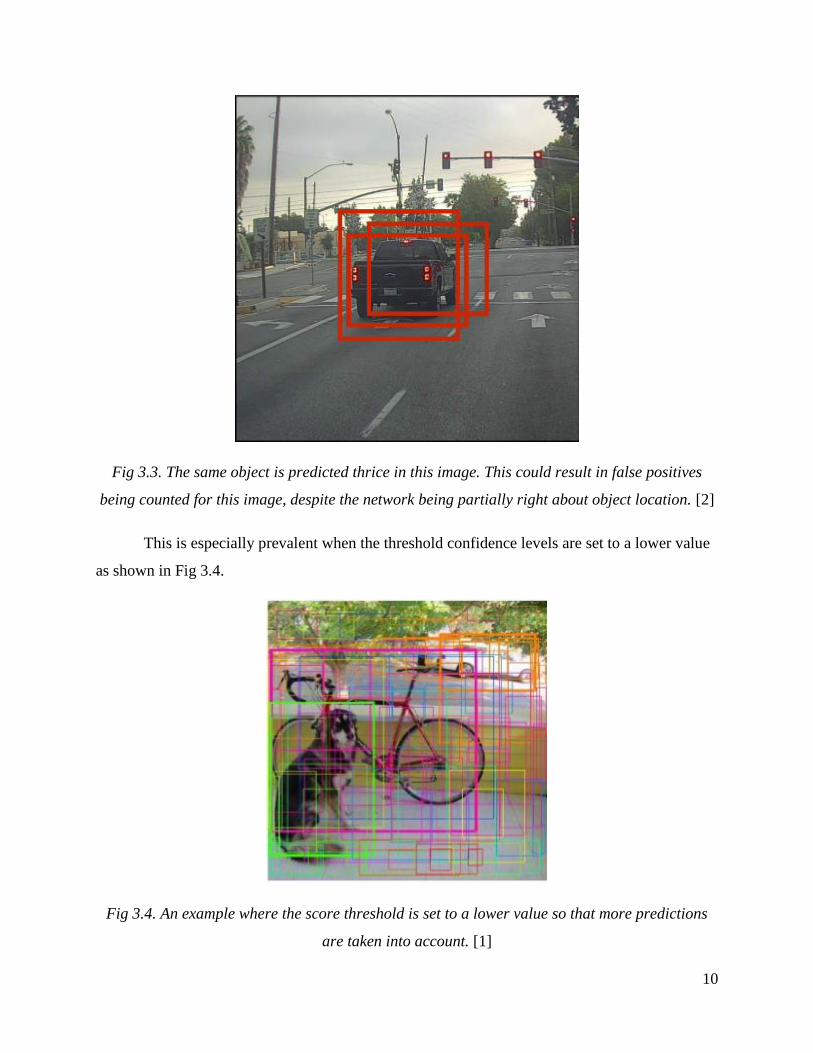
Fig 3.3. The same object is predicted thrice in this image. This could result in false positives

being counted for this image, despite the network being partially right about object location. [2]

This is especially prevalent when the threshold confidence levels are set to a lower value

as shown in Fig 3.4.

Fig 3.4. An example where the score threshold is set to a lower value so that more predictions

are taken into account. [1]

11

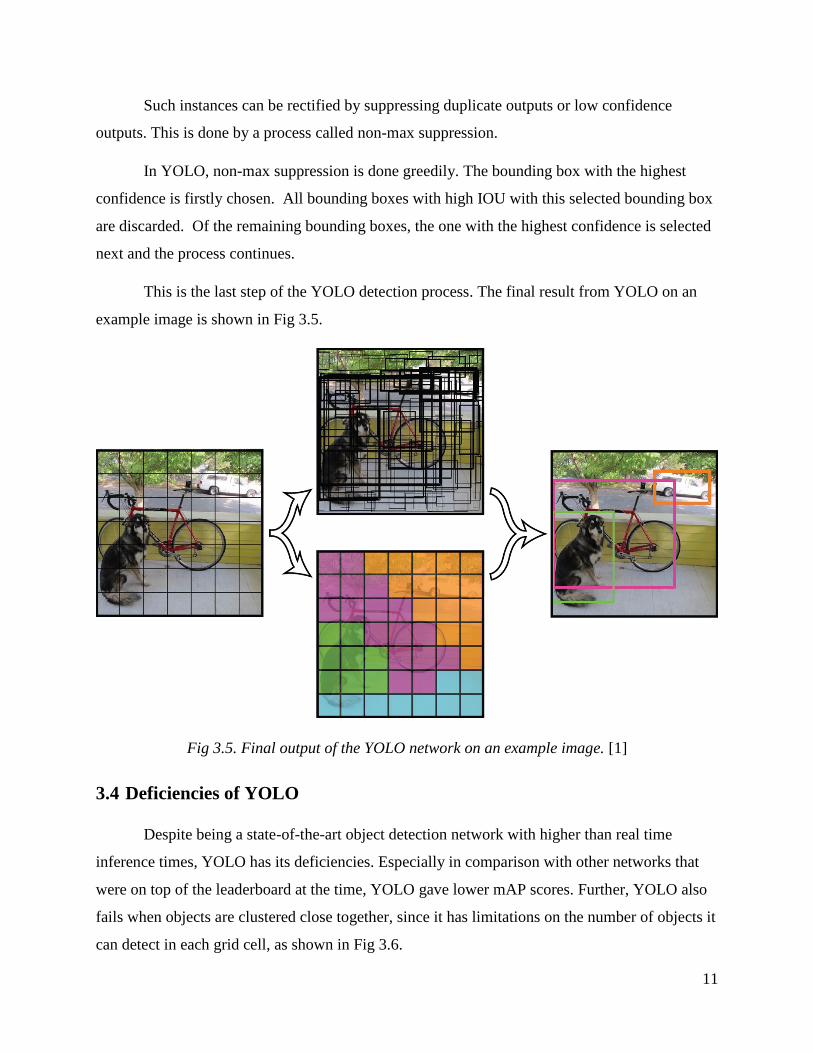
Such instances can be rectified by suppressing duplicate outputs or low confidence

outputs. This is done by a process called non-max suppression.

In YOLO, non-max suppression is done greedily. The bounding box with the highest

confidence is firstly chosen. All bounding boxes with high IOU with this selected bounding box

are discarded. Of the remaining bounding boxes, the one with the highest confidence is selected

next and the process continues.

This is the last step of the YOLO detection process. The final result from YOLO on an

example image is shown in Fig 3.5.

Fig 3.5. Final output of the YOLO network on an example image. [1]

3.4 Deficiencies of YOLO

Despite being a state-of-the-art object detection network with higher than real time

inference times, YOLO has its deficiencies. Especially in comparison with other networks that

were on top of the leaderboard at the time, YOLO gave lower mAP scores. Further, YOLO also

fails when objects are clustered close together, since it has limitations on the number of objects it

can detect in each grid cell, as shown in Fig 3.6.

12

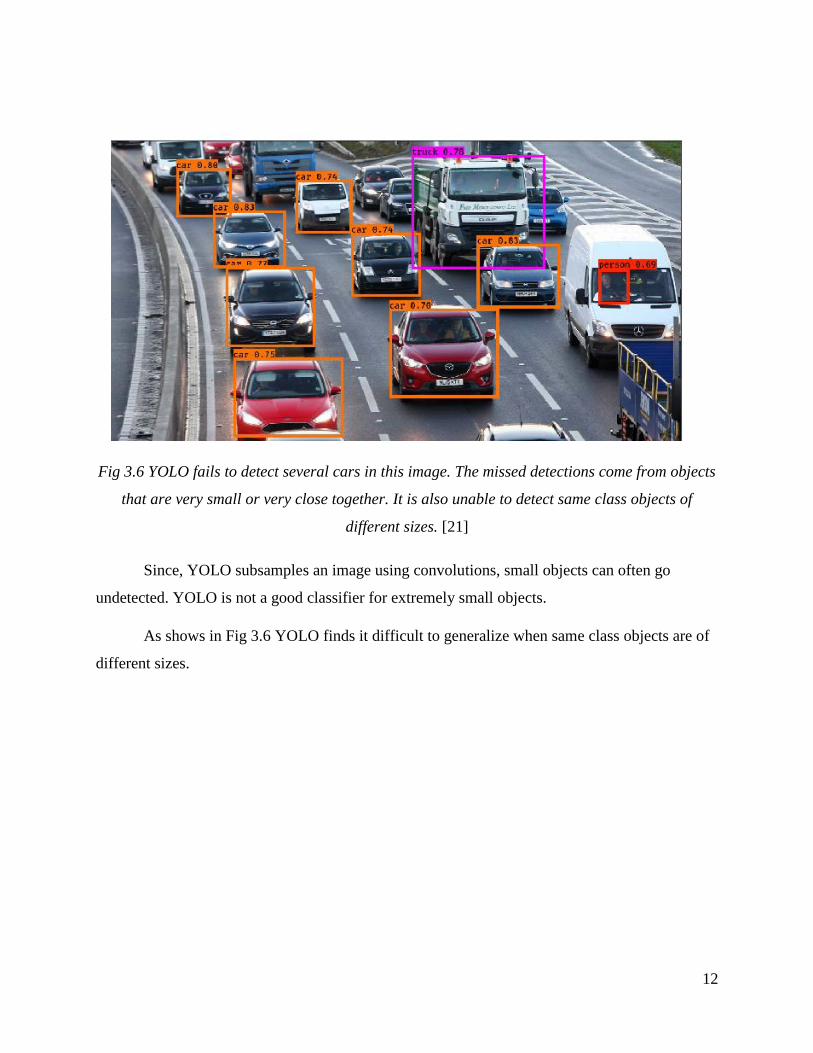
Fig 3.6 YOLO fails to detect several cars in this image. The missed detections come from objects

that are very small or very close together. It is also unable to detect same class objects of

different sizes. [21]

Since, YOLO subsamples an image using convolutions, small objects can often go

undetected. YOLO is not a good classifier for extremely small objects.

As shows in Fig 3.6 YOLO finds it difficult to generalize when same class objects are of

different sizes.

13

Chapter 4

YOLO v2 – Better, Stronger, Faster

4.1 Introduction

YOLO v2 [3] and YOLO 9000 [3] are an improvement over YOLO. It has several key

differences from YOLO. All of these networks work together to build a faster and more reliable

network. It was introduced in CVPR 2016 by Joseph Redmon and Ali Farhadi.

It was demonstrated to detect over 9000 object categories while providing real time

detection just like its predecessor. When trained on Pascal VOC, YOLO v2 provides 76.8 mAP at

67 FPS. It gives 78.6 mAP at 40 FPS, outperforming Faster RCNN with Resnet and SSD.

Apart from such advantages, it was also shown that YOLO v2 generalizes well outside of

object detection. It was shown to give good outputs for hierarchical classification giving more

detailed output on WordTree [3] representation of ImageNet [22]. This could provide benefits for

a variety of tasks.

14

Table 4.1 Comparison of object detection methods on the Pascal VOC 2007 + 2012 dataset as of 2015.

Detection Network Dataset – Pascal

Version

mAP FPS

Fast R-CNN [9] 2007 + 2012 70.0 0.5

Faster R-CNN VGG-

16 [10]

2007 + 2012 73.2 7

Faster R-CNN Resnet

[23]

2007 + 2012 76.4 5

YOLO 2007 + 2012 63.4 45

SSD300 [24] 2007 + 2012 74.3 46

SSD500 [24] 2007 + 2012 76.8 19

YOLO v2 Variations

YOLO v2 288 x 288

[3]

2007 + 2012 69.0 91

YOLO v2 352 x 352

[3]

2007 + 2012 73.7 81

YOLO v2 416 x 416

[3]

2007 + 2012 76.8 67

YOLO v2 480 x 480

[3]

2007 + 2012 77.8 59

YOLO v2 544 x 544

[3]

2007 + 2012 78.6 40

15

Fig 4.1 Comparison of seed and mAP scores of different object detection networks. [3]

4.2 Changes from YOLO

YOLO v2 incorporates several variations and changes over YOLO. All of these are listed

below and contribute to better performance. The individual contributions of each of these is given

in Table 4.2.

Anchor Boxes: The first improvement is the presence of anchor boxes. A set of user

defined anchor boxes are taken at each grid cell. The grid cell, now has the responsibility of

predicting the change in height and width of the anchor box instead of the absolute width and

height. This is seen to be more robust and in line with other state of the art object detection

networks such as Faster R-CNN. It also makes it easier for the network to learn box dimensions.

YOLO 9000 also decouples class prediction mechanism from spatial location and instead

predicts class and objectness for each anchor box.

16

In the YOLO v2 network in Table 4.1 three anchor boxes were selected for each grid cell.

If the subsamples image has 7 7 cells, there are considered to be 7 7 3 anchor boxes for that

particular feature map. Each anchor box is able to predict one object.

The equation for the prediction of width and height of an object is:

𝑏𝑤 = 𝑝𝑤𝑒𝑡𝑤 (4.1)

𝑏ℎ = 𝑝ℎ𝑒𝑡ℎ

Where,

𝑏𝑤is the width and 𝑏ℎis the height. and

𝑡𝑤 and 𝑡ℎ are network predictions for width and height respectively.

The exponential function is used because of its favorable properties during

backpropagation. Using an exponential function also prevents the prediction of negative values

since width and height cannot be negative for an object.

Anchor Box Dimensions: While anchor box dimensions are user defined, the network is

shown to benefit from picking anchor boxes that are more suited to the dataset. This is done by

using K-Means clustering to pick out nine different anchor boxes.

Constrained x, y Predictions: In YOLO, the center of an object is predicted by the

corresponding grid cell. The grid cell that falls in the center of the object is responsible for

predicting the exact x, y location of the object box, relative to itself. In region proposal networks

the coordinates are calculated as:

𝑥 = (𝑡𝑥 ∗ 𝑤𝑎) − 𝑥𝑎 (4.2)

𝑦 = (𝑡𝑦 ∗ ℎ𝑎) − 𝑦𝑎

where,

x, y are center locations of the object,

𝑤𝑎 and ℎ𝑎are the width and height of the anchor box,

17

𝑡𝑥 and 𝑡𝑦 are the predictions, and

𝑥𝑎 and 𝑦𝑎 are for the center location of the region.

By using this equation, the coordinates predicted by any one grid cell can end up in any

part of the image. YOLO v2 introduces constraints on this by allowing each grid cell to predict

coordinates anywhere within itself only. The center of an object predicted by a particular grid cell

cannot be outside of itself. The equation now becomes:

𝑏𝑥 = σ(𝑡𝑥) + 𝑐𝑥 (4.3)

𝑏𝑦 = 𝜎(𝑡𝑦) + 𝑐𝑦

Where 𝑏𝑥 and 𝑏𝑦 are the center x and y of the object.

A sigmoid operation is applied on 𝑡𝑥 and 𝑡𝑦, the predictions of the network. 𝑐𝑥 and 𝑐𝑦 is

the location of that grid cell. By this equation, the center of an object cannot extend beyond the

confines of the grid cell.

Fig 4.2 Object box predictions from one anchor box, belonging to one particular grid

cell. [3]. The dotted lines show the anchor box while the blue box is the prediction of the

network, or the change in height and width of the anchor box.

18

High resolution Classifier: YOLO was designed to take in images that were 244 244.

This made small objects very hard to recognize, especially if the image had to be resized from its

original size to 244 244. YOLO v2 is trained and tested on images that are 416 416. Further,

the backbone architecture is such that higher resolutions can be accepted by the network, though

this will increase training and inference times.

Multi Scale Training: While YOLO did not allow training or testing with images that are

of multiple scales, this is not the case with YOLO v2. Inputs can be of any dimension as long as

the number of grid cells generated is odd. This allows the training to be done on multi scale images

increasing robustness of the network. The network is allowed to generalize better and give higher

test scores that are independent of object scale.

Darknet-19: Most object detection networks use VGG [4] as their backbone. While this is

a state-of-the-art network that provides good feature extraction, there are many millions of

parameters that need to be learnt. This considerably slows down the network. YOLO v2 uses

Darkenet-19, a faster backbone. It has 19 convolution layers and 5 pooling layers. It mostly uses

3 3 convolutions and doubles the number of feature maps after each pooling step.

Training Process: The network is first trained as an object classification network. Darknet-19 is

used along with fully connected layers at the end to be trained on ImageNet 1000. Once this is

done, the last fully connected layers are removed and replaced by YOLO prediction maps. This

new network is then trained for detection. This process leverages the size of ImageNet training

data to train more generalized filters for convolution, in the first few layers.

Hierarchical Classification: YOLO v2 is trained such that ImageNet [22] labels are pulled

from WordNet [25], which is a language database that relates words to one another. For example,

in [3] “Norfolk Terrier” is classified as a type of “hunting dog” which is a type of “dog”. This

helps the network relate images and objects to one another.

The features that are extracted need to be processed to generate meaningful predictions that

correspond to object locations and classes. The next step of the YOLO pipeline focusses on

generating such predictions.

19

Table 4.2 Contributions of each of the changes to mAP scores in YOLO v2. [3]

20

Chapter 5

YOLO v3

5.1 YOLO v3

YOLO v3 was introduced by Joseph Redmon and Ali Farhadi in 2018 as an improvement

of YOLO 9000. Just like the base YOLO network, YOLO v3 also passes the image only once

through the network before making a prediction, thus retaining the “only looking once” feature of

all YOLO networks. This is one of the key features which contribute to its real time nature.

The architecture can be divided into 3 parts - the backbone, the prediction feature maps,

and the loss. This is especially advantageous, since it allows independent testing and modification

of any one module at a time.

5.2 Overview of YOLO v3

Backbone - The backbone is considered to be the feature extractor. An image is passed

through multiple convolution, pooling, batch normalization and activation layers to extract salient

features. Background information and other irrelevant features are rejected by this backbone.

Since, images can have a lot of variation between them, the backbone is typically a deep neural

network. However, the depth and number of parameters of this network must be restricted since

having complex operations at this stage can greatly slow down training and testing times of the

network. Darknet-54 is one such feature extractor that limits complexity without compromising

accuracy. The backbone network is comprised of multiple convolution operations. Since the image

is subsampled over the series of convolutions, smaller objects could lose resolution and detail. To

prevent this, outputs are taken at three different stages of convolution. These three scales of outputs

are used by the YOLO v3 network for prediction.

21

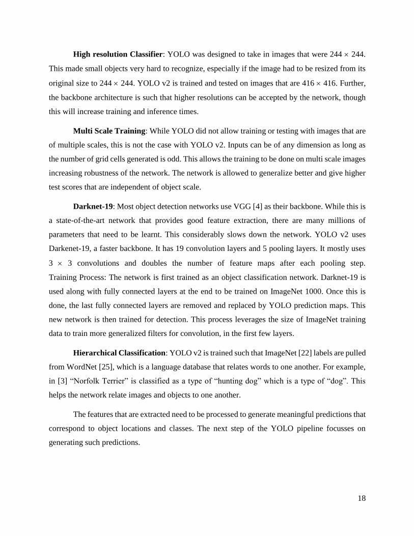
Fig 5.1 YOLO v3 backbone outputs.

Prediction feature maps - YOLO outputs set of prediction maps from an image. For

example, in Fig 5.1, each one of those outputs at the different scales is a set of B x (4 + 1 + c)

feature maps. The feature map predicts x, y locations, width, height change of anchor box along

with c outputs where c is the number of classes and B is the number of anchor boxes at one scale.

This helps to localize objects of different sizes.

YOLO v2 and YOLO v3 make use of anchor boxes for better prediction with tighter

bounding boxes.

The backbone network partitions each feature map into ss cells. Each cell for each anchor

box solves for five values: center x, y coordinates, change in w (width) and h (height) of the anchor

box and objectness or confidence of an object contained within that particular cell.

If an object spans over more than one grid cell, only the center cell is responsible for

detection of that particular object.

This prediction scheme is repeated for each of the three scales. Therefore, if there are 3

anchor boxes at each scale, the backbone predicts 3 (4 + 1 + c) feature maps for every one of the

scales.

22

However, it should be noted that as described above, each cell can only predict three objects

for each scale, or one object at any one anchor box aspect ratio for each scale. This is a notable

shortcoming of the YOLO family. This is especially of concern when there are many objects

clustered together or the objects are very small.

Losses - Because YOLO has B (5 + c) predictions at each of the ss cells, it has to have

losses for all the different types of predictions. The localization loss function measures errors in

the location and size of the predicted bounding box. Therefore, it is responsible for prediction of

x, y locations of the object center as well as w and h of the object:

λ𝑐𝑜𝑜𝑟𝑑𝛴𝑖=0𝑠2

𝛴𝑗=0𝐵 𝜑[(𝑥𝑖 − �̂�𝑖)2 + (𝑦𝑖 − �̂�𝑖)2] +


𝛴𝑗=0𝐵 𝜑 [√𝑤𝑖 − √�̂�𝑖)2 + (√ℎ𝑖 − √ℎ̂𝑖)

2

] (5.1)

Where,

λcoord increase in weight for the loss in boundary box coordinates.

Φ = 1 if the jth boundary box in cell i is responsible for detecting object, otherwise 0

λcoord is a factor that gives unequal weightage to the losses of objects based on their

bounding box sizes. Smaller objects will have higher loss factor, while bigger ones have lower

loss factor.

Confidence loss is expected to allow the network to detect the presence of an object. It is a

measure of objectiveness. If an object is detected in the one of the ss cells, the loss for that

particular cell is

𝛴𝑖=0𝑠2

𝛴𝑗=0𝐵 𝜑(𝐶𝑖 − �̂�𝑖) (5.2)

Where,

Ĉi is the box confidence score of the box j in cell i.

23

If an object is not detected, the loss becomes


𝛴𝑗=0𝐵 𝜑(𝐶𝑖 − �̂�𝑖) (5.3)

Finally, at each cell we need to determine the likelihood of each of the c classes. The

class loss is analogous to a cross-entropy loss for a classification network.

𝛴𝑖=0𝑠2

Σ𝑐∊𝑐𝑙𝑎𝑠𝑠𝑒𝑠𝜑(𝑝𝑖(𝑐) − �̂�𝑖(𝑐))2 (5.4)

The total YOLO loss can be described as


𝛴𝑗=0𝐵 𝜑[(𝑥𝑖 − �̂�𝑖)2 + (𝑦𝑖 − �̂�𝑖)2] +


𝛴𝑗=0𝐵 𝜑 [√𝑤𝑖 − √�̂�𝑖)2 + (√ℎ𝑖 − √ℎ̂𝑖)

2

] +

𝛴𝑖=0𝑠2

𝛴𝑗=0𝐵 𝜑(𝐶𝑖 − �̂�𝑖) + λ𝑐𝑜𝑜𝑟𝑑𝛴𝑖=0

𝑠2𝛴𝑗=0

𝐵 𝜑(𝐶𝑖 − �̂�𝑖) +

𝛴𝑖=0𝑠2

Σ𝑐∊𝑐𝑙𝑎𝑠𝑠𝑒𝑠𝜑(𝑝𝑖(𝑐) − �̂�𝑖(𝑐))2 (5.5)

5.3 Backbone Architecture

Darknet-54 has 54 convolution layers that resize an image from W H to prediction maps

of three different scales. This section will review this architecture. Fig 2.4 shows an image being

fed into the network. The image goes through multiple convolutions, each using leaky ReLU and

batch normalization. It should be noted that there are skip connections between layers to prevent

vanishing gradients. Skip connections are implemented between layers by a simple addition

operation. The result of this is that none of the three dimensions change, only the value at each

pixel changes.

24

It should be noted that rather than pooling, the image is resized using convolution

operations with a stride of 2. In this particular block, the image is resized from W H to W/4

H/4. An 832 832 3 image will be resized to 208 208 128. Henceforth, two convolutional

layers with a skip layer input from a preceding layer shall be referred to as a resblock . For example,

the figure below has one residual layer with 64 filters and two residual layers of 128 filters.

25

Fig 5.2. The first nine convolutions of Darknet -54. The dimensions of the feature maps

are shown to the right. It is assumed that the input is a square RGB image of 832 pixels.

26

The output of the block in Fig 5.2 is fed to the block shown in Fig 3.3.

Fig 5.3 Input from the previous block fed into 8 resblocks.

The output from this block is taken to the last few layers. This output shall be called scale

2. The input of this block would be 208 208 128 and the output would be 104 104 256.


27

This layer too serves as an important part of the last few layers. The output which would

be 52 52 512 in our previous example shall be called scale 1.


By our example, the output should now be 26 26 1024.

28

Fig 5.6 Input from the previous block fed into the last few convolutions to give output

prediction maps.

The prediction maps from the above layers are fed into the loss function. If in testing state,

the feature maps undergo non-max suppression to give outputs with the location of objects.

29

Chapter 6

Applications of YOLO

6.1 Object Detection Networks

Object detection has been a major area within computer vision research- improving mAP

scores, detection times and reliability of object detection networks. As a result, several applications

have been improved by incorporating computer vision.

6.1.1 Autonomous Cars

Autonomous driving is one of the most important technologies that has benefited directly

because of improvement in object detection and computer vision. Several car manufacturers have

already integrated some level of autonomy in their production cars. For example, Tesla cars have

already incorporated lane keeping, driving assist and collision detection [26]. Waymo has also

contributed greatly to this area by deploying self-driving cars for taxi’s in Phoenix, Arizona [27].

Fig 6.1 Visualization of object detection in a self-driving car [28].

30

Several car companies have declared that they will have full autonomy by 2025 [29] [30],

allowing cars to drive themselves without any user input. Such developments have only been

possible because of the major strides in object detection networks. Deep learning is allowing cars

to comprehend roads better, and recognize objects such as cars, trucks and pedestrians.

6.1.2 Retail

Several retailers have already made use of object detection in varying capacities. Amazon

Go uses object detection to automatically charge customers for products and eliminate long

checkout lines. This has been deployed at limited capacity at Seattle [31]. By detecting products

and automatically noticing their presence or absence, retailers can use object detection networks

to detect item theft and stock inventory.

6.1.3 Aerial Imaging

There are several applications within aerial imaging that can be simplified using object

detection. In security and surveillance, detection of vehicles and humans can be used to aid law

enforcement and improve tracking of objects of interest. Many companies have also invested in

deep learning to assist agriculture and resource detection. Ceres Imaging is one such company that

uses aerial imaging to detect agricultural yield and resource management. Improvements in high

resolution satellite imagery and drone imaging have introduced new avenues to explore.

6.2 YOLO in Aerial Imaging

YOLO is an excellent network that is well suited for aerial object detection. This is partly

because of the real time nature which allows fast moving objects to be easily detected and tracked.

This is especially useful in applications such as missile technology and police surveillance of

suspects.

The lightweight nature of the networks contributes to its suitability for drone imagery.

Lightweight drones can benefit from using minimum hardware to suit aerial object tracking

applications. This allows them to get away with using CPU’s for running YOLO instead of a heavy

GPU. Weight and space are also saved by reducing power requirements.

31

6.3 Shortcomings of YOLO

All three version of YOLO address one of the most important issues with deep learning for

object detection- timing. YOLO is an excellent network for applications that demand real time

detection such as aerial imagery.

However, there are several shortcomings of YOLO that need to be addressed. These

shortcomings prevent or hinder several applications within aerial imaging and need more research.

1. Tightness of boxes – Despite being an excellent network in terms of speed and detection

accuracy, YOLO does not give box detection that are as accurate or tight as several other

state of the art networks such as Mask R-CNN [11] or Faster R-CNN [10]. This could be

problematic when objects are close together and tracking is necessary.

2. Overlapping objects – Because of the YOLO architectures, they are limited in how many

objects they can detect within one grid cell. Depending on how the network is designed,

YOLO v3 can detect up to B S objects in each grid cell where B is the number of anchors

in each cell and S is the number of scales.

3. Orientation of boxes – Several networks such as Mask R-CNN and Fully Convolutional

Networks [32] offer semantic segmentation. This not only provides tight bounding boxes

but can also be used to draw oriented boxes around objects. This can be used to gain other

information, such as trajectory of a moving object and placement.

32

Chapter 7

Oriented Bounding Boxes

Native YOLO v3 falls short in providing tightness of bounding boxes when objects are

placed orthogonally. This is detrimental to computer vision. In this thesis, we explore ways in

which YOLO v3 can be modified to provide better bounding boxes for objects without

compromising on mAP scores. We explore several methods to provide such oriented bounding

boxes and compare them to each other, laying a baseline for future research. To verify results and

visualize them, experiments are conducted on the DOTA dataset [15].

7.1 Experiment Methodology

Changes to YOLO v3 are done in stages in order of simplicity. The entire process can be

divided into three subprocesses:

1. Allowing anchor boxes to rotate.

2. Adding extra anchor boxes while restricting rotation.

3. Changing YOLO v3 to predict four points instead of center, height and width.

All experiments are carried out using Keras with Tensorflow back-end. The methodology

for each of the subprocesses mentioned above are specified in higher detail in the next few

chapters. Each of the resulting networks are trained and tested on the DOTA large scale aerial

dataset.

All networks use YOLO v3 weights that are pretrained on the MSCOCO dataset [7]. Two

sets of experiments with two different batch sizes are conducted. Details about the training

methods are given in Table 7.1.

33

Table 7.1 Training method for YOLO experiments. Two sets, with initial batch sizes of 16

and 32 are trained. Training is done in two stages where, only the last two layers are trained in

the first stage and then all layers are trained in the next stage. Batch sizes, learning rates and

number of epochs were determined experimentally through trial and error.

Stage 1

Set 1 Set 2

Trainable Layers 249 – 251 in 251 249 – 251 in 251

Batch Size 32 16

Epochs 25 25

Learning Rate (with

decay)

0.01 0.01

Stage 2

Trainable Layers 251/251 251/251

Batch Size 4 4

Epochs 10 10

Learning Rate (with

decay)

0.001 0.001

7.2 DOTA Dataset

DOTA [15] is a large-scale aerial imaging dataset that was captured by satellites. It consists

of 1411 images of various resolutions and aspect ratios. The aspect ratios vary from 1024 1024

to as extreme as 500 3000. The dataset consists of 15 labelled classes consisting of {plane,

baseball-diamond, bridge, ground-track-field, small-vehicle, large-vehicle, ship, tennis-court,

basketball-court, storage-tank, soccer-ball-field, roundabout, harbor, swimming-pool, helicopter}.

Each object is annotated with each of the four corner points, class label and difficulty. The points

are labelled in clockwise order starting from the front left point of the object. The size of the objects

themselves vary within a class and also between classes. For example, a small vehicle can be

anywhere from three to five pixels to twenty-twenty five pixels. At the same time a roundabout

can be around 500 pixels. There can be as many as 500 objects in an image, in different classes.

34

7.3 Dataset Preprocessing

Since YOLO is agnostic to image size, the architecture itself does not oppose the wide

variations in aspect ratio or image size. However, using such images reduces the relative size of

objects within the image, making it harder for the network to learn. Hence, the images are cropped

to 1024 1024 chunks from large and unbalanced sizes of ~ 3000 1000. This is done by using a

sliding window approach recommended by [15]. Cropping ensures that the images are all of equal

sizes and aspect ratio. The number of images is also expanded to 30628.

Using an image size of 1024 1024 would put extremely high strain on the GPU used to

train YOLO v3 and its variants. Such an experiment would need compromises on batch size, which

could lead to a very noisy loss curve. Hence, the images are further resized to 832 832. This was

seen to be a good compromise between batch size and image size.

35

Fig 7.1 Two crops, image 1 and image 2 of size 1024 1024 being extracted from an

original image size of 3875 5502.

36

7.4 Incorporating Angle to Annotations

Be default the dataset does not include angle. We calculate angle at the time of preparing

the dataset, to be fed into the network.

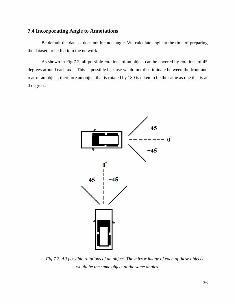
As shown in Fig 7.2, all possible rotations of an object can be covered by rotations of 45

degrees around each axis. This is possible because we do not discriminate between the front and

rear of an object, therefore an object that is rotated by 180 is taken to be the same as one that is at

0 degrees.

Fig 7.2. All possible rotations of an object. The mirror image of each of these objects

would be the same object at the same angles.

37

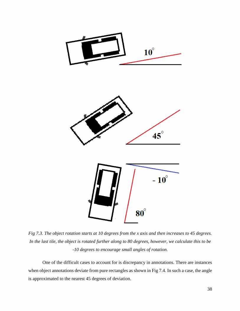
To calculate the angle of rotation of each object, we measure the angles of inclination of

two adjacent sides of the object. We always measure the angle of inclination of an object from the

x-axis. Since the objects are rectangular, one of the angles of inclination must be less than or equal

to 45 degrees. This is shown in Fig 7.3 where the object orientation increases from 0 degrees to 45

degrees. In the last tile, the object inclination increases further to 80 degrees, however by the

algorithm, we take this inclination to be –10 degrees instead. This is to reduce the amount of

rotation required to be predicted by the network. We try to keep the degree of rotation as small as

possible to put less strain on the learning process of the network.

We find this method to be efficient and reliable in most cases. By using this method both

training and testing of the network is simplified. Visualization is also more intuitive and better

written using this method.

We also find that the number of edge cases when using this method is minimal and is

discussed later. Further, the edge cases are eliminated when using deformable boxes which we will

elaborate on in the coming chapters.

38

Fig 7.3. The object rotation starts at 10 degrees from the x axis and then increases to 45 degrees.

In the last tile, the object is rotated further along to 80 degrees, however, we calculate this to be

-10 degrees to encourage small angles of rotation.

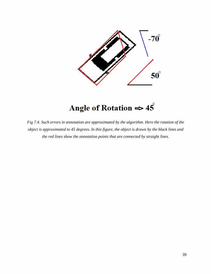
One of the difficult cases to account for is discrepancy in annotations. There are instances

when object annotations deviate from pure rectangles as shown in Fig 7.4. In such a case, the angle

is approximated to the nearest 45 degrees of deviation.

39

Fig 7.4. Such errors in annotation are approximated by the algorithm. Here the rotation of the

object is approximated to 45 degrees. In this figure, the object is drawn by the black lines and

the red lines show the annotation points that are connected by straight lines.

40

Chapter 8

Rotating Anchor Boxes

8.1 Introducing Rotation

While there have been papers that have implemented rotated predictions for objects, none

of them have incorporated these rotations for YOLO v3 or any other real time network. The first

method of implementing rotation is to allow the rotation of the anchor boxes themselves. In YOLO

v3 and YOLO v2, the anchor boxes had the freedom to morph their height and width to suit the

object being predicted. Similarly, we introduce the ability to morph angle as well.

8.2 Rotated Anchor Boxes

YOLO v3 uses anchor boxes in each grid cell to accurately predict the size of objects. The

number of predictions at each grid cell, for each scale becomes anchors (5 + C). This is just

enough to predict the objectness, x, y location, height and width of the object, along with C class

labels. This is acceptable for cases when the object is guaranteed to be vertical or horizontal,

however, it fails with rotated objects. As a starting point, we include the angle of rotation of the

box as an addition parameter for YOLO v3 to predict. Including the angle, the number of

predictions becomes anchors (5 + 1 + C). This is shown in Fig. 8.1 where the network processes

the picture and output predictions for x, y, width, height, angle, objectness and angle.

41

Fig 8.1 Predictions for a grid cell from the YOLO – Rotated network. The values in the blue

boxes are for x, y, width and height. Alongside, we also predict angle, objectness and class.

8.3 Activation of Angle

A sigmoid was used for the activation of x, y coordinates and an exponential function was

used for width and height. The activation function for angle must be differentiable, linear in the

range of freedom of movement in degrees and preferably predefined in Keras. One of the steps

taken in the process is to visualize the box as being centered at 0 degrees and then allowed to

‘wiggle’ a certain amount clockwise and counterclockwise. The total wiggle area is its freedom of

movement. The angle activation function used is

Ө = 𝑤𝑖𝑔𝑔𝑙𝑒 𝑥 (𝜎(𝑝𝑟𝑒𝑑) −1

2) (8.1)

The output of the network is run through a sigmoid activation to scale it from 0 to 1. It is

shifted by half, to change the scaling to -0.5 to 0.5. To visualize the allowable bounding box, the

total wiggle amount in degrees is multiplied so that the wiggle of the box becomes − 𝑤𝑖𝑔𝑔𝑙𝑒

2 to

42

𝑤𝑖𝑔𝑔𝑙𝑒

2 degrees. This is shown in Fig 8.2 and 8.3 where all anchor boxes for a scale are centered

around their axes but have the freedom to wiggle a certain amount around zero.

Fig 8.2 Top shows a box centered at its axis. The two figures below, show its wiggle of +/- ten

degrees about its axis.

43

Fig 8.3 The box is overlaid with its wiggle.

8.4 Angle Loss

We experimented with two different types of losses for angle, cross entropy as well as

square loss. In both cases, the angle was scaled from 0 to 1. For example, if a box was given the

freedom to rotate between -10 degrees to 10 degrees, it would be scaled from 0 to 1 before feeding

to the loss function.

For cross entropy loss, we divided the angle levels from 0 to 1 into 10 buckets. It was

expected that this would be easier to learn with a tradeoff in accuracy of angle.

Square loss was simply a square of the difference between scaled values of prediction and

ground truth as shown in equation below.

𝐴𝑛𝑔𝑙𝑒 𝑙𝑜𝑠𝑠 = (𝑃𝑟𝑒𝑑𝑖𝑐𝑡𝑒𝑑 𝐴𝑛𝑔𝑙𝑒 − 𝐺𝑟𝑜𝑢𝑛𝑑 𝑇𝑟𝑢𝑡ℎ 𝐴𝑛𝑔𝑙𝑒)2 (8.2)

8.5 IOU of Boxes

Adding an angle parameter to a bounding box, introduces additional complexity for

calculating IOU. Without angle, the IOU is calculated by (8.3) and shown in Fig. 8.4.

𝐼𝑂𝑈 =𝐴𝑟(𝐼𝑛𝑡𝑒𝑟𝑠𝑒𝑐𝑡𝑖𝑜𝑛)

𝐴𝑟(𝑝𝑟𝑒𝑑𝑖𝑐𝑡𝑒𝑑 𝑏𝑜𝑥)+𝐴𝑟(𝐺𝑟𝑜𝑢𝑛𝑑 𝑡𝑟𝑢𝑡ℎ 𝑏𝑜𝑥) (8.3)

44

Fig 8.4 Pictorial representation of intersection and union of two boxes, B1 and B2 [4].

By including angle, we can no longer use this method of calculating IOU. We calculate the

new IOU by first treating it as if it were not rotated at all. We first use (8.2) to calculate its IOU,

then we multiply this by an angle IOU factor, that is defines in (8.3).

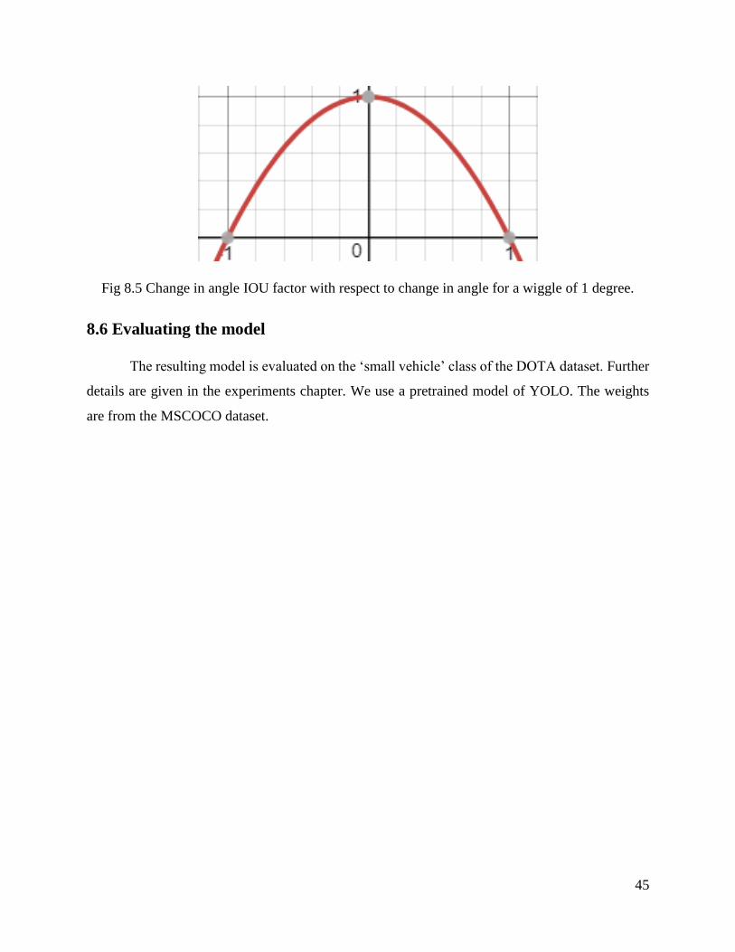
𝑎𝑛𝑔𝑙𝑒 𝐼𝑂𝑈 𝑓𝑎𝑐𝑡𝑜𝑟 = 1 − (Ө𝑝𝑟𝑒𝑑𝑖𝑐𝑡𝑒𝑑− Ө𝐺𝑟𝑜𝑢𝑛𝑑 𝑇𝑟𝑢𝑡ℎ)

𝑤𝑖𝑔𝑔𝑙𝑒

2

(8.4)

This ensure that the IOU curve, with respect to difference in angle changes as shown in Fig

8.5.

45

Fig 8.5 Change in angle IOU factor with respect to change in angle for a wiggle of 1 degree.

8.6 Evaluating the model

The resulting model is evaluated on the ‘small vehicle’ class of the DOTA dataset. Further

details are given in the experiments chapter. We use a pretrained model of YOLO. The weights

are from the MSCOCO dataset.

46

Chapter 9

Rotations with Extra Anchor Boxes

9.1 Anchor Box and Wiggle Tradeoff

While increasing wiggle for anchor boxes will allow them to accommodate greater

variations of objects, it can come at a price. Increasing this wiggle means that there will be a greater

range of angles for it to learn. Further, the greater the wiggle, the increased difficulty in predicting

the ground truth angle. For these reasons, it is worth exploring the idea of adding more anchor

boxes, centered at various angles, while reducing wiggle in each of the boxes.

We set up a baseline for adding anchor boxes and experiment with changes in IOU and

mAP scores for the same dataset.

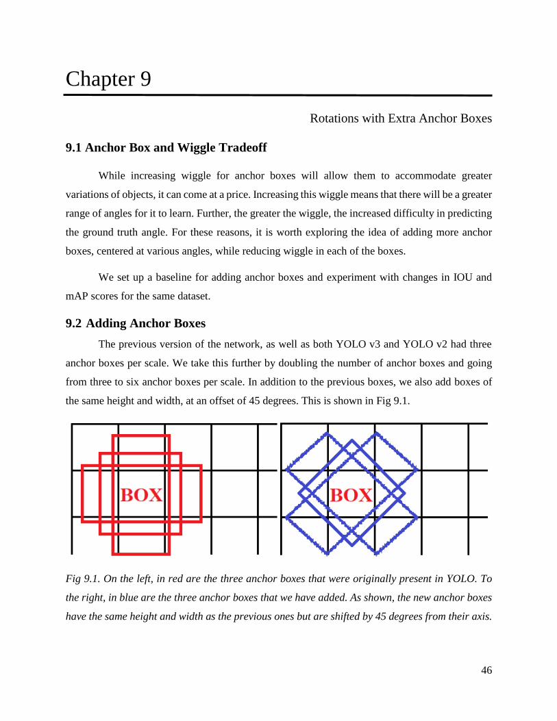
9.2 Adding Anchor Boxes

The previous version of the network, as well as both YOLO v3 and YOLO v2 had three

anchor boxes per scale. We take this further by doubling the number of anchor boxes and going

from three to six anchor boxes per scale. In addition to the previous boxes, we also add boxes of

the same height and width, at an offset of 45 degrees. This is shown in Fig 9.1.

Fig 9.1. On the left, in red are the three anchor boxes that were originally present in YOLO. To

the right, in blue are the three anchor boxes that we have added. As shown, the new anchor boxes

have the same height and width as the previous ones but are shifted by 45 degrees from their axis.

47

9.3 Wiggle for Anchor Boxes

Since, we have more anchor boxes covering each grid cell, we can restrict the wiggles of

each anchor box to 45 degrees, or 22.5 degrees to either side of their center. This is the minimum

wiggle angle at which objects at all rotations can be covered. Increasing the wiggle beyond this,

will only cause the boxes to predict identical ground truth objects, giving us no added advantage.

At the same time, reducing the wiggle prevents objects at higher rotation angles from being

detected. Fig 9.2 shows the six anchor boxes along with their freedom of rotation about their axes.

Fig 9.2. The six anchor boxes used by this variation of the YOLO network. The center boxes are

in red and their right and left rotations are in different shades of blue.

48

9.4 Training Specifications

All other parameters, losses and IOU metrics remain unchanged from the previous

network. We have designed this experiment so that any changes in results are only because of the

added anchors and not due to any other reason. This makes all tests reproducible and also makes

it easier to gauge the effect of each change on accuracy metrics. The results of the experiment as

well as the hyperparameters are presented in the results section.

49

Chapter 10

Deformable Anchor Boxes

10.1 Shortcomings of Rotated Anchor Boxes

While rotated anchor boxes are a simple solution to an important problem, it is limited by

the rectangular shape that it can predict. It is desirable to additionally predict non-rectangular

shapes like trapezoids, rhombus, and parallelograms. To remedy this problem, we propose using

deformable anchor boxes as an alternate form of incorporating orientation. In this variation of the

YOLO, the network is free to move the four bounding box corner points to anywhere within the

image, allowing predictions for irregular as well as regular shapes.

As in the previous network, we opted for six anchor boxes per scale to keep displacements

low and ensure that objects of all orientations and alignments are detected.

10.2 Selection of Anchor Box

The selection of anchor boxes for this network is slightly more complicated as it has no

concept of height, dimension or angle. Instead we take advantage of the clockwise ordering of

points in the ground truth. For each anchor box, we measure the distance of all corresponding

points to each other and then take the sum of all. Since, we do not know what points correspond

to the exact points of the anchors, we take four different cases as shown in Fig 10.1. The minimum

of these cases is considered to be the best case.

50

Fig 10.1. The box in blue is the anchor box for which distance is measured from the corresponding point.

We have four cases as shown, where the lines in red represent distances measure from the corresponding

point. The sum of all these distances are taken for each case. The case that gives the minimum sum of

distances will be selected as the optimum configuration. We use this process to select the best anchor box

as well. In this figure, the case on the top left will give the least sum of distances.

We repeat this for all anchor boxes in the scale and assign the anchor box that gives

minimum value to that object. While this does not calculate the IOU of the object and the anchor,

it is reliable at selecting the best anchor for an object.

10.3 Activation Function for Point Values

The prediction made by the network can be between any value from negative infinity to

infinity. This must be constrained to some reasonable value, that is the displacement of the anchor

51

point from its point of origin. For this we cannot use a sigmoid or an exponential as was used in

prediction of x, y, dimensions or angle. The reasons being:

1. A sigmoid and exponential function output values between 0 and 1. It is possible that the

point can be moved in the opposite or negative direction, which cannot be accommodated

by sigmoid.

2. The above issue could be solved if we were to scale the entire image from 0 to 1 so as to

allow a point to move anywhere in the image. However, by nature of the activation function

we need the network to be encouraged to make predictions that are close to the anchor

point initial estimates.

3. A sigmoid would give equal tendency for the network to predict the point anywhere within

the image.

4. An exponential would be an even more dangerous choice, because it would prevent

prediction of points that are too far away from the initial estimate in the positive direction

while making no such restrictions in the other direction.

In choosing a good activation, the motivations were:

1. The function must be differentiable.

2. The function and its inverse must be defined at all points in the coordinate plane.

3. The function must try to push the network to predict minimal displacement from the

starting points so that the anchor points do not end up too far away, within the image.

4. Ideally, it must be intuitive.

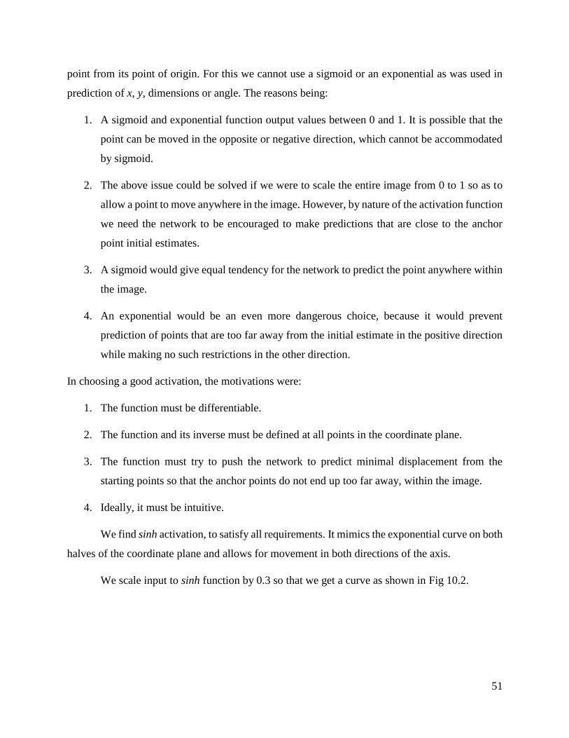
We find sinh activation, to satisfy all requirements. It mimics the exponential curve on both

halves of the coordinate plane and allows for movement in both directions of the axis.

We scale input to sinh function by 0.3 so that we get a curve as shown in Fig 10.2.

52

Fig 10.2. The activation function, sinh(x/3) used to predict the displacement of anchor points.

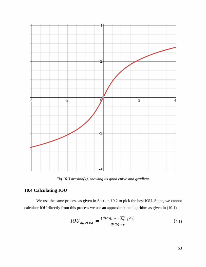
The inverse of this function is also well defined in all points of the plane as shown in Fig

4.3.

53

Fig 10.3 arcsinh(x), showing its good curve and gradient.

10.4 Calculating IOU

We use the same process as given in Section 10.2 to pick the best IOU. Since, we cannot

calculate IOU directly from this process we use an approximation algorithm as given in (10.1).

𝐼𝑂𝑈𝑎𝑝𝑝𝑟𝑜𝑥 =(𝑑𝑖𝑎𝑔𝐺.𝑇− ∑ 𝑑𝑖

4𝑖=1 )

𝑑𝑖𝑎𝑔𝐺.𝑇 (4.1)

54

We take the sum of all corresponding point distances 𝑑𝑖 between predicted point and

ground truth box corresponding point. We subtract this from the length of the diagonal of the

ground truth 𝑑𝑖𝑎𝑔𝐺.𝑇. This is scaled to one by dividing by the length of the ground truth diagonal.

We threshold this by 0.5. Anything that is equal to or higher than 0.5 is taken to be a match

while anything that is lesser is discarded.

While this is not an optimum method of calculating IOU, it is logically sound and serves

its purpose well, in determining if an object has been correctly predicted by the network.

10.5 Loss Function for Deformable Point Network

The loss function for this network includes eight different losses for all of the point

predictions. Each point prediction has two losses for x displacement prediction and y displacement

prediction.

For the loss function we use the standard square loss as shown in (10.2) and (10.3).

𝑥 𝑑𝑖𝑠𝑝𝑙𝑎𝑐𝑒𝑚𝑒𝑛𝑡 𝑙𝑜𝑠𝑠 = (𝑃𝑟𝑒𝑑𝑖𝑐𝑡𝑒𝑑 𝑥𝑑𝑖𝑠𝑝𝑙𝑎𝑐𝑒𝑚𝑒𝑛𝑡 − 𝐺𝑟𝑜𝑢𝑛𝑑 𝑇𝑟𝑢𝑡ℎ 𝑥𝑑𝑖𝑠𝑝𝑙𝑎𝑐𝑒𝑚𝑒𝑛𝑡)2 (10.2)

𝑦 𝑑𝑖𝑠𝑝𝑙𝑎𝑐𝑒𝑚𝑒𝑛𝑡 𝑙𝑜𝑠𝑠 = (𝑃𝑟𝑒𝑑𝑖𝑐𝑡𝑒𝑑 𝑦𝑑𝑖𝑠𝑝𝑙𝑎𝑐𝑒𝑚𝑒𝑛𝑡 − 𝐺𝑟𝑜𝑢𝑛𝑑 𝑇𝑟𝑢𝑡ℎ 𝑦𝑑𝑖𝑠𝑝𝑙𝑎𝑐𝑒𝑚𝑒𝑛𝑡)2 (10.3)

55

Chapter 11

Experiment Design

11.1 Motivation and Objective

The prime concern when designing experiments was to proceed by making small changes

to the network and learning from each individual modification. In the interest of ease and

simplicity, we tried to divide experiments into smaller sub-experiments. We first restricted all

experiments to only one single class of the DOTA dataset, which was small vehicles. This gave us

a training set of about 3300 images and a test set of 600 images.

The issues that we were trying to address were:

1. How does rotation affect network performance?

2. Would the addition of anchor boxes while consequently restricting rotation have any

benefits?

3. Will the ability to deform a box shape have any effect on network performance and if so in

what way?

Finally, we also wanted to set a precedent for other researchers to carry forward this work.

11.2 Training Scheme

As mentioned earlier, we started with a pretrained version of YOLO v3 for all our

experiments. The network was pretrained on MS-COCO using Darknet–54. We used a two-stage

scheme, as shown in Table 5.1 for our experiments. We first trained the last two layers of the

network for 25 epochs. We then pick the best model from these 25 epochs and then train that

model for another 15 epochs. During this second phase of training, we unfreeze all layers and

train the whole network.

We performed two sets of experiments, one with an initial batch size of 16 and another

with a batch size of 32. In both cases, the batch size for the second stage was four.

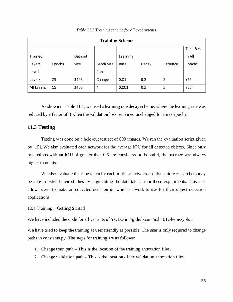
56

Table 11.1 Training scheme for all experiments.

Training Scheme

Trained

Layers Epochs

Dataset

Size Batch Size

Learning

Rate Decay Patience

Take Best

in All

Epochs

Last 2

Layers 25 3463

Can

Change 0.01 0.3 3 YES

All Layers 15 3463 4 0.001 0.3 3 YES

As shown in Table 11.1, we used a learning rate decay scheme, where the learning rate was

reduced by a factor of 3 when the validation loss remained unchanged for three epochs.

11.3 Testing

Testing was done on a held-out test set of 600 images. We ran the evaluation script given

by [15]. We also evaluated each network for the average IOU for all detected objects. Since only

predictions with an IOU of greater than 0.5 are considered to be valid, the average was always

higher than this.

We also evaluate the time taken by each of these networks so that future researchers may

be able to extend their studies by augmenting the data taken from these experiments. This also

allows users to make an educated decision on which network to use for their object detection

applications.

10.4 Training – Getting Started

We have included the code for all variants of YOLO in //github.com/axb4012/keras-yolo3.

We have tried to keep the training as user friendly as possible. The user is only required to change

paths in constants.py. The steps for training are as follows:

1. Change train path – This is the location of the training annotation files.

2. Change validation path – This is the location of the validation annotation files.

57

3. Change batch size – While the batch size for the second stage is kept constant at 4, the

initial batch size can be changed to user preference.

4. Run train.py – The input command to train would be python

11.4 Experiments with Angle

To help gain insight in how well the networks were working, we created four train and test sets:

1. Set containing objects rotated from their axes by 10 degrees to either side. We shall

call this 10-degree set.





4. Set containing all objects, irrespective of rotation.

It should be noted that even though, theoretically the 45-degree set must encompass all objects, it

does not because of artifacts in annotation as described in the later sections.

11.5 Experiments with YOLO v3

We test YOLO v3 on all four sets. Additionally, we also present results for non-oriented

experiments on YOLO v3. This is so that we set a baseline result on YOLO v3. By this experiment

we take the minimum x, y and maximum x, y coordinated of the ground truth points as object

labels.

11.6 Experiments on YOLO Rotated

We train three variants of the YOLO Rotated network:

1. Anchor boxes only allowed to rotate by 10 degrees to either side of the network. We shall

call this 10-degree network.



58



All three variants of the network are tested on all four test sets. We present results and conclusions

in the next sections.

11.7 Experiments on YOLO Extra Anchors

We test the YOLO Extra Anchors network on all four datasets and present results in the

next chapter. All hyperparameters remain unchanged. The freedom of rotation or wiggle to each

side from axis is 22.5 degrees.

11.8 Experiments on Deformable YOLO

Just like YOLO Extra Anchors, we test Deformable YOLO on all four-test set and present

results in the coming sections.

11.9 Results of Experiments

We have tabulated the results of YOLO v3 as well as its variants in Table 11.2 and Table

11.3. Table 11.1 is the version that was training on an initial batch size of 16 while Table 11.3 has

results from the 32-batch version. We only found marginal improvements in using a batch size of

32 for best cases in each set.

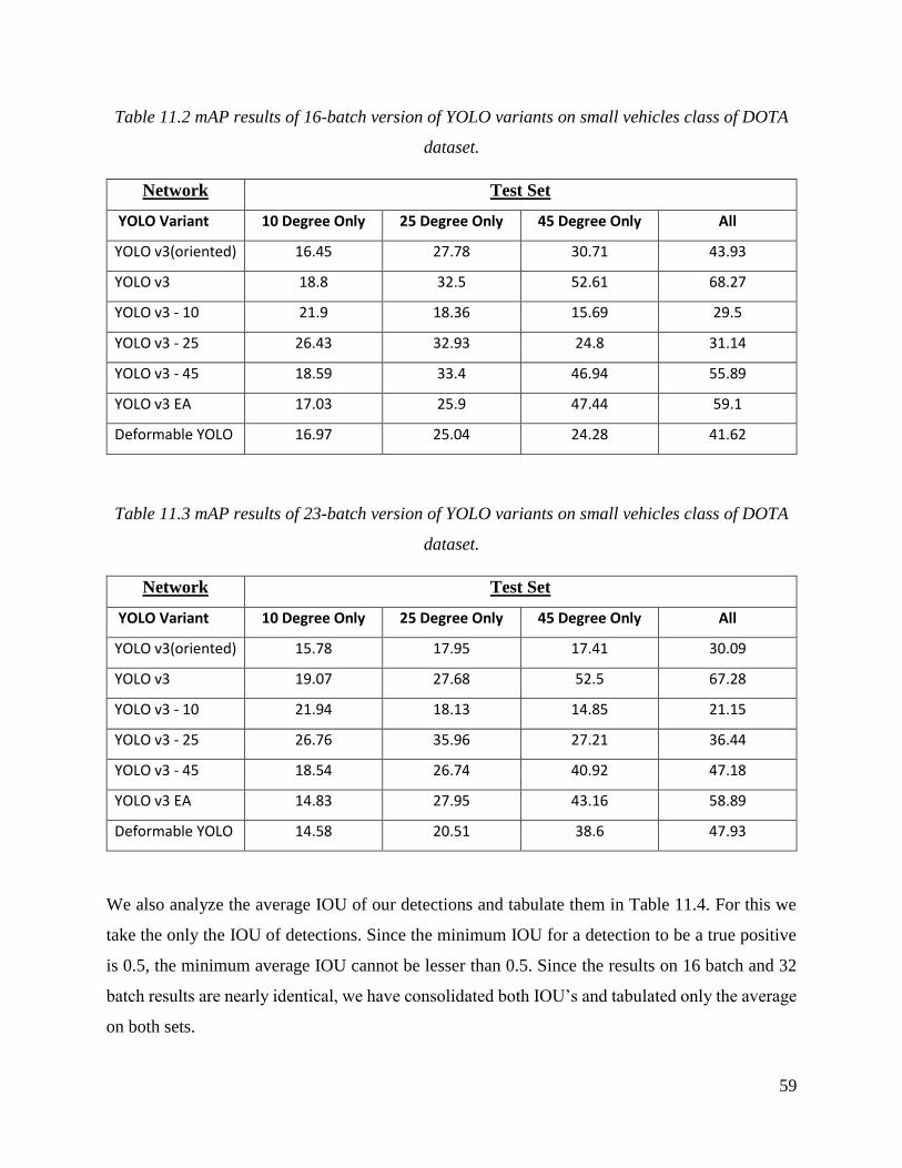
59

Table 11.2 mAP results of 16-batch version of YOLO variants on small vehicles class of DOTA

dataset.

Network Test Set

YOLO Variant 10 Degree Only 25 Degree Only 45 Degree Only All

YOLO v3(oriented) 16.45 27.78 30.71 43.93

YOLO v3 18.8 32.5 52.61 68.27

YOLO v3 - 10 21.9 18.36 15.69 29.5

YOLO v3 - 25 26.43 32.93 24.8 31.14

YOLO v3 - 45 18.59 33.4 46.94 55.89

YOLO v3 EA 17.03 25.9 47.44 59.1

Deformable YOLO 16.97 25.04 24.28 41.62

Table 11.3 mAP results of 23-batch version of YOLO variants on small vehicles class of DOTA

dataset.

Network Test Set


YOLO v3(oriented) 15.78 17.95 17.41 30.09

YOLO v3 19.07 27.68 52.5 67.28

YOLO v3 - 10 21.94 18.13 14.85 21.15

YOLO v3 - 25 26.76 35.96 27.21 36.44

YOLO v3 - 45 18.54 26.74 40.92 47.18

YOLO v3 EA 14.83 27.95 43.16 58.89

Deformable YOLO 14.58 20.51 38.6 47.93

We also analyze the average IOU of our detections and tabulate them in Table 11.4. For this we

take the only the IOU of detections. Since the minimum IOU for a detection to be a true positive

is 0.5, the minimum average IOU cannot be lesser than 0.5. Since the results on 16 batch and 32

batch results are nearly identical, we have consolidated both IOU’s and tabulated only the average

on both sets.

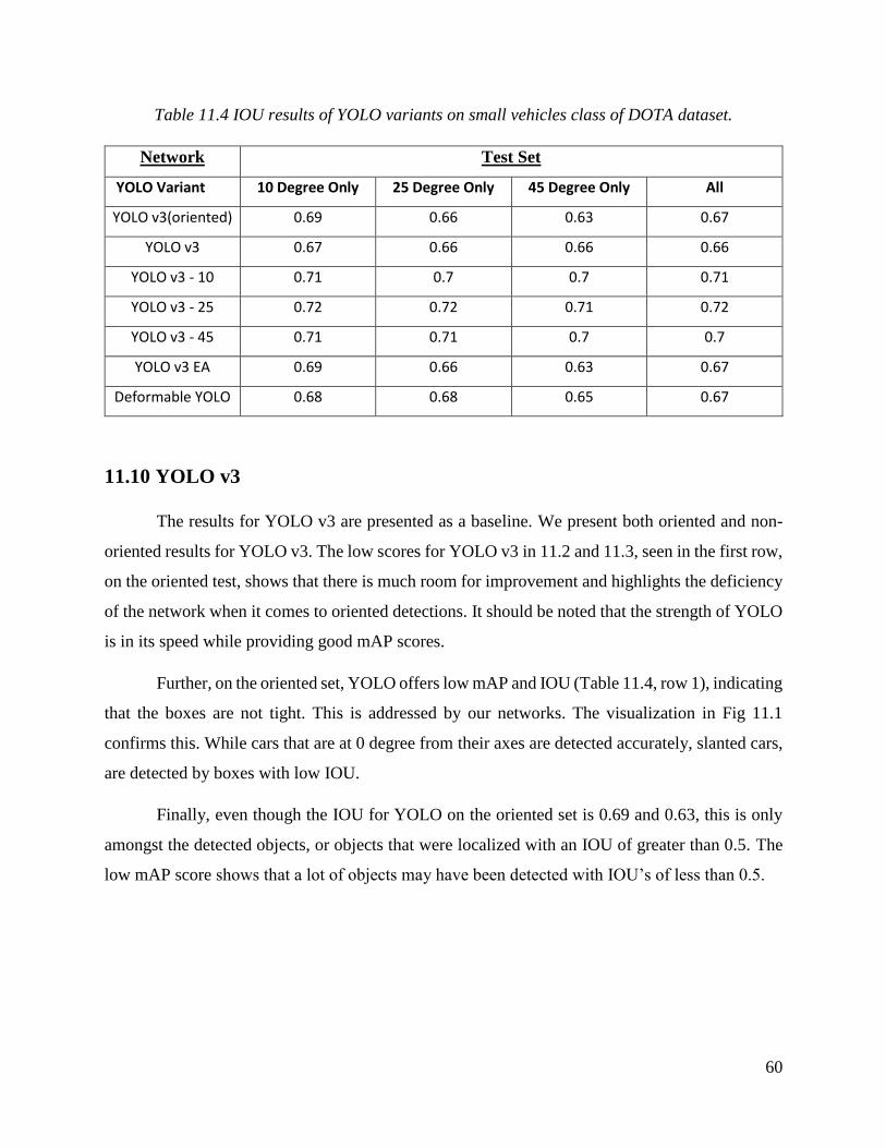
60

Table 11.4 IOU results of YOLO variants on small vehicles class of DOTA dataset.

Network Test Set


YOLO v3(oriented) 0.69 0.66 0.63 0.67

YOLO v3 0.67 0.66 0.66 0.66

YOLO v3 - 10 0.71 0.7 0.7 0.71

YOLO v3 - 25 0.72 0.72 0.71 0.72

YOLO v3 - 45 0.71 0.71 0.7 0.7

YOLO v3 EA 0.69 0.66 0.63 0.67

Deformable YOLO 0.68 0.68 0.65 0.67

11.10 YOLO v3

The results for YOLO v3 are presented as a baseline. We present both oriented and non-

oriented results for YOLO v3. The low scores for YOLO v3 in 11.2 and 11.3, seen in the first row,

on the oriented test, shows that there is much room for improvement and highlights the deficiency

of the network when it comes to oriented detections. It should be noted that the strength of YOLO

is in its speed while providing good mAP scores.

Further, on the oriented set, YOLO offers low mAP and IOU (Table 11.4, row 1), indicating

that the boxes are not tight. This is addressed by our networks. The visualization in Fig 11.1

confirms this. While cars that are at 0 degree from their axes are detected accurately, slanted cars,

are detected by boxes with low IOU.

Finally, even though the IOU for YOLO on the oriented set is 0.69 and 0.63, this is only

amongst the detected objects, or objects that were localized with an IOU of greater than 0.5. The

low mAP score shows that a lot of objects may have been detected with IOU’s of less than 0.5.

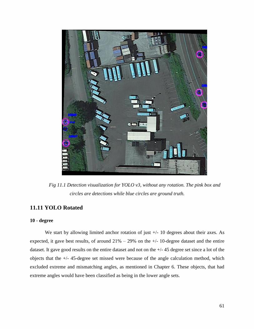
61

Fig 11.1 Detection visualization for YOLO v3, without any rotation. The pink box and

circles are detections while blue circles are ground truth.

11.11 YOLO Rotated

10 - degree

We start by allowing limited anchor rotation of just +/- 10 degrees about their axes. As

expected, it gave best results, of around 21% – 29% on the +/- 10-degree dataset and the entire

dataset. It gave good results on the entire dataset and not on the +/- 45 degree set since a lot of the

objects that the +/- 45-degree set missed were because of the angle calculation method, which

excluded extreme and mismatching angles, as mentioned in Chapter 6. These objects, that had

extreme angles would have been classified as being in the lower angle sets.

62

Fig 11.2 Detection visualization for YOLO v3, with +/- 10-degree rotation. The pink

boxes are detections while blue circles are ground truth. Note the mistaken identifications which

contributed to low scores.

25 - degree

The 25-degree set performed like the 10 – degree set giving best results in +/- 25 degree

and the entire dataset. The best mAP that we observed was on 32 batch model, on the entire dataset.

We observed a mAP score of around 36.44%. One of the most positive conclusions from the results

is that the mAP scores seem to be improving with increasing angle of freedom of rotation. The

increases by 1%, but this is accompanied by a strong rise in mAP scores. This indicates an overall

better detector. In Fig 11.3, we see that the network was able to detect objects that were rotated by

+/- 25 degrees. It also made a few false detections; however, this was because it generalized

rotations close to but out of range of +/- 25 degrees as being within range. This shows that our

network generalizes well with the dataset provided.

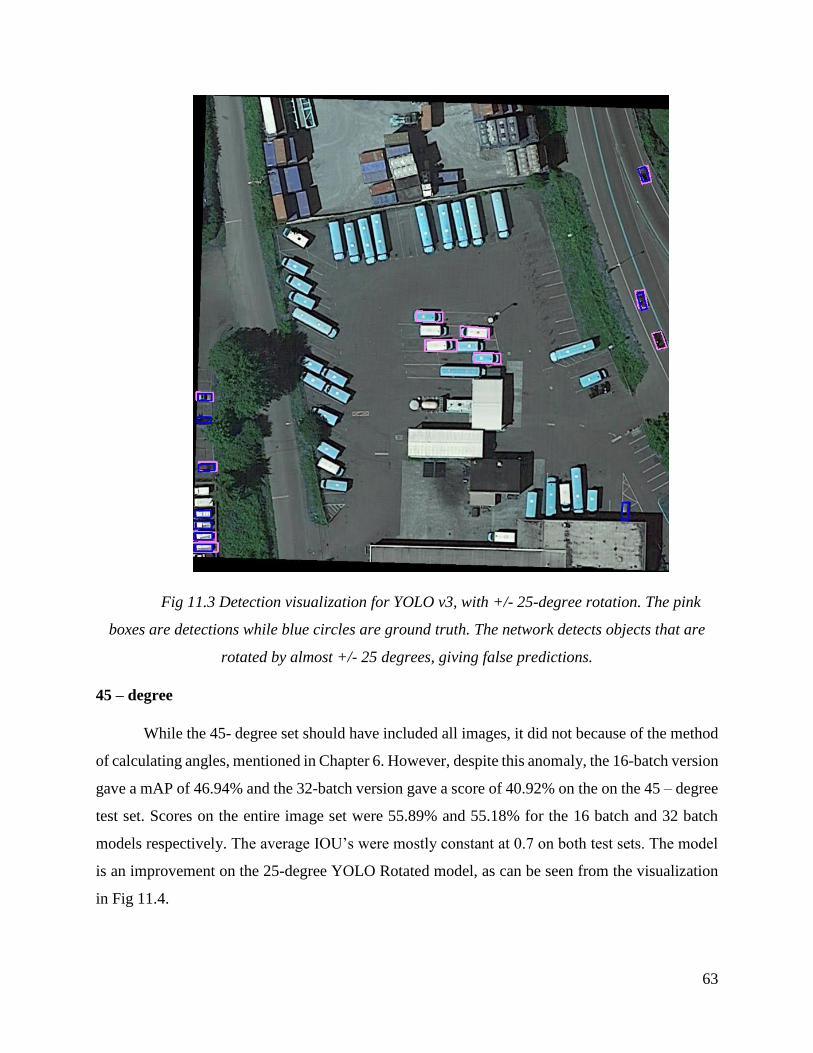
63


boxes are detections while blue circles are ground truth. The network detects objects that are

rotated by almost +/- 25 degrees, giving false predictions.

45 – degree

While the 45- degree set should have included all images, it did not because of the method

of calculating angles, mentioned in Chapter 6. However, despite this anomaly, the 16-batch version

gave a mAP of 46.94% and the 32-batch version gave a score of 40.92% on the on the 45 – degree

test set. Scores on the entire image set were 55.89% and 55.18% for the 16 batch and 32 batch

models respectively. The average IOU’s were mostly constant at 0.7 on both test sets. The model

is an improvement on the 25-degree YOLO Rotated model, as can be seen from the visualization

in Fig 11.4.

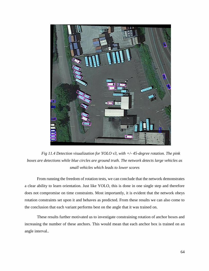
64


boxes are detections while blue circles are ground truth. The network detects large vehicles as

small vehicles which leads to lower scores

From running the freedom of rotation tests, we can conclude that the network demonstrates

a clear ability to learn orientation. Just like YOLO, this is done in one single step and therefore

does not compromise on time constraints. Most importantly, it is evident that the network obeys

rotation constraints set upon it and behaves as predicted. From these results we can also come to

the conclusion that each variant performs best on the angle that it was trained on.

These results further motivated us to investigate constraining rotation of anchor boxes and

increasing the number of these anchors. This would mean that each anchor box is trained on an

angle interval..

65

11.12 YOLO – Extra Anchors

Our intuition of adding more anchor boxes while restricting rotation, clearly produces

positive results. Table 11.2 and 11.3, row 6 show that mAP scores on the entire dataset improves

by about 4% on the 16-batch set and 11% on the 32-batch set, when compared to the 45 – degree

model on the row 5 of both tables. This is a clear indication of the robustness of the model as well

as the concept of restricted rotation while adding extra anchor boxes. We can see that the best

network offers a mAP score 59.1 % as compared to a non-oriented score of 68.2 %. Such a drop

is to be expected as the network has more parameters to learn and is also a more complicated

architecture.

Although mAP scores are lower, inspection of output images shows that including angle

prediction leads to better quality of results. Further the average IOU changes minimally from the

other sets, as seen in Table 11.4. A constant IOU with a steady improvement in mAP in a clear

indication of an improved model.

66

Fig 11.5 Detection visualization for YOLO v3 Extra Anchors. The pink boxes are

detections while blue circles are ground truth. The network accurately detects objects of all

rotations.

11.13 Deformable YOLO

To further augment our results, we also train and test a deformable model that uses anchor

boxes that can change shape without restriction. This allows location and detection of objects that

are not strictly rectangular. We see, from Table 11.3 and 11.4, row 7 that while mAP scores are

certainly lower than that of the Extra Anchors model, results are competitive. We can a mAP score

of 41.62% on the 16-batch model and 47.93% on the 32-batch model when tested on the entire

dataset. This model would prove to be more useful for objects that are of non-rectangular shapes.

It offers a compromise between pixel wise segmentation and speed. We do observe, from Table

67

11.5, row 7 that the IOU is 0.67, which is comparable with YOLO Extra Anchors. The

visualizations in Fig 11.3 provide better information about the model, since we see that the boxes

predicted are deformable. They can change to irregular four-point shapes and are not restricted

like our previous models. We can conclude that the best deformable model, which is the 32-batch

model gives a mAP score of 47.93% is only beaten by the Extra Anchors model which has a mAP

score of 58.89%.

Fig 11.6 Detection visualization for Deformable YOLO. The pink boxes are detections

while blue circles are ground truth. The network predictions are not restricted to rectangles or

squares as can be seen in the top right car images.

68

11.14 Time Sensitivity

One of the best features of YOLO is its time sensitivity. Our models are the first to

incorporate rotation and deformable points into YOLO.

We trained our models on a 12 core Intel Xeon CPU E5-2650 v4. The 16-batch models

were trained on an NVIDIA Tesla M40 with 24 GB of memory. The 32-batch models were trained

on an NVIDIA V100 with 32 GB of memory. The 16-batch models took about 12 hours to train

on a subset of the DOTA dataset size which had 3300 images of 832 × 832. The 32-batch models

took around 7 hours to train on the same dataset.

For testing, we used an Intel Xeon CPU E5-2623 with 4 cores and an NVIDIA Tesla P100

GPU with 12 GB of memory. We have listed our testing times in Table 11.5 and 11.6.

As of February 2019, ours is the only model that offers angle or deformity in predictions

at speeds comparable to YOLO v3.

Table 11.5 Time analysis for 16-batch models.

Network FPS

YOLO v3 9.931

YOLO v3 - 10 9.686

YOLO v3 - 25 10.355

YOLO v3 - 45 10.706

YOLO v3 Extra Anchors 9.638

Deformable YOLO v3 9.54

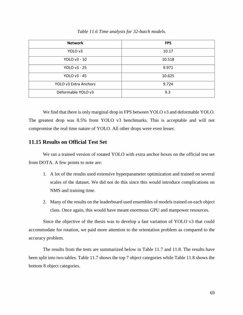
69

Table 11.6 Time analysis for 32-batch models.

Network FPS

YOLO v3 10.17

YOLO v3 - 10 10.518

YOLO v3 - 25 9.971

YOLO v3 - 45 10.625

YOLO v3 Extra Anchors 9.724

Deformable YOLO v3 9.3

We find that there is only marginal drop in FPS between YOLO v3 and deformable YOLO.

The greatest drop was 8.5% from YOLO v3 benchmarks. This is acceptable and will not

compromise the real time nature of YOLO. All other drops were even lesser.

11.15 Results on Official Test Set

We ran a trained version of rotated YOLO with extra anchor boxes on the official test set

from DOTA. A few points to note are:

1. A lot of the results used extensive hyperparameter optimization and trained on several

scales of the dataset. We did not do this since this would introduce complications on

NMS and training time.

2. Many of the results on the leaderboard used ensembles of models trained on each object

class. Once again, this would have meant enormous GPU and manpower resources.

Since the objective of the thesis was to develop a fast variation of YOLO v3 that could

accommodate for rotation, we paid more attention to the orientation problem as compared to the

accuracy problem.

The results from the tests are summarized below in Table 11.7 and 11.8. The results have

been split into two tables. Table 11.7 shows the top 7 object categories while Table 11.8 shows the

bottom 8 object categories.

70

Table 11.7 Results on DOTA Test Set – Top Performers.

Class Small

Vehicle Plane

Tennis

Court Ship

Tank Large

Vehicle Pool

mAP

Score

0.63 0.62 0.6 0.54 0.45 0.4 0.33

Table 11.8 Results on DOTA Test Set – Bottom Performers.

Class Roundabout Harbor Baseball

Diamond Bridge

Soccer

Field

Track

Field Helicopter

Basketball

Court

mAP

Score

0.21 0.18 0.1 0.06 0.03 0.03 0.01 0.004

While the results of the top performers are satisfactory, the bottom performers seem

extremely low in comparison. From visual observation we postulate that this is because of the

scarcity of these objects in the train set as well as the test set. For example, the training set had

more than 30,000 large vehicles but only about 500 examples of helicopters.

Further, in many examples the detector gave inaccurate rotations as compared to the labels.

An example is given in Fig 11.7 where the pink box shows the detection while the blue box shows

the ground truth. In this case, even though the object was detected accurately, the scores would be

penalized since it does not match the ground truth.

71

Fig 11.7 Examples of cases where the model results were penalized based on arbitrary rotation.

We also believe that the huge variations in scale also contributed to poor detection. We

found that in some examples, the size of an object spanned almost 800 pixels wide, in a 832 × 832

input image. An example of this is shown in Fig 11.8 where the baseball diamond spans almost

the whole image. This can be solved by using multi-scale input as in [33]. We have included this

in our future work.

Fig 11.8 A baseball diamond that spans across almost the whole image. In this case the object

will not be detected because of its sheer size.

72

Finally, there are also severe variations in size of objects. In Fig 11.8 the cars on the left

tile is undetected. However, those the right panel is detected by the network. A zoomed version of

Fig 11.9 (left) is presented in Fig 11.10. Here it is seen that several cars are not labelled (circled in

red.).

Fig 11.9 In the left, the cars are too small to be detected. The network struggles with such

examples where the object sizes vary from a few pixels to a 20-30 pixels, as in the right.

Fig 11.10 The cars in blue are labelled. Those in red have been missed by the annotators. Such

inconsistencies might have contributed to false detections by the network.

73

Chapter 12

Conclusions and Future Work

12.1 Conclusions and Future Work

We see this as the apparent future direction of object detection. There are many regions of

improvement for the networks that we have proposed, and we hope to see research in these areas.

Some of the main areas of improvement are:

mAP Scores – The scores from the best rotation model that we had was 59.1% while the

YOLO v3 baseline was 68.27%. This is a large gap and we believe that this is one the main

shortcomings of our network. We feel that this could be largely due to our method of training

where we train it for object localization, shape regression and angle regression altogether. A

decoupled version of training might help boost mAP scores.

Within the dataset itself, we observed that the objects were of different scales. While

YOLO v3 does account for this, we believe that it could be improved. To highlight the variation

in height and width of small vehicles in the DOTA dataset, we have plotted a height vs width chart

in Fig 12.1.

Our anchor boxes struggled to keep up with this huge variation. To overcome this, we could

have used extra scales or an inception [34] type of network, with multiple scales of convolution.

We also explored the suggestion of using more anchor boxes at different sizes however,

deemed this too complicated to finish within the time frame.

Overall, even though, we believe that the network did give good results and mAP scores,

there is a lot of room for improvement in this area.

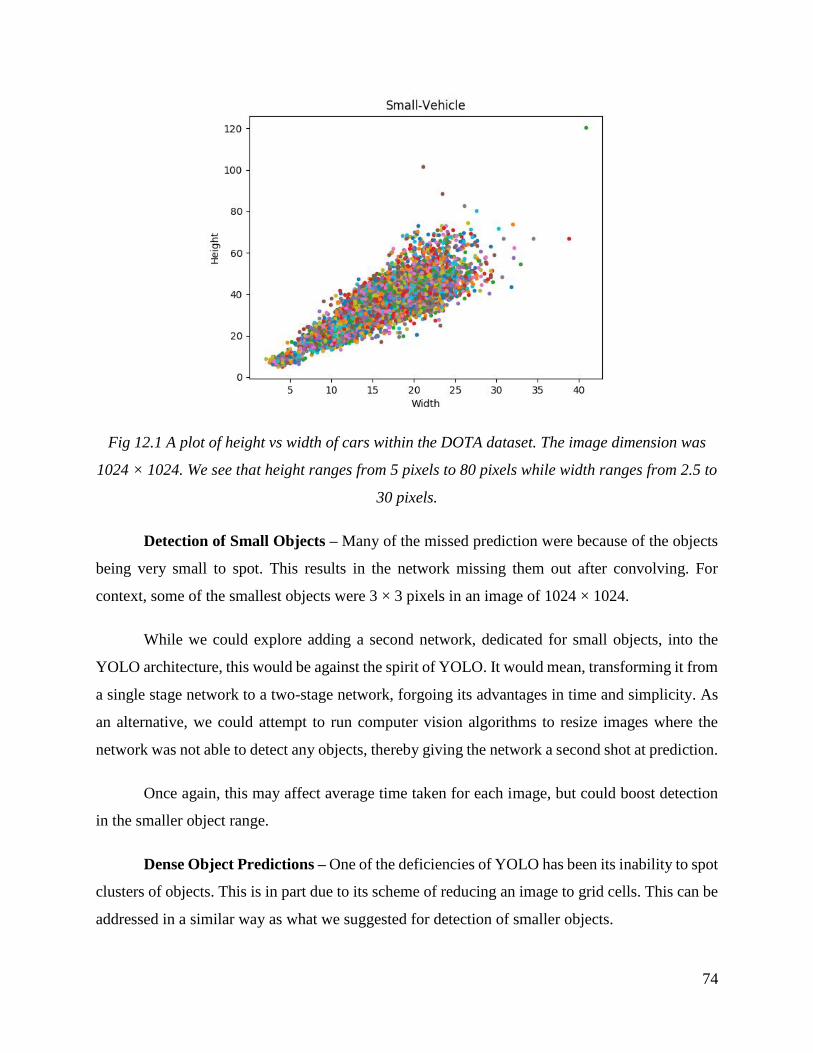
74

Fig 12.1 A plot of height vs width of cars within the DOTA dataset. The image dimension was

1024 × 1024. We see that height ranges from 5 pixels to 80 pixels while width ranges from 2.5 to

30 pixels.

Detection of Small Objects – Many of the missed prediction were because of the objects

being very small to spot. This results in the network missing them out after convolving. For

context, some of the smallest objects were 3 × 3 pixels in an image of 1024 × 1024.

While we could explore adding a second network, dedicated for small objects, into the

YOLO architecture, this would be against the spirit of YOLO. It would mean, transforming it from

a single stage network to a two-stage network, forgoing its advantages in time and simplicity. As

an alternative, we could attempt to run computer vision algorithms to resize images where the

network was not able to detect any objects, thereby giving the network a second shot at prediction.

Once again, this may affect average time taken for each image, but could boost detection

in the smaller object range.

Dense Object Predictions – One of the deficiencies of YOLO has been its inability to spot

clusters of objects. This is in part due to its scheme of reducing an image to grid cells. This can be

addressed in a similar way as what we suggested for detection of smaller objects.

75

We could also consider changing the architecture entirely, but this would once again, be a

completely different network instead of an improvement of an existing method.

12.2 Computer Vision in Object Detection

We also briefly explored using basic sharpening filters in testing of our dataset. We found

marginal improvement of about 0.5%. It should be mentioned that a lot of networks benefit from

such computer vision methods This could certainly be another area of research where influences

of computer vision could be tested on YOLO network and its variants.

Apart from sharpening filters, we could also try using changing tone scale, changing color

or using images with non-linear functions applied based on color and location of pixels.

12.3 Conclusion

Through this thesis, we offer the culmination of months of research and hard work. We

present three variants of YOLO, giving tight box predictions that are agnostic to shape and

orientation. We show that the network can learn to predict angle along with location and

dimensions of objects in an image with minimal compromises on time taken to run the network.

We also present baseline for a model that can change its shape to irregular geometry, offering

better object detection with datasets of objects that are not strictly rectangular. We show that the

accuracy scores of all these variants are very competitive to the original YOLO network,

minimizing tradeoffs. We believe that this could be very beneficial to areas of surveillance, defense

and tracking. Despite this, we hope that the work presented here is used for the benefit of human

kind and is used to improve quality of life and progress research in deep learning.

76

References

[1] J. Redmon, S. Divvala, R. Girshik and F. Ali, "You Only Look Once: Unified, Real-Time Object

Detection," in Computer Vision and Pattern Recognition, 2015.

[2] tejaslodaya, "www.github.com," Github, 8 July 2018. [Online]. Available:

https://github.com/tejaslodaya/car-detection-yolo/blob/master/README.md. [Accessed 17 January

2019].

[3] J. Redmon and A. Farhadi, " YOLO9000: better, faster, stronger," in Computer Vision and Pattern

Recognition, 2017.

[4] C. Zhang, "Gentle guide on how YOLO Object Localization works with Keras (Part 2),"

heartbeat.fritz.ai, 27 March 2018. [Online]. Available: https://heartbeat.fritz.ai/gentle-guide-on-

how-yolo-object-localization-works-with-keras-part-2-65fe59ac12d. [Accessed February 2019].

[5] E. Mark, V. G. Luc, K. I. W. Christopher, W. John and Z. Andrew, "The Pascal Visual Object

Classes (VOC) Challenge," International Journal of Computer Vision, vol. 88, no. 2, pp. 303-308,

2010.

[6] Aphex34, "Wikipedia," 16 December 2015. [Online]. Available:

https://commons.wikimedia.org/w/index.php?curid=45679374. [Accessed 2019].

[7] T.-Y. Lin, M. Maire, S. Belongie, J. Hays, P. Perona, D. Ramanan, P. Dollar and C. L. Zitnick,

"Microsoft COCO: Common Objects in Context," in European Conference on Computer Vision,

Zurich, 2014.

[8] R. Girshick, J. Donahue, T. Darrell and J. Malik, "Rich feature hierarchies for accurate object

detection and semantic segmentation," 22 October 2014. [Online]. Available: arXiv:1311.2524

[cs.CV].

[9] G. Ross, "Fast R-CNN," in Computer Vision and Pattern Recognition, 2015.

[10] S. Ren, K. He, R. Girshick and J. Sun, "Faster R-CNN: Towards Real-Time Object Detection with

Region Proposal Networks," in Computer Vision and Pattern Recognition, 2015.

[11] K. He, G. Gkioxari, D. Piotr and R. Girshik, "Mask R-CNN," 24 January 2018 . [Online].

Available: https://arxiv.org/abs/1703.06870.

[12] J. Redmon and A. Farhadi, "YOLOv3: An Incremental Improvement," 8 April 2018. [Online].

Available: arXiv:1804.02767 [cs.CV].

[13] W. Liu, D. Anguelov, D. Erhan, C. Szegedy, S. Reed, C.-Y. Fu and A. C. Berg, "SSD: Single Shot

MultiBox Detector," 29 December 2016. [Online]. Available: Computer Vision and Pattern

Recognition (cs.CV).

77

[14] Y. Zhou, Q. Ye, Q. Qiang and J. Jianbin, "Oriented Response Networks," 13 July 2017. [Online].

Available: arXiv:1701.01833 [cs.CV].

[15] D. Ni and Z. Chang, "DOTA: A Large-scale Dataset for Object Detection in Aerial Images -

Results," 2018. [Online]. Available: https://captain-whu.github.io/DOTA/results.html.

[16] G.-S. Xia, B. Xiang, D. Jian, Z. Zhen, S. Belongie, J. Luo, M. Datcu, M. Pelillo and L. Zhang,

"DOTA: A Large-scale Dataset for Object Detection in Aerial Images," 27 January 2018. [Online].

Available: Computer Vision and Pattern Recognition (cs.CV).

[17] L. Liu, Z. Pan and L. Bin, "Learning a Rotation Invariant Detector with Rotatable Bounding Box,"

26 Novemeber 2017. [Online]. Available: arXiv:1711.09405 [cs.CV].

[18] K. Simonyan and A. Zisserman, "Very deep convolutional networks for large-scale image

recognition," in Computer Vision and Pattern Recognition, 2014.

[19] M. A. Sadeghi and D. Forsyth, "30hz object detection with dpm v5," in European Conference on

Computer Vision, Cham, 2014.

[20] J. Yan, Z. Lei, L. Wen and S. Z. Li, "The Fastest Deformable Part Model for Object Detection," in

IEEE Conference on Computer Vision and Pattern Recognition, Columbus, 2014.

[21] P. Sharma, "www.analyticsvidhya.com," analyticsvidhya, 6 December 2018. [Online]. Available:

https://www.analyticsvidhya.com/blog/2018/12/practical-guide-object-detection-yolo-framewor-

python/. [Accessed 17 January 2019].

[22] J. Deng, W. Dong, R. Socher, L.-J. Li, K. Li and L. Fei-Fei, "ImageNet: A large-scale hierarchical

image database," in IEEE Conference on Computer Vision and Pattern Recognition, Miami, 2009.

[23] K. H. He, Z. Xiangyu, R. Shaoqing and S. Jian, "Deep residual learning for image recognition,"

arXiv:1512.03385 [cs.CV], 10 December 2015.

[24] L. Wei, A. Dragomir, D. Erhan, S. Christian, R. Scott, F. Cheng-Yang and C. B. Alexander, "SSD:

Single Shot MultiBox Detector," arXiv:1512.02325v5 [cs.CV], 29 December 2016.

[25] G. A. Miller, "WordNet: a lexical database for English," Communications of the ACM, pp. 39-41,

1995.

[26] Tesla, "Tesla Model S," Tesla Inc, January 2019. [Online]. Available:

https://www.tesla.com/models. [Accessed 21 January 2019].

[27] Waymo, "Our Journey," Waymo, January 2019. [Online]. Available: https://waymo.com/journey/.

[Accessed 21 January 2019].

[28] D. Silver, "How the Udacity Self-Driving Car Works," Medium, 6 September 2017. [Online].

Available: https://medium.com/udacity/how-the-udacity-self-driving-car-works-575365270a40.

[Accessed 23 January 2019].

78

[29] A. Hawkjins, "GM will make an autonomous car without steering wheel or pedals by 2019," The

Verge, 12 January 2018. [Online]. Available: https://www.theverge.com/2018/1/12/16880978/gm-

autonomous-car-2019-detroit-auto-show-2018. [Accessed 21 January 2019].

[30] E. Johnson, "Full Q&A: Tesla and SpaceX CEO Elon Musk on Recode Decode," recode.net, 5

Novemeber 2018. [Online]. Available: https://www.recode.net/2018/11/2/18053428/recode-decode-

full-podcast-transcript-elon-musk-tesla-spacex-boring-company-kara-swisher. [Accessed 21

January 2019].

[31] N. Levy, "Second Amazon Go store opens in Seattle with further expansion on the horizon,"

geekwire, 27 August 2018. [Online]. Available: https://www.geekwire.com/2018/second-amazon-

go-store-opens-seattle-expansion-horizon/. [Accessed 21 January 2019].

[32] J. Long, E. Shelhamer and D. T. Trevor, "Fully convolutional networks for semantic segmentation,"

in IEEE Conference on Computer Vision and Pattern Recognition, Boston, 2015.

[33] B. G. Bai. Yancheng, "Multi-scale Fully Convolutional Network for Face Detection in the Wild,"

Conference on Computer Vision and Pattern Recognition Workshops (CVPRW), pp. 2078-2087,

2017.

[34] L. W. J. Y. S. P. R. S. A. D. E. D. V. V. R. A. Szegedy Christian, "Going Deeper with

Convolutions," 17 September 2014. [Online]. Available: arXiv:1409.4842. [Accessed 2019].

[35] B. G. Bai. Yancheng, "Multi-scale Fully Convolutional Network for Face Detection in the Wild,"

IEEE Conference on Computer Vision and Pattern Recognition Workshops (CVPRW), pp. 2078-

2087, 2017.

79

Appendix

As much as possible, we have tried to ensure that minimal changes need to be done to run

the experiment. We have made sure that all data preparation is done within the training and testing

pipeline itself. All scripts have been changed to work with the DOTA dataset as of 08/12/2019.

In the following sections we will summarize how to train, test and visualize our models on

the DOTA set.

Data

The data is uploaded at https://captain-whu.github.io/DOTA/dataset.html. The training set

and validation set consist of a folder containing .jpg files and a corresponding folder with .txt files

containing the labels. We recommend that no changes be done to these files. As of 08/12/2019,

the labels must be of the form “x1, y1, x2, y2, x3, y3, x4, y4, category, difficult”.

Data Preparation

For data preparation and cropping of images of required size, we recommend using the

official DOTA API at https://github.com/CAPTAIN-WHU/DOTA_devkit. The instructions on how to

run this API can be found on the github link provided. As mentioned before it is assumed that the

code commit from 08/12/2019 is used for this purpose.

The output of the cropping function would look very similar to the initial structure. We

expect two folders, one for .jpg files and the other for .txt files. In out experiments, we had close

to 30,000 training images.

Running YOLO

Our code is based off https://github.com/qqwweee/keras-yolo3. The code has been uploaded

to https://github.com/axb4012/keras-yolo3. To accommodate for data format, our script uses its own

data manipulation operation included in yolo3/utils.py. We have also made necessary changed to

model_data/dota_classes.txt and model_data/yolo_anchors.txt to suit our dataset.

For the purpose of training, the user is expected to make changes to train.py – lines 17 –

20. The included folder logs/user_defined_model_path will hold the trained model files as well

https://captain-whu.github.io/DOTA/dataset.html

https://github.com/CAPTAIN-WHU/DOTA_devkit

https://github.com/qqwweee/keras-yolo3

https://github.com/axb4012/keras-yolo3

80

as the checkpoints. Training typically takes about 5 hours on an NVIDIA Titan Xp for 25 epochs.

We recommend 25 epochs since this has shown the best results on the validation set.

Testing YOLO

We expect the test set to be placed in a folder with .jpg files. The folder can have as many

images as the user requires. The user is expected to run run_oriented_test.py --model_name --

anchors_path --output_folder_path --output_folder_path --image_size. The script saves all

results in the user defined folder output_folder_path. The results will a set of 15 files with formats

as defined by https://captain-whu.github.io/DOTA/tasks.html. This is so that the user may upload

the files directly to the evaluation server for testing.

Visualizing YOLO

In addition to testing we expect that the user may want to visualize results on images. Once

again, the user is expected to have all required images in a folder as .jpg files. The user needs to

run run_visuals_dota.py--model_name --anchors_path --input_folder_path --

output_folder_path --image_size. The script will write .jpg files to output_folder_path which

is a user defined folder. The predictions will be shown as boxes around the detected objects.

Closing Notes

We have also included detailed instructions on the github page for the project. The DOTA

dataset is expected to change in annotation quality and dataset size however, so far, the format has

remained unchanged. For support or questions, we have included the contact information of the

author as well as the primary advisor.

Author: Aneesh Bhat

Email: [email protected]

Advisor: Raymond Ptucha

Email: [email protected]

https://captain-whu.github.io/DOTA/tasks.html

Aerial Object Detection using Learnable Bounding Boxes

Documents

Transcript of Aerial Object Detection using Learnable Bounding Boxes