AER repex modelling - Australian Energy Regulator - TN081...Our assessment approach has used the...
31
AER repex modelling Assessing TasNetworks’ replacement forecast A report to TasNetworks Confidential final January 2016
-
Upload
phungkhanh -
Category
Documents
-
view
215 -
download
0
Transcript of AER repex modelling - Australian Energy Regulator - TN081...Our assessment approach has used the...

AER repex modelling Assessing TasNetworks’ replacement forecast
A r e p o r t t o T a s N e t w o r k s
C o n f i d e n t i a l f i n a l
J a n u a r y 2 0 1 6

Table of contents
Executive Summary............................................................................... 4
Introduction 4
Assessment findings 4
1 Introduction ........................................................................... 6
1.1 Background and scope 6
1.2 Nuttall Consulting experience in this task 7
1.3 Key information sources 7
1.4 Structure 7
2 Assessment approach ............................................................ 9
2.1 AER assessment approach 9 2.1.1 The repex component assessed through the model 9 2.1.2 Defining the reasonable bound 10
2.2 Our assessment approach 10 2.2.1 Assessment period 10 2.2.2 Repex component modelled 11 2.2.3 Model studies assessed 11 2.2.4 Calibration volume sensitivity scenario 12
3 Repex forecast assessment .................................................. 13
3.1 Repex model results and discussion 13
3.2 Summary and conclusions 15
A TasNetworks repex model development ............................. 16
A.1. The AER’s repex model 16 A.1.1. Overview of repex model 16 A.1.2. AER repex model form, inputs and output 16 A.1.3. Model planning parameter calibration 17
A.2. TasNetworks repex model 19 A.2.1. TasNetworks repex model structure set up 19 A.2.2. Model calibration set up 19 A.2.3. Adjustments to data and calibration 20 A.2.4. Model calibration process 20 A.2.5. Alterations to the published AER model 21
B Calibration volume sensitivity scenario ................................ 22
B.1. Considerations for scenario 22
B.2. Scenario calibration volume assumptions 22
B.3. Scenario model results and discussion 23
C Assessing forecast differences ............................................. 26
C.1. Overview of assessment approach 26
C.2. Results of assessment 26 C.2.1. Poles 27 C.2.2. Overhead conductors 28 C.2.3. Underground cables 28 C.2.4. Services 29

Nuttall Consulting
C.2.5. Transformers 29 C.2.6. Switchgear 30
C.3. Summary and conclusions 31
Nuttall Consulting does not take responsibility in any way whatsoever to any person or organisation other than TasNetworks Distribution in respect of information set out in this
document, including any errors or omissions therein, arising through negligence or otherwise.

Nuttall Consulting
Nuttall Consulting Repex modelling report Page 4
Executive Summary
Introduction
Nuttall consulting has been engaged by Tasmanian Networks Pty Ltd (TasNetworks) to undertake an
assessment of its replacement expenditure (repex) forecast. This assessment must use the predictive
model that the Australian Energy Regulator (AER) has indicated it will use as part of its assessment
process. This model is called the AER repex model.
We have used asset age profiles and asset replacement data reported in various TasNetworks
Regulatory Information Notices (RIN) to prepare this model. This preparation has been supported by
other data provided by TasNetworks and other comments and advice provided during the course of
two workshops with relevant TasNetworks personnel.
We have been able to assess approximately 69% of TasNetworks’ repex forecast using this model1.
We have used various AER documents to guide our assessment approach, including its expenditure
assessment guideline, its repex model manual, and most importantly, its recent determinations.
Our assessment approach has used the method the AER applies to determine a reasonable repex
forecast. Using this approach, we have assessed TasNetworks forecast over two time periods:
the five-year period commencing at the start of TasNetworks’ next regulatory period (2017/18
to 2021/22) – we believe this longer period is a more reliable length for assessments through
the repex model
the two-year period covering TasNetworks’ next regulatory period (2017/18 to 2018/19).
To support the assessment, we have also undertaken a number of additional studies.
Assessment findings
Our assessment using the AER’s repex model supports TasNetworks’ repex forecast.
Our application of the AER’s assessment method provides very strong support to TasNetworks’
forecast:
TasNetworks’ forecast over the five-year assessment period is significantly below all the key
studies considered by the AER, ranging between 54% and 79% of the repex model study
forecasts.
TasNetworks’ forecast is also below all the key AER studies over the shorter two-year
assessment period, ranging between 64% and 91% of the repex model study forecast.
We also applied a more aggressive replacement scenario than considered by the AER, which produces
a lower comparison repex forecast. The results of this more aggressive scenario still broadly support
1 The remaining 31% is associated with the repex forecast for the asset groups not covered by the AER’s assessment.

Nuttall Consulting
Nuttall Consulting Repex modelling report Page 5
TasNetworks’ forecast, with TasNetworks’ forecast lower than all but one study, which was only
marginally less than TasNetworks’ forecast.
Furthermore, our studies show that, in aggregate:
the asset lives that underpin TasNetworks’ forecast are longer than its historical lives and the
AER’s intercompany benchmark lives
the asset unit costs that underpin TasNetworks’ forecast are lower than its historical unit costs
and the AER’s intercompany benchmark unit costs.
On balance, we believe TasNetworks’ repex forecast is supported by our assessment using the AER’s
repex model.

Nuttall Consulting
Nuttall Consulting Repex modelling report Page 6
1 Introduction
1.1 Background and scope
Tasmanian Networks Pty Ltd (TasNetworks) has engaged us, Nuttall Consulting, to assist in
its preparations for its next regulatory determination by the Australian Energy Regulator
(AER). This determination will cover the two-year period from 1 July 2017 to 30 June 20192.
As part of this engagement, TasNetworks has requested that we:
develop a model of TasNetworks’ replacement capex (repex) using the AER’s repex
model
use the model to assess TasNetworks’ repex forecast, using an approach based on
that used by the AER in its recent determinations
reconcile the model forecast with TasNetworks’ own replacement forecast to identify
the parameters within the model driving the differences
prepare an independent report, which can be used as a supporting document to
TasNetworks’ building block proposal to the AER, that sets out the forecast and
explains how we developed the model and forecast.
This document serves as the report indicated above.
The following definitions are used in this report:
Replacement capex (or repex) has the meaning given to it by the AER in its recent
advice on how it will conduct expenditure forecast assessments, which broadly
covers the non-demand-driven replacement of assets with their modern equivalent
asset.
We use the term AER repex model to mean the generic excel workbook that the AER
has advised it will use as an assessment technique in its determinations – and the AER
calls the repex model.
We use the term TasNetworks repex model to mean the model we have prepared of
TasNetworks’ network using the AER repex model. The TasNetworks repex model is
used here to produce repex forecasts of the TasNetworks network.
In addition, all expenditure and costs shown in this report represent direct real June 2017
dollars.
2 This shorter period from the usual five-year period is to align future Tasmanian distribution determinations with the
transmission determinations.
Nuttall Consulting
Nuttall Consulting Repex modelling report Page 7
1.2 Nuttall Consulting experience in this task
Nuttall Consulting, using Dr Brian Nuttall (the author of this report), developed the excel
workbook that serves as the basis of the AER’s repex model and advised the AER on the
model’s possible roles and application in regulatory determinations.
Moreover, we were engaged by the AER to provide advice that informed the AER’s recent
determinations of the Victorian and Tasmanian Distribution Network Service Providers
(DNSPs). As part of these engagements, Dr Nuttall developed repex models and forecasts,
using an approach very similar to that described in the AER’s repex model documentation
(and used here).
1.3 Key information sources
We have used the following information to develop the TasNetworks repex model:
the AER repex model and AER repex model handbook, published on the AER website
the AER’s most recent determinations for the NSW and ACT DNSPs, and draft
determinations for the South Australian and Queensland DNSPs
TasNetworks’ Category Analysis Regulatory Information Notices (category analysis
RIN), which were submitted to the AER for the years, 2008 to 2013 and 2013/14.
TasNetworks’ 2015 age profile, which is in the format of table 5.2.1 of the category
analysis RIN3
TasNetworks’ historical replacement capex and replacement volumes for 2014/15,
which is in the format of table 2.2.1 of the Backcasting RIN4
TasNetworks’ replacement capex forecast, covering the period from 2015/16 to
2021/22, which is in the format of table 2.2.1 of the AER’s Reset RIN5
AER benchmark asset unit costs and lives, as the AER applied in its NSW/ACT draft
determinations.
We have also held a number of workshops with relevant TasNetworks personnel to clarify
data requirements. Where there are limitations with the available data, we have made a
number of assumptions to prepare the models. The critical assumptions and their basis are
discussed in this report.
1.4 Structure
This report is structured as follows:
In section 2 we review the AER’s approach to using its repex model in recent
determinations; in particular, how it has used it to determine a “reasonable range”
3 Provided in email from TasNetworks, dated 14/9/15 4 Provided in email from TasNetworks, dated 14/9/15 5 Provided in email from TasNetworks, dated 5/10/15

Nuttall Consulting
Nuttall Consulting Repex modelling report Page 8
for the repex forecast of each DNSP. We then explain how we have applied this in
our assessment approach.
In section 3 we summarise and discuss the results of our assessment approach.
In Appendix A we provide an overview of the AER repex model, summarising how it
develops a forecast, its inputs and outputs, and how model parameters can be
calibrated to an outcome. We then discuss the methodology we have used to
develop the TasNetworks repex model, including the TasNetworks data we have
used.
We present an additional model assessment scenario in Appendix B which we have
conducted to investigate the sensitivity of the assessment findings to the calibration
volume assumptions.
Finally, in Appendix C we discuss differences at the asset category level between the
repex model forecast and TasNetworks’ forecast. Here, we also explore the model
parameters (i.e. asset lives and unit costs) that are causing these differences.
Nuttall Consulting
Nuttall Consulting Repex modelling report Page 9
2 Assessment approach
Our assessment approach is based upon the approach used by the AER in recent
determinations. However, we have expanded this approach in places to enhance our
assessment.
In this section, we first provide a summary of the AER’s approach. We then explain how this
has been used and expanded for our assessment.
2.1 AER assessment approach
It is important to note that the following represents our understanding of the approach the
AER applied, which we have determined from explanations provided in recent AER
determinations. We have not confirmed with the AER that this understanding is strictly
correct. Furthermore, the AER determinations are unclear on the specific circumstances
that the AER may depart from this approach when deciding whether it will accept a DNSP’s
repex forecast.
In recent determinations, the AER has used its repex model to define a reasonable bound
for a large component of each DNSP’s repex forecast. This component of the DNSP’s repex
is accepted if it falls below this bound.
Importantly, the bound represented the aggregate repex over the regulatory period being
assessed i.e. it was not a year-by-year figure or a figure developed for each asset group or
category.
2.1.1 The repex component assessed through the model
The component of the DNSP’s repex forecast assessed by the AER using the repex model
covered the following asset groups (as defined in RIN Tables 2.2.1 and 5.2.1):
poles
overhead conductors
underground cables
services
transformers
switchgear.
The AER excluded the following from its modelling:
all replacement associated the pole top structure and SCADA, protection and control
asset groups and the “other” asset group
other programs within the DNSP’s forecast that were defined by the DNSP as not
suitable for repex modelling

Nuttall Consulting
Nuttall Consulting Repex modelling report Page 10
the public lighting group was also excluded – although, presumably, this was because
it is treated as an alternative control service.
2.1.2 Defining the reasonable bound
The reasonable bound was determined for each DNSP from a set of model studies, which
are specific to that DNSP. Each study reflected a forecast prepared by the model using a
different set of the model’s planning parameters (i.e. asset lives and unit costs).
The AER studied a large number of studies for each NSW DNSP – over 30. However, it
evaluated each study (for each DNSP) in order to accept or reject it as an appropriate basis
for defining the bound. In this way, only three studies defined the bound for each DNSP,
and these studies were common across the DNSPs.
This much smaller range of studies has been the basis for the subsequent assessments by
the AER. Therefore, for assessing TasNetworks, we have focused on only these three
scenarios when defining the AER assessment method.
All three of these studies use asset lives that are calibrated to reflect the last five years of
the DNSP’s reported replacement volumes (as reported in its RIN). As such, the studies are
uniquely defined by three variations in the unit cost parameter set, as follows:
AER study 1 - historical unit costs - unit costs that are calibrated to reflect the last
five years of the DNSP’s replacement expenditure and replacement volumes as
reported in its RIN
AER study 2 - forecast unit costs - unit costs that are calibrated to reflect the DNSP’s
replacement expenditure and replacement volume forecasts over the next regulatory
period, as reported in its RIN
AER study 3 - AER’s benchmark unit cost – unit costs that the AER has calculated as
the average historical unit costs (as calculated above) across all the NEM DNSPs6.
Typically, the lowest repex forecast from these three model studies was used to define the
reasonable bound for each DNSP.
2.2 Our assessment approach
2.2.1 Assessment period
We have used a five-year assessment period to apply the model. This means that when we
were calibrating the model’s planning parameters (i.e. asset lives and unit costs):
historical calibrations used data for the years 2009/10 to 2014/15
forecast calibrations used data for the years 2017/18 to 2021/227.
6 See the AER’s determinations on its website for more information on the methodology the AER applied to derived these
benchmarks. 7 Data for the years 2015/16 to 2016/17 are not used as these represent the last two years of the current period, which do
not reflect audited actual costs of the current period or the forecast period being assessed.

Nuttall Consulting
Nuttall Consulting Repex modelling report Page 11
We did not use the two-year period reflective of TasNetworks’ next period as we consider
that the model is not likely to be as reliable an estimator of the forecasts when using such
short periods to calibrate parameters and compare forecasts. That said, in the results
presented in this report we will still discuss the forecast results in terms of the two time
periods, 2017/18 to 2018/19 and 2017/18 to 2021/22.
2.2.2 Repex component modelled
We have assessed the same component of repex that has been assessed by the AER using
its repex model. For the avoidance of doubt, this allows for the following:
Modelled asset groups - all repex in the poles, overhead conductor, underground
cable, services, transformer and switchgear asset groups are modelled
Excluded asset groups – all repex in the pole top structure, SCADA, protection and
control and “other” asset groups are excluded from the model
The modelled component represents $128 million (69%) of TasNetworks’ repex forecast
(2017/18 to 2021/22).
It is worth noting that there is a small component of the modelled asset groups that is not
being used by the models, and so, is not allowed for in the forecast. This relates to asset
categories where the available data (i.e. the data reported in the RIN) does not allow the
necessary relationships to be set up in the model. This occurs in circumstances where the
asset may have an age profile (Table 5.2.1), but there is not replacement data (Table 2.2.1)
necessary to calibrate the parameters or vice versa.
This has only occurred in limited circumstances and is not material on the aggregate
findings. The most significant areas where this has occurred are as follows:
Underground cables “other” category, which captures costs such as jointing and
termination in the historical data, but does not have an age profile in the model. This
accounts for 24% ($2.2 million) of the historical costs in this asset group. It is
understood that these costs have been absorbed into the other underground cable
asset categories in the forecast data.
Large ground mounted power transformers, which do not have associated age
profiles. This accounts for 6% ($1.1 million) of the historical costs and 18%
($4.2 million) of the forecast costs in this asset group.
2.2.3 Model studies assessed
We have ran a number of studies that apply different sets of asset life and unit cost
parameters. These studies include the three primary studies used by the AER, indicated
above, plus additional studies that provide useful information on the factors causing
differences between the model forecast and TasNetworks’.
The range of studies performed is summarised in the table below, with a brief comment on
the purpose of the study.
Nuttall Consulting
Nuttall Consulting Repex modelling report Page 12
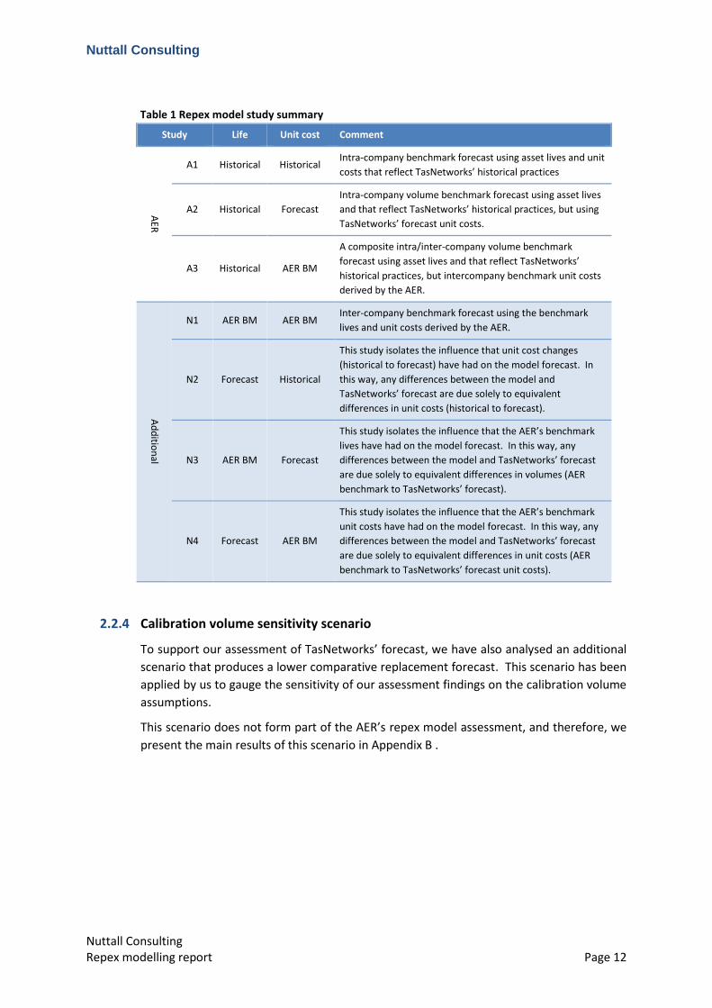
Table 1 Repex model study summary
Study Life Unit cost Comment
AER
A1 Historical Historical Intra-company benchmark forecast using asset lives and unit
costs that reflect TasNetworks’ historical practices
A2 Historical Forecast
Intra-company volume benchmark forecast using asset lives
and that reflect TasNetworks’ historical practices, but using
TasNetworks’ forecast unit costs.
A3 Historical AER BM
A composite intra/inter-company volume benchmark
forecast using asset lives and that reflect TasNetworks’
historical practices, but intercompany benchmark unit costs
derived by the AER.
Ad
ditio
nal
N1 AER BM AER BM Inter-company benchmark forecast using the benchmark
lives and unit costs derived by the AER.
N2 Forecast Historical
This study isolates the influence that unit cost changes
(historical to forecast) have had on the model forecast. In
this way, any differences between the model and
TasNetworks’ forecast are due solely to equivalent
differences in unit costs (historical to forecast).
N3 AER BM Forecast
This study isolates the influence that the AER’s benchmark
lives have had on the model forecast. In this way, any
differences between the model and TasNetworks’ forecast
are due solely to equivalent differences in volumes (AER
benchmark to TasNetworks’ forecast).
N4 Forecast AER BM
This study isolates the influence that the AER’s benchmark
unit costs have had on the model forecast. In this way, any
differences between the model and TasNetworks’ forecast
are due solely to equivalent differences in unit costs (AER
benchmark to TasNetworks’ forecast unit costs).
2.2.4 Calibration volume sensitivity scenario
To support our assessment of TasNetworks’ forecast, we have also analysed an additional
scenario that produces a lower comparative replacement forecast. This scenario has been
applied by us to gauge the sensitivity of our assessment findings on the calibration volume
assumptions.
This scenario does not form part of the AER’s repex model assessment, and therefore, we
present the main results of this scenario in Appendix B .
Nuttall Consulting
Nuttall Consulting Repex modelling report Page 13
3 Repex forecast assessment
In this section we discuss our assessment of TasNetworks’ forecast, using studies defined in
the previous section. In keeping with the AER’s recent approach, this assessment is focused
on the aggregate repex forecast.
3.1 Repex model results and discussion
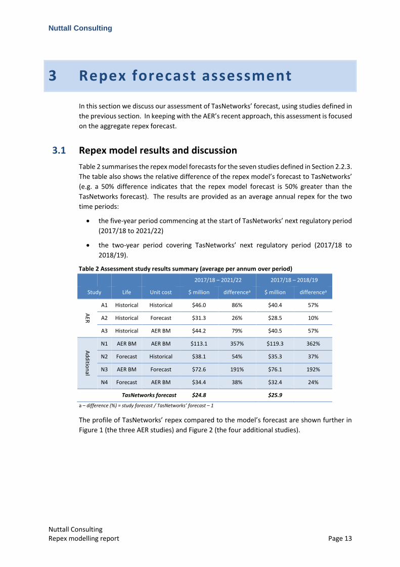
Table 2 summarises the repex model forecasts for the seven studies defined in Section 2.2.3.
The table also shows the relative difference of the repex model’s forecast to TasNetworks’
(e.g. a 50% difference indicates that the repex model forecast is 50% greater than the
TasNetworks forecast). The results are provided as an average annual repex for the two
time periods:
the five-year period commencing at the start of TasNetworks’ next regulatory period
(2017/18 to 2021/22)
the two-year period covering TasNetworks’ next regulatory period (2017/18 to
2018/19).
Table 2 Assessment study results summary (average per annum over period)
2017/18 – 2021/22 2017/18 – 2018/19
Study Life Unit cost $ million differencea $ million differencea
AER
A1 Historical Historical $46.0 86% $40.4 57%
A2 Historical Forecast $31.3 26% $28.5 10%
A3 Historical AER BM $44.2 79% $40.5 57%
Ad
ditio
nal
N1 AER BM AER BM $113.1 357% $119.3 362%
N2 Forecast Historical $38.1 54% $35.3 37%
N3 AER BM Forecast $72.6 191% $76.1 192%
N4 Forecast AER BM $34.4 38% $32.4 24%
TasNetworks forecast $24.8 $25.9
a – difference (%) = study forecast / TasNetworks’ forecast – 1
The profile of TasNetworks’ repex compared to the model’s forecast are shown further in
Figure 1 (the three AER studies) and Figure 2 (the four additional studies).

Nuttall Consulting
Nuttall Consulting Repex modelling report Page 14
Figure 1 Repex model results – AER studies
Figure 2 Repex model results – additional studies
The key points to note from these figures are as follows.
The two charts show that the TasNetworks repex peaked in 2013/14 and TasNetworks is
forecasting this to decline slowly from 2015/16 to 2021/22.
The results of the repex model studies support TasNetworks’ forecast over both time
periods.
All three of the AER assessment studies are forecasting a rising level of repex. For these
three studies, TasNetworks’ forecast is between 54% and 91% of the repex model forecast,
depending on the study and time period.
The three AER studies also indicate that the unit costs used by TasNetworks to prepare its
repex forecast are significantly lower (on average) than its historical unit costs and the AER’s
benchmark unit costs.
$0
$10
$20
$30
$40
$50
$60
2011 2012 2013 2014 2015 2016 2017 2018 2019 2020 2021 2022
rep
lace
me
nt
exp
en
dit
ure
($
mill
ion
s)
NSP historical repex (modelled) NSP historical repex (unmodelled) NSP forecast repex (modelled)
NSP forecast repex (unmodelled) A1 A2
A3
$0
$20
$40
$60
$80
$100
$120
$140
$160
2011 2012 2013 2014 2015 2016 2017 2018 2019 2020 2021 2022
rep
lace
me
nt
exp
en
dit
ure
($
mill
ion
s)
NSP historical repex (modelled) NSP historical repex (unmodelled) NSP forecast repex (modelled)
NSP forecast repex (unmodelled) N1 N2
N3 N4

Nuttall Consulting
Nuttall Consulting Repex modelling report Page 15
The two additional studies, N2 and N4, isolate the effects of the unit cost change,
indicating8:
TasNetworks’ forecast unit costs are 27% to 35% lower than its historical unit costs,
depending on the time period
TasNetworks’ forecast unit costs are 20% to 28% lower than the AER’s benchmark
unit costs , depending on the time period.
The AER studies and additional studies also indicate that the asset lives implicit in
TasNetworks’ repex forecast are significantly longer (on average) than its historical lives and
the AER’s benchmark lives.
The two studies, A2 and N3, isolate the effects of the difference in asset lives, indicating:
TasNetworks’ forecast lives are longer than its historical lives, with a network-level
life of 57 years9 historically compared to 62 years for the forecast.
The AER’s benchmark lives are significantly shorter than TasNetworks’ historical and
forecast lives, with a network-level life of 50 years using the AER benchmark lives.
This very short AER benchmark life compared to the other lives is the reason for the
complete AER intercompany benchmark study, N1, forecasting a significantly greater
level of repex compared to the other studies.
In Appendix C , we discuss in more detail the variations within asset groups.
3.2 Summary and conclusions
Our application of the AER’s assessment method provides very strong support to
TasNetworks’ forecast. TasNetworks’ forecast is significantly below the three AER
assessment studies for both assessment periods.
Furthermore, our studies show that, in aggregate:
the asset lives that underpin TasNetworks’ forecast are significantly longer than its
historical lives and the AER’s intercompany benchmark lives
the asset unit costs that underpin TasNetworks’ forecast are significantly lower than
its historical unit costs and the AER’s intercompany benchmark unit costs.
To provide further support to these findings, we have also examined a more aggressive
replacement scenario (see appendix B ), which produces a lower replacement volume
forecast10. This scenario also produces results that broadly support TasNetworks’ forecast.
On balance, we believe this overall assessment supports TasNetworks’ repex forecast.
8 The percentages quoted reflect the forecast volume-weighted average unit cost. 9 Network-level lives are calculated as the weighted average life, using the asset unit costs. This is the network life
provided on the “age profile summary” sheet of the repex model. 10 This is a lower forecast of the aged replacements that will occur solely due to age/condition type drivers.

Nuttall Consulting
Nuttall Consulting Repex modelling report Page 16
A TasNetworks repex model
development
A.1. The AER’s repex model
A.1.1. Overview of repex model
The AER repex model is an excel workbook, with a structure, formulas and VBA functions
and macros pre-defined in order that it can be used by the AER to develop a network model
of a DNSP and use this to prepare repex forecasts. The model is very similar in principle to
a model used by the UK energy regulator, Ofgem.
The DNSP’s network is constructed within the AER repex model as a series of asset
populations. The model uses a probabilistic replacement algorithm to make predictions of
replacement needs for this population. The probabilistic replacement algorithm assumes
the economic life is normally distributed for any asset population represented within the
model. From this, the model predicts future replacement volumes based upon a current
age profile for the asset population. This approach is similar to survivor-type models, which
are used in various disciplines to model mortality, replacement and reliability.
From an engineering point of view, it is worth noting that although the model relies upon
the ages of assets and uses age-based lives, there is no inherent assumption within the
model (or its use) that purely age-based replacement strategies are used by the DNSP. The
asset life simply reflects the distribution in the life of a population of assets11 - irrespective
of the factors that define the life.
The AER has indicated that it will use this model to make top-down assessments of a DNSP’s
repex forecast, covering both intra-company and inter-company benchmark forecasts.
A.1.2. AER repex model form, inputs and output
Network specification inputs – asset categories, groups and age profiles
As indicated above, a DNSP’s network is defined as a series of distinct asset categories within
the repex model. To facilitate analysis and reporting, each asset category is assigned to a
smaller set of asset groups. In this regard, a model may use 100 asset categories or more,
to improve the accuracy of the analysis, but may use 10 asset groups to provide aggregate
forecast for reporting (and benchmarking) purposes.
An age profile must be provided for each asset category used in the model. This age profile
represents a snap shot of the ages of the population of assets in that category for the initial
11 For example, for many assets, the distribution in the life could result from detailed condition and risk analysis to
determine the optimal time to proactively replace each asset. For others, it could be simply the age when each asset fails.
Nuttall Consulting
Nuttall Consulting Repex modelling report Page 17
year of the model. That is, the age profile is essentially a vector that holds the volume of
assets at one-year increments of age.
The AER has predefined the asset categories and asset groups that the DNSP should use as
the basis of their models. This will be discussed further in A.2.1.
Planning parameters inputs
The model uses three planning parameters to define the approach it uses to predict future
replacement needs:
The replacement life, which is represented as a normal probability distribution is
defined by two parameters: its mean life and the standard deviation of the life.
It is worth noting that the replacement life actually represents the life that an asset
is replaced or the life when a life extension may be used, if this is a feasible option.
These parameters, via the asset age profile, allow the model to predict the future
volume of assets that will need to be replaced (or have their life extended).
The third parameter reflects the average replacement unit cost.
That is, the volume forecast multiplied by the replacement unit cost produces the
expenditure forecast.
Importantly, depending on the asset, the replacement cost parameter may represent
an actual replacement cost, or a life extension cost, or in some cases a blended cost
that represents both.
Model outputs
The model produces various outputs. These outputs provide various measures of the input
age profiles, such as average age, average life, total quantity, and total replacement cost
(i.e. quantity x replacement unit cost).
The model also produces forecasts (by year over a 20-year period), including replacement
volumes, replacement expenditure, average age, and average remaining life.
These various outputs are provided at the asset category, asset group and total network
level. When averages are calculated at the asset group or network level, the model uses a
weighted average using the replacement cost of each asset category as the weighting.
A.1.3. Model planning parameter calibration
The calibration of a DNSP’s model is the critical process that is applied to produce the intra-
company benchmark model.
The calibration process concerns deriving the set of planning parameters that reflects
historical replacement outcomes (volumes and expenditure) over the calibration period
(e.g. the last 5 years)12.
12 It worth noting that a similar process could be applied to calibrate the model to other outcomes, for example the
forecast replacement volumes and expenditure.

Nuttall Consulting
Nuttall Consulting Repex modelling report Page 18
Assuming the actual volumes and expenditure data is available for each asset category in
the model (or a reasonable estimate) then the following process can be used (this process
should be in line with the explanation provided in the AER repex model handbook).
Replacement unit cost
The replacement unit cost parameter for each asset category is simply the actual
expenditure over the calibration period divided by the actual replacement volume over that
period.
Life planning parameters
The two life parameters for each asset category need to be set to ensure the model reflects
the volume replaced over the calibration period.
However, the calculation of the two life planning parameters is more complicated because:
we have two parameters to determine and typically only one variable (the total
volume replaced)
the replacement volume calculated by the model is dependent on the probabilistic
replacement algorithm, and therefore, we need to perform a simulation through
the model
the available age profile represents the end point of the calibration period – not the
start or mid-point.
Therefore, the calibration of the life parameters is slightly more involved and involves the
following two assumptions.
First, in the absence of better information, the need to determine the standard
deviation is removed by making it dependent on the mean. The AER has advised that
it will assume that the standard deviation is taken to be the square root of the mean.
We have used this assumption here.
Second, the mean life is set to ensure that the first year of the forecast produced by
the model equals an adjusted average annual replacement volumes during the
calibration period. The adjustment is set to reflect the initial growth rate in
replacement volumes that is forecast by the model. This adjustment is necessary to
approximate the change due to using the end-point age profile, rather than the
profile that reflects the mid-point of the calibration period13.
Given the above, and allowing for the 5-year calibration period, the adjusted average
annual replacement volumes is calculated as:
(1 + x%)^3.(total volume replaced of asset replaced over calibration period) / 5
where x% is the initial forecast growth rate calculated through the model, and the
power of 3 is necessary to advance the growth over 3 years i.e. from the mid-point in
the calibration period (2011) to the first year of the forecast (2014).
13 It is worth noting that the actual trend in the historical replacement volumes is typically not used as this may be
influenced by incentives associated with the regulatory regime.
Nuttall Consulting
Nuttall Consulting Repex modelling report Page 19
A.2. TasNetworks repex model
A.2.1. TasNetworks repex model structure set up
Setting up the model structure concerns defining the asset categories and asset groups, and
populating the TasNetworks model with the relevant age profiles.
Repex model asset categories and age profiles
The TasNetworks network is constructed within the repex model using the asset
classifications and TasNetworks’ asset age profiles defined in table 5.2.1 of the category
analysis RIN. That is, each asset category in the TasNetworks repex model corresponds to a
line item in table 5.2.1 (i.e. the individual asset categories defined by the AER).
For models used here, TasNetworks has provided a set of age profiles in this format that
represent its network in 2014/15.
Repex model asset groups
The asset groups in the model have been defined using the asset groups specified by the
AER in table 5.2.1 of the category analysis RIN.
A.2.2. Model calibration set up
The calibration of model lives and unit costs is an important element of this modelling
exercise. Therefore, for transparency, we explain our method to do this here.
The model calibration set up involves developing the historical data necessary to perform
the calibration process (discussed in Section A.1.3). This involves calculating for each asset
category in the model (i.e. in table 5.2.1), for the calibration periods (2011 to 2015):
historical repex
historical replacement volumes.
The basis of this data, is the historical replacement volumes and expenditure that
TasNetworks has reported in table 2.2.1 of the category analysis RIN. This data covers the
period from 2010/11 to 2014/15 and across categories that are largely equivalent to table
5.2.1.
This data set has been prepared by mapping and consolidating the asset categories and data
provided in three category analysis RIN templates, which separately covered the following
three time periods14:
2008 to 2013
2013/14
2014/15.
The key steps in preparing the table 2.2.1 data set for the calibration process are as follows:
14 See mapping and consolidation of data in workbook,

Nuttall Consulting
Nuttall Consulting Repex modelling report Page 20
1 Escalation - the table 2.2.1 expenditure has been escalated using CPI data (provided
by TasNetworks) to place all expenditure on a real 2017 basis.
2 2.2.1 to 5.2.1 mapping - rules have been developed that map the 2.2.1 asset
categories (i.e. the asset that was installed) to the 5.2.1 asset categories (i.e. the asset
that was retired). In most cases this was considered to be a direct one-to-one
mapping using the equivalent asset categories in 2.2.1 and 5.2.1. However, in some
circumstances, categories do not map directly or map to multiple categories. In these
case, TasNetworks advised the mapping rules.
Of most note here is wood poles, where mapping is required to allocate the staking
of poles to correct “unstaked” wood pole categories, and the portion the replaced
wood poles to the correct “staked” and “unstaked” wood pole categories.
TasNetworks has provided historical information for these purposes. The
calculations for this can be seen in the model files.
A.2.3. Adjustments to data and calibration
We have applied various adjustment to the TasNetworks data to apply the model and
perform the calibration. The main adjustments are as follows:
For historical overhead conductor expenditure reported in Table 2.2.1 of the RIN,
TasNetworks advised during workshops that this had not been allocated correctly
between the asset categories in this asset group, leading to inappropriate asset
category unit cost for our assessment. Therefore, we reallocated this expenditure,
using the reported volumes and the proportional costs differences as given by the
AER benchmark unit costs.
Because of some non-like-for-like replacements in the transformer asset group, we
linked a number of the transformer asset categories together to calibrate a single
asset life for these linked categories.
A.2.4. Model calibration process
For each asset category in the TasNetworks model, the calibration process has involved the
following steps:
1 Calculate the replacement unit cost as the total historical escalated repex divided by
the total historical replacement volumes (using the mapping described above)15.
2 Determine the mean life that sets the 1st year of the forecast equal to the
(unadjusted) average annual historical volume. Excel’s goal seek function is used for
this purpose.
3 Determine the initial growth rate in the volumes predicted by the model i.e. the
growth from the first to the second year of the forecast.
15 If mapping data results in no historical replacement volumes, for an asset with an age profile, we have applied a
“dummy” unit cost of 0.001. This “dummy” unit costs is necessary to stop the model producing errors, but should not have a material effect on the forecast.

Nuttall Consulting
Nuttall Consulting Repex modelling report Page 21
4 Calculate the adjusted average annual historical volume using this growth rate and
the formula above.
5 Determine the mean life parameter that sets the 1st year of the forecast equal to the
adjusted average annual historical volume. Excel’s goal seek function is used for this
purpose.
Note on replacement volumes
For Scenario 2 discussed in this report, we have added to the replacement volumes provided
in the table 2.2.1 of the RIN with others advised by TasNetworks. The same calibration
process, as described above, has been applied when we have used these amended volumes.
A.2.5. Alterations to the published AER model
We have not changed the underlying structure, format, and predictive algorithms of the AER
repex model. However, we have added a number of sheets to aid in the modelling and
reporting exercise.
These main additional sheets are:
Three sheets have been added to contain the TasNetworks input data, covering:
- RIN table 2.2.1
- RIN table 5.2.1
- TasNetworks forecast.
Three sheets have been added to facilitate the mapping between tables 5.2.1 and
2.2.1, and the calibration process. These sheets are:
- Asset map
- Volume map16
- Forecast map17
- Other data.
A sheet has been added to aid in the reporting of results and to produce comparisons
with the TasNetworks forecast:
- Comparison Ch.
16 The assumptions that map table 5.2.1 to table 2.2.1 containing TasNetworks’ historical repex and replacement volumes
are provided on the Volume map sheet. 17 The assumptions that map table 5.2.1 to table 2.2.1 containing TasNetworks’ forecast repex and replacement volumes
are provided on the Forecast map sheet.

Nuttall Consulting
Nuttall Consulting Repex modelling report Page 22
B Calibration volume sensitivity
scenario
B.1. Considerations for scenario
Although the model results using the AER assessment method provide significant support
to TasNetworks forecast (see Section 3), we have some concerns with the appropriateness
of the method, given the extent that it produces a forecast above TasNetworks’. Of most
note here is the future growth rate in repex, forecast by the three AER studies, which is
particularly high for the overhead conductor and transformer asset groups.
These high growth rates can occur when the asset life is long compared to the age profile,
and so, the model considers that the asset population is in a very early stage of its
replacement cycle. Long lives are generated when the replacement volume is low relative
to the asset population.
To examine this further, we examined the recent asset age profile in the model (i.e. assets
installed over the historical calibration period). The age profile indicates that, for the asset
groups showing the most significant repex growth, a significantly higher number of assets
have been installed over the calibration period than are reported to have been replaced in
Table 2.2.1 of the RIN.
This is not necessarily a problem in most circumstances as other drivers can commonly
cause the need for these new assets (e.g. new network developments). However,
TasNetworks considered that this was unlikely to be the case in its circumstances as there
had been little new network development over this period. The view was that a material
portion of aged assets were being replaced through activities, such as network
augmentation and customer connection activity. As such, these asset replacements where
not reported in Table 2.2.1 of the RIN. Consequently, the volumes used for the historical
calibration was understating the true volumes, and therefore, the calibrated life would be
too long.
This sensitivity scenario was applied to investigate these concerns.
B.2. Scenario calibration volume assumptions
This scenario represents a variation to the calibration method the AER has applied.
This variation involves using additional replacement volumes added to the volumes
TasNetworks has reported in its RIN. As noted above, these additional volumes reflect the
replacement of aged assets that will have occurred for other reasons (e.g. augmentation
and connections), and so would not have been reported in the repex tables of the RIN.
Nuttall Consulting
Nuttall Consulting Repex modelling report Page 23
This variation results in shorter calibrated lives – as these lives need to reflect a higher
volume of replacements. Therefore, the model, itself, is forecasting a higher volume of
replacements because of these shorter lives. However, this scenario assumes that a similar
proportion of these forecast replacements will occur through other drivers (e.g. network
augmentation and connections) as occurred historically. This assumption typically reduces
the volume of replacements, forecast by the model, that would be allocated to the repex
expenditure category, and so, results in a more aggressive (i.e. lower) comparative forecast.
The results presented in this appendix, only cover the proportion that are assumed to be
replaced due solely to age/condition considerations.
It is important to note that due to the time constraints of this project, TasNetworks has not
provided an accurate estimate of these additional volumes18. Therefore, the following
assumptions have been applied19:
Poles – no additions, assuming all reported in RIN
Overhead conductors – 80% of assets installed over last five years (as indicated by
age profile) replaced aged assets
Underground conductors – additional 2 km per annum replaced aged assets
Services – no additions, assuming all reported in RIN
Transformers - 80% of assets installed over last five years (as indicated by age profile)
replaced aged assets
Switchgear - 80% of assets installed over last five years (as indicated by age profile)
replaced aged assets.
B.3. Scenario model results and discussion
Table 3, Figure 3 and Figure 4 show the equivalent study results for this scenario, as
discussed in Section 3.1.
As expected, the various studies in this scenario forecast a lower level of repex.
Nonetheless, this scenario still provides results that support TasNetworks’ forecast. All
three of the AER studies still forecast a rising level of repex, with TasNetworks’ forecast
between 67% and 95% of the repex model’s forecast, over the five-year assessment time
period.
The AER studies and additional studies also still indicate that the asset lives implicit in
TasNetworks repex forecast are longer (on average) than its historical lives and the AER’s
benchmark lives.
The two studies, A2 and N3, isolate the effects of the difference in asset lives, indicating:
18 Providing accurate estimates would have required detailed analysis of past projects by TasNetworks. This additional
effort is not justified given this scenario is not being used for the primary assessment of TasNetworks’ forecast. 19 Note, where the additional volume has been calculated from the age profile the adjustment has only been applied to
assets where this would be material on the forecast.

Nuttall Consulting
Nuttall Consulting Repex modelling report Page 24
TasNetworks’ forecast lives are longer than its historical lives, with a network-level
life of 54 years historically compared to 57 years for the forecast.
The network-level life of 50 years, derived using the AER’s benchmark lives, is still
significantly shorter than TasNetworks’ historical and forecast lives.
This scenario only affects asset lives, and therefore, the forecast unit cost findings discussed
in the main body of this report still apply to this scenario.
Comment on results for two-year regulatory period
TasNetworks’ forecast is 5% above the repex model study over the two-year regulatory
period. This under-forecast by the model only occurs in the study using historical lives and
forecast unit costs. This result suggests replacement volumes may be too high over this
period, compared to TasNetworks’ history.
However, as discussed in Section 2.2.1, we believe this period is likely to be too short for a
reliable assessment through the repex model. Furthermore, we consider that the additional
volume assumptions noted above are fairly aggressive. Therefore, this 5% variance in the
context of all the other much more positive variances should be treated with some caution
with regard to it being the basis for rejecting TasNetworks’ forecast.
As such, if the significance of this result remained a concern then it would need to be
investigated further using other assessment techniques that the AER may apply to consider
the appropriateness of TasNetworks’ forecast annual repex profile.
Table 3 Scenario study results summary (average per annum over period)
2017/18 – 2021/22 2017/18 – 2018/19
Study Life Unit cost $ million differencea $ million differencea A
ER
A1 Historical Historical $36.8 49% $34.1 32%
A2 Historical Forecast $26.2 5% $24.8 -5%
A3 Historical AER BM $36.7 48% $35.0 36%
Ad
ditio
nal
N1 AER BM AER BM $67.6 173% $74.0 187%
N2 Forecast Historical $38.1 54% $36.1 40%
N3 AER BM Forecast $46.1 85% $49.0 88%
N4 Forecast AER BM $34.4 38% $33.1 27%
TasNetworks forecast $24.8 $25.9
a – difference (%) = study forecast / TasNetworks’ forecast – 1

Nuttall Consulting
Nuttall Consulting Repex modelling report Page 25
Figure 3 Scenario repex model results – AER studies
Figure 4 Scenario repex model results – additional studies
$0
$5
$10
$15
$20
$25
$30
$35
$40
$45
2011 2012 2013 2014 2015 2016 2017 2018 2019 2020 2021 2022
rep
lace
me
nt
exp
en
dit
ure
($
mill
ion
s)
NSP historical repex (modelled) NSP historical repex (unmodelled) NSP forecast repex (modelled)
NSP forecast repex (unmodelled) A1 A2
A3
$0
$10
$20
$30
$40
$50
$60
$70
$80
$90
$100
2011 2012 2013 2014 2015 2016 2017 2018 2019 2020 2021 2022
rep
lace
me
nt
exp
en
dit
ure
($
mill
ion
s)
NSP historical repex (modelled) NSP historical repex (unmodelled) NSP forecast repex (modelled)
NSP forecast repex (unmodelled) N1 N2
N3 N4

Nuttall Consulting
Nuttall Consulting Repex modelling report Page 26
C Assessing forecast differences
In Section 3, we used the TasNetworks repex model to provide a reasonable bound for
TasNetworks’ repex forecast, using an approach the AER has applied recently.
In this appendix, we use the TasNetworks repex model to identify the asset groups that vary
the most between the model and TasNetworks’ forecast, and in turn, to determine how the
model’s lives and unit costs contribute to this variance.
These findings indicate the asset matters that the AER may have the most concern with
should it use the repex model for these purposes.
C.1. Overview of assessment approach
The repex variances between the model and TasNetworks’ forecast can be due to
differences in the forecast replacement volumes (which relate to differences in the
underlying lives) or differences in the unit costs, or more typically a combination of the two.
To distinguish between these two factors, and be able to gauge the contributions on a
similar monetary scale (noting here that the repex associated with different volumes in the
model can vary by orders of magnitude), we have used a similar approach to that used at
the network level in the previous section.
This approach has used the results from a subset of the studies to assess life and unit costs
on an intra-company basis (i.e. relative to history and a business-as-usual approach) and an
inter-company basis (i.e. relative to the AER benchmark lives and unit costs).
We have used these studies to determine which asset groups show the greatest variance in
repex. We have then used this to identify which asset category lives or unit costs are causing
this difference.
C.2. Results of assessment
Table 4 Summary of asset group comparison results (study variance to TasNetworks’ forecast)
Intra-company studies Inter-company studies
study: A1 A2 N2 N1 N3 N4 TasNetworks
Life: Historical Historical Forecast AERBM AERBM Forecast forecast
Unit cost: Historical Forecast Historical Forecast Forecast AERBM $ millions
Poles 45% 29% 9% 329% 138% 62% $7.4
OH conductors 381% 79% 158% 401% 418% 17% $2.7
UG cables 0% 20% -34% 31% 30% -25% $2.3
Services -31% -42% -2% 109% 5% 61% $2.9
Transformers 76% -43% 325% -31% 18% -22% $3.7
Switchgear -59% -9% -47% 87% -33% 71% $5.8
Total 49% 5% 54% 173% 85% 38% $24.7

Nuttall Consulting
Nuttall Consulting Repex modelling report Page 27
The results of these studies are presented above. The red shading indicates where the
model’s repex forecast is more than 10% below TasNetworks’. The green shading indicates
where the model’s repex forecast is more than 10% above TasNetworks’.
The results of the intra-company comparison (i.e. study A1 – TasNetworks’ forecast relative
to the forecast using TasNetworks’ historical lives and unit costs) indicate the following:
The services and switchgear asset groups show the greatest under-forecast by the
model compared to TasNetworks’ forecast.
Conversely, the poles, overhead conductors, and transformer asset groups show a
significant over-forecast.
The underground cable group show a very close match between the model and
TasNetworks’ forecast.
Differences between the historical lives and unit costs and those underpinning
TasNetworks’ forecast tend to contribute in opposing ways to form the repex
difference.
The results of the inter-company comparison studies (i.e. study N1 – TasNetworks’ forecast
relative to a forecast using AER’s benchmark lives and unit costs) indicate the following:
TasNetworks’ forecast for all the asset groups, other than transformers, is
significantly below the repex model’s forecast using the AER’s benchmark lives and
unit costs.
The effects of the shorter lives in the AER benchmarks is most pronounced for the
poles and overhead conductor categories. Switchgear is the only asset group where
the AER benchmark lives are longer than TasNetworks’ forecast lives.
TasNetworks’ forecast unit costs are significantly lower than the AER benchmarks in
all asset groups other than underground cables and transformers, where they are
noticeably higher.
We discuss each asset group in more detail below.
Note on life and unit cost terminology in discussion below
When discussing differences in asset group lives and unit costs, the asset group life or unit
cost implied by the discussion is a weighted average life across the relevant asset categories
calculated through the model. The weightings applied to unit costs are the forecast volumes
and the weightings applied to volumes are the forecast unit costs.
C.2.1. Poles
TasNetworks’ forecast for the poles asset group is lower than the intra-company and the
inter-company studies.
With regard to volume and life differences:

Nuttall Consulting
Nuttall Consulting Repex modelling report Page 28
TasNetworks’ forecast calibrated lives are longer than its historical lives. The asset
categories of most note here are staked and unstaked HV wood poles, which have
noticeably longer lives for TasNetworks’ forecast (5 to 10 years longer).
TasNetworks’ forecast calibrated lives are much longer than the AER’s benchmark
lives. The asset categories of most note here are unstaked HV wood poles, which
have much shorter lives for the AER benchmarks (14 to 17 years shorter).
With regard to unit cost differences:
TasNetworks’ forecast unit costs are lower than its historical unit costs. At the asset
category level, staked pole replacement unit costs have increased (23%), but this is
offset by a reduction in the unit costs for unstaked poles (i.e. 13% reduction in the
blended staking and replacement cost).
TasNetworks’ forecast unit costs are lower than the AER’s benchmark unit costs. The
asset categories of most note here are unstaked HV wood poles, where the AER
benchmark unit costs are approximately 75% greater than the TasNetworks forecast
unit costs.
The above indicates that the effect of the lower unit costs and longer lives in TasNetworks’
forecast combine to produce the overall positive finding for TasNetworks’ pole forecast.
C.2.2. Overhead conductors
TasNetworks’ forecast for the overhead conductor asset group is significantly lower than
the intra-company and the inter-company studies.
With regard to volume and life differences:
TasNetworks’ forecast calibrated lives are longer than its historical lives, in the order
of 5 to 6 years.
TasNetworks’ forecast calibrated lives are much longer than the AER’s benchmark
lives, in the order of 15 to 20 years.
With regard to unit cost differences:
TasNetworks’ forecast unit costs are significantly lower than its historical unit costs,
where all categories show a noticeably lower unit cost (40% to 70% reduction).
TasNetworks’ forecast unit costs are lower than the AER’s benchmark unit costs,
where all asset categories (other than SWER) are 12% to 33% lower.
The above indicates that the effect of the lower unit costs and longer lives combine to
produce the overall very positive results for TasNetworks’ overhead conductor forecast.
C.2.3. Underground cables
TasNetworks’ forecast for the underground cable asset group is very similar to the intra-
company study, but is lower than the inter-company study.
With regard to volume and life differences:

Nuttall Consulting
Nuttall Consulting Repex modelling report Page 29
TasNetworks’ forecast calibrated lives are longer than its historical lives and the AER
benchmarks. The most significant asset category is LV cable, which has a slightly
longer life compared to its historical life or the AER benchmark, in the order of 2
years.
With regard to unit cost differences:
TasNetworks’ forecast LV cable unit cost is higher than its historical unit cost and the
AER benchmark, indicating an approximately 80% increase over both of these unit
costs.
The above indicates that the effect of the longer lives but higher unit costs counteract each
other to produce the over positive finding.
C.2.4. Services
TasNetworks’ forecast for the services asset group is higher than the intra-company study,
but much lower than the inter-company study.
With regard to volume and life differences:
TasNetworks’ forecast calibrated lives are shorter than its historical calibrated lives,
where the life of simple residential services is much shorter for TasNetworks’ forecast
(45 years compared to 54 years historically).
TasNetworks’ forecast calibrated lives is however very slightly longer than the AER
benchmark, which is 44 years.
With regard to unit cost differences:
TasNetworks’ forecast calibrated unit costs are very similar to its historical unit costs,
but these are approximately 40% lower than the AER benchmark unit cost.
The above indicates that the effect of the shorter service life is the cause of the
TasNetworks’ higher forecast compared to the intra-company study, but the lower unit cost
is the reason for the lower forecast compared to the intercompany study.
C.2.5. Transformers
TasNetworks’ forecast for the transformer asset group is lower than the intra-company
benchmark study, but it is the only asset group where TasNetworks’ forecast is higher than
the intercompany benchmark study.
With regard to volume and life differences:
TasNetworks’ forecast calibrated lives are shorter than its historical calibrated lives.
The asset categories with significantly shorter lives are “Kiosk Mounted ; < = 22kV ; >
600 kVA ; Multiple Phase” (36 years shorter), “Ground Outdoor / Indoor Chamber
Mounted; ˂ 22 kV ; > 60 kVA and < = 600 kVA ; Multiple Phase” (17 years shorter)
and “Ground Outdoor / Indoor Chamber Mounted; ˂ 22 kV ; > 600 kVA ; Multiple
Phase” (5 years shorter).

Nuttall Consulting
Nuttall Consulting Repex modelling report Page 30
TasNetworks’ forecast calibrated lives are longer than the AER’s benchmark lives.
Although, at the asset category level, some lives are longer and others are shorter
than the AER benchmarks (ranging between 13 years longer and 5 years shorter than
the AER benchmarks).
With regard to unit cost differences:
TasNetworks’ forecast calibrated unit costs are significantly lower than its historical
unit costs. However, there are some anomalous results that suggest caution may
need to be applied on making any inferences from these findings.
“Kiosk Mounted ; < = 22kV ; > 60 kVA and < = 600 kVA ; Multiple Phase” had a
historical unit cost of $8,000, which seems unrealistically low. Conversely, “Ground
Outdoor / Indoor Chamber Mounted; ˂ 22 kV ; > 60 kVA and < = 600 kVA ; Multiple
Phase” and “Ground Outdoor / Indoor Chamber Mounted; ˂ 22 kV ; > 600 kVA ;
Multiple Phase” had historical unit cost of over $700,000, which seems unrealistically
high. All three asset categories have forecast unit costs in the order of $60,000, which
seems more reasonable.
TasNetworks’ forecast calibrated unit costs are higher than the AER’s benchmark unit
costs. The lower unit costs of the AER benchmarks seems to be fairly consistent
across the transformer asset categories used by TasNetworks.
C.2.6. Switchgear
TasNetworks’ forecast for the switchgear asset group is significantly higher than the intra-
company study, but significantly lower than the inter-company study.
With regard to volume and life differences:
TasNetworks’ forecast calibrated lives are broadly similar to its historical lives, with
the result showing TasNetworks’ forecast lives marginally shorter. This result is
driven by the two circuit breaker categories, which appear to have anomalously low
forecast lives (12 years for 11 kV breakers and 23 years for 22 kV breakers). The
forecast lives for the other asset categories are higher than the historical lives.
TasNetworks’ forecast calibrated lives are shorter than the AER’s benchmark lives.
However, this result is driven by the same anomalous circuit breaker lives discussed
above. The forecast lives of the other categories are longer than the AER
benchmarks.
With regard to unit cost differences:
TasNetworks’ forecast calibrated unit costs are higher than its historical unit costs.
This result however seems to be driven by anomalous unit costs across all categories.
Most notably, the “<=11 kV fuse” category historically had a unit costs of $19 per unit,
but this has increased to $2000 per unit. Similarly, 22 kV switch costs have nearly
tripled.
There could be various reasons for these large changes. It could simply be an error
in the reporting in the RIN tables. However, this could suggest that there has been a

Nuttall Consulting
Nuttall Consulting Repex modelling report Page 31
change in the asset activity from history to forecast; for example, the replacements
of fuses changing to the replacement of fuse assemblies.
TasNetworks’ forecast calibrated unit costs are much lower than the AER’s
benchmark unit costs. This is most notable for the >=11 kV circuit breakers, where
the AER benchmark is more than double TasNetworks forecast unit cost.
Given the concerns noted above, care is need in drawing too much from the findings for this
asset group category. TasNetworks may need to review its own data first to ensure there is
consistency between how it has reported historical and forecast repex and replacement
volumes, and that these volumes are reported on a consistent basis to the relevant age
profile.
C.3. Summary and conclusions
Our assessment at the asset level has found a number of instances where TasNetworks’
forecast asset lives are longer than its historical lives or the AER’s benchmark lives, and
TasNetworks’ forecast unit costs are higher than its historical unit costs or the AER’s
benchmark unit costs. These findings could suggest areas that the AER may investigate
should it have concerns with TasNetworks’ repex forecast.
The most significant variances of this type are as follows:
Services, transformer and switchgear asset groups all have some significant asset
categories where the forecast asset lives are significantly shorter than TasNetworks’
historical lives. Furthermore, the forecast lives for the circuit breakers categories in
the switchgear group are significantly shorter than the AER’s benchmark lives.
Underground cables and switchgear asset groups have some significant asset
categories where the forecast asset unit costs are significantly higher than
TasNetworks’ historical unit costs. Furthermore, the underground cables and
transformer asset groups have forecast asset unit costs that are significantly higher
than the AER’s benchmark unit costs.
With regard to the transformer and switchgear variances, some of these appear so great
that they could be anomalous. Therefore, TasNetworks may need to investigate its RIN
reporting of the volumes and expenditure (i.e. Table 2.2.1) in these asset groups to confirm
data has been allocated correctly.