AEA Jan paper - utdallas.edumurdoch/NeighborhoodChange/LIHTC/Di_Murdoch.… ·...

The Impact of LIHTC Program on Local Schools

PRELIMINARY PAPER FOR 2010 ASSA CONFERENCE PLEASE DO NOT QUOTE OR CITE WITHOUT OUR PERMISSION

Wenhua Di

Federal Reserve Bank of Dallas

James C. Murdoch University of Texas at Dallas

January 2010

Abstract

The Low Income Housing Tax Credit (LIHTC) program has produced rental homes for low-‐income residents for over two decades. Using the administrative data on LIHTC projects and elementary schools in the state of Texas, we find that the overall impact of LIHTC projects on nearby schools is essentially zero. That the perception of possible deterioration in school performance becomes the key reason for “nimbyism” against LIHTC, our study suggests these fears are unfounded. The study uses a panel of school-‐level performance data for the entire state of Texas. The school-‐level data is geographically associated with LIHTC projects, facilitating a panel-‐type estimation of the consequences of the LIHTC program on school-‐level academic ratings. Disclaimer The views expressed in the paper are those of the authors and do not necessarily represent the views of the Federal Reserve Bank of Dallas or the Federal Reserve System.

Introduction

The availability of affordable housing is a pressing issue in most metropolitan areas in

the United States. Many communities struggle to provide housing options for low-‐ and

moderate-‐income residents. In high cost metropolitan areas, housing options for professionals

such as teachers and police officers are often scarce in the communities where they work. Even

more challenging is housing very low-‐income residents, such as families living off minimum

wage salaries. In response to these shortages, several public policies and programs have been

tried, including public housing, housing vouchers and certificates, inclusionary zoning, tax

preferences for low-‐income housing, and local affordable housing mandates or offsets.

Finding a suitable location for low-‐income housing is a challenge for both developers

and municipal officials. Local residents often exhibit a “not in my backyard” (NIMBY) attitude.

Community opposition may stem from building designs or quality, the potential impacts to

historical neighborhood characters, the decline in open space, perceptions of decreases in

public services, fear of enhanced criminal activity, and perceptions of negative effects on

property values (Downs 1982; Finkel, Climaco et al. 1996; Pendall 1999; Turner, Popkin et al.

2000; Nguyen 2005). Moreover, parents in the potentially impacted neighborhoods may be

concerned that their neighborhood public schools will become over crowed and that low-‐

income kids from publicly-‐driven multi-‐family housing will exert negative peer influences. Such

NIMBY sentiments may deter the construction of new low-‐income housing from certain

neighborhoods or drive residents to “flee” the neighborhood (or local school) after the

construction of the low-‐income units, causing a downward spiral in the local schools.

Several studies have used changes in property values to estimate the potential impacts

of publicly-‐driven low-‐income housing on neighborhoods. Recent reviews can be found in

Nguyen and in Ezzet-‐Lofstrom and Murdoch (Nguyen 2005; Ezzet-‐Lofstrom and Murdoch 2007).

However, we are not aware of any studies that have looked at the direct relationship between

the emergence of low-‐income housing and the academic performance of nearby schools. Thus,

the purpose of this paper is to investigate whether low-‐income housing, built through the Low

Income Housing Tax Credit program, affects neighborhood public school performance. To carry

out this purpose, we created a panel data set on approximately 4000 elementary schools in

Texas by spatially merging data from the almost 2000 Low-‐Income Housing Tax Credit (LIHTC)

program properties in Texas with Texas Education Agency accountability data on the

elementary schools. The data set facilitates estimates of the relationship between changes in

school academic rating and changes the number of nearby LIHTC units. Generally, we find little

evidence to suggest negative effects from LOIHTC units. In fact, the contemporaneous impacts

appear to be positive, significant and robust to alternative specifications. Of setting these, the

one period lag effects are negative and have almost the same magnitiude.

The remainder of the paper is organized as follows. First, we provide an overview of the

LIHTC program with a focus on the state of Texas. Then, we discuss some of the ways that

potential LIHTC units could impact local schools. In the fourth section, we describe the data and

main variables. The fifth section contains the empirical anlysis followed by some discussion

about the results.

Overview of Low Income Housing Tax Credit Program

The LIHTC program is part of the Tax Reform Act of 1986. It is the largest program for

producing affordable rental housing. Primarily serving residents making 60 percent of area

median income or less, the LIHTC program gives a dollar-‐for-‐dollar federal tax credit to private

investors in return for project equity, reducing the amount of required finance and thereby

making rents more affordable. The typical amount of tax-‐credit equity raised in a 9 percent tax-‐

credit transaction is between 45 percent and 75 percent of the development costs.

Investors such as financial institutions and corporations purchase the tax credits to

lower their federal tax liability over a 10-‐year period. Financial institutions that purchase

credits for developments within their Community Reinvestment Act (CRA) assessment areas get

CRA credit and all investors earn attractive rates of return. The yields on tax credit investments

in recent years have averaged between 5 and 7 percent. Federal law requires that the rents and

incomes remain restricted for 15 years, but Texas employs an extended land-‐use agreement

that retains the units in the affordable housing stock for at least 30 years.

The LIHTC program has produced approximately 2.5 million units nation-‐wide. In Texas

the Department of Housing and Community Affairs (TDHCA) administers the program with

some oversight from the state Legislature. To date, Texas has allocated approximately $750

million in tax credits to developers, leading to an infusion of equity that has contributed to the

development of nearly 200,000 affordable housing units. Competition for the credits has been

fierce among developers. Like most other states, Texas leans heavily on this public–private

partnership, which brings the Internal Revenue Service, the state housing agency, investors and

developers together in pursuit of solutions for low-‐income residents seeking quality, affordable

housing.

The stated goal of Texas’ LIHTC program is to encourage diversity through the broad

geographic allocation of credits, promote maximum use of the available tax credit amount and

allocate credits among as many different developments as possible without compromising

housing quality. LIHTC properties can include new construction and the redevelopment of

underutilized properties. The program in Texas also requires a minimum 15 percent At-‐Risk

Development set-‐aside to allocate to projects with other subsidies that are set to expire.

Figure 1 shows tax credit allocations cross-‐tabulated with the number of units created.

The red line shows a continuous increase in allocations to Texas LIHTC properties since 1989.

The substantial rise in state allocations by Congress in 2001 and the booming production of

bond transactions around the same time augmented the tax credits awarded. The green line

illustrates the number of LIHTC units developed between 1989 and 2007.

Figure 1 LIHTC Units and Program Funding in Texas

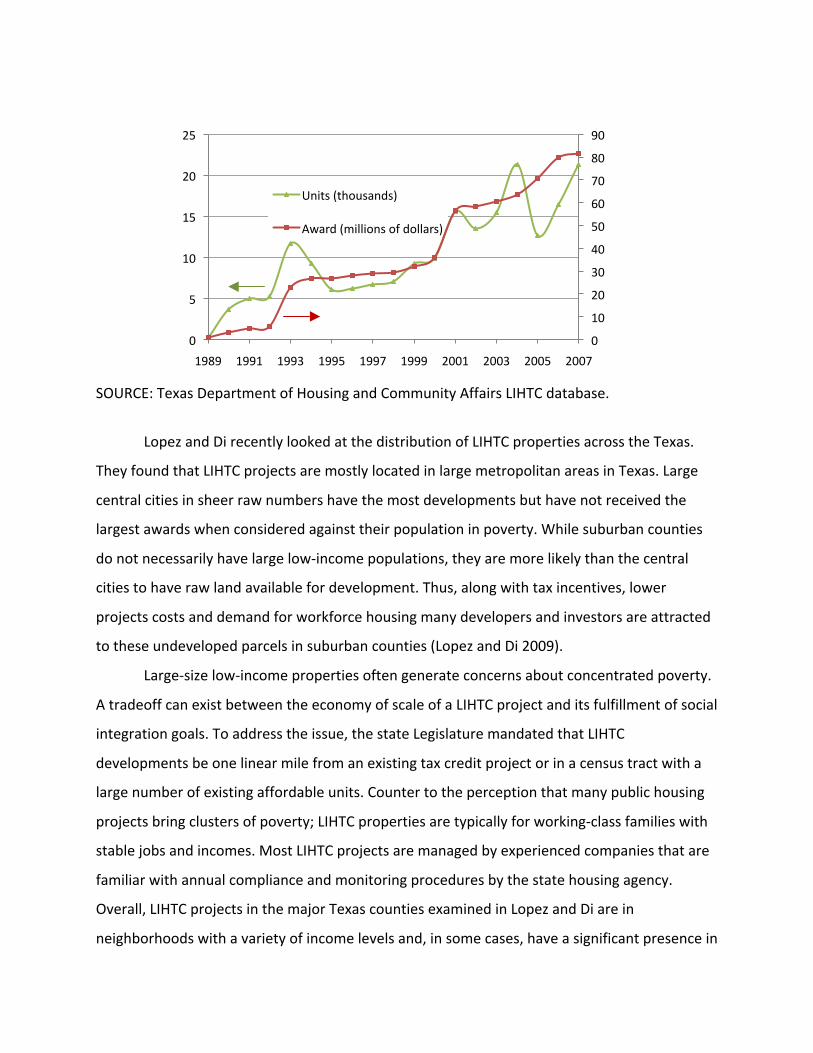
SOURCE: Texas Department of Housing and Community Affairs LIHTC database.

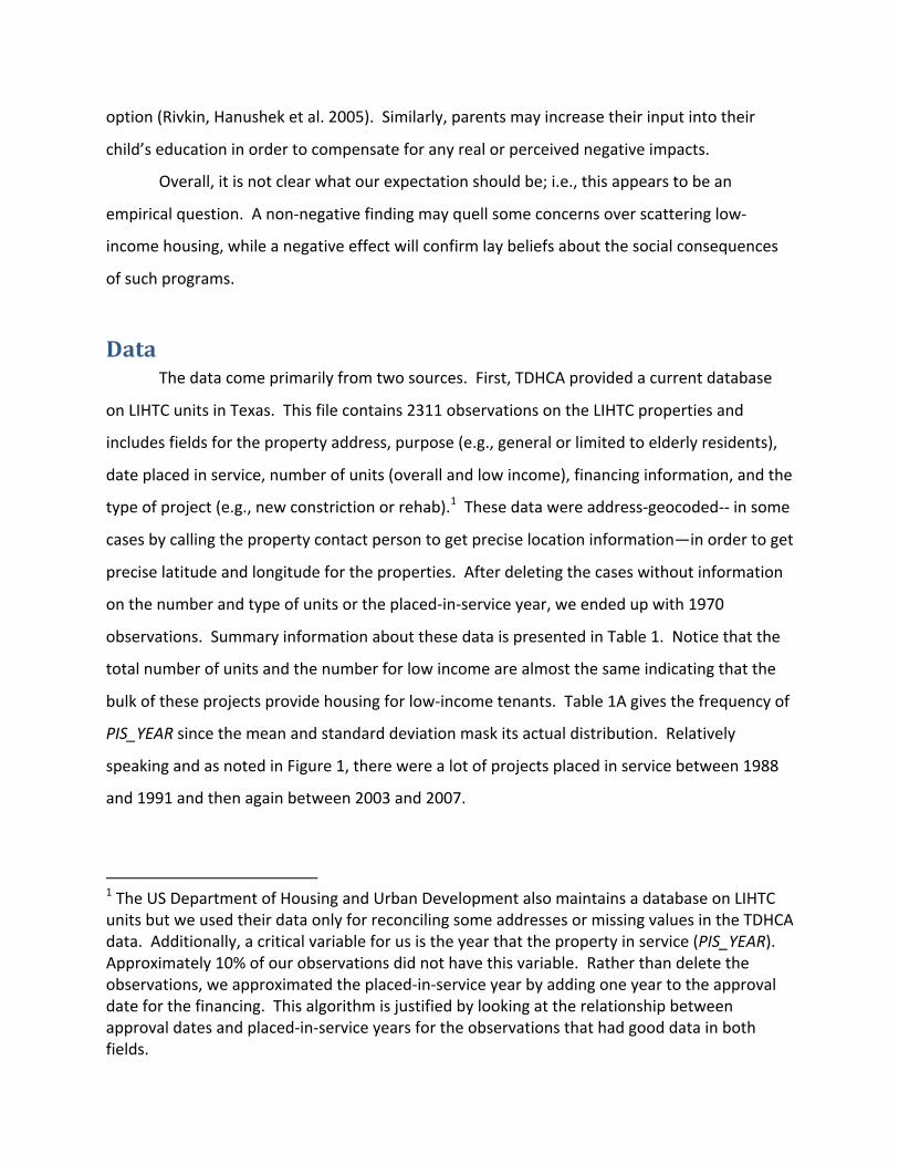
Lopez and Di recently looked at the distribution of LIHTC properties across the Texas.

They found that LIHTC projects are mostly located in large metropolitan areas in Texas. Large

central cities in sheer raw numbers have the most developments but have not received the

largest awards when considered against their population in poverty. While suburban counties

do not necessarily have large low-‐income populations, they are more likely than the central

cities to have raw land available for development. Thus, along with tax incentives, lower

projects costs and demand for workforce housing many developers and investors are attracted

to these undeveloped parcels in suburban counties (Lopez and Di 2009).

Large-‐size low-‐income properties often generate concerns about concentrated poverty.

A tradeoff can exist between the economy of scale of a LIHTC project and its fulfillment of social

integration goals. To address the issue, the state Legislature mandated that LIHTC

developments be one linear mile from an existing tax credit project or in a census tract with a

large number of existing affordable units. Counter to the perception that many public housing

projects bring clusters of poverty; LIHTC properties are typically for working-‐class families with

stable jobs and incomes. Most LIHTC projects are managed by experienced companies that are

familiar with annual compliance and monitoring procedures by the state housing agency.

Overall, LIHTC projects in the major Texas counties examined in Lopez and Di are in

neighborhoods with a variety of income levels and, in some cases, have a significant presence in

0

10

20

30

40

50

60

70

80

90

0

5

10

15

20

25

1989 1991 1993 1995 1997 1999 2001 2003 2005 2007

Units (thousands)

Award (millions of dollars)

middle-‐ and upper-‐income areas. These findings suggest that the Texas LIHTC program may

have contributed to de-‐concentrating poverty and integrating low-‐income households into

higher-‐income neighborhoods.

Potential Effects of the LIHTC Program on Schools There are several ways that the LIHTC policy could impact local schools. In the short run,

LIHTC properties may foster integration of poor minority children into traditionally segregated

white neighborhoods. To the extent that these children come from segregated minority

environments there is some evidence to suggest that their educational performance will be

below the average in their new school (Vigdor and Ludwig 2007; Jacob and Ludwig 2009).

Although there is some evidence to suggest that that movers are no less well adjusted to school

than non-‐movers (Alexander, Entwisle et al. 1996), mobility is also likely a negative factor (Mao,

Whitsett et al. 1997). Therefore, the immediate impact may be to lower the school’s overall

standardized test scores and their rating. On the other hand, families that select into LIHTC

properties may have characteristics that make their children relatively high performers in

school. After all, the family has managed to move into a subsidized development that is most

likely in a better neighborhood than their other opportunities. For example, a survey of a

sample of LIHTC residents found that 23% came from public housing and more than 50% rated

their current housing better than their previous housing, suggesting that LIHTC units provide a

gateway to better private sector housing (Buron, Nolden et al. 2000).

The literature is unsettled as to whether or not we should expect the negative effects to

linger (or even get worse) for several reasons. First, the role of peers in modifying achievement

is at best complicated and this is an active area of research. Cooley finds stronger peers effects

within reference groups (e.g., the same race) perhaps suggesting that importing some lower

performing minority kids into a school will not negatively influence the majority (Cooley 2006).

Hoxby also finds that students are influenced by their peers and that the effect may be stronger

among peers of the same race (Hoxby 2000). Burke and Sass find nonlinear effects due to

peers. For example, a mean preserving spread in achievement may decrease achievement

gains. On the other hand, the lowest achieving students, especially in elementary school, get

sizable benefits from middle and high performing peers (Burke and Sass 2008). Hanushek et al.

also find positive per effects. However, they find that the variance does not matter and that

students throughout the achievement distribution seem to benefit from higher performing

peers (Hanushek, Kain et al. 2003). In contrast, Evans, Oates, et al. find that peer effects

disappear after controlling for simultaneity (Evans, Oates et al. 1992).

There is some evidence that diversity is good. The post-‐ hoc Black-‐White and Hispanic-‐

White achievement gaps appear to be smaller in racially diverse schools (Bali and Alvarez 2004)

and the SAT score differential between blacks and whites is greater in more racially segregated

cities. Moreover, the neighborhood characteristics seem to matter the most not the

segregation within schools (Card and Rothstein 2007).

A second area for uncertainty on what to expect about the longer-‐term impacts of LIHTC

properties on local schools encompasses the behavioral responses of parents, school

administrators and teachers. As noted above, some families may simply move from the LIHTC-‐

impacted area although using real estate data from the Dallas area Ezzet-‐Lofstrom and

Murdoch did not find depreciated property values as a result of proximity to LIHTC units (Ezzet-‐

Lofstrom and Murdoch 2007). Not withstanding, if some of the best achieving students vacate

the local school, the overall rating would suffer. Teachers, now confronted with more minority

students, may also seek alternative locations (Scafidia, Sjoquistb et al. 2007). Moreover, the

pre-‐existing input combinations may be suboptimal after the opening of the LIHTC units. In

particular, with the arrival of poorer performing students, pre-‐existing class sizes may be too

large (Lazear 2001). Another behavioral impact from teachers concerns assessments. Ouazad

finds that teachers give higher assessments to children of their own race. Thus, if the LIHTC

children enter a situation where most of their teachers are different in terms of race and

ethnicity their performance may not improve (Ouazad 2008).

On the other hand, administrators do seem to respond to accountability ratings

(Hanushek and Raymond 2005). An initial negative impact from LIHTC properties may be met

with additional resources and better teachers. Both better teachers and smaller classes could

mitigate any negative impacts although better teachers appear to be the more powerful policy

option (Rivkin, Hanushek et al. 2005). Similarly, parents may increase their input into their

child’s education in order to compensate for any real or perceived negative impacts.

Overall, it is not clear what our expectation should be; i.e., this appears to be an

empirical question. A non-‐negative finding may quell some concerns over scattering low-‐

income housing, while a negative effect will confirm lay beliefs about the social consequences

of such programs.

Data The data come primarily from two sources. First, TDHCA provided a current database

on LIHTC units in Texas. This file contains 2311 observations on the LIHTC properties and

includes fields for the property address, purpose (e.g., general or limited to elderly residents),

date placed in service, number of units (overall and low income), financing information, and the

type of project (e.g., new constriction or rehab).1 These data were address-‐geocoded-‐-‐ in some

cases by calling the property contact person to get precise location information—in order to get

precise latitude and longitude for the properties. After deleting the cases without information

on the number and type of units or the placed-‐in-‐service year, we ended up with 1970

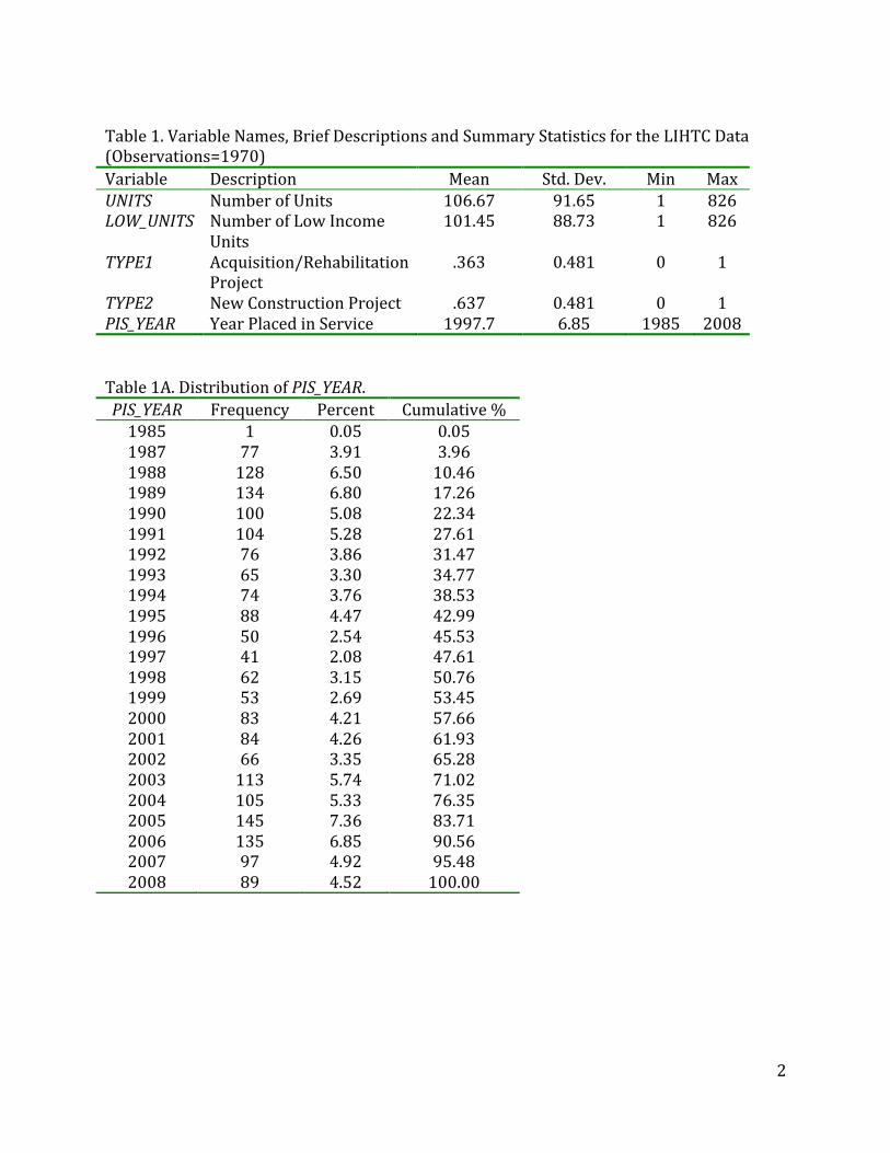
observations. Summary information about these data is presented in Table 1. Notice that the

total number of units and the number for low income are almost the same indicating that the

bulk of these projects provide housing for low-‐income tenants. Table 1A gives the frequency of

PIS_YEAR since the mean and standard deviation mask its actual distribution. Relatively

speaking and as noted in Figure 1, there were a lot of projects placed in service between 1988

and 1991 and then again between 2003 and 2007.

1 The US Department of Housing and Urban Development also maintains a database on LIHTC units but we used their data only for reconciling some addresses or missing values in the TDHCA data. Additionally, a critical variable for us is the year that the property in service (PIS_YEAR). Approximately 10% of our observations did not have this variable. Rather than delete the observations, we approximated the placed-‐in-‐service year by adding one year to the approval date for the financing. This algorithm is justified by looking at the relationship between approval dates and placed-‐in-‐service years for the observations that had good data in both fields.

The second source of data was the Texas Education Agency2. In particular, the TEA

maintains a multi-‐year, multi-‐table database on campuses that includes enrollments, student

demographics, number of teachers, staff and administrations, financials, and measures

achievement on TEA standardized tests.3 Additionally, and of particular interest, the TEA rates

each campus. The rankings generally fall into one of four categories Exemplary (RATING=4),

Recognized (RATING=3), Academically Acceptable (RATING=2) or Academically Unacceptable

(RATING=1). Ratings and other campus-‐level are available for 1996-‐2009, where, for example

2009 denoted the 2008-‐09 academic year. Other rating codes appear in the data such as “not

rated” but we did not use any of those observations. Additionally, the algorithm for making

ratings changed starting with 2004 so some care needs to be taken when comparing campuses

over time. Here, we coded 2003 as missing so that, in effect, our panel is 1996-‐2002 and 2004-‐

2009.

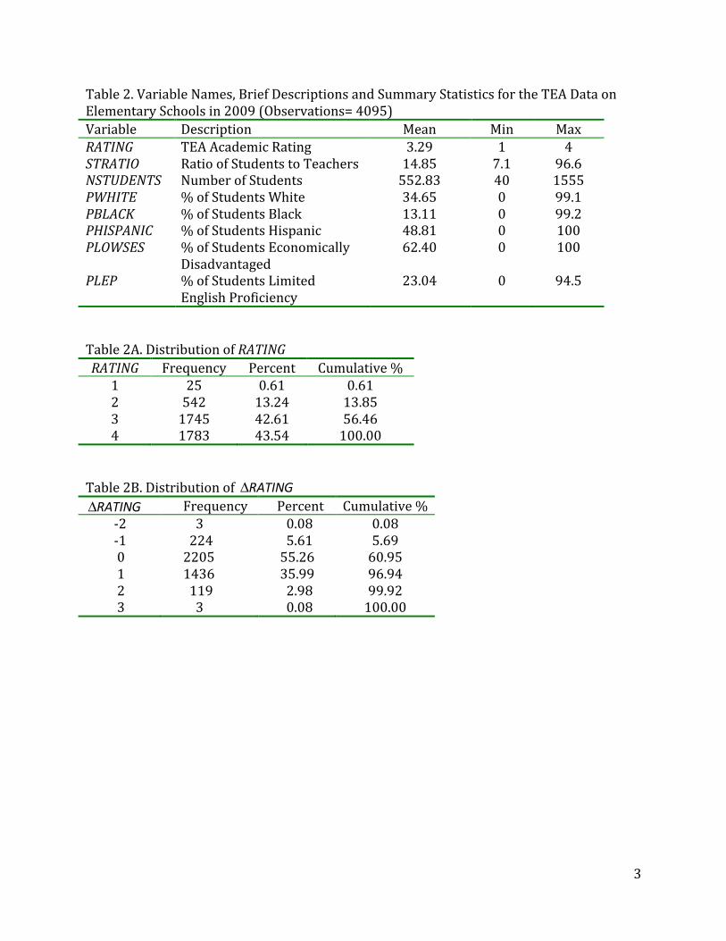
In Table 2 we present some of the school-‐level characteristics as well as the distribution

of RATING, and the change in the ratings ( ΔRATING ) for elementary schools in 2009. Note that

there are 4095 elementary school campuses with appropriate ratings 2009.4 The distributions

look similar for the other years. Not surprisingly most campuses are acceptable, recognized or

exemplary. A bit more curious is the almost even distribution between the last two categories.

The TDHCA data on LIHTC properties and the TEA data were spatially joined using a

three-‐step process. First, each LIHTC property was assigned its school district using a point-‐in-‐

polygon operation in a GIS. Next, for each year, each LIHTC that existed in that year was

assigned to its nearest campus, based on straight-‐line distance, which was in its district. Finally,

we determined the total units of LIHTC properties assigned to each school each year. It is

important note that no campus was assigned a LIHTC property that was outside of its school

district even if the LIHTC property happened to be within a mile.

2 See http://www.tea.state.tx.us. 3 The TEA web site also contains a GIS file with the district boundaries, and addresses for the campuses within districts. The campus-‐level data were address-‐geocoded in order to get the precise latitude and longitude for their locations. 4 Besides deleting cases without ratings, we deleted approximately 300 cases with anomalous data in terms of total number of students, total number of teachers and student teacher ratios.

The spatial merging of the data by year facilitated the creation of a panel of campuses

from 1996-‐2009 (but with 2004 missing) with campus-‐level TEA variables as well as the

existence and counts of LIHTC properties (and total units). The panel is unbalanced because of

new schools, school closures, and the fact that, for various reasons, not all schools are rated

each year. Still, it is a large dataset with the number of years equal to 13 and the number of

elementary schools approximately 4000. (Actual total N= 42,029.)

Analysis

Our goal is to investigate the direction and statistical significance of the impact of

changes in nearby LIHTC units on changes in ratings. With the panel of elementary schools,

presumably, we can identify these impacts using a couple of different strategies. One way is

estimate regressions with school fixed effects with ordered probit. However, we found with

that with ordered limited dependent variable this strategy simply took to long to be a

reasonable approach. Thus, we opted for regressing changes in the number of LIHTC units (

ΔUNITS ) on ΔRATING with controls for the changes in other potentially important time-‐

varying school-‐level characteristics that might impact academic ratings. Differencing the data

should remove the time-‐invariant effects. Since ΔRATING is also an ordinal categorical variable

(but with seven categories), we proceed by using ordered probit for the regressions.

In Table 3, we display the correlation coefficients for the main variables used in the

regressions. Note that we use “Δ ” for year-‐over-‐year change and the subscript “-‐1” to denote

a one lag. The surprising pattern in Table 3 is the apparent lack of any association between the

LIHTC variables and the campus-‐level student demographics. The highest correlation is 0.012

between the lag of the change in LIHTC units and the change in the percentage of students that

are economically disadvantaged. Given the purpose of the LIHTC program, expected to see

more movement in demographics as a result of the program. The lack of correlation is probably

an indication of just how small the housing program is. The student demographic variables are

correlated in predictable ways and they suggest that we probably will not be successful at

estimating independent effects for each variable. PLOWSES and PLEP go down when PWHITE

increases; and, of course, ΔSTRATIO and ΔNSTUDENTS are positively related.

Table 4 shows several models of ΔRATING . Model (1) is simply a bivariate specification

that indicates that the unconditional association between ΔRATING and ΔUNITS is positive,

meaning that a positive annual change in the number of LIHTC units is associated with a

positive change in the academic rating of the nearest elementary school. (The t-‐ratio is 1.45.)

The “Cuts” in Table 4 denote the estimated values of the underlying latent variable of the

ordered probit model, which we might think of as “academic improvement”. For example, in

Model (1) the assumed underlying equation is y* = 0.000444× ΔUNITS , where y

* is the

predicted value of the latent variable y ; hence, a value of y* < −3.849will be in the first

category of the observed variable-‐-‐ ΔRATING = −3 , while a value of y* > 3.619will be in the

highest category -‐-‐ ΔRATING = 3 (Greene 2000). The ordered probit model also implies a set of

marginal effects; i.e., the increment to the probability of being in one of the categories from an

increment in an independent variable. Once again, using the estimates in Model 1, we find that

the increments to the probabilities of being in categories 1-‐7 from a 100 increment in ΔUNITS

model are:

-‐0.000011, -‐0.0009, -‐0.0094, -‐0.0038, 0.0122, 0.002, 0.000021, respectively. In other

words, an increase in the number of LIHTC units nearby implies that the probability distribution

shifts in such a way that it is now more likely that the nearest school has a positive change in its

rating.5

Model (2) includes the one period lag of ΔUNITS . The idea here is to allow the impacts to take

longer than one year. Interestingly, Model (2) implies a larger contemporaneous effect with

some lingering negative effects of almost exactly the same magnitude and precision as the

coefficient on ΔUNITS . (The second lag—not displayed-‐-‐ is completely insignificant.) Thus, it

appears as though any initial positive impacts from LIHTC units are negated after a year.

5 The pattern of these probabilities does not change much over the different models as long as the means of the other independent variables are used to make the calculations. Thus, we do not present them for the other models.

Models (3) – (6) add sequentially ΔSTRATIO , ΔNSTUDENTS and their lags. If the positive

impact of LIHTC units is due to the extra resources associated with serving more children, we

would expect these terms to washout the effect. However, we see that for all models the

estimates on ΔUNITS are consistent. Not surprisingly, both ΔSTRATIO and its lag are negative.

Similarly, ΔNSTUDENTS is negative and it explains the contemporaneous student ratio effect.

However, the lag of the student teacher ratio remains robust even with the addition of the lag

of ΔNSTUDENTS . Evidently, a higher student teacher ratio will negatively effect ratings the

following year.

Table 5 shows four additional specifications labeled Models (7), (8), (9), and (10). In

these models we add changes in student characteristics in an attempt to explain away the

LIHTC findings. The new variables are changes in the percentage of the students that are

economically disadvantaged, white, and of limited English proficiency. Clearly, the change in

PWHITE dominates these effects but it does not have much impact on the first set of variables.

Hence, ΔUNITS , and ΔSTRATIO remain robust. (Of course, we know that ΔSTRATIO will be

affected by ΔNSTUDENTS .)

Discussion These preliminary results are intriguing for a couple of reasons. First, it is surprising that we

found any relationship at all between LIHTC units and school ratings. After all, compared to the

number of elementary schools, there aren’t a lot new LIHTC units each year. In other words,

the “treatment” is relatively small. Moreover, even using the ratings has an indicator of

academic success is problematic (Kane and Staiger 2002). It would not have been too surprising

if the models were completely insignificant. Second, the findings with respect to student-‐

teacher ratio, school size and percentage of the student body that is white make perfect sense,

giving some confidence in the overall structure of the model and help alleviate our overall

concerns about using the ratings data. Third, the findings with respect to LIHTC units offer

“food for thought” in the sense that they point toward alternative explanations for the

potential role played by LIHTC units.

For example, it seems as though the kids from LIHTC units give an initial bump (on

average) to nearby schools but that the effect is mitigated after one year. Is it possible that the

LIHTC kids are strong performers who, through peer, teacher, and other school-‐level effects,

tend back toward the mean of the school after a year or so? Alternatively, do the LIHTC results

simply pick up an external condition such as economic development? The idea would be that

economic development, being driven by rational developers, is driven toward positively

trending schools; hence, LIHTC units just so happen to appear simultaneously with increases in

ratings. However, after the development the school is different in some fashion and the ratings

tend to fall. At first glance this alternative explanation seems plausible. However, if it were

true, one would think that the changes in school demographics would wash out the lag on the

LIHTC terms. Yet, these are robust.

Perhaps this study suggests that it may be worth trying to conduct a student-‐level study

although it will be difficult to find the data. A student-‐level study would allow for more control

over the demographics and potentially allow us to determine differences in school

characteristics for kids who move into LIHTC properties. In this study, we are attempting to

infer something about the LIHTC kids by looking at changes in their nearest school.

In conclusion, it is probably worth stressing that the overall findings suggest that there is

very little impact from LIHTC units on neighborhood schools. This seems true regardless of the

explanation of how the effects are working.

References

Alexander, K. L., D. R. Entwisle, et al. (1996). "Children in Motion: School Transfers and Elementary School Performance." The Journal of Education Research 90(1): 3-‐12.

Bali, V. A. and R. M. Alvarez (2004). "The Race Gap in Student Achievement Scores: Longitudinal Evidence from a Racially Diverse School District." The Policy Studies Journal 32(3): 393-‐415.

Burke, M. A. and T. R. Sass (2008). Classroom peer effects and student achievement, Federal Reserve Bank of Boston.

Buron, L., S. Nolden, et al. (2000). Assessment of the Economic and Social Characteristics of LIHTC Residents and Neighborhoods.

Card, D. and J. Rothstein (2007). "Racial segregation and the black-‐white test score gap." Journal of Public Economics 91(11-‐12): 2158-‐2184.

Cooley, J. (2006). Desegregation and the Achievement Gap: Do Diverse Peers Help? Downs, A. (1982). "Creating more affordable housing." Journal of Housing 49(4): 174-‐183. Evans, W. N., W. E. Oates, et al. (1992). "Measuring Peer Group Effects: A Study of Teenage

Behavior." The Journal of Political Economy 100(5): 966-‐991. Ezzet-‐Lofstrom, R. and J. C. Murdoch (2007). "The Effect of Low-‐Income Housing Tax Credit

Units on Residential Property Values in Dallas County." Williams Review 2: 107-‐124. Finkel, M., C. G. Climaco, et al. (1996). Learning from each other: New ideas for managing the

Section 8 certifi cate and voucher program. Washington, DC, U.S. Department of Housing and Urban Development.

Greene, W. H. (2000). Econometric Analysis. Upper Saddle River, New Jersey, Prentice-‐Hall, Inc. Hanushek, E. A., J. F. Kain, et al. (2003). "Does Peer Ability Affect Student Achievement?"

Journal of Applied Econometrics 18(5): 527-‐544. Hanushek, E. A. and M. E. Raymond (2005). "Does School Accountability Lead to Improved

Student Performance?" Journal of Policy Analysis and Management 24(2): 297-‐327. Hoxby, C. (2000). Peer Effects in the Classroom: Learning from Gender and Race Variation.

NBER Working Paper Series. Jacob, B. A. and J. Ludwig (2009). Improving Educational Outcomes for Poor Children. Changing

Poverty, Changing Policies. M. Cancian and S. Danziger. New York, Russel Sage Foundation: 266-‐300.

Kane, T. J. and D. O. Staiger (2002). "The Promise and Pitfalls of Using Imprecise School Accountability Measures." Journal of Economic Perspectives 16(4): 91-‐114.

Lazear, E. P. (2001). "Educational Production." Quarterly Journal of Economics 116(3): 777-‐803. Lopez, R. and W. Di (2009). "Low-‐Income Housing Tax Credits in Texas: Achievements and

Challenges." Banking and Community Perspectives(2). Mao, M. X., M. D. Whitsett, et al. (1997). Student Mobility, Academic Performance, and School

Accountability. Nguyen, M. T. (2005). "Does Affordable Housing Detrimentally Affect Property Values? A

Review of the Literature." Journal of Planning Literature 20(1): 15-‐26. Ouazad, A. (2008). Assessed by a Teacher Like Me: Race, Gender, and Subjective Evaluations.

INSEAD Working Paper Series. Pendall, R. (1999). "Opposition to housing: NIMBY and beyond." Urban Affairs Review 35(1):

112-‐136. Rivkin, S. G., E. A. Hanushek, et al. (2005). "Teachers, Schools, and Academic Achievement."

Econometrica 73(2): 417-‐458. Scafidia, B., D. L. Sjoquistb, et al. (2007). "Race, Poverty, and Teacher Mobility." Economics of

Education Review 26: 145-‐159. Turner, M. A., S. Popkin, et al. (2000). Section 8 mobility and neighborhood health Washington,

DC, Urban Institute. Vigdor, J. and J. Ludwig (2007). SEGREGATION AND THE BLACK-‐WHITE TEST SCORE GAP. NBER

Working Paper Series.

1

Tables

2

Table 1. Variable Names, Brief Descriptions and Summary Statistics for the LIHTC Data (Observations=1970) Variable Description Mean Std. Dev. Min Max UNITS Number of Units 106.67 91.65 1 826 LOW_UNITS Number of Low Income

Units 101.45 88.73 1 826

TYPE1 Acquisition/Rehabilitation Project

.363 0.481 0 1

TYPE2 New Construction Project .637 0.481 0 1 PIS_YEAR Year Placed in Service 1997.7 6.85 1985 2008 Table 1A. Distribution of PIS_YEAR.

PIS_YEAR Frequency Percent Cumulative % 1985 1 0.05 0.05 1987 77 3.91 3.96 1988 128 6.50 10.46 1989 134 6.80 17.26 1990 100 5.08 22.34 1991 104 5.28 27.61 1992 76 3.86 31.47 1993 65 3.30 34.77 1994 74 3.76 38.53 1995 88 4.47 42.99 1996 50 2.54 45.53 1997 41 2.08 47.61 1998 62 3.15 50.76 1999 53 2.69 53.45 2000 83 4.21 57.66 2001 84 4.26 61.93 2002 66 3.35 65.28 2003 113 5.74 71.02 2004 105 5.33 76.35 2005 145 7.36 83.71 2006 135 6.85 90.56 2007 97 4.92 95.48 2008 89 4.52 100.00

3

Table 2. Variable Names, Brief Descriptions and Summary Statistics for the TEA Data on Elementary Schools in 2009 (Observations= 4095) Variable Description Mean Min Max RATING TEA Academic Rating 3.29 1 4 STRATIO Ratio of Students to Teachers 14.85 7.1 96.6 NSTUDENTS Number of Students 552.83 40 1555 PWHITE % of Students White 34.65 0 99.1 PBLACK % of Students Black 13.11 0 99.2 PHISPANIC % of Students Hispanic 48.81 0 100 PLOWSES % of Students Economically

Disadvantaged 62.40 0 100

PLEP % of Students Limited English Proficiency

23.04 0 94.5

Table 2A. Distribution of RATING RATING Frequency Percent Cumulative %

1 25 0.61 0.61 2 542 13.24 13.85 3 1745 42.61 56.46 4 1783 43.54 100.00

Table 2B. Distribution of ΔRATING ΔRATING Frequency Percent Cumulative % -‐2 3 0.08 0.08 -‐1 224 5.61 5.69 0 2205 55.26 60.95 1 1436 35.99 96.94 2 119 2.98 99.92 3 3 0.08 100.00

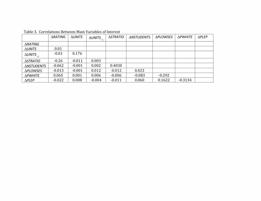
Table 3. Correlations Between Main Variables of Interest ΔRATING ΔUNITS

ΔUNITS−1 ΔSTRATIO ΔNSTUDENTS ΔPLOWSES ΔPWHITE ΔPLEP

ΔRATING ΔUNITS 0.01

ΔUNITS−1 -‐0.01 0.176

ΔSTRATIO -‐0.26 -‐0.011 0.003 ΔNSTUDENTS -‐0.062 -‐0.001 0.002 0.4030 ΔPLOWSES -‐0.013 -‐0.001 0.012 -‐0.012 0.023 ΔPWHITE 0.065 0.001 0.006 -‐0.006 -‐0.083 -‐0.292 ΔPLEP -‐0.022 0.008 -‐0.004 -‐0.011 0.060 0.1622 -‐0.3134

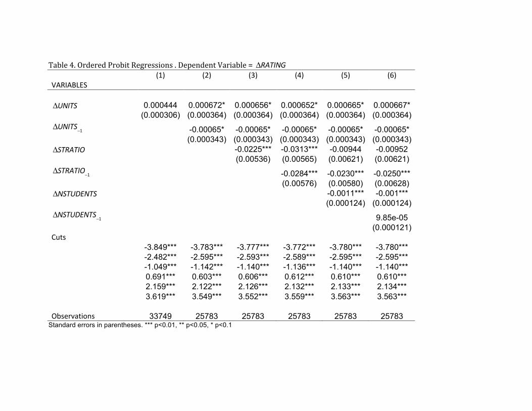
Table 4. Ordered Probit Regressions . Dependent Variable = ΔRATING (1) (2) (3) (4) (5) (6) VARIABLES

ΔUNITS 0.000444 0.000672* 0.000656* 0.000652* 0.000665* 0.000667* (0.000306) (0.000364) (0.000364) (0.000364) (0.000364) (0.000364)

ΔUNITS−1 -0.00065* -0.00065* -0.00065* -0.00065* -0.00065* (0.000343) (0.000343) (0.000343) (0.000343) (0.000343) ΔSTRATIO -0.0225*** -0.0313*** -0.00944 -0.00952 (0.00536) (0.00565) (0.00621) (0.00621)

ΔSTRATIO−1 -0.0284*** -0.0230*** -0.0250*** (0.00576) (0.00580) (0.00628) ΔNSTUDENTS -0.0011*** -0.001*** (0.000124) (0.000124)

ΔNSTUDENTS−1 9.85e-05 (0.000121) Cuts -3.849*** -3.783*** -3.777*** -3.772*** -3.780*** -3.780*** -2.482*** -2.595*** -2.593*** -2.589*** -2.595*** -2.595*** -1.049*** -1.142*** -1.140*** -1.136*** -1.140*** -1.140*** 0.691*** 0.603*** 0.606*** 0.612*** 0.610*** 0.610*** 2.159*** 2.122*** 2.126*** 2.132*** 2.133*** 2.134*** 3.619*** 3.549*** 3.552*** 3.559*** 3.563*** 3.563*** Observations 33749 25783 25783 25783 25783 25783

Standard errors in parentheses. *** p<0.01, ** p<0.05, * p<0.1

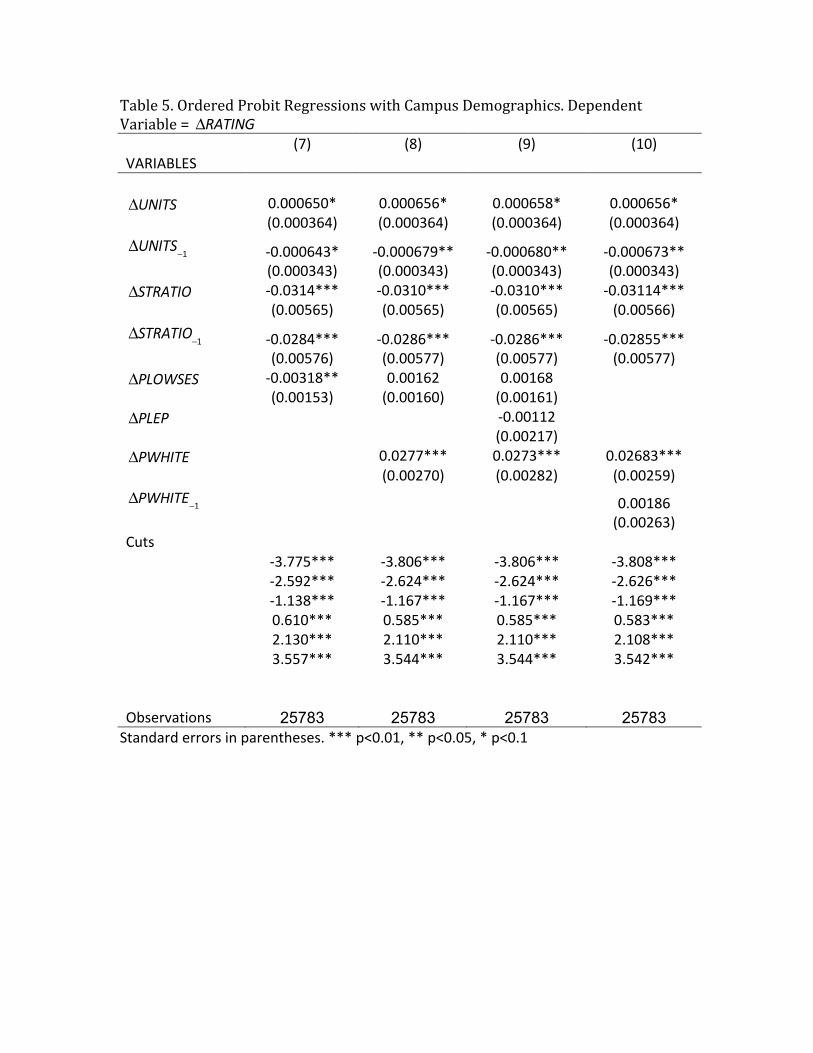
Table 5. Ordered Probit Regressions with Campus Demographics. Dependent Variable = ΔRATING (7) (8) (9) (10) VARIABLES

ΔUNITS 0.000650* 0.000656* 0.000658* 0.000656* (0.000364) (0.000364) (0.000364) (0.000364)

ΔUNITS−1 -‐0.000643* -‐0.000679** -‐0.000680** -‐0.000673** (0.000343) (0.000343) (0.000343) (0.000343)

ΔSTRATIO -‐0.0314*** -‐0.0310*** -‐0.0310*** -‐0.03114*** (0.00565) (0.00565) (0.00565) (0.00566)

ΔSTRATIO−1 -‐0.0284*** -‐0.0286*** -‐0.0286*** -‐0.02855*** (0.00576) (0.00577) (0.00577) (0.00577)

ΔPLOWSES -‐0.00318** 0.00162 0.00168 (0.00153) (0.00160) (0.00161)

ΔPLEP -‐0.00112 (0.00217)

ΔPWHITE 0.0277*** 0.0273*** 0.02683*** (0.00270) (0.00282) (0.00259)

ΔPWHITE−1 0.00186 (0.00263) Cuts -‐3.775*** -‐3.806*** -‐3.806*** -‐3.808*** -‐2.592*** -‐2.624*** -‐2.624*** -‐2.626*** -‐1.138*** -‐1.167*** -‐1.167*** -‐1.169*** 0.610*** 0.585*** 0.585*** 0.583*** 2.130*** 2.110*** 2.110*** 2.108*** 3.557*** 3.544*** 3.544*** 3.542*** Observations 25783 25783 25783 25783 Standard errors in parentheses. *** p<0.01, ** p<0.05, * p<0.1

AEA Jan paper - utdallas.edumurdoch/NeighborhoodChange/LIHTC/Di_Murdoch.… ·...

Documents

Transcript of AEA Jan paper - utdallas.edumurdoch/NeighborhoodChange/LIHTC/Di_Murdoch.… ·...