Application of the false discovery rate to microbial community comparison

james robert white, whitej@umd.edu,

Center for Bioinformatics and Computational Biology University of Maryland – College Park

College Park, MD 20742

Advisor: Mihai Pop, mpop@umiacs.umd.edu.

December 6th, 2007 Abstract We propose the development of new software to statistically determine differentially abundant taxa between two populations. Using only randomly selected 16S rRNAs from environmental samples, our goal is to assign each sequence to its appropriate taxon and analyze a taxa abundance matrix to find significantly overrepresented or underrepresented groups between two populations. Our problem is analogous to finding differentially expressed genes, and we aim to modify and implement methods already in practice in the microarray community. Specifically, we shall use the false discovery rate (FDR) and its corresponding measurement, the q-value, to control the number of false positives that frequently occur when performing multiple hypothesis tests.

Introduction • The 16S rRNA gene and data collection Currently, ~99% of all microbes cannot be isolated from their environments and cultured in a lab1. This statistic reveals our shallow understanding of the true complexity of microbial environments. Nevertheless, researchers are pushing to understand the structures of microbial communities in the rapidly expanding field of metagenomics. An increasing number of metagenomics studies focusing on species diversity within environments have been largely based on small subunit ribosomal RNA (SSU rRNA), particularly, the 16S rRNA gene. The 16S rRNA gene is ubiquitous to all known bacteria and archaea, and is highly conserved because of its essential function. However, there is enough divergence among these genes such that researchers can identify a species simply by sequencing its 16S gene. Typically, scientists take samples from an environment and extract DNA from captured microbes. Molecular biologists then sequence randomly selected 16S genes using PCR (polymerase chain reaction) and “universal” 16S primers. Note that the DNA of genes themselves is sequenced, not the mRNA transcript, thus there are no issues involving rates of transcription. Each 16S gene sequenced acts as a “bar code” or tag for a particular organism (fig. 1). Analyzing these genes, researchers have been able to describe the microflora of several environments2-12.

Figure 1 Metagenomic 16S rRNA sequencing. Single-celled organisms are collected from an environmental sample, and DNA is extracted. Universal PCR primers are used to amplify 16S rRNA genes from extracted DNA are sequenced. Each sequence is then classified to a particular taxon.

Several statistical software tools for 16S analysis have been developed such as DOTUR13, S-libshuff14, SONs15, UniFrac16, and TreeClimber17. Though these packages provide some information about community structure overlap and phylogenetic diversity, they are not designed for comparing hundreds of different communities simultaneously, and often fall short of providing researchers with enough information to make conclusions about environment composition. We seek to find out not if two populations are different, but exactly how they differ. Our objective is to determine which taxa in two populations are differentially abundant, that is, make up different proportions of the organisms in the environments. Our problem is

analogous to finding differentially expressed genes between two populations, a problem that has been researched for the past 10 years. Determining differentially expression can be easily conceptualized as a statistical hypothesis test. Consequently, statisticians working with microarrays have developed new methods for performing many hypothesis tests simultaneously. • Multiple hypothesis testing Over the past decade, significant attention has been given to multiple hypothesis testing, due in part to the development of high-throughput biological studies. For any single hypothesis test, there is a null hypothesis (H0) and an alternative hypothesis (HA). The goal is to correctly determine whether H0 or HA is true. H0 can be rejected or accepted depending on a measurement of significance such as a p-value and prior criteria set before the test. If one rejects the null hypothesis when it is true, this is a false positive (type I error). If one accepts the null when it is false, this is a false negative (type II error). Figure 2 provides an overview of the possible outcomes associated with performing M hypothesis tests. We denote the number of rejected hypotheses as Mr and the number of correctly rejected hypotheses as MrT. Note that we do not know MrT.

Figure 2 When performing M hypothesis tests, each test must accept or reject the null hypothesis H0. Of the number of tests that reject H0 (Mr), if some of the null hypotheses are in fact true (MrT), then this is type I error. Of the tests that accept H0, if some of these null hypotheses are actually false (MaF), then this is type II error.

One of the difficulties of multiple hypothesis testing is controlling type I error (i.e. reducing MrT). Traditionally, p-value cutoffs of 0.01 and 0.05 have been used for rejecting null hypotheses. However, when testing hundreds or thousands of null hypotheses, the typical p-value thresholds will result in a burdensome number of false positives. For example, if one performs 6000 tests, and rejects all null hypotheses with a p-value ≤ 0.05, one expects to have 300 false positives. This type I error rate is unacceptable for scientists who need to perform costly and time-consuming experiments. An intuitive modification would be to decrease the p-value cutoff to a very low value, thereby reducing the number of false positives, but this strict control results in a significant decrease in statistical power, leading to many incorrectly accepted null hypotheses. • The false discovery rate Recently, statisticians have succeeded in reducing the number of false positives by using the false discovery rate (FDR), which is defined to be the proportion of rejected null hypotheses that are false positives18. This is different from the false positive rate, which is defined as the

proportion of true null hypotheses that are rejected. As an example, a false positive rate of 1% means that 1% of all true null hypotheses are expected to be rejected. A false discovery rate of 1% means that 1% of all rejected null hypotheses are expected to be false positives. Each hypothesis test has an individual measure of the false positive rate called the p-value. A separate measure of significance called the q-value has been recently developed as an individual measure of the FDR for each test19. The difference between the q-value and the p-value is subtle but important. Rejecting all tests with a p-value ≤ α implies that one expects an overall false positive rate of α. If all tests with a q-value ≤ α are called significant, then one expects a false discovery rate of α. While the p-value provides information on all true null hypotheses, the q-value specifically provides information only on tests that reject H0. • Strategy The aim of this project is to apply the false discovery rate to metagenomic analysis in order to determine differentially abundant taxa between two environments. We have developed software that takes a species abundance matrix as input, and outputs an automated analysis of this matrix, isolating differentially abundant taxa using the q-values. Additionally, we have implemented a method for clustering species into higher groups (such as phyla, classes, orders, families, genera), and performing hypothesis tests on these larger categories of life. At species resolution, life forms may be too specific to the environment, and the true significance can be detected only by observing higher taxa. Methods • Taxa abundance matrix (TAM) This matrix is provided as input to our method. The ith row of the matrix represents a specific taxon, while the jth column represents a single replication of a treatment. Thus, the cell in the ith row and jth column is the total number of occurrences of taxon i in replication j (fig. 3). Every 16S rRNA sequence can only be counted once in the matrix, i.e. overlapping taxa are not allowed. We assume that there are only two treatments (e.g. sick and healthy), and that there are multiple replications per treatment. If there are g subjects in the first treatment, they are represented by the first g columns of the matrix, while the remaining columns represent subjects from the second treatment.

Figure 3 Format of the taxa abundance matrix. Each row represents a specific taxon, while each column represents a subject (replication). The frequency of the ith taxon in the jth subject (f(i,j)) is recorded in the corresponding cell of the matrix. If there are g subjects in the first treatment, they are represented by the first g columns of the matrix, while the remaining columns represent subjects from the second treatment.

• Taxonomic assignment There are several widely used methods for taxonomic assignment of 16S rRNA. Different approaches include sequence comparison, sequence composition, and phylogenetic analysis. In our experiments, we have assigned all 16S sequences to taxa using a naïve Bayesian classifier currently employed by the Ribosomal Database Project II (RDP)20. This software rapidly classifies sequences from kingdom to genus according to Bergey's Taxonomic Outline of the Prokaryotes (2nd ed., release 5.0, Springer-Verlag, New York, NY, 2004). Trained on ~23,000 pre-classified 16S sequences, the RDP classifier provides a statistical confidence (%) for each classification, and is available for use online (http://rdp.cme.msu.edu/classifier/classifier.jsp). • Matrix analysis We first compute the relative proportions of each taxon within each subject using the TAM. This results in a matrix of the same dimensions as the TAM, but the cell in the ith row and the jth column (which we shall denote aij) is the relative proportion of taxon i in subject j. For each taxon i, we calculate the mean proportion

!

x i1, and variance s2

i1 of treatment 1:

!

x i1 =1

n1

aij

j"treatment 1

#

si1

2 =1

n1$1

aij $ x i1( )2

j"treatment 1

#

Similarly, we calculate

!

x i2 and s2

i2 for treatment 2:

!

x i2 =1

n2

aij

j"treatment 2

#

si2

2 =1

n2$1

aij $ x i2( )2

j"treatment 2

#

Note that n1 and n2 are the number of subjects in treatment 1 and treatment 2, respectively. Finally, the two-sample t statistic for each taxon i is calculated as:

!

ti=

x i1" x

i2

si1

2

n1

+s

i2

2

n2

.

• Permuted p-value calculations We do not assume that the calculated t statistics follow a t distribution. Thus, we estimate the null distribution of ti nonparametrically using a permutation method described by Storey and Tibshirani (2003). Specifically, we randomly permute the treatment labels of the columns and recalculate the t statistics for the entire matrix. Note that the permutation maintains that there are n1 replications for treatment 1 and n2 replications for treatment 2. Repeating this procedure for B trials, we obtain B sets of t statistics: t1

0b, …, tM0b, b = 1, …, B, where M is the

number of taxa in the TAM. Memory space and computational efficiency should be considered when deciding how many permutations to use. If M = 1,000 and B = 10,000, then this algorithm will need to calculate 107 t statistics and store them in memory. Finally, the p-values for each taxon i, (i = 1, …, M) are calculated by pooling the null statistics:

!

pi =1

BM# j : t j

0b " ti , j =1,...,B{ }b=1

B

# .

• Q-value calculations

The following algorithm is adapted from Storey and Tibshirani (2003) for automated computation of q-values: Given an ordered list of p-values, p(1) ≤ p(2) ≤ … ≤ p(M), and a range of values λ = 0, 0.01, 0.02, …, 0.90, we compute

!

ˆ " 0#( ) =

#{p j > #}

m 1$ #( ).

Next, we fit

!

ˆ " 0#( ) with a cubic spline with 3 degrees of freedom, which we denote

!

ˆ f , and let

!

ˆ " 0

= ˆ f (1) . Finally, we estimate the q-value corresponding to each ordered p-value. First,

!

ˆ q p(m )( ) = min p(m ) " ˆ # 0, 1( ) . Then for i = m-1, m-2, …, 1,

!

ˆ q p(i)( ) = min ˆ " 0 #m # p( i)

i, ˆ q p( i+1)( )

$

% &

'

( ) .

Thus, the hypothesis test with p-value

!

p(i) has a corresponding q-value of

!

ˆ q p(i)( ) . Note that

this method yields conservative estimates of the true q-values, i.e.

!

ˆ q p(i)( ) " q p

( i)( ). • Computational implementation The algorithms designed for analysis of the taxa abundance matrix were implemented in R, a freely available statistical software package. Validation and application studies were performed on a MacBook Pro laptop (Mac OS X) with a dual core processor, 2.2GHz, and 2 GB of RAM. Validation • Hedenfalk dataset To validate our p-value and q-value calculations, we have analyzed a classic microarray dataset and compared it to a published q-value analysis of the same data19,21. Originally, 3,226 genes were studied using microarrays from 15 breast cancer subjects. Seven of these subjects had a genetic mutation called “BRCA1” while the other eight had a different genetic mutation, “BRCA2.” Both mutations are sources of hereditary breast cancer, and the initial study attempted to determine which genes could provide a distinctive diagnostic to identify hereditary breast cancer from microarray data. Storey and Tibshirani (2003) calculated high-quality p and q values for 3,170 of these candidate genes, where the null hypothesis for each test was that the expression level of the gene is the same in both populations. Using the same 3,170 genes as the previous q-value study, we computed permutation-based p-values and corresponding q-values for each gene. P-values were calculated using B = 200 permutations and a threshold of q ≤ 0.05 was used to call hypothesis tests significant. Furthermore, all genes called significant were collected and clustered using a UPGMA method and visualized in a heat map (using the R function heatmap). Figures 4 and 5 display the small differences between our calculated p and q values and the published study. These results validate our statistical calculations. Figure 6 displays the expression profiles for all genes we called significant.

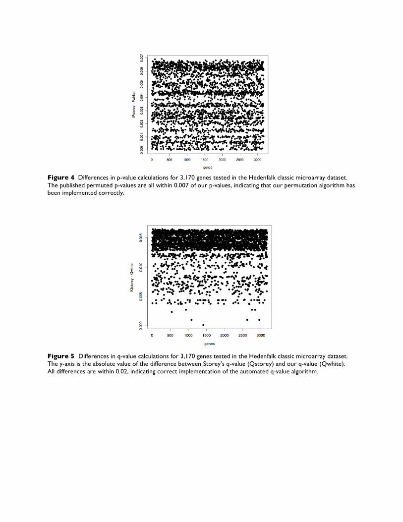
Figure 4 Differences in p-value calculations for 3,170 genes tested in the Hedenfalk classic microarray dataset. The published permuted p-values are all within 0.007 of our p-values, indicating that our permutation algorithm has been implemented correctly.

Figure 5 Differences in q-value calculations for 3,170 genes tested in the Hedenfalk classic microarray dataset. The y-axis is the absolute value of the difference between Storey’s q-value (Qstorey) and our q-value (Qwhite). All differences are within 0.02, indicating correct implementation of the automated q-value algorithm.

Figure 6 Expression profiles for genes called significant by thresholding q-values at α = 0.05. The first 7 columns represent profiles for the BRCA1 subjects, the last 8 columns are the BRCA2 subjects. The heatmap clearly displays the clusters of differentially expressed genes. We expect that 5% of these genes are false positives.

• Ley dataset As an initial application of our software to real 16S data, we have retrieved all sequences used in a recently published study of the human gut8. Using 12 obese subjects and 5 lean control subjects, Ley et al. found statistically significant differences in relative taxa abundance between the two groups: the Bacteroidetes and Firmicutes – the two dominant phyla in the human gut. This study found that the relative proportion of Bacteroidetes is decreased in obese people. Additionally, each obese subject was put on one of two calorie-restricted diets for one year, and as the obese subjects lost weight over the course of the year, their gut microflora began to resemble that of their lean counterparts. Our first goal was to reproduce the Ley et al. result that the two dominant phyla have significantly different relative abundances in lean and obese people. We classified 29,923 16S rRNA sequences, and created taxa abundance matrices comparing obese subjects to lean controls. Note that three of the control subjects were taken from another study4. A TAM corresponding to phyla was created containing observations of six distinct phyla, but the Bacteroidetes and Firmicutes dominated the samples. Since there were only six phyla observed, our algorithm only performed six hypothesis tests, so we decided to reject null hypotheses corresponding to a p-value of 0.05 or less. P-values were calculated using B = 1,000 permutations. Using our p-values, we were able to replicate the results given by the Ley study. The relative abundances of Bacteroidetes and Firmicutes were both significantly different between obese and lean subjects. Additionally, we discovered a third phylum was also significantly different

between the two treatments. Actinobacteria is a less dominant phylum making up less than 10% of the gut microbial population. Figure 7 displays the relative abundances of each significant taxa.

Figure 7 Relative proportions of significantly different taxa between obese and lean subjects, (p ≤ 0.05). Our results indicate that a third phylum, Actinobacteria, is also differentially abundant, adding to the results of the initial study.

Future studies The statistical analysis of microarray data is quite different from 16S rRNA frequency data. Continuous data and discrete data need different treatments. After consulting with two statisticians at the University of Maryland, I am directing my attention to the statistical methodology for handling the 16S data, rather than re-implementing the currently working software in C++. There are no major computational issues associated with the current implementation, and I plan to submit a small suite of tools to the BioConductor R project at the end of next semester. It is likely that I will develop several competing statistical methods for this analysis, and so I plan to create a sufficient simulation of a 16S study to determine which methods are more sensitive and more accurate. Additionally, I shall apply these methods to at least one additional metagenomic data set.

Proposed remaining schedule Milestone’s are highlighted in blue. 2007 December • Consider statistical methodology given sampling issues. • Develop at least two methodologies to compare. • Design broad simulation to test q-values vs. p-values. 2008 January • Finish broad simulation. • Finalize statistical methodology. • Finish application of software to Ley data. February • Apply best method to additional metagenomic data. • Develop documentation for software. March • Begin final report write-up. April • Complete final draft of report including edits from advisor. • Submit polished version of our software to BioConductor group. May • Deliver final report. • Final presentation (40 minutes). References 1. Tringe, S.G. & Rubin, E.M. Metagenomics: DNA sequencing of environmental samples. Nat

Rev Genet 6, 805-14 (2005). 2. Bik, E.M. et al. Molecular analysis of the bacterial microbiota in the human stomach. Proc

Natl Acad Sci U S A 103, 732-7 (2006). 3. Dunbar, J., Ticknor, L.O. & Kuske, C.R. Assessment of microbial diversity in four

southwestern United States soils by 16S rRNA gene terminal restriction fragment analysis. Appl Environ Microbiol 66, 2943-50 (2000).

4. Eckburg, P.B. et al. Diversity of the human intestinal microbial flora. Science 308, 1635-8 (2005).

5. Eder, W., Jahnke, L.L., Schmidt, M. & Huber, R. Microbial diversity of the brine-seawater interface of the Kebrit Deep, Red Sea, studied via 16S rRNA gene sequences and cultivation methods. Appl Environ Microbiol 67, 3077-85 (2001).

6. Gao, Z., Tseng, C.H., Pei, Z. & Blaser, M.J. Molecular analysis of human forearm superficial skin bacterial biota. Proc Natl Acad Sci U S A 104, 2927-32 (2007).

7. Garcia Martin, H. et al. Metagenomic analysis of two enhanced biological phosphorus removal (EBPR) sludge communities. Nat Biotechnol 24, 1263-9 (2006).

8. Ley, R.E., Turnbaugh, P.J., Klein, S. & Gordon, J.I. Microbial ecology: human gut microbes associated with obesity. Nature 444, 1022-3 (2006).

9. Palmer, C., Bik, E.M., Digiulio, D.B., Relman, D.A. & Brown, P.O. Development of the Human Infant Intestinal Microbiota. PLoS Biol 5, e177 (2007).

10. Schmidt, T.M., DeLong, E.F. & Pace, N.R. Analysis of a marine picoplankton community by 16S rRNA gene cloning and sequencing. J Bacteriol 173, 4371-8 (1991).

11. Sogin, M.L. et al. Microbial diversity in the deep sea and the underexplored "rare biosphere". Proc Natl Acad Sci U S A 103, 12115-20 (2006).

12. Venter, J.C. et al. Environmental genome shotgun sequencing of the Sargasso Sea. Science 304, 66-74 (2004).

13. Schloss, P.D. & Handelsman, J. Introducing DOTUR, a computer program for defining operational taxonomic units and estimating species richness. Appl Environ Microbiol 71, 1501-6 (2005).

14. Schloss, P.D., Larget, B.R. & Handelsman, J. Integration of microbial ecology and statistics: a test to compare gene libraries. Appl Environ Microbiol 70, 5485-92 (2004).

15. Schloss, P.D. & Handelsman, J. Introducing SONS, a tool for operational taxonomic unit-based comparisons of microbial community memberships and structures. Appl Environ Microbiol 72, 6773-9 (2006).

16. Lozupone, C. & Knight, R. UniFrac: a new phylogenetic method for comparing microbial communities. Appl Environ Microbiol 71, 8228-35 (2005).

17. Schloss, P.D. & Handelsman, J. Introducing TreeClimber, a test to compare microbial community structures. Appl Environ Microbiol 72, 2379-84 (2006).

18. Benjamini, Y. & Hochberg, Y. Controlling the False Discovery Rate - a Practical and Powerful Approach to Multiple Testing. Journal of the Royal Statistical Society Series B-Methodological 57, 289-300 (1995).

19. Storey, J.D. & Tibshirani, R. Statistical significance for genomewide studies. Proc Natl Acad Sci U S A 100, 9440-5 (2003).

20. Wang, Q., Garrity, G.M., Tiedje, J.M. & Cole, J.R. Naive Bayesian classifier for rapid assignment of rRNA sequences into the new bacterial taxonomy. Appl Environ Microbiol 73, 5261-7 (2007).

21. Hedenfalk, I. et al. Gene-expression profiles in hereditary breast cancer. N Engl J Med 344, 539-48 (2001).