Advanced Quantitative Methods - PS 401 Notes – Version as of 9/21/2000 Robert D. Duval WVU Dept of...
150
Advanced Quantitative Methods - PS 401 Notes – Version as of 9/21/2000 Robert D. Duval WVU Dept of Political Science Class Office 306E Woodburn 301A Woodburn TTh 11:30-12:45 T 2:00- 3:00 Th 1:00-3:00 Phone: 293-3811 x5299 293-4372 x13050
-
date post
19-Dec-2015 -
Category
Documents
-
view
214 -
download
1
Transcript of Advanced Quantitative Methods - PS 401 Notes – Version as of 9/21/2000 Robert D. Duval WVU Dept of...

Advanced Quantitative Methods - PS 401Notes – Version as of 9/21/2000
Robert D. Duval
WVU Dept of Political Science
Class Office
306E Woodburn 301A Woodburn
TTh 11:30-12:45 T 2:00-3:00
Th 1:00-3:00
Phone: 293-3811 x5299
293-4372 x13050
e-mail: [email protected]

Introduction
This course is about Regression analysis.• The principle method in the social science
Three basic parts to the course:• An introduction to the general Model• The formal assumptions and what they
mean.• Selected special topics

Syllabus
Required texts Additional readings Computer exercises Course requirements
• Midterm - in class, open book (30%)• Final - in class, open book (30%)• Research paper (30%)• Participation (10%)
http://www.polsci.wvu.edu/duval/ps401/401syl.html

Introduction: The General Linear Model
The General Linear Model is a phrase used to indicate a class of statistical models which include simple linear regression analysis.
Regression is the predominant statistical tool used in the social sciences due to its simplicity and versatility.
Also called Linear Regression Analysis.

Simple Linear Regression: The Basic Mathematical Model
Regression is based on the concept of the simple proportional relationship - also known as the straight line.
We can express this idea mathematically!• Theoretical aside: All theoretical statements
of relationship imply a mathematical theoretical structure.
• Just because it isn’t explicitly stated doesn’t mean that the math isn’t implicit in the language itself!
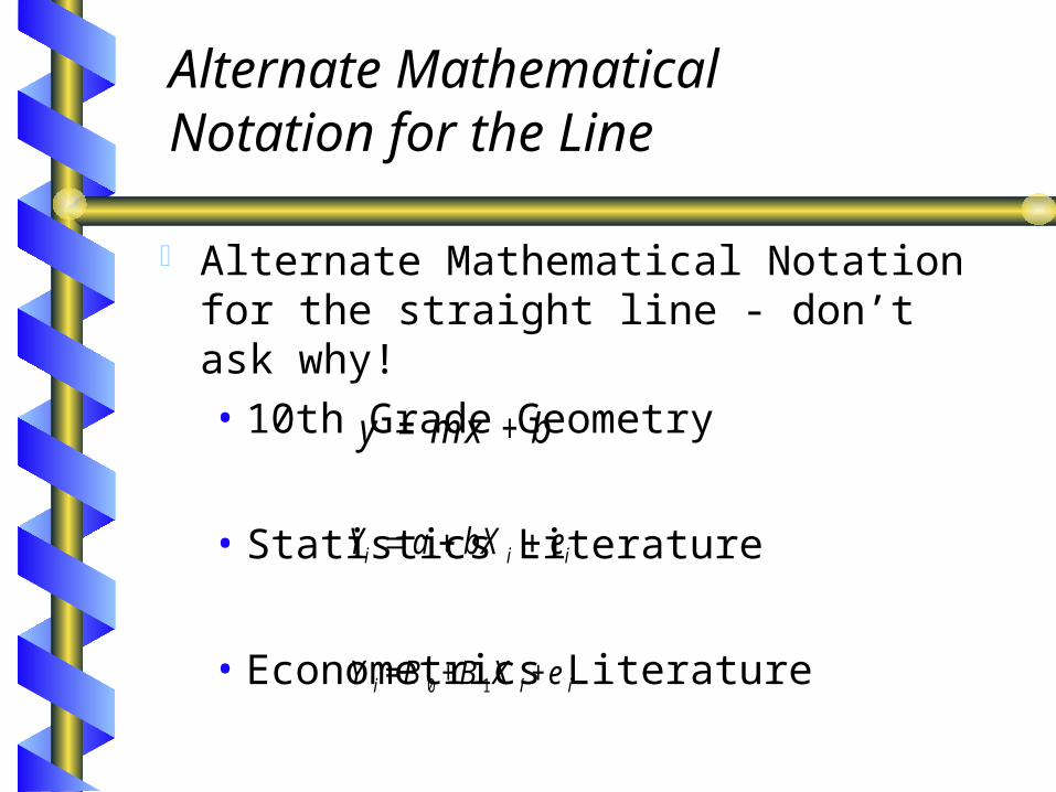
Alternate Mathematical Notation for the Line
Alternate Mathematical Notation for the straight line - don’t ask why!• 10th Grade Geometry
• Statistics Literature
• Econometrics Literature
y m x b= +
Y a bX ei i i
Y B B X ei i i= + +0 1

Alternate Mathematical Notation for the Line – cont.
These are all equivalent. We simply have to live with this inconsistency.
We won’t use the geometric tradition, and so you just need to remember that B0 and a are both the same thing.

Linear Regression: the Linguistic Interpretation
In general terms, the linear model states that the dependent variable is directly proportional to the value of the independent variable.
Thus if we state that some variable Y increases in direct proportion to some increase in X, we are stating a specific mathematical model of behavior - the linear model.
Hence, if we say that the crime rate goes up as unemployment goes up, we are stating a simple linear model.

Linear Regression:A Graphic Interpretation
The Straight Line
0
2
4
6
8
10
12
1 2 3 4 5 6 7 8 9 10
X
Y
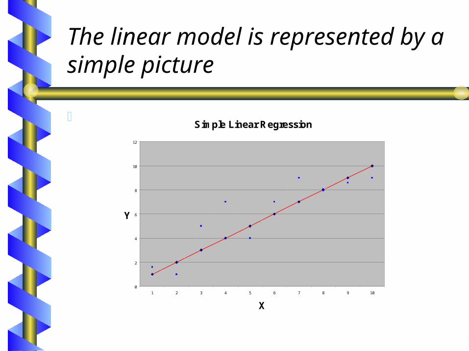
The linear model is represented by a simple picture
Simple Linear Regression
0
2
4
6
8
10
12
1 2 3 4 5 6 7 8 9 10
X
Y

The Mathematical Interpretation: The Meaning of the Regression Parameters
a = the intercept• the point where the line crosses the Y-axis.• (the value of the dependent variable when
all of the independent variables = 0) b = the slope
• the increase in the dependent variable per unit change in the independent variable (also known as the 'rise over the run')

The Error Term
Such models do not predict behavior perfectly.
So we must add a component to adjust or compensate for the errors in prediction.
Having fully described the linear model, the rest of the semester (as well as several more) will be spent of the error.

The Nature of Least Squares Estimation
There is 1 essential goal and there are 4 important concerns with any OLS Model

The 'Goal' of Ordinary Least Squares
Ordinary Least Squares (OLS) is a method of finding the linear model which minimizes the sum of the squared errors.
Such a model provides the best explanation/prediction of the data.

Why Least Squared error?
Why not simply minimum error? The error’s about the line sum to 0.0! Minimum absolute deviation (error) models
now exist, but they are mathematically cumbersome.
Try algebra with | Absolute Value | signs!

Other models are possible...
Best parabola...? • (i.e. nonlinear or curvilinear relationships)
Best maximum likelihood model ... ? Best expert system...? Complex Systems…?
• Chaos/Non-linear systems models• Catastrophe models• others

The Simple Linear Virtue
I think we over emphasize the linear model. It does, however, embody this rather important notion
that Y is proportional to X. As noted, we can state such relationships in simple
English.• As unemployment increases, so does the crime
rate.• As domestic conflict increased, national leaders
will seek to distract their populations by initiating foreign disputes.

The Notion of Linear Change
The linear aspect means that the same amount of increase in unemployment will have the same effect on crime at both low and high unemployment.
A nonlinear change would mean that as unemployment increases, its impact upon the crime rate might increase at higher unemployment levels.

Why squared error?
Because:• (1) the sum of the errors expressed as
deviations would be zero as it is with standard deviations, and
• (2) some feel that big errors should be more influential than small errors.
Therefore, we wish to find the values of a and b that produce the smallest sum of squared errors.

Minimizing the Sum of Squared Errors
Who put the Least in OLS In mathematical jargon we seek to minimize
the Unexplained Sum of Squares (USS), where:
U SS Y Y
e
i i
i
( )
2
2

The Parameter estimates
In order to do this, we must find parameter estimates which accomplish this minimization.
In calculus, if you wish to know when a function is at its minimum, you take the first derivative.
In this case we must take partial derivatives since we have two parameters (a & b) to worry about.
We will look closer at this and it’s not a pretty sight!

Why squared error?
Because
• (1) the sum of the errors expressed as deviations would be zero as it is with standard deviations, and
• (2) some feel that big errors should be more influential than small errors.
Therefore, we wish to find the values of a and b that produce the smallest sum of squared errors.

Decomposition of the error in LSDecomposition of the error in LS

Goodness of Fit
Since we are interested in how well the model performs at reducing error, we need to develop a means of assessing that error reduction. Since the mean of the dependent variable represents a good benchmark for comparing predictions, we calculate the improvement in the prediction of Yi relative to the mean of Y (the best guess of Y with no other information).

Sum of Squares Terminology
In mathematical jargon we seek to minimize the Unexplained Sum of Squares (USS), where:
U SS Y Y
e
i i
i
( )
2
2

Sums of Squares
This gives us the following 'sum-of-squares' measures:
Total Variation = Explained Variation + Unexplained Variation
TSS Tota l Sum Squares Y Y
ESS Exp la ined Sum of Squares Y Y
i
i
( )
( )
2
2

Sums of Squares Confusion
Note: Occasionally you will run across ESS and RSS which generate confusion since they can be used interchangeably. ESS can be error sums-of-squares or estimated or explained SSQ. Likewise RSS can be residual SSQ or regression SSQ. Hence the use of USS for Unexplained SSQ in this treatment.

The Parameter estimates
In order to do this, we must find parameter estimates which accomplish this minimization.
In calculus, if you wish to know when a function is at its minimum, you take the first derivative.
In this case we must take partial derivatives since we have two parameters to worry about.

Deriving the Parameter Estimates
Since
We can take the partial derivative with respect to a and b
U SS Y Y
e
Y a bX
i i
i
i i
( )
( )
2
2
2
USS
aY a bX
USS
bY a bX X
i i
i i i
2 1
2
( ) ( )
( ) ( )

Deriving the Parameter Estimates (cont.)
Which simplifies toWhich simplifies to
We also set these derivatives to 0 to indicate We also set these derivatives to 0 to indicate that we are at a minimum.that we are at a minimum.
USS
aY a bX
USS
bX Y a bX
i i
i i i
2 0
2 0
( )
( )

Deriving the Parameter Estimates (cont.)
We now add a “hat” to the parameters to We now add a “hat” to the parameters to indicate that the results are estimators and .indicate that the results are estimators and .
We also Set these derivatives equal to zero.
USS
aY a b X
USS
bX Y a b X
i i
i i i
2 0
2 0
( )
( )

Deriving the Parameter Estimates (cont.)
Dividing through by -2 and rearranging terms, we get
Y an b X
X Y a X b X
i i
i i i i
( ) ,
( ) ( )2

Deriving the Parameter Estimates (cont.)
We can solve these equations simultaneously to get our estimators.
bn X Y X Y
n X X
X X Y Y
X X
a Y b X
i i i i
i i
i i
i
1 2 2
2
1
( )
( )( )
( )

Deriving the Parameter Estimates (cont.)
The estimator for a which shows that the regression line always goes through the point which is the intersection of the two means.
This formula is quite manageable for bivariate regression. If there are two or more independent variables, the formula for b2, etc. becomes unmanageable!

Tests of Inference
t-tests for coefficients F-test for entire model

T-TestsT-Tests
Since we wish to make probability statements Since we wish to make probability statements about our model, we must do tests of about our model, we must do tests of inference.inference.
Fortunately,Fortunately,
B
set
Bn 2

This gives us the F test:

Measures of Goodness of fit
The Correlation coefficient r-squared

The correlation coefficient
A measure of how close the residuals are to the regression line
It ranges between -1.0 and +1.0 It is closely related to the slope.

R2 (r-square)
The r2 (or R-square) is also called the coefficient of determination.
rESS
TSSUSS
TSS
2
1

Tests of Inference
t-tests for coefficients F-test for entire model Since we are interested in how well the model
performs at reducing error, we need to develop a means of assessing that error reduction. Since the mean of the dependent variable represents a good benchmark for comparing predictions, we calculate the improvement in the prediction of Yi relative to the mean of Y (the best guess of Y with no other information).

Goodness of fit
The correlation coefficient
• A measure of how close the residuals are to the regression lineIt ranges between -1.0 and +1.0
r2 (r-square)
• The r-square (or R-square) is also called the coefficient of determination

The assumptions of the model
We will spend the next 4 weeks on this!

The Multiple Regression Model The Scalar Version
The basic multiple regression model is a simple extension of the bivariate equation. by adding extra independent variables, we are creating a multiple-dimensioned space, where the model fit is a some appropriate space. For instance, if there are two independent variables, we are fitting the points to a ‘plane in space’.

The Scalar EquationThe Scalar Equation
The basic linear model:The basic linear model:
Y a b X b X b X ei i i k k i i 1 1 2 2 . . .

The Matrix Model
The multiple regression model may be easily represented in matrix terms.
Where the Y, X, B and e are all matrices of data, coefficients, or residuals
Y XB e

The Matrix Model (cont.)The Matrix Model (cont.)
The matrices in are represented The matrices in are represented byby
Note that we postmultiply X by B since this order makes them conformable.
Y
Y
Y
Yn
1
2
X
X X X
X X X
X X X
ik
k
n n nk
11 1 2
2 1 2 2 2
1 2
. . .
. . .
. . . . . . . . . . . .
. . .
B
B
B
B k
1
2 e
e
e
en
1
2
Y XB e

Assumptions of the modelScalar Version
The OLS model has seven fundamental assumptions. These assumptions form the foundation for all regression analysis. Failure of a model to conform to these assumptions frequently presents severe problems for estimation and inference.

The Assumptions of the ModelScalar Version (cont.)
• 1. The ei's are normally distributed.
• 2. E(ei) = 0
• 3. E(ei2) = 2
• 4. E(eiej) = 0 (ij)
• 5. X's are nonstochastic with values fixed in repeated samples and (Xik-Xbark)2/n is a finite nonzero number.
• 6. The number of observations is greater than the number of coefficients estimated.
• 7. No exact linear relationship exists between any of the explanatory variables.

The Assumptions of the ModelThe English Version
The errors have a normal distribution.The errors have a normal distribution. The residuals are heteroskedastic.The residuals are heteroskedastic. There is no serial correlation.There is no serial correlation. There is no multicollinearity.There is no multicollinearity. The X’s are fixed. (non-stochastic)The X’s are fixed. (non-stochastic) There are more data points than unknowns.There are more data points than unknowns. The model is linear.The model is linear.
OK…so it’s not really English….OK…so it’s not really English….

The Assumptions of the Model: The Matrix Version
These same assumptions expressed in matrix format are:
• 1. e N(0,)
• 2. = 2I
• 3. The elements of X are fixed in repeated samples and (1/ n)X'X is nonsingular and its elements are finite

Extra Material on OLS: The Adjusted R2
Since R2 always increases with the addition of a new variable, the adjusted R2 compensates for added explanatory variables.
Extra Material on OLS: The F-test
In addition, the F test for the entire model must be adjusted to compensate for the changed degrees of freedom.
Note that F increases as n or R2 increases and decreases as k increasesAdding a variable will always increase R2, but not necessarily adjusted R2 or F. In addition values of adjusted R2 below 0.0 are possible.

Derivation of B's in matrix notation
Skip this material in PS 401 Given the matrix algebra model
1.33 we can replicate the least squares normal equations in matrix format.
We need to minimize e¢e, which is the sum of squared errors.1.34
Setting the derivative equal to 0 we get
1.35 1.36 1.37 1.38 Note that X’X is called the sums-of-squares and cross-products
matrix.

Properties of Estimators ()
Since we are concerned with error, we will be concerned with those properties of estimators which have to do with the errors produced by the estimates - the s

Types of estimator error
Estimators are seldom exactly correct due to any number of reasons, most notably sampling error and biased selection. There are several important concepts that we need to understand in examining how well estimators do their job.

Sampling error
Sampling error is simply the difference between the true value of a parameter and its estimate in any given sample.
This sampling error means that an estimator will vary from sample to sample and therefore estimators have variance.
Sampling E rror
Var E E E E( ) [ ( )] ( ) [ ( )] 2 2 2 2

Bias
The bias of an estimate is the difference between its expected value and its true value.
If the estimator is always low (or high) then the estimator is biased.
An estimator is unbiased if
And
E ( )
B ias E ( )

Mean Squared Error
The mean square error (MSE) is different from the estimator’s variance in that the variance measures dispersion about the estimated parameter while mean squared error measures the dispersion about the true parameter.
If the estimator is unbiased then the variance and MSE are the same.
M ean square error E ( ) 2

Mean Squared Error (cont.)
The MSE is important for time series and forecasting since it allows for both bias and efficiency:
For instance These concepts lead us to look at the properties of
estimators. Estimators may behave differently in large and small samples, so we look at both the small and large (asymptotic) sample properties.
M S E = v arian ce + (b ias) 2

Small Sample Properties
These are the ideal properties. We desire these to hold.
• Bias
• Efficiency
• Best Linear Unbiased Estimator

Bias
A parameter is unbiased if
In other words, the average value of the estimator in repreated sampling equals the true parameter.
Note that whether an estimator is biased or not implies nothing about its dispersion.
E ( )

Efficiency
An estimator is efficient if it is unbiased and where its variance is less than any other unbiased estimator of the parameter.
• Is unbiased;
• Var( ) Var ( ) where is any other unbiased estimator of
There might be instances in which we might choose a biased estimator, if it has a smaller variance.
~
~

BLUE (Best Linear Unbiased Estimate)
An estimator is described as a BLUE estimator if it is
• is a linear function
• is unbiased
• Var( ) Var ( ) where is any other linear unbiased estimator of
•
~~

What is a linear estimator?
Note that the sample mean is an example of a linear estimator.

Asymptotic (Large Sample) Properties
Asymptotically unbiased Consistency Asymptotic efficiency

Asymptotic bias
An estimator is unbiased if

Consistency
The point at which a distribution collapses is called the probability limit (plim)If the bias and variance both decrease as gets larger, the estimator is consistent.

Asymptotic efficiency
An estimator is asymptotically efficient if
• asymptotic distribution with finite mean and variance
• is consistent
• no other estimator has smaller asymptotic variance

Rifle and Target Analogy
Small sample properties– Bias The shots cluster around some spot other
than the bull’s-eye)
– Efficient: When one rifle’s cluster is smaller than another’s.
– BLUE - Smallest scatter for rifles of a particular type of simple construction

Rifle and Target Analogy (cont.)
Asymptotic properties
• Think of increased sample size as getting closer to the target. When all of the assumptions of the OLS model hold its estimators are:
– unbiased
– Minimum variance, and
– BLUE

Assumption Violations: How we will approach the question.
Definition Implications Causes Tests Remedies

Non-zero Mean for the residuals (Definition)
Definition:
• The residuals have a mean other than 0.0.
• Note that this refers to the true residuals. Hence the estimated residuals have a mean of 0.0, while the true residuals are non-zero.

Non-zero Mean for the residuals (Implications)
The true regression line is
Therefore the intercept is biased. The slope, b, is unbiased. There ia also no
way of separating out a and .
Y a bXi i e

Non-zero Mean for the residuals (Causes, Tests, Remedies)
CausesCauses: Non-zero means result from some : Non-zero means result from some form of specification error. Something has form of specification error. Something has been omitted from the model which accounts been omitted from the model which accounts for that mean in the estimation.for that mean in the estimation.
We will discuss We will discuss TestsTests and and RemediesRemedies when when we look closely at Specification errors.we look closely at Specification errors.

Non-normally distributed errors : Definition
The residuals are not NID(0,)
0.0
8.8
17.5
26.3
35.0
-1000.0 -250.0 500.0 1250.0 2000.0
Histogram of Residuals of rate90
Residuals of rate90
Count
Normality Tests SectionAssumption Value Probability Decision(5%)Skewness 5.1766 0.000000 RejectedKurtosis 4.6390 0.000004 RejectedOmnibus 48.3172 0.000000 Rejected

Non-normally distributed errors : Implications
The existence of residuals which are not normally distributed has several implications.
• First is that it implies that the model is to some degree misspecified.
• A collection of truly stochastic disturbances should have a normal distribution. The central limit theorem states that as the number of random variables increases, the sum of their distributions tends to be a normal distribution.

Non-normally distributed errors : Implications (cont.)
If the residuals are not normally distributed, then the estimators of a and b are also not normally distributed.
Estimates are, however, still BLUE. Estimates are unbiased and have minimum variance. They are no longer efficient, even though they are
asymptotically unbiased and consistent. It is only our hypothesis tests which are suspect.

Non-normally distributed errors: Causes
Generally causes by a misspecification error.Generally causes by a misspecification error. Usually an omitted variable.Usually an omitted variable. Can also result from Can also result from
• Outliers in data.Outliers in data.• Wrong functional form.Wrong functional form.

Non-normally distributed errors : Tests for non-normality
Chi-Square goodness of fit• Since the cumulative normal frequency distribution
has a chi-square distribution, we can test for the normality of the error terms using a standard chi-square statistic.
• We take our residuals, group them, and count how many occur in each group, along with how many we would expect in each group.

Non-normally distributed errors : Tests for non-normality (cont.)
• We then calculate the simple 2 statistic.
• This statistic has (N-1) degrees of freedom, where N is the number of classes.
2
2
1
O E
Ei i
ii
k

Non-normally distributed errors : Tests for non-normality (cont.)
Jarque-Bera test
• This test examines both the skewness and kurtosis of a distribution to test for normality.
• Where S is the skewness and K is the kurtosis of the residuals.
• JB has a 2 distribution with 2 df.
JB nS K
2 2
6
3
2 4
( )

Non-normally distributed errors: Remedies
Try to modify your theory. Omitted variable? Outlier needing specification?
Modify your functional form by taking some variance transforming step such as square root, exponentiation, logs, etc.
• Be mindful that you are changing the nature of the model.
Bootstrap it!

Multicollinearity: Definition
Multicollinearity is the condition where the independent variables are related to each other. Causation is not implied by multicollinearity.
As any two (or more) variables become more and more closely correlated, the condition worsens, and ‘approaches singularity’.
Since the X's are supposed to be fixed, this a sample problem.
Since multicollinearity is almost always present, it is a problem of degree, not merely existence.

Multicollinearity: Implications
Consider the following cases
• A) No multicollinearity– The regression would appear to be identical to separate bivariate regressions
This produces variances which are biased upward (too large) making t-tests too small.For multiple regression this satisfies the assumption.
• B) Perfect Multicollinearity– Some variable Xi is a perfect linear combination of one or more other variables Xj, therefore X'X is
singular, and |X'X| = 0.
– A model cannot be estimated under such circumstances. The computer dies.
• C. A high degree of Multicollinearity– When the independent variables are highly correlated the variances and covariances of the Bi's are
inflated (t ratio's are lower) and R2 tends to be high as well.
– The B's are unbiased (but perhaps useless due to their imprecise measurement as a result of their variances being too large). In fact there are still BLUE.
– OLS estimates tend to be sensitive to small changes in the data.
– Relevant variables may be discarded

Multicollinearity: Implications
Consider the following cases
• A) No multicollinearity– The regression would appear to be identical to
separate bivariate regressions
– This produces variances which are biased upward (too large) making t-tests too small.
– For multiple regression this satisfies the assumption.

Multicollinearity: Implications (cont.)
• B) Perfect Multicollinearity
– Some variable Xi is a perfect linear combination of one or more other variables Xj, therefore X'X is singular, and |X'X| = 0.
– This is matrix algebra notation. It means that one variable is a perfect linear function of another. (e.g. X2 = X1+3.2)
– A model cannot be estimated under such circumstances. The computer dies.

Multicollinearity: Implications (cont.)
• C. A high degree of Multicollinearity– When the independent variables are highly correlated the
variances and covariances of the Bi's are inflated (t ratio's are lower) and R2 tends to be high as well.
– The B's are unbiased (but perhaps useless due to their imprecise measurement as a result of their variances being too large). In fact they are still BLUE.
– OLS estimates tend to be sensitive to small changes in the data.
– Relevant variables may be discarded.
Multicollinearity: Causes
Sampling mechanism.Poorly constructed design & measurement scheme or limited range.
Statistical model specification: adding polynomial terms or trend indicators.
Too many variables in the model - the model is overdetermined.
Theoretical specification is wrong. Inappropriate construction of theory or even measurement

Multicollinearity: Tests/Indicators
|X'X| = approaches 0
• Since the determinant is a function of variable scale, this measure doesn't help a whole lot. We could, however, use the determinant of the correlation matrix and therefore bound the range from 0. to 1.0

Multicollinearity: Tests/Indicators (cont.)
Tolerance:
• If the tolerance equals 1, the variables are unrelated. If TOLj = 0, then they are perfectly correlated.
– Variance Inflation Factors (VIFs)
– Tolerance
V IFR k
1
1 2
TO L R V IFj j j 1 12 ( / ( ))

Interpreting VIFsInterpreting VIFs
No multicollinearity produces VIFs = 1.0No multicollinearity produces VIFs = 1.0 If the VIF is greater than 10.0, then If the VIF is greater than 10.0, then
multicollinearity is probably severe. 90% of multicollinearity is probably severe. 90% of the variance of Xthe variance of X jj is explained by the other is explained by the other
X’s.X’s. In small samples, a VIF of about 5.0 may In small samples, a VIF of about 5.0 may
indicate problemsindicate problems

Multicollinearity: Tests/Indicators (cont.)
R2 deletes - tries all possible models of X's and by includes/ excludes based on small changes in R2 with the inclusion/omission of the variables (taken 1 at a time)
F is significant, But no t value is. Adjusted R2 declines with a new variable Multicollinearity is of concern when either

Multicollinearity: Tests/Indicators (cont.)
I would avoid the rule of thumb
Beta's are > 1.0 or < -1.0 Sign changes occur with the introduction of a
new variable The R2 is high, but few t-ratios are. Eigenvalues and Condition Index - If this topic
is beyond Gujarati, it’s beyond me.

Multicollinearity: Remedies
Increase sample size Omit Variables Scale Construction/Transformation Factor Analysis Constrain the estimation. Such as the case
where you can set the value of one coefficient relative to another.

Multicollinearity: Remedies (cont.)
Change design (LISREL maybe or Pooled cross-sectional Time series)
Ridge Regression
• This technique introduces a small amount of bias into the coefficients to reduce their variance.
Ignore it - report adjusted r2 and claim it warrants retention in the model.

Heteroskedasticity: Definition
Heteroskedasticity is a problem where the error terms do not have a constant variance.
That is, they may have a larger variance when values of some Xi (or the Yi’s themselves) are large (or small).
E e i i( )2 2

Heteroskedasticity: Definition
This often gives the plots of the residuals by the dependent variable or appropriate independent variables a characteristic fan or funnel shape.
0
20
40
60
80
100
120
140
160
180
0 50 100 150
Series1

Heteroskedasticity: Implications
The regression B's are unbiased. But they are no longer the best estimator.
They are not BLUE (not minimum variance - hence not efficient).
They are, however, consistent.

Heteroskedasticity: Implications (cont.)
The estimator variances are not asymptotically efficient, and they are biased.
• So confidence intervals are invalid.
• What do we know about the bias of the variance?
• If Yi is positively correlated with ei, bias is negative - (hence t values will be too large.)
• With positive bias many t's too small.

Heteroskedasticity: Implications (cont.)
Types of Heteroskedasticity
• There are a number of types of heteroskedasticity.
– Additive
– Multiplicative
– ARCH (Autoregressive conditional heteroskedastic) - a time series problem.

Heteroskedasticity: Causes
It may be caused by:
• Model misspecification - omitted variable or improper functional form.
• Learning behaviors across time
• Changes in data collection or definitions.
• Outliers or breakdown in model.– Frequently observed in cross sectional data sets
where demographics are involved (population, GNP, etc).

Heteroskedasticity: Tests
Informal Methods
• Graph the data and look for patterns!

Heteroskedasticity: Tests (cont.)
Park test
• As an exploratory test, log the residuals and regress them on the logged values of the suspected independent variable.
• If the B is significant, then heteroskedasticity may be a problem.
ln ln ln
ln
u B X v
a B X vi i i
i i
2 2

Heteroskedasticity: Tests (cont.)
Glejser Test
• This test is quite similar to the park test, except that it uses the absolute values of the residuals, and a variety of transformed X’s.
• A significant B2 indicated Heteroskedasticity.
• Easy test, but has problems.
u B B X v
u B B X v
u B BX
v
i i i
i i i
ii
i
1 2
1 2
1 2
1
u B BX
v
u B B X v
u B B X v
ii
i
i i i
i i i
1 2
1 2
1 22
1

Heteroskedasticity: Tests (cont.)
Goldfeld-Quandt test
• Order the n cases by the X that you think is correlated with ei
2.
• Drop a section of c cases out of the middle(one-fifth is a reasonable number).
• Run separate regressions on both upper and lower samples.

Heteroskedasticity: Tests (cont.)
Goldfeld-Quandt test (cont.) Do F-test for difference in error variances
F has (n - c - 2k)/2 degrees of freedom for each

Heteroskedasticity: Tests (cont.)
Breusch-Pagan-Godfrey Test (Lagrangian Multiplier test)• Estimate model with OLS• Obtain
• Construct variables
nui /~ 22
22iii up ~/ˆ

Heteroskedasticity: Tests (cont.)
Breusch-Pagan-Godfrey Test (cont.)
• Regress pi on the X (and other?!) variables
• Calculate
• Note that
mimiii ZZZp ...33221
)(ESS2
1
21 m

Heteroskedasticity: Tests (cont.)
White’s Generalized Heteroskedasticity testWhite’s Generalized Heteroskedasticity test• Estimate model with OLS and obtain
residuals• Run the following auxiliary regression
• Higher powers may also be used, along with more X’s
)(ESS2
1

Heteroskedasticity: Tests (cont.)
White’s Generalized Heteroskedasticity test White’s Generalized Heteroskedasticity test (cont.)(cont.)• Note thatNote that
• The degrees of freedom is the number of The degrees of freedom is the number of coefficients estimated above.coefficients estimated above.
22 Rn

Heteroskedasticity: Remedies
GLS• We will cover this after autocorrelation
Weighted Least Squares
• si2 is a consistent estimator of si
2
• use same formula (BLUE) to get a + ß

Iteratively weighted least squares (IWLS)
• Uses BLUE• The Variance equals• Obtain estimates of and using OLS • Use these to get "1st round" estimates of si
2
• Using formula above replace wi with 1/ si2 and
obtain new estimates for a and ß. • Use these to re-estimate • Repeat Step 2 until a and ß converge.

Heteroskedasticity: Remedies (cont.)
Whites’s corrected standard errors
Discussion beyond this course… Some software will calculate these.
• (SHAZAM,TSP)

Autocorrelation: Definition
Autocorrelation is simply the presence of standard correlation between adjacent residuals.
If a residual is negative (positive) then it’s neighbors tend to also be negative (positive).
Most often autocorrelation is between adjacent observations, however, lagged or seasonal patterns can also occur.
Autocorrelation is also usually a function of order by time, but it can occur for other orders as well.

Autocorrelation: Definition (cont.)
The assumption violated is
Meaning that the Pearson’s r between the residuals from OLS and the same residuals lagged on period is non-zero.
0)( jieeE

Autocorrelation: Definition (cont.)
Most autocorrelation is what we call 1st order autocorrelation, meaning that the residuals are related to their contiguous values
For instance:

Autocorrelation: Definition (cont.)
Types of Autocorrelation
• Autoregressive processes
• Moving Averages

Autocorrelation: Definition (cont.)
Autoregressive processes AR(p)
• The residuals are related to their preceding values.
• This is classic 1st order autocorrelation
ttt uee 1

Autocorrelation: Definition (cont.)
Autoregressive processes (cont.)
• In 2nd order autocorrelation the residuals are related to their t-2 values as well
• Larger order processes may occur as well
tptpttt ueeee ...2211
tttt ueee 2211

Autocorrelation: Definition (cont.)
Moving Average Processes MA(q)
The error term is a function of some random error plus a portion of the previous random error.
1 ttt uue

Autocorrelation: Definition (cont.)
Moving Average Processes (cont. Higher order processes for MA(q) also exist.
The error term is a function of some random error plus a portion of the previous random error.
qtqtttt uuuue ...2211

Autocorrelation: Definition (cont.)
Mixed processes ARMA(p,q)
The error term is a complex function of both autoregressive and moving average processes.
qtqtt
tptpttt
uuu
ueeee
...
...
2211
2211

Autocorrelation: Definition (cont.)
There are substantive interpretations that can be placed on these processes.• AR processes represent shocks to systems
that have long-term memory.• MA processes are quick shocks that to
systems that handle the process, but have only short term memory.

Autocorrelation: Implications
Coefficient estimates are unbiased, but the estimates are not BLUE
The variances are often greatly underestimated (biased small)
Hence hypothesis tests are exceptionally suspect.

Autocorrelation: CausesAutocorrelation: Causes
Specification errorSpecification error• Omitted variable – i.e inflationOmitted variable – i.e inflation
Wrong functional formWrong functional form Lagged effectsLagged effects Data TransformationsData Transformations
• Interpolation of missing dataInterpolation of missing data• differencingdifferencing
Autocorrelation: TestsAutocorrelation: Tests
Observation of residualsObservation of residuals• Graph/plot them!Graph/plot them!
Runs of signsRuns of signs• Geary testGeary test

Autocorrelation: Tests (cont.)Autocorrelation: Tests (cont.)
Durbin-Watson dDurbin-Watson d
Criteria for hypothesis of ACCriteria for hypothesis of AC• Reject if d < dReject if d < dLL
• Do not reject if d > dDo not reject if d > dUU
• Test is inconclusive if dTest is inconclusive if dLL d d d dUU..
nt
tt
nt
ttt
u
uud
2
2
2
21
ˆ
ˆˆ

Autocorrelation: Tests (cont.)Autocorrelation: Tests (cont.)
Durbin-Watson d (cont.)Durbin-Watson d (cont.)• Note that the d is symmetric about 2.0, so Note that the d is symmetric about 2.0, so
that negative autocorrelation will be that negative autocorrelation will be indicated by a d > 2.0.indicated by a d > 2.0.
• Use the same distances above 2.0 as Use the same distances above 2.0 as upper and lower bounds.upper and lower bounds.

Autocorrelation: Tests (cont.)Autocorrelation: Tests (cont.)
Durbin’s Durbin’s hh• Cannot use DW Cannot use DW dd if there is a lagged if there is a lagged
endogenous variable in the modelendogenous variable in the model
• sscc22 is the estimated variance of the Yis the estimated variance of the Y t-1t-1 term term
• hh has a standard normal distribution has a standard normal distribution
2121
cTs
Tdh

Autocorrelation: Tests (cont.)Autocorrelation: Tests (cont.)
Tests for higher order autocorreltaionTests for higher order autocorreltaion• Ljung-Box Q (Ljung-Box Q (22 statistic) statistic)
• Portmanteau testPortmanteau test
• Breusch-GodfreyBreusch-Godfrey
L
j
j
jT
rTTQ
1
2
)2('

Autocorrelation: RemediesAutocorrelation: Remedies
Generalized Least SquaresGeneralized Least Squares• Later!Later!
First difference methodFirst difference method• Take 1Take 1stst differences of your Xs and Y differences of your Xs and Y• Regress Regress Y on Y on XX• Assumes that Assumes that = 1! = 1!
Generalized differencesGeneralized differences• Requires that Requires that be known. be known.

Autocorrelation: RemediesAutocorrelation: Remedies
Cochran-Orcutt methodCochran-Orcutt method• (1) Estimate model using OLS and obtain (1) Estimate model using OLS and obtain
the residuals, uthe residuals, utt..
• (2) Using the residuals run the following (2) Using the residuals run the following regression.regression.
ttt vupu 1ˆˆˆ

Autocorrelation: Remedies (cont.)Autocorrelation: Remedies (cont.)
Cochran-Orcutt method (cont.)Cochran-Orcutt method (cont.)• (3) using the (3) using the pp obtained, perform the regression on obtained, perform the regression on
the generalized differencesthe generalized differences
• (4) Substitute the values of B(4) Substitute the values of B11 and B and B22 into the into the
original regression to obtain new estimates of the original regression to obtain new estimates of the residuals.residuals.
• (5) Return to step 2 and repeat – until (5) Return to step 2 and repeat – until pp no longer no longer changes.changes.
)ˆ()ˆ()ˆ1()ˆ( 11211 tttttt uuXXBBYY

Model Specification: Definition
The analyst should understand one fundamental “truth” about statistical models. They are all misspecified.
We exist in a world of incomplete information at best. Hence model misspecification is an ever-present danger. We do, however, need to come to terms with the problems associated with misspecification so we can develop a feeling for the quality of information, description, and prediction produced by our models.

Model Specification: Definition (cont.)
There are basically 4 types of misspecification we need to examine:
• functional form
• inclusion of an irrelevant variable
• exclusion of a relevant variable
• measurement error and misspecified error term

Model Specification: Implications
If an omitted variable is correlated with the included variables, the estimates are biased as well as inconsistent.
In addition, the error variance is incorrect, and usually overestimated.
If the omitted variable is uncorrelated tot the included variables, the errors are still biased, even though the B’s are not.

Model Specification: Implications
Incorrect functional form can result in autocorrelation or heteroskedasticity.
See these sections for the implications of each problem.

Model Specification: Causes
This one is easy - theoretical design.
• something is omitted, irrelevantly included, mismeasured or non-linear.
• This problem is explicitly theoretical.

Model Specification: Tests
Actual Specification Tests• No test can reveal poor theoretical construction per se.
• The best indicator that your model is misspecified is the discovery that the model has some undesirable statistical property; e.g a misspecified functional form will often be indicated by a significant test for autocorrelation.
• Sometimes time-series models will have negative autocorrelation as a result of poor design.

Model Specification: Tests
Specification Criteria for lagged designs
• Most useful for comparing time series models with same set of variables, but differing number of parameters

Model Specification: Tests (cont)
Schwartz Criterion
– where 2 equals RSS/n, m is the number of Lags (variables), and n is the number of observations
– Note that this is designed for time series.
SC m n ln ~ ln 2

Model Specification: Tests (cont)
AIC (Akaike Information Criterion)
Both of these criteria (AIC and Schwartz) are to be minimized for improved model specification. Note that they both have a lower bound which is a function of sample size and number of parameters.
A ICK
nj j
j ln 22

Model Specification: Remedies
Model Building
• A. "Theory Trimming" (Pedhauzer: 616)
• B. Hendry and the LSE school of “top-down” modeling.
• C. Nested Models
• D. Stepwise Regression. – Stepwise regression is a process of including the
variables in the model “one step at a time.” This is a highly controversial technique.

Model Specification: Remedies (cont.) Stepwise Regression
Twelve things someone else says are wrong with stepwise:
• Philosophical Problems– 1. Completely atheoretical
– 2. Subject to spurious correlation
– 3. Information tossed out - insignificant variables may be useful
– 4. Computer replacing the scientist
– 5. Utterly mechanistic

Model Specification: Remedies (cont.) Stepwise Regression
• Statistical– 6. Population model from sample data
– 7. Large N - statistical significance can be an artifact
– 8. Inflates the alpha level
– 9. The scientist becomes the beholden to the significant tests
– 10. Overestimates the effect of the variables added early, and underestimates the variables added later
– 11. Prevents data exploration
– 12. Not even least squares for stagewise

Model Specification: Remedies (cont.) Stepwise Regression
• Twelve Responses:– Selection of the data selected for the procedure
implies some minimal level of theorization
– All analysis is subject to spurious correlation. If you think it might be spurious, - omit it.
– True - but this can happen anytime
– All the better
– If it "works", is this bad? We use statistical decision rules in a mechanistic manner

Model Specification: Remedies (cont.) Stepwise Regression
– this is true of regular regression as well
– This is true of regular regression as well
– No
– No more than OLS
– Not true
– Also not true - this is a data exploration technique
– Huh? Antiquated view of stepwise...probably not accurate in last 20 years
Measurement Error
Not much to say yet.Iif the measurement error is random, estimates are unbiased, but results are weaker
If biased measurement, results are biased.