Advanced MIMO Techniques: Polarization Diversity and...

Kosai RAOOF1, Maha BEN ZID2,4, Nuttapol PRAYONGPUN3 and AmmarBOUALLEGUE4

1,2UJF-Grenoble I, Gipsa Lab - UMR 5216 CNRS3College of Industrial Technology

4National Engineering School of Tunis (ENIT), 6’Com Lab1,2France

3Thailand4Tunisia

1. Introduction

This chapter is attempted to provide a survey of the advanced concepts and related issuesinvolved in Multiple Input Multiple Output (MIMO) systems. MIMO system technology hasbeen considered as a really significant foundation on which to build the next and futuregenerations of wireless networks. The chapter addresses advanced MIMO techniques suchas polarization diversity and antenna selection. We gradually provide an overview of theMIMO features from basic to more advanced topics. The first sections of this chapter start byintroducing the key aspects of the MIMO theory. The MIMO system model is first presented ina generic way. Then, we proceed to describe diversity schemes used in MIMO systems. MIMOtechnology could exploit several diversity techniques beyond the spatial diversity. Thesetechniques essentially cover frequency diversity, time diversity and polarization diversity.We further provide the reader with a geometrically based models for MIMO systems. Thevirtue of this channel modeling is to adopt realistic methods for modeling the spatio-temporalchannel statistics from a physical wave-propagation viewpoint. Two classes for MIMOchannel modeling will be described. These models involve the Geometry-based StochasticChannel Models (GSCM) and the Stochastic channel models. Besides the listed MIMO channelmodels already described, we derive and discuss capacity formulas for transmission overMIMO systems. The achieved MIMO capacities highlight the potential of spatial diversity forimproving the spectral efficiency of MIMO channels. When Channel State Information (CSI)is available at both ends of the transmission link, the MIMO system capacity is optimallyderived by using adaptive power allocation based on water-filling technique. The chaptercontinues by examining the combining techniques for multiple antenna systems. Combiningtechniques are motivated for MIMO systems since they enable the signal to noise ratio (SNR)maximization at the combiner output. The fundamental combing techniques are the MaximalRatio Combining (MRC), the Selection Combining (SC) and the Equal Gain Combining(EGC).Once the combining techniques are analyzed, the reader is introduced to the beamformingprocessing as an optimal strategy for combining. The use of multiple antennas significantly

Advanced MIMO Techniques: Polarization Diversity and Antenna Selection

1

www.intechopen.com

improves the channel spectral efficiency. Nevertheless, this induces higher system complexityof the communication system and the communication system performance is effected due tocorrelation between antennas that need to be deployed at the same terminal. As such, theantenna selection algorithm for MIMO systems is presented. To elaborate on this point, weintroduce Space time coding techniques for MIMO systems and we evaluate by simulationthe performance of the communication system. Next, we emphasis on multi polarizationtechniques for MIMO systems. As a background, we presume that the reader has a thoroughunderstanding of antenna theory. We recall the basic antenna theory and concepts that areused throughout the rest of the chapter. We rigorously introduce the 3D channel modelover the Non-Line of Sight (NLOS) propagation channel for MIMO system with polarizedantennas. We treat the depolarization phenomena and we study its effect on MIMO systemcapacity. The last section of the chapter provides a scenario for collaborative sensor nodesperforming distributed MIMO system model which is devoted to sensor node localization inWireless Sensor Networks. The localization algorithm is based on beamforming processingand was tested by simulation. Our chapter provides the reader by simulation examples foralmost all the topics that have been treated for MIMO system development and key issuesaffecting achieved performance.

2. MIMO literature and mathematical model

This section gives an overview of the MIMO literature. MIMO technology has been asubject of research since the last decade of the twentieth century. In 1984, Jack Wintersat Bell Laboratories wrote a patent on wireless communications using multiple antennas.Jack Winters in (Winters, 1987) presented a study of the fundamental limits on the datarate of multiple antenna systems in a Rayleigh fading environment. The concept of MIMOwas introduced for two basic communication systems which are a communication systembetween multiple mobiles and a base station with multiple antennas and another one betweentwo mobiles with multiple antennas. In 1993, Arogyaswami Paulraj and Thomas Kailathproposed the concept of spatial multiplexing using MIMO. They filed a patent on spatialmultiplexing emphasized applications to wireless broadcast. Several articles which focusedon MIMO concept were published in the period from 1986 to 1995. We mainly cite the articleof Emre Teletar titled "Capacity of multi-antenna gaussian channels" (Telatar, 1995). This wasfollowed by the work of Greg Raleigh and Gerard Joseph Foschini in 1996 (Foshini, 1996)which invented new approaches involving space time coding techniques. These approacheswere proved to increase the spectral efficiency of MIMO systems (Raleigh & John, 1998).In 1999, Thomas L. Marzetta and Bertrand M. Hochwald published an article (Marzetta &Hochwald, 1999) which provides a rigorous study on the MIMO Rayleigh fading link takinginto consideration information theory aspects. Afterwards, MIMO communication techniqueshave been developed and brought completely on new perspectives wireless channels. Thefirst commercial MIMO system was developed in 2001 by Iospan Wireless Inc. Since 2006,several companies such as Broadcom and Intel have concerned a novel communicationtechnique based on the MIMO technology for improving the performance of wireless LocalArea Network(LAN) systems. The new standard of wireless LAN systems is named IEEE802.11n. MIMO technology has attracted more attention in wireless communications. In fact,it was used to boost the link capacity and to enhance the reliability of the communicationlink. MIMO scheme is the major candidate technology in various standard proposals forthe fourth-generation of wireless communication systems. Enhanced techniques for MIMOcommunications led to advanced technologies for achieving successful radio transmission. It

4 MIMO Systems, Theory and Applications

www.intechopen.com

promises significant improvements in spectral efficiency and network coverage. We mainlycite multiple access MIMO systems, Ad-hoc MIMO , cooperative MIMO (Wang et al., 2010)and cooperative MIMO in sensor networks (Shuguang et al., 2004) . Note that cooperativeMIMO systems use multiple distributed transmitting devices to improve Quality of Service(QoS) at one/multiple receivers. This was shown to bring saves in energy and to improvethe link reliability in Wireless Sensor Network (WSN) where multiple sensor nodes can becooperatively functioned. In the following, we introduce the mathematical model for MIMOsystems. We briefly describe the flat fading MIMO channel and the continuous time delayMIMO channel model.

Flat fading MIMO channel

...

...

...

⊕

⊕

b1

b2

bNR

⊕

Tx1

Tx2

TxNT

Rx1

Rx2

RxNR

......

...

x1

x2

xNT

y1

y2

yNR

h11

h12

h22

h1NT

h21

hNR2

h2NT

hNR NT

hNR1

Transmit antennas Receive antennas

Fig. 1. Generic MIMO system model

Generic MIMO system with NT transmit antennas and NR receive antennas is depicted inFig. 1. Such model is typically used for cases where the frequency domain channel transferfunction remains approximately constant over the bandwidth of the transmitted waveformand is referred to as the flat fading scenario. The input output relationship for this MIMOsystem is defined as :

y = Hx + b (1)

where :

• H is the (NR × NT) complex channel matrix described as :

H = [h1, . . . , hNT]

hp = [h1p, . . . , hNRp]T; p = 1, . . . , NT is the complex channel vector which links the

transmit antenna Txp to the NR receive antennas Rx1, . . . , RxNR.

5Advanced MIMO Techniques: Polarization Diversity and Antenna Selection

www.intechopen.com

• x = [x1, . . . , xNT]T is the complex vector for the transmitted signal

• y = [y1, . . . , yNR]T is the complex vector for the received signal

• b = [b1, . . . , bNR]T is the complex vector for the additive noise signal

At the receive antenna Rxq, the received signal is expressed as :

yq =NT

∑p=1

hqpxp + bq ; q = 1, . . . , NR (2)

In the literature, other cases of simplified MIMO systems are also explained :

• Single Input Multiple Output (SIMO) is a simplified form of MIMO systems where thetransmitter system has a single antenna.

• Multiple Input Single Output (MISO) is a form of MIMO systems where the receiversystem has a single antenna.

• When neither the receiver nor the transmitter has multiple antennas, the radio system iscalled Single Input Single Output (SISO) system.

The listed multiple antenna models are represented in Fig. 2.

H H

HH

x1

x1

y1 y1

yx

xxNT

xNT

yNR yNR

...

...

......

y

MISOSISO

SIMO MIMO

Fig. 2. Multiple antenna system

Continuous time delay MIMO channel model

The continuous time delay MIMO channel model describes the dynamic behavior ofthe MIMO channel. The spatio-temporel signal output y(t) is expressed in terms of thespatio-temporel signal input x(t) , the (NR × NT) MIMO channel H associated time delayand the noise signal b(t) as :

y (t) =∫

τ

H (t, τ) x (t − τ) dτ + b(t) (3)

τ is the time delay.

3. Diversity schemes

This section is intended to present methods for improving the reliability of communicationsystem by using different types of diversity.


www.intechopen.com

3.1 Spatial diversity

The use of multiple antennas in MIMO systems improves the performance of communicationsystems. Signal will not suffer the same level of attenuation as it propagates along differentpaths. The use of multiple antennas is called spatial diversity. Joint transmit and receivediversity are carried out in MIMO systems. Nevertheless, the spatial diversity scheme canbe efficiently exploited when the antenna array configuration at receive and transmit sides isproperly performed to the propagation environment characteristic. This could be achieved ifmultiple branches which are combined are ideally uncorrelated in order to reduce probabilityfor deep fades in fading channels.

Diversity gain

The spatial diversity systems are known for their reliability through the use of multiplereceive and transmit antenna arrays. The system reliability is represented by the diversitygain. Diversity gain measures the increase of the error rate against the SNR and could beexpressed as the slope of the error rate as a function of SNR when SNR tends to infinity. Atractable definition of the diversity gain is (Jafarkhani, 2005):

d = − limSNR→∞

log(Pe(SNR))

log(SNR)(4)

Pe(SNR) denotes the error rate measured at a fixed SNR value. A MIMO system with NT

transmit antennas and NR receive antennas can achieve a maximum diversity gain of NT ×NR.

Multiplexing gain

Thanks to the use of multiple antennas, MIMO systems perform spatial multiplexing.Independent and separately data signals called streams are transmitted from each transmitantenna. The data streams arrived at the receiver are demultiplexed and the maximumnumber of independent transmission channels or degrees of freedom are min(NR, NT) (Zheng& Tse, 2003). Such technique leads to an increase in the system spectral efficiency withoutany need neither for additional bandwidth nor for additional power allocation. The spatialmultiplexing order is expressed as :

r = limSNR→∞

R(SNR)

log(SNR)(5)

R(SNR) denotes the capacity for a given SNR value.

Diversity-Multiplexing trade-off

We should note that there is a compromise between maximizing the diversity gain so that toincrease the link reliability against fading and maximizing the multiplexing gain in order toachieve the best spectral efficiency. This trade-off is expressed as :

d(r) = (NT − r)(NR − r) ; r = 0, . . . , min(NR, NT) (6)

This implies that if r pairs of antennas (Each pair consists of one transmit antenna andone receive antenna) are exploited for spatial multiplexing, it remains (NT − r) transmitantennas and (NR − r) receive antennas to be exploited for diversity gain. Nevertheless,coding techniques could be used as a solution for inherent diversity-multiplexing trade-off(Freitas et al., 2005).


www.intechopen.com

3.2 Temporal diversity and Space Time processing for MIMO systems

If channel varies in time, repeated signal versions can benefit from temporal diversity if theyare sent at different time intervals that is higher than the time coherence of the channel.

Space Time processing for MIMO systems

MIMO system can still achieve both spatial diversity and temporal diversity by exploitingSpace Time (ST) coding (Fig. 3). Let us review the flat fading model. The complex channelmatrix H(NR × NT) is expressed as :

H =

⎛

⎜

⎜

⎜

⎝

h11 h12 . . . h1NT

h21 h22 . . . h2NT

......

. . ....

hNR1 hNR2 . . . hNR NT

⎞

⎟

⎟

⎟

⎠

Given a block time of length L, at time t, the transmitted signal is expressed as :

x(t) = [x(t)1 . . . , x

(t)NT

]T ; t = 1, . . . , L (7)

The input array signal X(NT × L) is given by :

X =

⎛

⎜

⎜

⎜

⎜

⎜

⎝

x(1)1 x

(2)1 . . . x

(L)1

x(1)2 x

(2)2 . . . x

(L)2

......

. . ....

x(1)NT

x(2)NT

. . . x(L)NT

⎞

⎟

⎟

⎟

⎟

⎟

⎠

The received signal matrix Y(NR × L) is expressed as :

Y =

⎛

⎜

⎜

⎜

⎜

⎜

⎝

y(1)1 y

(2)1 . . . y

(L)1

y(1)2 y

(2)2 . . . y

(L)2

......

. . ....

y(1)NR

y(2)NR

. . . y(L)NR

⎞

⎟

⎟

⎟

⎟

⎟

⎠

The noise signal matrix B(NR × L) is :

B =

⎛

⎜

⎜

⎜

⎜

⎜

⎝

b(1)1 b

(2)1 . . . b

(L)1

b(1)2 b

(2)2 . . . b

(L)2

......

. . ....

b(1)NR

b(2)NR

. . . b(L)NR

⎞

⎟

⎟

⎟

⎟

⎟

⎠

The input output relationship of such system is given by :

Y = H · X + B (8)

Thereafter, the received signal at time t at the receiving antenna Rxq is expressed as :

y(t)q =

NT

∑p=1

hqpx(t)p + b

(t)q ; t = 1, . . . , L; q = 1, . . . , NR (9)


www.intechopen.com

Thus, ST coding is a class of a linear processing design. The transmitted matrix X is referredas the ST code. ST codes are designed in order to achieve both maximum coding gain anddiversity gain. Thereafter, two main criteria should be satisfied when ST coding is performed.These criteria are referred as the Rank criterion and the Determinant criterion (Tarokh et al.,1998). Recently many types of ST coding structures were invented. Nevertheless, ST codes

Tx1 Rx1

TxNT RxNR

H...

...

ST decodingST encoding Receiver

Input signal

Fig. 3. ST coding for MIMO systems

may be split into two main types which are listed in the following :

1. Space Time Trellis Code (STTC) was invented by Vahid Tarokh in 1998. This coding schemetransmits multiple redundant copies of trellis code which are distributed in time and space.Vahid Tarokh gave a detailed description for trellis code construction in (Tarokh et al., 1998)

2. Space Time Block Code (STBC) aims to provide a diversity gain by transmittingblock codes distributed over the transmit antennas. Development of STBC is based oncomplex orthogonal design. STBC for communication over Rayleigh fading channels wasintroduced in (Tarokh et al., 1999). The most famous orthogonal STBC (OSTBC) design isthe Alamouti scheme which was invented in 1998 for a MIMO system when two-branchtransmit diversity with one receive antenna and two-branch transmit diversity with tworeceive antennas are considered (Alamouti, 1998). At the receiver, the transmitted signalcan be easily recovered due to the orthogonality of ST code. Thus, OSTBCs have receivedmuch attention from the coding community as compared to STTCs owing to their simpledesign and low complexity receivers (Ghrayeb, 2006). Performance analysis in terms ofBER for various OSTBCs was derived in (Tran & Sesay, 2003). It was shown that we canobtain gain from OSTBCs if appropriate number of transmit antennas are deployed.

For more detailed lecture about the listed ST codes, the reader could refer to (Tarokh et al.,1998) (Tarokh et al., 1999) and (Vucetic, B. & Yuan, J., 2003). The simplest Alamouti schemewas presented in (Alamouti, 1998). For the case of two receive antennas, if we consider twosymbols x1 and x2, then :

• At time slot 1, x1 and x2 are transmitted simultaneously from Tx1 and Tx2.

• At time slot 2, −x∗2 and x∗1 are transmitted simultaneously from Tx1 and Tx2.

The input output relationship involving two receive antennas is expressed as :

⎛

⎜

⎜

⎜

⎜

⎝

y(1)1

y(1)2

(y(2)1 )∗

(y(2)2 )∗

⎞

⎟

⎟

⎟

⎟

⎠

=

⎛

⎜

⎜

⎝

h11 h12

h21 h22

h∗12 −h∗11h∗22 −h∗21

⎞

⎟

⎟

⎠

·(

x1

x2

)

+

⎛

⎜

⎜

⎜

⎝

b(1)1

b(1)2

(b(2)1 )∗

(b2(2))∗

⎞

⎟

⎟

⎟

⎠

(10)


www.intechopen.com

x1

t = 1 t = 2

Tx1 −x∗2

x2Tx2 x∗1

Space

Time

Fig. 4. Alamouti code

Let us denote :

Hequ =

⎛

⎜

⎜

⎝

h11 h12

h21 h22

h∗12 −h∗11h∗22 −h∗21

⎞

⎟

⎟

⎠

The estimated transmitted signal at the receiver is given by :

(

x1

x∗2

)

= H+

⎛

⎜

⎜

⎜

⎜

⎝

y(1)1

y(1)2

(y(2)1 )∗

(y(2)2 )∗

⎞

⎟

⎟

⎟

⎟

⎠

(11)

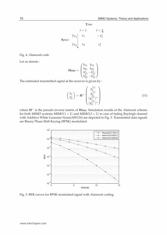
where H+ is the pseudo inverse matrix of Hequ. Simulation results of the Alamouti schemefor both MIMO systems MIMO(1 × 2) and MIMO(2 × 2) in case of fading Rayleigh channelwith Additive White Gaussian Noise(AWGN) are depicted in Fig. 5. Transmitted data signalsare Binary Phase Shift Keying (BPSK) modulated.

0 5 10 1510

−6

10−5

10−4

10−3

10−2

10−1

100

SNR(dB)

BE

R

RayleighTx1Rx1

AlamoutiTx2Rx1

AlamoutiTx2Rx2

Fig. 5. BER curves for BPSK modulated signal with Alamouti coding


www.intechopen.com

3.3 Frequency diversity

Frequency diversity relies on the fact that signals are transmitted on different frequenciesso that different multipath structures in the propagation media are exploited. Transmittingsignals on different frequencies are referred as multicarrier transmission. One special case ofmulticarrier transmission is Orthogonal Frequency Division Multiplexing (OFDM). OFDMhas got a great interest by the researchers and it was shown that using this type of modulationgives a significant performance increase in wireless communications. OFDM modulationtechnique was adopted by IEEE802.11a and IEEE 802.11b wireless LAN standards. Whenusing the OFDM technique, a single data stream is transmitted over a number of lowerrate carriers. This can be considered as a form of frequency multiplexing that could beefficient for wide band communication. The signal frequency band is divided into severalfrequency subchannels in order to get narrow band channels. Orthogonality between differentmodulated carriers is imposed in order to avoid overlapping subchannels. Therefore,signals are received without adjacent carrier interference. Both transmitter and receiver areimplemented using respectively the Inverse Fast Fourier Transform (IFFT) and Fast FourierTransform (FFT) techniques. The OFDM transmission scheme introduces guard bands /cyclicprefix between the different carriers. This lowers the spectrum efficiency but it eliminates theInter Symbol Interference (ISI). It should be noted that when using OFDM technique, channelequalization becomes simpler. Simulation of the OFDM system was performed in order tomeasure the performance of such technique and compare it to the single carrier system. Thesimulated OFDM system is given by Fig. 6.

S/P IFFT +CP P/S

S/P−CPFFTP/S

H

Modulated Input

Demodulated receive

......

...

......

......signal

signal

+b

Fig. 6. General structure of OFDM system

• P/S: Parallel to serial conversion

• S/P: Serial to parallel conversion

• +CP: Adding the cyclic prefix

• −CP: Removing the cyclic prefix

• H: Channel matrix

• b: Additive noise

For simulation, we consider a BPSK modulation scheme, a FFT length equal to 52 and a FFTsize of 64. The simulation results are given by Fig. 7. OFDM can be used in conjunction witha MIMO system. MIMO-OFDM (See Fig. 8) is interesting for high data rate systems. A designand simulation of MIMO-OFDM was introduced in (Yu et al., 2004).


www.intechopen.com

0 2 4 6 8 1010

−6

10−5

10−4

10−3

10−2

10−1

100

SNR(dB)

BE

R

OFDM

Theory BER

NoOFDM

Fig. 7. BER curve for BPSK modulated signal using OFDM in AWGN channel

Tx1Rx1

TxNT RxNR

Channel Receiver...

......

......

...

OFDM OFDM

OFDMOFDM

Modulator 1 Demodulator 1

Demodulator NRModulator NT

Data 1

Data NT

(IFFT + CP) (−CP + FFT)

Fig. 8. MIMO-OFDM system

3.4 Pattern diversity

Pattern diversity consists of the use of several colocated antennas with different radiationpatterns. This type of diversity can provide a higher gain versus a single omnidirectionalantenna if antennas are enough spaced and adequately polarized.

3.5 Polarization diversity

Polarization diversity is a diversity technique where different polarizations are used.Horizontal and vertical polarizations could be used so that to provide diversity. At the MIMOreceiver for example, the antennas take advantage of the multipath propagation characteristicsto receive separate uncorrelated signals.

4. MIMO channel modeling

4.1 Geometry-based Stochastic Channel Models (GSCM)

Geometry-based Stochastic Channel Models(GSCM) have an immediate relation to physicalreality. Such models are based on geometrical considerations, mainly scatterer locations andchannel impulse response behavior. We distinguish the Double Bounce Geometry-based


www.intechopen.com

Stochastic Channel Models (DB-GSCM) and the Single Bounce Geometry-based StochasticChannel Models (SB-GSCM).

4.1.1 Double Bounce Geometry-based Stochastic Channel Models (DB-GSCM)

Geometry based stochastic channel models represent the channel in a propagation-basedstochastic way in which the geometry is represented by statistical means. The GSCM isbased on the concept of clusters of scatterers around the transmitter and the receiver. Thescatterer locations are defined according to a random fashion that follows a particularprobability distribution. Scatterers represent discrete channel paths and can involve statisticalcharacterizations of several propagation parameters such as delay spread, angular spread,spatial correlation and cross polarization discrimination. These parameters will be detailedin the following sections. Fig. 9 shows a random geometrical two circle model in which thegeometry of the scatterers follows a circular distribution. Each propagation path is able to havetwo times of reflection by scatterers, one at transmitter side and another one at receiver side.Local scatterers around the transmit antennas and receive antennas are respectively situatedin a circle of radius RT and a circle of radius RR. The distance between the receive antennasand transmit antennas D is assumed to be longer than the radii RT and RR as depicted on Fig.9.

Tx1 Rx1

TxNTRxNR

......

Scatterers around the transmitter Scatterers around the receiver

D

RT RR

Fig. 9. Double Bounce Scattering Mechanism

4.1.2 Single Bounce Geometry-based Stochastic Channel Models (SB-GSCM)

When a single bounce of scatters is placed around the transmit antennas or the receiveantennas, this is referred as SB-GSCM. SB-GSCM models are originally considered in systemswhere the base station is elevated and there is no local scattering obstruct while the mobilestation (at the receive side) is surrounded by scatterers (Raoof & Zhou, 2009).

4.2 Stochastic channel models

Stochastic channel models can be split into three categories :

1. Correlation based models

2. Stochastic models of scatterers

3. Based propagation models

In the following, we briefly review the listed channel models.


www.intechopen.com

4.2.1 Correlation models

The independent and identically distributed (i.i.d) model

The listed models are normally calculated analytically. Hence, the channel matrix H can beexplicitly expressed. The simplest model is the i.i.d model. This supposes that multipathchannels in presence of scatterers are independent and uniformly distributed in all directions.The MIMO channel coefficients are statically independent with equal variance.

The Kronecker MIMO channel model

Kronecker model assumes that spatial transmit correlation and spatial receive correlation areseparable. Therefore, the full channel correlation matrix can be modeled by the Kroneckerproduct of the transmit and receive correlation matrix. Full channel correlation matrices isexpressed as :

Hcorr = RTx ⊗ RRx (12)

where :

• RTx= E[HHKronHKron] is the transmit correlation matrix.

• RRx= E[HKronHHKron] is the receive correlation matrix.

• ⊗ denotes the Kronecker product. The Kronecker product for matrices A and C is definedas :

A ⊗ C =

⎛

⎝

A11C A12C . . .A21C A22C . . .

. . . . . . . . .

⎞

⎠

The channel matrix according to the Kronecker model is expressed as (Biglieri et al., 2007):

HKron = R1/2Rx Hw(R1/2

Tx ) (13)

Hw is an i.i.d. Rayleigh fading channel. Note that there are others MIMO channel modelsbased on the Kronecker such as the Keyhole model and Weichselberger model. A review ofthese models is presented in (Raoof & Zhou, 2009).

4.2.2 Stochastic scatterer model

This section gives a generic description of stochastic models of scatterers. Multipath channelsare grouped into clusters according to statistical considerations. Besides, parameters for thechannel impulse response are determined in a random manner without referring to thegeometry of a physical medium. We mainly focus on the Saleh & Valenzuela (SVA) model(Saleh & Valenzuela, 1987). For finite numbers of clusters and multipath components, theimpulse response of the SVA channel model is expressed as :

h(t) =Lc

∑l=1

Km

∑k=1

αk,lexp(jΨk,l)δ(t − Tl − τk,l) (14)

where :

• Lc: Number of clusters which is Poisson distributed

• Km: Number of multipath propagation components which are grouped into a cluster

• αk,l : Tap weight of the k-th path component of the l-th cluster

• Ψk,l : The phase of the k-th path component of the l-th cluster


www.intechopen.com

• Tl : Delay of the l-th cluster

• τk,l : Delay of the k-th multipath component relative to the l-th cluster arrival time Tl

• δ(.) is the Dirac delta function

We assume that τk,l, k = 1, . . . , Km; l = 1, . . . , Lc are computed relatively to the firstpropagation component. Therefore, τ1,l = 0; l = 1, . . . , Lc. Both cluster delay and multipathcomponent delay are given by Poisson processes. The described model was also extendedto the spatial domain by including direction of departure and direction of arrival. Thenormalized directional channel impulse response can be written as :

h (t, φT, φR) = 1√LcKm

Lc

∑l=1

Km

∑k=1

αklexp(jΨk,l)δ(

t − Tl − τk,l

)

×δ(

φT − ΦT,l − φT,k,l

)

δ(

φR − ΦR,l − φR,k,l

)

(15)

here :

• Tl : Initial arrival time

• ΦT,l : Mean departure angle of the l-th cluster

• ΦR,l : Mean arrival angle of the l-th cluster

• τk,l : Initial arrival time with respect to the l-th cluster

• φT,k,l : Departure angle with respect to the initial time and mean angle of the l-th cluster

• φR,k,l: Arrival angle with respect to the initial time and mean angle of the l-th cluster

The parameters Lc and Km are important for channel modeling design. They respectivelydepend on two other parameters which are the cluster decay factor and the ray decayfactor. Fig. 10 shows the simulation results for the SVA model channel where four clustersof multipath components are obtained.

0 5 10 15 20 25 30 350

0.1

0.2

0.3

0.4

0.5

0.6

0.7

0.8

0.9

1

t(ns)

h(t

)

Cluster 1

Cluster 2

Cluster 3

Cluster 4

Fig. 10. Saleh & Valenzuela channel impulse response model for a SISO link


www.intechopen.com

4.2.3 Geometrical propagation model

Several existing analytic models are not coinciding with real situation. In fact, they rarelyconsider the effect of topology structure on radio channel propagation. Geometrical-basedpropagation model shows a more general model in which propagation considerations areinvolved. For seek of brevity, we consider the example of the finite scatterer model. Let usconsider the Uniform Linear Antenna (ULA) antennas at both the transmit and the receivesides. Assume that the element spacing between two close antennas at transmit and receivesides are respectively denoted by dT and dR. We consider finite number of scatterers that arelocated far away from the transmitter and the receiver. In the finite scatterer model, each pathspecifies a Direction of Departure (DOD) φT from the transmitting array and the Direction ofArrival (DOA) φR at the receiving array. According to these considerations, transmitting andreceiving steering vectors are expressed as (Burr, 2003):

aT (θT) = [1, exp −j2πθT , · · · , exp −j2π (NT − 1) θT]TaR (θR) = [1, exp −j2πθR , · · · , exp −j2π (NR − 1) θR]T

(16)

• θT = dT sin (φT) /λ

• θR = dR sin (φR) /λ

• λ is the wavelength of radio propagation.

The discrete channel model with Ls scatterers is therefore expressed via the array steering andresponse vectors as:

HS =Ls

∑l=1

βlaR

(

θR,l

)

aHT

(

θT,l

)

= AR (θR) HPAHT (θT) (17)

• βl is the complex amplitude of the l-th path

• HP = diag (β1, · · · , βLs)

• AT

(

θT,l

)

= [aT (θT,1) , · · · , aT (θT,Ls)]

• AR

(

θR,l

)

= [aR (θR,1) , · · · , aR (θR,Ls)]

5. Performance analysis of MIMO systems based on capacity

5.1 Some entropy terminologies (G.Proakis, 1995)

We briefly review in this paragraph some terminologies that we need for the channel capacityderivation.

Entropy: The entropy H(X) of a variable X measures the uncertainty about the realization ofX. Let X be a random variable with a probability function p(x) = PX = x, x = x1, . . . , xn

are possible values of X from a set of possible realizations χ. The entropy H(X) of thevariable X is expressed as :

H(X) = E[−log2(p(x))]

= − ∑x∈χ

p(x)log2(p(x)) (18)

E denotes the expected function.


www.intechopen.com

Joint entropy: The joint entropy measures how much information is contained in a jointsystem of two random variables. Given two random variables X and Y with respectiveprobability functions p(x) and p(y), the joint entropy is expressed as :

H(X, Y) = −∑x∈χ

∑y∈Y

p(x, y)log2(p(x, y)) (19)

Y denotes the set of possible values of y.

Conditional entropy : Suppose X and Y are random variables. Then, for any fixed value xof X, we get a conditional probability distribution on Y. We denote the associated randomvariable by H(Y|X). Conditional entropy is then :

H(Y|X) = H(X, Y) − H(X) (20)

Mutual information : Mutual information is a quantity that measures the dependencebetween two arbitrary random variables. The mutual information between two discreterandom variables X and Y is defined to be :

I(X, Y) = H(X) + H(Y)−H(X, Y)

= H(Y)−H(Y|X) (21)

5.2 Capacity definition based on information theory

Deterministic capacity

Channel capacity measures the maximum amount of information that could be transmittedthrough a channel and received with negligible error. Hence :

C = maxp(x)

I(X, Y) (22)

For a SISO link with input signal x, AWGN b and a constant channel gain h, the output signaly is expressed as :

y = hx + b (23)

The mutual information is expressed as :

I(x, y) = H(y)−H(b)

≤ log2(πe(PT + σ2b )) − log2(πeσ2

b )

= log2

(

1 +PT

σ2b

)

where :

• PT = E|x|2 is the transmit power

• σ2b = E|b|2 is the noise power

• log(e) = 1

Finally, the normalized channel capacity is given by :

CSISO = log2

(

1 +PT

σ2b

)

bits/s/Hz (24)

This is referred as the famous Shannon’s channel capacity.


www.intechopen.com

Ergodic capacity

In information-theoretical sense, ergodic capacity refers to the maximum rate thatcommunication can be achieved; assuming that the communication duration is long enoughto exploit all channel state. In fact, the propagation channel varies in time. This causes thechannel capacity varying in time. Consequently, to measure the fluctuating channel capacityin information theory, ergodic capacity is defined. Ergodic capacity refers to the maximumrate that can be achieved during a long observation communication to exploit all channelinformation. Ergodic capacity CSISO is an expected value. For a SISO channel h, CSISO isderived as :

CSISO = E

maxp(x):E|x|2PT

I(x, y)

bits/s/Hz (25)

which could be also expressed as :

CSISO = E

log2(1 +PT

σ2b

|h|2)

bits/s/Hz (26)

Outage capacity

Outage capacity is an another statical parameter on which relies the channel performance.Outage capacity is defined as the probability that the capacity C(h) is lower than a certainthreshold Cout. Outage capacity is expressed as :

Pout = Pr (C(h) < Cout) (27)

Outage probability is related to the Complementary Cumulative Distribution Function(CCDF):

CCDF = 1 − Pout (28)

In the following, we consider a MIMO system with NT transmit antennas and NR receiveantennas. We assume that the channel is flat fading. The received signal at antenna q, yq isexpressed as :

yq =NT

∑p=1

hqpxp + bq ; q = 1, . . . , NR (29)

The MIMO channel capacity is derived as :

I(x, y) = H(y)−H(y|x) (30)

H(y) and H(y|x) are respectively the received signal entropy and the entropy of y|x. Asthe received signal y and the signal noise b are independents, H(y|x) = H(b). Thereafter,the capacity is obtained by maximizing the received signal entropy. For MIMO capacityderivation, we denote :

• Rx = E

xxH

: Covariance matrix of the transmit signal

• Rb = E

bbH

: Covariance matrix of the noise signal

• Ry = E

yyH

: Covariance matrix of the received signal


www.intechopen.com

Thus :Ry = HRxHH + Rb (31)

The mutual information is expressed as :

I(x, y|H) = log2 det(

πeRy)

− log2 det (πeRb)

= log2 det

INR+ HRxHH(Rb)−1

(32)

For circularly symmetric Gaussian random vectors, the mutual information is maximum andalso expressed as :

CMIMO = maxp(x):ExHx≤PT

I(x, y|H) bits/s/Hz (33)

When no CSI (Channel State Information) is available at the transmitter, equal powerallocation is adopted. With the assumption that no correlation exits at the transmit side,

Rx =PT

NTINT

PT is the total power available at the transmit side.The MIMO capacity is then expressed as :

CMIMO = log2 det

(

INR+

γ

NTHHH

)

bits/s/Hz (34)

γ is the SNR.

5.3 MIMO capacity based on SVD: CSI known at the receiver

When CSI is available at the receiver, SVD factorization is used and MIMO channel capacitycould be easily derived. Let us first review the SVD technique. SVD is a factorization methodfor complex matrix which is widely used in signal processing. We take an (N × M) matrix A,SVD theorem states:

A = USVH (35)

• The eigenvectors of AAH make up the columns of U(N × N) which is an unitary matrix(UUH = IN).

• The singular values in S(N × M) are square roots of eigenvalues from AAH or AHA. Thesingular values are the diagonal entries of the S matrix and are arranged in descendingorder.

• The eigenvectors of AHA make up the columns of V. V(M × M) is also a unitary matrix(VVH = IM).

Calculating the SVD of the MIMO channel matrix H leads to the following factorization :

H = USVH (36)

We substitute H by its SVD decomposition. Hence, the received signal is expressed as :

y = USVHx + b (37)


www.intechopen.com

Let :

y′= UHy

x′= VHx

b′= UHb (38)

As U and V are unitary matrix, variables x′

and b′

keep the same statistical densities as x andb. Therefore, the channel model (y = Hx + b) could be also presented as :

y′= Sx

′+ b

′(39)

• y′= [y

′1, . . . , y

′NR

]T

• x′= [x

′1, . . . , x

′NT

]T

• S=diag(√

λ1, . . . ,√

λR, 0, . . . , 0) ; R = min(NR, NT) is the rank of the channel matrix H.

Equation (1) can be rewritten as:

y′i =

√λix

′i + b

′i, i=1,. . . ,R;

b′i, i=R+1,. . . ,NR.

(40)

According to the equation above, the MIMO channel consists of R uncorrelated subchannels.

The covariance matrix of the signals y′, x

′and b

′are expressed as :

Ry′y′ = UHRyyU

Rx′x′ = VHRxxV

Rb′b′ = UHRbbU (41)

and

tr(Ry′ y′ ) = tr(Ryy)

tr(Rx′x′ ) = tr(Rxx)

tr(Rb′b′ ) = tr(Rbb) (42)

The capacity of the MIMO channel is the summation of the R uncorrelated subchannels.Hence:

CSVD =R

∑i=1

log2

(

1 +γ · λi

NT

)

= log2

R

∏i=1

(

1 +γ · λi

NT

)

; γ =PT

σ2b

bits/s/Hz (43)

One eigenvalue λ of HHH is obtained according to the following equation :

(λIR − Q)y = 0 ; y = 0 (44)


www.intechopen.com

Q is the Wishart matrix :

Q =

HHH , NR < NT;

HHH, NR ≥ NT.(45)

λ is an eigenvalue of the matrix channel H. Hence :

det(λIR − Q) = 0

The associate characteristic polynomial of the channel matrix is the polynomial defined by :

p(λ) = det(λIR − Q)

which is also expressed as :

p(λ) =R

∏i=1

(λ − λi) (46)

If we substitute λ by (−NTσ2

bPT

) then :

R

∏i=1

(1 +γ · λi

NT) = det

(

IR +fl

NTQ

)

; γ =PT

σ2b

(47)

If NR < NT then equation (43) becomes :

CSVD = log2 det

(

IR +γ

NTHHH

)

bits/s/Hz (48)

Finally,

CSVD = R · log2 det

(

1 +γ

NTHHH

)

bits/s/Hz (49)

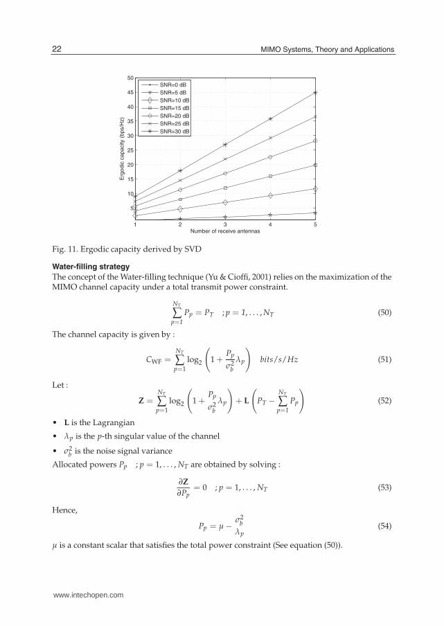
Simulation results for the ergodic MIMO capacity when CSI is available at the receiver isdepicted in the Fig. 11. For a MIMO system with two transmit antennas, ergodic capacityincreases linearly with the number of antennas. Ergodic capacity depends on the SNR level.Plotted curves show that capacity grows with the SNR.

5.4 MIMO capacity based on Water-filling technique : CSI known at both transmitting and

receiving sides

When CSI is available at both the transmitter and the receiver, an optimal power allocationcould be exploited. This is referred as the water-filling technique. The main idea ofwater-filling strategy is to allocate more power to better subchannels with higher SNR so asto maximize the sum of data rates in all subchannels where in each subchannel the data rateis related to the power allocation by Shannon’s Gaussian capacity formula 1

2 log2(1 + SNR).


www.intechopen.com

1 2 3 4 5

5

10

15

20

25

30

35

40

45

50

Number of receive antennas

Erg

odic

capacity (

bps/H

z)

SNR=0 dB

SNR=5 dB

SNR=10 dB

SNR=15 dB

SNR=20 dB

SNR=25 dB

SNR=30 dB

Fig. 11. Ergodic capacity derived by SVD

Water-filling strategy

The concept of the Water-filling technique (Yu & Cioffi, 2001) relies on the maximization of theMIMO channel capacity under a total transmit power constraint.

NT

∑p=1

Pp = PT ; p = 1, . . . , NT (50)

The channel capacity is given by :

CWF =NT

∑p=1

log2

(

1 +Pp

σ2b

λp

)

bits/s/Hz (51)

Let :

Z =NT

∑p=1

log2

(

1 +Pp

σ2b

λp

)

+ L

(

PT −NT

∑p=1

Pp

)

(52)

• L is the Lagrangian

• λp is the p-th singular value of the channel

• σ2b is the noise signal variance

Allocated powers Pp ; p = 1, . . . , NT are obtained by solving :

∂Z

∂Pp= 0 ; p = 1, . . . , NT (53)

Hence,

Pp = μ − σ2b

λp(54)

μ is a constant scalar that satisfies the total power constraint (See equation (50)).


www.intechopen.com

Capacity calculation based on Water-filling

Let R be the rank of H. The allocated power for the subchannel p is expressed as :

Pp =

(

μ − σ2b

λp

)+

; p = 1, . . . , R (55)

where :a+ = max(a, 0)

The received power at the subchannel p is then :

Prp =(

λpμ − σ2b

)+(56)

Hence, the channel capacity is expressed as :

CWF = ∑p

log2

(

1 +Prp

σ2b

)

bits/s/Hz (57)

Finally, the channel capacity is :

CWF =R

∑p=1

log2

⎡

⎣

(

λpμ

σ2b

)+⎤

⎦ bits/s/Hz (58)

Some numerical results for Water-Filling technique

We present some numerical results in order to simulate the performance of the water-fillingtechnique. Let us consider a correlated MIMO(4 × 4) channel that follows the Kroneckermodel. We simulate the ergodic capacity according to both cases:

1. Equal power allocation for the transmit antennas

2. Optimal power allocation with Water-filling (WF) algorithm

Simulation results are depicted in Fig. 12. The MIMO capacity is improved by optimalpower allocation strategy but stills affected by channel correlation. Simulation of the CCDF isshown in Fig. 13. The CCDF is improved by exploiting the WF technique for optimal powerallocation. We present simulation results for the CCDF for two SNR values: SNR = 6dB andSNR = 10dB.

Water-filling technique: discussion

Water-filling provides an optimal power allocation and is an attractive strategy for capacityimprovement. Nevertheless, capacity gain appears significant when more transmit antennasthen receive antennas are deployed, i.e NR ≤ NT. Moreover, this gain is considerable forlow SNRs and is specially interesting in the case of correlated channels. Fig. 14 shows thatthe capacity gain is negligible for low SNRs and is almost null for high SNR values. CCDFsfor the MIMO(4 × 2) are depicted in Fig.15 and Fig. 16 respectively for high SNR value thatis equal to 18 dB and low SNR of 2 dB. Simulation results confirm that WF technique bringsmore performances for high noise strength and correlated MIMO channel. Finally, at high SNRvalue, the WF gain in ergodic capacity for MIMO(NR × NT) is expressed as (Prayongpun,2009):

CWF − CMIMO =

0 if NT ≤ NR

R log2

(

NTR

)

if NT > NR(59)

where R = min(NR, NT).


www.intechopen.com

0 5 10 15 200

5

10

15

20

25

SNR (dB)

MIM

O C

apacity (

bits/s

/Hz)

Uniform power allocation

Optimal power allocation

Optimal power allocation (Uncorrelated MIMO channel)

Fig. 12. MIMO(4 × 4): Capacity improvement with WF strategy-Channel correlation impacton system capacity

2 4 6 8 10 12 140

0.1

0.2

0.3

0.4

0.5

0.6

0.7

0.8

0.9

1

Capacity(bits/s/Hz)

P(C

> a

bscis

se)

NoWF−SNR=6dB

NoWF−SNR=10dB

WF−SNR=6dB

WF−SNR=10dB

SNR=6dB

SNR=10dB

Fig. 13. CCDF for MIMO(4 × 4) with various SNR values


www.intechopen.com

0 5 10 15 202

4

6

8

10

12

14

SNR (dB)

MIM

O C

apacity (

bits/s

/Hz)

No WF

WF

Fig. 14. Ergodic capacity for MIMO(4 × 2)-Kronecker channel model

4 5 6 7 8 9 10 11 120

0.1

0.2

0.3

0.4

0.5

0.6

0.7

0.8

0.9

1

Capacity (bits/s/Hz)

P(C

> a

bscis

se)

NoWF

WF

Fig. 15. CCDF for MIMO(4 × 2)-Kronecker channel model (SNR=18dB)


www.intechopen.com

0.5 1 1.5 2 2.5 3 3.5 4 4.5 5 5.50

0.1

0.2

0.3

0.4

0.5

0.6

0.7

0.8

0.9

1


P(C

>abscis

se)

NoWF

WF

Fig. 16. CCDF for MIMO(4 × 2)-Kronecker channel model (SNR=2dB)

6. Combining techniques for MIMO systems

MIMO system can use several techniques at the receiver so that to combine the multipleincoming signals for more robust reception. Combining techniques are listed below :

1. Maximal Ratio Combining (MRC): Incoming signals are combined proportional to the SNRof that path signal. The MRC coefficients correspond to the relative amplitudes of the pulsereplicas received by each antenna such that more emphasis is placed on stronger multipathcomponents and less on weaker ones.

2. Equal Gain Combining (EGC) simply adds the path signals after they have been cophased(Sanayei & Nosratinia, 2004).

3. Selection Combining (SC) selects the highest strength of incoming signals from one of thereceiving antennas.

Combining techniques can be carried so that to satisfy one or more targets :

1. Maximizing the diversity gain

2. Maximizing the multiplexing gain

3. Achieving a compromise between diversity gain and multiplexing gain

4. Achieving best performances in terms of Bit Error Rate (BER)

5. Maximizing the Frobenius norm of the MIMO channel and therefore the MIMO channelcapacity

Let us recall the SIMO system model with NR receive antennas. The received signal at the q-threceive antenna is expressed as :

yq = hqx + bq ; q = 1, . . . , NR (60)

hq is the q-th complex channel gain, bq is an AWGN with zero mean and variance σ2b .

We keep for notations :


www.intechopen.com

• PT: Transmit signal power

• γ = PT

σ2b

is the SNR

We assume channel normalization and a perfect channel estimation. We will be moreinterested in the combining module. Our aim is to derive the combining coefficients gq ; q =1, . . . , NR. The output signal at the combining module can be expressed as:

y = xNR

∑q=1

gqhq +NR

∑q=1

gqbq (61)

Combining technique in MIMO system is depicted in Fig.17. Combining coefficients relativeto the listed techniques are given by:

Combining technique Combining coefficient

MRC gq = h∗qEGC gq =

h∗q

|hq|

SC gq =

1,∣

∣hq

∣

∣ |hk| , ∀k = q;0, otherwise.

Table 1. Combining coefficients

Rx1

RxNR

RxqTxp

x

⊕

⊕

⊕

⊗

⊗

⊗

b1

bNR

bq

g1

gNR

gq

∑ y

...

...

...

...

...

...

⑦

Fig. 17. SIMO system with combining technique

6.1 Maximal Ratio Combining (MRC)

The equivalent SNR of MRC has been calculated as :

γy = γ ·

(

NR

∑q=1

∣

∣hq

∣

∣

2

)2

NR

∑q=1

∣

∣hq

∣

∣

2= γ ·

NR

∑q=1

∣

∣hq

∣

∣

2=

NR

∑q=1

γq (62)

Thus, the instantaneous SNR γy is expressed as the sum of the instantaneous SNR at differentreceive antennas. For normalized channel matrix, the SNR is then:

γy = NR · γ (63)


www.intechopen.com

The system capacity with MRC is :

CMRC = log2

(

1 + γ ·NR

∑q=1

∣

∣hq

∣

∣

2

)

bits/s/Hz (64)

6.2 Equal Gain Combining (EGC)

The instantaneous SNR is expressed as :

γy =γ

NR·(

NR

∑q=1

|hq|)2

(65)

Resulting capacity has been calculated as :

CEGC = log2

(

1 +γ

NR·

NR

∑q=1

∣

∣hq

∣

∣

2

)

bits/s/Hz (66)

6.3 Selection Combining(SC)

The receiver scans the antennas, finds the antenna with the highest instantaneous SNR andselects it. We denote the highest received instantaneous SNR as :

γy = max (γ1, . . . , γNR) (67)

The SNR at the output of the combiner for an uncorrelated channel is:

γy = γ ·NR

∑q=1

1

q(68)

SC capacity is expressed as:

CSC = log2

(

1 + γ · maxq

∣

∣hq

∣

∣

2)

= maxq

log2

(

1 + γ ·∣

∣hq

∣

∣

2)

; 1 ≤ q ≤ NR bits/s/Hz (69)

The ergodic capacity curves for all three combining strategies are shown in Fig. 18. MRC yieldsbest performances in terms of channel capacity. However, MRC is the optimal combiningtechnique, MRC is seldom implemented in a multipath fading channel since the complexityof the receiver is directly resolvable paths (Zhou & Okamoto, 2004). In general, EGC performsworse than does MRC. Obviously, lower capacity is obtained with SC since only one RadioFrequency (RF) channel is selected at the receiver. A study of combining techniques interms of BER was presented in (Zhou & Okamoto, 2004). MRC steel achieves the best BERperformances.

7. Beamforming processing in MIMO systems

Beamforming is the process of trying to steer the digital baseband signals to one particulardirection by weighting these signals differently. This is named "digital beamforming" andwe call it beamforming for the sake of brevity, (Jafarkhani, 2005). The desired signal is thenobtained by summing the weighted baseband signals.


www.intechopen.com

0 1 2 3 4 5 6 7 810

−7

10−6

10−5

10−4

10−3

10−2

10−1

SNR(dB)

BE

R

LR

=1

LR

=3

LR

=4

Fig. 18. Capacity for MIMO(4 × 1) using various combining techniques-Rayleigh fadingchannel

7.1 Beamforming based on SVD decomposition

In this section, we provide an overview of MIMO systems that use beamforming at boththe ends of the communication link. We consider a MIMO system with NT transmitand NR receive dimensions. From a mathematical point of view, joint Transmit-Receivebeamforming is based on the minimization (or maximization) of some cost function such asSNR maximization. This method includes determining the transmit beamforming coefficientsand the receive beamforming coefficients so that to steer relatively all transmit energy andreceive energy in the directions of interest. Joint Transmit-Receive beamforming is illustratedin Fig. 19.

Rx1Tx1

RxNRTxNT

RxqTxp

⊕⊗

⊕⊗

⊕⊗

⊗

⊗

⊗

b1Wt1

bNRWtNT

bqWtp

Wr1

WrNR

Wrq

∑yBF

......

......

......

......

...

...

x

Fig. 19. Joint Transmit-Receive beamforming

• x: The transmit signal

• Wt = [Wt1,. . .,WtNT]T : The (NT × 1) Transmit beamforming vector


www.intechopen.com

• H: The (NR × NT) channel matrix

• Wr = [Wr1,. . .,WrNR]T : The (NR × 1) Receive beamforming vector

• b = [b1, . . . , bNR]T : The (NR × 1) Additive noise vector with variance σ2

b

• yBF: The output signal

Joint Transmit-Receive beamforming can be described by equation (70).

yBF = WrHHWt · x + WrH · b (70)

Eigen-beamforming could be performed by using eigenvectors to find the linear beamformerthat optimizes the system performances. Thus, we exploit the SVD factorization for channelmatrix H (H = USVH). Assigning U and V respectively to Wr and Wt is optimal formaximizing the SNR given by :

SNRBF =‖WrHHWt‖2E(xxH)

σ2b ‖Wr‖2

When SVD factorization is applied to MIMO channel matrix, equation (70) becomes :

yBF = S · x + UH · b (71)

Note that Beamforming (Ibnkahla, 2009) is considered as a form of linear combiningtechniques which are intended to maximize the spectral efficiency. The received SNR forcommunication system with beamforming is expressed as :

γBF = γr · λmax(H)

λmax is the maximum eigenvalue associated to matrix S and γr is the mean received SNR.Thereafter, the capacity for MIMO system with beamforming is expressed as :

CBF = log2 1 + γr · λmax(H) bits/s/Hz (72)

Simulation results for MIMO capacity where beamforming technique is performed are shownin Fig. 20. The MIMO channel capacity with beamforming is improved thanks to the spatialdiversity.Note that beamforming technique is shown to improve the performance of the communicationlink in terms of BER. Fig. 21 shows the plotted curves of BER as a function of SNR relative tothree cases :

• System performing beamforming

• Transmission without applying beamforming

• Transmission with simply Zero Forcing (ZF) equalization

The MIMO (3 × 3) channel is randomly generated and input signal is BPSK modulated. Weadopt the correlated MIMO channel with a spreading angle of 90 and an antenna spacing ofλ2 . Fig. 21 shows that associated SVD beamforming technique brings the best performances interms of BER.


www.intechopen.com

0 5 10 15 201

2

3

4

5

6

7

8

9

10

11

SNR(dB)

Capacity(b

its/s

/Hz)

SISO

MIMO(2X2)

MIMO(3X3)

MIMO(4X4)

Fig. 20. Capacity of MIMO system with beamforming technique

0 2 4 6 8 1010

−3

10−2

10−1

100

SNR (dB)

BE

R

BF

NoBF

ZF

Fig. 21. SVD based beamforming technique


www.intechopen.com

7.2 SINR maximization beamforming

Interference often occurs in wireless propagation environment. When several terminals aredensely deployed in the coverage area, Signal to Interference Noise Ratio (SINR) grows upand efficient techniques are required to be implemented. Beamforming is an efficient strategythat could be exploited so that to mitigate interference. Maximizing the SINR criteria could bealso considered so that to obtain optimal beamforming weights.

SINR maximization based beamforming in Multi user system

Model description

Rx1

Tx1

Rx1

RxM1

TxN

RxMK

...

...

...

...

UK

U1

BS

③

⑦

HK

H1♥+❫

♠

♠×

×

Wt1

WtK

e1

eK

...

e1

eK

...

Fig. 22. Multi user system with beamforming

We denote :

• K: Number of users.

• E = [e1, . . . , eN]T: The transmit signal vector

• Wt=[Wt1,. . .,WtK]T: Weight vector for beamforming

• M1, . . . , MK number of antennas respectively for users U1, . . . , UK

• x: The transmit vector signal of size (N × 1)

Transmit signal is expressed as :

x =K

∑k=1

Wtk · ek (73)

We assume that transmit signals and beamforming weights are normalized. The receivedsignal (Of size (Mi × 1)) by user Ui is :

yi = Hi

K

∑k=1

Wtk · ek + bi (74)


www.intechopen.com

bi is the additive noise with variance σ2i . The channel matrix Hi(Mi × N) between user Ui with

Mi antennas and the N antennas at the Base Station (BS) is assumed to be normalized. UserUi ; i = 1, . . . , K receives the signal :

yi = HiWti · ei +K

∑k=1,k =i

HiWtk · ek + bi (75)

At the receiver, the estimated signal for user i is:

ei =WtH

i HHi yi

‖HiWti‖(76)

The SINR is the ratio of the received strength of the desired signal to the received strength ofundesired signals (Noise + Interference). Associated SINR to user i is expressed as :

SINRi =‖ HiWti ‖2

(

K∑

k=1,k =i‖ HiWtk ‖2

)

+ σ2i

(77)

SINR could also be written as :

SINRi =‖ HiWti ‖2

⎛

⎜

⎝

K

∑k=1,k =i

‖WtHi HH

i HiWtk‖2

‖HiWti‖2

⎞

⎟

⎠+ σ2

i

(78)

Optimal beamformer weights are obtained by maximizing the Signal Leakage Ratio (SLR)metric expressed as :

SLR =‖ HiWti ‖2

‖ HiWti ‖2(79)

where :

Hi = [HH1 , . . . , HH

i−1, HHi+1, . . . , HH

K ]H (80)

The optimal weights Wti ; i = 1, . . . , K are derived (Tarighat et al., 2005) as the maximumeigenvector of:

((HiH

Hi)−1(HH

i Hi))

Simulation results are shown in Fig. 23. These results show that the method is optimal fordetermining the beamforming weights. Note that better performances in terms of BER areachieved if more transmit antennas are used.


www.intechopen.com

0 1 2 3 4 5 6 7 810

−4

10−3

10−2

10−1

SNR(dB)

BE

R

M=4

M=3

Fig. 23. Multi user BF (K = 3, M = 3/M = 4)

8. Processing techniques for MIMO systems: Antenna selection

MIMO system gives high performances in terms of system capacity and reliability ofradio communication. Combining techniques such as MRC results in more robust system.Nevertheless, the deployment of multiple antennas would require the implementation ofmultiple RF chains (Dong et al., 2008). This would be costly in terms of size, power andhardware. For example, when several antennas are deployed, multiple RF chains withseparate modulator and demodulator have to be implemented. To overcome these limitations,antenna selection techniques can be applied.

8.1 Antenna selection

Antenna selection technique (Ben ZID et al., 2011) is depicted in Fig. 24. We consider a MIMOsystem with NT transmit antennas and NR receive antennas. The idea of antenna selection isto select LT antennas among the NT transmit antennas and / or LR antennas among the NR

receive antennas. We distinguish different forms of antenna selection:

1. Transmit antenna selection

2. Receive antenna selection

3. Hybrid antenna selection: that is when antenna selection is carried among both transmitantennas and receive antennas.

Tx Rx

Tx1 Rx1

TxNTRxNR

......

...

......

...

RF

RF

RF

RF

Chain

Chain Chain

Chain

1

LT LR

1

Fig. 24. Antenna selection in MIMO system


www.intechopen.com

Antenna selection algorithms do not only aim to reduce the system complexity but also toachieve high spectral efficiency. When LT antennas are selected at the transmitter and LR

antennas are selected at the receiver, the associated channel will be denoted HS. The capacityof such system is expressed as :

CSel = log2

[

det

(

ILT+

γ

LRHH

S HS

)]

= log2

[

det

(

ILR+

γ

LTHSHH

S

)]

(81)

γ denotes the SNR. The antenna selection algorithm is intended to find the optimal subsetof the transmit antennas and /or the optimal subset of the receive antennas that satisfycapacity system maximization. Nevertheless, it is obvious that the joint antenna selectionat the transmitter and the receiver brings more complexity when the number of antennasincreases.

Numerical results

Ergodic capacity of MIMO system with antenna selection at the transmitter and the receiveris shown in Fig. 25. For simulation purposes, we generate a Rayleigh MIMO channel withAWGN. Here, SVD factorization is applied. Plotted curves depict the ergodic capacity for theMIMO(4 × 4). This evidently leads to the highest system capacity. When 3 transmit antennasare selected among 4 transmit antennas and 3 receive antennas are selected among 4 receiveantennas, the maximum ergodic capacity that could be achieved is plotted in function of SNR.Simulation results are also presented in the case when two antennas are selected at both thetransmitter and the receiver. According to the plotted curves in Fig. 25, it is obvious that one ofthe important limitations of the antenna selection strategy is the important losses in capacityat high SNR regime.

0 5 10 15 205

10

15

20

25

30

35

SNR(dB)

Erg

odic

capacity

AS (2 Among 4)

AS (3 Among 4)

No AS

Fig. 25. Antenna selection in MIMO (4 × 2): Impact on ergodic capacity


www.intechopen.com

8.2 Antenna selection involving ST coding

We present in this paragraph, the simulation results in terms of average BER when jointAlamouti scheme and antenna selection at the receiver are applied. The MIMO (4× 2) systemwith a Rayleigh channel and AWGN was created. Emitted symbols are QAM (QuadratureAmplitude Modulation) modulated. The simulation model is given by the Fig. 26 (b1, . . . , bNR

denote the additive noise signals). Plotted curves concern subsets of receive antennas whereLR = 1 and LR = 3. Simulation results show that even with only one selected antenna at the

Rx1

RxNR

Rxq

Tx1

TxNT

⊕

⊕

⊕

b1

bNR

bq

...

...

...

...

⑦

1

LR

...

ST

decoderAlamoutiencoder

Antenna

selectionInput Output

Sequence Sequence

Fig. 26. MIMO system with antenna selection and Alamouti coding

0 1 2 3 4 5 6 7 810

−7

10−6

10−5

10−4

10−3

10−2

10−1

SNR(dB)

BE

R

LR

=1

LR

=3

LR

=4

Fig. 27. Joint Alamouti coding and antenna selection in MIMO (4 × 2)

receiver, performances in terms of BER still satisfactory. Nevertheless, when more antennasare selected, better BER values are achieved thanks to receive diversity.


www.intechopen.com

TxRx

②①②

②③ ③ΔR

Scatterers

Fig. 28. Angle spread

8.3 Antenna selection in correlated MIMO channel: Angular dispersion and channel

correlation

Angle spread refers to the spread of DOA of the multipath components at the transmit antennaarray. When scatterers are also distributed around the receive antennas, the scattering effectleads also to an angle spreading relative to the DOA. In Fig. 28, the angle spread is denoted ΔR.We present a SISO model rich of local scatterers. For seek of simplicity, we consider a MIMO(NR × NT) system with LOS channel and uniform antenna arrays at both the transmitter andthe receiver.We denote :

• H: MIMO channel matrix

• dq,p: distance between antenna q and antenna p

• ρq,q′ : correlation coefficient

• λ: wavelength

• R = E[HHH] Correlation matrix

• α: Angle of arrival

• p(α) : Probability density function of the DOA

• ΔR(= 2π): Angle spread at the receiving side

When LOS propagation is assumed, the channel coefficients can be expressed as :

hqp = e−j2πdq,p

λ ; q = 1, . . . , NR, p = 1, . . . , NT (82)

The correlation coefficient at the receiving side between two receive antennas of indexes q and

q′

is expressed :

ρq,q′ = E[exp(−j2πdq,q′ sinα

λ)] (83)

Formula for correlation coefficients is expressed as :

ρq,q′ =∫

ΔR2

−ΔR2

exp(−j2πdq,q′ sin(α)

λ)p(α)dα ; q = q

′(84)

Evidently :

ρq,q′ = 1 ; q = q′

(85)


www.intechopen.com

Following a uniform distribution, correlation coefficients can be expressed as :

ρq,q′ = J0(2πdq, q

′

λ) q = 1, . . . , NR; q

′= 1, . . . , NR (86)

J0(.) is the zeroth order Bessel function. When antennas are uncorrelated, ρq,q′ = 0 if q = q′.

Which induces :

J0(2πdq,q′

λ) ≃ 0 ⇒ 2π

dq,q′

λ≃ π

Thus, in order to mitigate correlation between antennas, antenna spacing between two

antennas should be at least equal to λ2 . Nevertheless, antenna correlation still depends on

angular dispersion. Fig. 29 presents the plotted curves of the spatial correlation as a function ofthe antenna spacing divided by the wavelength for various values of angle spread. Accordingto simulation results depicted in Fig. 29, we conclude that spatial correlation between twoantennas depends on antenna spacing and is reduced by higher angle spread.

0 1 2 3 4 50

0.1

0.2

0.3

0.4

0.5

0.6

0.7

0.8

0.9

1

d/λ

Sp

atia

l co

rre

latio

n

AS=10°

AS=30°

AS=90°

Fig. 29. Impact of angle spread on spatial correlation

Better performances in terms of BER are achieved for AS = 30 . This is due to the fact that fora given antenna spacing, system correlation is higher for lower angular spread. The impact ofangle spread on system performances is depicted in Fig. 30.

9. Multi polarization techniques

9.1 Basic antenna theory and concepts

We present in this paragraph, some basic concepts related to antenna. A rigorous analysis ofthe antenna theory and the related concepts is available in (Constantine, 2005). Antenna is atransducer for radiating or receiving radio waves. It ideally radiates all the power deliveredto it from the transmitter in a desired direction. The far electric field of the electromagneticwave is written in spherical coordinates as :

E = Eθ(θ, φ)θ + Eφ(θ, φ)φ (87)


www.intechopen.com

0.1 0.4 0.7 110

−6

10−5

10−4

10−3

d/λ

BE

R

AS=10°

AS=30°

Fig. 30. Impact of angle spread on system performances

Eθ and Eφ are the electric field components. θ and φ denote respectively the elevation angleand the azimuthal angle. We distinguish two categories of antennas :

1. Omnidirectional antenna is an antenna system which radiates power uniformly

2. Dipole antenna radiates power in a particular direction.

Electric dipole could be oriented along the x-axis, y-axis or the z-axis. Table 2 gives theexpressions of the electric field components relative to each antenna orientation.

Eθ(θ, φ) Eφ(θ, φ)x − cos(θ) cos(φ) sin(φ)y − cos(θ) sin(φ) − cos(φ)z sin(θ) 0

Table 2. Radiation pattern for electric dipole

Radiation intensity

Antenna gain is defined as the ratio of the intensity radiated by the antenna divided by theintensity radiated by an isotropic antenna. Normalized radiation intensity (or Antenna gain)is :

G (θ, φ) =

[

Gθ (θ, φ)Gφ (θ, φ)

]

=

⎡

⎢

⎢

⎢

⎢

⎢

⎢

⎢

⎢

⎢

⎢

⎢

⎢

⎣

Eθ (θ, φ)√

√

√

√

√

1

4π

⎛

⎝

2π∫

0

π∫

0

|Eθ (θ, φ) |2dΩ +

2π∫

0

π∫

0

|Eφ (θ, φ) |2dΩ

⎞

⎠

Eφ (θ, φ)√

√

√

√

√

1

4π

⎛

⎝

2π∫

0

π∫

0

|Eθ (θ, φ) |2dΩ +

2π∫

0

π∫

0

|Eφ (θ, φ) |2dΩ

⎞

⎠

⎤

⎥

⎥

⎥

⎥

⎥

⎥

⎥

⎥

⎥

⎥

⎥

⎥

⎦

(88)


www.intechopen.com

• Ω is the beam solid angle through which all the power of the antenna would flow if itsradiation intensity is constant for all angles within Ω.

• Gθ (θ, φ) and Gφ (θ, φ) are respectively the elevation antenna gain and the azimuthalantenna gain.

9.2 3D Geometric wide band channel model

The 3D Geometric wide band channel model is presented in Fig.31.

z z′

x x′

RxTx

A(1)Tx

A(2)Tx

A(1)Rx

A(2)Rx

R(ℓ)Tx D

(ℓ)Rx

CRx(ℓ)CTx(ℓ)S

(ℓ,n)Rx

S(ℓ,m)Tx

R(ℓ)Rx

D(ℓ)Tx

vRx

vTx

αRx

αTx

❲

θ(ℓ,m)Tx

θ(ℓ,n)Rx

y

Fig. 31. 3D Geometric model for MIMO channel (NR = 2, NT = 2)

Two transmit antennas (A(1)Tx ,A

(2)Tx ) and two receive antennas (A

(1)Rx ,A

(2)Rx ) are presented. Wide

band MIMO channel involves several local clusters of scatterers which are distributed aroundthe transmitter and the receiver. The cluster index is denoted ℓ, ℓ = 1, . . . , L. Cluster around

the transmitter CTx(ℓ) is assumed to be associated with a set of M(ℓ) scatterers (S(ℓ,m)Tx ; m =

1, . . . , M(ℓ)). Cluster around the receiver CRx(ℓ) is assumed to be associated with a set of N(ℓ)

scatterers (S(ℓ,n)Rx ; n = 1, . . . , N(ℓ)).

We take for notations:

• R(ℓ)Tx : Transmit cluster radius of index ℓ

• D(ℓ)Tx : Distance between the reference transmit antenna and the transmit cluster center

• d1,ℓ,m: Distance between antenna A(1)Tx and a scatterer S

(ℓ,m)Tx

• d2,ℓ,m: Distance between antenna A(2)Tx and a scatterer S

(ℓ,m)Tx

• dTx: Transmit antennas spacing

• DTx↔Rx: Distance between the transmitter and the receiver

• R(ℓ)Rx : Cluster radius at the receiver of index ℓ


www.intechopen.com

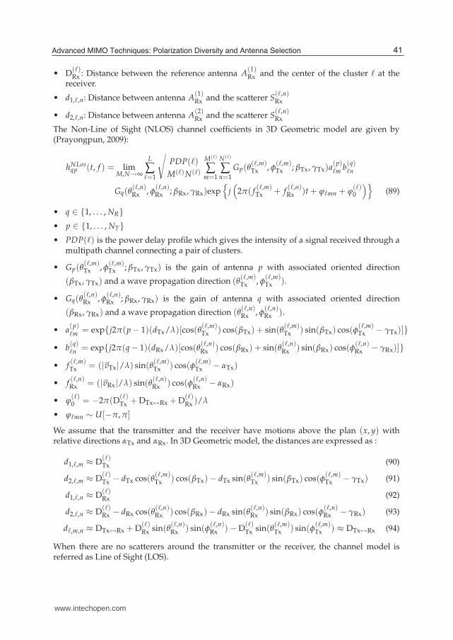
• D(ℓ)Rx : Distance between the reference antenna A

(1)Rx and the center of the cluster ℓ at the

receiver.

• d1,ℓ,n: Distance between antenna A(1)Rx and the scatterer S

(ℓ,n)Rx

• d2,ℓ,n: Distance between antenna A(2)Rx and the scatterer S

(ℓ,n)Rx

The Non-Line of Sight (NLOS) channel coefficients in 3D Geometric model are given by(Prayongpun, 2009):

hNLosqp (t, f ) = lim

M,N→∞

L

∑ℓ=1

√

PDP(ℓ)

M(ℓ)N(ℓ)

M(ℓ)

∑m=1

N(ℓ)

∑n=1

Gp(θ(ℓ,m)Tx , φ

(ℓ,m)Tx ; βTx, γTx)a

(p)ℓm b

(q)ℓn

Gq(θ(ℓ,n)Rx , φ

(ℓ,n)Rx ; βRx, γRx)exp

j(

2π( f(ℓ,m)Tx + f

(ℓ,n)Rx )t + ϕℓmn + ϕ

(ℓ)0

)

(89)

• q ∈ 1, . . . , NR• p ∈ 1, . . . , NT• PDP(ℓ) is the power delay profile which gives the intensity of a signal received through a

multipath channel connecting a pair of clusters.

• Gp(θ(ℓ,m)Tx , φ

(ℓ,m)Tx ; βTx, γTx) is the gain of antenna p with associated oriented direction

(βTx, γTx) and a wave propagation direction (θ(ℓ,m)Tx , φ

(ℓ,m)Tx ).

• Gq(θ(ℓ,n)Rx , φ

(ℓ,n)Rx ; βRx, γRx) is the gain of antenna q with associated oriented direction

(βRx, γRx) and a wave propagation direction (θ(ℓ,n)Rx , φ

(ℓ,n)Rx ).

• a(p)ℓm = expj2π(p − 1)(dTx/λ)[cos(θ

(ℓ,m)Tx ) cos(βTx) + sin(θ

(ℓ,m)Tx ) sin(βTx) cos(φ

(ℓ,m)Tx − γTx)]

• b(q)ℓn = expj2π(q − 1)(dRx/λ)[cos(θ

(ℓ,n)Rx ) cos(βRx) + sin(θ

(ℓ,n)Rx ) sin(βRx) cos(φ

(ℓ,n)Rx − γRx)]

• f(ℓ,m)Tx = (|vTx|/λ) sin(θ

(ℓ,m)Tx ) cos(φ

(ℓ,m)Tx − αTx)

• f(ℓ,n)Rx = (|vRx|/λ) sin(θ

(ℓ,n)Rx ) cos(φ

(ℓ,n)Rx − αRx)

• ϕ(ℓ)0 = −2π(D

(ℓ)Tx + DTx↔Rx + D

(ℓ)Rx )/λ

• ϕℓmn ∼ U[−π, π]

We assume that the transmitter and the receiver have motions above the plan (x, y) withrelative directions αTx and αRx. In 3D Geometric model, the distances are expressed as :

d1,ℓ,m ≈ D(ℓ)Tx (90)

d2,ℓ,m ≈ D(ℓ)Tx − dTx cos(θ

(ℓ,m)Tx ) cos(βTx) − dTx sin(θ

(ℓ,m)Tx ) sin(βTx) cos(φ

(ℓ,m)Tx − γTx) (91)

d1,ℓ,n ≈ D(ℓ)Rx (92)

d2,ℓ,n ≈ D(ℓ)Rx − dRx cos(θ

(ℓ,n)Rx ) cos(βRx)− dRx sin(θ

(ℓ,n)Rx ) sin(βRx) cos(φ

(ℓ,n)Rx − γRx) (93)

dℓ,m,n ≈ DTx↔Rx + D(ℓ)Rx sin(θ

(ℓ,n)Rx ) sin(φ

(ℓ,n)Rx ) − D

(ℓ)Tx sin(θ

(ℓ,m)Tx ) sin(φ

(ℓ,m)Tx ) ≈ DTx↔Rx (94)

When there are no scatterers around the transmitter or the receiver, the channel model isreferred as Line of Sight (LOS).


www.intechopen.com

9.3 Depolarization phenomena

The polarization of an antenna is defined as the polarization of the wave radiated by theantenna. At a given position, antenna polarization describes the orientation of the electricfield. Suppose an electromagnetic wave radiated by a transmit antenna has an incident electricfield Ei with two components Ei,θ and Ei,φ. In each scatterer’s environment, the electric fieldcomponents are reflected (Fig.32). Reflected elevation and azimuth components of the incidentelectric field Ei are denoted Er,θ and Er,φ.

③

Ei,θ

Ei,φ

Er,θ

Er,φ

Fig. 32. Antenna depolarization

The radiation pattern is expressed as a function of the azimuth and elevation amplitudes ofpolarization vectors in both the elevation and the azimuth directions (θ and φ).

Ei = Ei,θ(θ, φ)θ + Ei,φ(θ, φ)φ (95)

The reflected electric field is expressed as :

Er = SEi (96)

where :

• Er is the matrix notation for the reflected electric field expressed as:

Er =

[

Er,θ

Er,φ

]

(97)

• S is the scattering matrix given by:

S =

[

υθθ υθφ

υφθ υφφ

]

(98)

– υθθ and υφφ respectively measure the co-polarization gains relative to the elevationtransmission and the azimuth transmission.

– υθφ measures the depolarization gain of the elevation polarization relative to theazimuth polarization.

– υφθ measures the depolarization gain of the azimuth polarization relative to theelevation polarization.


www.intechopen.com

• The matrix notation for the incident electric field is :

Ei =

[

Ei,θ

Ei,φ

]

(99)

The depolarization effect is characterized by the Cross Polarization Discrimination(XPD)(Raoof & Zhou, 2009)(Raoof & Prayongpun, 2007) which is defined as the power ratioof the co-polarization and cross-polarization components of the mean incident wave.The polarization discrimination for the elevation transmission is :

XPDθ =E|υθθ|2E|υφθ|2

(100)

The polarization discrimination for the azimuth transmission is :

XPDφ =E|υφφ|2E|υθφ|2

(101)

In the following, we denote :

χθ =1

XPDθand χφ =

1

XPDφ

GSCM channel model involving antenna depolarization

The wide band GSCM channel modeling with antenna depolarization is given by :

hNLOSqp (t, f )= lim

M,N→∞

L

∑ℓ=1

√

PDP(ℓ)

M(ℓ)N(ℓ)

M(ℓ)

∑m=1

N(ℓ)

∑n=1

a(p)m b

(q)n exp

j(

2π( f(ℓ,m)Tx + f

(ℓ,n)Rx )t+ϕℓmn+ϕℓ

0

)

[

Gq,θ(θ(ℓ,n)Rx , φ

(ℓ,n)Rx ; βRx, γRx)

Gq,φ(θ(ℓ,n)Rx , φ

(ℓ,n)Rx ; βRx, γRx)

]T

S(ℓ,m,n)Tx,Rx

[

Gp,θ(θ(ℓ,m)Tx , φ

(ℓ,m)Tx ; βTx, γTx)

Gp,φ(θ(ℓ,m)Tx , φ

(ℓ,m)Tx ; βTx, γTx)

]

(102)

The scattering matrix with the depolarization mechanism is expressed as :

S(ℓ,m,n)Tx,Rx =

⎡

⎢

⎢

⎢

⎢

⎣

√

1

1+χ(ℓ,m,n)θ

exp(

jε(ℓ,m,n)θθ

)

√

χ(ℓ,m,n)φ

1+χ(ℓ,m,n)φ

exp(

jε(ℓ,m,n)θφ

)

√

χ(ℓ,m,n)θ

1+χ(ℓ,m,n)θ

exp(

jε(ℓ,m,n)φθ

) √

1

1+χ(ℓ,m,n)φ

exp(

jε(ℓ,m,n)φφ

)

⎤

⎥

⎥

⎥

⎥

⎦

(103)

where ε(ℓ,m,n)θθ , ε

(ℓ,m,n)θφ , ε

(ℓ,m,n)φθ and ε

(ℓ,m,n)φφ denote the phase offsets.

9.4 Impact of XPD on system capacity

We examine the impact of the XPD parameter on MIMO system capacity. For the seek ofsimplicity, we consider the (2 × 2) MIMO channel generated according to the Kroneckerchannel modeling. The dual polarized MIMO system is adopted (Fig. 33). Assuming that theCSI is known at the receiver side, the MIMO system capacity can be derived by exploiting theSVD technique. Fig.34 shows plotted curves of the CCDF for various inverse XPDs and thecurve of the MIMO channel capacity as a function of the XPD. Simulation results show that


www.intechopen.com

Rx1Tx1

Rx2Tx2

Transmitter Receiver

Orthogoanal

antennas

Propagation

Environment

&

&Fig. 33. Dual polarized antennas

XPD affects the performances of the MIMO system in terms of the CCDF and the capacity.The MIMO system capacity is shown to be seriously reduced for high level of the polarizationdiscrimination. Thus, mismatch in polarization results in losses in the MIMO channel capacity.

0 1 2 3 4 5 60

0.1

0.2

0.3

0.4

0.5

0.6

0.7

0.8

0.9

1


P(C

> a

bscis

se

)

χ = 0.100

χ = 0.300

χ = 0.500

χ = 0.700

χ = 0.900

(a)

1 2 3 4 5 6 7 8 9 101.7

1.8

1.9

2

2.1

2.2

2.3

2.4

2.5

XPD

Capacity(b

its/s

/Hz)

(b)

Fig. 34. Impact of XPD:(a) CCDF for dual polarized MIMO system, (b) Dual polarized MIMOsystem capacity

9.5 GSCM channel correlation

Correlation coefficients relative to the NLOS channels hNLOSqp (t, τ) and hNLOS

qp (t, τ) are

expressed as :Rqp,qp(ξ, τ − τ′) = E[hqp(t, τ)h∗q p(t − ξ, τ′)] (104)

For zero phase offsets and one cluster of scatterers (L = 1), if χθ = χφ = χ, then equation(102) reduces to :

Rqp,qp(ξ) = limM,N→∞

1

MN

M

∑m=1

N

∑n=1

a(p)m b

(q)n a

( p)∗m b

(q)∗n exp

j(

2π( f(m)Tx + f

(n)Rx )

)

ξ

(105)

[

Gq,θ · Gq,θ

Gq,φ · Gq,φ

]T [1 χχ 1

] [

Gp,θ · Gp,θ

Gp,φ · Gp,φ

]

(106)


www.intechopen.com

The continuous spatial correlation coefficients are given by (Prayongpun, 2009):

Rqp,qp(ξ) =∫∫∫∫

exp

j2π( p − p)dTx

λsin θTx cos φTx − j2π fTxξ sin θTx cos(φTx − γTx)

exp

j2π(q − q)dRx

λsin θRx cos φRx − j2π fRxξ sin θRx cos(φRx − γRx)

[

Gq,θ · Gq,θ

Gq,φ · Gq,φ

]T [1 χχ 1

] [

Gp,θ · Gp,θ

Gp,φ · Gp,φ

]

p (γTx) p (γRx) p (ΩTx) p (ΩRx) dγTxdγRxdΩTxdΩRx

(107)

• Ω involves the elevation angle and the azimuth angle and dΩ = sin θdφdθ.

• p (ΩTx) (= p (θTx, φTx)) and p (ΩRx) (= p (θRx, φRx)) respectively denote the probabilitydistribution of the scatterers around the transmitter and the probability distribution ofscatterers around the receiver.

The spatial correlation coefficients Rqp,qp(ξ) is obtained as the product of three terms:

1. Transmit spatial correlation: R·p,· p(ξ)

2. Receive spatial correlation: Rq·,q·(ξ)

3. Polarization correlation:

where :

R·p,· p(ξ) =∫∫

[

Gp,θ · Gp,θ

Gp,φ · Gp,φ

]

exp j2π( p − p)dTx sin θTx cos φTx/λ ·

exp −j2π fTxξ sin θTx cos(φTx − γTx) p (γTx) p (ΩTx) dγTxdΩTx (108)

Rq·,q·(ξ) =∫∫

[

Gq,θ · Gq,θ

Gq,φ · Gq,φ

]

exp j2π(q − q)dRx sin θRx cos φRx/λ ·

exp −j2π fRxξ sin θRx cos(φRx − γRx) p (γRx) p (ΩRx) dγRxdΩRx (109)

=

[

1 χχ 1

]

(110)

In literature, azimuth angles may follow uniform, gaussian, von Mises or Laplaciendistributions. For the elevation angle, three distribution functions can be used which areuniform , cosinus or gaussian distributions. Depending on the propagation environment, weshould note that both von Mises distribution for the azimuth angle and uniform distributionfor the elevation angle perform better. Thus, azimuth distribution function is expressed as :

p(φTx) =exp kTx cos (φTx − φTx)

2π I0 (kTx)(111)

The elevation distribution function is :

p(θTx) =1

2ΔθTx(112)

where :

• φTx ∈ [−π, π]


www.intechopen.com

• φTx is the mean azimuth angle

• I0(·) is the modified Bessel function of zeroth order

• kTx is a measure of the azimuth angle dispersion. 1/kTx is analogous to the variance in theuniform distribution.

• ΔθTx is the standard deviation of the Angle spread

• θTx ∈ [θTx − ΔθTx, θTx + ΔθTx] where θTx is the mean elevation angle

In the following, we present simulation results of the spatial correlation as a function of theantenna spacing and variable values of the term fTxξ. We adopt the MIMO system with twotransmit antennas and two receive antennas and we present the plotted curves for the spatialcorrelation coefficient relative to the transmit antennas Tx1 and Tx2. Plotted curves for thespatial correlation are presented in two cases :

1. Single polarized antennas (Fig. 35(a))

2. Dual polarized antennas (Fig. 35(b))

00.5

11.5

22.5

3 0

1

2

3

0

0.2

0.4

0.6

0.8

1

fTx

ξ

R⋅ 1

,⋅ 2

dTx

/λ

(a)

00.5

11.5

22.5

3

50

100

150

0

0.2

0.4

0.6

0.8

1

φmean

fTx

ξ

R ⋅ 1

, ⋅ 2

(b)

Fig. 35. (a) Spatial correlation for z dipole antennas(kTx = 50, φTx = 90, θTx = 90 , ΔθTx = 90), (b) Spatial correlation for dual polarizedantennas (z dipole antenna and x dipoleantenna)(kTx = 50, φTx = φmean, θTx = 90, ΔθTx = 90)

According to Fig. 35(a) and Fig. 35(b), it is obvious that single polarized antennas systemshows less correlation. When dual polarized antennas are deployed, spatial correlationwhich is expressed as a function of antenna spacing can be reduced. The impact of dualpolarization depends on the mean azimuth angle φTx = φmean and spatial correlation isshown to be negligible if φmean approaches 90. Thus, spatial correlation can be nulled bydeploying orthogonal antennas. Finally, we present the impact of dual polarized antennason MIMO system capacity. The capacity gain brought by the dual polarized system relativeto the single polarized system is depicted in Fig. 36. The capacity gain that could beachieved thanks to the use of dual polarized antennas is affected by the mismatch in antennapolarization. Nevertheless, for low XPDs, the dual polarization scheme considerably improvesthe channel capacity when comparing to the single polarized antennas system. Depolarizationphenomena in MIMO system and impact of correlation on MIMO system capacity wererigorously discussed in references (Raoof & Prayongpun, 2007) and (Raoof & Prayongpun,2005).


www.intechopen.com

0 0.2 0.4 0.6 0.8 10

0.1

0.2

0.3

0.4

0.5

0.6

0.7

0.8

0.9

1

1/XPD

R .1

,.2

−1

−0.5

0

0.5

1

1.5

2

2.5

3

3.5

4

Fig. 36. The capacity gain of (2 × 2) dual polarized antennas

10. RSS based localization in WSN with collaborative sensors

10.1 Scenario description

We propose the scenario depicted in Fig. 37 where two clusters of wireless sensor nodes arepresented. Cluster 1 consists of a source sensor STx and a set of K sensors which are randomlydistributed in the sensing area.

⑦ ③

+ + +

STx ③+

①SRx

Dc

Cluster 1

Cluster 2

Fig. 37. Scenario description

We assume that sensor nodes are equipped with omnidirectional antennas. The source sensorSTx sends redundant BPSK modulated data signal to the sensor nodes which are located atCluster 1. The main problem with the presented scenario is the localization of the sensor SRx.We adopt the 2D geometrical model. Sensors are distributed in the (x-y) plan and source nodeis arbitrary placed at the origin of the system coordinate. The geometric spherical coordinatesare defined by the triplet (r, θ, φ). Here, θ = π

2 . The simulated layout for 10 sensors is depictedin Fig.38. We propose a beamforming based localization algorithm involving Received SignalStrength (RSS) measurements. We take into assumption that the radius from the origin to SRx

is known. Thus, the detection of the target node relies on determining the steering vector thatcorresponds to the location of SRx.


www.intechopen.com

0 50 100 1500

50

100

150

x (m)

y (

m)

Targetsensor S

Rx

STx

Fig. 38. Network layout (K=10)

10.2 System modeling

The wireless link between sensor Sk, k = 1, . . . , K and the target sensor is modeled by LOSpropagation. Each propagation link is characterized by :

1. A Rayleigh distributed attenuation denoted λk.

2. A delay τk relative to the reference sensor STx :

τk = dk ·cos(αk)

c(113)

where :

• dk: Distance between sensor k and the source node

• c : Speed of the light

• αk: Direction of arrival relative to the target sensor SRx

3. A dephasing ψk:ψk = 2π fc · τk (114)

fc denotes the frequency carrier.Each channel gain is therefore expressed as:

hk = λkejψk ; k = 1, . . . , K (115)

A Hadamard Direct Sequence Code Division Multiple Access (DS-CDMA) code is designedfor redundant transmitted BPSK data spreading. Walsh Hadamard codes are perfectlyorthogonal and employed to avoid interference among users in the propagation link. Thesecodes are exploited for sensor identification and help to mitigate noise effect. The codes forusers could be expressed as the columns (or the rows) of the Walsh-Hamadard matrix C. Thesimplest Hadamard matrix codes are :

C1 = 1

and

C2 =

[

1 11 −1

]


www.intechopen.com

This can be extended to a generic matrix notation using a recursive technique. In fact, if C is aHadamard matrix of order l (the spreading code length), then becomes the 2l order Hadamardmatrix.

[

C CC −C

]

andC2l = C2 ⊗ C2l−1 (116)

where ⊗ is the Kronecker product and C2l−1 , 2 ≤ l is expressed as :

C2l =

[

C2l−1 C2l−1

C2l−1 −C2l−1

]

(117)

Collaborative sensor nodes are presented in Fig. 39.

dkc

dk

Dc

❯ζk

SRx

STx

Sk

−→y

−→x

Fig. 39. Collaborative sensor nodes

• dkc: Distance between sensor k and the target node

• Dc: Distance between source node and the target sensor

• ζk: Direction of transmitted signal vector relative to sensor k

Given a sensor Sk with cartesian coordinates (xk , yk), the associate spherical coordinates are :

• rk =√

x2k + y2

k

• φk = tan−1(yk

xk)

Let β = 2πλ , the steering vector is therefore :

Vs = [exp(−jβR1), . . . , exp(−jβRK)] (118)

Distance Rk is the Euclidean distance between the target sensor with spherical coordinates(Dc, π

2 , φc) and sensor Sk

Rk = |Dc − dk|


www.intechopen.com

The Euclidean distance between points, A and B with respective coordinates A(xA, yA)B(xB, yB) is :

deuc =√

(xA − xB)2 + (yA − yB)2

Euclidean distance Rk can be approximately expressed as (Ahmed & Vorobyov, 2009):

Rk =√

D2c + d2

k − 2dkDccos(φc − φk) ≃ Dc − dkcos(φc − φk) = Dc − dkcos(ζk) (119)

RSS based target sensor localization

......

...

...

Spreading

Channel

e(−jβR1)

Channel

e(−jβRK)Spreading

S1

SK

Square root raised

Square root raised

Square root raised

cosine transmit filter

cosine transmit filter

cosine receive filter

Steering vector

♠+⑦

②

②②

②

STx

SRx

Fig. 40. The transmit location estimation process

The target sensor is said to be detected if the azimuthal coordinate φc is accurately estimated.Antennas of sensors S1, . . . , SK are steered in variable directions relative to a possible locationof the target sensor. In this way, the steering vector becomes a function of the angle φc. Thelocation estimation process starts by finding the location of the sensors within Cluster 1. Theset of K sensor nodes collaboratively form a common message in the direction of the targetsensor node SRx (See Fig. 39). The target sensor node feedbacks the CDMA code to sensornodes within Cluster 1. The received data is then despreaded and broadcasted to sensor nodeSTx. The location of the target sensor node is estimated following the RSS measurementsperformed for all possible locations with respect to a scanning step. The estimated angle ofthe target sensor corresponds to the maximum measured RSS (measurement of the powerpresent in a received radio signal) value. The received SNR is then evaluated and the accuracyof the proposed algorithm is evaluated in terms of the variation of the statistical parametersas a function of the SNR. The transmit localization process is depicted in Fig. 40. We apply a


www.intechopen.com

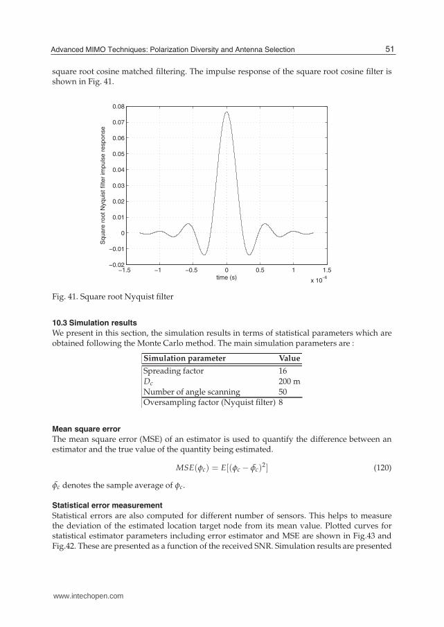
square root cosine matched filtering. The impulse response of the square root cosine filter isshown in Fig. 41.

−1.5 −1 −0.5 0 0.5 1 1.5

x 10−6

−0.02

−0.01

0

0.01

0.02

0.03

0.04

0.05

0.06

0.07

0.08

time (s)

Sq

ua

re r

oo

t N

yq

uis

t filte

r im

pu

lse

re

sp

on

se

Fig. 41. Square root Nyquist filter

10.3 Simulation results

We present in this section, the simulation results in terms of statistical parameters which areobtained following the Monte Carlo method. The main simulation parameters are :

Simulation parameter Value

Spreading factor 16

Dc 200 m

Number of angle scanning 50Oversampling factor (Nyquist filter) 8

Mean square error

The mean square error (MSE) of an estimator is used to quantify the difference between anestimator and the true value of the quantity being estimated.

MSE(φc) = E[(φc − φc)2] (120)

φc denotes the sample average of φc.

Statistical error measurement

Statistical errors are also computed for different number of sensors. This helps to measurethe deviation of the estimated location target node from its mean value. Plotted curves forstatistical estimator parameters including error estimator and MSE are shown in Fig.43 andFig.42. These are presented as a function of the received SNR. Simulation results are presented


www.intechopen.com

for variable numbers of sensors. The obtained results show that the target sensor location isbetter estimated if more collaborative sensors are used. When 16 sensors are introduced, theerror estimation is almost negligible even for low SNR value. We should note that for fartarget sensor node, we obtain higher error estimation. Fig. 44 shows the plotted curves of theestimator error as a function of SNR for D = 200m and D = 400m. 8 collaborative sensors aredeployed in the network.

0 5 10 15 200

0.5

1

1.5

2

2.5

3

3.5

4

4.5

5

SNR(dB)

MS

E (

An

gle

in

De

gre

e)

K=16

K=12

Fig. 42. The mean square error for variable number of sensors

11. Conclusion

Throughout this chapter, we showed that MIMO technology brings significant advances inspectral efficiency by employing several antennas at both ends of the communication system.The geometric channel model was rigorously described and correlated MIMO systems werealso considered. Correlation occurs in rich scattering environment mainly when antennasare spaced close of each others. In this chapter, we were interested by MIMO processingtechniques such as diversity combining, antenna selection and beamforming. Performancesof MIMO systems involving combining techniques were evaluated. We showed thatselection schemes can reduce the system hardware complexity at the mobile while keepingsufficient performance in MIMO systems. Beamforming processing was also presented.Some beamforming scenarios were studied and simulated in this chapter. Then, polarizationdiversity for MIMO systems was investigated and depolarization phenomena was studiedand quantified by the cross polarization discrimination XPD. When orthogonal antennasare used, the spatial correlation effect can be reduced or eliminated due to low radiationpattern interference. Thus, colocated multi polarized antennas can be deployed. Capacitygain for MIMO systems with dual polarized antennas compared to single polarized antennaswas evaluated. Numerical results show that for high XPD values, single polarized antennasperform better. We have finally presented a communication model for WSN involving two


www.intechopen.com

0 5 10 15 200

0.5

1

1.5

2

2.5

3

3.5

4

4.5

SNR(dB)

Sta

tistica

l e

rro

r (A

ng

le in

De

gre

e)

K=16

K=12

K=8

Fig. 43. Statistical error as a function of sensors number K

0 2 4 6 8 102

3

4

5

6

7

8

SNR(dB)

Sta

tistica

l e

rro

r

D=400m

D=200m

Fig. 44. Impact of distance between the source node and the target node


www.intechopen.com

clusters of sensors at both the transmit side and the receive side. The set of sensors locatedat the transmit cluster communicating with sensor nodes located at another cluster performa distributed MIMO system. RSS based localization exploiting beamforming technique wasnumerically developed. The mean square error and the estimator variance associated withthe target sensor location were evaluated as a function of SNR for various parameters ofsimulation. The obtained results show that accurate target sensor localization based onbeamforming processing and RSS measurement could be achieved if the communicationmodel is properly configured. The performed localization technique could be also carried outunder more severe channel environment. Thus, convenient antenna polarization strategy forsensors has to be determined in order to fulfill efficient target sensor localization.

12. References

Ahmed, M.F.A. & Vorobyov, S.A. (2009). Collaborative beamforming for wireless sensornetworks with gaussian distributed sensor nodes, IEEE Transactions on WirelessCommunications Vol. 8(No. 2): 638–643.

Alamouti, S.M. (1998). A simple transmit diversity technique for wireless communications,IEEE Journal on Selected Areas in Communications Vol. 16(No. 8): 1451–1458.

Ben Zid, M., Raoof, K. & Bouallègue, A. (2011). Sensor nodes selection in Wireless SensorNetworks over a rich scattering environment, Accepted for presentation at The IEEE2011 International Conference on Communications, Computing and Control Applications(CCCA’11) and for publication in its proceedings , Tunisia.

Biglieri, E., Calderbank, R., Constantinides, A., Goldsmith, A., Paulraj, A. & Poor, H.(2007). MIMO Wireless Communications, Cambridge University Press, ISBN:978–0–521–87328–4.

Burr, A.G. (2003). Capacity bounds and estimates for the finite scatterers MIMO wirelesschannel, IEEE Journal on Selected Areas in Communications Vol. 21(No. 5): 812–818.

Che-Wei Chang, Kothari, A., Jafri, A., Koutsonikolas, D., Peroulis, D. & Hu, Y.C. (2008).Radiating sensor selection for distributed beamforming in wireless sensor networks,Proceedings of Military Communications Conference (MILCOM), San Diego, pp. 1–7.

Constantine, A.B. (2005). Antenna Theory: Analysis and Design, John Wiley & Sons, Ltd, ISBN:9780471592686, New Jersey.

Dong, Q.T., Prayongpun, N. & Raoof, K. (2008). Antenna selection for MIMO systems incorrelated channels with diversity technique, Proceedings of 4th IEEE InternationalConference on Wireless Communication, Networking and Mobile Computing(WiCOM), Dalian, pp. 1–4.

Foshini, G.F. (1996). Layered space-time architecture for wireless communication in afading environment when using multi-element antennas, Bell Labs Technical Journalpp. 41–59.

Freitas, W.C., Cavalcanti, F.R.P. & Lopes, R.R. (2005). Hybrid transceiver schemes forspatial multiplexing and diversity in MIMO systems, Journal of Communication andInformation Systems Vol. 20(No. 3): 63–76.

Ghrayeb, A. (2006). A survey on antenna selection for MIMO communication systems,Information and Communication Technologie (ICTTA) pp. 2104–2109.

Ibnkahla, M. (2009). Adaptive signal processing in wireless communications, CRC Press, ISBN:978–1–4200–4602–1.

Jafarkhani, H. (2005). Space-Time Coding Theory and Practice, Cambridge University Press,ISBN: 978–0–511–11562–2.


www.intechopen.com

Marzetta, T.L. & Hochwald, B.M. (1999). Capacity of a mobile multiple-antennacommunication link in Rayleigh flat fading, IEEE Transactions on Information TheoryVol. 45(No. 1): 139–157.

Prayongpun, N. (2009). Modélisation et étude de la capacité du canal pour unsystème multi-antennes avancé exploitant la diversité de polarisation, Thesisdissertation-UJF-Grenoble I- Kosai RAOOF (Director) .URL: http://tel.archives-ouvertes.fr/tel-00396666/en/

Proakis, J.G. (1995). Digital Communications, MacGraw-Hill, Inc., ISBN: 0–07–051726–6.Raleigh, G.G. & John, J.M. (1998). Spatio-temporal coding for wireless communication, IEEE

Transactions on Communications Vol. 46(No. 3): 357–366.Raoof, K. & Prayongpun, N. (2005). Channel capacity performance for MIMO polarized

diversity systems, Proceedings of 2005 International Conference on WirelessCommunications, Networking and Mobile Computing , pp. 1–4.

Raoof, K. & Prayongpun, N. (2007). Impact of depolarization effects on MIMOpolarized wireless configuration, Proceedings of International Conference on WirelessCommunications, Networking and Mobile Computing (WiCom), Shanghai, pp. 1–4.

Raoof, K. & Zhou, H. (2009). Advanced MIMO systems, Scientific Research Publishing,ISBN:978–1–935068–02–0.

Saleh, A. & Valenzuela, R. (1987). A statistical model for indoor multipath propagation, IEEEJournal on Selected Areas in Communications Vol. 5(No. 2): 128–137.

Sanayei, S. & Nosratinia, A. (2004). Antenna selection in MIMO systems, IEEE CommunicationsMagazine Vol. 42(No. 10): 68–73.

Shuguang, C., Goldsmith, A.J. & Bahai, A. (2004). Energy-efficiency of MIMO andcooperative MIMO techniques in sensor networks, IEEE Journal On Selected Areas InCommunications Vol. 22(No. 6): 1089–1098.

Tarighat, A., Sadek, M. & Sayed, A.H. (2005). A multi user beamforming scheme for downlinkMIMO channels based on maximizing signal-to-leakage ratios, Proceedings of IEEEInternational Conference on Acoustics, Speech, and Signal Processing., pp. iii/1129–- iii/1132.

Tarokh, V., Jafarkhani, H. & Calderbank, A.R. (1999). Space-time block codes from orthogonaldesigns, IEEE Transactions on Information Theory Vol. 45(No.5): 1456–1467.

Tarokh, V., Seshadri, N. & Calderbank, A.R. (1998). Space-time codes for high datarate wireless communication: Performance criterion and code construction, IEEETransactions on Information Theory Vol. 44(No. 2): 744–765.

Telatar, I. E. (1995). Capacity of multi-antenna gaussian channels, European Transactions onTelecommunications Vol. 10(No. 6): 585–595.

Tran, T.A. & Sesay, A.B. (2003). Orthogonal space-time block codes: performance analysis andcomparisons, Proceedings of Information, Communications and Signal Processing andthe Fourth Pacific Rim Conference on Multimedia, pp. 1497–1501.

Vucetic, B. & Yuan, J. (2003). Space-Time Coding, John Wiley & Sons, Ltd, ISBN: 0–470–84757–3.Wang, C., Hong, X., Ge, X., Cheng, X., Zhang, G. & Thompson, J. (2010). Cooperative MIMO

channel models: A survey, IEEE Communications Magazine Vol. 48(No. 2): 80–87.Winters, J. (1987). On the capacity of radio communication systems with diversity in a

Rayleigh fading environment, IEEE Journal on Selected Areas in Communications Vol.5(No. 5): 871–878.

Yu, W., Cioffi, J. (2001). On constant power water-filling, Proceedings of IEEE InternationalConference on Communications (ICC), Helsinki, pp. 1665–1669.


www.intechopen.com

Yu, C., Ding, Z. & Chiueh, T. (2004). Design and simulation of a MIMO OFDM basebandtransceiver for high throughput wireless LAN, Proceedings of The 2004 IEEEAsia-Pacific Conference on Circuits and Systems, Taiwan, pp. 205 – 208.

Zheng, L. & Tse, D.N.C. (2003). Diversity and multiplexing: a fundamental tradeoffin multiple-antenna channels, IEEE Transactions on Information Theory Vol. 49(No.5): 1073–1096.

Zhou, H. & Okamoto, K. (2004). Comparison of code combining and MRC diversity receptionin mobile communications, Proceedings of 2004 IEEE Wireless Communications andNetworking Conference (WCNC), pp. 943–947.


www.intechopen.com

MIMO Systems, Theory and ApplicationsEdited by Dr. Hossein Khaleghi Bizaki

ISBN 978-953-307-245-6Hard cover, 488 pagesPublisher InTechPublished online 04, April, 2011Published in print edition April, 2011

InTech EuropeUniversity Campus STeP Ri Slavka Krautzeka 83/A 51000 Rijeka, Croatia Phone: +385 (51) 770 447 Fax: +385 (51) 686 166www.intechopen.com

InTech ChinaUnit 405, Office Block, Hotel Equatorial Shanghai No.65, Yan An Road (West), Shanghai, 200040, China

Phone: +86-21-62489820 Fax: +86-21-62489821

In recent years, it was realized that the MIMO communication systems seems to be inevitable in acceleratedevolution of high data rates applications due to their potential to dramatically increase the spectral efficiencyand simultaneously sending individual information to the corresponding users in wireless systems. This book,intends to provide highlights of the current research topics in the field of MIMO system, to offer a snapshot ofthe recent advances and major issues faced today by the researchers in the MIMO related areas. The book iswritten by specialists working in universities and research centers all over the world to cover the fundamentalprinciples and main advanced topics on high data rates wireless communications systems over MIMOchannels. Moreover, the book has the advantage of providing a collection of applications that are completelyindependent and self-contained; thus, the interested reader can choose any chapter and skip to anotherwithout losing continuity.

How to referenceIn order to correctly reference this scholarly work, feel free to copy and paste the following:

Kosai Raoof, Maha Ben Zid, Nuttapol Prayongpun and Ammar Bouallegue (2011). Advanced MIMOTechniques: Polarization Diversity and Antenna Selection, MIMO Systems, Theory and Applications, Dr.Hossein Khaleghi Bizaki (Ed.), ISBN: 978-953-307-245-6, InTech, Available from:http://www.intechopen.com/books/mimo-systems-theory-and-applications/advanced-mimo-techniques-polarization-diversity-and-antenna-selection

© 2011 The Author(s). Licensee IntechOpen. This chapter is distributedunder the terms of the Creative Commons Attribution-NonCommercial-ShareAlike-3.0 License, which permits use, distribution and reproduction fornon-commercial purposes, provided the original is properly cited andderivative works building on this content are distributed under the samelicense.

https://creativecommons.org/licenses/by-nc-sa/3.0/

Advanced MIMO Techniques: Polarization Diversity and...

Documents

Transcript of Advanced MIMO Techniques: Polarization Diversity and...