Introduction Example Existence Welfare Discussion Conclusions

Advanced MicroeconomicsPartial and General Equilibrium

Giorgio Fagiologiorgio.fagiolo@sssup.it

http://www.lem.sssup.it/fagiolo/Welcome.html

LEM, Sant’Anna School of Advanced Studies, Pisa (Italy)

Part 4

Spring 2011

Introduction Example Existence Welfare Discussion Conclusions

Recap

So far: We have been studying reductions of the full-fledged GE model tosimplify the analysis

1 Reducing the number of markets to only one, while keeping manyconsumers and firms: partial-equilibrium analysis

2 Reducing the number of firms to zero, while keeping many markets andconsumers: pure-exchange analysis

Now: Analyzing the full-fledged GE model, but starting with yet anothersimplification

3 Allowing for 2 markets, 1 consumer and 1 firm (Robinson Crusoe’seconomy)

Introduction Example Existence Welfare Discussion Conclusions

The Full-Fledged Model

Consider a model of a decentralized economy E with the followingingredients:

Consumers: i = 1, ..., IFirms: j = 1, ..., J

Commodities: l = 1, ..., L

Let us also assume that:

Each consumer i has preferences (i ,Xi ) and an associated (continuous) utilityfunction ui which maps consumption bundles xi = (x1i , ..., xLi ) ∈ Xi into <; andholds an initial endowment vector ωi ∈ <L

+; ; let Ω = (ω1, ..., ωI) andω =

∑i ωi ∈ <L

+

Each firm j holds a technology Yj ⊆ <L and define ylj as the netput of firm j forcommodity l ; hence, the “net amount” available for good l will be: ωl +

∑j ylj

Introduction Example Existence Welfare Discussion Conclusions

The Full-Fledged Model

Moreover, assume that:

Private Ownership: Consumers own firms. Each consumer holds a share θij ≥ 0of firm j , s.t.

∑i θij = 1, all j , i.e. θi ∈ [0, 1]J . Profits are entirely redistributed to

consumers accordingly to shares.Markets are complete (there exist L markets for the L commodities).Commodities are undifferentiated (homogeneous). No firms have then advantagewhatsoever in selling them and consumers cannot discriminate betweencommodities sold by different firms.There is perfect information about prices across agents. Consumers and firmsare perfectly rational (maximizers) and act as price takers.

All actual exchanges take place simultaneously at a single price vector, after thelatter has been quoted. If a firm sells at lower prices, she will undercutcompetitors. Reselling is not allowed. Pricing is linear (every unit of commoditiesis sold at the same unit price).

As a result, the economy will be completely defined by:

E =(Xi , uiI

i=1, YjJj=1; ωi , θiI

i=1

)

Introduction Example Existence Welfare Discussion Conclusions

Competitive (Walrasian) Equilibrium

Definition (Competitive (Walrasian) Equilibrium)

An allocation (x∗i )Ii=1, (y∗j )J

j=1 and a price vector p∗ ∈ <L++ is a Competitive (or

Walrasian) Equilibrium (CE) for the economy E iff the following three conditions aresatisfied:

1 (Profit Maximization): Given p∗, then y∗j = arg max(p∗yj ), s.t. yj ∈ Yj ,∀j = 1, ..., J

2 (Utility Maximization): Given Condition 1 and p∗, then x∗i = arg max ui (xi ), s.t.p∗xi ≤ p∗ωi +

∑j θij p∗y∗j , xi ∈ Xi , ∀i = 1, ..., I

3 (Market Clearing):∑

i x∗li ≤∑

i ωli +∑

j y∗lj , ∀l = 1, ..., L

Introduction Example Existence Welfare Discussion Conclusions

A Robinson Crusoe’s Economy

Consider a general-equilibrium model of an economy composed of a singleproducer and a single consumer. Ingredients:

1 price-taker consumers (I = 1)

1 price-taker firm (J = 1)

Two goods (L = 2): Labor/leisure (input) and consumption good (output)

Labor is used to produce output consumption good

Endowments: ωL = L (hours), ωc = 0 (must be produced)

Preferences: u(x1, x2) = u(L, x), where L=leisure (L-labor),x=consumption good

Technology: f : R+ → R+, where y = f (z)=consumption good efficientlyproduced with z units of labor

Prices (p,w), p=consumption good price, w=labor price (unit wage)

Therefore: RC owns the firm, works for the firm, gets wage and buys theconsumption good that the firm produces (. . . a rather weird institutionalsetting!)

Introduction Example Existence Welfare Discussion Conclusions

A Robinson Crusoe’s Economy

RC as a firmSolves maxz pf (z)− wzLabor demand: z(p,w)Output function: q(p,w)Profit function: π(p,w)

RC as a consumerSolves maxL,x u(L, x), s.t. px + wL ≤ wL + π(p,w)Leisure: L(p,w)Labor: L− L(p,w)Consumption good: x(p,w)

AssumptionsStrictly convex, strictly monotone preferencesStrictly convex technologies

General equilibrium: It is a p∗/w∗ ratio such that1 x(p∗,w∗) = q(p∗,w∗)2 L− L(p∗,w∗) = z(p∗,w∗)

Introduction Example Existence Welfare Discussion Conclusions

A Robinson Crusoe’s Economy

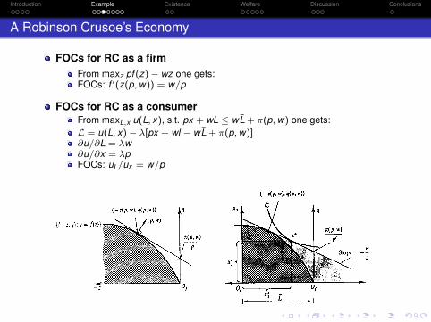
FOCs for RC as a firmFrom maxz pf (z)− wz one gets:FOCs: f ′(z(p,w)) = w/p

FOCs for RC as a consumerFrom maxL,x u(L, x), s.t. px + wL ≤ wL + π(p,w) one gets:L = u(L, x)− λ[px + wl − wL + π(p,w)]∂u/∂L = λw∂u/∂x = λpFOCs: uL/ux = w/p

Introduction Example Existence Welfare Discussion Conclusions

A Robinson Crusoe’s Economy: Equilibrium

f ′(z(p∗,w∗)) =w∗

p∗=

uL

ux

x(p∗,w∗) = q(p∗,w∗)

If (p∗,w∗) is a WE, then RC maximizes utilitywhile satisfying technological and resourceconstraints. Therefore the resulting allocation isPO (1st welfare theorem revisited). It is easy tosee that also the 2nd WT holds (given convexityassumptions).

Introduction Example Existence Welfare Discussion Conclusions

A Robinson Crusoe’s Economy: Non-Convex Technology

The case of non-convex technologies. In x∗ the consumer is maximizing his utility andits welfare and the allocation is PO. However, at the unique price ratio that supports thisallocation the firm is not maximizing her profits since her technology exhibits increasingreturns to scale (she would prefer to use more labor). Therefore the 2nd WT failsbecause there is no price vector supporting the PO allocation x∗.

Introduction Example Existence Welfare Discussion Conclusions

A Robinson Crusoe’s Economy: Non-Convex Technology

Even if technology presents some non-convexities the 1st WT applies. The allocationand price vector (x∗, p∗,w∗) is a WE and the consumer is maximizing her welfare.

Introduction Example Existence Welfare Discussion Conclusions

What’s Next

So far: Showing that in a RC economy with some peculiar features(convexity throughout) an equilibrium exists and welfare theorems apply

Now: Analyzing the full-fledged GE model with many markets, manyconsumers, and many firms. We ask two questions:

1 Does an equilibrium always exist? If not, what are sufficient conditionsguaranteeing existence of (at least one) equilibrium?

2 If an equilibrium exists, do the 1st and 2nd welfare theorem apply in themost general setting? Under what conditions?

Introduction Example Existence Welfare Discussion Conclusions

Excess of Demand

The ’production-inclusive excess of demand’ (excess demand in what follows) is thefunction/ correspondence that we obtain by computing the difference betweenMarshallian demand functions/correspondences (given profitfunctions/correspondences) and net amount of available commodities (initialendowments plus net supply)

More formally: For any price vector p 0, define the ’excess of demand’z : <L

++ → <L as

z(p) =I∑

i=1

xi (p, pωi +∑

j

θijπj (p))−

I∑i=1

ωi +J∑

j=1

yj (p)

where xi (·, ·) is the Marshallian demand function of consumer i ; πj (p) and yj (p) are theprofit- and the net-supply functions/correspondences of firm j .

Obviously (but try to prove it formally!) we have that: p∗ 0 is a price-equilibriumvector if and only if z(p∗) = 0.

Studying the existence of a CE means studying whether a p∗ 0 exists which solvesthe system in L equations and L unknowns defined by z(p) = 0.

Introduction Example Existence Welfare Discussion Conclusions

Existence of a Walrasian Equilibrium

Claim

Assume that:

1 Utility functions ui are continuous, strictly increasing and concave;2 Technology sets Yj are closed, convex and bounded from above;

3 By using ω =∑I

i=1 ωi it is possible to produce a strictly positive consumptionbundle x 0.

Then there exists a p∗ 0 such that z(p∗) = 0.

Proof.

See Mas-Colell, Whinston and Green, Ch. 17.A, 17.B, 17.C. For a historicalperspective, see Ingrao and Israel (1990).

Introduction Example Existence Welfare Discussion Conclusions

First Welfare Theorem

Theorem (First Welfare Theorem in a General Equilibrium Model with Production)

Suppose that (x∗i )Ii=1, (y∗j )J

j=1 and p∗ is a competitive equilibrium for the associatedeconomy E and that utility functions ui all satisfy local non-satiation. Then theallocation (x∗i )I

i=1, (y∗j )Jj=1 is Pareto Efficient.

Proof.

Suppose (x∗i )Ii=1, (y∗j )J

j=1 and p∗ is a competitive equilibrium for E . Define:

wi = p∗ωi +∑

j

θij p∗y∗j

Notice that: ∑i

wi = p∗∑

i

ωi +∑

j

p∗y∗j

Equilibrium conditions read: (1) ∀j : p∗yj ≤ p∗y∗j , ∀yj ∈ Yj ;(2) ∀i : ui (xi ) ≤ ui (x∗i ),

∀xi ∈ Xi such that p∗xi ≤ wi ; (3)∑

i x∗i =∑

i ωi +∑

j y∗j .

Introduction Example Existence Welfare Discussion Conclusions

First Welfare Theorem

Proof (Cont’d).

By (2) above, we know that:

ui (xi ) > ui (x∗i ) implies that p∗xi > wi .

Moreover, by local non-satiation (LNS) we also know that:

ui (xi ) ≥ ui (x∗i ) implies that p∗xi ≥ wi .

To see this, suppose that ui (xi ) ≥ ui (x∗i ) implied that p∗xi < wi . Then by LNS ∃ x ′isufficiently close to xi which is strictly preferred to xi but is still strictly affordable, i.e.p∗x ′i < wi . Then ui (x ′i ) > ui (x∗i ) and p∗x ′i < wi which contradicts the hypothesis thatx∗i is a utility maximizing bundle.

Introduction Example Existence Welfare Discussion Conclusions

First Welfare Theorem

Proof (Cont’d).

We are then ready to show that the allocation (x∗i )Ii=1, (y∗j )J

j=1 is Pareto Efficient.Suppose not. In this case, there will exist another feasible allocation (xi )

Ii=1, (yj )

Jj=1

such that:

ui (xi ) ≥ ui (x∗i ) ∀iuh(xh) > uh(x∗h ) some h

As a consequence:

p∗xi ≥ wi ∀ip∗xh > wh some h

Summing up over all i ′s:∑i

p∗xi >∑

i

wi = p∗∑

i

ωi +∑

j

p∗y∗j

Introduction Example Existence Welfare Discussion Conclusions

First Welfare Theorem

Proof (Cont’d).

Since y∗j maximizes j ′s profits, then ∀j : p∗y∗j ≥ p∗yj . Hence:∑i

p∗xi > p∗∑

i

ωi +∑

j

p∗y∗j ≥ p∗∑

i

ωi +∑

j

p∗yj

so that:

p∗

∑i

xi −∑

i

ωi −∑

j

yj

> 0

And as p∗ 0, then∑

i xi −∑

i ωi −∑

j yj 6= 0, which means the the allegedallocation is not feasible. This contradicts the thesis that (x∗i )I

i=1, (y∗j )Jj=1 is not Pareto

Efficient.

Introduction Example Existence Welfare Discussion Conclusions

Second Welfare Theorem

Theorem (Second Welfare Theorem in a General Equilibrium Model with Production)

Suppose E is such that: (1) Production sets are convex; (2) Utility functions ui haveconvex upper contour sets and satisfy LNS. Then if the allocation (x∗i )I

i=1, (y∗j )Jj=1 is

Pareto Efficient, there exists a redistribution of endowments and profits such that(x∗i )I

i=1, (y∗j )Jj=1 and p∗ is a WE.

Proof.

See Mas-Colell, Whinston and Green, Ch. 16.D.

Introduction Example Existence Welfare Discussion Conclusions

The GE Model

We have shown that, under some restrictions, there are very stringentrelationships between concepts as decentralized CE, PO allocations andsocial welfare optima.

Suppose that we are given an economy

E =(Xi , uiI

i=1, YjJj=1; ωi , θiI

i=1

)where all assumptions made at the beginning apply.

Introduction Example Existence Welfare Discussion Conclusions

The GE Model

1 If a CE (p∗, (x∗i )Ii=1, (y∗j )J

j=1) exists for E , then irrespective of anyconvexity assumption, the allocation (x∗i )I

i=1, (y∗j )Jj=1 is a Pareto

Optimum. Moreover, if U is convex and the SWF is linear, then thereexist weights λ∗ ≥ 0 such that the associated utility levels maximize theSWF (i.e. the correspondent allocation would have been chosen by abenevolent planner).

2 Irrespective of any convexity assumption, if the allocation (x∗i )Ii=1, (y∗j )J

j=1corresponds to a social welfare optimum chosen by the benevolentplanner for some λ∗ ≥ 0, then (x∗i )I

i=1, (y∗j )Jj=1 is PO. Moreover, under

some convexity assumptions (see Second Welfare Theorem), thereexists a price vector p∗ 0 and a redistribution of endowments andprofits such that (x∗i )I

i=1, (y∗j )Jj=1 can be sustained by p∗ as a CE.

Introduction Example Existence Welfare Discussion Conclusions

The GE Model

Therefore:

If a planner maximizes W , s/he reaches a PO allocation, but only underconvexity assumptions this allocation is supported by equilibrium prices.

If we let the economy work, then we reach a PO allocation, but onlyunder convexity assumptions this allocation is socially fair.

The allocation maximizessocial welfare for some

choice of weights

(x∗)i, (y∗)j

λ∗

The allocation is a Pareto optimum

(x∗)i, (y∗)j

Conv

exity

p∗, (x∗)i, (y∗)j

The price-allocation

is a competitive equilibrium

Conv

exity

Introduction Example Existence Welfare Discussion Conclusions

What’s Next

So far: We have established that if the economy satisfies certain (verystringent) properties, then at least one WE exists. We are left with othercrucial questions to answer. . .

1 Uniqueness: When a WE exists, is it unique? How many WE are there?

2 Stability: Suppose that a unique WE does exist. How does the economy(as distinct from the modeler) “find” the equilibrium, i.e. how does it gothere? And if the economy starts far from the equilibrium, is it able toactually go back to the WE?

3 Empirical validity: Can we take the GET to the data and test whether itsimplications are true? What implications can we test?