Advanced Microeconomic Theory · Theory Chapter 3: Demand Theory Applications. ... Price Change •...
108
Advanced Microeconomic Theory Chapter 3: Demand Theory Applications
Transcript of Advanced Microeconomic Theory · Theory Chapter 3: Demand Theory Applications. ... Price Change •...

Advanced Microeconomic Theory
Chapter 3: Demand Theory Applications

Outline
• Welfare evaluation– Compensating variation– Equivalent variation
• Quasilinear preferences• Slutsky equation revisited• Income and substitution effects in labor
markets• Gross and net substitutability• Aggregate demand
Advanced Microeconomic Theory 2

Measuring the Welfare Effects of a Price Change
Advanced Microeconomic Theory 3

Measuring the Welfare Effects of a Price Change
• How can we measure the welfare effects of:– a price decrease/increase– the introduction of a tax/subsidy
• Why not use the difference in the individual’s utility level, i.e., from 𝑢𝑢0 to 𝑢𝑢1?– Two problems:
1) Within a subject criticism: Only ranking matters (ordinality), not the difference;
2) Between a subject criticism: Utility measures would not be comparable among different individuals.
• Instead, we will pursue monetary evaluations of such price/tax changes.
Advanced Microeconomic Theory 4
Measuring the Welfare Effects of a Price Change
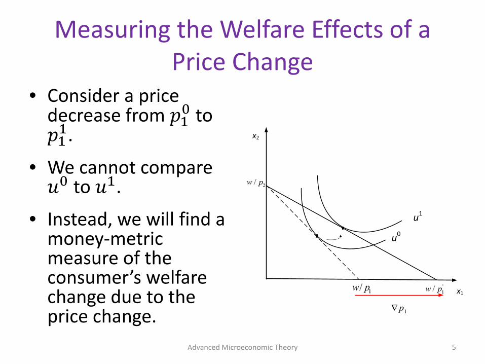
• Consider a price decrease from 𝑝𝑝1
0 to 𝑝𝑝1
1.
• We cannot compare 𝑢𝑢0 to 𝑢𝑢1.
• Instead, we will find a money-metric measure of the consumer’s welfare change due to the price change.
Advanced Microeconomic Theory 5
x2
x1
u1
u0

Measuring the Welfare Effects of a Price Change
• Compensating Variation (CV):– How much money a consumer would be willing to
give up after a reduction in prices to be just as well off as before the price decrease.
• Equivalent Variation (EV): – How much money a consumer would need before
a reduction in prices to be just as well off as afterthe price decrease.
Advanced Microeconomic Theory 6

Measuring the Welfare Effects of a Price Change
• Two approaches:1) Using expenditure function2) Using the Hicksian demand
Advanced Microeconomic Theory 7

CV using Expenditure Function
• 𝐶𝐶𝐶𝐶(𝑝𝑝0, 𝑝𝑝1, 𝑤𝑤) using 𝑒𝑒(𝑝𝑝, 𝑢𝑢):
𝐶𝐶𝐶𝐶 𝑝𝑝0, 𝑝𝑝1, 𝑤𝑤 = 𝑒𝑒 𝑝𝑝1, 𝑢𝑢1 − 𝑒𝑒 𝑝𝑝1, 𝑢𝑢0
• The amount of money the consumer is willing to give up after the price decrease (after price level is 𝑝𝑝1 and her utility level has improved to 𝑢𝑢1) to be just as well off as before the price decrease (reaching utility level 𝑢𝑢0).
Advanced Microeconomic Theory 8
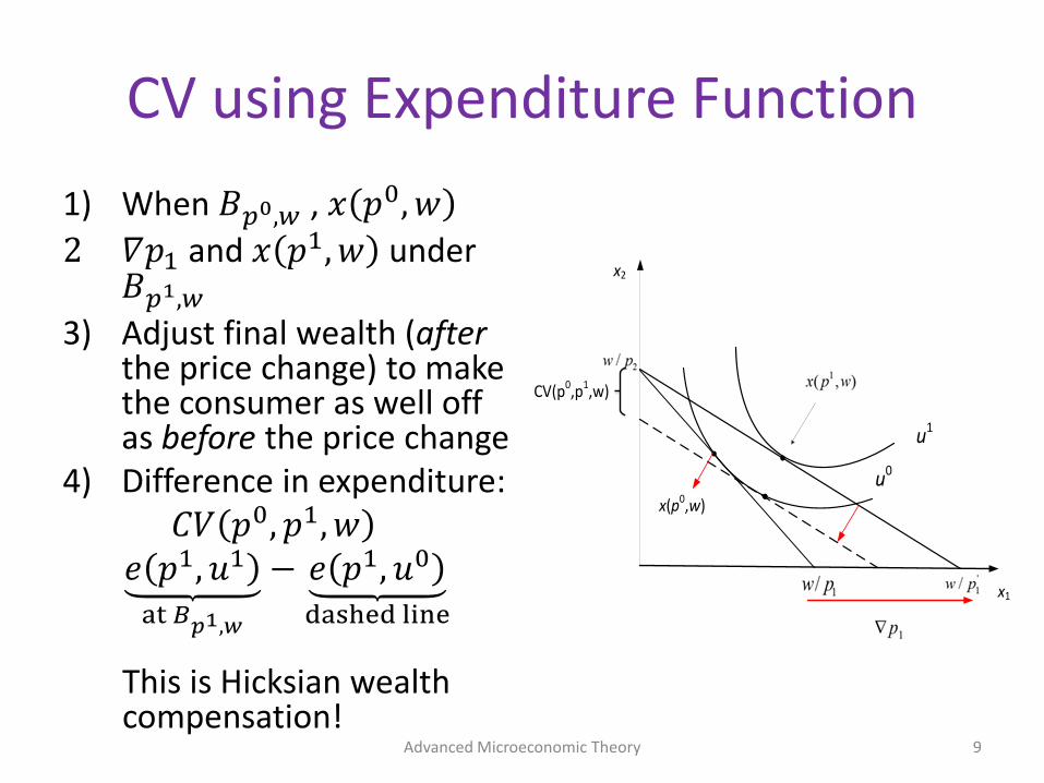
CV using Expenditure Function1) When 𝐵𝐵𝑝𝑝0,𝑤𝑤 , 𝑥𝑥 𝑝𝑝0, 𝑤𝑤2) 𝛻𝛻𝑝𝑝1 and 𝑥𝑥 𝑝𝑝1, 𝑤𝑤 under
𝐵𝐵𝑝𝑝1,𝑤𝑤3) Adjust final wealth (after
the price change) to make the consumer as well off as before the price change
4) Difference in expenditure:𝐶𝐶𝐶𝐶 𝑝𝑝0, 𝑝𝑝1, 𝑤𝑤 =
𝑒𝑒 𝑝𝑝1, 𝑢𝑢1
at 𝐵𝐵𝑝𝑝1,𝑤𝑤
− 𝑒𝑒 𝑝𝑝1, 𝑢𝑢0
dashed line
This is Hicksian wealth compensation!
Advanced Microeconomic Theory 9
x2
x1
u1
u0
CV(p0,p1,w)
x(p0,w)
EV using Expenditure Function
• 𝐸𝐸𝐶𝐶(𝑝𝑝0, 𝑝𝑝1, 𝑤𝑤) using 𝑒𝑒(𝑝𝑝, 𝑢𝑢):
𝐸𝐸𝐶𝐶 𝑝𝑝0, 𝑝𝑝1, 𝑤𝑤 = 𝑒𝑒 𝑝𝑝0, 𝑢𝑢1 − 𝑒𝑒 𝑝𝑝0, 𝑢𝑢0
• The amount of money the consumer needs to receive before the price decrease (at the initial price level 𝑝𝑝0 when her utility level is still 𝑢𝑢0) to be just as well off as after the price decrease (reaching utility level 𝑢𝑢1).
Advanced Microeconomic Theory 10
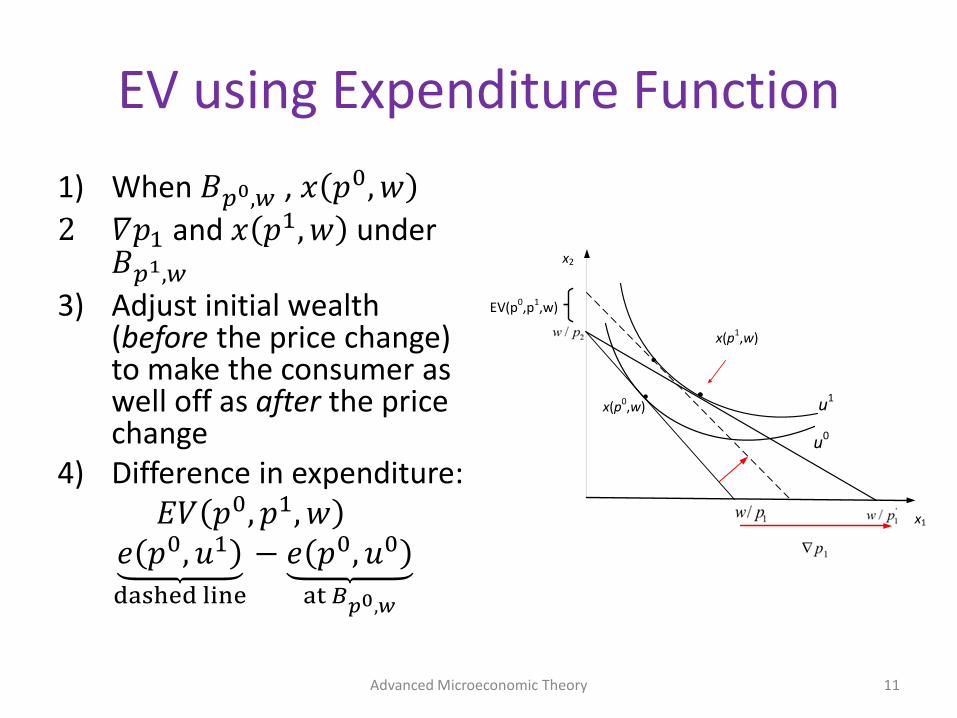
EV using Expenditure Function1) When 𝐵𝐵𝑝𝑝0,𝑤𝑤 , 𝑥𝑥 𝑝𝑝0, 𝑤𝑤2) 𝛻𝛻𝑝𝑝1 and 𝑥𝑥 𝑝𝑝1, 𝑤𝑤 under
𝐵𝐵𝑝𝑝1,𝑤𝑤3) Adjust initial wealth
(before the price change) to make the consumer as well off as after the price change
4) Difference in expenditure:𝐸𝐸𝐶𝐶 𝑝𝑝0, 𝑝𝑝1, 𝑤𝑤 =
𝑒𝑒 𝑝𝑝0, 𝑢𝑢1
dashed line− 𝑒𝑒 𝑝𝑝0, 𝑢𝑢0
at 𝐵𝐵𝑝𝑝0,𝑤𝑤
Advanced Microeconomic Theory 11
x2
x1
u1
u0
EV(p0,p1,w)
x(p1,w)
x(p0,w)
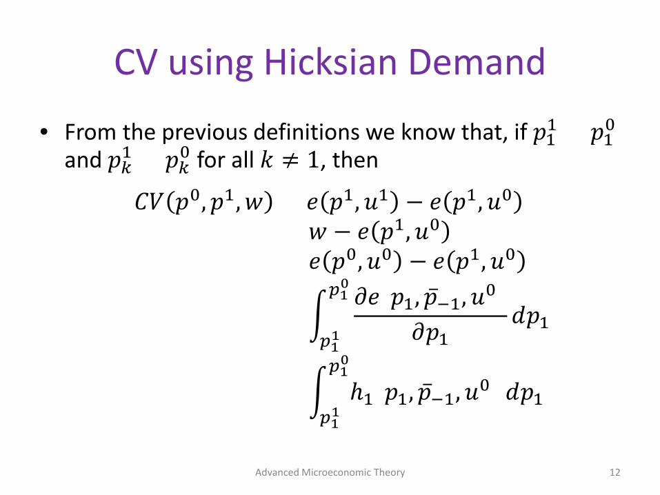
CV using Hicksian Demand
• From the previous definitions we know that, if 𝑝𝑝11 < 𝑝𝑝1
0
and 𝑝𝑝𝑘𝑘1 = 𝑝𝑝𝑘𝑘
0 for all 𝑘𝑘 ≠ 1, then
𝐶𝐶𝐶𝐶 𝑝𝑝0, 𝑝𝑝1, 𝑤𝑤 = 𝑒𝑒 𝑝𝑝1, 𝑢𝑢1 − 𝑒𝑒 𝑝𝑝1, 𝑢𝑢0
= 𝑤𝑤 − 𝑒𝑒 𝑝𝑝1, 𝑢𝑢0
= 𝑒𝑒 𝑝𝑝0, 𝑢𝑢0 − 𝑒𝑒 𝑝𝑝1, 𝑢𝑢0
= �𝑝𝑝1
1
𝑝𝑝10
𝜕𝜕𝑒𝑒(𝑝𝑝1, ��𝑝−1, 𝑢𝑢0)𝜕𝜕𝑝𝑝1
𝑑𝑑𝑝𝑝1
= �𝑝𝑝1
1
𝑝𝑝10
ℎ1(𝑝𝑝1, ��𝑝−1, 𝑢𝑢0) 𝑑𝑑𝑝𝑝1
Advanced Microeconomic Theory 12
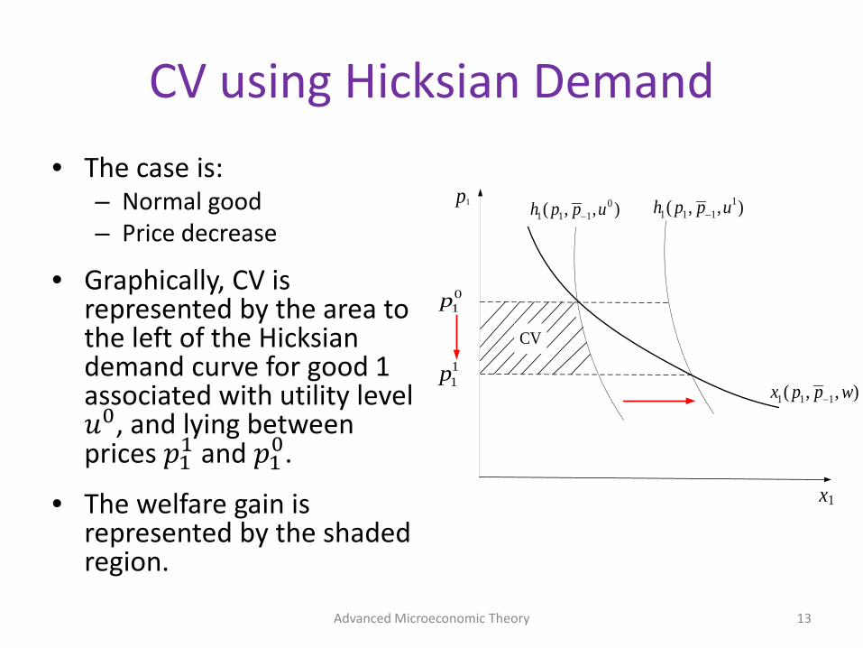
CV using Hicksian Demand• The case is:
– Normal good– Price decrease
• Graphically, CV is represented by the area to the left of the Hicksian demand curve for good 1 associated with utility level 𝑢𝑢0, and lying between prices 𝑝𝑝1
1 and 𝑝𝑝10.
• The welfare gain is represented by the shaded region.
Advanced Microeconomic Theory 13
p1
x1
01p
11p
CV
01 1 1( , , )h p p u−
11 1 1( , , )h p p u−
1 1 1( , , )x p p w−
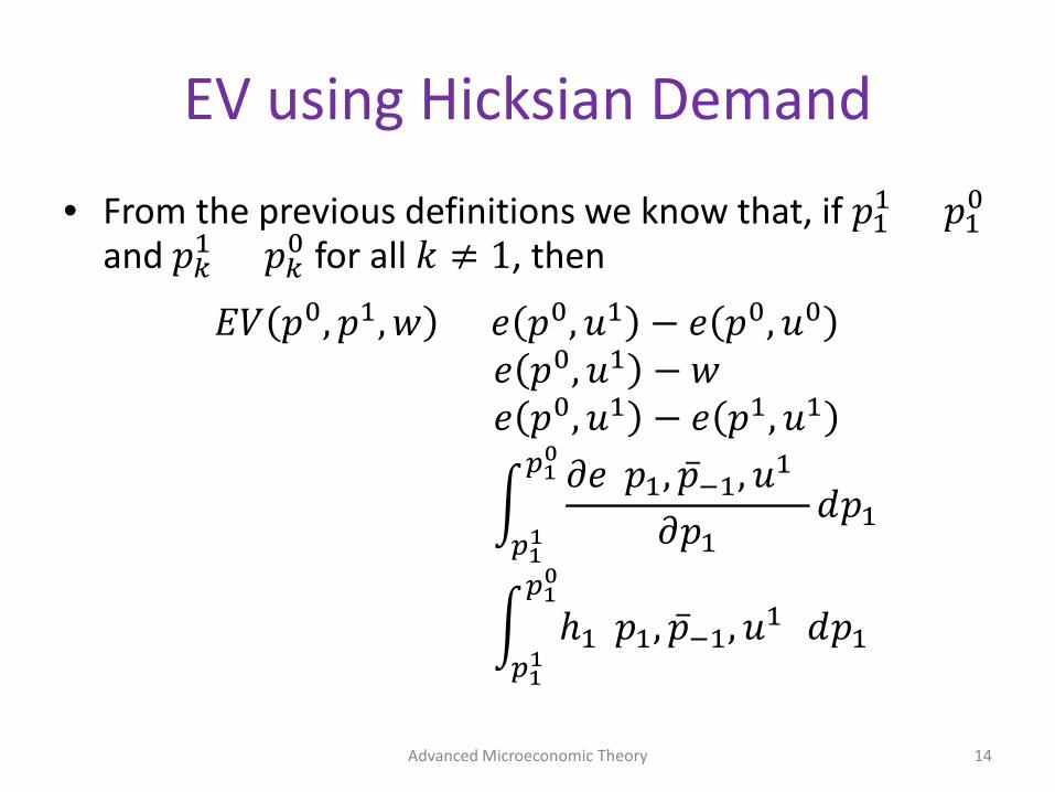
EV using Hicksian Demand
• From the previous definitions we know that, if 𝑝𝑝11 < 𝑝𝑝1
0
and 𝑝𝑝𝑘𝑘1 = 𝑝𝑝𝑘𝑘
0 for all 𝑘𝑘 ≠ 1, then
𝐸𝐸𝐶𝐶 𝑝𝑝0, 𝑝𝑝1, 𝑤𝑤 = 𝑒𝑒 𝑝𝑝0, 𝑢𝑢1 − 𝑒𝑒 𝑝𝑝0, 𝑢𝑢0
= 𝑒𝑒 𝑝𝑝0, 𝑢𝑢1 − 𝑤𝑤= 𝑒𝑒 𝑝𝑝0, 𝑢𝑢1 − 𝑒𝑒 𝑝𝑝1, 𝑢𝑢1
= �𝑝𝑝1
1
𝑝𝑝10
𝜕𝜕𝑒𝑒(𝑝𝑝1, ��𝑝−1, 𝑢𝑢1)𝜕𝜕𝑝𝑝1
𝑑𝑑𝑝𝑝1
= �𝑝𝑝1
1
𝑝𝑝10
ℎ1(𝑝𝑝1, ��𝑝−1, 𝑢𝑢1) 𝑑𝑑𝑝𝑝1
Advanced Microeconomic Theory 14
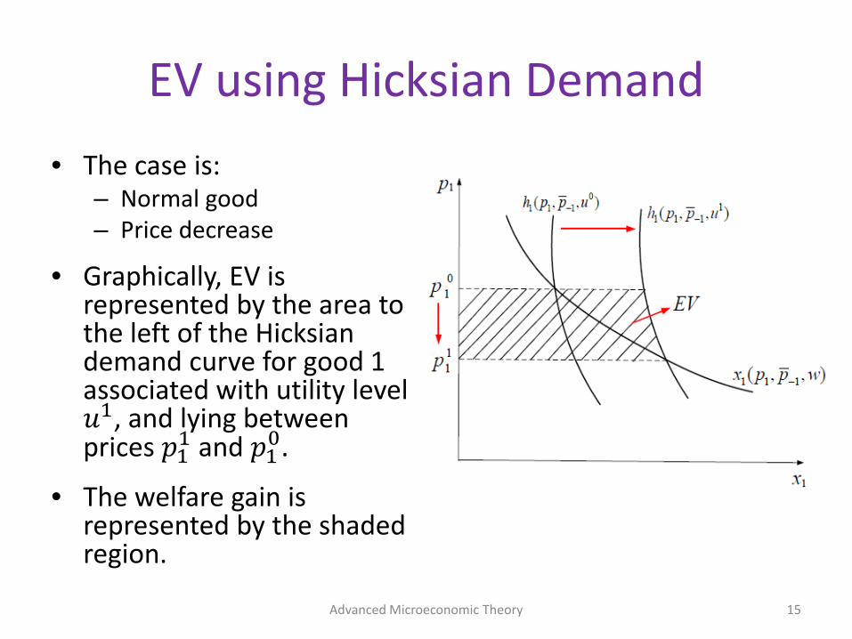
EV using Hicksian Demand• The case is:
– Normal good– Price decrease
• Graphically, EV is represented by the area to the left of the Hicksian demand curve for good 1 associated with utility level 𝑢𝑢1, and lying between prices 𝑝𝑝1
1 and 𝑝𝑝10.
• The welfare gain is represented by the shaded region.
Advanced Microeconomic Theory 15

What about a price increase?
• The Hicksian demand associated with initial utility level 𝑢𝑢0 (before the price increase, or before the introduction of a tax) experiences an inward shift when the price increases, or when the tax is introduced, since the consumer’s utility level is now 𝑢𝑢1, where 𝑢𝑢0 >𝑢𝑢1. Hence,
ℎ1 𝑝𝑝1, ��𝑝−1, 𝑢𝑢0 > ℎ1(𝑝𝑝1, ��𝑝−1, 𝑢𝑢1)
Advanced Microeconomic Theory 16
What about a price increase?
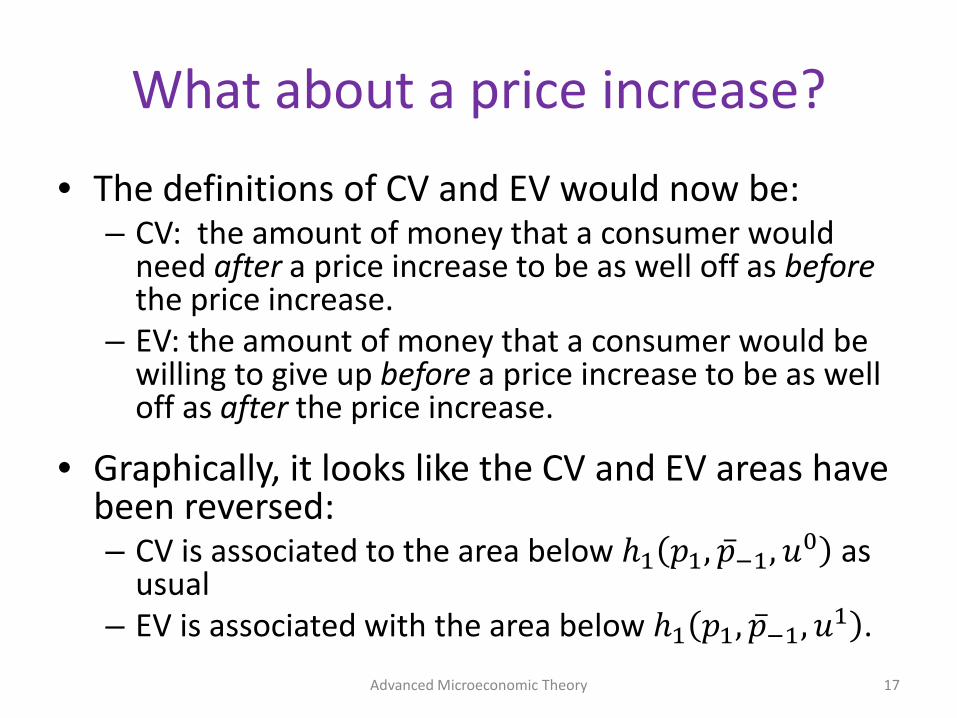
• The definitions of CV and EV would now be:– CV: the amount of money that a consumer would
need after a price increase to be as well off as beforethe price increase.
– EV: the amount of money that a consumer would be willing to give up before a price increase to be as well off as after the price increase.
• Graphically, it looks like the CV and EV areas have been reversed:– CV is associated to the area below ℎ1 𝑝𝑝1, ��𝑝−1, 𝑢𝑢0 as
usual– EV is associated with the area below ℎ1 𝑝𝑝1, ��𝑝−1, 𝑢𝑢1 .
Advanced Microeconomic Theory 17
What about a price increase?
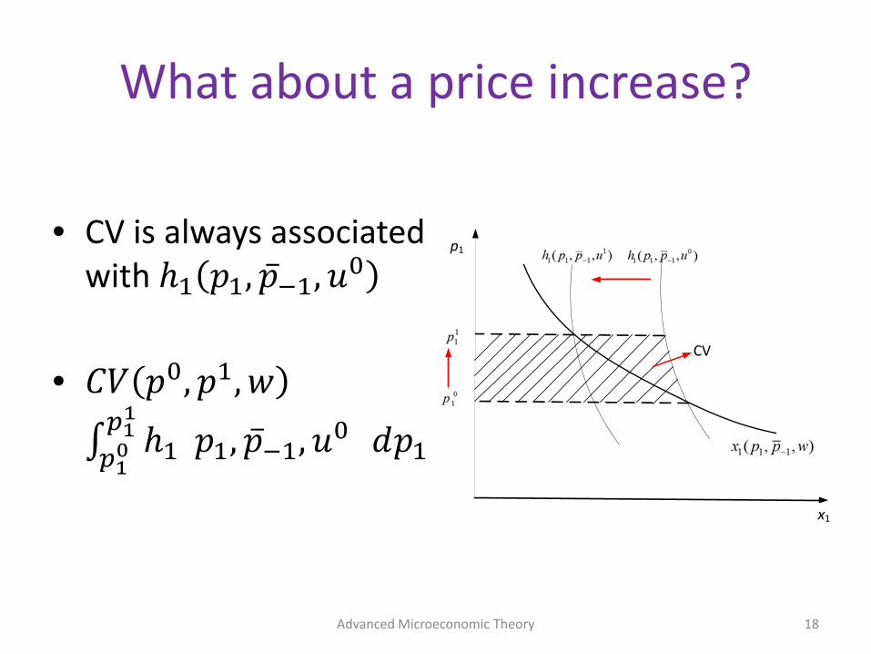
• CV is always associated with ℎ1 𝑝𝑝1, ��𝑝−1, 𝑢𝑢0
• 𝐶𝐶𝐶𝐶 𝑝𝑝0, 𝑝𝑝1, 𝑤𝑤 =
∫𝑝𝑝10
𝑝𝑝11
ℎ1(𝑝𝑝1, ��𝑝−1, 𝑢𝑢0) 𝑑𝑑𝑝𝑝1
Advanced Microeconomic Theory 18
x1
CV
p1

What about a price increase?
• EV is always associated with ℎ1 𝑝𝑝1, ��𝑝−1, 𝑢𝑢1
• 𝐸𝐸𝐶𝐶 𝑝𝑝0, 𝑝𝑝1, 𝑤𝑤 =
∫𝑝𝑝10
𝑝𝑝11
ℎ1(𝑝𝑝1, ��𝑝−1, 𝑢𝑢1) 𝑑𝑑𝑝𝑝1
Advanced Microeconomic Theory 19
X1
EV
p1
Introduction of a Tax
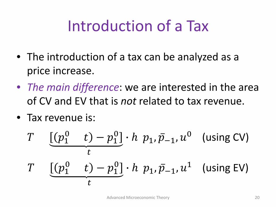
• The introduction of a tax can be analyzed as a price increase.
• The main difference: we are interested in the area of CV and EV that is not related to tax revenue.
• Tax revenue is:
𝑇𝑇 = 𝑝𝑝10 + 𝑡𝑡 − 𝑝𝑝1
0 �𝑡𝑡
ℎ(𝑝𝑝1, ��𝑝−1, 𝑢𝑢0) (using CV)
𝑇𝑇 = 𝑝𝑝10 + 𝑡𝑡 − 𝑝𝑝1
0 �𝑡𝑡
ℎ(𝑝𝑝1, ��𝑝−1, 𝑢𝑢1) (using EV)
Advanced Microeconomic Theory 20
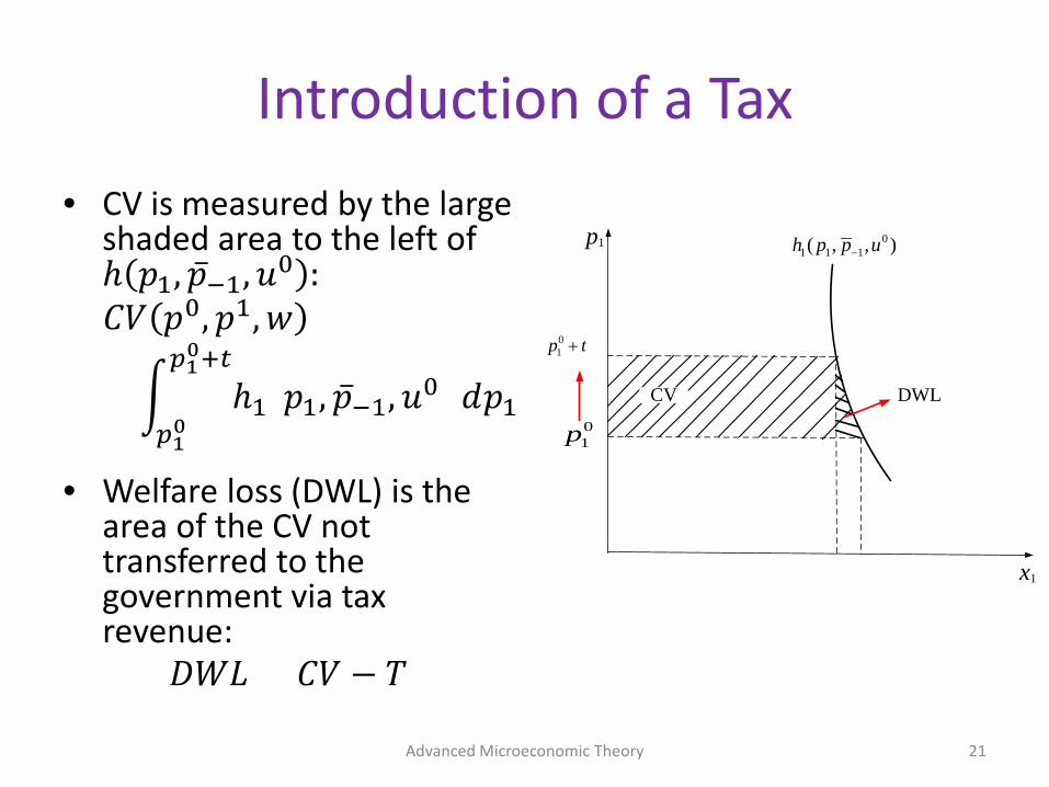
Introduction of a Tax• CV is measured by the large
shaded area to the left of ℎ 𝑝𝑝1, ��𝑝−1, 𝑢𝑢0 :𝐶𝐶𝐶𝐶 𝑝𝑝0, 𝑝𝑝1, 𝑤𝑤
= �𝑝𝑝1
0
𝑝𝑝10+𝑡𝑡
ℎ1(𝑝𝑝1, ��𝑝−1, 𝑢𝑢0) 𝑑𝑑𝑝𝑝1
• Welfare loss (DWL) is the area of the CV not transferred to the government via tax revenue:
𝐷𝐷𝐷𝐷𝐷𝐷 = 𝐶𝐶𝐶𝐶 − 𝑇𝑇
Advanced Microeconomic Theory 21
x1
01p
01 1 1( , , )h p p u−
p1
DWL
01p t+
CV
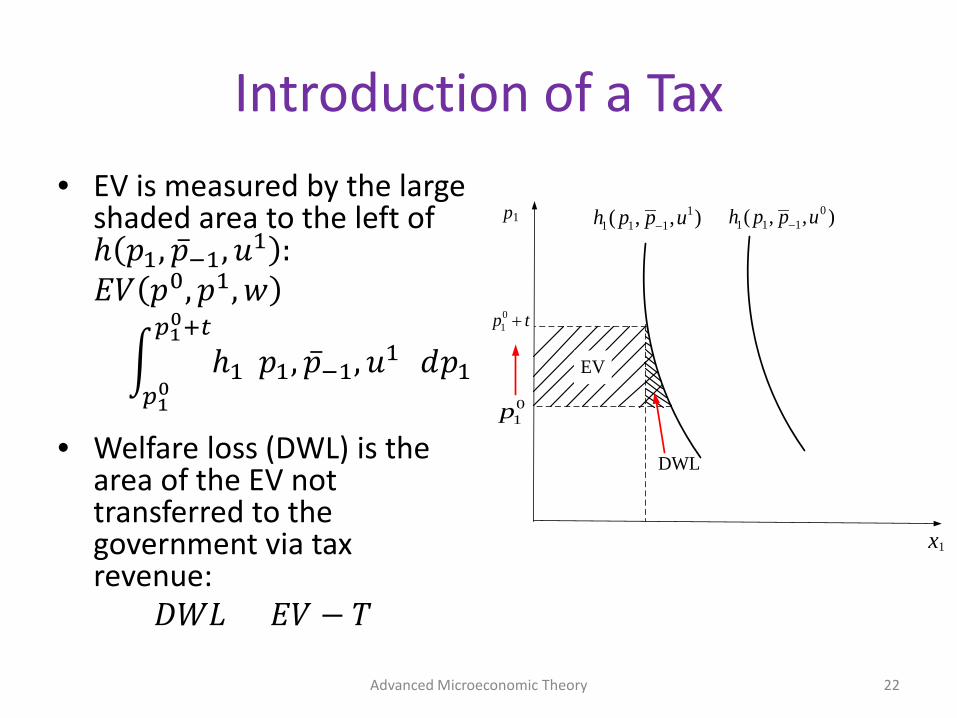
Introduction of a Tax• EV is measured by the large
shaded area to the left of ℎ 𝑝𝑝1, ��𝑝−1, 𝑢𝑢1 :𝐸𝐸𝐶𝐶 𝑝𝑝0, 𝑝𝑝1, 𝑤𝑤
= �𝑝𝑝1
0
𝑝𝑝10+𝑡𝑡
ℎ1(𝑝𝑝1, ��𝑝−1, 𝑢𝑢1) 𝑑𝑑𝑝𝑝1
• Welfare loss (DWL) is the area of the EV not transferred to the government via tax revenue:
𝐷𝐷𝐷𝐷𝐷𝐷 = 𝐸𝐸𝐶𝐶 − 𝑇𝑇
Advanced Microeconomic Theory 22
p1
x1
01p
EV
01 1 1( , , )h p p u−
11 1 1( , , )h p p u−
DWL
01p t+
Why not use the Walrasian demand?
• Walrasian demand is easier to observe, so we could use the variation in consumer’s surplus as an approximation of welfare changes.
• This is only valid when income effects are zero:– Recall that the Walrasian demand measures both
income and substitution effects resulting from a price change, while
– The Hicksian demand measures only substitution effects from such a price change.
• Hence, there will be a difference between CV and CS, and between EV and CS.
Advanced Microeconomic Theory 23
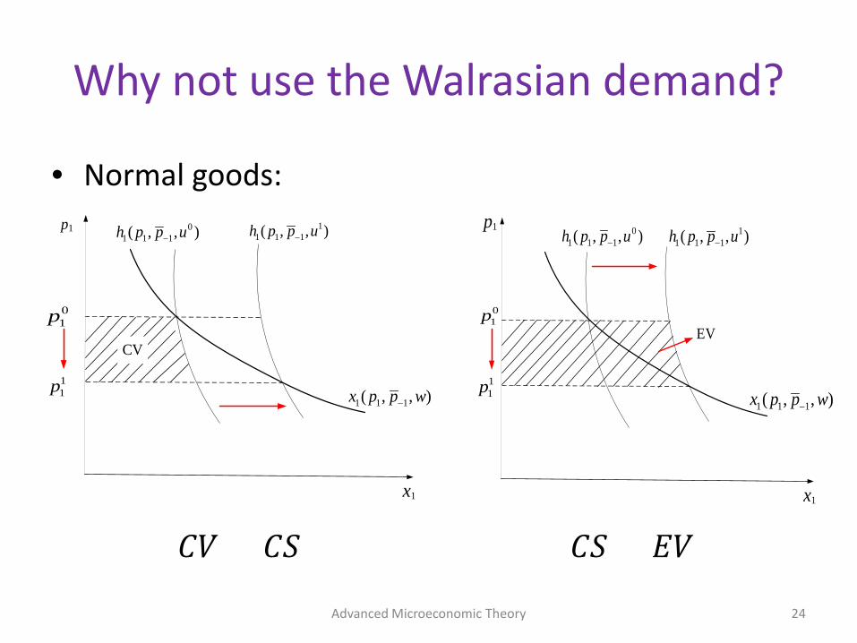
Why not use the Walrasian demand?
• Normal goods:
Advanced Microeconomic Theory 24
𝐶𝐶𝐶𝐶 < 𝐶𝐶𝐶𝐶 𝐶𝐶𝐶𝐶 < 𝐸𝐸𝐶𝐶
p1
x1
01p
11p
CV
01 1 1( , , )h p p u−
11 1 1( , , )h p p u−
1 1 1( , , )x p p w−
x1
01 1 1( , , )h p p u−
11 1 1( , , )h p p u−
1 1 1( , , )x p p w−
p1
EV01p
11p
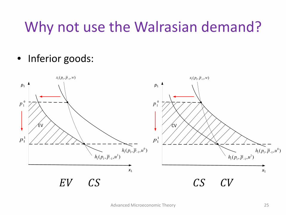
Why not use the Walrasian demand?
• Inferior goods:
Advanced Microeconomic Theory 25
𝐸𝐸𝐶𝐶 < 𝐶𝐶𝐶𝐶 𝐶𝐶𝐶𝐶 < 𝐶𝐶𝐶𝐶
p1
x1
EV
p1
x1
CV
Why not use the Walrasian demand?
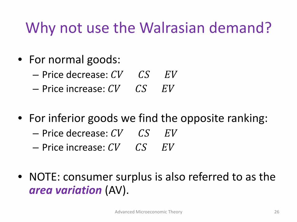
• For normal goods:– Price decrease: 𝐶𝐶𝐶𝐶 < 𝐶𝐶𝐶𝐶 < 𝐸𝐸𝐶𝐶– Price increase: 𝐶𝐶𝐶𝐶 > 𝐶𝐶𝐶𝐶 > 𝐸𝐸𝐶𝐶
• For inferior goods we find the opposite ranking:– Price decrease: 𝐶𝐶𝐶𝐶 > 𝐶𝐶𝐶𝐶 > 𝐸𝐸𝐶𝐶– Price increase: 𝐶𝐶𝐶𝐶 < 𝐶𝐶𝐶𝐶 < 𝐸𝐸𝐶𝐶
• NOTE: consumer surplus is also referred to as the area variation (AV).
Advanced Microeconomic Theory 26
When can we use the Walrasian demand?
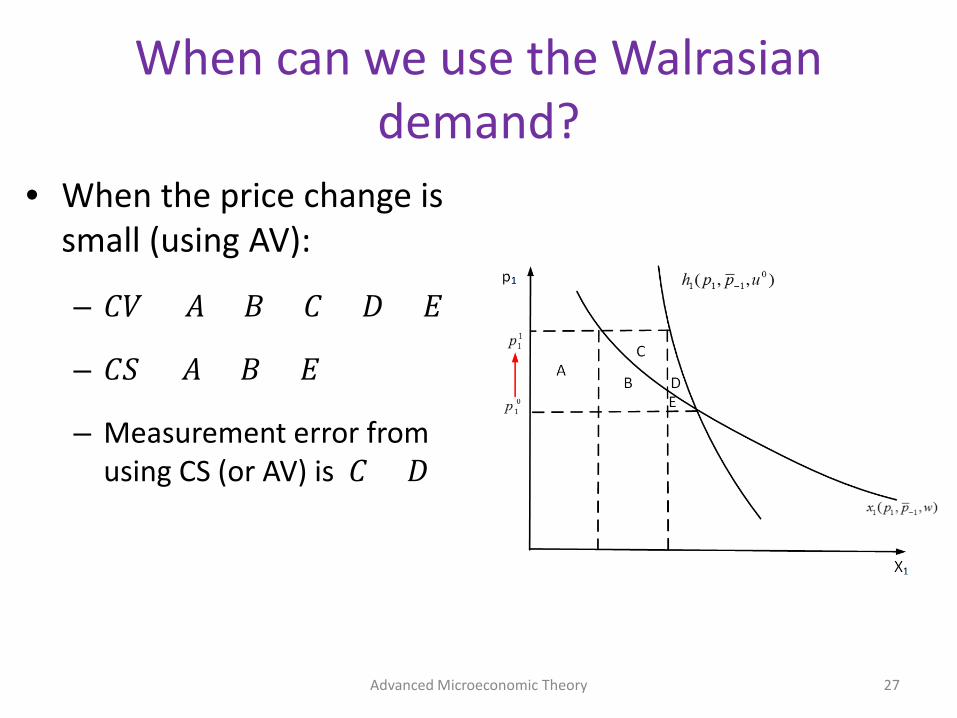
• When the price change is small (using AV):
– 𝐶𝐶𝐶𝐶 = 𝐴𝐴 + 𝐵𝐵 + 𝐶𝐶 + 𝐷𝐷 + 𝐸𝐸
– 𝐶𝐶𝐶𝐶 = 𝐴𝐴 + 𝐵𝐵 + 𝐸𝐸
– Measurement error from using CS (or AV) is 𝐶𝐶 + 𝐷𝐷
Advanced Microeconomic Theory 27
When can we use the Walrasian demand?
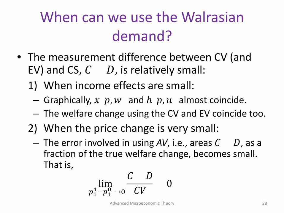
• The measurement difference between CV (and EV) and CS, 𝐶𝐶 + 𝐷𝐷, is relatively small:1) When income effects are small:– Graphically, 𝑥𝑥(𝑝𝑝, 𝑤𝑤) and ℎ(𝑝𝑝, 𝑢𝑢) almost coincide.– The welfare change using the CV and EV coincide too.
2) When the price change is very small:– The error involved in using AV, i.e., areas 𝐶𝐶 + 𝐷𝐷, as a
fraction of the true welfare change, becomes small. That is,
lim(𝑝𝑝1
1−𝑝𝑝10)→0
𝐶𝐶 + 𝐷𝐷𝐶𝐶𝐶𝐶
= 0
Advanced Microeconomic Theory 28
When can we use the Walrasian demand?
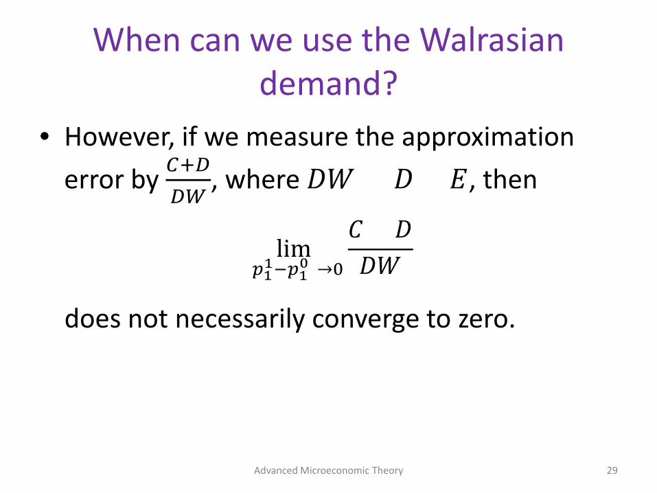
• However, if we measure the approximation error by 𝐶𝐶+𝐷𝐷
𝐷𝐷𝐷𝐷, where 𝐷𝐷𝐷𝐷 = 𝐷𝐷 + 𝐸𝐸, then
lim(𝑝𝑝1
1−𝑝𝑝10)→0
𝐶𝐶 + 𝐷𝐷𝐷𝐷𝐷𝐷
does not necessarily converge to zero.
Advanced Microeconomic Theory 29
When can we use the Walrasian demand?
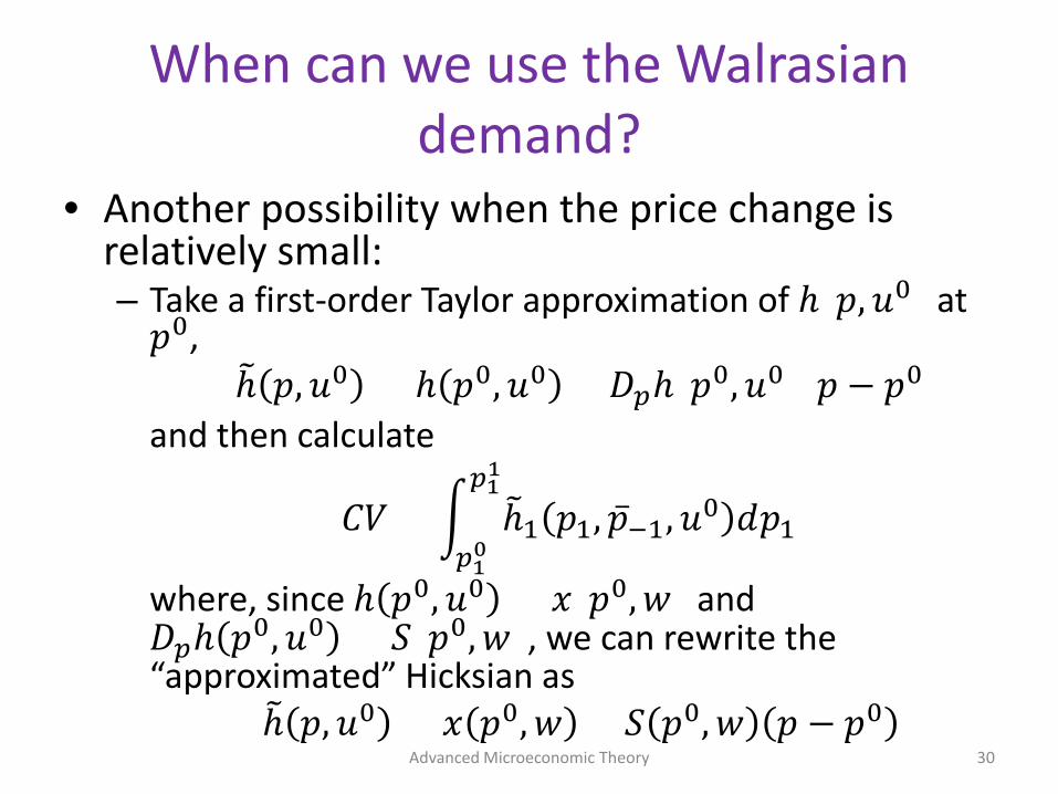
• Another possibility when the price change is relatively small: – Take a first-order Taylor approximation of ℎ(𝑝𝑝, 𝑢𝑢0) at
𝑝𝑝0,�ℎ 𝑝𝑝, 𝑢𝑢0 = ℎ 𝑝𝑝0, 𝑢𝑢0 + 𝐷𝐷𝑝𝑝ℎ(𝑝𝑝0, 𝑢𝑢0)(𝑝𝑝 − 𝑝𝑝0)
and then calculate
𝐶𝐶𝐶𝐶 = �𝑝𝑝1
0
𝑝𝑝11
�ℎ1 𝑝𝑝1, ��𝑝−1, 𝑢𝑢0 𝑑𝑑𝑝𝑝1
where, since ℎ 𝑝𝑝0, 𝑢𝑢0 = 𝑥𝑥(𝑝𝑝0, 𝑤𝑤) and 𝐷𝐷𝑝𝑝ℎ 𝑝𝑝0, 𝑢𝑢0 = 𝐶𝐶(𝑝𝑝0, 𝑤𝑤), we can rewrite the “approximated” Hicksian as
�ℎ 𝑝𝑝, 𝑢𝑢0 = 𝑥𝑥 𝑝𝑝0, 𝑤𝑤 + 𝐶𝐶 𝑝𝑝0, 𝑤𝑤 𝑝𝑝 − 𝑝𝑝0Advanced Microeconomic Theory 30
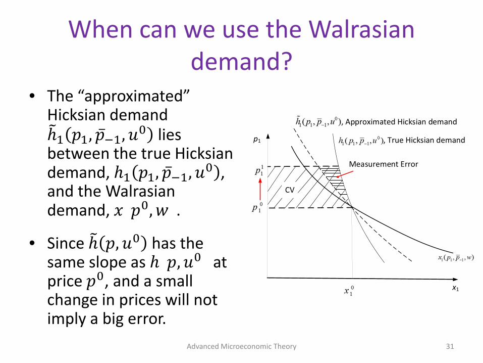
When can we use the Walrasian demand?
• The “approximated” Hicksian demand �ℎ1 𝑝𝑝1, ��𝑝−1, 𝑢𝑢0 lies between the true Hicksian demand, ℎ1 𝑝𝑝1, ��𝑝−1, 𝑢𝑢0 , and the Walrasian demand, 𝑥𝑥(𝑝𝑝0, 𝑤𝑤).
• Since �ℎ 𝑝𝑝, 𝑢𝑢0 has the same slope as ℎ(𝑝𝑝, 𝑢𝑢0) at price 𝑝𝑝0, and a small change in prices will not imply a big error.
Advanced Microeconomic Theory 31
p1
x1
CV
, Approximated Hicksian demand
, True Hicksian demand
Measurement Error
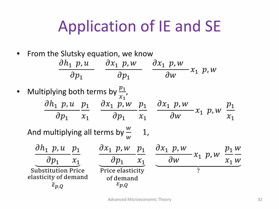
Application of IE and SE• From the Slutsky equation, we know
𝜕𝜕ℎ1(𝑝𝑝, 𝑢𝑢)𝜕𝜕𝑝𝑝1
=𝜕𝜕𝑥𝑥1(𝑝𝑝, 𝑤𝑤)
𝜕𝜕𝑝𝑝1+
𝜕𝜕𝑥𝑥1(𝑝𝑝, 𝑤𝑤)𝜕𝜕𝑤𝑤 𝑥𝑥1(𝑝𝑝, 𝑤𝑤)
• Multiplying both terms by 𝑝𝑝1𝑥𝑥1
,𝜕𝜕ℎ1(𝑝𝑝, 𝑢𝑢)
𝜕𝜕𝑝𝑝1
𝑝𝑝1
𝑥𝑥1=
𝜕𝜕𝑥𝑥1(𝑝𝑝, 𝑤𝑤)𝜕𝜕𝑝𝑝1
𝑝𝑝1
𝑥𝑥1+
𝜕𝜕𝑥𝑥1(𝑝𝑝, 𝑤𝑤)𝜕𝜕𝑤𝑤 𝑥𝑥1(𝑝𝑝, 𝑤𝑤)
𝑝𝑝1
𝑥𝑥1
And multiplying all terms by 𝑤𝑤𝑤𝑤
= 1,
𝜕𝜕ℎ1(𝑝𝑝, 𝑢𝑢)𝜕𝜕𝑝𝑝1
𝑝𝑝1
𝑥𝑥1Substitution Price
elasticity of demand�𝜀𝜀𝑝𝑝,𝑄𝑄
=𝜕𝜕𝑥𝑥1(𝑝𝑝, 𝑤𝑤)
𝜕𝜕𝑝𝑝1
𝑝𝑝1
𝑥𝑥1Price elasticity
of demand𝜀𝜀𝑝𝑝,𝑄𝑄
+𝜕𝜕𝑥𝑥1(𝑝𝑝, 𝑤𝑤)
𝜕𝜕𝑤𝑤 𝑥𝑥1(𝑝𝑝, 𝑤𝑤)𝑝𝑝1
𝑥𝑥1
𝑤𝑤𝑤𝑤
?
Advanced Microeconomic Theory 32
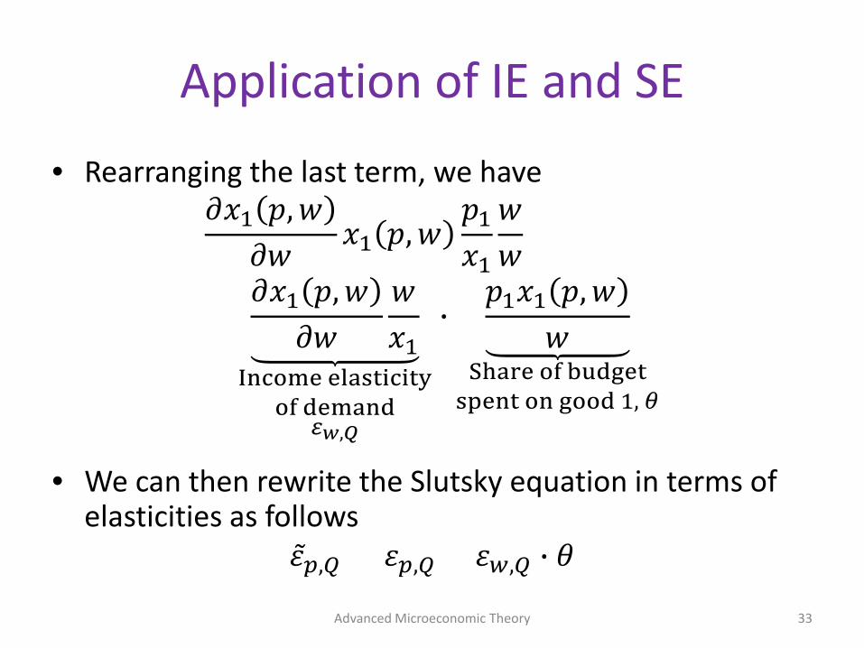
Application of IE and SE
• Rearranging the last term, we have𝜕𝜕𝑥𝑥1 𝑝𝑝, 𝑤𝑤
𝜕𝜕𝑤𝑤𝑥𝑥1 𝑝𝑝, 𝑤𝑤
𝑝𝑝1
𝑥𝑥1
𝑤𝑤𝑤𝑤
=𝜕𝜕𝑥𝑥1 𝑝𝑝, 𝑤𝑤
𝜕𝜕𝑤𝑤𝑤𝑤𝑥𝑥1
Income elasticityof demand
𝜀𝜀𝑤𝑤,𝑄𝑄
�𝑝𝑝1𝑥𝑥1 𝑝𝑝, 𝑤𝑤
𝑤𝑤Share of budget
spent on good 1, 𝜃𝜃
• We can then rewrite the Slutsky equation in terms of elasticities as follows
𝜀𝜀𝑝𝑝,𝑄𝑄 = 𝜀𝜀𝑝𝑝,𝑄𝑄 + 𝜀𝜀𝑤𝑤,𝑄𝑄 � 𝜃𝜃
Advanced Microeconomic Theory 33
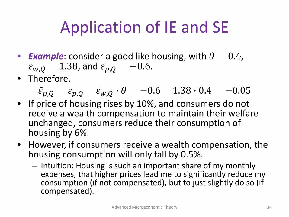
Application of IE and SE• Example: consider a good like housing, with 𝜃𝜃 = 0.4,
𝜀𝜀𝑤𝑤,𝑄𝑄 = 1.38, and 𝜀𝜀𝑝𝑝,𝑄𝑄 = −0.6.• Therefore,
𝜀𝜀𝑝𝑝,𝑄𝑄 = 𝜀𝜀𝑝𝑝,𝑄𝑄 + 𝜀𝜀𝑤𝑤,𝑄𝑄 � 𝜃𝜃 = −0.6 + 1.38 � 0.4 = −0.05• If price of housing rises by 10%, and consumers do not
receive a wealth compensation to maintain their welfare unchanged, consumers reduce their consumption of housing by 6%.
• However, if consumers receive a wealth compensation, the housing consumption will only fall by 0.5%.– Intuition: Housing is such an important share of my monthly
expenses, that higher prices lead me to significantly reduce my consumption (if not compensated), but to just slightly do so (if compensated).
Advanced Microeconomic Theory 34

Application of IE and SE
• Other useful lessons from the previous expression
𝜀𝜀𝑝𝑝,𝑄𝑄 = 𝜀𝜀𝑝𝑝,𝑄𝑄 + 𝜀𝜀𝑤𝑤,𝑄𝑄 � 𝜃𝜃
• Price-elasticities very close 𝜀𝜀𝑝𝑝,𝑄𝑄 ≃ 𝜀𝜀𝑝𝑝,𝑄𝑄 if– Share of budget spent on this particular good, 𝜃𝜃, is
very small (Example: garlic).– The income-elasticity is really small (Example: pizza).
• Advantages if 𝜀𝜀𝑝𝑝,𝑄𝑄 ≃ 𝜀𝜀𝑝𝑝,𝑄𝑄:– The Walrasian and Hicksian demand are very close to
each other. Hence, 𝐶𝐶𝐶𝐶 ≃ 𝐸𝐸𝐶𝐶 ≃ 𝐶𝐶𝐶𝐶.
Advanced Microeconomic Theory 35

Application of IE and SE
• You can read sometimes “in this study we use the change in CS to measure welfare changes due to a price increase given that income effects are negligible”– What the authors are referring to is: Share of budget spent on the good is relatively small and/or The income-elasticity of the good is small
• Remember that our results are not only applicable to price changes, but also to changes in the sales taxes.
• For which preference relations a price change induces no income effect? Quasilinear.
Advanced Microeconomic Theory 36

Application of IE and SE
• In 1981 the US negotiated voluntary automobile export restrictions with the Japanese government.
• Clifford Winston (1987) studied the effects of these export restrictions:– Car prices: 𝑝𝑝𝐽𝐽𝐽𝐽𝑝𝑝 was 20% higher with restrictions that
without. 𝑝𝑝𝑈𝑈𝑈𝑈 was 8% higher with restrictions than without.
– What is the effect of these higher prices on consumer’s welfare?
– Would you use CS? Probably not, since both 𝜃𝜃 and 𝜀𝜀𝑤𝑤,𝑄𝑄 are relatively high.
Advanced Microeconomic Theory 37
Application of IE and SE• Winston did not use CS. Instead, he focused on the CV.
He found that CV = -$14 billion.– Intuition: The wealth compensation that domestic car
owners would need after the price change (after setting the export restrictions) in order to be as well off as they were before the price change is $14 billion.
• This implies that, considering that in 1987 there were 179 million car owners in the US, the wealth compensation per car owner should have been $14,000/$179 = $78.
• Of course, this is an underestimation, since we should divide over the number of new care owners during the period of export restriction was active (not the number of all car owners).
Advanced Microeconomic Theory 38

Application of IE and SE
• Jerry Hausmann (MIT) measures the welfare gain consumers obtain from the price decrease they experience after a Walmart store locates in their locality/country.
• He used CV. Why? Low-income families spend a non-negligible part of their budget in Wal-Mart.
• Result: welfare improvement of 3.75%.
Advanced Microeconomic Theory 39

Consumer as a Labor Supplier
Advanced Microeconomic Theory 40

Consumer as a Labor Supplier
• Consider the following UMP, where the consumer chooses the amount of goods, 𝑥𝑥, and leisure, 𝐷𝐷, that solve
max𝑥𝑥,𝐿𝐿
𝑢𝑢(𝑥𝑥, 𝐷𝐷)
s. t. ∑𝑖𝑖=1𝐾𝐾 𝑝𝑝𝑖𝑖𝑥𝑥𝑖𝑖 ≤ 𝑀𝑀 = 𝑤𝑤𝑤𝑤 + �𝑀𝑀
and 𝑇𝑇 = 𝑤𝑤 + 𝐷𝐷where 𝑀𝑀 is total wealth, coming from the 𝑤𝑤 hours dedicated to work (at a wage 𝑤𝑤 per hour), and the non-work income, �𝑀𝑀. Total time 𝑇𝑇 must be either dedicated to work (𝑤𝑤) or leisure (𝐷𝐷).
Advanced Microeconomic Theory 41
Consumer as a Labor Supplier
• Let us now use the Composite Commodity Theorem:– If the prices for all goods maintain a constant
proportion with respect to the price of labor (wage), i.e., 𝑝𝑝1 = 𝛼𝛼1𝑤𝑤, …, 𝑝𝑝𝑛𝑛 = 𝛼𝛼𝑛𝑛𝑤𝑤, we can represent these goods all by a single (composite) commodity 𝑦𝑦, with price 𝑝𝑝.
– Then, we have only two goods: the composite commodity 𝑦𝑦 and the number of hours dedicated to work, 𝑤𝑤.
Advanced Microeconomic Theory 42
Consumer as a Labor Supplier
• Hence, the UMP can be rewritten as
max𝑦𝑦,𝑧𝑧
𝑣𝑣(𝑦𝑦, 𝑤𝑤)
s. t. 𝑝𝑝𝑦𝑦 ≤ 𝑤𝑤𝑤𝑤 + �𝑀𝑀
where 𝑝𝑝𝑦𝑦 represents the money spent on consumption goods, and 𝑤𝑤𝑤𝑤 + �𝑀𝑀 reflects the total income originating from labor and non-labor sources.
Advanced Microeconomic Theory 43

Consumer as a Labor Supplier
• The Lagrangian of this UMP is𝐷𝐷 = 𝑣𝑣 𝑦𝑦, 𝑤𝑤 + 𝜆𝜆( �𝑀𝑀 + 𝑤𝑤𝑤𝑤 − 𝑝𝑝𝑦𝑦)
and the FOCs (for interior optimum) are𝜕𝜕𝐷𝐷𝜕𝜕𝑦𝑦
= 𝑣𝑣𝑦𝑦 − 𝜆𝜆𝑝𝑝 = 0 ⟹ 𝜆𝜆 =𝑣𝑣𝑦𝑦
𝑝𝑝𝜕𝜕𝐷𝐷𝜕𝜕𝑤𝑤
= 𝑣𝑣𝑧𝑧 + 𝜆𝜆𝑤𝑤 = 0 ⟹ 𝜆𝜆 = −𝑣𝑣𝑧𝑧
𝑤𝑤• Hence,
𝑣𝑣𝑦𝑦
𝑝𝑝= − 𝑣𝑣𝑧𝑧
𝑤𝑤.
– That is, at the optimum the marginal utility per dollar earned working must be equal to the marginal utility per dollar spent on consumption goods.
Advanced Microeconomic Theory 44
Consumer as a Labor Supplier
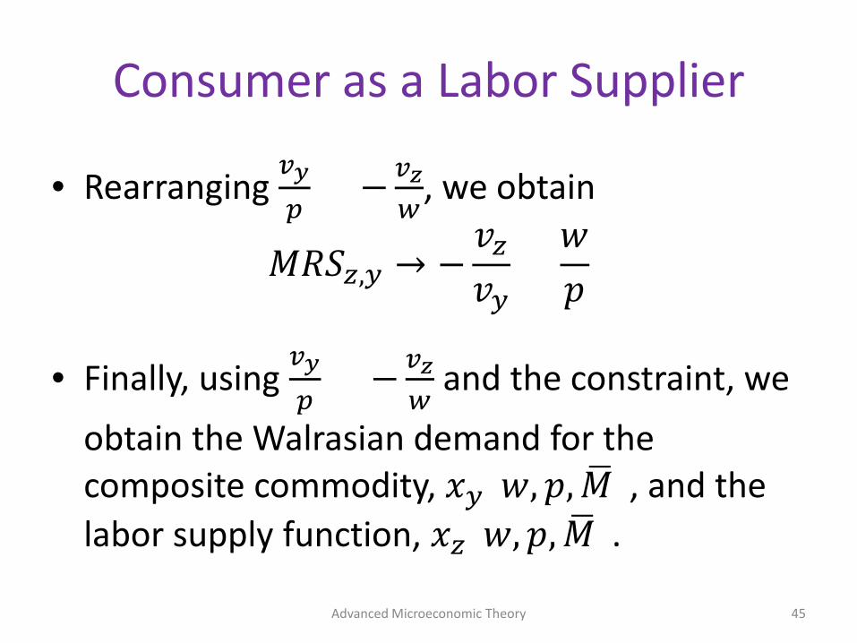
• Rearranging 𝑣𝑣𝑦𝑦
𝑝𝑝= − 𝑣𝑣𝑧𝑧
𝑤𝑤, we obtain
𝑀𝑀𝑀𝑀𝐶𝐶𝑧𝑧,𝑦𝑦 → −𝑣𝑣𝑧𝑧
𝑣𝑣𝑦𝑦=
𝑤𝑤𝑝𝑝
• Finally, using 𝑣𝑣𝑦𝑦
𝑝𝑝= − 𝑣𝑣𝑧𝑧
𝑤𝑤and the constraint, we
obtain the Walrasian demand for the composite commodity, 𝑥𝑥𝑦𝑦(𝑤𝑤, 𝑝𝑝, �𝑀𝑀), and the labor supply function, 𝑥𝑥𝑧𝑧(𝑤𝑤, 𝑝𝑝, �𝑀𝑀).
Advanced Microeconomic Theory 45
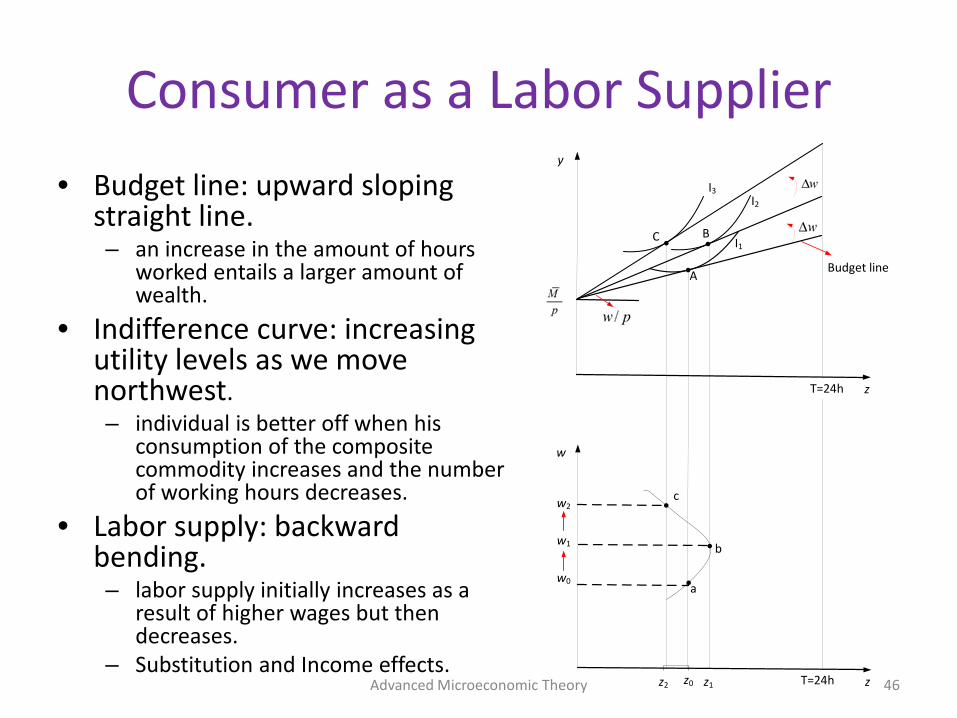
Consumer as a Labor Supplier• Budget line: upward sloping
straight line.– an increase in the amount of hours
worked entails a larger amount of wealth.
• Indifference curve: increasing utility levels as we move northwest. – individual is better off when his
consumption of the composite commodity increases and the number of working hours decreases.
• Labor supply: backward bending.– labor supply initially increases as a
result of higher wages but then decreases.
– Substitution and Income effects.Advanced Microeconomic Theory 46
y
z
w
z
Budget line
w1
w2
w0
z0 z1z2
a
b
c
A
BC I1
I2
I3
T=24h
T=24h
Consumer as a Labor Supplier
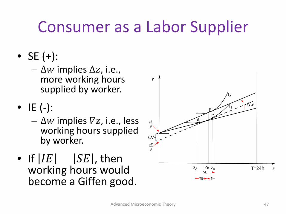
• SE (+): – ∆𝑤𝑤 implies ∆𝑤𝑤, i.e.,
more working hours supplied by worker.
• IE (-): – ∆𝑤𝑤 implies 𝛻𝛻𝑤𝑤, i.e., less
working hours supplied by worker.
• If 𝐼𝐼𝐸𝐸 > 𝐶𝐶𝐸𝐸 , then working hours would become a Giffen good.
Advanced Microeconomic Theory 47
y
zzB zDzA
A
BI1
I2
T=24h
D
CV
Consumer as a Labor Supplier
• How to relate this income and substitution effects with the Slutsky equation?– First, let us state the previous problems as a EMP
min𝑦𝑦,𝑧𝑧
�𝑀𝑀 = 𝑝𝑝𝑦𝑦 − 𝑤𝑤𝑤𝑤
s. t. 𝑣𝑣 𝑦𝑦, 𝑤𝑤 = 𝑣𝑣– From this EMP we can find the optimal hicksian
demands, ℎ𝑦𝑦(𝑤𝑤, 𝑝𝑝, 𝑣𝑣) and ℎ𝑧𝑧 𝑤𝑤, 𝑝𝑝, 𝑣𝑣 .– Inserting them into the objective function, we
obtain the value function of this EMP (i.e., the expenditure function):
𝑒𝑒 𝑤𝑤, 𝑝𝑝, 𝑣𝑣 = 𝑝𝑝ℎ𝑦𝑦 𝑤𝑤, 𝑝𝑝, 𝑣𝑣 + 𝑤𝑤ℎ𝑧𝑧(𝑤𝑤, 𝑝𝑝, 𝑣𝑣)Advanced Microeconomic Theory 48
Consumer as a Labor Supplier
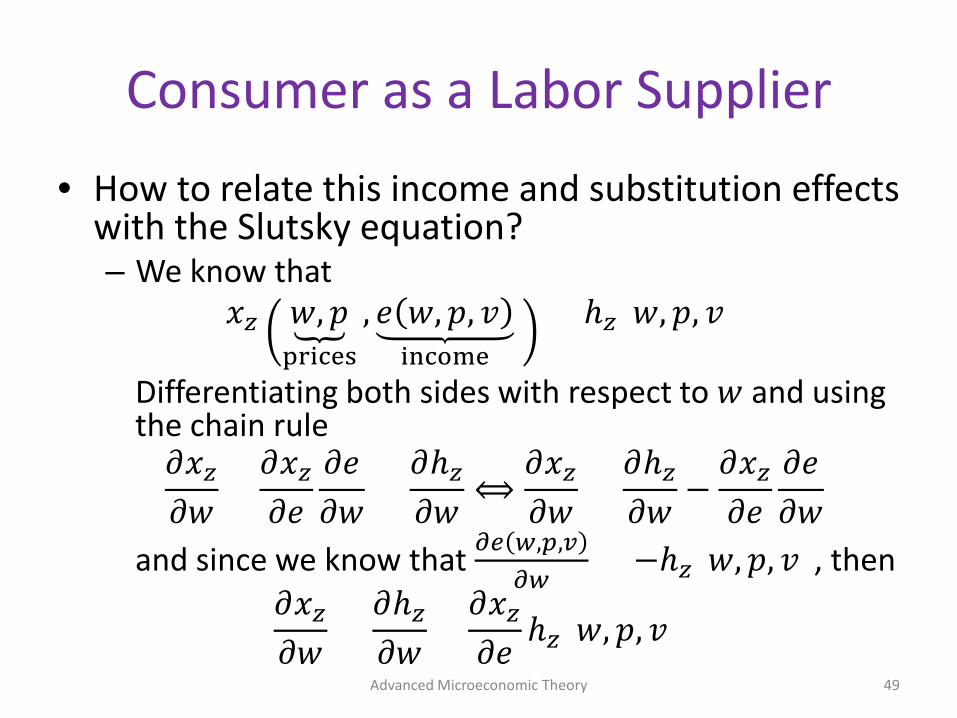
• How to relate this income and substitution effects with the Slutsky equation?– We know that
𝑥𝑥𝑧𝑧 �𝑤𝑤, 𝑝𝑝prices
, 𝑒𝑒 𝑤𝑤, 𝑝𝑝, 𝑣𝑣income
= ℎ𝑧𝑧(𝑤𝑤, 𝑝𝑝, 𝑣𝑣)
Differentiating both sides with respect to 𝑤𝑤 and using the chain rule
𝜕𝜕𝑥𝑥𝑧𝑧
𝜕𝜕𝑤𝑤+
𝜕𝜕𝑥𝑥𝑧𝑧
𝜕𝜕𝑒𝑒𝜕𝜕𝑒𝑒𝜕𝜕𝑤𝑤
=𝜕𝜕ℎ𝑧𝑧
𝜕𝜕𝑤𝑤⟺
𝜕𝜕𝑥𝑥𝑧𝑧
𝜕𝜕𝑤𝑤=
𝜕𝜕ℎ𝑧𝑧
𝜕𝜕𝑤𝑤−
𝜕𝜕𝑥𝑥𝑧𝑧
𝜕𝜕𝑒𝑒𝜕𝜕𝑒𝑒𝜕𝜕𝑤𝑤
and since we know that 𝜕𝜕𝑒𝑒 𝑤𝑤,𝑝𝑝,𝑣𝑣𝜕𝜕𝑤𝑤
= −ℎ𝑧𝑧(𝑤𝑤, 𝑝𝑝, 𝑣𝑣), then 𝜕𝜕𝑥𝑥𝑧𝑧
𝜕𝜕𝑤𝑤=
𝜕𝜕ℎ𝑧𝑧
𝜕𝜕𝑤𝑤+
𝜕𝜕𝑥𝑥𝑧𝑧
𝜕𝜕𝑒𝑒ℎ𝑧𝑧(𝑤𝑤, 𝑝𝑝, 𝑣𝑣)
Advanced Microeconomic Theory 49
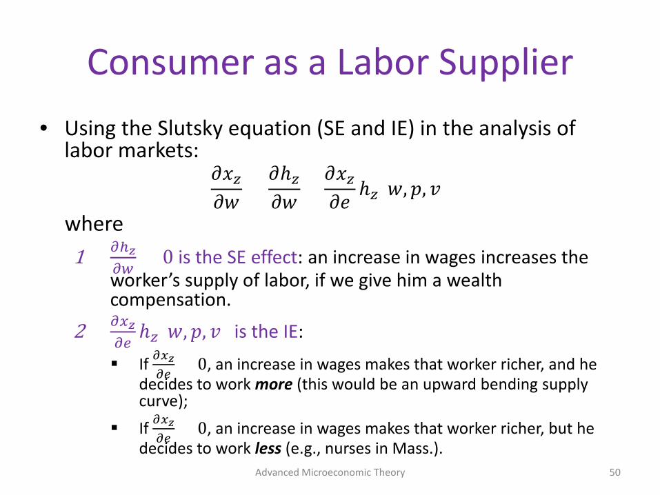
Consumer as a Labor Supplier• Using the Slutsky equation (SE and IE) in the analysis of
labor markets:𝜕𝜕𝑥𝑥𝑧𝑧
𝜕𝜕𝑤𝑤 =𝜕𝜕ℎ𝑧𝑧
𝜕𝜕𝑤𝑤 +𝜕𝜕𝑥𝑥𝑧𝑧
𝜕𝜕𝑒𝑒 ℎ𝑧𝑧(𝑤𝑤, 𝑝𝑝, 𝑣𝑣)
where1) 𝜕𝜕ℎ𝑧𝑧
𝜕𝜕𝑤𝑤> 0 is the SE effect: an increase in wages increases the
worker’s supply of labor, if we give him a wealth compensation.
2) 𝜕𝜕𝑥𝑥𝑧𝑧𝜕𝜕𝑒𝑒
ℎ𝑧𝑧(𝑤𝑤, 𝑝𝑝, 𝑣𝑣) is the IE:
If 𝜕𝜕𝑥𝑥𝑧𝑧𝜕𝜕𝑒𝑒
> 0, an increase in wages makes that worker richer, and he decides to work more (this would be an upward bending supply curve);
If 𝜕𝜕𝑥𝑥𝑧𝑧𝜕𝜕𝑒𝑒
< 0, an increase in wages makes that worker richer, but he decides to work less (e.g., nurses in Mass.).
Advanced Microeconomic Theory 50
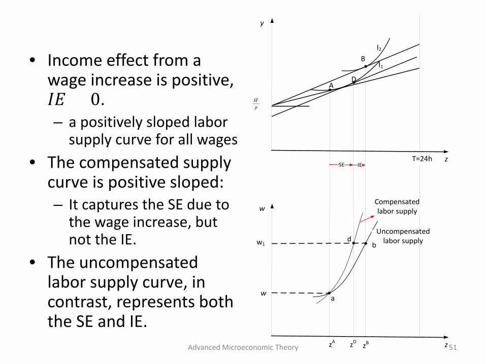
• Income effect from a wage increase is positive, 𝐼𝐼𝐸𝐸 > 0.– a positively sloped labor
supply curve for all wages• The compensated supply
curve is positive sloped:– It captures the SE due to
the wage increase, but not the IE.
• The uncompensated labor supply curve, in contrast, represents both the SE and IE.
Advanced Microeconomic Theory 51
y
z
A
BI1
I2
T=24h
D
w
z
w1
w
zBzDzA
a
db
Compensated labor supply
Uncompensated labor supply
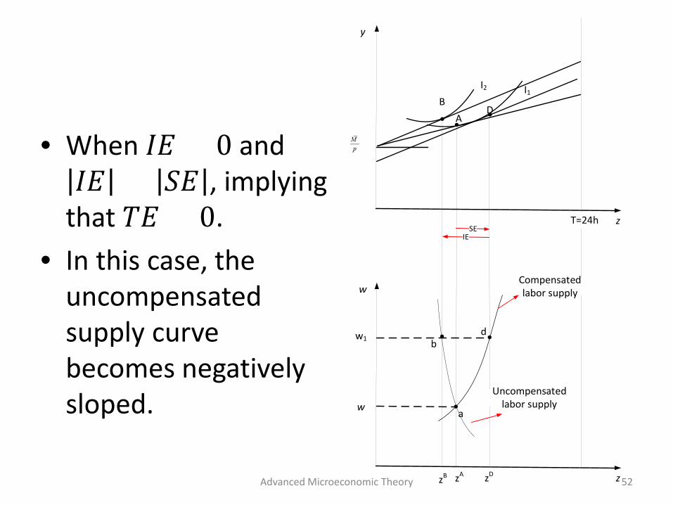
• When 𝐼𝐼𝐸𝐸 < 0 and 𝐼𝐼𝐸𝐸 > 𝐶𝐶𝐸𝐸 , implying
that 𝑇𝑇𝐸𝐸 < 0. • In this case, the
uncompensated supply curve becomes negatively sloped.
Advanced Microeconomic Theory 52
y
z
AB
I1I2
T=24h
D
w
z
w1
w
zB zDzA
a
db
Compensated labor supply
Uncompensated labor supply
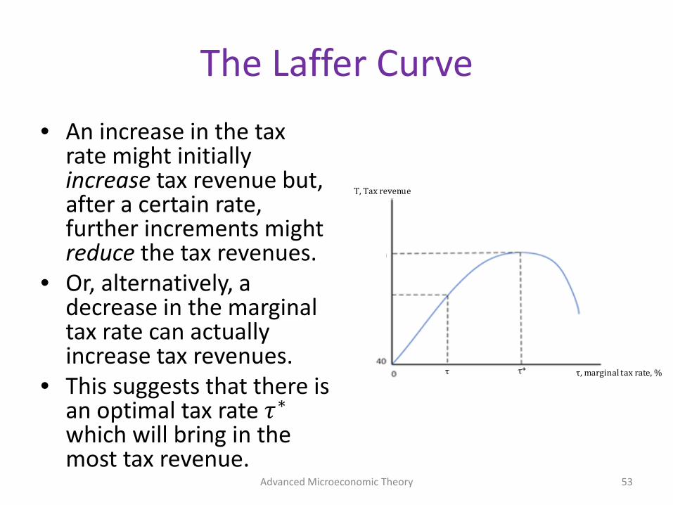
The Laffer Curve• An increase in the tax
rate might initially increase tax revenue but, after a certain rate, further increments might reduce the tax revenues.
• Or, alternatively, a decrease in the marginal tax rate can actually increase tax revenues.
• This suggests that there is an optimal tax rate 𝜏𝜏∗
which will bring in the most tax revenue.
Advanced Microeconomic Theory 53
τ τ* τ, marginal tax rate, %
T, Tax revenue
Consumer as a Labor Supplier
• Consider salary 𝑤𝑤 per hour, and a net salary of 𝜔𝜔 = 1 − 𝜏𝜏 𝑤𝑤
after taxes. • Hence, 𝐻𝐻(𝜔𝜔) represents the number of working
hours, where workers consider their net wage when deciding how many hours to work.
• Therefore, tax revenue is𝑇𝑇 = 𝜏𝜏 � 𝑤𝑤 � 𝐻𝐻(𝜔𝜔)
Advanced Microeconomic Theory 54

Consumer as a Labor Supplier• Since total tax revenue is 𝑇𝑇 = 𝜏𝜏 � 𝑤𝑤 � 𝐻𝐻(𝜔𝜔), the effect of marginally
increasing the tax rate is
𝜕𝜕𝑇𝑇𝜕𝜕𝜏𝜏
= 𝑤𝑤 � 𝐻𝐻 𝜔𝜔 + 𝜏𝜏 � 𝑤𝑤 � (−𝑤𝑤)𝜕𝜕𝐻𝐻𝜕𝜕𝜔𝜔
= 𝑤𝑤 � 𝐻𝐻(𝜔𝜔)Positive effect
− 𝜏𝜏 � 𝑤𝑤2�𝜕𝜕𝐻𝐻𝜕𝜕𝜔𝜔
Negative effect
– The positive effect represents that, for a given supply of working hours, an increase in the tax rate increases tax revenue.
– The negative effect represents that an increase in the tax rate reduces
the amount of working hours supplied and, hence, tax revenue.
Advanced Microeconomic Theory 55
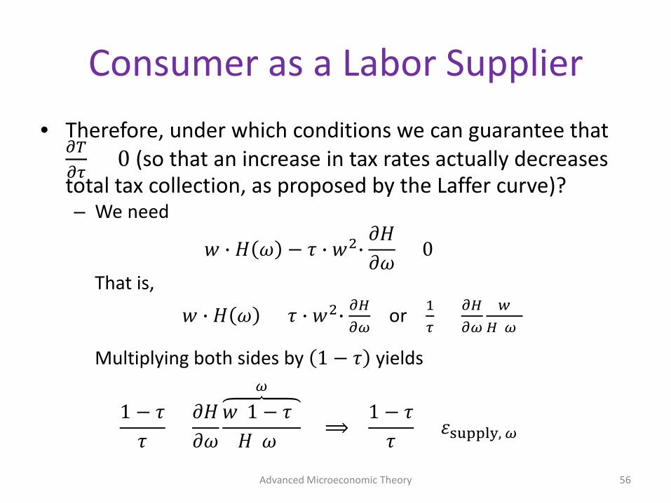
Consumer as a Labor Supplier• Therefore, under which conditions we can guarantee that
𝜕𝜕𝜕𝜕𝜕𝜕𝜕𝜕
< 0 (so that an increase in tax rates actually decreases total tax collection, as proposed by the Laffer curve)?– We need
𝑤𝑤 � 𝐻𝐻 𝜔𝜔 − 𝜏𝜏 � 𝑤𝑤2�𝜕𝜕𝐻𝐻𝜕𝜕𝜔𝜔 < 0
That is,
𝑤𝑤 � 𝐻𝐻 𝜔𝜔 < 𝜏𝜏 � 𝑤𝑤2� 𝜕𝜕𝜕𝜕𝜕𝜕𝜕𝜕
or 1𝜕𝜕
< 𝜕𝜕𝜕𝜕𝜕𝜕𝜕𝜕
𝑤𝑤𝜕𝜕(𝜕𝜕)
Multiplying both sides by 1 − 𝜏𝜏 yields
1 − 𝜏𝜏𝜏𝜏 <
𝜕𝜕𝐻𝐻𝜕𝜕𝜔𝜔
𝑤𝑤(1 − 𝜏𝜏)𝜕𝜕
𝐻𝐻(𝜔𝜔) ⟹1 − 𝜏𝜏
𝜏𝜏 < 𝜀𝜀supply, 𝜕𝜕
Advanced Microeconomic Theory 56

Consumer as a Labor Supplier
• The area above (below) cutoff 1−𝜕𝜕
𝜕𝜕represents
combinations of the elasticity of labor supply (𝜀𝜀supply, 𝜕𝜕) and tax rates (𝜏𝜏) for which a marginal increase in the tax rate yields a smaller (larger, respectively) total tax revenue.
Advanced Microeconomic Theory 57
10.50
1
τ
εsupply,w
1− τ τ
εsupply,w >
1− τ τ
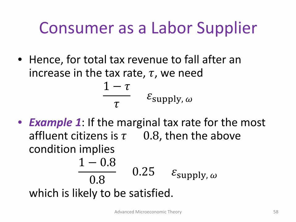
Consumer as a Labor Supplier
• Hence, for total tax revenue to fall after an increase in the tax rate, 𝜏𝜏, we need
1 − 𝜏𝜏𝜏𝜏
< 𝜀𝜀supply, 𝜕𝜕
• Example 1: If the marginal tax rate for the most affluent citizens is 𝜏𝜏 = 0.8, then the above condition implies
1 − 0.80.8
= 0.25 < 𝜀𝜀supply, 𝜕𝜕
which is likely to be satisfied.Advanced Microeconomic Theory 58

Consumer as a Labor Supplier
• Example 2: An economy in which the maximum marginal tax rate is 𝜏𝜏 = 0.35, would need
1 − 0.350.35
= 1.85 < 𝜀𝜀supply, 𝜕𝜕
for total tax revenue to increase, which is very unlikely to hold for the average worker in most developed countries.
Advanced Microeconomic Theory 59

Gross/Net Complements and Gross/Net Substitutes
Advanced Microeconomic Theory 60

Demand Relationships among Goods
• So far, we were focusing on the SE and IE of varying the price of good 𝑘𝑘 on the demand for good 𝑘𝑘.
• Now, we analyze the SE and IE of varying the price of good 𝑘𝑘 on the demand for other good 𝑗𝑗.
Advanced Microeconomic Theory 61
Demand Relationships among Goods
• For simplicity, let us start our analysis with the two-good case. – This will help us graphically illustrate the main
intuitions.
• Later on we generalize our analysis to 𝑁𝑁 > 2goods.
Advanced Microeconomic Theory 62
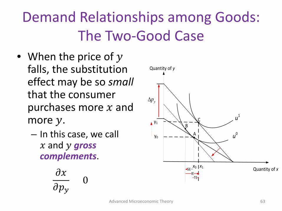
Demand Relationships among Goods: The Two-Good Case
• When the price of 𝑦𝑦falls, the substitution effect may be so smallthat the consumer purchases more 𝑥𝑥 and more 𝑦𝑦.– In this case, we call
𝑥𝑥 and 𝑦𝑦 gross complements.
𝜕𝜕𝑥𝑥𝜕𝜕𝑝𝑝𝑦𝑦
< 0
Advanced Microeconomic Theory 63
Quantity of y
Quantity of x
u1
u0AB
C
x1x0
y0
y1
SE
TE
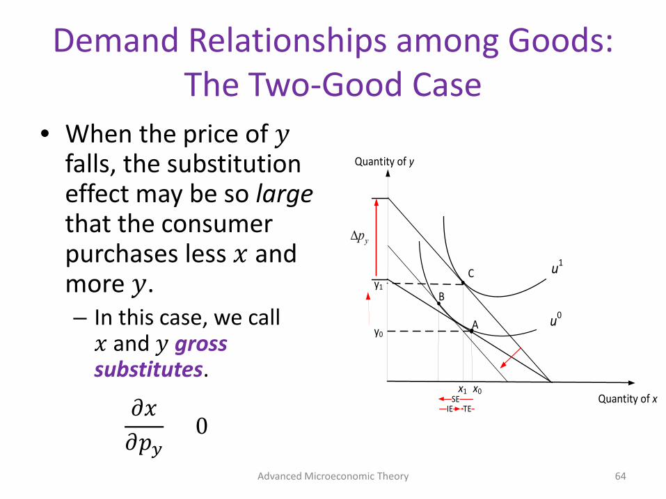
Demand Relationships among Goods: The Two-Good Case
• When the price of 𝑦𝑦falls, the substitution effect may be so largethat the consumer purchases less 𝑥𝑥 and more 𝑦𝑦.– In this case, we call
𝑥𝑥 and 𝑦𝑦 gross substitutes.
𝜕𝜕𝑥𝑥𝜕𝜕𝑝𝑝𝑦𝑦
> 0
Advanced Microeconomic Theory 64
Quantity of y
Quantity of x
u1
u0A
B
C
x1 x0
y0
y1
IE TE
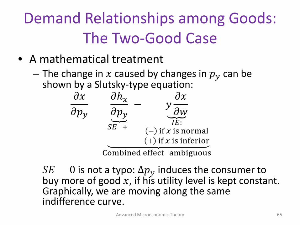
Demand Relationships among Goods: The Two-Good Case
• A mathematical treatment– The change in 𝑥𝑥 caused by changes in 𝑝𝑝𝑦𝑦 can be
shown by a Slutsky-type equation:𝜕𝜕𝑥𝑥
𝜕𝜕𝑝𝑝𝑦𝑦=
�𝜕𝜕ℎ𝑥𝑥
𝜕𝜕𝑝𝑝𝑦𝑦𝑈𝑈𝑆𝑆 (+)
− �𝑦𝑦𝜕𝜕𝑥𝑥𝜕𝜕𝑤𝑤
𝐼𝐼𝑆𝑆:− if 𝑥𝑥 is normal+ if 𝑥𝑥 is inferior
Combined effect (ambiguous)
𝐶𝐶𝐸𝐸 > 0 is not a typo: ∆𝑝𝑝𝑦𝑦 induces the consumer to buy more of good 𝑥𝑥, if his utility level is kept constant. Graphically, we are moving along the same indifference curve.
Advanced Microeconomic Theory 65
Demand Relationships among Goods: The Two-Good Case
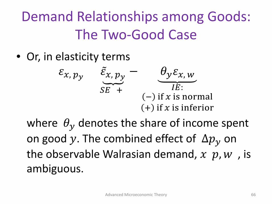
• Or, in elasticity terms𝜀𝜀𝑥𝑥, 𝑝𝑝𝑦𝑦 = �𝜀𝜀𝑥𝑥, 𝑝𝑝𝑦𝑦
𝑈𝑈𝑆𝑆 (+)
− 𝜃𝜃𝑦𝑦𝜀𝜀𝑥𝑥, 𝑤𝑤𝐼𝐼𝑆𝑆:
− if 𝑥𝑥 is normal+ if 𝑥𝑥 is inferior
where 𝜃𝜃𝑦𝑦 denotes the share of income spent on good 𝑦𝑦. The combined effect of ∆𝑝𝑝𝑦𝑦 on the observable Walrasian demand, 𝑥𝑥(𝑝𝑝, 𝑤𝑤), is ambiguous.
Advanced Microeconomic Theory 66
Demand Relationships among Goods: The Two-Good Case
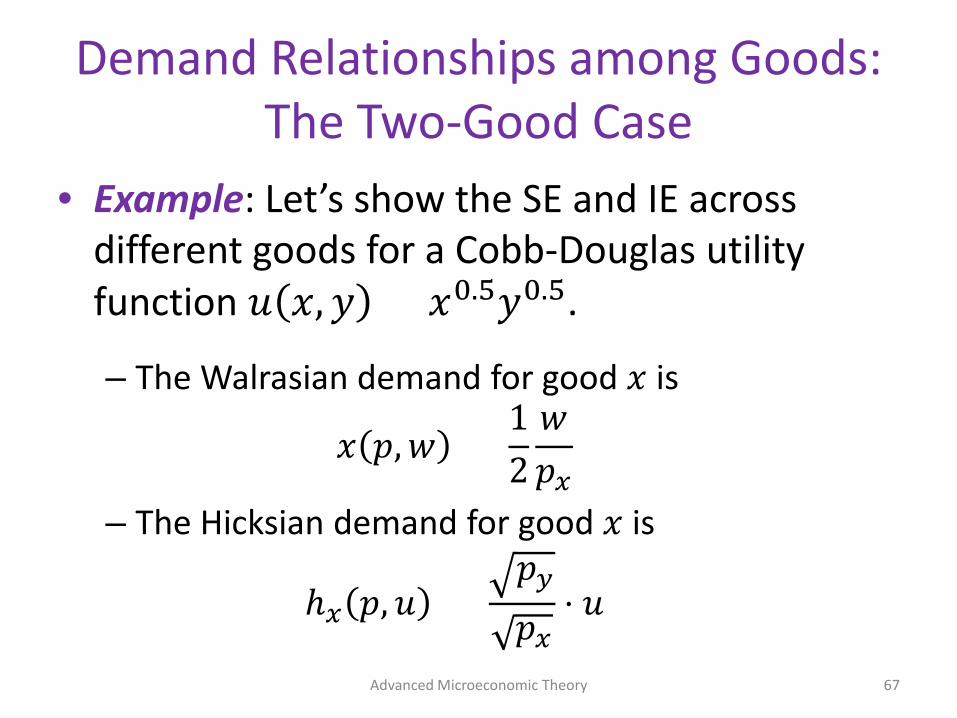
• Example: Let’s show the SE and IE across different goods for a Cobb-Douglas utility function 𝑢𝑢 𝑥𝑥, 𝑦𝑦 = 𝑥𝑥0.5𝑦𝑦0.5.
– The Walrasian demand for good 𝑥𝑥 is
𝑥𝑥 𝑝𝑝, 𝑤𝑤 =12
𝑤𝑤𝑝𝑝𝑥𝑥
– The Hicksian demand for good 𝑥𝑥 is
ℎ𝑥𝑥 𝑝𝑝, 𝑢𝑢 =𝑝𝑝𝑦𝑦
𝑝𝑝𝑥𝑥⋅ 𝑢𝑢
Advanced Microeconomic Theory 67
Demand Relationships among Goods: The Two-Good Case
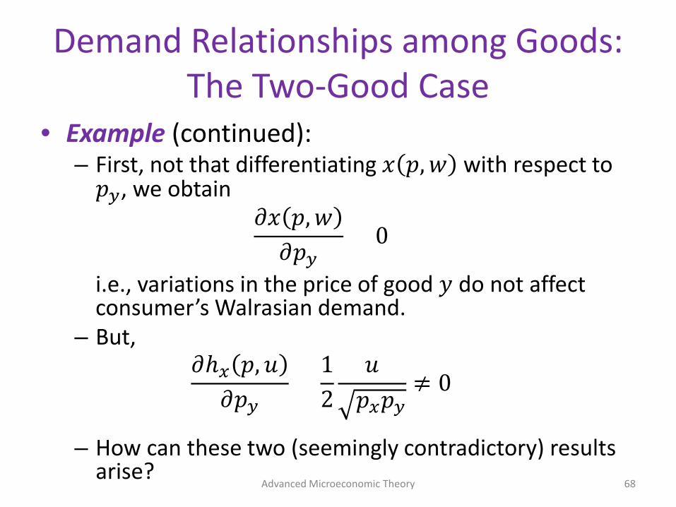
• Example (continued):– First, not that differentiating 𝑥𝑥 𝑝𝑝, 𝑤𝑤 with respect to
𝑝𝑝𝑦𝑦, we obtain𝜕𝜕𝑥𝑥 𝑝𝑝, 𝑤𝑤
𝜕𝜕𝑝𝑝𝑦𝑦= 0
i.e., variations in the price of good 𝑦𝑦 do not affect consumer’s Walrasian demand.
– But,𝜕𝜕ℎ𝑥𝑥 𝑝𝑝, 𝑢𝑢
𝜕𝜕𝑝𝑝𝑦𝑦=
12
𝑢𝑢𝑝𝑝𝑥𝑥𝑝𝑝𝑦𝑦
≠ 0
– How can these two (seemingly contradictory) results arise?
Advanced Microeconomic Theory 68
Demand Relationships among Goods: The Two-Good Case
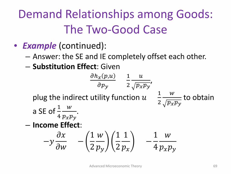
• Example (continued):– Answer: the SE and IE completely offset each other.– Substitution Effect: Given
𝜕𝜕ℎ𝑥𝑥 𝑝𝑝,𝑢𝑢𝜕𝜕𝑝𝑝𝑦𝑦
= 12
𝑢𝑢𝑝𝑝𝑥𝑥𝑝𝑝𝑦𝑦
,
plug the indirect utility function 𝑢𝑢 = 12
𝑤𝑤𝑝𝑝𝑥𝑥𝑝𝑝𝑦𝑦
to obtain
a SE of 14
𝑤𝑤𝑝𝑝𝑥𝑥𝑝𝑝𝑦𝑦
.
– Income Effect:
−𝑦𝑦𝜕𝜕𝑥𝑥𝜕𝜕𝑤𝑤
= −12
𝑤𝑤𝑝𝑝𝑦𝑦
12
1𝑝𝑝𝑥𝑥
= −14
𝑤𝑤𝑝𝑝𝑥𝑥𝑝𝑝𝑦𝑦
Advanced Microeconomic Theory 69
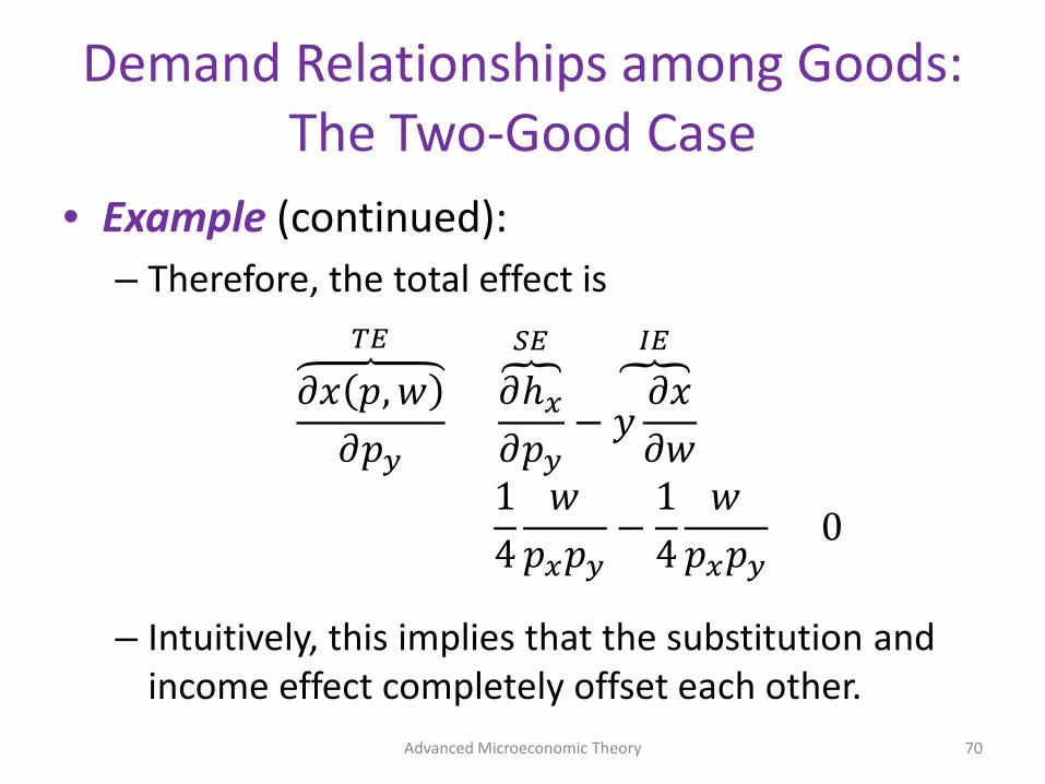
Demand Relationships among Goods: The Two-Good Case
• Example (continued):– Therefore, the total effect is
𝜕𝜕𝑥𝑥 𝑝𝑝, 𝑤𝑤𝜕𝜕𝑝𝑝𝑦𝑦
𝜕𝜕𝑆𝑆
=�𝜕𝜕ℎ𝑥𝑥
𝜕𝜕𝑝𝑝𝑦𝑦
𝑈𝑈𝑆𝑆
−�𝑦𝑦
𝜕𝜕𝑥𝑥𝜕𝜕𝑤𝑤
𝐼𝐼𝑆𝑆
=14
𝑤𝑤𝑝𝑝𝑥𝑥𝑝𝑝𝑦𝑦
−14
𝑤𝑤𝑝𝑝𝑥𝑥𝑝𝑝𝑦𝑦
= 0
– Intuitively, this implies that the substitution and income effect completely offset each other.
Advanced Microeconomic Theory 70
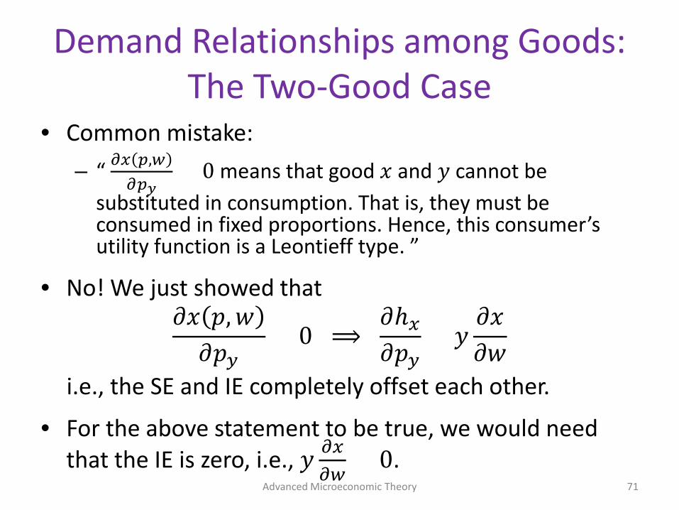
Demand Relationships among Goods: The Two-Good Case
• Common mistake:– “ 𝜕𝜕𝑥𝑥 𝑝𝑝,𝑤𝑤
𝜕𝜕𝑝𝑝𝑦𝑦= 0 means that good 𝑥𝑥 and 𝑦𝑦 cannot be
substituted in consumption. That is, they must be consumed in fixed proportions. Hence, this consumer’s utility function is a Leontieff type. ”
• No! We just showed that𝜕𝜕𝑥𝑥 𝑝𝑝, 𝑤𝑤
𝜕𝜕𝑝𝑝𝑦𝑦= 0 ⟹
𝜕𝜕ℎ𝑥𝑥
𝜕𝜕𝑝𝑝𝑦𝑦= 𝑦𝑦
𝜕𝜕𝑥𝑥𝜕𝜕𝑤𝑤
i.e., the SE and IE completely offset each other.
• For the above statement to be true, we would need that the IE is zero, i.e., 𝑦𝑦 𝜕𝜕𝑥𝑥
𝜕𝜕𝑤𝑤= 0.
Advanced Microeconomic Theory 71
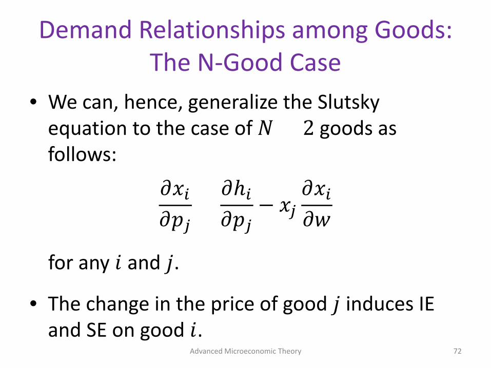
Demand Relationships among Goods: The N-Good Case
• We can, hence, generalize the Slutsky equation to the case of 𝑁𝑁 > 2 goods as follows:
𝜕𝜕𝑥𝑥𝑖𝑖
𝜕𝜕𝑝𝑝𝑗𝑗=
𝜕𝜕ℎ𝑖𝑖
𝜕𝜕𝑝𝑝𝑗𝑗− 𝑥𝑥𝑗𝑗
𝜕𝜕𝑥𝑥𝑖𝑖
𝜕𝜕𝑤𝑤
for any 𝑖𝑖 and 𝑗𝑗.
• The change in the price of good 𝑗𝑗 induces IE and SE on good 𝑖𝑖.
Advanced Microeconomic Theory 72
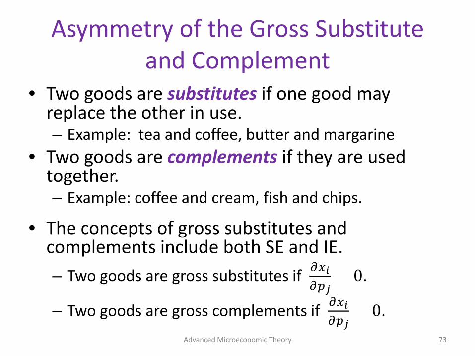
Asymmetry of the Gross Substitute and Complement
• Two goods are substitutes if one good may replace the other in use.– Example: tea and coffee, butter and margarine
• Two goods are complements if they are used together.– Example: coffee and cream, fish and chips.
• The concepts of gross substitutes and complements include both SE and IE.– Two goods are gross substitutes if 𝜕𝜕𝑥𝑥𝑖𝑖
𝜕𝜕𝑝𝑝𝑗𝑗> 0.
– Two goods are gross complements if 𝜕𝜕𝑥𝑥𝑖𝑖𝜕𝜕𝑝𝑝𝑗𝑗
< 0.Advanced Microeconomic Theory 73
Asymmetry of the Gross Substitute and Complement
• The definitions of gross substitutes and complements are not necessarily symmetric.– It is possible for 𝑥𝑥1 to be a substitute for 𝑥𝑥2 and at
the same time for 𝑥𝑥2 to be a complement of 𝑥𝑥1.
• Let us see this potential asymmetry with an example.
Advanced Microeconomic Theory 74
Asymmetry of the Gross Substitute and Complement
• Suppose that the utility function for two goods is given by𝑈𝑈 𝑥𝑥, 𝑦𝑦 = ln 𝑥𝑥 + 𝑦𝑦
• The Lagrangian of the UMP is𝐷𝐷 = ln 𝑥𝑥 + 𝑦𝑦 + 𝜆𝜆(𝑤𝑤 − 𝑝𝑝𝑥𝑥𝑥𝑥 − 𝑝𝑝𝑦𝑦𝑦𝑦)
• The first order conditions are𝜕𝜕𝐷𝐷𝜕𝜕𝑥𝑥
=1𝑥𝑥
− 𝜆𝜆𝑝𝑝𝑥𝑥 = 0𝜕𝜕𝐷𝐷𝜕𝜕𝑦𝑦
= 𝑦𝑦 − 𝜆𝜆𝑝𝑝𝑦𝑦 = 0
𝜕𝜕𝐷𝐷𝜕𝜕𝜆𝜆
= 𝑤𝑤 − 𝑝𝑝𝑥𝑥𝑥𝑥 − 𝑝𝑝𝑦𝑦𝑦𝑦 = 0
Advanced Microeconomic Theory 75
Asymmetry of the Gross Substitute and Complement
• Manipulating the first two equations, we get1
𝑝𝑝𝑥𝑥𝑥𝑥=
1𝑝𝑝𝑦𝑦
⟹ 𝑝𝑝𝑥𝑥𝑥𝑥 = 𝑝𝑝𝑦𝑦
• Inserting this into the budget constraint, we can find the Marshallian demand for 𝑦𝑦
�𝑝𝑝𝑥𝑥𝑥𝑥𝑝𝑝𝑦𝑦
+ 𝑝𝑝𝑦𝑦𝑦𝑦 = 𝑤𝑤 ⟹ 𝑝𝑝𝑦𝑦𝑦𝑦 = 𝑤𝑤 − 𝑝𝑝𝑦𝑦 ⟹
𝑦𝑦 =𝑤𝑤 − 𝑝𝑝𝑦𝑦
𝑝𝑝𝑦𝑦Advanced Microeconomic Theory 76
Asymmetry of the Gross Substitute and Complement
• An increase in 𝑝𝑝𝑦𝑦 causes a decline in spending on 𝑦𝑦– Since 𝑝𝑝𝑥𝑥 and 𝑤𝑤 are unchanged, spending on 𝑥𝑥 must
rise 𝜕𝜕𝑥𝑥𝜕𝜕𝑝𝑝𝑦𝑦
> 0 . Hence, 𝑥𝑥 and 𝑦𝑦 are gross substitutes.
– But spending on 𝑦𝑦 is independent of 𝑝𝑝𝑥𝑥𝜕𝜕𝑦𝑦
𝜕𝜕𝑝𝑝𝑥𝑥= 0 .
Thus, 𝑥𝑥 and 𝑦𝑦 are neither gross substitutes nor gross complements.
– This shows the asymmetry of gross substitute and complement definitions. While good 𝑦𝑦 is a gross substitute of 𝑥𝑥, good 𝑥𝑥 is neither a
gross substitute or complement of 𝑦𝑦.Advanced Microeconomic Theory 77

Asymmetry of the Gross Substitute and Complement
• Depending on how we check for gross substitutability or complementarities between two goods, there is potential to obtain different results.
• Can we use an alternative approach to check if two goods are complements or substitutes in consumption?– Yes. We next present such approach.
Advanced Microeconomic Theory 78

Net Substitutes and Net Complements
• The concepts of net substitutes and complements focus solely on SE. – Two goods are net (or Hicksian) substitutes if
𝜕𝜕ℎ𝑖𝑖
𝜕𝜕𝑝𝑝𝑗𝑗> 0
– Two goods are net (or Hicksian) complements if𝜕𝜕ℎ𝑖𝑖
𝜕𝜕𝑝𝑝𝑗𝑗< 0
where ℎ𝑖𝑖(𝑝𝑝𝑖𝑖 , 𝑝𝑝𝑗𝑗 , 𝑢𝑢) is the Hicksian demand of good 𝑖𝑖.
Advanced Microeconomic Theory 79

Net Substitutes and Net Complements
• This definition looks only at the shape of the indifference curve.
• This definition is unambiguous because the definitions are perfectly symmetric
𝜕𝜕ℎ𝑖𝑖
𝜕𝜕𝑝𝑝𝑗𝑗=
𝜕𝜕ℎ𝑗𝑗
𝜕𝜕𝑝𝑝𝑖𝑖
– This implies that every element above the main diagonal in the Slutsky matrix is symmetric with respect to the corresponding element below the main diagonal.
Advanced Microeconomic Theory 80
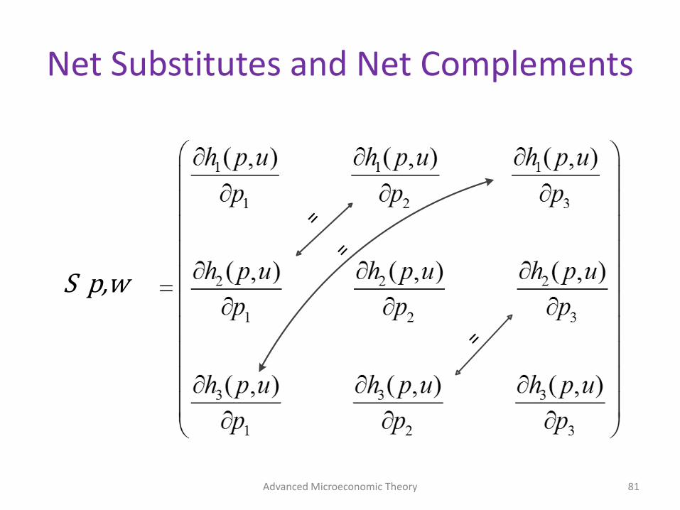
Net Substitutes and Net Complements
Advanced Microeconomic Theory 81
S(p,w)

Net Substitutes and Net Complements
• Proof: – Recall that, from Shephard’s lemma, ℎ𝑘𝑘(𝑝𝑝, 𝑢𝑢) =
𝜕𝜕𝑒𝑒(𝑝𝑝,𝑢𝑢)𝜕𝜕𝑝𝑝𝑘𝑘
. Hence, 𝜕𝜕ℎ𝑘𝑘(𝑝𝑝, 𝑢𝑢)
𝜕𝜕𝑝𝑝𝑗𝑗=
𝜕𝜕2𝑒𝑒(𝑝𝑝, 𝑢𝑢)𝜕𝜕𝑝𝑝𝑘𝑘𝜕𝜕𝑝𝑝𝑗𝑗
– Using Young’s theorem, we obtain𝜕𝜕2𝑒𝑒(𝑝𝑝, 𝑢𝑢)𝜕𝜕𝑝𝑝𝑘𝑘𝜕𝜕𝑝𝑝𝑗𝑗
=𝜕𝜕2𝑒𝑒(𝑝𝑝, 𝑢𝑢)𝜕𝜕𝑝𝑝𝑗𝑗𝜕𝜕𝑝𝑝𝑘𝑘
which implies𝜕𝜕ℎ𝑘𝑘(𝑝𝑝, 𝑢𝑢)
𝜕𝜕𝑝𝑝𝑗𝑗=
𝜕𝜕ℎ𝑗𝑗(𝑝𝑝, 𝑢𝑢)𝜕𝜕𝑝𝑝𝑘𝑘
Advanced Microeconomic Theory 82
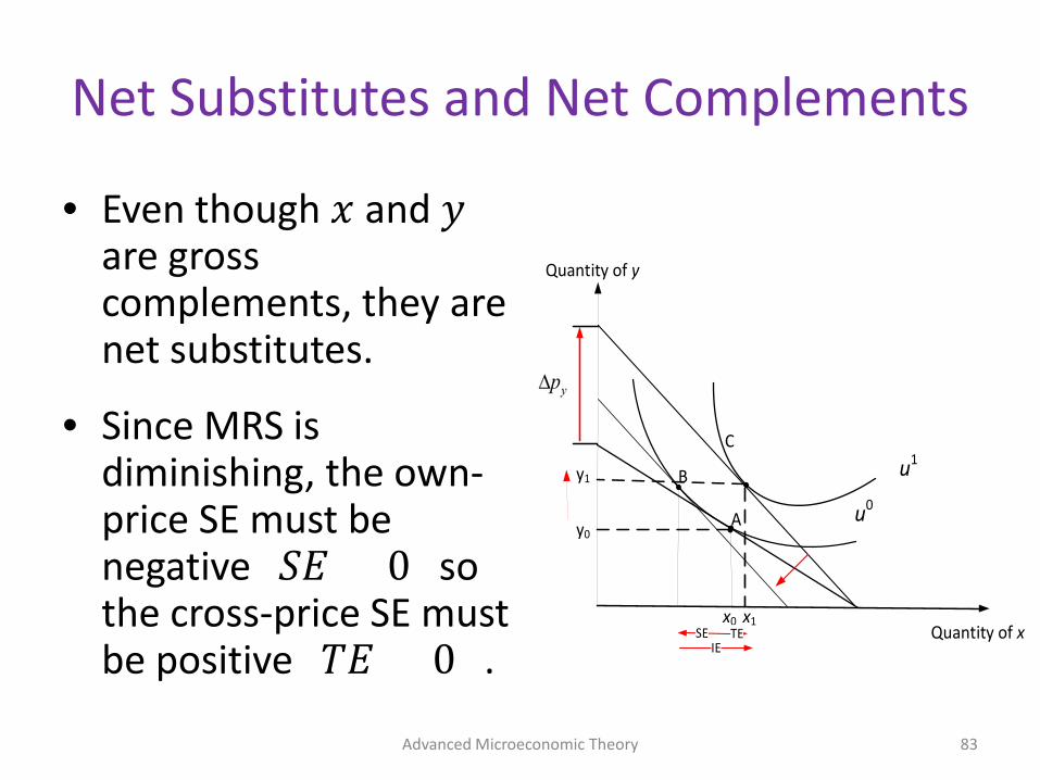
Net Substitutes and Net Complements
• Even though 𝑥𝑥 and 𝑦𝑦are gross complements, they are net substitutes.
• Since MRS is diminishing, the own-price SE must be negative (𝐶𝐶𝐸𝐸 < 0) so the cross-price SE must be positive (𝑇𝑇𝐸𝐸 > 0) .
Advanced Microeconomic Theory 83
Quantity of y
Quantity of x
u1
u0A
B
C
x1x0
y0
y1
IETE
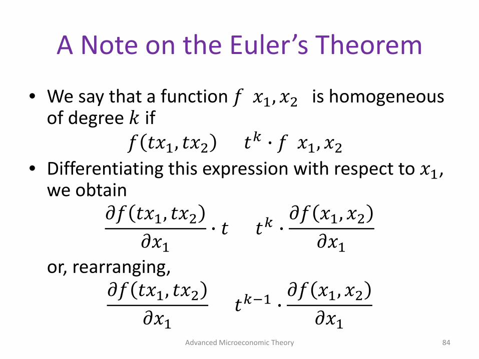
A Note on the Euler’s Theorem
• We say that a function 𝑓𝑓(𝑥𝑥1, 𝑥𝑥2) is homogeneous of degree 𝑘𝑘 if
𝑓𝑓 𝑡𝑡𝑥𝑥1, 𝑡𝑡𝑥𝑥2 = 𝑡𝑡𝑘𝑘 � 𝑓𝑓(𝑥𝑥1, 𝑥𝑥2)• Differentiating this expression with respect to 𝑥𝑥1,
we obtain𝜕𝜕𝑓𝑓 𝑡𝑡𝑥𝑥1, 𝑡𝑡𝑥𝑥2
𝜕𝜕𝑥𝑥1� 𝑡𝑡 = 𝑡𝑡𝑘𝑘 �
𝜕𝜕𝑓𝑓 𝑥𝑥1, 𝑥𝑥2𝜕𝜕𝑥𝑥1
or, rearranging,𝜕𝜕𝑓𝑓 𝑡𝑡𝑥𝑥1, 𝑡𝑡𝑥𝑥2
𝜕𝜕𝑥𝑥1= 𝑡𝑡𝑘𝑘−1 �
𝜕𝜕𝑓𝑓 𝑥𝑥1, 𝑥𝑥2𝜕𝜕𝑥𝑥1
Advanced Microeconomic Theory 84
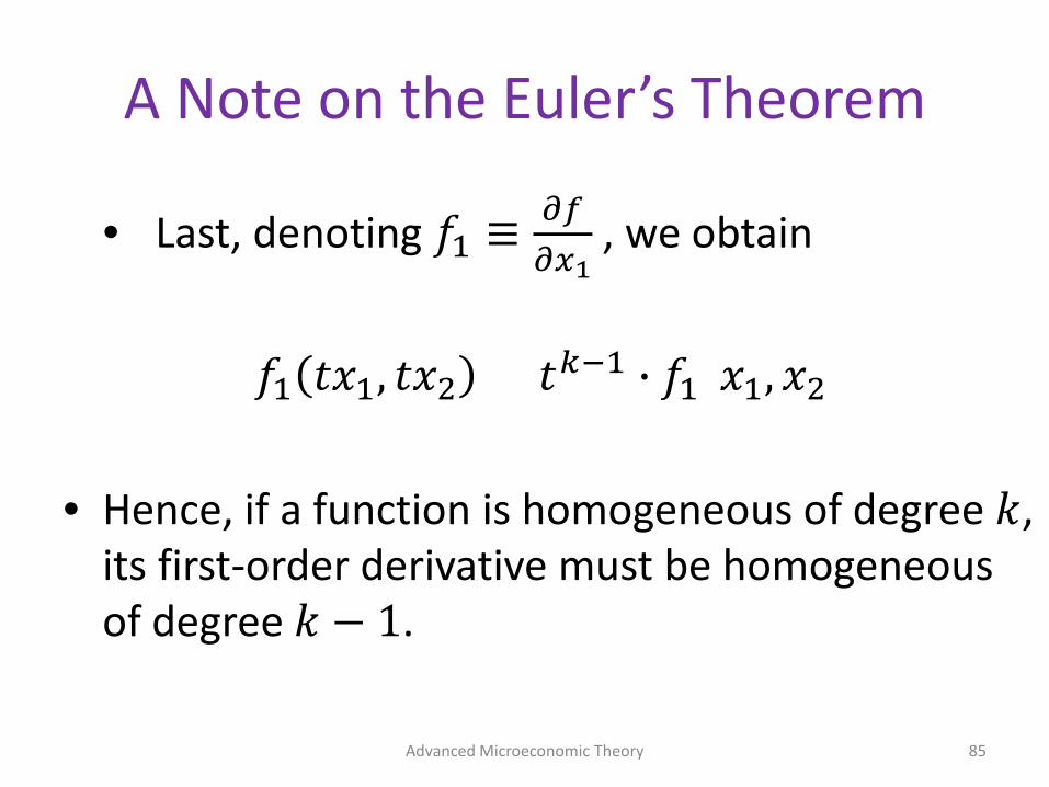
A Note on the Euler’s Theorem
• Last, denoting 𝑓𝑓1 ≡ 𝜕𝜕𝑓𝑓𝜕𝜕𝑥𝑥1
, we obtain
𝑓𝑓1 𝑡𝑡𝑥𝑥1, 𝑡𝑡𝑥𝑥2 = 𝑡𝑡𝑘𝑘−1 � 𝑓𝑓1(𝑥𝑥1, 𝑥𝑥2)
• Hence, if a function is homogeneous of degree 𝑘𝑘, its first-order derivative must be homogeneous of degree 𝑘𝑘 − 1.
Advanced Microeconomic Theory 85
A Note on the Euler’s Theorem
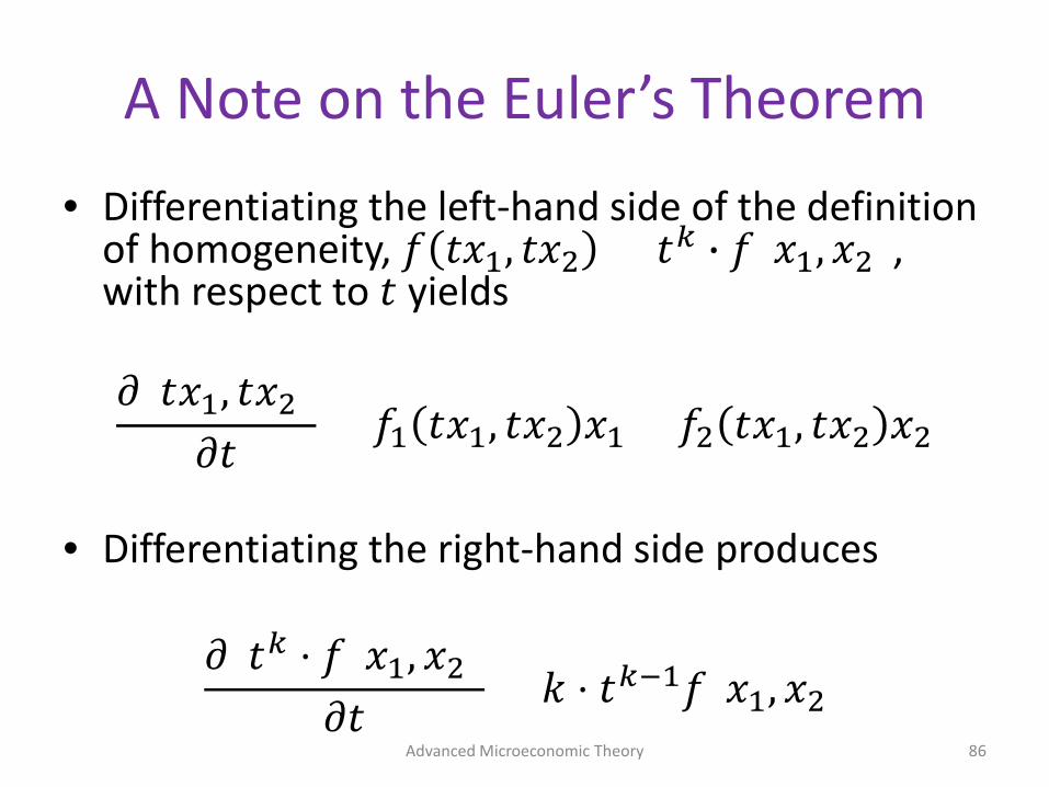
• Differentiating the left-hand side of the definition of homogeneity, 𝑓𝑓 𝑡𝑡𝑥𝑥1, 𝑡𝑡𝑥𝑥2 = 𝑡𝑡𝑘𝑘 � 𝑓𝑓(𝑥𝑥1, 𝑥𝑥2), with respect to 𝑡𝑡 yields
𝜕𝜕(𝑡𝑡𝑥𝑥1, 𝑡𝑡𝑥𝑥2)𝜕𝜕𝑡𝑡
= 𝑓𝑓1 𝑡𝑡𝑥𝑥1, 𝑡𝑡𝑥𝑥2 𝑥𝑥1 + 𝑓𝑓2 𝑡𝑡𝑥𝑥1, 𝑡𝑡𝑥𝑥2 𝑥𝑥2
• Differentiating the right-hand side produces
𝜕𝜕(𝑡𝑡𝑘𝑘 ⋅ 𝑓𝑓(𝑥𝑥1, 𝑥𝑥2)𝜕𝜕𝑡𝑡
= 𝑘𝑘 ⋅ 𝑡𝑡𝑘𝑘−1𝑓𝑓(𝑥𝑥1, 𝑥𝑥2)Advanced Microeconomic Theory 86
A Note on the Euler’s Theorem
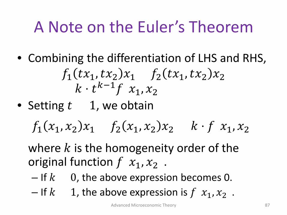
• Combining the differentiation of LHS and RHS, 𝑓𝑓1 𝑡𝑡𝑥𝑥1, 𝑡𝑡𝑥𝑥2 𝑥𝑥1 + 𝑓𝑓2 𝑡𝑡𝑥𝑥1, 𝑡𝑡𝑥𝑥2 𝑥𝑥2= 𝑘𝑘 ⋅ 𝑡𝑡𝑘𝑘−1𝑓𝑓(𝑥𝑥1, 𝑥𝑥2)
• Setting 𝑡𝑡 = 1, we obtain
𝑓𝑓1 𝑥𝑥1, 𝑥𝑥2 𝑥𝑥1 + 𝑓𝑓2 𝑥𝑥1, 𝑥𝑥2 𝑥𝑥2 = 𝑘𝑘 ⋅ 𝑓𝑓(𝑥𝑥1, 𝑥𝑥2)
where 𝑘𝑘 is the homogeneity order of the original function 𝑓𝑓(𝑥𝑥1, 𝑥𝑥2).– If 𝑘𝑘 = 0, the above expression becomes 0.– If 𝑘𝑘 = 1, the above expression is 𝑓𝑓(𝑥𝑥1, 𝑥𝑥2).
Advanced Microeconomic Theory 87
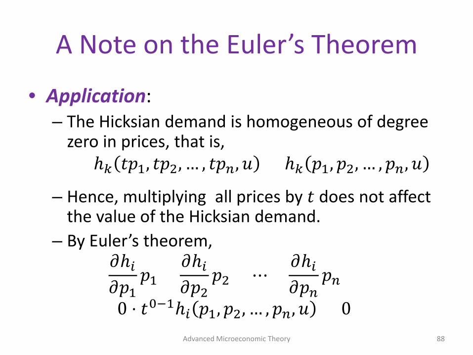
A Note on the Euler’s Theorem
• Application:– The Hicksian demand is homogeneous of degree
zero in prices, that is,ℎ𝑘𝑘 𝑡𝑡𝑝𝑝1, 𝑡𝑡𝑝𝑝2, … , 𝑡𝑡𝑝𝑝𝑛𝑛, 𝑢𝑢 = ℎ𝑘𝑘 𝑝𝑝1, 𝑝𝑝2, … , 𝑝𝑝𝑛𝑛, 𝑢𝑢
– Hence, multiplying all prices by 𝑡𝑡 does not affect the value of the Hicksian demand.
– By Euler’s theorem,𝜕𝜕ℎ𝑖𝑖
𝜕𝜕𝑝𝑝1𝑝𝑝1 +
𝜕𝜕ℎ𝑖𝑖
𝜕𝜕𝑝𝑝2𝑝𝑝2 + ⋯ +
𝜕𝜕ℎ𝑖𝑖
𝜕𝜕𝑝𝑝𝑛𝑛𝑝𝑝𝑛𝑛
= 0 ⋅ 𝑡𝑡0−1ℎ𝑖𝑖 𝑝𝑝1, 𝑝𝑝2, … , 𝑝𝑝𝑛𝑛, 𝑢𝑢 = 0Advanced Microeconomic Theory 88

Substitutability with Many Goods• Question: Is net substitutability or complementarity
more prevalent in real life?• To answer this question, we can start with the
compensated demand functionℎ𝑘𝑘 𝑝𝑝1, 𝑝𝑝2, … , 𝑝𝑝𝑛𝑛, 𝑢𝑢
• Applying Euler’s theorem yields𝜕𝜕ℎ𝑘𝑘
𝜕𝜕𝑝𝑝1𝑝𝑝1 +
𝜕𝜕ℎ𝑘𝑘
𝜕𝜕𝑝𝑝2𝑝𝑝2 + ⋯ +
𝜕𝜕ℎ𝑘𝑘
𝜕𝜕𝑝𝑝𝑛𝑛𝑝𝑝𝑛𝑛 = 0
• Dividing both sides by ℎ𝑘𝑘, we can alternatively express the above result using compensated elasticities
𝜀𝜀𝑖𝑖1 + 𝜀𝜀𝑖𝑖2 + ⋯ + 𝜀𝜀𝑖𝑖𝑛𝑛 ≡ 0Advanced Microeconomic Theory 89
Substitutability with Many Goods
• Since the negative sign of the SE implies that 𝜀𝜀𝑖𝑖𝑖𝑖 ≤ 0, then the sum of Hicksian cross-price
elasticities for all other 𝑗𝑗 ≠ 𝑖𝑖 goods should satisfy
�𝑗𝑗≠𝑖𝑖
𝜀𝜀𝑖𝑖𝑗𝑗 ≥ 0
• Hence, “most” goods must be substitutes.• This is referred to as Hick’s second law of
demand.Advanced Microeconomic Theory 90

Aggregate Demand
Advanced Microeconomic Theory 91
Aggregate Demand
• We now move from individual demand, 𝑥𝑥𝑖𝑖(𝑝𝑝, 𝑤𝑤𝑖𝑖), to aggregate demand,
�𝑖𝑖=1
𝐼𝐼
𝑥𝑥𝑖𝑖(𝑝𝑝, 𝑤𝑤𝑖𝑖)
which denotes the total demand of a group of 𝐼𝐼 consumers.
• Individual 𝑖𝑖’s demand 𝑥𝑥𝑖𝑖(𝑝𝑝, 𝑤𝑤𝑖𝑖) still represents a vector of 𝐷𝐷 components, describing his demand for 𝐷𝐷 different goods.
Advanced Microeconomic Theory 92
Aggregate Demand
• We know individual demand depends on prices and individual’s wealth.– When can we express aggregate demand as a function
of prices and aggregate wealth?– In other words, when can we guarantee that
aggregate demand defined as 𝑥𝑥 𝑝𝑝, 𝑤𝑤1, 𝑤𝑤2, … , 𝑤𝑤𝐼𝐼 = ∑𝑖𝑖=1
𝐼𝐼 𝑥𝑥𝑖𝑖(𝑝𝑝, 𝑤𝑤𝑖𝑖)satisfies
�𝑖𝑖=1
𝐼𝐼
𝑥𝑥𝑖𝑖(𝑝𝑝, 𝑤𝑤𝑖𝑖) = 𝑥𝑥 𝑝𝑝, �𝑖𝑖=1
𝐼𝐼
𝑤𝑤𝑖𝑖
Advanced Microeconomic Theory 93
Aggregate Demand
• This is satisfied if, for any two distributions of wealth, (𝑤𝑤1, 𝑤𝑤2, … , 𝑤𝑤𝐼𝐼) and (𝑤𝑤1
′ , 𝑤𝑤2′ , … , 𝑤𝑤𝐼𝐼
′) such that ∑𝑖𝑖=1
𝐼𝐼 𝑤𝑤𝑖𝑖 = ∑𝑖𝑖=1𝐼𝐼 𝑤𝑤𝑖𝑖
′, we have
�𝑖𝑖=1
𝐼𝐼
𝑥𝑥𝑖𝑖(𝑝𝑝, 𝑤𝑤𝑖𝑖) = �𝑖𝑖=1
𝐼𝐼
𝑥𝑥𝑖𝑖(𝑝𝑝, 𝑤𝑤𝑖𝑖′)
• For such condition to be satisfied, let’s start with an initial distribution (𝑤𝑤1, 𝑤𝑤2, … , 𝑤𝑤𝐼𝐼) and apply a differential change in wealth (𝑑𝑑𝑤𝑤1, 𝑑𝑑𝑤𝑤2, … , 𝑑𝑑𝑤𝑤𝐼𝐼)such that the aggregate wealth is unchanged, ∑𝑖𝑖=1
𝐼𝐼 𝑑𝑑𝑤𝑤𝑖𝑖 = 0.Advanced Microeconomic Theory 94
Aggregate Demand
• If aggregate demand is just a function of aggregate wealth, then we must have that
∑𝑖𝑖=1𝐼𝐼 𝜕𝜕𝑥𝑥𝑖𝑖(𝑝𝑝,𝑤𝑤𝑖𝑖)
𝜕𝜕𝑤𝑤𝑖𝑖𝑑𝑑𝑤𝑤𝑖𝑖 = 0 for every good 𝑘𝑘
In words, the wealth effects of different individuals are compensated in the aggregate. That is, in the case of two individuals 𝑖𝑖 and 𝑗𝑗,
𝜕𝜕𝑥𝑥𝑘𝑘𝑖𝑖(𝑝𝑝, 𝑤𝑤𝑖𝑖)𝜕𝜕𝑤𝑤𝑖𝑖
=𝜕𝜕𝑥𝑥𝑘𝑘𝑗𝑗(𝑝𝑝, 𝑤𝑤𝑗𝑗)
𝜕𝜕𝑤𝑤𝑗𝑗
for every good 𝑘𝑘.Advanced Microeconomic Theory 95
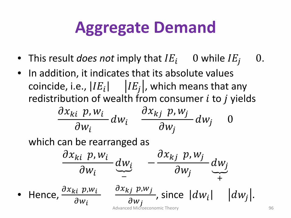
Aggregate Demand
• This result does not imply that 𝐼𝐼𝐸𝐸𝑖𝑖 > 0 while 𝐼𝐼𝐸𝐸𝑗𝑗 < 0.• In addition, it indicates that its absolute values
coincide, i.e., 𝐼𝐼𝐸𝐸𝑖𝑖 = 𝐼𝐼𝐸𝐸𝑗𝑗 , which means that any redistribution of wealth from consumer 𝑖𝑖 to 𝑗𝑗 yields
𝜕𝜕𝑥𝑥𝑘𝑘𝑖𝑖(𝑝𝑝, 𝑤𝑤𝑖𝑖)𝜕𝜕𝑤𝑤𝑖𝑖
𝑑𝑑𝑤𝑤𝑖𝑖 +𝜕𝜕𝑥𝑥𝑘𝑘𝑗𝑗(𝑝𝑝, 𝑤𝑤𝑗𝑗)
𝜕𝜕𝑤𝑤𝑗𝑗𝑑𝑑𝑤𝑤𝑗𝑗 = 0
which can be rearranged as𝜕𝜕𝑥𝑥𝑘𝑘𝑖𝑖(𝑝𝑝, 𝑤𝑤𝑖𝑖)
𝜕𝜕𝑤𝑤𝑖𝑖�𝑑𝑑𝑤𝑤𝑖𝑖
−= −
𝜕𝜕𝑥𝑥𝑘𝑘𝑗𝑗(𝑝𝑝, 𝑤𝑤𝑗𝑗)𝜕𝜕𝑤𝑤𝑗𝑗
�𝑑𝑑𝑤𝑤𝑗𝑗+
• Hence, 𝜕𝜕𝑥𝑥𝑘𝑘𝑖𝑖(𝑝𝑝,𝑤𝑤𝑖𝑖)𝜕𝜕𝑤𝑤𝑖𝑖
= 𝜕𝜕𝑥𝑥𝑘𝑘𝑗𝑗(𝑝𝑝,𝑤𝑤𝑗𝑗)𝜕𝜕𝑤𝑤𝑗𝑗
, since 𝑑𝑑𝑤𝑤𝑖𝑖 = 𝑑𝑑𝑤𝑤𝑗𝑗 .Advanced Microeconomic Theory 96
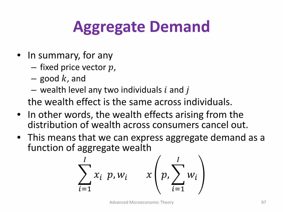
Aggregate Demand• In summary, for any
– fixed price vector 𝑝𝑝,– good 𝑘𝑘, and– wealth level any two individuals 𝑖𝑖 and 𝑗𝑗
the wealth effect is the same across individuals.• In other words, the wealth effects arising from the
distribution of wealth across consumers cancel out.• This means that we can express aggregate demand as a
function of aggregate wealth
�𝑖𝑖=1
𝐼𝐼
𝑥𝑥𝑖𝑖(𝑝𝑝, 𝑤𝑤𝑖𝑖) = 𝑥𝑥 𝑝𝑝, �𝑖𝑖=1
𝐼𝐼
𝑤𝑤𝑖𝑖
Advanced Microeconomic Theory 97

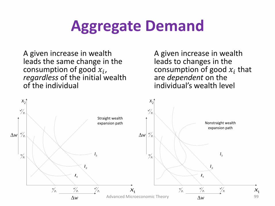
Aggregate Demand
• Graphically, this condition entails that all consumers exhibit parallel, straight wealth expansion paths. – Straight: wealth effects do not depend on the
individuals’ wealth level.– Parallel: individuals’ wealth effects must coincide
across individuals. Recall that wealth expansion paths just represent how
an individual demand changes as he becomes richer.
Advanced Microeconomic Theory 98
Aggregate Demand
Advanced Microeconomic Theory 99
Straight wealth expansion path
1l
2l
3l
1x
2x
1
wp 1
wp′
1
wp
′′
1
wp
′′
1
wp′
1
wp
w∆
w∆
Nonstraight wealth expansion path
1l
2l
3l
1x
2x
1
wp 1
wp′
1
wp
′′
1
wp
′′
1
wp′
1
wp
w∆
w∆
A given increase in wealth leads to changes in the consumption of good 𝑥𝑥𝑖𝑖 that are dependent on the individual’s wealth level
A given increase in wealth leads the same change in the consumption of good 𝑥𝑥𝑖𝑖, regardless of the initial wealth of the individual

Aggregate Demand
• Individuals’ wealth effects coincide.
• The wealth expansion path for consumers 1 and 2 are parallel to each other– both individuals’
demands change similarly as they become richer.
Advanced Microeconomic Theory 100
2x
1x
1,p wB
2,p wB
Wealth expansion path for consumer 1
Wealth expansion path for consumer 2

Aggregate Demand
• Preference relations that yield straight wealth expansion paths:– Homothetic preferences– Quasilinear preferences
• Can we embody all these cases as special cases of a particular type of preferences?– Yes. We next present such cases.
Advanced Microeconomic Theory 101
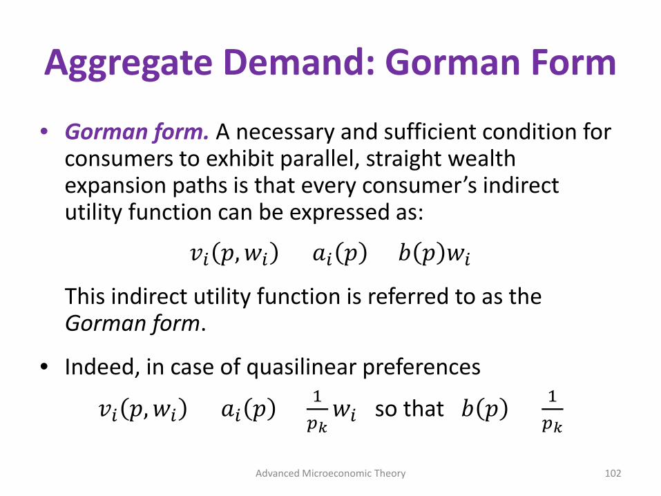
Aggregate Demand: Gorman Form
• Gorman form. A necessary and sufficient condition for consumers to exhibit parallel, straight wealth expansion paths is that every consumer’s indirect utility function can be expressed as:
𝑣𝑣𝑖𝑖 𝑝𝑝, 𝑤𝑤𝑖𝑖 = 𝑎𝑎𝑖𝑖 𝑝𝑝 + 𝑏𝑏 𝑝𝑝 𝑤𝑤𝑖𝑖
This indirect utility function is referred to as the Gorman form.
• Indeed, in case of quasilinear preferences
𝑣𝑣𝑖𝑖 𝑝𝑝, 𝑤𝑤𝑖𝑖 = 𝑎𝑎𝑖𝑖 𝑝𝑝 + 1𝑝𝑝𝑘𝑘
𝑤𝑤𝑖𝑖 so that 𝑏𝑏 𝑝𝑝 = 1𝑝𝑝𝑘𝑘
Advanced Microeconomic Theory 102
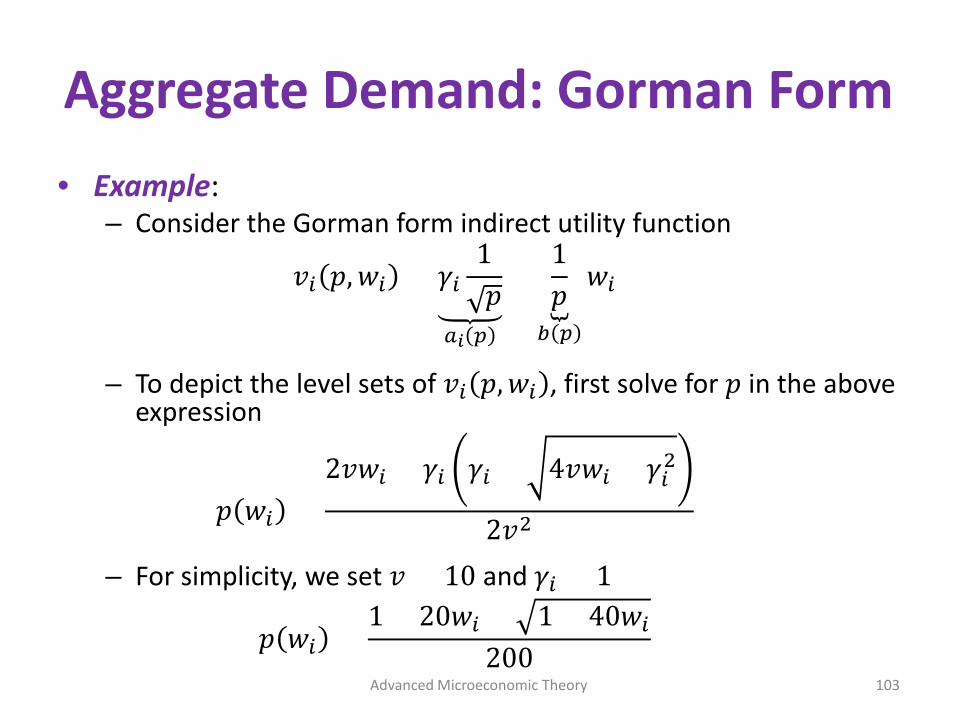
Aggregate Demand: Gorman Form• Example:
– Consider the Gorman form indirect utility function
𝑣𝑣𝑖𝑖 𝑝𝑝, 𝑤𝑤𝑖𝑖 = 𝛾𝛾𝑖𝑖1𝑝𝑝
𝐽𝐽𝑖𝑖 𝑝𝑝
+⏟1𝑝𝑝
𝑏𝑏 𝑝𝑝
𝑤𝑤𝑖𝑖
– To depict the level sets of 𝑣𝑣𝑖𝑖 𝑝𝑝, 𝑤𝑤𝑖𝑖 , first solve for 𝑝𝑝 in the above expression
𝑝𝑝 𝑤𝑤𝑖𝑖 =2𝑣𝑣𝑤𝑤𝑖𝑖 + 𝛾𝛾𝑖𝑖 𝛾𝛾𝑖𝑖 + 4𝑣𝑣𝑤𝑤𝑖𝑖 + 𝛾𝛾𝑖𝑖
2
2𝑣𝑣2
– For simplicity, we set 𝑣𝑣 = 10 and 𝛾𝛾𝑖𝑖 = 1
𝑝𝑝 𝑤𝑤𝑖𝑖 =1 + 20𝑤𝑤𝑖𝑖 + 1 + 40𝑤𝑤𝑖𝑖
200Advanced Microeconomic Theory 103
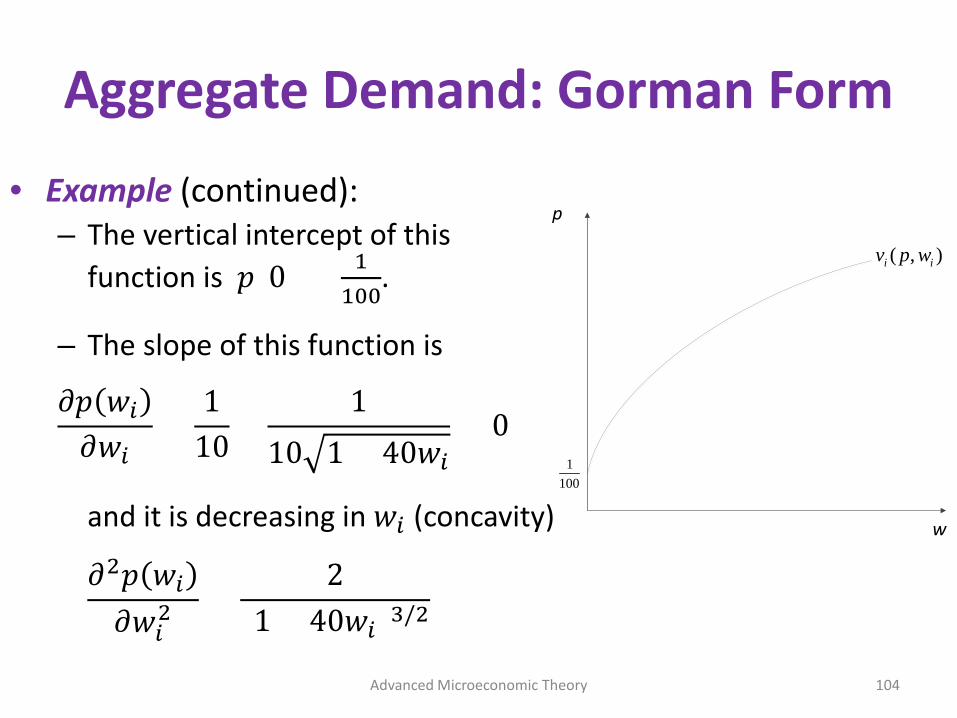
Aggregate Demand: Gorman Form
• Example (continued):– The vertical intercept of this
function is 𝑝𝑝(0) = 1100
.
– The slope of this function is
𝜕𝜕𝑝𝑝 𝑤𝑤𝑖𝑖
𝜕𝜕𝑤𝑤𝑖𝑖=
110
+1
10 1 + 40𝑤𝑤𝑖𝑖> 0
and it is decreasing in 𝑤𝑤𝑖𝑖 (concavity)
𝜕𝜕2𝑝𝑝 𝑤𝑤𝑖𝑖
𝜕𝜕𝑤𝑤𝑖𝑖2 =
2(1 + 40𝑤𝑤𝑖𝑖)3/2
Advanced Microeconomic Theory 104
p
w
1100
( , )i iv p w
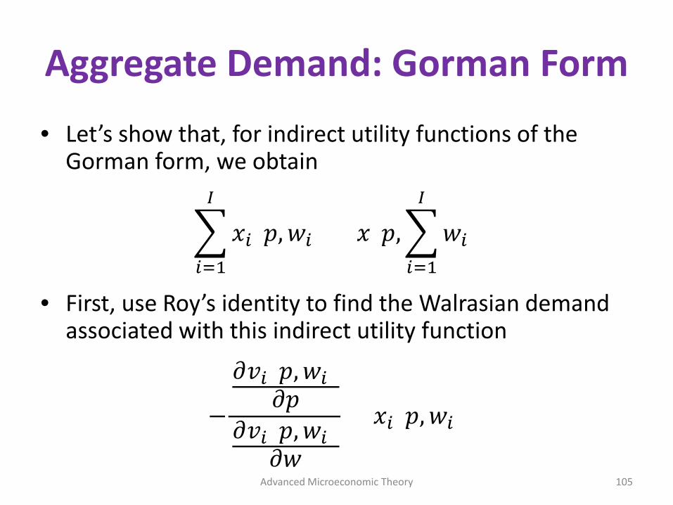
Aggregate Demand: Gorman Form
• Let’s show that, for indirect utility functions of the Gorman form, we obtain
�𝑖𝑖=1
𝐼𝐼
𝑥𝑥𝑖𝑖(𝑝𝑝, 𝑤𝑤𝑖𝑖) = 𝑥𝑥(𝑝𝑝, �𝑖𝑖=1
𝐼𝐼
𝑤𝑤𝑖𝑖)
• First, use Roy’s identity to find the Walrasian demand associated with this indirect utility function
−
𝜕𝜕𝑣𝑣𝑖𝑖(𝑝𝑝, 𝑤𝑤𝑖𝑖)𝜕𝜕𝑝𝑝
𝜕𝜕𝑣𝑣𝑖𝑖(𝑝𝑝, 𝑤𝑤𝑖𝑖)𝜕𝜕𝑤𝑤
= 𝑥𝑥𝑖𝑖(𝑝𝑝, 𝑤𝑤𝑖𝑖)
Advanced Microeconomic Theory 105
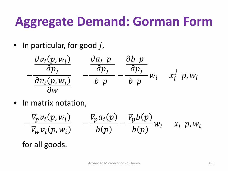
Aggregate Demand: Gorman Form
• In particular, for good 𝑗𝑗,
−
𝜕𝜕𝑣𝑣𝑖𝑖 𝑝𝑝, 𝑤𝑤𝑖𝑖𝜕𝜕𝑝𝑝𝑗𝑗
𝜕𝜕𝑣𝑣𝑖𝑖 𝑝𝑝, 𝑤𝑤𝑖𝑖𝜕𝜕𝑤𝑤
= −
𝜕𝜕𝑎𝑎𝑖𝑖(𝑝𝑝)𝜕𝜕𝑝𝑝𝑗𝑗
𝑏𝑏(𝑝𝑝)−
𝜕𝜕𝑏𝑏(𝑝𝑝)𝜕𝜕𝑝𝑝𝑗𝑗
𝑏𝑏(𝑝𝑝)𝑤𝑤𝑖𝑖 = 𝑥𝑥𝑖𝑖
𝑗𝑗(𝑝𝑝, 𝑤𝑤𝑖𝑖)
• In matrix notation,
−𝛻𝛻𝑝𝑝𝑣𝑣𝑖𝑖 𝑝𝑝, 𝑤𝑤𝑖𝑖
𝛻𝛻𝑤𝑤𝑣𝑣𝑖𝑖 𝑝𝑝, 𝑤𝑤𝑖𝑖= −
𝛻𝛻𝑝𝑝𝑎𝑎𝑖𝑖 𝑝𝑝𝑏𝑏 𝑝𝑝
−𝛻𝛻𝑝𝑝𝑏𝑏 𝑝𝑝
𝑏𝑏 𝑝𝑝𝑤𝑤𝑖𝑖 = 𝑥𝑥𝑖𝑖(𝑝𝑝, 𝑤𝑤𝑖𝑖)
for all goods.
Advanced Microeconomic Theory 106
Aggregate Demand: Gorman Form
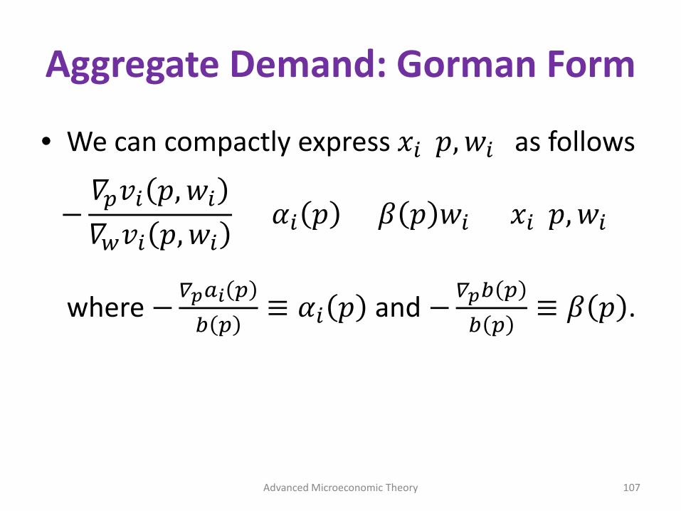
• We can compactly express 𝑥𝑥𝑖𝑖(𝑝𝑝, 𝑤𝑤𝑖𝑖) as follows
−𝛻𝛻𝑝𝑝𝑣𝑣𝑖𝑖 𝑝𝑝, 𝑤𝑤𝑖𝑖
𝛻𝛻𝑤𝑤𝑣𝑣𝑖𝑖 𝑝𝑝, 𝑤𝑤𝑖𝑖= 𝛼𝛼𝑖𝑖 𝑝𝑝 + 𝛽𝛽 𝑝𝑝 𝑤𝑤𝑖𝑖 = 𝑥𝑥𝑖𝑖(𝑝𝑝, 𝑤𝑤𝑖𝑖)
where − 𝛻𝛻𝑝𝑝𝐽𝐽𝑖𝑖 𝑝𝑝𝑏𝑏 𝑝𝑝
≡ 𝛼𝛼𝑖𝑖 𝑝𝑝 and − 𝛻𝛻𝑝𝑝𝑏𝑏 𝑝𝑝𝑏𝑏 𝑝𝑝
≡ 𝛽𝛽 𝑝𝑝 .
Advanced Microeconomic Theory 107
Aggregate Demand: Gorman Form
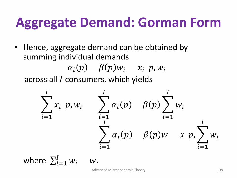
• Hence, aggregate demand can be obtained by summing individual demands
𝛼𝛼𝑖𝑖 𝑝𝑝 + 𝛽𝛽 𝑝𝑝 𝑤𝑤𝑖𝑖 = 𝑥𝑥𝑖𝑖(𝑝𝑝, 𝑤𝑤𝑖𝑖)across all 𝐼𝐼 consumers, which yields
�𝑖𝑖=1
𝐼𝐼
𝑥𝑥𝑖𝑖(𝑝𝑝, 𝑤𝑤𝑖𝑖) = �𝑖𝑖=1
𝐼𝐼
𝛼𝛼𝑖𝑖 𝑝𝑝 + 𝛽𝛽 𝑝𝑝 �𝑖𝑖=1
𝐼𝐼
𝑤𝑤𝑖𝑖
= �𝑖𝑖=1
𝐼𝐼
𝛼𝛼𝑖𝑖 𝑝𝑝 + 𝛽𝛽 𝑝𝑝 𝑤𝑤 = 𝑥𝑥(𝑝𝑝, �𝑖𝑖=1
𝐼𝐼
𝑤𝑤𝑖𝑖)
where ∑𝑖𝑖=1𝐼𝐼 𝑤𝑤𝑖𝑖 = 𝑤𝑤.
Advanced Microeconomic Theory 108