Advanced Mesh-Enabled Monte Carlo Capability for Multi-Physics

Reactor Analysis

Fuel Cycle R&D Dr. Paul Wilson

University of Wisconsin, Madison

In collaboration with: Alamos National Laboratory

Oak Ridge National Laboratory

Rob Versluis, Federal POC Tim Tautges, Technical POC

Project No. 09-786

Advanced Mesh-Enabled Monte Carlo Capability for Multi-Physics Reactor Analysis

Final Report: 10/2009 – 09/2012

PI: Paul Wilson, UW-Madison

Co-PIs: Tom Evans, ORNL

Tim Tautges, ANL

Overview Continuous energy Monte Carlo methods are generally considered to be the most accurate computational tool for simulating radiation transport in complex geometries, particularly neutron transport in reactor geometries. Nevertheless, there are several limitations to Monte Carlo methods for use in reactor analysis. Most prominently, there is a trade-off between the fidelity of the results in phase space, the statistical accuracy, and the amount of computer time required for simulation. Consequently, to achieve an acceptable level of statistical convergence in high-fidelity results required for modern coupled multi-physics analysis, the required computer time makes Monte Carlo methods prohibitive for design iterations and detailed whole-core analysis. More subtly, the statistical uncertainty is typically not uniform throughout the domain and the quality of the simulation is limited by the regions with the largest statistical uncertainty. In addition, the formulation of the neutron scattering laws in continuous energy Monte Carlo methods makes it difficult to calculate adjoint neutron fluxes that are so important to properly determine important reactivity parameters. Finally, most Monte Carlo codes available for reactor analysis have relied on orthogonal hexahedral grids for tallies that do not conform to the geometric boundaries and are thus generally not well-suited to coupling with the unstructured meshes that are used in other physics simulations.

The outcome of this work is the efficient accumulation of high precision fluxes (everywhere) throughout a reactor geometry on a non-orthogonal grid of cells to support multi-physics coupling, to more accurately calculate parameters such as reactivity coefficients, and perhaps to generate multi-group cross sections. This work is based upon previous developments by the lead institution (UW-Madison) to incorporate advanced geometry and mesh capability in the modular Direct Accelerated Geometry Monte Carlo (DAGMC) toolkit using the Mesh Oriented Database (MOAB) technology developed under support of the DOE SciDAC program, and maintained by partner Argonne National Laboratory. Coupling this capability with production scale Monte Carlo radiation transport codes under ongoing development at partner Oak Ridge National Laboratory, can provide advanced and extensible test-beds for these developments.

Task 1: Implement Track-Length Tally in Unstructured Mesh The Direct Accelerated Geometry for Monte Carlo (DAGMC) library [1] has been extended to include support of track length tallies on unstructured meshes. There is a growing demand for high-fidelity mesh tallies in Monte Carlo radiation transport, driven in part by a combination of the ability to model complex CAD-based geometries and the desire to couple these results to simulations of other physics. In most Monte Carlo tools, including MCNP5 [2] used as the target code in this work, high fidelity, large domain tallies have been performed on orthogonal structured grids that overlay the geometry unaware of material boundaries. This work provides the ability to perform tallies on any tetrahedral mesh, particularly mesh that conforms to material boundaries.

To examine the challenge of the current technology for high-fidelity mesh tallies, consider the straightforward task of determining the nuclear heating in an array of cylinders (e.g. a nuclear fuel assembly or a fusion shield block [3]). Traditional mesh tallies provided two options for the single volume-averaged result tallied in voxels that included more than a single material: a result based on using the correct cross-sections for each track in the voxel or a result based on a using a single cross-section for all tracks in the voxel. The former provides a correct result for the voxel, but can possibly be a poor approximation for any of the materials in the voxel. The latter is not correct for the voxel, but may provide a better approximation for the material corresponding to the cross-section used for tallying. Therefore, one approach is to perform multiple geometrically identical mesh tallies over the same domain and use a different cross-section for each – one mesh tally per material. For mesh with many voxels, this can begin to challenge hardware memory limitations. Even once such approximations are invoked, it is often necessary to interpolate/integrate these results onto an unstructured mesh for use in other physics simulations.

Another recent innovation has introduced an unstructured mesh to MCNP for both geometry definition and tallies [4], but requires that both tracking and tallying occur on the mesh. The present work adds an unstructured mesh to problems with geometries defined in other ways, including the native geometry description and the DAGMC CAD-based description. While unstructured mesh is not generally guaranteed to be conformal to material boundaries, this effort is focused on mesh that is generated from the same CAD-based geometry description that is used for transport. These meshes will be conformal to the material interfaces and may be optimized for other types of physics simulations, such as CFD and heat transfer.

Method overview and implementation

The tracking phase of the Monte Carlo simulation is undisturbed by this extension. Particle histories are followed by using the standard sampling of flight distance and comparing that to the distance to material boundaries found by ray-firing techniques. Thus an increment of particle history is found in which both end points represent either collision events or surface crossing events. This linear track is then sent to the mesh tally routine to rigorously allocate the track across the tetrahedra in the mesh. The allocation of track length across a mesh in this fashion

will be faster than tracking across that mesh, since the variety of geometry and physics tests that are done at geometric boundaries are avoided at each mesh element boundary.

It is necessary for this method to efficiently determine when a particle is born inside a mesh or enters a mesh from a region that is not in the mesh. By implementing this solution using the DAGMC toolkit, we are able to use existing point location and ray-firing tests on the skin of the mesh, as well as search algorithms within the underlying Mesh Oriented database (MOAB) [5] to determine which mesh element contains a track end point.

From the user’s perspective, these tallies are implemented as an extension of the FMESH card, offering an addition type for GEOM=keyword and using the FC tally comment card to embed additional parameters for the mesh. The unstructured mesh is treated as an overlay to the geometry, much as the traditional structured tally grids, so the geometry description is unchanged. It is up to the user to provide a mesh that resolves the boundaries of interest.

Testing A number of simple problems were devised for testing the results. All problems have a source of mono-directional, mono-energetic (1 MeV) neutrons, directed down the length of long rectangular block. Reflecting boundaries in the directions transverse to the beam are used in all problems, except problem 2 with vacuum boundaries. In all cases, the neutrons enter a region of water ( =1g/cm3). Table I summarizes the other features of the 6 different cases. In problems 3-6, an interface was introduced. This combination of problems tests the effect of different interface orientations, first as purely geometric interfaces and then as material interfaces. Tests 1-3 and test 5 are designed as verification tests and the results in the unstructured mesh are consistent with the results in the traditional MCNP5 structured mesh. Tests 4 and 6 are designed to highlight the differences between the unstructured mesh tallies and the traditional structured mesh tallies.

Since the new tallies and the traditional tallies can co-exist in a single geometry, tally results were computed for both a traditional Cartesian grid and a tetrahedral grid in the same simulation. Some sample results are shown in Figures 1 and 2, but a robust method for numerical comparison is

Table I. Summary of Test Problem Features

Test #

Boundary Conditions

Interface Material

Interface Orientation

1 Reflecting N/A N/A

2 Vacuum N/A N/A

3 Reflecting Water Perpendicular

4 Reflecting Cd (=7 g/cm3)

Perpendicular

5 Reflecting Water Oblique

6 Reflecting Cd (=7 g/cm3)

Oblique

still under investigation.

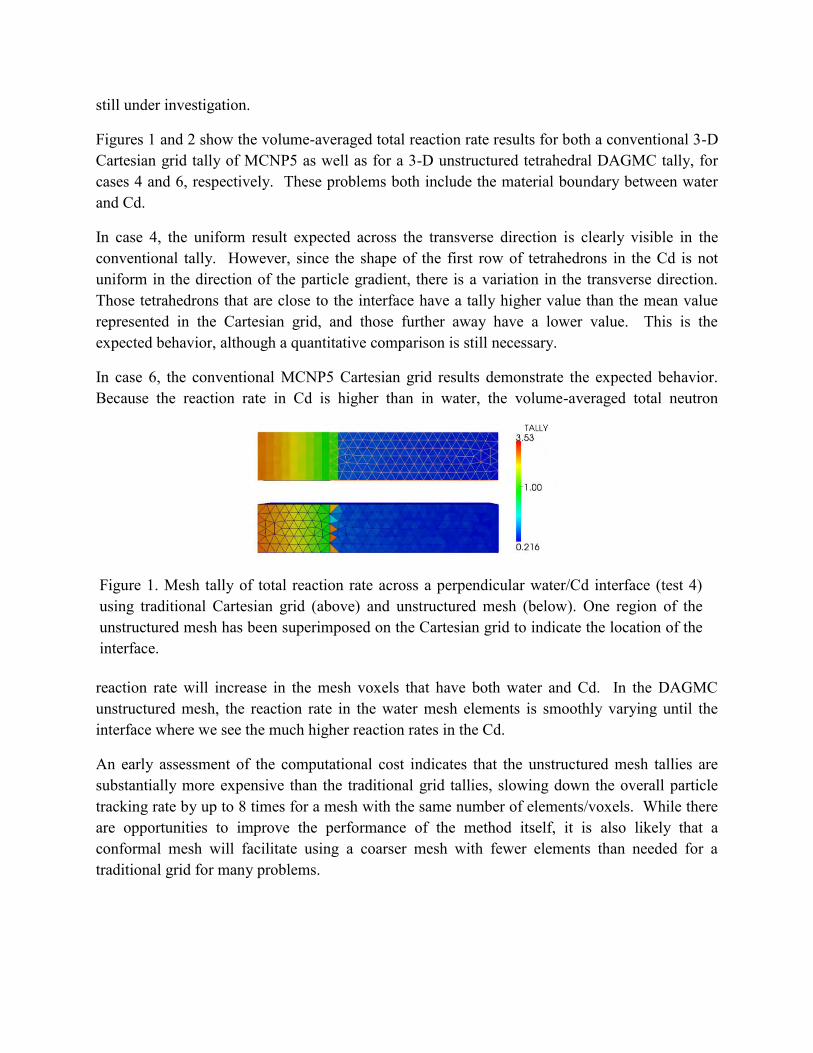
Figures 1 and 2 show the volume-averaged total reaction rate results for both a conventional 3-D Cartesian grid tally of MCNP5 as well as for a 3-D unstructured tetrahedral DAGMC tally, for cases 4 and 6, respectively. These problems both include the material boundary between water and Cd.

In case 4, the uniform result expected across the transverse direction is clearly visible in the conventional tally. However, since the shape of the first row of tetrahedrons in the Cd is not uniform in the direction of the particle gradient, there is a variation in the transverse direction. Those tetrahedrons that are close to the interface have a tally higher value than the mean value represented in the Cartesian grid, and those further away have a lower value. This is the expected behavior, although a quantitative comparison is still necessary.

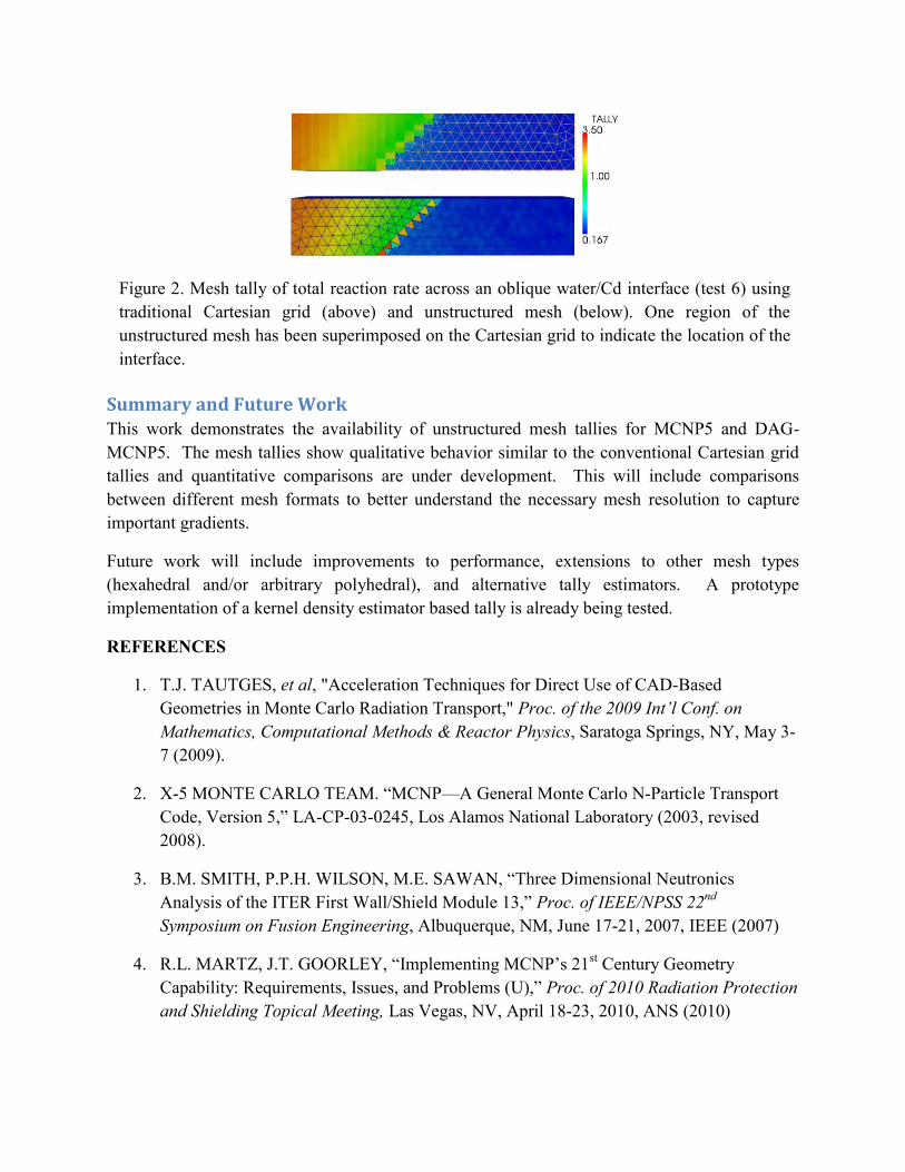
In case 6, the conventional MCNP5 Cartesian grid results demonstrate the expected behavior. Because the reaction rate in Cd is higher than in water, the volume-averaged total neutron

reaction rate will increase in the mesh voxels that have both water and Cd. In the DAGMC unstructured mesh, the reaction rate in the water mesh elements is smoothly varying until the interface where we see the much higher reaction rates in the Cd.

An early assessment of the computational cost indicates that the unstructured mesh tallies are substantially more expensive than the traditional grid tallies, slowing down the overall particle tracking rate by up to 8 times for a mesh with the same number of elements/voxels. While there are opportunities to improve the performance of the method itself, it is also likely that a conformal mesh will facilitate using a coarser mesh with fewer elements than needed for a traditional grid for many problems.

Figure 1. Mesh tally of total reaction rate across a perpendicular water/Cd interface (test 4) using traditional Cartesian grid (above) and unstructured mesh (below). One region of the unstructured mesh has been superimposed on the Cartesian grid to indicate the location of the interface.

Summary and Future Work This work demonstrates the availability of unstructured mesh tallies for MCNP5 and DAG-MCNP5. The mesh tallies show qualitative behavior similar to the conventional Cartesian grid tallies and quantitative comparisons are under development. This will include comparisons between different mesh formats to better understand the necessary mesh resolution to capture important gradients.

Future work will include improvements to performance, extensions to other mesh types (hexahedral and/or arbitrary polyhedral), and alternative tally estimators. A prototype implementation of a kernel density estimator based tally is already being tested.

REFERENCES

1. T.J. TAUTGES, et al, "Acceleration Techniques for Direct Use of CAD-Based Geometries in Monte Carlo Radiation Transport," Proc. of the 2009 Int’l Conf. on Mathematics, Computational Methods & Reactor Physics, Saratoga Springs, NY, May 3-7 (2009).

2. X-5 MONTE CARLO TEAM. “MCNP—A General Monte Carlo N-Particle Transport Code, Version 5,” LA-CP-03-0245, Los Alamos National Laboratory (2003, revised 2008).

3. B.M. SMITH, P.P.H. WILSON, M.E. SAWAN, “Three Dimensional Neutronics Analysis of the ITER First Wall/Shield Module 13,” Proc. of IEEE/NPSS 22nd Symposium on Fusion Engineering, Albuquerque, NM, June 17-21, 2007, IEEE (2007)

4. R.L. MARTZ, J.T. GOORLEY, “Implementing MCNP’s 21st Century Geometry Capability: Requirements, Issues, and Problems (U),” Proc. of 2010 Radiation Protection and Shielding Topical Meeting, Las Vegas, NV, April 18-23, 2010, ANS (2010)

Figure 2. Mesh tally of total reaction rate across an oblique water/Cd interface (test 6) using traditional Cartesian grid (above) and unstructured mesh (below). One region of the unstructured mesh has been superimposed on the Cartesian grid to indicate the location of the interface.

5. T.J. TAUTGES, R. MEYERS, K. MERKLEY, et al, “MOAB: A Mesh Oriented Database,” SAND2004-1592, Sandia National Laboratories, April (2004)

Task 2: Alternative Mesh Tally Estimators

INTRODUCTION

Monte Carlo methods are computational algorithms that use a stochastic approach to solve complicated physical systems or mathematical problems that are typically difficult or impossible to solve analytically. As such, these methods are quite effective for approximating the neutron flux throughout some arbitrary geometric domain that can be represented by a CAD-based model. To obtain this neutron flux, the Monte Carlo transport method first tracks the path and energy of individual particles from their birth until their death through a series of randomly determined collision events. These collision events can be classified as either scattering or absorption events. If the neutron is scattered, then its direction and energy will be changed and it will continue on to the next event. However, if it is absorbed, then the corresponding particle history of the neutron will be terminated. This birth-death cycle continues until a fixed number of particle histories have been completed.

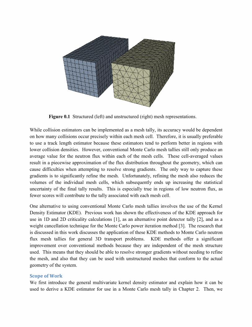
After the particle history for each neutron has been obtained, the next step in the Monte Carlo transport method is to assign a specific score to that history using an estimator. There are two main types of estimators that can be used to obtain the neutron flux within a 3D system. The first is the collision estimator, which assigns a score to the history every time a discrete collision event occurs. The second is the track length estimator, which uses the entire path traveled by the neutron to assign a score to the history. Both of these estimators can be implemented as a Monte Carlo mesh tally, which is used to accumulate all of the scores that fall within each mesh cell of some structured or unstructured mesh defined over all or part of the input geometry. Fig. 1.1 shows an example of both structured and unstructured mesh representations for a rectangular prism. Note that the 3D structured mesh is based on orthogonal hexahedra, whereas the 3D unstructured mesh consists of a set of tetrahedra. The primary advantage of using an unstructured mesh is because it can conform to non-orthogonal surfaces within the geometry. This conformal structure is useful when multiple materials are involved, since each tetrahedra within the mesh can be defined so that it only consists of a single material.

While collision estimators can be implemented as a mesh tally, its accuracy would be dependent on how many collisions occur precisely within each mesh cell. Therefore, it is usually preferable to use a track length estimator because these estimators tend to perform better in regions with lower collision densities. However, conventional Monte Carlo mesh tallies still only produce an average value for the neutron flux within each of the mesh cells. These cell-averaged values result in a piecewise approximation of the flux distribution throughout the geometry, which can cause difficulties when attempting to resolve strong gradients. The only way to capture these gradients is to significantly refine the mesh. Unfortunately, refining the mesh also reduces the volumes of the individual mesh cells, which subsequently ends up increasing the statistical uncertainty of the final tally results. This is especially true in regions of low neutron flux, as fewer scores will contribute to the tally associated with each mesh cell.

One alternative to using conventional Monte Carlo mesh tallies involves the use of the Kernel Density Estimator (KDE). Previous work has shown the effectiveness of the KDE approach for use in 1D and 2D criticality calculations [1], as an alternative point detector tally [2], and as a weight cancellation technique for the Monte Carlo power iteration method [3]. The research that is discussed in this work discusses the application of these KDE methods to Monte Carlo neutron flux mesh tallies for general 3D transport problems. KDE methods offer a significant improvement over conventional methods because they are independent of the mesh structure used. This means that they should be able to resolve stronger gradients without needing to refine the mesh, and also that they can be used with unstructured meshes that conform to the actual geometry of the system.

Scope of Work

We first introduce the general multivariate kernel density estimator and explain how it can be used to derive a KDE estimator for use in a Monte Carlo mesh tally in Chapter 2. Then, we

Figure 0.1 Structured (left) and unstructured (right) mesh representations.

provide a detailed discussion on some of the key issues that need to be considered in order to implement this alternative mesh tally within a production Monte Carlo transport code. In Chapter 3, we suggest how this new KDE mesh tally can be quantitatively compared to other mesh tally implementations for verification purposes. Then, in Chapter 4 we present the results of a bandwidth sensitivity experiment that was performed on this KDE mesh tally to see how this parameter affects the accuracy of its results. Finally, in Chapter 5 we provide a general summary of each of these chapters and discuss areas where more research is needed before mesh tallies based on a KDE approach can be considered a viable alternative to conventional mesh tallies.

KERNEL DENSITY ESTIMATED MONTE CARLO MESH TALLIES Density estimation is a group of statistical methods that attempt to reconstruct the shape of an unknown probability distribution from a finite set of observations sampled from that distribution. Parametric density estimation methods require that the general shape of the distribution is known a priori so that a theoretical function can be fit to the random sample by approximating its parameters. If the random sample is taken from a normal distribution, for example, then both the mean and variance would need to be estimated from this data so that a standard Gaussian function could then be used to reconstruct its shape. In many cases, however, the general shape of the distribution cannot be known a priori. This is when non-parametric methods, such as the Kernel Density Estimator (KDE), are preferred. Non-parametric density estimation methods do not need to assume a priori that the unknown probability distribution belongs to a specific family of distributions. These methods reconstruct the shape of the distribution directly from the random sample. Since the shape of a neutron flux distribution obtained using Monte Carlo methods is rarely known a priori, the KDE approach can be effectively used as an alternative to conventional estimators for determining the flux throughout some arbitrary geometric domain. This chapter first introduces the 3D kernel density estimator in Section 2.1. Then, in Section 2.2 we present the original KDE estimators that were developed as an alternative to conventional collision and track length estimators. Section 2.3 discusses the application of these estimators to mesh tallies, and explains why they can be ineffective for general 3D transport problems. In Section 2.4 we introduce a new KDE estimator based on integrated particle tracks. Finally, Section 2.5 discusses the implementation of this KDE integral-track estimator as a mesh tally.

Multivariate Kernel Density Estimator

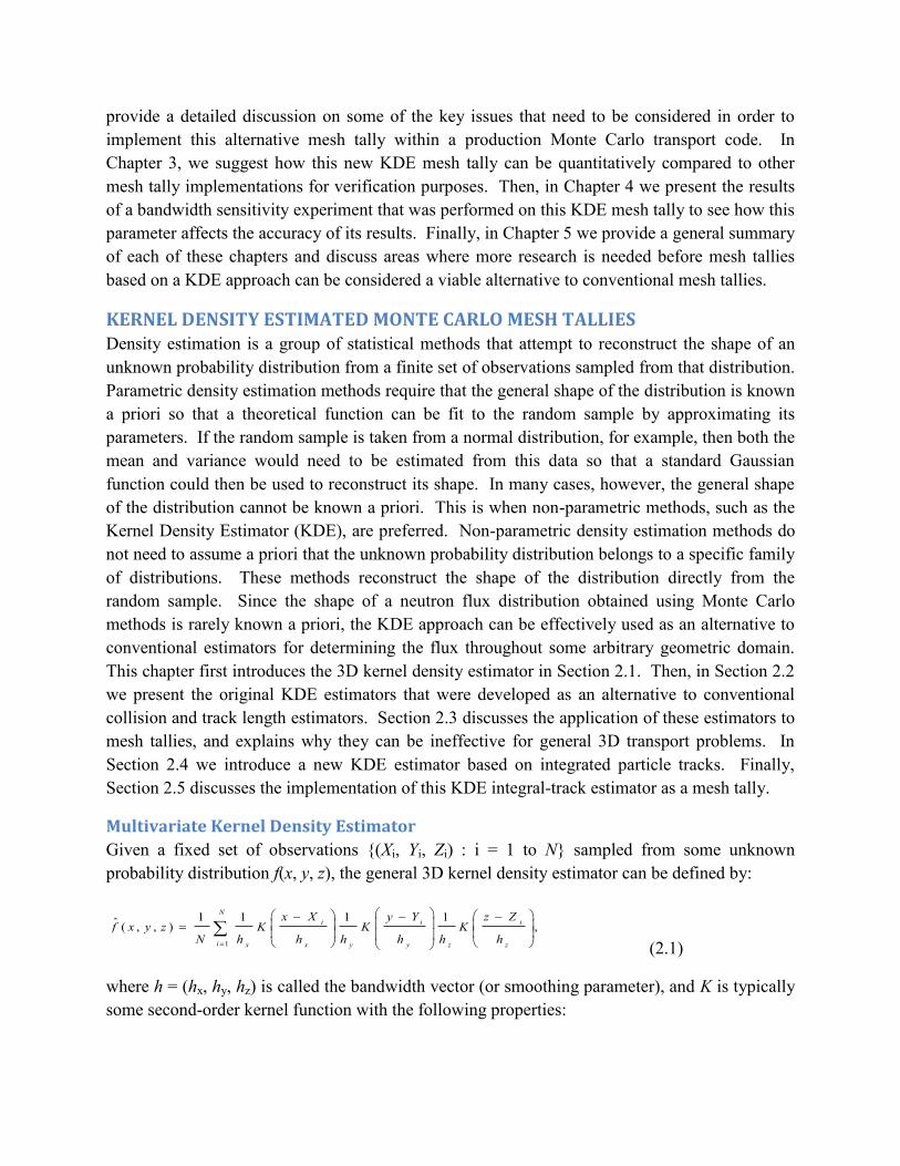
Given a fixed set of observations {(Xi, Yi, Zi) : i = 1 to N} sampled from some unknown probability distribution f(x, y, z), the general 3D kernel density estimator can be defined by:

N

i z

i

zy

i

yx

i

x h

ZzK

hh

YyK

hh

XxK

hNzyxf

1

,1111

),,(ˆ

(2.1)

where h = (hx, hy, hz) is called the bandwidth vector (or smoothing parameter), and K is typically some second-order kernel function with the following properties:

0)(.0)(.1)(.)()(. 2 duuKuduuuKduuKuKuK iviiiiii (2.2)

Based on a random sample taken from the unknown probability distribution being approximated, the kernel density estimator essentially places these kernel functions around each of the observations and adds them together to reconstruct the shape of the distribution. The bandwidth vector determines the width of the kernel functions in each dimension, whereas the shape of the kernel function determines how much each observation contributes to the total sum for some fixed calculation point (x, y, z).

Bandwidth

The choice of the bandwidth vector h that is used with Eq. 2.1 can have a substantial impact on the effectiveness of the approximation for the unknown probability distribution at all of the calculation points. A mathematical analysis concerning this issue has already been discussed in detail by Banerjee for general univariate and multivariate kernel density estimators [4]. Based on this analysis, it was shown that the choice of the bandwidth vector essentially comes down to a trade-off between variance and bias. Using smaller values minimizes the bias of the results at the cost of higher variance, whereas using larger values has the opposite effect. The optimal value falls somewhere in between these two extremes, and can be approximated for the general 3D kernel density estimator by:

,5

4,

5

4,

5

47/17/17/1

iii ZzYyXxN

hN

hN

h

(2.3)

where iX , iY and iZ are the standard deviations of the Xi, Yi and Zi components of the N observations that were used to approximate the unknown probability distribution.

Kernel function

In addition to the choice of the bandwidth vector, it is also necessary to decide what kernel function K to use when approximating an unknown probability distribution using Eq. 2.1. Two common kernel functions that can be used for density estimation purposes include the Uniform kernel:

,1,2

1)( uuK

(2.4)

and the rescaled Epanechnikov kernel:

.1),1(4

3)( 2

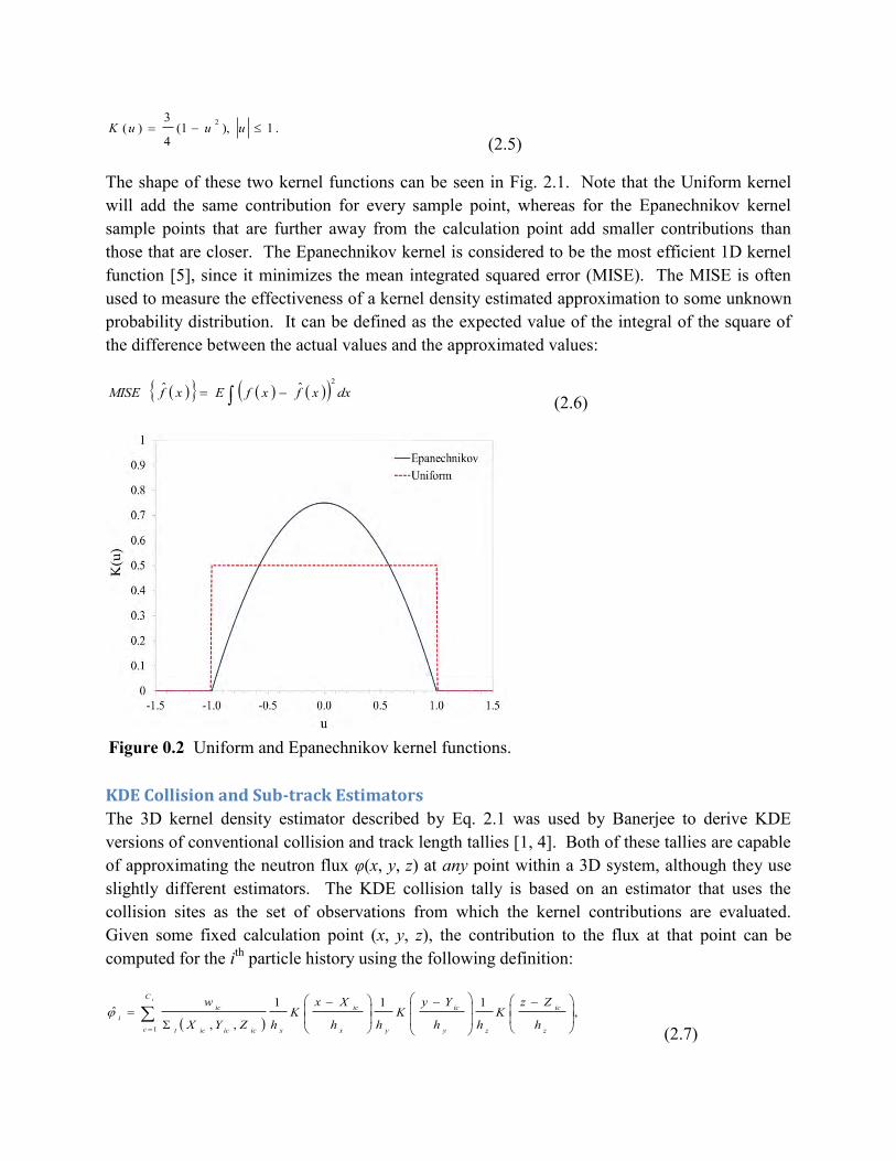
uuuK (2.5)

The shape of these two kernel functions can be seen in Fig. 2.1. Note that the Uniform kernel will add the same contribution for every sample point, whereas for the Epanechnikov kernel sample points that are further away from the calculation point add smaller contributions than those that are closer. The Epanechnikov kernel is considered to be the most efficient 1D kernel function [5], since it minimizes the mean integrated squared error (MISE). The MISE is often used to measure the effectiveness of a kernel density estimated approximation to some unknown probability distribution. It can be defined as the expected value of the integral of the square of the difference between the actual values and the approximated values:

dxxfxfExfMISE2ˆˆ

(2.6)

KDE Collision and Sub-track Estimators

The 3D kernel density estimator described by Eq. 2.1 was used by Banerjee to derive KDE versions of conventional collision and track length tallies [1, 4]. Both of these tallies are capable of approximating the neutron flux φ(x, y, z) at any point within a 3D system, although they use slightly different estimators. The KDE collision tally is based on an estimator that uses the collision sites as the set of observations from which the kernel contributions are evaluated. Given some fixed calculation point (x, y, z), the contribution to the flux at that point can be computed for the ith particle history using the following definition:

iC

c z

ic

zy

ic

yx

ic

xicicict

ici

h

ZzK

hh

YyK

hh

XxK

hZYX

w

1

,111

,,

(2.7)

Figure 0.2 Uniform and Epanechnikov kernel functions.

where Ci is the number of collision events experienced by the particle, wic is its weight, and Σt is the cross section of the material defined at the collision site (Xic, Yic, Zic).

Like conventional collision tallies, the KDE collision tally suffers in regions with low collision density and cannot be used at all in void regions. So, to be able to handle general 3D transport problems, it is usually preferable to use an estimator based on track length. As an alternative to using collision sites, the KDE track length tally developed by Banerjee is based on an estimator that chooses n pseudo-collision points (Xicj, Yicj, Zicj) along the track as the set of observations from which the individual kernel contributions Kicj are evaluated. These points are randomly selected by first splitting up the total track length dic into a series of n evenly distributed sub-tracks, and then by choosing one point within each region. The contribution to the flux for the ith particle history at some fixed calculation point (x, y, z) is then computed using an average of these individual kernel contributions as follows:

iC

c

n

jicjicici K

ndw

1 1

,1

(2.8)

where Kicj is defined as the product of three 1D kernel functions:

.111

z

icj

zy

icj

yx

icj

x

icjh

ZzK

hh

YyK

hh

XxK

hK

(2.9)

Applying Kernel Density Estimator Methods to Monte Carlo Mesh Tallies

Since the KDE collision and KDE sub-track estimators discussed in the previous section can approximate the neutron flux anywhere within some arbitrary geometric domain, it is possible to implement them both as an alternative Monte Carlo mesh tally. The main consideration that is needed to expand their usage to mesh tallies is to define the set of calculation points at which the kernel density estimator is to be evaluated. This makes the KDE approach well-suited to neutron flux tallies on unstructured meshes for two key reasons. First, the set of mesh nodes provides a useful set of calculation points to obtain a good representation of the entire flux distribution. In addition, unlike conventional mesh tallies, using the KDE approach does not require tracking particles across internal mesh boundaries and therefore is not affected by the size of the mesh cells. This means that refinement of the mesh to obtain higher fidelity results can be done by simply increasing the number of calculation points that are considered in the analysis, without having to worry about increased statistical error.

Even though both the KDE collision and sub-track estimators can be used to implement a mesh tally, the accuracy of their contributions depends on the either the collision density or the number of sub-tracks that are used. While the KDE sub-track estimator is preferable out of the two options, two few sub-tracks used with longer particle tracks could produce less accurate results – since only a small portion of the full track length is being considered. If this was the case, then a mesh tally based on the KDE sub-track estimator would not be much better than one based on

the KDE collision estimator. Even though it is easy enough to simply increase the number of sub-tracks that are used, for a three-dimensional mesh tally the neutron flux must be evaluated at numerous mesh nodes for each track segment. Using too many sub-tracks for these calculations could become expensive computationally, especially when considering large meshes that need to keep track of many particle histories. Therefore, a better approach is to consider an alternative KDE track length estimator that uses integrated particle tracks instead of pseudo-collisions for general transport problems defined on arbitrary unstructured meshes.

KDE Integral-track Estimator

The KDE integral-track estimator can be derived directly from the KDE sub-track estimator defined by Eq. 2.8 and 2.9. We first redefine the pseudo-collision points (Xicj, Yicj, Zicj) in terms of a common random path length variable Sicj:

icjoicjicjoicjicjoicj wSZZvSYYuSXX ... iiiiii (2.10)

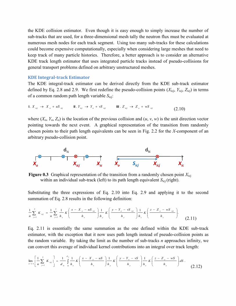
where (Xo, Yo, Zo) is the location of the previous collision and (u, v, w) is the unit direction vector pointing towards the next event. A graphical representation of the transition from randomly chosen points to their path length equivalents can be seen in Fig. 2.2 for the X-component of an arbitrary pseudo-collision point.

Substituting the three expressions of Eq. 2.10 into Eq. 2.9 and applying it to the second summation of Eq. 2.8 results in the following definition:

.11111

11

n

j z

icjo

zy

icjo

yx

icjo

x

n

jicj

h

wSZzK

hh

vSYyK

hh

uSXxK

hnK

n (2.11)

Eq. 2.11 is essentially the same summation as the one defined within the KDE sub-track estimator, with the exception that it now uses path length instead of pseudo-collision points as the random variable. By taking the limit as the number of sub-tracks n approaches infinity, we can convert this average of individual kernel contributions into an integral over track length:

.11111

lim01

dSh

wSZzK

hh

vSYyK

hh

uSXxK

hdK

n

icd

z

o

zy

o

yx

o

xic

n

jicj

n

(2.12)

Figure 0.3 Graphical representation of the transition from a randomly chosen point Xicj within an individual sub-track (left) to its path length equivalent Sicj (right).

Then, substituting Eq. 2.12 back into Eq. 2.8 and noting that the total track length term dic cancels, we obtain the final form of the KDE integral-track estimator:

i icC

c

d

Sici dSKw1 0

.

(2.13)

where KS is used to represent the following 3D kernel function as a function of path length S:

.111

z

o

zy

o

yx

o

x

Sh

wSZzK

hh

vSYyK

hh

uSXxK

hK

(2.14)

KDE Integral-track Mesh Tally Implementation

The KDE integral-track estimator defined by Eq. 2.13 and 2.14 has been implemented within the Direct Accelerated Geometry Monte Carlo N-Particle (DAG-MCNP) transport code [6] as an alternative mesh tally capable of using either structured or unstructured meshes. This new tally uses the following equations to compute the expected value of the neutron flux and its relative standard error at all of the mesh nodes (x, y, z) defined by some input mesh:

N

i

C

c

d

Sic

i ic

dSKwN

zyx1 1 0

,1

),,(

(2.15)

,),,(ˆ1

1

1 2

2

1 1 0

2),,(ˆ

zyxdSKwNN

N

i

C

c

d

Siczyx

i ic

(2.16)

where N is the number of particle histories that were used in the Monte Carlo simulation. These mesh nodes can be thought of as a series of fixed individual tally points or detectors, without the 1/R2 singularity that can cause issues with conventional point detector estimators [2]. As each track length dic is processed during the random walk, all mesh nodes within some neighborhood region around this track will add a new contribution to their corresponding tally sums. Nodes further from the track typically add smaller contributions than those closer to the track, depending on the kernel function that is used in the approximation.

Defining the neighborhood region

Since typical input meshes can have thousands of nodes, the concept of the neighborhood region for the KDE integral-track mesh tally is essential for efficiency purposes. This neighborhood region is defined as the local region in space around a single track for which the kernel function produces a non-trivial result for any mesh node inside that region. Even though most kernel functions are confined to a finite domain that ensures no contribution is ever added for mesh nodes outside this region, checking thousands of trivial calculation points per tally event can add

a significant penalty to the overall execution time. By limiting the number of nodes that are evaluated before any calculations are made, this penalty is kept to a minimum.

For a mesh tally based on the KDE collision estimator, defining the neighborhood region for a single collision is straightforward. An axis-aligned box is simply placed around the collision site, with its size determined only by the bandwidth that was used in the approximation. However, for a KDE integral-track mesh tally, attempting to define the exact neighborhood region becomes much more complicated because its size is determined by more than just the bandwidth. To make things even more difficult, the shape of this region is dependent on the orientation of the track segment with respect to its starting location. The simplest case occurs when the particle is traveling parallel to an axis, which produces a neighborhood region that is an axis-aligned box placed around the track segment. For the most challenging case, the particle is traveling in a direction that is not aligned with any axis. In this case, the neighborhood region would look something like the inner hexagonal shape shown in Fig. 2.3.

Because these neighborhood regions can get so complicated to define for an arbitrary track segment contributing to a KDE integral-track mesh tally, an approximation equivalent to the outer cubed region in Fig. 2.3 is used in the DAG-MCNP implementation instead. To determine a set of equations that describe the size of this approximated region, we first must restrict the 1D kernel functions to a finite domain. Both the Uniform and Epanechnikov kernels are already defined on the interval [-1, 1], which means that the following inequality must be satisfied in order to produce a non-zero tally contribution for the x-coordinate of the mesh node:

11

x

o

h

uSXx

(2.17)

Since Xo, u and hx are fixed for any given track segment, this means that x and S are the only unknowns. Rearranging Eq. 2.17 to focus on x, we get the following:

Figure 0.4 Sample neighborhood region for one track segment contributing to a KDE integral-track mesh tally.

uSXhxuSXh oxox (2.18)

Now note that the path length can range from S = 0 at the beginning of the track to S = dic at the end of the track. This means that if S = 0, then x must be within the interval [-hx + Xo, hx + Xo] to produce a non-trivial tally contribution. Similarly, if S = dic, then x needs to be within the interval [-hx + Xo + dicu, hx + Xo + dicu]. From these two extreme cases, we can construct the following valid ranges for x using the laws of inequalities to determine the minimum and maximum values:

.0 if ],[

,0 if ],[

,0 if ],[

uXhudXhx

uudXhXhx

uXhXhx

oxicox

icoxox

oxox

(2.19)

The procedure for determining the valid range of the x-coordinate that was just discussed can be easily extended to the other two dimensions. When combined, this set of three equations reduces the total number of mesh nodes into a much smaller set of calculation points that all fall within a simple axis-aligned box that encloses the track. Any mesh nodes that do not satisfy all three of these equations can be safely ignored as they are guaranteed to provide a zero contribution. However, while this crude approximation defines the exact neighborhood for a track that is aligned with an axis, for other track segments it may still include numerous trivial mesh nodes. As an alternative, it is possible to use a cylinder centered on the track instead. The maximum radius rmax of this cylinder can be computed from the bandwidth vector using the following formula:

.222max zyx hhhr

(2.20)

So, for each track segment the first step is to find all calculation points within the crude approximation. Then, the next step is to check each of these points against the radius of the cylinder defined by Eq. 2.20. Only points that fall within this radius should be added to the neighborhood region because all other points are guaranteed to produce a zero contribution. However, using this extra step will only be beneficial if more than half of the mesh nodes bounded by the box can be discarded due to being outside the cylinder. Since this depends on the orientation of the track segment, more research is needed to determine when it is more efficient to use rmax rather than simply relying on the crude approximation.

Choosing the integration limits

Once the set of mesh nodes within the neighborhood region has been determined for any given track segment, the next step is to compute the new contributions that will be added to the individual tally sums. These contributions are determined separately for each node by

integrating the kernel function KS with respect to the path length – treating the x, y, and z-coordinates of the mesh node being evaluated as constants. Before the integration step is performed on any given mesh node, however, the KDE integral-track mesh tally will first check for valid integration limits. Since the 3D kernel function is a product of 1D kernel functions, the entire integrand will be zero if any of these three terms evaluate to zero. Therefore, the choice of integration limits will depend on the interval S = [Smin, Smax] for which the 3D kernel function is non-zero. This may or may not be equivalent to the full track length, which is defined by the interval T = [0, dic]. If there is no region of overlap between S and T, then there are no valid integration limits and no further computations are needed. This will be the case for mesh nodes that fall outside the exact neighborhood region, but inside the crude approximation shown earlier in Fig. 2.3. Checking for valid integration limits for these nodes prevents these trivial integrations from being performed.

The procedure for choosing the integration limits is shown graphically in Fig. 2.4. First, valid ranges for each of the three dimensions (Sx, Sy, Sz) are determined. This can be done using Eq. 2.17 and solving for the path length variable S. For the x-coordinate, this results in the following set of equations for Sx:

.0 if ,S

,0 if ,S

,0 if ],0[S

x

x

x

uu

Xxh

u

Xxh

uu

Xxh

u

Xxh

ud

oxox

oxox

ic

(2.21)

Once valid ranges have been obtained for all three dimensions separately, the next step is to combine them into a common region of overlap to create the interval S. The lowest value of this region of overlap becomes Smin, whereas the highest value becomes Smax. After S has been defined, the final step is to compare this interval to the full track length. If S lies completely within T, such as in Fig. 2.4, then Smin and Smax become the lower and upper integration limits respectively. If Smin is less than zero, then the lower integration limit will be set to zero. Similarly, if Smax is greater than dic, then the upper integration limit will be set to dic.

Figure 0.5 Method for determining the integration limits of the path length integral.

Evaluating the path length integral

Suppose that valid integration limits were found for a specific mesh node within the neighborhood region. This means that it is guaranteed to add a non-zero contribution to its individual tally sum. To compute this contribution using the KDE integral-track estimator, we now need to evaluate the path length integral using the valid integration limits. The choice of integration method that will be the most effective depends on the kernel function that is used in the approximation. For the Epanechnikov kernel, which is the primary kernel implemented within DAG-MCNP, there is actually an analytical solution. However, this analytical solution consists of an anti-derivative that is a complicated 7th order polynomial. It takes over 120 arithmetic operations just to evaluate the largest of the eight terms in this polynomial once. Since the fundamental theorem of calculus requires that this anti-derivative be evaluated twice, this means that substantially more than 240 arithmetic operations would be needed for evaluating the path length integral at each mesh node with valid integration limits. Instead of using this computationally intensive analytical solution, all integrations performed by the KDE integral-track estimator in DAG-MCNP are based on a 4-point Gaussian quadrature method. This numerical method is guaranteed to provide exact results for all polynomials up to and including 7th order, which means that it can compute the exact path length integral when the Epanechnikov kernel is used in the approximation. In addition, this method only requires a total of around 124 arithmetic operations per mesh node, making it much more efficient than the analytical solution. One final advantage of the 4-point Gaussian quadrature method is that it can also be used effectively with other kernel functions, not just the Epanechnikov kernel.

Choosing a bandwidth value

Like other applications that use KDE methods, the KDE integral-track mesh tally is highly dependent on the choice of bandwidth. This choice of bandwidth affects both the size of the neighborhood region and the interval that defines the valid integration limits for each mesh node. Using smaller values means that each track segment contributes to fewer mesh nodes, which can increase the variance of the results. On the other hand, using larger values means that each track segment contributes to too many mesh nodes, potentially hiding important features of the underlying flux distribution due to increased bias in the results. While the optimal bandwidth can in theory be computed using Eq. 2.3 during a Monte Carlo simulation with minimal storage requirements, it cannot be used to obtain the tally results for a general 3D transport problem until the entire simulation is completed. As a result, it was decided to require that the user of the KDE integral-track mesh tally within DAG-MCNP choose a value for the bandwidth a priori. The effect that this choice can have on the tally results will be the main focus of Chapter 4.

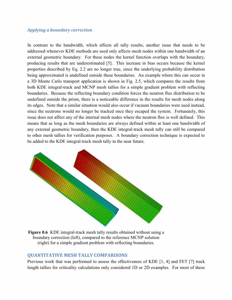
Applying a boundary correction

In contrast to the bandwidth, which affects all tally results, another issue that needs to be addressed whenever KDE methods are used only affects mesh nodes within one bandwidth of an external geometric boundary. For these nodes the kernel function overlaps with the boundary, producing results that are underestimated [5]. This increase in bias occurs because the kernel properties described by Eq. 2.2 are no longer true, since the underlying probability distribution being approximated is undefined outside these boundaries. An example where this can occur in a 3D Monte Carlo transport application is shown in Fig. 2.5, which compares the results from both KDE integral-track and MCNP mesh tallies for a simple gradient problem with reflecting boundaries. Because the reflecting boundary condition forces the neutron flux distribution to be undefined outside the prism, there is a noticeable difference in the results for mesh nodes along its edges. Note that a similar situation would also occur if vacuum boundaries were used instead, since the neutrons would no longer be tracked once they escaped the system. Fortunately, this issue does not affect any of the internal mesh nodes where the neutron flux is well defined. This means that as long as the mesh boundaries are always defined within at least one bandwidth of any external geometric boundary, then the KDE integral-track mesh tally can still be compared to other mesh tallies for verification purposes. A boundary correction technique is expected to be added to the KDE integral-track mesh tally in the near future.

QUANTITATIVE MESH TALLY COMPARISONS Previous work that was performed to assess the effectiveness of KDE [1, 4] and FET [7] track length tallies for criticality calculations only considered 1D or 2D examples. For most of these

Figure 0.6 KDE integral-track mesh tally results obtained without using a boundary correction (left), compared to the reference MCNP solution

(right) for a simple gradient problem with reflecting boundaries.

cases, a qualitative graphical analysis was used to show that their results were visually equivalent to some reference MCNP solution. However, for 3D problems it is preferable to use a more quantitative approach because the entire domain cannot be represented by a single graphic. Quantitatively comparing the KDE integral-track mesh tally to its predecessor is simple because they both approximate the flux at the mesh nodes. Unfortunately, things get more complicated when attempting to compare these nodal-based results to the cell-averaged results of a more conventional mesh tally because a data transfer method is needed. A similar issue arose when Griesheimer compared FET track length and MCNP mesh tally results for a 2D numerical example based on a single pin cell within an infinite lattice [7]. For this example, the continuous FET approximation was quantitatively compared to MCNP by first averaging the functional expansion over each mesh cell, and then by computing the relative difference between the two sets of results. In this chapter, we discuss in detail how quantitative mesh tally comparisons such as these can be performed on KDE integral-track mesh tally results. First, in Section 3.1 we introduce the conventions and definitions that will be used. Then, in Section 3.2 we describe a series of five verification test cases designed to show that the KDE integral-track mesh tally can produce equivalent results to other mesh tally implementations. These five test cases were used to quantitatively compare the KDE integral-track mesh tally to KDE sub-track and MCNP mesh tallies in Sections 3.3 and 3.5 respectively. Before presenting the results of the KDE versus MCNP mesh tally comparison, in Section 3.4 we consider some key issues that arise whenever nodal-based results are quantitatively compared to cell-averaged results.

Conventions for Quantitative Mesh Tally Comparisons

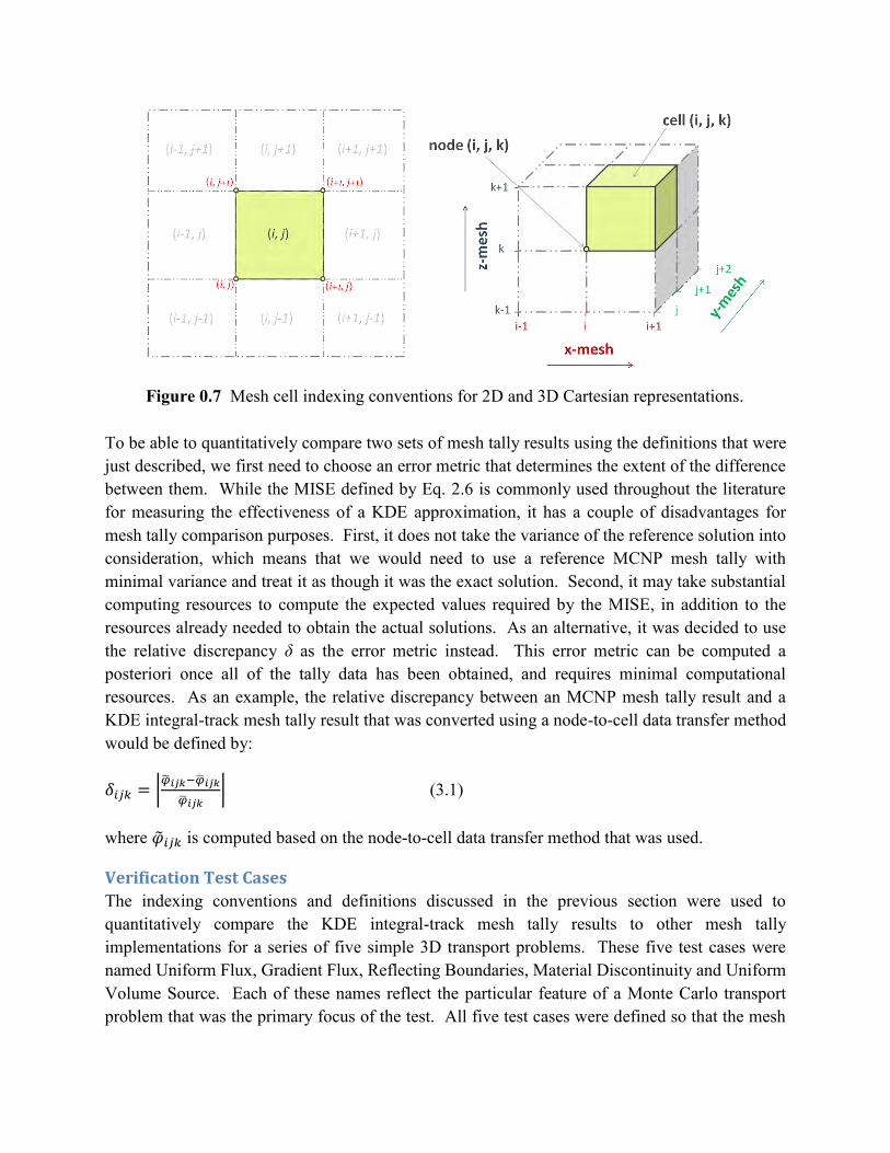
The indexing conventions used in this chapter to describe a quantitative tally comparison on 2D and 3D structured Cartesian meshes can be seen in Fig. 3.1. For the 2D case, the node at the bottom-left of cell (i, j) is defined as node (i, j). Similarly, node (i, j, k) is defined as the node at the front-bottom-left of cell (i, j, k) for the 3D case. An equivalent indexing convention will be used for 3D tetrahedral meshes. Based on these conventions, represents either a KDE sub-track or KDE integral-track mesh tally result at node (i, j, k), whereas represents an MCNP mesh tally result at cell (i, j, k). The subscript g refers to the energy group being considered, if applicable. If a data transfer method is used to convert from node-to-cell or cell-to-node results, then the original accent is replaced by a tilde for all mesh tallies: .

To be able to quantitatively compare two sets of mesh tally results using the definitions that were just described, we first need to choose an error metric that determines the extent of the difference between them. While the MISE defined by Eq. 2.6 is commonly used throughout the literature for measuring the effectiveness of a KDE approximation, it has a couple of disadvantages for mesh tally comparison purposes. First, it does not take the variance of the reference solution into consideration, which means that we would need to use a reference MCNP mesh tally with minimal variance and treat it as though it was the exact solution. Second, it may take substantial computing resources to compute the expected values required by the MISE, in addition to the resources already needed to obtain the actual solutions. As an alternative, it was decided to use the relative discrepancy δ as the error metric instead. This error metric can be computed a posteriori once all of the tally data has been obtained, and requires minimal computational resources. As an example, the relative discrepancy between an MCNP mesh tally result and a KDE integral-track mesh tally result that was converted using a node-to-cell data transfer method would be defined by:

|

| (3.1)

where is computed based on the node-to-cell data transfer method that was used.

Verification Test Cases

The indexing conventions and definitions discussed in the previous section were used to quantitatively compare the KDE integral-track mesh tally results to other mesh tally implementations for a series of five simple 3D transport problems. These five test cases were named Uniform Flux, Gradient Flux, Reflecting Boundaries, Material Discontinuity and Uniform Volume Source. Each of these names reflect the particular feature of a Monte Carlo transport problem that was the primary focus of the test. All five test cases were defined so that the mesh

Figure 0.7 Mesh cell indexing conventions for 2D and 3D Cartesian representations.

tally region of interest was within at least one bandwidth of any external geometric boundary to avoid needing to consider a boundary correction technique.

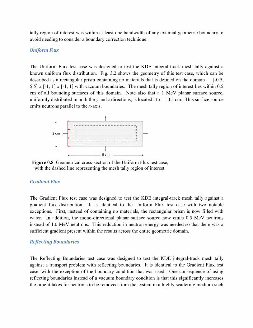
Uniform Flux

The Uniform Flux test case was designed to test the KDE integral-track mesh tally against a known uniform flux distribution. Fig. 3.2 shows the geometry of this test case, which can be described as a rectangular prism containing no materials that is defined on the domain [-0.5, 5.5] x [-1, 1] x [-1, 1] with vacuum boundaries. The mesh tally region of interest lies within 0.5 cm of all bounding surfaces of this domain. Note also that a 1 MeV planar surface source, uniformly distributed in both the y and z directions, is located at x = -0.5 cm. This surface source emits neutrons parallel to the x-axis.

Gradient Flux

The Gradient Flux test case was designed to test the KDE integral-track mesh tally against a gradient flux distribution. It is identical to the Uniform Flux test case with two notable exceptions. First, instead of containing no materials, the rectangular prism is now filled with water. In addition, the mono-directional planar surface source now emits 0.5 MeV neutrons instead of 1.0 MeV neutrons. This reduction in neutron energy was needed so that there was a sufficient gradient present within the results across the entire geometric domain.

Reflecting Boundaries

The Reflecting Boundaries test case was designed to test the KDE integral-track mesh tally against a transport problem with reflecting boundaries. It is identical to the Gradient Flux test case, with the exception of the boundary condition that was used. One consequence of using reflecting boundaries instead of a vacuum boundary condition is that this significantly increases the time it takes for neutrons to be removed from the system in a highly scattering medium such

Figure 0.8 Geometrical cross-section of the Uniform Flux test case, with the dashed line representing the mesh tally region of interest.

as water. To minimize this increase in computing time, the energy of the neutrons emitted by the mono-directional planar surface source was reduced from 0.5 MeV to 0.05 MeV.

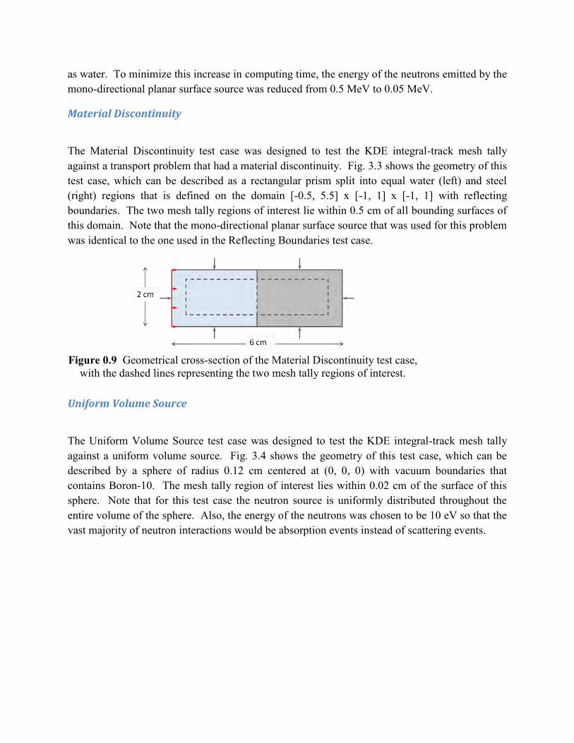
Material Discontinuity

The Material Discontinuity test case was designed to test the KDE integral-track mesh tally against a transport problem that had a material discontinuity. Fig. 3.3 shows the geometry of this test case, which can be described as a rectangular prism split into equal water (left) and steel (right) regions that is defined on the domain [-0.5, 5.5] x [-1, 1] x [-1, 1] with reflecting boundaries. The two mesh tally regions of interest lie within 0.5 cm of all bounding surfaces of this domain. Note that the mono-directional planar surface source that was used for this problem was identical to the one used in the Reflecting Boundaries test case.

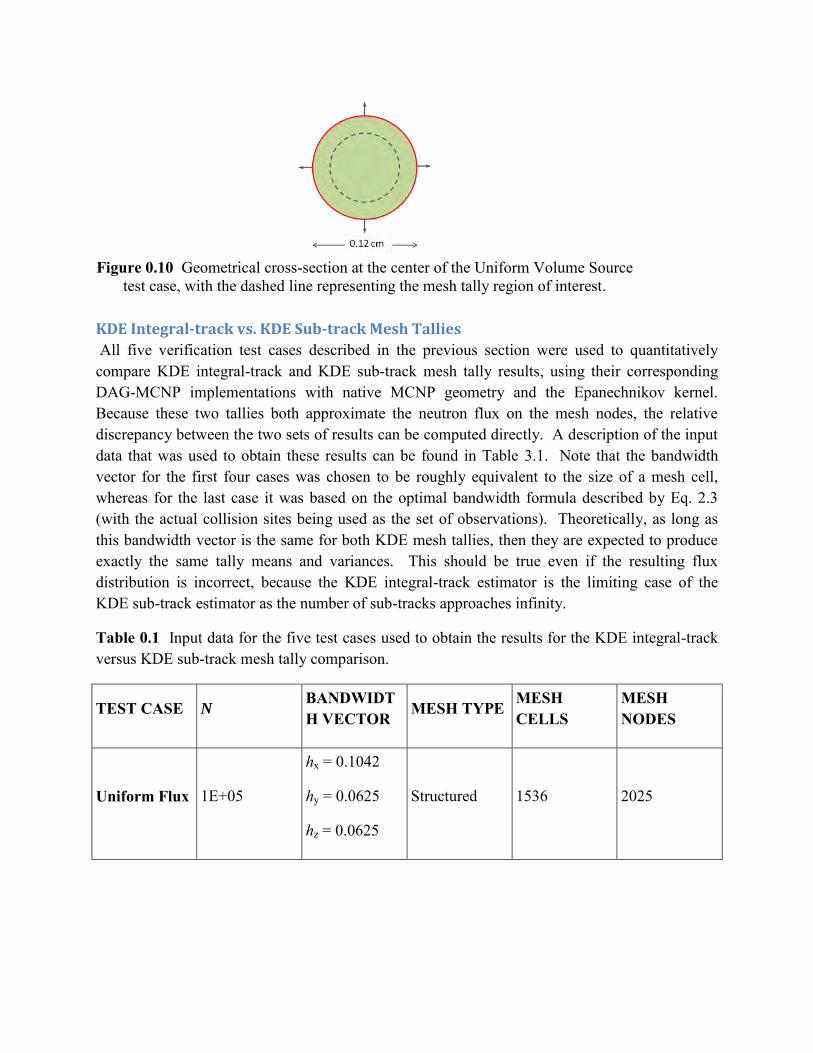
Uniform Volume Source

The Uniform Volume Source test case was designed to test the KDE integral-track mesh tally against a uniform volume source. Fig. 3.4 shows the geometry of this test case, which can be described by a sphere of radius 0.12 cm centered at (0, 0, 0) with vacuum boundaries that contains Boron-10. The mesh tally region of interest lies within 0.02 cm of the surface of this sphere. Note that for this test case the neutron source is uniformly distributed throughout the entire volume of the sphere. Also, the energy of the neutrons was chosen to be 10 eV so that the vast majority of neutron interactions would be absorption events instead of scattering events.

Figure 0.9 Geometrical cross-section of the Material Discontinuity test case, with the dashed lines representing the two mesh tally regions of interest.

KDE Integral-track vs. KDE Sub-track Mesh Tallies

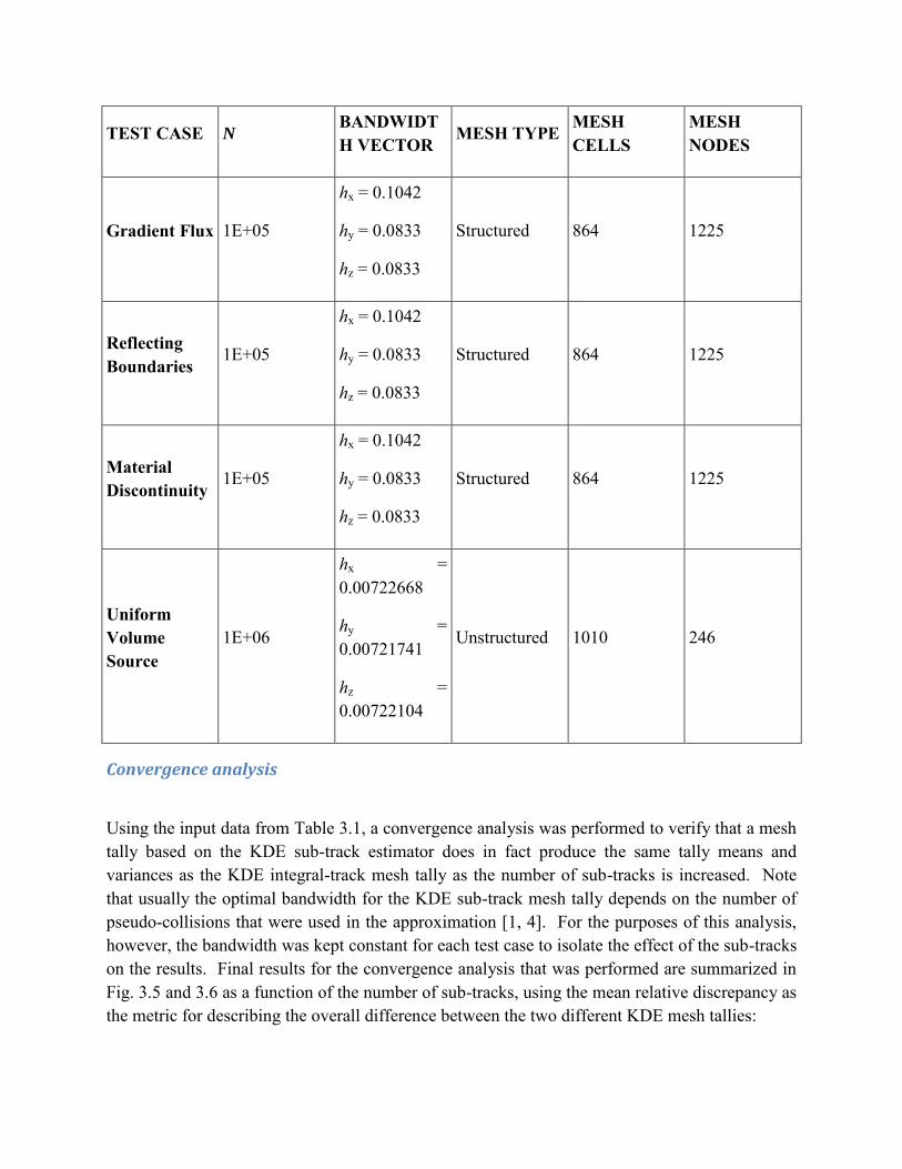
All five verification test cases described in the previous section were used to quantitatively compare KDE integral-track and KDE sub-track mesh tally results, using their corresponding DAG-MCNP implementations with native MCNP geometry and the Epanechnikov kernel. Because these two tallies both approximate the neutron flux on the mesh nodes, the relative discrepancy between the two sets of results can be computed directly. A description of the input data that was used to obtain these results can be found in Table 3.1. Note that the bandwidth vector for the first four cases was chosen to be roughly equivalent to the size of a mesh cell, whereas for the last case it was based on the optimal bandwidth formula described by Eq. 2.3 (with the actual collision sites being used as the set of observations). Theoretically, as long as this bandwidth vector is the same for both KDE mesh tallies, then they are expected to produce exactly the same tally means and variances. This should be true even if the resulting flux distribution is incorrect, because the KDE integral-track estimator is the limiting case of the KDE sub-track estimator as the number of sub-tracks approaches infinity.

Table 0.1 Input data for the five test cases used to obtain the results for the KDE integral-track versus KDE sub-track mesh tally comparison.

TEST CASE N BANDWIDTH VECTOR MESH TYPE MESH

CELLS MESH NODES

Uniform Flux 1E+05

hx = 0.1042

hy = 0.0625

hz = 0.0625

Structured 1536 2025

Figure 0.10 Geometrical cross-section at the center of the Uniform Volume Source test case, with the dashed line representing the mesh tally region of interest.

TEST CASE N BANDWIDTH VECTOR

MESH TYPE MESH CELLS

MESH NODES

Gradient Flux 1E+05

hx = 0.1042

hy = 0.0833

hz = 0.0833

Structured 864 1225

Reflecting Boundaries

1E+05

hx = 0.1042

hy = 0.0833

hz = 0.0833

Structured 864 1225

Material Discontinuity

1E+05

hx = 0.1042

hy = 0.0833

hz = 0.0833

Structured 864 1225

Uniform Volume Source

1E+06

hx = 0.00722668

hy = 0.00721741

hz = 0.00722104

Unstructured 1010 246

Convergence analysis

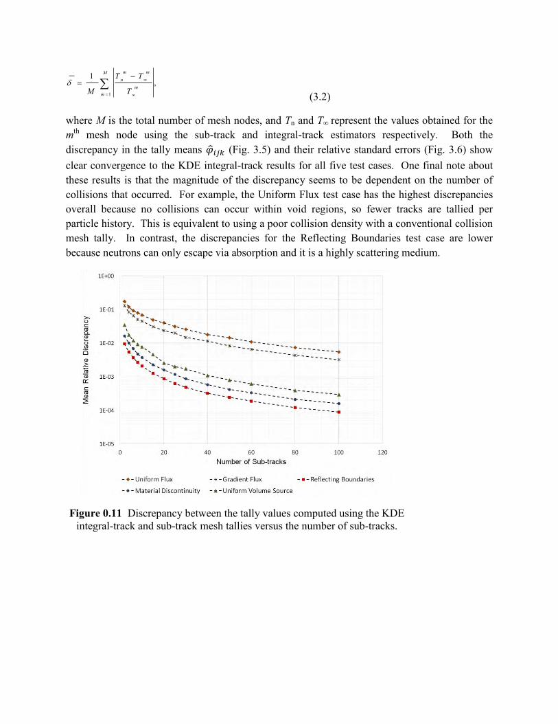
Using the input data from Table 3.1, a convergence analysis was performed to verify that a mesh tally based on the KDE sub-track estimator does in fact produce the same tally means and variances as the KDE integral-track mesh tally as the number of sub-tracks is increased. Note that usually the optimal bandwidth for the KDE sub-track mesh tally depends on the number of pseudo-collisions that were used in the approximation [1, 4]. For the purposes of this analysis, however, the bandwidth was kept constant for each test case to isolate the effect of the sub-tracks on the results. Final results for the convergence analysis that was performed are summarized in Fig. 3.5 and 3.6 as a function of the number of sub-tracks, using the mean relative discrepancy as the metric for describing the overall difference between the two different KDE mesh tallies:

M

mm

mmn

T

TT

M 1

,1

(3.2)

where M is the total number of mesh nodes, and Tn and T∞ represent the values obtained for the mth mesh node using the sub-track and integral-track estimators respectively. Both the discrepancy in the tally means (Fig. 3.5) and their relative standard errors (Fig. 3.6) show clear convergence to the KDE integral-track results for all five test cases. One final note about these results is that the magnitude of the discrepancy seems to be dependent on the number of collisions that occurred. For example, the Uniform Flux test case has the highest discrepancies overall because no collisions can occur within void regions, so fewer tracks are tallied per particle history. This is equivalent to using a poor collision density with a conventional collision mesh tally. In contrast, the discrepancies for the Reflecting Boundaries test case are lower because neutrons can only escape via absorption and it is a highly scattering medium.

Figure 0.11 Discrepancy between the tally values computed using the KDE integral-track and sub-track mesh tallies versus the number of sub-tracks.

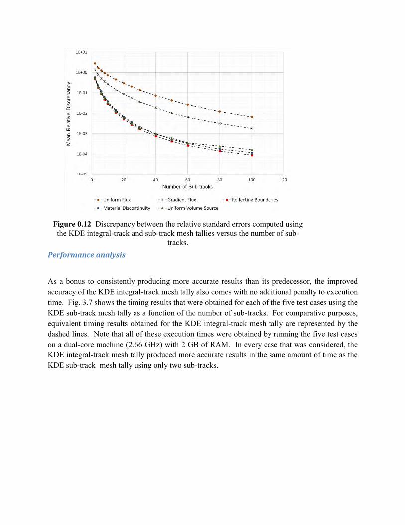
Performance analysis

As a bonus to consistently producing more accurate results than its predecessor, the improved accuracy of the KDE integral-track mesh tally also comes with no additional penalty to execution time. Fig. 3.7 shows the timing results that were obtained for each of the five test cases using the KDE sub-track mesh tally as a function of the number of sub-tracks. For comparative purposes, equivalent timing results obtained for the KDE integral-track mesh tally are represented by the dashed lines. Note that all of these execution times were obtained by running the five test cases on a dual-core machine (2.66 GHz) with 2 GB of RAM. In every case that was considered, the KDE integral-track mesh tally produced more accurate results in the same amount of time as the KDE sub-track mesh tally using only two sub-tracks.

Figure 0.12 Discrepancy between the relative standard errors computed using the KDE integral-track and sub-track mesh tallies versus the number of sub-

tracks.

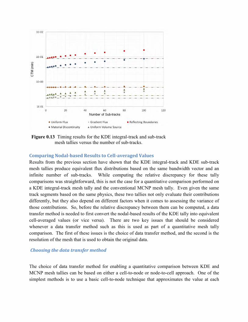
Comparing Nodal-based Results to Cell-averaged Values

Results from the previous section have shown that the KDE integral-track and KDE sub-track mesh tallies produce equivalent flux distributions based on the same bandwidth vector and an infinite number of sub-tracks. While computing the relative discrepancy for these tally comparisons was straightforward, this is not the case for a quantitative comparison performed on a KDE integral-track mesh tally and the conventional MCNP mesh tally. Even given the same track segments based on the same physics, these two tallies not only evaluate their contributions differently, but they also depend on different factors when it comes to assessing the variance of those contributions. So, before the relative discrepancy between them can be computed, a data transfer method is needed to first convert the nodal-based results of the KDE tally into equivalent cell-averaged values (or vice versa). There are two key issues that should be considered whenever a data transfer method such as this is used as part of a quantitative mesh tally comparison. The first of these issues is the choice of data transfer method, and the second is the resolution of the mesh that is used to obtain the original data.

Choosing the data transfer method

The choice of data transfer method for enabling a quantitative comparison between KDE and MCNP mesh tallies can be based on either a cell-to-node or node-to-cell approach. One of the simplest methods is to use a basic cell-to-node technique that approximates the value at each

Figure 0.13 Timing results for the KDE integral-track and sub-track mesh tallies versus the number of sub-tracks.

mesh node (i, j, k) by averaging the neutron flux for all mesh cells adjacent to that node. For a structured 3D Cartesian mesh, this would be computed by:

∑ ∑ ∑

(3.3)

where aijk is the number of cells that was used in the approximation. If Eq. 3.3 was used to estimate the nodal-based flux at an internal mesh node, then eight mesh cells would be included. However, if the same equation was used for a boundary node, then only up to four mesh cells would be included. This can introduce significant errors into the relative discrepancy calculations, especially if those boundary nodes are at the corners of the mesh.

As an alternative to this basic cell-to-node approach, a more effective method is to use a node-to-cell technique that makes use of finite element theory. A finite element can be thought of as a geometrical construct that is uniquely defined by its shape and a fixed number of nodes. Some common finite element representations for both hexahedral and tetrahedral geometries are

shown in Fig 3.8. Suppose that the flux k is known at all n nodes of a mesh cell that can also be defined as a 3D finite element. Given these values, the flux at any other point within the mesh cell can be approximated by the interpolation function [8]:

,),,(ˆ),,(ˆ1

321321

n

kkk N

(3.4)

where Nk is the basis function at the kth node of the element, expressed in terms of its natural coordinates (ξ1, ξ2, ξ3). Using Eq. 3.4 to approximate the flux at the p cubature points of a Gaussian cubature rule, the cell-averaged flux for the mesh cell can then be estimated by:

,ˆ1

),,(

),,(~

1 1

p

l

n

k

lkk

ll

V

V NjwV

dV

dVzyx

zyx

(3.5)

where the superscript l refers to the natural coordinates of the lth cubature point, w is the cubature weight, j is the determinant of the Jacobian matrix, and V is the volume of the mesh cell.

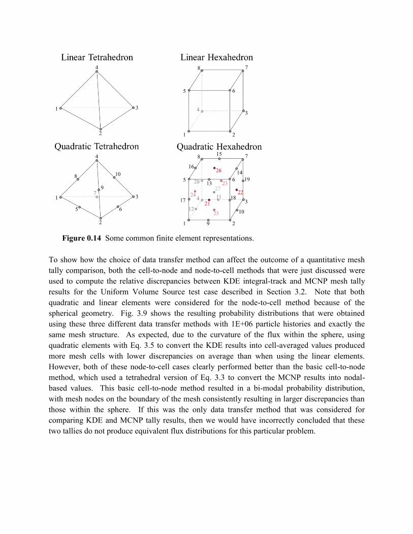
To show how the choice of data transfer method can affect the outcome of a quantitative mesh tally comparison, both the cell-to-node and node-to-cell methods that were just discussed were used to compute the relative discrepancies between KDE integral-track and MCNP mesh tally results for the Uniform Volume Source test case described in Section 3.2. Note that both quadratic and linear elements were considered for the node-to-cell method because of the spherical geometry. Fig. 3.9 shows the resulting probability distributions that were obtained using these three different data transfer methods with 1E+06 particle histories and exactly the same mesh structure. As expected, due to the curvature of the flux within the sphere, using quadratic elements with Eq. 3.5 to convert the KDE results into cell-averaged values produced more mesh cells with lower discrepancies on average than when using the linear elements. However, both of these node-to-cell cases clearly performed better than the basic cell-to-node method, which used a tetrahedral version of Eq. 3.3 to convert the MCNP results into nodal-based values. This basic cell-to-node method resulted in a bi-modal probability distribution, with mesh nodes on the boundary of the mesh consistently resulting in larger discrepancies than those within the sphere. If this was the only data transfer method that was considered for comparing KDE and MCNP tally results, then we would have incorrectly concluded that these two tallies do not produce equivalent flux distributions for this particular problem.

Figure 0.14 Some common finite element representations.

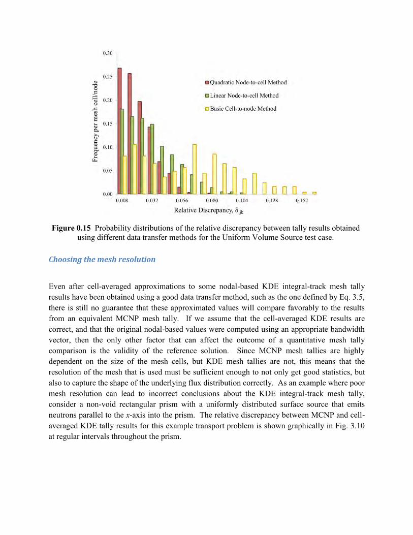
Choosing the mesh resolution

Even after cell-averaged approximations to some nodal-based KDE integral-track mesh tally results have been obtained using a good data transfer method, such as the one defined by Eq. 3.5, there is still no guarantee that these approximated values will compare favorably to the results from an equivalent MCNP mesh tally. If we assume that the cell-averaged KDE results are correct, and that the original nodal-based values were computed using an appropriate bandwidth vector, then the only other factor that can affect the outcome of a quantitative mesh tally comparison is the validity of the reference solution. Since MCNP mesh tallies are highly dependent on the size of the mesh cells, but KDE mesh tallies are not, this means that the resolution of the mesh that is used must be sufficient enough to not only get good statistics, but also to capture the shape of the underlying flux distribution correctly. As an example where poor mesh resolution can lead to incorrect conclusions about the KDE integral-track mesh tally, consider a non-void rectangular prism with a uniformly distributed surface source that emits neutrons parallel to the x-axis into the prism. The relative discrepancy between MCNP and cell-averaged KDE tally results for this example transport problem is shown graphically in Fig. 3.10 at regular intervals throughout the prism.

Figure 0.15 Probability distributions of the relative discrepancy between tally results obtained using different data transfer methods for the Uniform Volume Source test case.

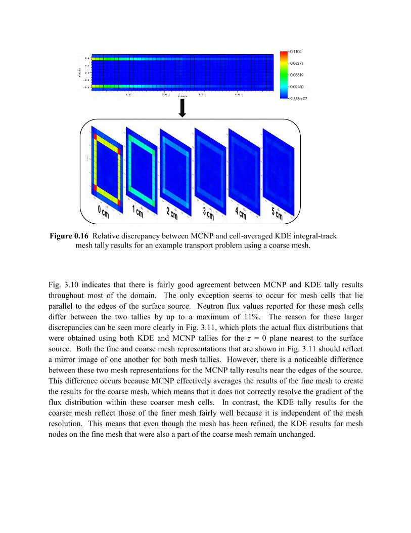
Fig. 3.10 indicates that there is fairly good agreement between MCNP and KDE tally results throughout most of the domain. The only exception seems to occur for mesh cells that lie parallel to the edges of the surface source. Neutron flux values reported for these mesh cells differ between the two tallies by up to a maximum of 11%. The reason for these larger discrepancies can be seen more clearly in Fig. 3.11, which plots the actual flux distributions that were obtained using both KDE and MCNP tallies for the z = 0 plane nearest to the surface source. Both the fine and coarse mesh representations that are shown in Fig. 3.11 should reflect a mirror image of one another for both mesh tallies. However, there is a noticeable difference between these two mesh representations for the MCNP tally results near the edges of the source. This difference occurs because MCNP effectively averages the results of the fine mesh to create the results for the coarse mesh, which means that it does not correctly resolve the gradient of the flux distribution within these coarser mesh cells. In contrast, the KDE tally results for the coarser mesh reflect those of the finer mesh fairly well because it is independent of the mesh resolution. This means that even though the mesh has been refined, the KDE results for mesh nodes on the fine mesh that were also a part of the coarse mesh remain unchanged.

Figure 0.16 Relative discrepancy between MCNP and cell-averaged KDE integral-track mesh tally results for an example transport problem using a coarse mesh.

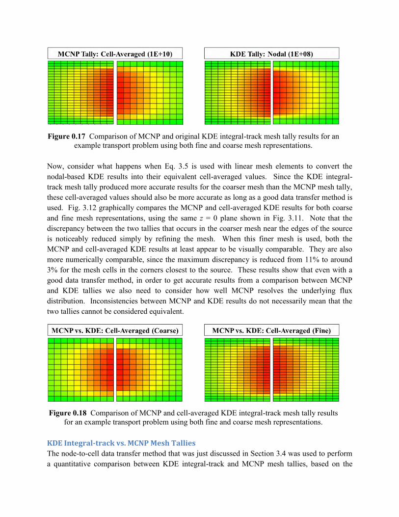
Now, consider what happens when Eq. 3.5 is used with linear mesh elements to convert the nodal-based KDE results into their equivalent cell-averaged values. Since the KDE integral-track mesh tally produced more accurate results for the coarser mesh than the MCNP mesh tally, these cell-averaged values should also be more accurate as long as a good data transfer method is used. Fig. 3.12 graphically compares the MCNP and cell-averaged KDE results for both coarse and fine mesh representations, using the same z = 0 plane shown in Fig. 3.11. Note that the discrepancy between the two tallies that occurs in the coarser mesh near the edges of the source is noticeably reduced simply by refining the mesh. When this finer mesh is used, both the MCNP and cell-averaged KDE results at least appear to be visually comparable. They are also more numerically comparable, since the maximum discrepancy is reduced from 11% to around 3% for the mesh cells in the corners closest to the source. These results show that even with a good data transfer method, in order to get accurate results from a comparison between MCNP and KDE tallies we also need to consider how well MCNP resolves the underlying flux distribution. Inconsistencies between MCNP and KDE results do not necessarily mean that the two tallies cannot be considered equivalent.

KDE Integral-track vs. MCNP Mesh Tallies

The node-to-cell data transfer method that was just discussed in Section 3.4 was used to perform a quantitative comparison between KDE integral-track and MCNP mesh tallies, based on the

Figure 0.17 Comparison of MCNP and original KDE integral-track mesh tally results for an example transport problem using both fine and coarse mesh representations.

Figure 0.18 Comparison of MCNP and cell-averaged KDE integral-track mesh tally results for an example transport problem using both fine and coarse mesh representations.

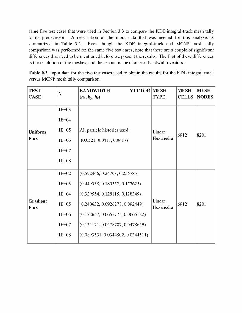
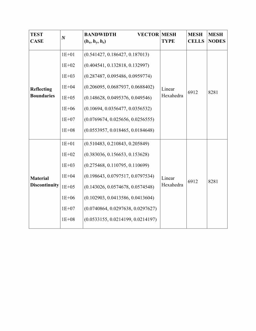
same five test cases that were used in Section 3.3 to compare the KDE integral-track mesh tally to its predecessor. A description of the input data that was needed for this analysis is summarized in Table 3.2. Even though the KDE integral-track and MCNP mesh tally comparison was performed on the same five test cases, note that there are a couple of significant differences that need to be mentioned before we present the results. The first of these differences is the resolution of the meshes, and the second is the choice of bandwidth vectors.

Table 0.2 Input data for the five test cases used to obtain the results for the KDE integral-track versus MCNP mesh tally comparison.

TEST CASE N

BANDWIDTH VECTOR (hx, hy, hz)

MESH TYPE

MESH CELLS

MESH NODES

Uniform Flux

1E+03

1E+04

1E+05

1E+06

1E+07

1E+08

All particle histories used:

(0.0521, 0.0417, 0.0417)

Linear Hexahedra

6912 8281

Gradient Flux

1E+02

1E+03

1E+04

1E+05

1E+06

1E+07

1E+08

(0.592466, 0.24703, 0.256785)

(0.449338, 0.180352, 0.177625)

(0.329554, 0.128115, 0.128349)

(0.240632, 0.0926277, 0.092449)

(0.172657, 0.0665775, 0.0665122)

(0.124171, 0.0478787, 0.0478659)

(0.0893531, 0.0344502, 0.0344511)

Linear Hexahedra

6912 8281

TEST CASE

N BANDWIDTH VECTOR (hx, hy, hz)

MESH TYPE

MESH CELLS

MESH NODES

Reflecting Boundaries

1E+01

1E+02

1E+03

1E+04

1E+05

1E+06

1E+07

1E+08

(0.541427, 0.186427, 0.187013)

(0.404541, 0.132818, 0.132997)

(0.287487, 0.095486, 0.0959774)

(0.206095, 0.0687937, 0.0688402)

(0.148628, 0.0495376, 0.049546)

(0.10694, 0.0356477, 0.0356532)

(0.0769674, 0.025656, 0.0256555)

(0.0553957, 0.018465, 0.0184648)

Linear Hexahedra

6912 8281

Material Discontinuity

1E+01

1E+02

1E+03

1E+04

1E+05

1E+06

1E+07

1E+08

(0.510483, 0.210843, 0.205849)

(0.383036, 0.156653, 0.153628)

(0.275468, 0.110795, 0.110699)

(0.198643, 0.0797517, 0.0797534)

(0.143026, 0.0574678, 0.0574548)

(0.102903, 0.0413586, 0.0413604)

(0.0740864, 0.0297638, 0.0297627)

(0.0533155, 0.0214199, 0.0214197)

Linear Hexahedra

6912 8281

TEST CASE

N BANDWIDTH VECTOR (hx, hy, hz)

MESH TYPE

MESH CELLS

MESH NODES

Uniform Volume Source

1E+02

1E+03

1E+04

1E+05

1E+06

1E+07

1E+08

(0.0258763, 0.0261472, 0.0284612)

(0.0200247, 0.0193893, 0.0193136)

(0.0139877, 0.0139137, 0.0139136)

(0.0100222, 0.0100461, 0.0100493)

(0.00722668, 0.00721741, 0.00722104)

(0.00519784, 0.00519823, 0.00519855)

(0.00374131, 0.00374109, 0.00374135)

Quadratic Tetrahedra

47,039 67,331

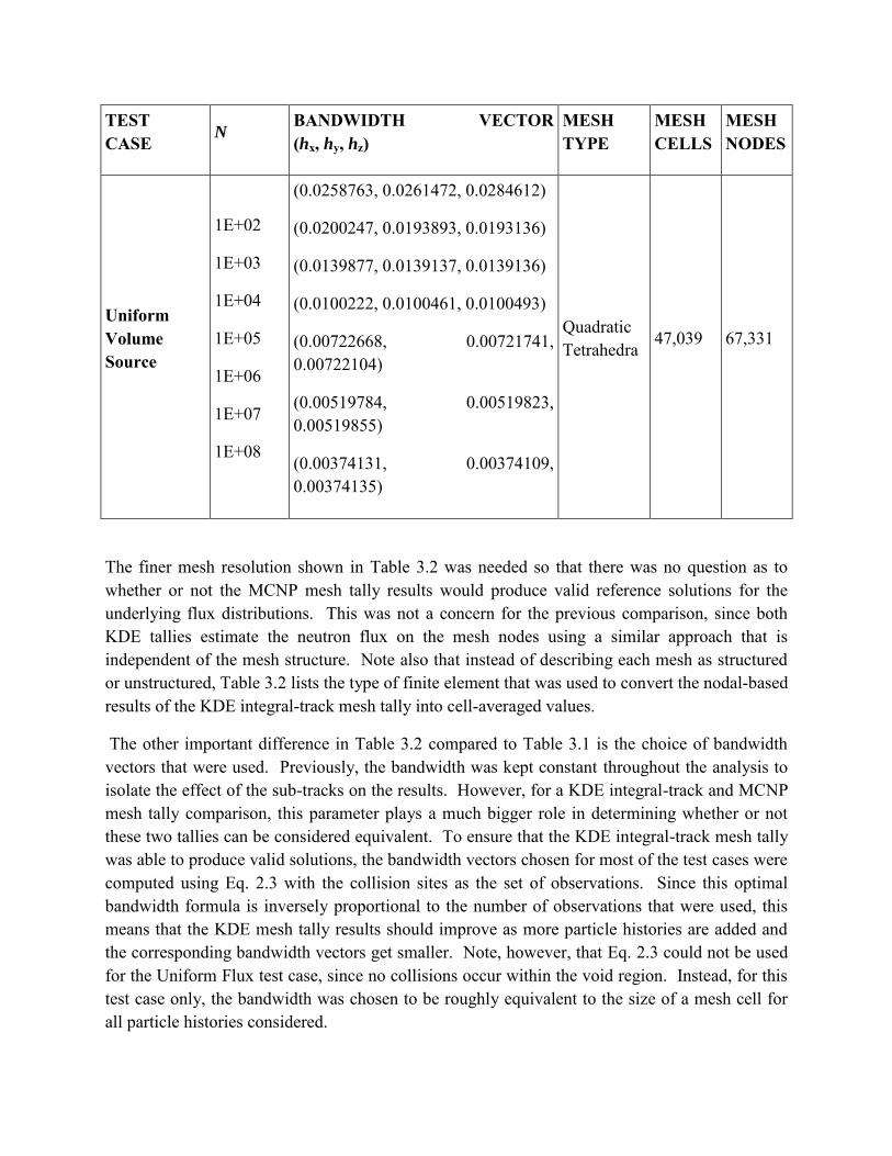
The finer mesh resolution shown in Table 3.2 was needed so that there was no question as to whether or not the MCNP mesh tally results would produce valid reference solutions for the underlying flux distributions. This was not a concern for the previous comparison, since both KDE tallies estimate the neutron flux on the mesh nodes using a similar approach that is independent of the mesh structure. Note also that instead of describing each mesh as structured or unstructured, Table 3.2 lists the type of finite element that was used to convert the nodal-based results of the KDE integral-track mesh tally into cell-averaged values.

The other important difference in Table 3.2 compared to Table 3.1 is the choice of bandwidth vectors that were used. Previously, the bandwidth was kept constant throughout the analysis to isolate the effect of the sub-tracks on the results. However, for a KDE integral-track and MCNP mesh tally comparison, this parameter plays a much bigger role in determining whether or not these two tallies can be considered equivalent. To ensure that the KDE integral-track mesh tally was able to produce valid solutions, the bandwidth vectors chosen for most of the test cases were computed using Eq. 2.3 with the collision sites as the set of observations. Since this optimal bandwidth formula is inversely proportional to the number of observations that were used, this means that the KDE mesh tally results should improve as more particle histories are added and the corresponding bandwidth vectors get smaller. Note, however, that Eq. 2.3 could not be used for the Uniform Flux test case, since no collisions occur within the void region. Instead, for this test case only, the bandwidth was chosen to be roughly equivalent to the size of a mesh cell for all particle histories considered.

Convergence analysis

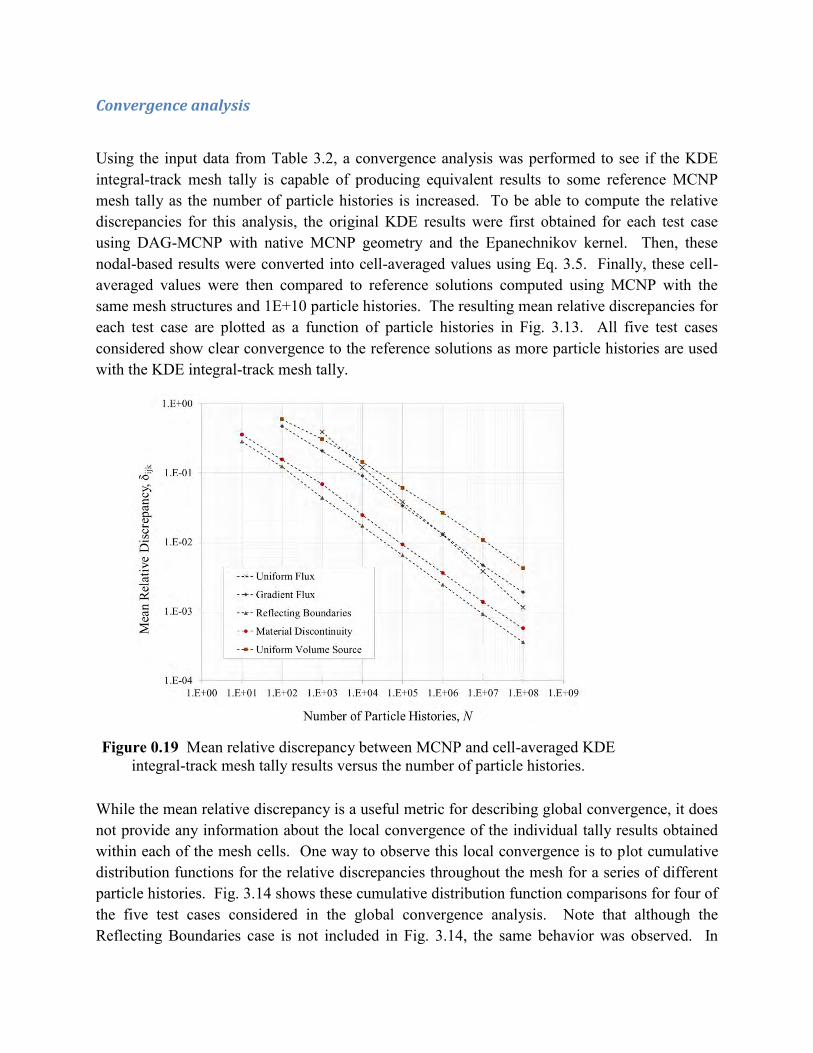
Using the input data from Table 3.2, a convergence analysis was performed to see if the KDE integral-track mesh tally is capable of producing equivalent results to some reference MCNP mesh tally as the number of particle histories is increased. To be able to compute the relative discrepancies for this analysis, the original KDE results were first obtained for each test case using DAG-MCNP with native MCNP geometry and the Epanechnikov kernel. Then, these nodal-based results were converted into cell-averaged values using Eq. 3.5. Finally, these cell-averaged values were then compared to reference solutions computed using MCNP with the same mesh structures and 1E+10 particle histories. The resulting mean relative discrepancies for each test case are plotted as a function of particle histories in Fig. 3.13. All five test cases considered show clear convergence to the reference solutions as more particle histories are used with the KDE integral-track mesh tally.

While the mean relative discrepancy is a useful metric for describing global convergence, it does not provide any information about the local convergence of the individual tally results obtained within each of the mesh cells. One way to observe this local convergence is to plot cumulative distribution functions for the relative discrepancies throughout the mesh for a series of different particle histories. Fig. 3.14 shows these cumulative distribution function comparisons for four of the five test cases considered in the global convergence analysis. Note that although the Reflecting Boundaries case is not included in Fig. 3.14, the same behavior was observed. In

Figure 0.19 Mean relative discrepancy between MCNP and cell-averaged KDE integral-track mesh tally results versus the number of particle histories.

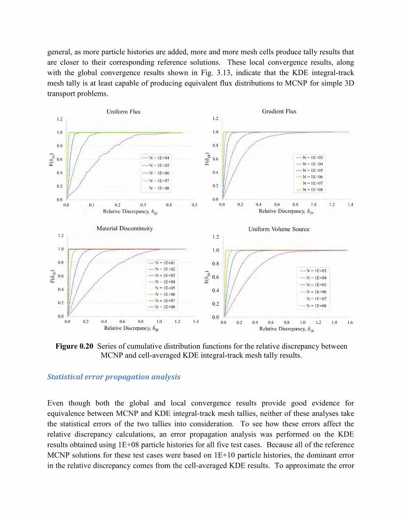
general, as more particle histories are added, more and more mesh cells produce tally results that are closer to their corresponding reference solutions. These local convergence results, along with the global convergence results shown in Fig. 3.13, indicate that the KDE integral-track mesh tally is at least capable of producing equivalent flux distributions to MCNP for simple 3D transport problems.

Statistical error propagation analysis

Even though both the global and local convergence results provide good evidence for equivalence between MCNP and KDE integral-track mesh tallies, neither of these analyses take the statistical errors of the two tallies into consideration. To see how these errors affect the relative discrepancy calculations, an error propagation analysis was performed on the KDE results obtained using 1E+08 particle histories for all five test cases. Because all of the reference MCNP solutions for these test cases were based on 1E+10 particle histories, the dominant error in the relative discrepancy comes from the cell-averaged KDE results. To approximate the error

Figure 0.20 Series of cumulative distribution functions for the relative discrepancy between MCNP and cell-averaged KDE integral-track mesh tally results.

in these cell-averaged values, we can start by making the assumption that the original nodal-based results can be treated as independent random variables. If we have n independent random variables x1, x2 … xn with known statistical errors , … , then we can approximate the error for some function f(x1, x2 … xn) by:

(

)

(

)

(

)

(3.6)

Eq. 3.6 can be used to derive an error propagation formula for the node-to-cell conversion function defined by Eq. 3.5. To obtain this formula, we first need to determine the derivatives for the cell-averaged approximation with respect to the neutron flux at the ith mesh node :

.1

ˆˆ

1

ˆ

~

11 1

p

l

li

llp

l

n

k

lkk

i

ll

i

NjwV

NjwV

(3.7)

Then, we can substitute the derivatives defined by Eq. 3.7 for all of the n mesh nodes used to estimate the flux for a single mesh cell into Eq. 3.6:

,ˆ

),,(~

1

2

1

ˆ

1

2ˆ

2

2),,(~

n

i

p

l

li

llin

i i

zyx NjwV

zyxi

(3.8)

where is the standard deviation obtained using Eq. 2.16 as part of the Monte Carlo simulation for the ith mesh node. Now that the statistical error can be approximated for the cell-averaged result of a single mesh cell (i, j, k) using Eq. 3.8, we can finally determine how this error propagates to the relative discrepancy. Assuming that the cell-averaged KDE and MCNP results are both independent random variables, Eq. 3.6 can be used once again to derive an error propagation formula for the relative discrepancy calculation defined by Eq. 3.1:

(

)

(

)

(

)

(

)

(3.9)

Since the neutron flux for any mesh node or cell that is obtained using Monte Carlo methods is expected to be normally distributed, then the relative discrepancy between the MCNP and KDE results should also be normally distributed. This means that there should be about 68%, 95% and 99.7% of mesh cells with relative discrepancies less than one, two and three standard deviations respectively. Table 3.3 shows the percentage of mesh cells for each test case that had relative discrepancies less than their statistical errors, which were approximated using Eq. 3.9. For four out of the five test cases considered, these results seem to fall short of a normal distribution. Only the Reflecting Boundaries test case produced results that were even close because of the large number of collisions that were used in the approximation. One reason for this difference could be because the nodal-based results were treated as independent random variables for

deriving the error propagation formula defined by Eq. 3.8. Making this assumption can underestimate the statistical error, since the covariance terms for each of the mesh nodes involved in the computation were omitted. If we included these covariance terms, then we should be able to conclude that the relative discrepancy between MCNP and KDE results does in fact fall within statistical expectations. Another way to support this hypothesis is to consider the Uniform Flux test case. Table 3.4 shows the percentage of mesh cells with relative discrepancies less than their statistical error for both MCNP and KDE results when compared directly to the exact solution. Note that the cell-averaged MCNP and nodal-based KDE results both fall approximately within statistical expectations. It is only when the KDE results are converted into their cell-averaged equivalents do we get results that are inconsistent with a normal distribution.

Table 0.3 Distribution of relative discrepancies based on a comparison between KDE (1E+08) and MCNP (1E+10) mesh tally results

TEST CASE % MESH CELLS WITHIN STATISTICAL ERROR

δijk < 1σ δijk < 2σ δijk < 3σ

Uniform Flux 52.8% 88.9% 96.5%

Gradient Flux 50.8% 84.3% 96.5%

Reflecting Boundaries 61.6% 92.6% 99.3%

Material Discontinuity

59.3% 88.4% 97.3%

Uniform Volume Source

52.2% 84.2% 96.6%

Table 0.4 Distribution of relative discrepancies based on a comparison to the exact solution for the Uniform Flux test case

MESH TALLY % MESH CELLS WITHIN STATISTICAL ERROR

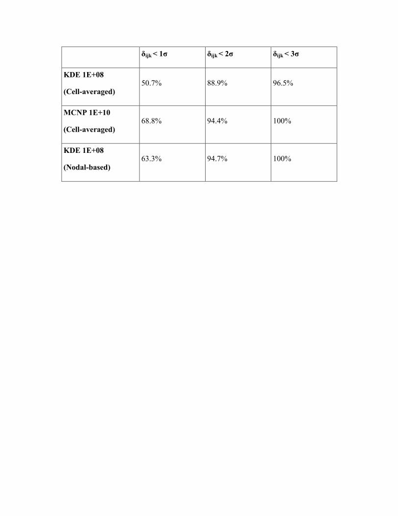
δijk < 1σ δijk < 2σ δijk < 3σ

KDE 1E+08

(Cell-averaged) 50.7% 88.9% 96.5%

MCNP 1E+10

(Cell-averaged) 68.8% 94.4% 100%

KDE 1E+08

(Nodal-based) 63.3% 94.7% 100%

BANDWIDTH SENSITIVITY Selection of an appropriate bandwidth value is essential for obtaining good results from any application that uses KDE methods. This is especially true for KDE-based neutron flux tallies that could be used for the purposes of making critical design decisions on the amount of radiation shielding that is needed for some new nuclear technology. If the neutron flux is underestimated due to a bad bandwidth choice, this could pose a risk to workers as a result of insufficient shielding. On the other hand, if the neutron flux is overestimated this could increase the cost of the design due to adding more shielding than was necessary. As a first step in gaining a better understanding of how this parameter affects the resulting neutron flux, a bandwidth sensitivity experiment was performed using the KDE integral-track mesh tally implemented within DAG-MCNP. This chapter first describes the procedure that was used to perform this experiment in Section 4.1. Then, in Section 4.2 we present the results of the experiment through four different analyses. Finally, Section 4.3 discusses how to choose an effective bandwidth.

Experimental Procedure

The test case used in the bandwidth sensitivity experiment was a slightly larger version of the Uniform Volume Source problem described in Section 3.2, which had angular symmetry and few scattering events to keep things simple. Increasing the outer radius of the sphere from 0.12 cm to 0.14 cm was necessary so that the experiment could be performed with a reasonable range of bandwidth values, without having to worry about implementing a boundary correction technique. Once the geometry was set up in the input file, an unstructured spherical mesh was created with a radius of 0.10 cm and 1010 tetrahedral cells. Then, KDE integral-track mesh tallies based on the Epanechnikov kernel were defined for a series of 20 different bandwidths (ranging from 0.001 to 0.020). Note that because of the angular symmetry in the problem, all three components of the bandwidth were set to the same values for each input file. DAG-MCNP was then run 200 times per bandwidth, using 1E+06 particle histories and a fixed set of 200 random seed numbers. This was done to obtain an estimate for the expected value and sample variance of the kernel density estimated fluxes at each mesh node. When this first stage of the experiment was complete, the entire procedure was repeated using the Uniform kernel to see if the choice of kernel function had any impact on the results as a function of bandwidth. Note that the Uniform kernel was chosen because it has one of the lowest efficiency ratings compared the Epanechnikov kernel [5]. This means that any discrepancy that occurs in the results due to using different kernels would be at a maximum.

After all of the KDE integral-track mesh tally results had been obtained for both the Epanechnikov and Uniform kernels, a finer mesh was created with 26,124 tetrahedral cells to provide a more detailed reference solution. This reference solution was computed using a tetrahedral version of the conventional MCNP mesh tally, with 1E+08 particle histories and the same set of 200 random seed numbers that was used with the KDE integral-track mesh tally. While the MCNP mesh tally produces cell-averaged results in three dimensions, it was still

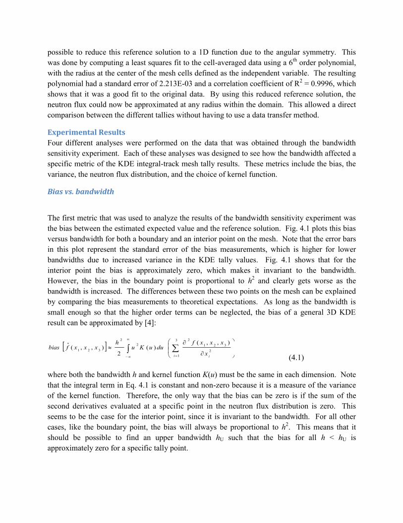
possible to reduce this reference solution to a 1D function due to the angular symmetry. This was done by computing a least squares fit to the cell-averaged data using a 6th order polynomial, with the radius at the center of the mesh cells defined as the independent variable. The resulting polynomial had a standard error of 2.213E-03 and a correlation coefficient of R2 = 0.9996, which shows that it was a good fit to the original data. By using this reduced reference solution, the neutron flux could now be approximated at any radius within the domain. This allowed a direct comparison between the different tallies without having to use a data transfer method.

Experimental Results

Four different analyses were performed on the data that was obtained through the bandwidth sensitivity experiment. Each of these analyses was designed to see how the bandwidth affected a specific metric of the KDE integral-track mesh tally results. These metrics include the bias, the variance, the neutron flux distribution, and the choice of kernel function.

Bias vs. bandwidth

The first metric that was used to analyze the results of the bandwidth sensitivity experiment was the bias between the estimated expected value and the reference solution. Fig. 4.1 plots this bias versus bandwidth for both a boundary and an interior point on the mesh. Note that the error bars in this plot represent the standard error of the bias measurements, which is higher for lower bandwidths due to increased variance in the KDE tally values. Fig. 4.1 shows that for the interior point the bias is approximately zero, which makes it invariant to the bandwidth. However, the bias in the boundary point is proportional to h2 and clearly gets worse as the bandwidth is increased. The differences between these two points on the mesh can be explained by comparing the bias measurements to theoretical expectations. As long as the bandwidth is small enough so that the higher order terms can be neglected, the bias of a general 3D KDE result can be approximated by [4]:

3

12

3212

22

321

),,()(

2),,(ˆ

i ix

xxxfduuKu

hxxxfbias

(4.1)

where both the bandwidth h and kernel function K(u) must be the same in each dimension. Note that the integral term in Eq. 4.1 is constant and non-zero because it is a measure of the variance of the kernel function. Therefore, the only way that the bias can be zero is if the sum of the second derivatives evaluated at a specific point in the neutron flux distribution is zero. This seems to be the case for the interior point, since it is invariant to the bandwidth. For all other cases, like the boundary point, the bias will always be proportional to h2. This means that it should be possible to find an upper bandwidth hU such that the bias for all h < hU is approximately zero for a specific tally point.

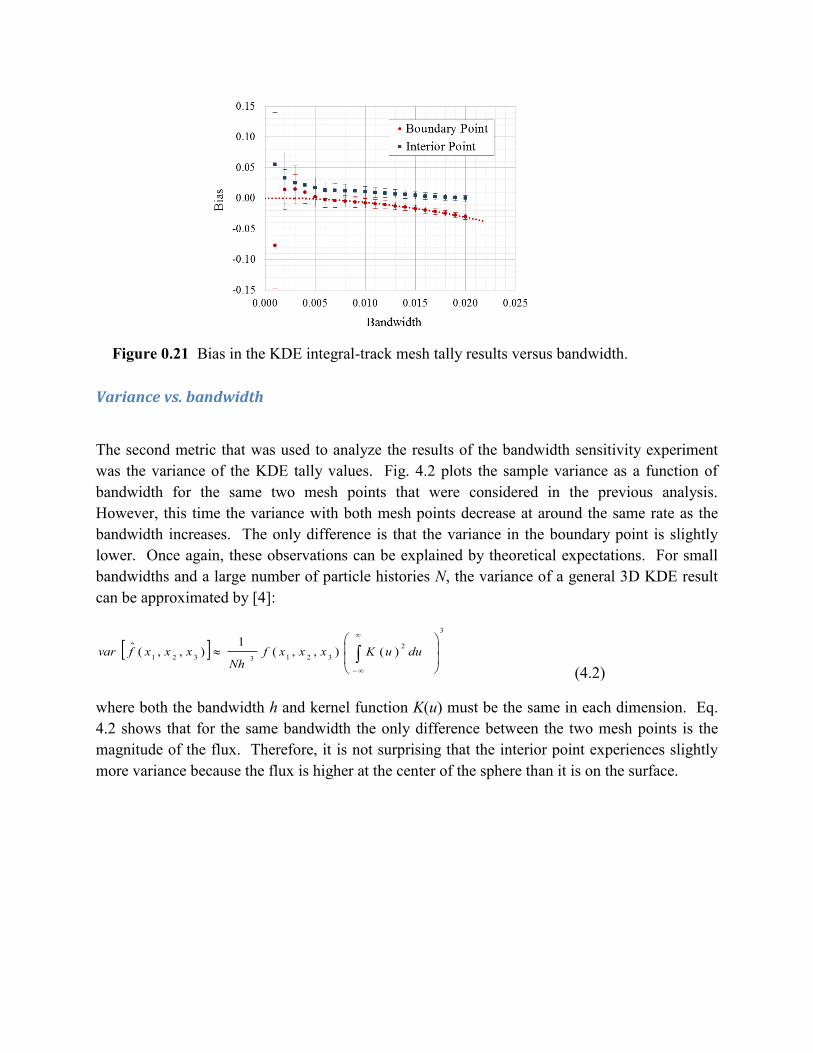
Variance vs. bandwidth

The second metric that was used to analyze the results of the bandwidth sensitivity experiment was the variance of the KDE tally values. Fig. 4.2 plots the sample variance as a function of bandwidth for the same two mesh points that were considered in the previous analysis. However, this time the variance with both mesh points decrease at around the same rate as the bandwidth increases. The only difference is that the variance in the boundary point is slightly lower. Once again, these observations can be explained by theoretical expectations. For small bandwidths and a large number of particle histories N, the variance of a general 3D KDE result can be approximated by [4]:

3

23213321 )(),,(

1),,(ˆ

duuKxxxfNh

xxxfvar

(4.2)

where both the bandwidth h and kernel function K(u) must be the same in each dimension. Eq. 4.2 shows that for the same bandwidth the only difference between the two mesh points is the magnitude of the flux. Therefore, it is not surprising that the interior point experiences slightly more variance because the flux is higher at the center of the sphere than it is on the surface.

Figure 0.21 Bias in the KDE integral-track mesh tally results versus bandwidth.

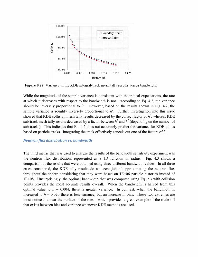
While the magnitude of the sample variance is consistent with theoretical expectations, the rate at which it decreases with respect to the bandwidth is not. According to Eq. 4.2, the variance should be inversely proportional to h3. However, based on the results shown in Fig. 4.2, the sample variance is roughly inversely proportional to h2. Further investigation into this issue showed that KDE collision mesh tally results decreased by the correct factor of h3, whereas KDE sub-track mesh tally results decreased by a factor between h3 and h2 (depending on the number of sub-tracks). This indicates that Eq. 4.2 does not accurately predict the variance for KDE tallies based on particle tracks. Integrating the track effectively cancels out one of the factors of h.

Neutron flux distribution vs. bandwidth

The third metric that was used to analyze the results of the bandwidth sensitivity experiment was the neutron flux distribution, represented as a 1D function of radius. Fig. 4.3 shows a comparison of the results that were obtained using three different bandwidth values. In all three cases considered, the KDE tally results do a decent job of approximating the neutron flux throughout the sphere considering that they were based on 1E+06 particle histories instead of 1E+08. Unsurprisingly, the optimal bandwidth that was computed using Eq. 2.3 with collision points provides the most accurate results overall. When the bandwidth is halved from this optimal value to h = 0.004, there is greater variance. In contrast, when the bandwidth is increased to h = 0.020 there is less variance, but an increase in bias. These two extremes are most noticeable near the surface of the mesh, which provides a great example of the trade-off that exists between bias and variance whenever KDE methods are used.

Figure 0.22 Variance in the KDE integral-track mesh tally results versus bandwidth.

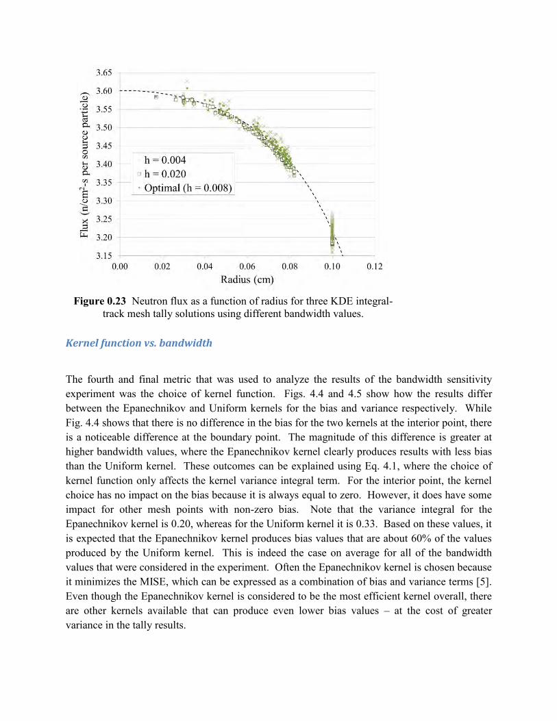
Kernel function vs. bandwidth

The fourth and final metric that was used to analyze the results of the bandwidth sensitivity experiment was the choice of kernel function. Figs. 4.4 and 4.5 show how the results differ between the Epanechnikov and Uniform kernels for the bias and variance respectively. While Fig. 4.4 shows that there is no difference in the bias for the two kernels at the interior point, there is a noticeable difference at the boundary point. The magnitude of this difference is greater at higher bandwidth values, where the Epanechnikov kernel clearly produces results with less bias than the Uniform kernel. These outcomes can be explained using Eq. 4.1, where the choice of kernel function only affects the kernel variance integral term. For the interior point, the kernel choice has no impact on the bias because it is always equal to zero. However, it does have some impact for other mesh points with non-zero bias. Note that the variance integral for the Epanechnikov kernel is 0.20, whereas for the Uniform kernel it is 0.33. Based on these values, it is expected that the Epanechnikov kernel produces bias values that are about 60% of the values produced by the Uniform kernel. This is indeed the case on average for all of the bandwidth values that were considered in the experiment. Often the Epanechnikov kernel is chosen because it minimizes the MISE, which can be expressed as a combination of bias and variance terms [5]. Even though the Epanechnikov kernel is considered to be the most efficient kernel overall, there are other kernels available that can produce even lower bias values – at the cost of greater variance in the tally results.

Figure 0.23 Neutron flux as a function of radius for three KDE integral-track mesh tally solutions using different bandwidth values.

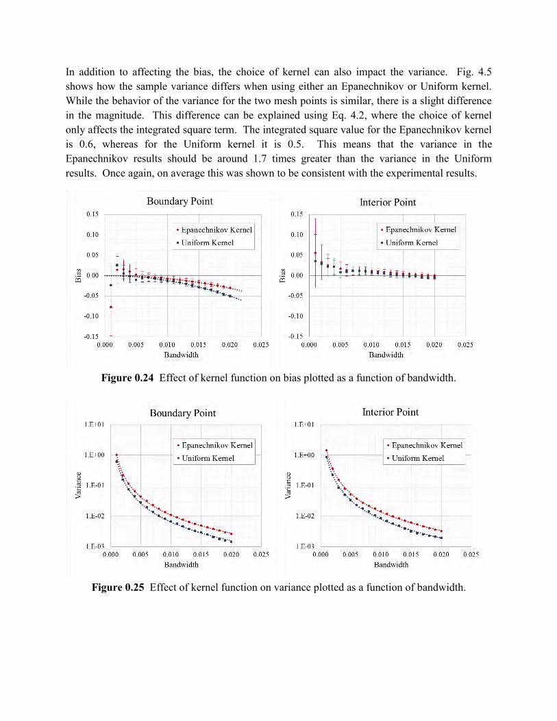
In addition to affecting the bias, the choice of kernel can also impact the variance. Fig. 4.5 shows how the sample variance differs when using either an Epanechnikov or Uniform kernel. While the behavior of the variance for the two mesh points is similar, there is a slight difference in the magnitude. This difference can be explained using Eq. 4.2, where the choice of kernel only affects the integrated square term. The integrated square value for the Epanechnikov kernel is 0.6, whereas for the Uniform kernel it is 0.5. This means that the variance in the Epanechnikov results should be around 1.7 times greater than the variance in the Uniform results. Once again, on average this was shown to be consistent with the experimental results.

Figure 0.24 Effect of kernel function on bias plotted as a function of bandwidth.

Figure 0.25 Effect of kernel function on variance plotted as a function of bandwidth.

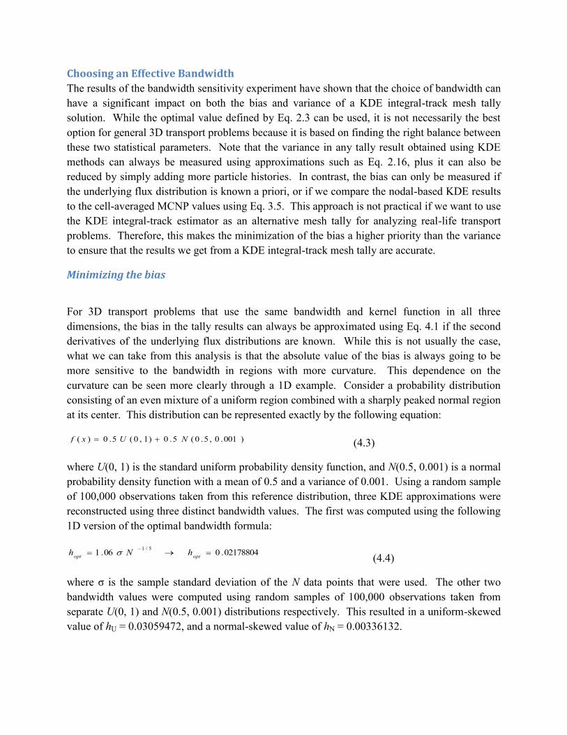
Choosing an Effective Bandwidth

The results of the bandwidth sensitivity experiment have shown that the choice of bandwidth can have a significant impact on both the bias and variance of a KDE integral-track mesh tally solution. While the optimal value defined by Eq. 2.3 can be used, it is not necessarily the best option for general 3D transport problems because it is based on finding the right balance between these two statistical parameters. Note that the variance in any tally result obtained using KDE methods can always be measured using approximations such as Eq. 2.16, plus it can also be reduced by simply adding more particle histories. In contrast, the bias can only be measured if the underlying flux distribution is known a priori, or if we compare the nodal-based KDE results to the cell-averaged MCNP values using Eq. 3.5. This approach is not practical if we want to use the KDE integral-track estimator as an alternative mesh tally for analyzing real-life transport problems. Therefore, this makes the minimization of the bias a higher priority than the variance to ensure that the results we get from a KDE integral-track mesh tally are accurate.

Minimizing the bias

For 3D transport problems that use the same bandwidth and kernel function in all three dimensions, the bias in the tally results can always be approximated using Eq. 4.1 if the second derivatives of the underlying flux distributions are known. While this is not usually the case, what we can take from this analysis is that the absolute value of the bias is always going to be more sensitive to the bandwidth in regions with more curvature. This dependence on the curvature can be seen more clearly through a 1D example. Consider a probability distribution consisting of an even mixture of a uniform region combined with a sharply peaked normal region at its center. This distribution can be represented exactly by the following equation:

)001.0,5.0(5.0)1,0(5.0)( NUxf (4.3)

where U(0, 1) is the standard uniform probability density function, and N(0.5, 0.001) is a normal probability density function with a mean of 0.5 and a variance of 0.001. Using a random sample of 100,000 observations taken from this reference distribution, three KDE approximations were reconstructed using three distinct bandwidth values. The first was computed using the following 1D version of the optimal bandwidth formula:

02178804.006.1 5/1

optopt hNh (4.4)

where σ is the sample standard deviation of the N data points that were used. The other two bandwidth values were computed using random samples of 100,000 observations taken from separate U(0, 1) and N(0.5, 0.001) distributions respectively. This resulted in a uniform-skewed value of hU = 0.03059472, and a normal-skewed value of hN = 0.00336132.

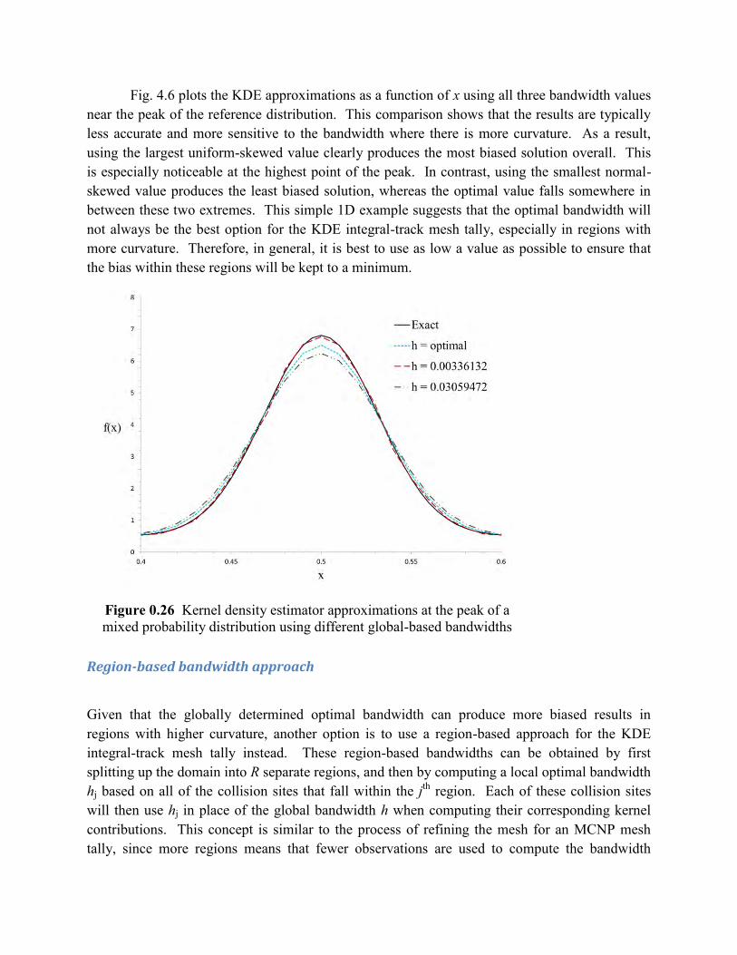
Fig. 4.6 plots the KDE approximations as a function of x using all three bandwidth values near the peak of the reference distribution. This comparison shows that the results are typically less accurate and more sensitive to the bandwidth where there is more curvature. As a result, using the largest uniform-skewed value clearly produces the most biased solution overall. This is especially noticeable at the highest point of the peak. In contrast, using the smallest normal-skewed value produces the least biased solution, whereas the optimal value falls somewhere in between these two extremes. This simple 1D example suggests that the optimal bandwidth will not always be the best option for the KDE integral-track mesh tally, especially in regions with more curvature. Therefore, in general, it is best to use as low a value as possible to ensure that the bias within these regions will be kept to a minimum.

Region-based bandwidth approach

Given that the globally determined optimal bandwidth can produce more biased results in regions with higher curvature, another option is to use a region-based approach for the KDE integral-track mesh tally instead. These region-based bandwidths can be obtained by first splitting up the domain into R separate regions, and then by computing a local optimal bandwidth hj based on all of the collision sites that fall within the jth region. Each of these collision sites will then use hj in place of the global bandwidth h when computing their corresponding kernel contributions. This concept is similar to the process of refining the mesh for an MCNP mesh tally, since more regions means that fewer observations are used to compute the bandwidth

Figure 0.26 Kernel density estimator approximations at the peak of a mixed probability distribution using different global-based bandwidths

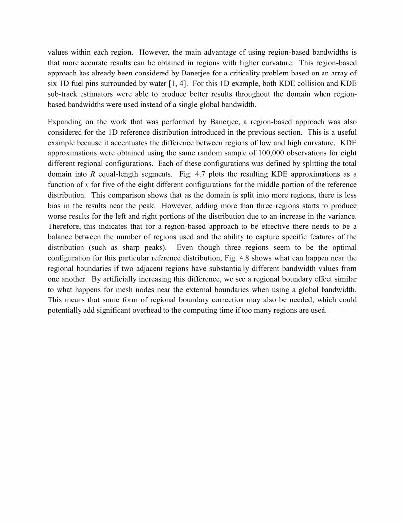
values within each region. However, the main advantage of using region-based bandwidths is that more accurate results can be obtained in regions with higher curvature. This region-based approach has already been considered by Banerjee for a criticality problem based on an array of six 1D fuel pins surrounded by water [1, 4]. For this 1D example, both KDE collision and KDE sub-track estimators were able to produce better results throughout the domain when region-based bandwidths were used instead of a single global bandwidth.

Expanding on the work that was performed by Banerjee, a region-based approach was also considered for the 1D reference distribution introduced in the previous section. This is a useful example because it accentuates the difference between regions of low and high curvature. KDE approximations were obtained using the same random sample of 100,000 observations for eight different regional configurations. Each of these configurations was defined by splitting the total domain into R equal-length segments. Fig. 4.7 plots the resulting KDE approximations as a function of x for five of the eight different configurations for the middle portion of the reference distribution. This comparison shows that as the domain is split into more regions, there is less bias in the results near the peak. However, adding more than three regions starts to produce worse results for the left and right portions of the distribution due to an increase in the variance. Therefore, this indicates that for a region-based approach to be effective there needs to be a balance between the number of regions used and the ability to capture specific features of the distribution (such as sharp peaks). Even though three regions seem to be the optimal configuration for this particular reference distribution, Fig. 4.8 shows what can happen near the regional boundaries if two adjacent regions have substantially different bandwidth values from one another. By artificially increasing this difference, we see a regional boundary effect similar to what happens for mesh nodes near the external boundaries when using a global bandwidth. This means that some form of regional boundary correction may also be needed, which could potentially add significant overhead to the computing time if too many regions are used.

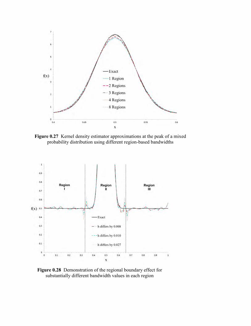
Figure 0.27 Kernel density estimator approximations at the peak of a mixed probability distribution using different region-based bandwidths

Figure 0.28 Demonstration of the regional boundary effect for substantially different bandwidth values in each region

SUMMARY AND FUTURE WORK This concluding chapter first discusses how the KDE approach can be applied to mesh tallies as part of a production Monte Carlo transport code in Section 5.1. Then, in Section 5.2 we summarize the results of two detailed quantitative comparisons that were performed on this new KDE mesh tally based on integrated particle tracks for verification purposes. Section 5.3 highlights the important points that were discovered by performing a sensitivity analysis on the choice of bandwidth that is used to obtain the KDE integral-track mesh tally results. Finally, in Section 5.4 we present a general summary and introduce some key areas where more research is needed before mesh tallies based on a KDE approach can be considered a viable alternative to conventional mesh tallies for real-life applications.

Kernel Density Estimated Monte Carlo Mesh Tallies

The 3D kernel density estimator was introduced in Chapter 2 as a non-parametric method that can be used to reconstruct the shape of a neutron flux distribution using Monte Carlo methods. This estimator had been used previously to derive KDE versions of conventional collision and track length estimators that are both capable of estimating the flux at any point within some geometric domain. While these two estimators could easily be implemented as mesh tallies, the accuracy of their contributions is dependent on either the collision or pseudo-collision density. Even though the pseudo-collision density used with the original KDE track estimator could always be increased by adding more sub-tracks, this approach could end up becoming quite expensive computationally for general transport problems. Therefore, as an alternative it was suggested that a better approach was to consider a new KDE track length estimator based on integrated particle tracks instead of pseudo-collisions.

The KDE integral-track estimator was formally derived from its predecessor by first redefining the pseudo-collision points in terms of a common path length integral. Then, these new definitions were substituted into the KDE sub-track estimator and the final result was obtained by taking the limit as the number of sub-tracks approached infinity. This final form of the KDE integral-track estimator was then implemented within DAG-MCNP as an alternative mesh tally, using the set of mesh nodes as the calculation points for which the neutron flux was to be evaluated. Since typical input meshes can have thousands of nodes, for efficiency purposes it was essential to determine which of these calculation points would be evaluated with each track segment that was tallied. This subset of calculation points was designated the neighborhood region, which consists of all of the mesh nodes expected to add non-trivial contributions to the tally.

Once the set of mesh nodes within the neighborhood region has been determined for each track segment, the next step in the KDE integral-track mesh tally implementation is to compute the new computations that will be added. This is done by integrating the kernel function with respect to the path length along the track using a 4-point Gaussian quadrature method. Note that a numerical integration technique was used because it computed the exact integral based on the

Epanechnikov kernel using fewer operations than the analytical solution. As a part of this integration process, each mesh node that is to be evaluated is first checked for valid integration limits. These limits are obtained by constructing intervals for the range of path lengths that result in non-zero kernel contributions, and then comparing them to the total track length. Then, only the mesh nodes with valid integration limits are actually evaluated for every track segment that is tallied using the KDE integral-track estimator.

Quantitative Mesh Tally Comparisons

The primary focus of Chapter 3 was to perform a quantitative comparison on the KDE integral-track mesh tally that was implemented within DAG-MCNP to show that it is capable of producing equivalent results to other mesh tally implementations. A series of five verification test cases were proposed, with each case representing a particular feature that commonly occurs in general Monte Carlo transport problems. All five of these test cases were first used to quantitatively compare KDE integral-track and KDE sub-track mesh tally results, which was simple to do since both tallies approximate the neutron flux directly on the mesh nodes. Using the mean relative discrepancy as the error metric, it was shown that both the tally means and variances computed by the KDE sub-track mesh tally converge on average to the results of the KDE integral-track mesh tally as the number of sub-tracks is increased. In addition to producing more accurate results, the KDE integral-track estimator was also able to calculate those results in the same amount of time as its predecessor using only two sub-tracks.

While computing the relative discrepancy between the two KDE mesh tallies was straightforward, this was not the case for a quantitative comparison performed between the KDE integral-track and MCNP mesh tallies. Since both of these tallies evaluate their contributions differently, a data transfer method was needed to first convert the nodal-based KDE results into equivalent cell-averaged values before any calculations could be made. This conversion was done for all five test cases using finite element theory to interpolate the known flux results at the mesh nodes of a 3D finite mesh element to a series of cubature points, which could then be used in a Gaussian cubature rule to approximate the cell-averaged values. However, even though this node-to-cell data transfer method was shown to be more effective than a basic cell-to-node approach, it was also shown that any comparison between nodal-based and cell-averaged values also depends on how well MCNP resolves the underlying flux distribution. Therefore, for the purposes of quantitatively comparing KDE integral-track and MCNP mesh tally results, finer mesh resolutions were used to ensure that MCNP would produce valid reference solutions. The final outcome of both this comparison and the previous one was that the KDE integral-track mesh tally is indeed capable of producing equivalent results to other mesh tally implementations for simple 3D transport problems.

Bandwidth Sensitivity

Even though the results from the KDE integral-track mesh tally were shown to be comparable to both the KDE sub-track and MCNP mesh tallies in Chapter 3, before we can even consider using this alternative with more complicated test cases we need to obtain a better understanding of the bandwidth. Therefore, as a first step, the choice of this parameter was discussed in detail in Chapter 4 through the analysis of a bandwidth sensitivity experiment that was performed using the KDE integral-track mesh tally. This analysis considered how the bandwidth affects the bias, the variance, the neutron flux distribution, and the choice of kernel function for a test case with angular symmetry and few scattering events to keep things simple. Note that because of the angular symmetry in the problem, it was possible to reduce the 3D neutron flux distribution into an equivalent 1D reference solution so that no boundary correction technique was needed to compare the final results.

The effect of the bandwidth on the bias in the experimental results was found to be dependent on the curvature of the underlying flux distribution. For regions where there is no curvature, the bias will always be zero and is therefore invariant to the choice of bandwidth. In regions with non-zero curvature, however, the bias is proportional to h2 when the same value is used in all three dimensions. Whereas the behavior of the bias was shown to be dependent on curvature, in general as the bandwidth was increased the variance always decreased. Unfortunately, this means that improving the variance by increasing the bandwidth also increases the bias for regions with non-zero curvature. This trade-off as a function of bandwidth was most noticeable in the results for the neutron flux distribution near the surface of the mesh, which indicates that this is a bigger issue in regions with higher curvature. In addition to considering both the bias and variance, the effect of the bandwidth was also observed for two different kernel functions. While the behavior of these two statistical parameters with respect to bandwidth was the same for both the Epanechnikov and Uniform kernels, there was a slight discrepancy between their respective magnitudes. However, this discrepancy was shown to be consistent with theoretical expectations and is negligible for lower bandwidth values.

Since the magnitude of the variance can be approximated as part of a Monte Carlo simulation, and can always be reduced by using more particle histories, the bandwidth that is used with the KDE integral-track mesh tally should always be chosen with the primary goal of minimizing the bias. A known 1D probability distribution was used as an example to show that using a globally determined optimal bandwidth is not always the best choice, especially in regions with more curvature. In general, it is best to use as low a value as possible for the bandwidth to ensure that the bias within these regions will be kept to a minimum. As an alternative for improving the accuracy of the KDE integral-track mesh tally, another option is to use region-based bandwidths instead of the global bandwidth approach. However, while this can reduce the bias in regions with higher curvature, it can still potentially cause issues for mesh nodes near the regional boundaries. Therefore, if this region-based bandwidth approach is to be useful, it may be necessary to implement a regional boundary correction to get valid results.

Future Work

Through the work that was presented in this paper, we have shown that a mesh tally based on the KDE integral-track estimator is a promising alternative to other mesh tally implementations for a few reasons. First, it produces more accurate results than the original KDE track length estimator because it uses full particle tracks instead of relying on pseudo-collisions. This improved accuracy also comes with no penalty to the overall execution time. Second, it is capable of producing better results than MCNP for transport problems with strong gradients defined on coarser meshes because it approximates the neutron flux at the mesh nodes instead of computing cell-averaged values. Finally, it can be used with either structured or unstructured meshes that consist of any combination of different mesh cells because it computes its contributions independent of the mesh structure. This enables the KDE integral-track estimator to be applicable to a wide variety of general 3D transport problems.

Although the KDE integral-track mesh tally is capable of producing comparable results to MCNP for simple transport problems, there is still more work to be done before it can truly be considered a viable alternative in production Monte Carlo transport codes. This future work can be classified into two distinct categories: development-based and research-based. For the development-based work, the first stage will be to implement a boundary correction technique so that the larger bias in the results for mesh nodes within one bandwidth of any external boundaries will be eliminated. There are many methods available that will achieve this goal, but to keep things simple we are initially going to focus on the boundary kernel method that was used by Banerjee for the original KDE track length estimator [1, 4].

Once a boundary correction technique has been implemented, the next stage of the development-based work will be to implement KDE integral-track mesh tallies within the Monte Carlo transport code currently being developed at Oak Ridge National Laboratory called SHIFT. An initial implementation of the geometry interface has already been completed and unit tested using the same methods from the DAGMC toolkit that were also used to create DAG-MCNP. Once this geometry interface is fully integrated into the code, the DAG-SHIFT implementation will be available for performing a Monte Carlo transport simulation using SHIFT directly on a CAD-based geometry. One of the end goals of this work is to see if the KDE integral-track estimator is a viable alternative for computing the uncollided neutron flux within SHIFT.

In addition to the more development-based work, there is also plenty of future research-based work to be done. Perhaps the most important is to continue working on obtaining a better understanding of the bandwidth and how it affects the accuracy of the KDE integral-track mesh tally results. We now know that the results are more sensitive to the choice of bandwidth in regions with higher curvature, and that region-based bandwidths can be more accurate than a global bandwidth approach. But what we have not yet explored is all of the other methods that are available for choosing the bandwidth, or if it is even possible to measure the accuracy of our results without needing a reference solution. Since theoretical equations do exist for approximating the bias, perhaps these can be manipulated in some way to provide a validity test

for the bandwidth parameter – much like the relative standard error is a measure of the statistical variance in the results. If this is possible, then this will be a big step towards making the KDE integral-track mesh tally a viable alternative to the MCNP mesh tally for real-life applications.

REFERENCES [1] K. Banerjee and W. R. Martin, “Kernel Density Estimation Method for Monte Carlo Global

Flux Tallies,” Nuclear Science and Engineering, 170, pp.234-250 (2012).

[2] K. Banerjee and W. R. Martin, “Applying the Kernel Density Flux Estimator to Estimate Flux at a Point,” Transactions of the American Nuclear Society, 100, pp.294-296 (2009).

[3] T. Yamamoto, “Non-regionwise Weight Cancellation for Monte Carlo Higher Order Criticality Calculations using Kernel Density Estimator,” Annals of Nuclear Energy, 38, pp.2515-2520 (2011).

[4] K. Banerjee, “Kernel Density Estimator Methods for Monte Carlo Radiation Transport,” Ph.D. Thesis, Nuclear Engineering and Radiological Sciences, University of Michigan (2010).

[5] B. W. Silverman, Density Estimation for Statistics and Data Analysis, Chapman and Hall, London (1986).

[6] T. J. Tautges and P. P. H. Wilson et al., “Acceleration Techniques for Direct Use of CAD-based Geometries in Monte Carlo Radiation Transport,” Proceedings of the International Conference on Mathematics, Computational Methods & Reactor Physics (M&C 2009), Saratoga Springs, New York, May 3-7, 2009, American Nuclear Society (2009).

[7] D. P. Griesheimer, “Functional expansion tallies for Monte Carlo simulations,” Ph.D. Thesis, Nuclear Engineering and Radiological Sciences, University of Michigan (2005).

[8] T. J. R. Hughes, The Finite Element Method: Linear Static and Dynamic Finite Element Analysis, Dover Publications, New York (2000).

Task 3: Implementation in Production Monte Carlo Software The goal for this final task was to add the unstructured mesh tally capability to Shift, a new Monte Carlo reactor physics code from Oak Ridge National Laboratory (ORNL). There is particular interest in the combination of DAGMC geometry with KDE-based tallies as it will allow for replicated geometry, decomposed mesh, and the ability to tally flux moments at points on that mesh. One use case for shift is to generate the first collided source for calculations in its companion discrete ordinates code, Denovo. When using certain discretizations within Denovo, it is necessary to have node-centered values of the flux moments, rather than cell-averaged values common of most tally estimators.

In the final months of this project, we were successful at implementing DAGMC within Shift with units tests to ensure correct implementation. Two main thrusts remain to complete this effort, with plans to do so in FY13, under separate funding.

Follow-up Task A: Extend Shift for replicated domain, decomposed mesh

operation The current development effort for Shift has focused on a fully decomposed domain, often with overlapping regions, to facilitate its primary mission. For the particular application that is driving this task, however, it is preferable to represent the entire geometric domain on each process and only decompose the mesh on which the tallies are being summed, the latter due to memory constraints. This hybrid is particularly useful for first-collided source calculations since there will be no particle interactions and particle histories may stream across large parts of the geometric domain. Under this paradigm, it will be possible to use a combination of deterministic integral transport steps, based on ray-tracing with the DAGMC interface, to bring histories into the mesh sub-domain of interest to a given process, and then use the KDE tally capability within that mesh sub-domain.

Follow-up Task B: Implement KDE estimators for higher order flux moments The method to accomplish KDE tallies will be extended to support higher order flux moments and will be implemented under the appropriate interface to Shift.

The current implementation of the KDE tallies is only appropriate for tallying scalar flux, and not for tallying higher order flux moments. While mathematically straightforward to tally a different basis function, the numerical implementation may introduce some new approximations, particularly in the integration/quadrature along a track length.

Finally, some interface code will be written to allow Shift to invoke the methods at the appropriate time, generally at each track in the transport process.