Advanced Management Accounting Vol. I
791
description
Advanced Management Accounting Vol. I
Transcript of Advanced Management Accounting Vol. I


FINAL (NEW) COURSE STUDY MATERIAL
PAPER 5
Advanced Management Accounting
BOARD OF STUDIES
THE INSTITUTE OF CHARTERED ACCOUNTANTS OF INDIA

This study material has been prepared by the faculty of the Board of Studies. The objective of the study material is to provide teaching material to the students to enable them to obtain knowledge and skills in the subject. Students should also supplement their study by reference to the recommended text books. In case students need any clarifications or have any suggestions to make for further improvement of the material contained herein, they may write to the Director of Studies.
All care has been taken to provide interpretations and discussions in a manner useful for the students. However, the study material has not been specifically discussed by the Council of the Institute or any of its Committees and the views expressed herein may not be taken to necessarily represent the views of the Council or any of its Committees.
Permission of the Institute is essential for reproduction of any portion of this material.
THE INSTITUTE OF CHARTERED ACCOUNTANTS OF INDIA
All rights reserved. No part of this book may be reproduced, stored in retrieval system, or transmitted, in any form, or by any means, Electronic, Mechanical, photocopying, recording, or otherwise, without prior permission in writing from the publisher.
Updated Edition : January, 2011
Website : www.icai.org
Department/ : Board of Studies Committee
E-mail : [email protected]
ISBN No. : 978-81-8441-076-1
Price : `
Published by : The Publication Department on behalf of The Institute of Chartered Accountants of India, ICAI Bhawan, Post Box No. 7100, Indraprastha Marg, New Delhi-110 002, India.
Typeset and designed at Board of Studies.
Printed by : Sahitya Bhawan Publications, Hospital Road, Agra 282 003 January/2011/20,000 Copies (Updated)

A WORD ABOUT STUDY MATERIAL
The Institute of Chartered Accountants of India develops the course curriculum for its students and undertakes the periodic review of the course keeping in mind the developments in different subjects world wide and the objective of equipping the students with necessary knowledge and skill to serve the needs of Indian industry. The change in business process across the globe and the continuous research work have evolved various advanced tools and techniques in the field of management accounting. The Institute has brought the modern techniques like Just in Time ( JIT), Total Quality Management ( TQM), Life Cycle Costing, Value Analysis, Throughput Accounting etc in the syllabus of Advanced Management Accounting. Moreover, Time Series Analysis and Test of Hypothesis have also been brought into the Operation Research portion of the syllabus to equip the students with the research techniques. Equal importance has also been given in traditional tools of management accounting like Standard Costing, Budgeting, CVP Analysis etc which have great role to play in controlling and managing costs as well as decision making. The Board of Studies which is instrumental in imparting theoretical education for the students of Chartered Accountancy Course develops the Study Materials of all subjects with the objective of developing the clear understanding of the concept of different topics covered in the subject among the students. The Study Material on Advanced Management Accounting covers nineteen chapters and topics included in each chapter are explained in details with explanation, examples and illustrations. As Management Accounting builds on various cross functional areas, comprehensive understanding of the subject is possible if only one covers all the topics of management accounting. A real life problem relates a number of topics of management accounting which are closely linked and its solution asks for clear understanding of all related topics. Thus, the students are advised to go though the whole study material and are expected to supplement their studies by referring to the recommended books of the subject in order to equip themselves with necessary professional knowledge of the subject. If required, they are also advised to brush up their knowledge of related topics of IPCC level. The Board of Studies has also developed Practice Manual of the subject to provide an effective guidance material by providing clarification / solution to very important topics / issues, both theoretical and practical, of different chapters. Moreover, it will serve as Revision Help book towards preparing for Final Examination of the Institute and help the students in identifying the gaps in the preparation of the examination and developing plan to make it up. It will also provide standard of solutions to the questions which will act as a bench mark towards developing the skill of students on framing standard answer to a question. For any further clarification/guidance, students are requested to send their queries at [email protected],
Happy Reading and Best Wishes!

SYLLABUS
PAPER 5 : ADVANCED MANAGEMENT ACCOUNTING (One paper – Three hours – 100 marks)
Level of Knowledge: Advanced knowledge Objective: To apply various management accounting techniques to all types of organizations for planning, decision making and control purposes in practical situations. To develop ability to apply quantitative techniques to business problems 1. Cost Management
(a) Developments in the business environment; just in time; manufacturing resources planning; (MRP); automated manufacturing; synchronous manufacturing and back flush systems to reflect the importance of accurate bills of material and routings; world class manufacturing; total quality management.
(b) Activity based approaches to management and cost analysis
(c) Analysis of common costs in manufacturing and service industry
(d) Techniques for profit improvement, cost reduction, and value analysis
(e) Throughput accounting
(f) Target costing; cost ascertainment and pricing of products and services
(g) Life cycle costing
(h Shut down and divestment.
2. Cost Volume Profit Analysis (a) Relevant cost
(b) Product sales pricing and mix
(c) Limiting factors
(d) Multiple scarce resource problems
(e) Decisions about alternatives such as make or buy, selection of products, etc.
3. Pricing Decisions (a) Pricing of a finished product
(b) Theory of price
(c) Pricing policy

(d) Principles of product pricing
(e) New product pricing
(f) Pricing strategies
(g) Pricing of services
(h) Pareto analysis
4. Budgets and Budgetary Control The budget manual, Preparation and monitoring procedures, Budget variances, Flexible budgets, Preparation of functional budget for operating and non-operating functions, Cash budgets, Capital expenditure budget, Master budget, Principal budget factors.
5. Standard Costing and Variance Analysis Types of standards and sources of standard cost information; evolution of standards, continuous -improvement; keeping standards meaningful and relevant; variance analysis; disposal of variances.
(a) Investigation and interpretation of variances and their inter relationship
(b) Behavioural considerations.
6. Transfer pricing (a) Objectives of transfer pricing
(b) Methods of transfer pricing
(c) Conflict between a division and a company
(d) Multi-national transfer pricing.
7. Cost Management in Service Sector
8. Uniform Costing and Inter firm comparison
9. Profitability analysis - Product wise / segment wise / customer wise
10. Financial Decision Modeling
(a) Linear Programming
(b) Network analysis - PERT/CPM, resource allocation and resource leveling
(c) Transportation problems
(d) Assignment problems
(e) Simulation
(f) Learning Curve Theory
(g) Time series forecasting
(h) Sampling and test of hypothesis

ADVANCED MANAGEMENT ACCOUNTING
CONTENTS
CHAPTER 1 – DEVELOPMENTS IN THE BUSINESS ENVIRONMENT
1.1 The impact of changing environment on cost and management accounting ............ 1.1 1.2 Total Quality Management ..................................................................................... 1.3 1.3 Activity Based Cost Management ......................................................................... 1.30 1.4 Target Costing ..................................................................................................... 1.53 1.5 Life Cycle Costing ............................................................................................... 1.70 1.6 Value Chain Analysis ........................................................................................... 1.74 1.7 Cost control and cost reduction .......................................................................... 1.100 1.8 Computer-aided manufacturing .......................................................................... 1.104 1.9 Just in time ........................................................................................................ 1.105 1.10 Manufacturing resources planning (MRP I & II)................................................... 1.115 1.11 Synchronous manufacturing............................................................................... 1.119 1.12 Business Process Re-engineering...................................................................... 1.119 1.13 Throughput accounting ...................................................................................... 1.120 1.14 Shut down & divestment..................................................................................... 1.126
CHAPTER 2 – COST CONCEPTS IN DECISION MAKING
2.1 Introduction ........................................................................................................... 2.1 2.2 Application of incremental/differential cost techniques in managerial decisions....................................................................................... 2.40
CHAPTER 3 – CVP ANALYSIS & DECISION MAKING
3.1 Introduction............................................................................................................ 3.1 3.2 Important factors in marginal costing decisions ...................................................... 3.3 3.3 Pricing decisions under special circumstances ....................................................... 3.4 3.4 Make or buy decision ........................................................................................... 3.14 3.5 Shut down or continue decision............................................................................ 3.26

3.6 Export V/s local sale decision............................................................................... 3.32 3.7 Expand or contract decision ................................................................................. 3.35 3.8 Product mix decision............................................................................................ 3.37 3.9 Price-mix decision................................................................................................ 3.53
CHAPTER 4: PRICING DECISIONS 4.1 Introduction............................................................................................................ 4.1 4.2 Theory of price....................................................................................................... 4.1 4.3 Pricing policy ......................................................................................................... 4.3 4.4 Pricing of finished product...................................................................................... 4.5 4.5 New product pricing ............................................................................................... 4.6 4.6 Pricing of finished product...................................................................................... 4.7 4.7 Pricing strategies ................................................................................................... 4.8 4.8 Pareto analysis .................................................................................................... 4.22
CHAPTER 5 – BUDGET & BUDGETARY CONTROL
5.1 Introduction............................................................................................................ 5.1 5.2 Strategic Planning, Budgetary Planning and Operational Planning ......................... 5.1 5.3 The preparation of budgets .................................................................................... 5.2 5.4 The interrelationship of budgets ........................................................................... 5.12 5.5 Using spreadsheets in budget preparation ........................................................... 5.12 5.6 Preparation of fixed and flexible budgets.............................................................. 5.12 5.7 Zero Base Budgeting ........................................................................................... 5.37 5.8 Performance Budgeting (PB)................................................................................ 5.40 5.9 Budget Ratio........................................................................................................ 5.43 5.10 Budget Variance .................................................................................................. 5.45
CHAPTER 6 – STANDARD COSTING
6.1 Introduction............................................................................................................ 6.1 6.2 Definitions.............................................................................................................. 6.2 6.3 Computation of variances....................................................................................... 6.5

6.4 Reporting of variances ......................................................................................... 6.47 6.5 Accounting procedure for standard cost ............................................................... 6.61 6.6 Behavioural aspects of Standard Costing ............................................................. 6.70
CHAPTER 7 – COSTING OF SERVICE SECTOR 7.1 Introduction ........................................................................................................... 7.1 7.2 Main characteristics of service sector ..................................................................... 7.1 7.3 Collection of costing data in service sector ............................................................. 7.2 7.4 Costing methods used in service sector ................................................................. 7.3 7.5 Pricing by service sector ........................................................................................ 7.7
CHAPTER 8 – TRANSFER PRICING 8.1 Introduction............................................................................................................ 8.1 8.2 Objectives of transfer pricing system...................................................................... 8.1 8.3 Methods of transfer pricing..................................................................................... 8.1 8.4 Conflict between a division and the company ....................................................... 8.27 8.5 Multinational transfer pricing ................................................................................ 8.28
CHAPTER 9: UNIFORM COSTING AND INTER FIRM COMPARISON 9.1 Uniform costing...................................................................................................... 9.1 9.2 Inter-firm comparison ............................................................................................. 9.3
CHAPTER 10 – COST SHEET, PROFITABILITY ANALYSIS AND REPORTING 10.1 Introduction.......................................................................................................... 10.1 10.2 Cost Sheets (Contentious issues) ........................................................................ 10.1 10.3 Profitability statements......................................................................................... 10.4 10.4 The Balanced Scorecard.................................................................................... 10.10
CHAPTER 11 – LINEAR PROGRAMMING 11.1 Introduction.......................................................................................................... 11.1 11.2 Graphical Method ................................................................................................ 11.3 11.3 Trial & Error method of solving Linear Programming Problem............................. 11.17 11.4 The simplex method........................................................................................... 11.20 11.5 Simplex method for minimization problems......................................................... 11.27

11.6 Marginal value of a resource .............................................................................. 11.32 11.7 Some remarks ................................................................................................... 11.33 11.8 Practical applications of linear programming ...................................................... 11.40 11.9 Limitations of linear programming ...................................................................... 11.61
CHAPTER 12 – THE TRANSPORTATION PROBLEM
12.1 Introduction.......................................................................................................... 12.1 12.2 Methods of finding initial solution to transportation problems ................................ 12.3 12.3 Optimality test...................................................................................................... 12.8 12.4 Special cases .................................................................................................... 12.15 12.5 Maximisation transportation problems ................................................................ 12.19 12.6 Prohibited routes................................................................................................ 12.22 12.7 Miscellaneous illustrations ................................................................................. 12.25
CHAPTER 13 – THE ASSIGNMENT PROBLEM
13.1 Introduction.......................................................................................................... 13.1 13.2 The Assignment algorithm.................................................................................... 13.1 13.3 Unbalanced assignment problems........................................................................ 13.7
CHAPTER 14 – CRITICAL PATH ANALYSIS
14.1 Introduction.......................................................................................................... 14.1 14.2 General framework of PERT/CPM........................................................................ 14.2 14.3 Advantages of critical path analysis...................................................................... 14.2 14.4 Fundamentals of a CPA network .......................................................................... 14.3 14.5 Critical path analysis .......................................................................................... 14.19
CHAPTER 15 – PROGRAM EVALUATION AND REVIEW TECHNIQUE
15.1 Introduction.......................................................................................................... 15.1 15.2 Probability of achieving completion date............................................................... 15.2 15.3 A few comments on assumptions of PERT & CPM ............................................. 15.11 15.4 Distinction between PERT & CPM...................................................................... 15.12

15.5 Updating the network ......................................................................................... 15.12 15.6 Project crashing ................................................................................................. 15.14 15.7 Resource smoothing .......................................................................................... 15.25 15.8 Resource levelling ............................................................................................. 15.29 15.9 Miscellaneous illustrations ................................................................................. 15.29
CHAPTER 16 – SIMULATION
16.1 Introduction.......................................................................................................... 16.1 16.2 What is simulation?.............................................................................................. 16.1 16.3 Monte Carlo simulation ........................................................................................ 16.2 16.4 Simulation and inventory control ........................................................................ 16.14 16.5 Miscellaneous illustrations ................................................................................. 16.17 16.6 Random numbers table ...................................................................................... 16.25
CHAPTER 17 – LEARNING CURVE THEORY
17.1 Introduction.......................................................................................................... 17.1 17.2 Distinctive features of learning curve theory in manufacturing environment........... 17.2 17.3 The learning curve ratio ....................................................................................... 17.2 17.4 Learning curve equation....................................................................................... 17.3 17.5 Learning curve application ................................................................................... 17.4 17.6 Limitations of learning curve theory ...................................................................... 17.6
CHAPTER 18 – TESTING OF HYPOTHESIS
18.1 Introduction.......................................................................................................... 18.1 18.2 Concept of hypothesis.......................................................................................... 18.1 18.3 Tails of a test ....................................................................................................... 18.2 18.4 Procedure in Hypothesis testing........................................................................... 18.3 18.5 Hypothesis testing for population mean................................................................ 18.4 18.6 Hypothesis test concerning proportion.................................................................. 18.7
18.7 Test for equality of two means (Large samples) (n1+n2−2 30) ............................. 18.11 18.8 Test for equality of proportion............................................................................. 18.15

18.9 Chi Square Distribution (X2 distribution) ............................................................. 18.16 18.10 Tests of hypothesis about the variance of two populations ................................. 18.21 18.11 Analysis of Variance-A test for homogeneity of Mean ......................................... 18.23 18.12 Analysis of variance in manifold classification .................................................... 18.27
CHAPTER 19 – TIME SERIES ANALYSIS & FORECASTING
19.1 Introduction.......................................................................................................... 19.1 19.2 Importance of time series analysis ....................................................................... 19.1 19.3 Components of a time series................................................................................ 19.2 19.4 Smoothing methods in time series...................................................................... 19.18 19.5 Existence of trend .............................................................................................. 19.23 19.6 Forecasting using time series............................................................................. 19.25

1 Developments in the Business Environment
LEARNING OBJECTIVES : After studying this unit you will be able to : • Understand the impact of changing environment on cost and management accounting • Know the six C’s of Total Quality Management • Appreciate the Meaning, Purpose and benefit of Activity based costing • Discuss the Activity based Management model • Understand the Main features of Target costing system • Ascertain the cost accountants role in Target Costing environment • Differentiate between the various phases of product life cycle • Understand the concept of Value Chain Analysis, Segment analysis and Core
Competencies analysis • Identify the Role of the Management Accountant
1.1 THE IMPACT OF CHANGING ENVIRONMENT ON COST AND MANAGEMENT ACCOUNTING
Since the time of industrialisation, cost and management reporting has always been the responsibility of either cost accountant or financial accountants or both. Apart from the statutory balance sheet, profit and loss account and the cash flow statements, the financial accountants of companies would provide other detailed reports to the management using the same set of historical data. However allocation and apportionment of expenses to cost centres and finally their absorption on the finished product continued to be the responsibility of the costing professionals. Many companies adapted the integrated model to combine the costing and the accounting functions and get real time information, which would be of greater use than the historical data provided by financial accounts. With the advent of financial audit and its increasing importance ever since, product costing systems have increasingly concentrated on the production portion of the value chain as shown below,

Advanced Management Accounting 1.2
RESEARCH DEVELOPMENT PRODUCTION MARKETING DISTRIBUTION CUSTOMER SUPPORT This is understandable since during the first half of the nineteenth century and perhaps till a couple of decades later, manufacturing costs accounted for the bulk of total costs incurred by the industry. The reason being the lack of competitive markets resulting in less advertising and distribution costs coupled with very little marketing and customer support. Manufactures worked in a monopolistic or a near monopolistic environment with products having long product life cycles and so did not require incurring large quantum of expenditure on functional areas like Research, Development etc. With most of the money being expended on the production function, reports provided by financial accountants for inventory valuation purposes gave enough information to the management about the majority of expenses being incurred by the company. The other costs incurred in the other than production functions of the value chain were considered discretionary and since the total quantum of such costs would not be huge, frequently they were excluded from decision-making purposes. Manufacturing costs computed then were typically characterised by simplistic assumptions, with the use of ‘blanket’ overhead rates and simple labour overhead recovery bases being the common practice. In case of a relatively refined system, manufacturing overheads were segregated into fixed and variable. Whereas variable overheads could be identified with the production pattern with ease, the fixed overheads needed to be imputed over the products. This used to be done by identifying appropriate cost centres and overhead absorption rates. Fixed manufacturing overheads were initially allocated over the cost centres and then finally absorbed over the output at the rates, which were pre-established. The overhead rates were established considering the maximum output, which could be achieved by the specific cost centre as compared to the budgeted costs, which would be incurred for that level of activity. The result was that in case a company did not produce to potential, certain amount of these fixed overheads would not be absorbed over the products and hence remains unabsorbed. Such overheads were subsequently charged to the Profit and Loss Account and also provided the management with information about the productivity of the workers on the shop floor. However, Product Costing done on the basis of imputing fixed costs gives approximate results and is only useful in case the product has a long life cycle in the market. In the present competitive scenario, where innovation is the rule of the day, product life cycles have shortened and the competition has increased amongst companies at an unprecedented level. Such a scenario requires companies to produce in small batches as per customers requirements (implying higher raw material costs due to smaller purchases than before) , deliver quickly and efficiently (higher incidence of cost on the customer support and distribution functions of the value chain) and most importantly be prepared for product obsolescence. Hence, traditional costing may not be appropriate today as what it was when the market conditions were different. The above mentioned issues in the changed industrial environment have resulted in new concepts of cost management in companies e.g. Total Quality Management, Just in Time, Activity Based Costing, Target Costing, Back flush Costing etc. These concepts have been imbibed by the Japanese, US and the other western economies with favourable results.

Development in the Business Environment 1.3
Today, many companies in India have adapted such systems in order to remain competitive in the modern day environment in which production is highly automated and frequently, computer aided manufacturing resorted to.
1.2 TOTAL QUALITY MANAGEMENT 1.2.1 It is too often viewed as a technique whose usefulness is confined to manufacturing processes. However, TQM also assumes potentially greater importance as a tool for improved efficiency in service areas. By focusing on the management accounting function, we will devise a process through which quality improvement methods might be used to highlight problem areas and facilitate their solution. An initial understanding of the difference between the three major ‘quality’ terms, quality control, quality assurance and quality management is essential to the short- medium- and long-term focus of business. 1.2.2 Definitions: Quality : It is a measure of goodness to understand how a product meets its specifications. Quality Cost : Cost of performing the activities to check failure in meeting the quality specification. These activities are of four types – i) Prevention costs ii) appraisal costs iii) Internal failure costs iv) External failure costs.
Prevention costs Appraisal Costs Internal Failure Costs External Failure Costs Quality Engineering Inspection Scrap Revenue loss Quality training Product acceptance Rework Warranties Quality Audits Packaging inspection Re-inspection Discount due to defects Design Review Field testing Re-testing Product liability Quality circles etc Continuing supplier
verification etc Repair etc warranty etc
Quality Control (QC) It is concerned with the past, and deals with data obtained from previous production which allow action to be taken to stop the production of defective units. Quality Assurance (QA) It deals with the present, and concerns the putting in place of systems to prevent defects from occuring. Quality Management (QM) It is concerned with the future, and manages people in a process of continuous improvement to the products and services offered by the organisation. Thus while section of the QA is responsible for systems which prevent departures from budgeted costs and corrective mechanisms to prevent future departures from budgeted costs. QM uses the skills and participation of the workforce to reduce the costs of production of goods and services. It becomes TQM when it embraces the whole organisation. In this section of the chapter we will consider an in-depth study of the implementation of the TQM process in the management accounting function. A systematic process is adopted to identify and implement solutions to prioritized opportunities for improvement. The TQM

Advanced Management Accounting 1.4
approach highlights the need for a customer oriented approach to management reporting, eliminating some of our more traditional reporting practices. TQM seeks to increase customer satisfaction by finding the factors that limit current performance. The practice of TQM in a manufacturing environment has produced tangible improvements in efficiency and profit-ability as a result of many small improvements. The generation of similar results in the areas of overhead costs and particularly, indirect labour productivity, is long overdue. Performance measurement and quality improvement are not the sole domain of manufacturing industry, but detailed applications of the new management accounting practices to the professional service environment remain rare. This chapter focuses on such an implementation by detailing the opportunities for improvement in a management accounting environment. On the shop-floor, quality concepts have been based around the involvement of employees and an approach according to which each worker sees the next person on the assembly line as their customer. The application of quality concepts to service areas, like the accounting function, requires a similar approach, necessitating a focus on customer requirement. The ‘customers’ are the receivers of a ‘product’ – in this case periodic management accounting reports – whose ‘satisfaction’ is determined by the usefulness of this product in the decision-making process. There is a danger of viewing TQM in terms of statistical processes and control charts. It is much more than this. Quality is not some vague utopian ideal associated with ‘goodness’; it can be seen as requiring that we conform to very specific performance requirements. Close enough is not good enough in this respect. The cost of quality is the monetary impact of a failure to conform, a measurable characteristic which can be reduced through a system of prevention in much the same way as safety standards are implemented. In a manufacturing environment the cost of quality might be viewed as the sum of the costs associated with scrap, reworks, warranty claims and inspection expenses. The same costs are those associated with management accounting procedures which produce inaccurate, error-prone or untimely services for their ‘customers’. Errors in the wages function, for example, are perceived as intolerable, so it is inappropriate that they be any more acceptable elsewhere. 1.2.4 Operationalising TQM In order to make the concept of total quality management operationalising figure 1 outlines a systematic process for the examination of a number of fundamental questions. The focus is on the accounting function with the objective of implementing a process which will lead to the adoption of new strategies, the solving of problems and the elimination of identifiable deficiencies. The first four stages of this procedure are conducted internally within the management accounting team. They comprise a situation audit of current practice embracing corporate culture, product and customers.

Development in the Business Environment 1.5
Stage 1 Who is the customer? ↓ Stage 2 What does the customer expect from us? ↓ Stage 3 What are the customer’s decision-making requirements? ↓ Stage 4 What problem areas do we perceive in the decision-making process? ↓ Stage 5 How do we compare with other organisations? What can we gain from bench- marking? ↓ Stage 6 What does the customer think? ↓ Stage 7 Identification of improvement opportunities ↓ Stage 8 Quality improvement process ↓ New strategies Elimination of deficiencies Solutions
Figure 1. The process of reviewing the management accounting function Stage 1 : Who is the customer ? A team approach was adopted to generate priorities in the identification of customers and critical issues in the provision of decision-support information. This provided a structured, group decision-making process for reaching consensus through the assignment of ranked priorities together with an environment conducive to the development of creative suggestions. The nominal group technique discussed earlier was employed. The ranking or perceived customer importance reveals the priority customers for management accounting services as : 1. manager; 2. engineers; and 3. leading hands. Stage 2 : What does the customer expect from us ? Managers having been identified as the priority group in receipt of accounting output, a second brainstorming session was used to generate a comprehensive list of their perceived

Advanced Management Accounting 1.6
expectations from the accounting function. Multi-voting was again used to identify the relative importance of these expectations, providing a ranking of 12 accounting functions: 1. compliance with procedures; 2. focus on problems; 3. performance reviews; 4. provision of budget information; 5. assessment of proposals; 6. payment of salaries; 7. tax advice; 8. management processes advice; 9. information forecasting; 10. commercial training; 11. information-processing skills; and 12. professional advice. Stage 3 : What are the customer’s decision-making requirements ? Brainstorming revealed a list of 18 processes perceived to be major elements of the service provided by management accountants : 1. pay people (wages and salaries); 2. pay accounts (vendors and contractors); 3. keep the books of account; 4. budget; 5. forecast; 6. audit; 7. conduct business-impact analyses; 8. manage authorisation procedures; 9. issue guidelines; 10. maintain a library of procedures; 11. analyse performance; 12. manage licences; 13. contribute to meetings; 14. manage property;

Development in the Business Environment 1.7
15. carry out strategic planning; 16. train others; 17. evaluate insurance requirements; and 18. produce ad hoc reports; Combining management perceptions of customer expectations and the importance of the various functions, we find four processes clearly ranked as the key areas of importance to managers: 1. performance analysis; 2. ad hoc reporting; 3. strategic planning; and 4. contribution to meetings. This series of steps, therefore, establishes managers as the priority customers for management accounting reporting and procedures, while performance analysis is the priority consideration in their use of management accounting information. Typically, management accountants focus on the analysis of total performance in cost centres, using cost-per-unit comparisons and calculations of variance to generate plans. Where the focus is on quality improvement, the overriding need is to stay close to the customers and follow their suggestions. In this way, a decision-support system can be developed, incorporating both financial and non-financial information, which provides a flexible reporting system meeting user requirements. In order to do this properly, we need to know:
• the nature of the decisions being made;
• the nature of the decision-making process; and
• the degree to which information requirements are being met. A survey of users is required to provide this information, but critical issues can be identified and prioritised in advance, in order to refine the necessary survey questions. Stage 4 : What problem areas do we perceive in the decision-making process ? Once again using brainstorming and multi-voting, the team ranked the characteristics of an accounting information system thought most desireable from a decision-making point of view, as follows : 1. Relevance. A targeted decision-making process. 2. Congruence. Consistency with the long-term strategy of the business. 3. Comprehensibility. Systems should be readily understandable and, therefore, readily
usable, by customers.

Advanced Management Accounting 1.8
4. Linkage to non-financial indicators. Systems need to reflect the monetary impact of physical parameters.
5. Timelines. Systems should be on-time and on-line. These characteristics were perceived as being areas of weakness where the greatest impact could be achieved through the implementation of improvements. It is instructive to consider some of the actual situtations that might be associated with improvements in these areas. Lack of relevance If line managers ignore most of the data reported to them by traditional cost accounting systems and treat head office cost analysis with disdain, they may prefer to perform their own specific cost investigations to determine the cause of deviations from plan, seeing management accounting reports as irrelevant and technically unrealistic. These informal systems may incorporate superior information which would be of benefit to all and which would be better incorporated within a global management information system. The solution : develop formal and informal reporting mechanism targeted to the needs of the user. Lack of congruence Where the management accounting system focuses entirely on the measurement of costs, then it is not surprising that employees adopt a similar focus. Where the plant level emphasis is on production and productivity, a detailed analysis of process performance evaluation may reveal that the pursuit of efficiency measures is not necessarily consistent with the stated strategic goals of the organisation as a whole. For example, a reputation for industry leadership and innovation might be aided by a strategy of rapid asset replacement. Where divisional performance – and management rewards – are based on ROI-type indicators, a short-term perspective might be adopted, inconsistent with corporate strategy. But the revaluation of old assets, no longer depreciable, through inflation indices, might promote their replacement with new, more efficient assets. The solution : develop a robust process to ensure that the accounting department’s performance analysis is linked to strategic direction. Lack of comprehensibility If management accountants believe that they prepare detailed financial reports for their managers to enable them to report to the managing director at the monthly board meeting, and the managing director declares that he or she is cognisant with all the relevant reported material for informal sources well in advance of the meeting, then clearly the customer for existing management accounting reports is not the managing director. Where such reports do not embrace the full extent of information generators, and fail to target a designated customer, there is room for a distinct improvement in the service offered. This may derive from more timely reporting, the provision of non-financial indicators, new performance measures, or a complete reformatting of the reporting process.

Development in the Business Environment 1.9
The solution: generate accounting information systems of a format and content suitable to meet user requiremenets. Absence of a link to non-financial indicators The focus of management accounting must move beyond summary, financial measures of manufacturing operations if it is to maintain its central evaluation and control role. If a corporate goal of rapid internal growth is being pursued through a strategy of introducing automated production processes requiring less direct labour, then products using automated machinery intensely will be under-costed if direct labour hours are used to allocate manufacturing overhead costs for products. A more flexible allocation procedure should be adopted incorporating non-financial indicators, such as inspection and set-up times, in order to provide a ‘fairer’ distribution. In the absence of a ‘right’ answer, corporate strategy might serve to provide more guidance. Perseverance with an allocation on the basis of direct labour penalises those products reliant on manual operations and provides an incentive to automate, consistent with the corporate strategy. The solution: generate a concise group of non-financial indicators which reflect the overall performance of the company. Lack of timeliness Suppose that the management accounting team prides itself on producing its monthly operating report on the eighth working day of the following month. An unexpected equipment failure means that it is unable to meet its accustomed deadline until the fifteenth working day. The team receives no complaints or enquiries during the interim on timeliness. The following month it produces, but does not distribute, the report. There is no response from the customer. The team continues this practice for the next three months until an internal memo indicates that the customer no longer wishes to receive the report – it is now surplus to requirements. In this case, the relevance of the whole reporting process is questionable and a close look at the distribution list of any given report, if not the existence of the report itself, is advisable. The solution: generate reports in a form and time-envelope which meets the needs of the target customer. Stage 5 : How do we compare with other organisations ? What can we gain from benchmarking? Detailed and systematic internal deliberatios allow the accounting team to develop a clear idea of their own strengths and weaknesses and of the areas of most significant deficiency. The benchmarking exercise at stage 5 of the TQM review process allows us to see how other similar companies are coping with similar problems and opportunities. Stage 6 : What does the customer think ? Respondents to the survey were encouraged to talk freely about their attitudes towards accounting information services, within a semi-structured outline covering :
1. nature of decisions made;
Advanced Management Accounting 1.10
2. use made of existing formal reports; 3. preferred format (graphical, tabular or narrative) for formal reporting; 4. other information sources employed; 5. information, currently unavailable, which would aid decision-making; and 6. non-financial indicators used in performance appraisal. However, formal reports were generally perceived as having four positive features. They were seen as useful in :
• highlighting and reinforcing the existence of large variances, especially when close to the budget setting period;
• reporting unanticipated items associated with unexpected and late accruals, end of month ‘adjustements’, and misallocations to inappropriate accounts;
• providing information which might change priorities, and
• communicating a degree of analysis not available through on-lines systems. However, a number of criticisms of content were widespread. The reports were considered to:
• place too much emphasis on the reporting of unfavourable variances constituting insignificantly small monetary amounts rather than focusing on an explanation of large expenditures actually incurred;
• expend too much energy chasing inconsequential items representing minor out-of-budget fluctuations, rather than focusing on wrongly trended items (even where in-budget);
• show an unrealistic concern with comparison of actual versus budgeted outcomes where unfavourable variances were in fact inevitable and symptomatic of inflexible budgeting and time shifts; and
• report too many items for their own sake rather than to satisfy particular objectives or meet the requirements of particular individuals.
Unsatisfied needs embraced three major areas : 1. Ease of access to labour information to facilitate :
(a) the quantification and explanation of severe downturns in maintenance productivity; (b) the distinction between normal and overtime hours on maintenance jobs, replacing
inadequate composite hourly rates; (c) accounting for non-productive hours per worker resulting from the adoption of a
more participatory style of management;

Development in the Business Environment 1.11
2. predictive models concerning : (a) early warning of massive deteriorations; (b) forecasts of monthly maintenance expenditures; (c) relationships between breakdown and scheduled maintenance expenditures; (d) the impact of performance of safety training; (e) probability-based analysis of risk to facilitate the management of maintenance
expenditure; and 3. trend information, ideally weekly and on-line, covering :
(a) downtime and cost of breakdowns; (b) operating supplies; (c) maintenance materials; (d) purchased services; and (e) statistical process control.
Stage 7 & 8 :The Identification of improvement opportunity and implementation of Quality Improvement Process. The outcomes of the customer survey, benchmarking and internal analysis, provides the raw material for stage 7 and 8 of the review process : the identification of improvement opportunities and the implementation of a formal improvement process. Table 1 depicts the framework for the six-step analysis, identified by the acronym ‘PRAISE’. The successful adoption of this sequence of steps demands discipline and commitment. The goal of quality improvement is paramount and guides the actions of the change team throughout
Table 1. The PRAISE six-step quality improvement process
Step Activity Elements
1 Problem identification Areas of customer dissatification Absence of competitive advantage Complacency regarding present arrangements
2 Ranking Prioritise problems and opportunities by
perceived importance, and ease of measurement and solution

Advanced Management Accounting 1.12
3 Analysis
Ask ‘Why?’ to identify possible causes Keep asking ‘Why?’ to move beyond the symptoms and to avoid jumping to premature conclusions Ask ‘What?’ to consider potential implications Ask ‘How much?’ to quantify cause and effect
4 Innovation
Use creative thinking to generate potentialsolutions
Barriers to implementation available enablers, and people whole co-operation must be sought
5 Solution
• Implement the preferred solution • Take appropriate action to bring about required
changes • Reinforce with training and documentation back-
up.
6 Evaluation
• Monitor the effectiveness of actions Establish and interpret performance indicators to track progress towards objectives
• Identify the potential for further improvements and return to step 1
Difficulties experienced at each step:
Step Activity Difficulties Remedies
1 Problem Identification
• Effects of a problem are apparent but problem themselves are difficult to identify
• Problem may be identifiable, but it is difficult to identify a measurable improvement opportunity
• Participative approaches like brainstorming,multi-voting, panel discussion
• Quantification and precise definition of problem
2 Ranking
• Difference in perception of individuals in ranking
• Difference in preferences based on functions e.g. production, finance, marketing etc
• Lack of consensus between individuals
• Participative approach • Subordination of
individual to group interest

Development in the Business Environment 1.13
3 Analysis Adoption of adhoc approaches and quick fix solutions
Lateral thinking brainstorming
4 Innovation
• Lack of creativity or expertise • Inability to operationalise ideas,
i.e. convert thoughts into action points
Systematic evaluation of all aspects of each stategy
5 Solution Resistance from middle managers
• Effective internal commumnication
• Training of personnel and managers
• Participative approach
6 Evaluation
• Problem in implementation • Lack of measurable data for
comparison of expectations with actual
Effective control system to track actual feedback sustem
1.2.5 Six C’s of TQM 1.2.5.1 Commitment : If a TQM culture is to be developed, so that quality improvement becomes a normal part of everyone’s job, a clear commitment, from the top must be provided. Without this all else fails. It is not sufficient to delegate ‘quality’ issues to a single person since this will not provide an environment for changing attitudes and breaking down the barriers to quality improvement. Such expectations must be made clear, together with the support and training necessary to their achievement. 1.2.5.2 Culture : Training lies at the centre of effecting a change in culture and attitudes. Management accountants, too often associate ‘creativity’ with ‘creative accounting’ and associated negative perceptions. This must be changed to encourage individual contributions and to make ‘quality’ a normal part of everyone’s job. 1.2.5.3 Continuous improvement : Recognition that TQM is a ‘process’ not a ‘programme’ necessitates that we are committed in the long term to the never-ending search for ways to do the job better. There will always be room for improvement, however small.

Advanced Management Accounting 1.14
1.2.5.4 Co-operation : The application of Total Employee Involvement (TEI) principles is paramount. The on-the-job experience of all employees must be fully utilised and their involvement and co-operation sought in the development of improvement strategies and associated performance measures. 1.2.5.5 Customer focus : The needs of the customer are the major driving thrust; not just the external customer (in receipt of the final product or service) but the internal customer’s (colleagues who receive and supply goods, services or information). Perfect service with zero defects in all that is acceptable at either internal or external levels. Too frequently, in practice, TQM implementations focus entirely on the external customer to the exclusion of internal relationships; they will not survive in the short term unless they foster the mutual respect necessary to preserve morale and employee participation. 1.2.5.6 Control : Documentation, procedures and awareness of current best practice are essential if TQM implementation are to function appropriately. The need for control mechanisms is frequently overlooked, in practice, in the euphoria of customer service and employee empowerment. Unless procedures are in place improvements cannot be monitored and measured nor deficiencies corrected. Difficulties will undoubtedly be experienced in the implementation of quality improvement and it is worthwhile expounding procedure that might be adopted to minimise them in detail. 1.2.6 Overcoming Total Quality Paralysis Little attention has so far been paid to the practical problems of overcoming the inertia of organisations and the reluctance of some individuals to adopt the new tools of management accounting. This section argues for a systematic approach to overcome the apparent paralysis besetting many companies in implementating a quality policy. A quality improvement process like the PRAISE system restricts the adoption of sub–optimum quick-fix solutions and increases the participants’ awareness of barriers to change. However, it does not overcome completely some of the behavioural difficulties associated with individual motivation and group dynamics. The problem is not one of an awareness of the usefulness of TQM but rather the ability to do something about it – the inertia associated with total quality paralysis. Some fundamental requirements in getting started are : 1. A clear commitment, from the top, to TQM ideals. Without this, all else fails. It is not sufficient to delegate ‘quality’ issues to a single person, since this will not provide an appropriate environment for changing attitudes and behaviour and breaking down the barriers to quality improvement. The aim is to develop a TQM culture so that quality improvement becomes a normal part of everyone’s job. This expectation must be made clear, and whatever support and training is necessary to its achievement must be provided. 2. Managers must be provided with the skills, tools and techniques to pursue systematic improvement. Training should be practical, avoiding unnecessary abstractions and keeping management jargon to a minimum. It may even be necessary to avoid the acronym ‘TQM’
Development in the Business Environment 1.15
itself, because of the barriers associated with buzzwords, reverting to reference instead to the phrase ‘quality improvement process’. 3. The general awareness of improvement opportunities must be improved through the creation of a database documenting the status quo and covering those things that the organisation currently does well, as well as its deficiencies. Such a database should contain answers to questions like these : (a) Where do we make errors ? (b) Where do we create waste ? (c) What should we do that we currently make no attempt to do ? Ideally; the quality improvement process should be a vehicle for positive and constructive movement within an organisation. We must, however, be aware of the destructive potential of the process. Failure to observe the fundamental principles associated with the ‘four Ps’ of quality improvement may so severely damage motivation that the organisation is unable to recover fully. Those four Ps are :
• People. It will quickly become apparent that some individuals are not ideally suited to the participatory process. Lack of enthusiasm will be apparent from a generally negative approach and a tendency to have pre-arranged meeting which coincide with the meetings of TQM teams! Where these individuals are charged with the responsibility for driving group success then progress will be slow or negligible. Quality improvement teams may have to be abandoned largely for associated reasons before they are allowed to grind to a halt.
• Process. The rhetoric and inflexibility of a strict Deming approach will often have a demotivating effect on group activity. It is essential to approach problem-solving practically and to regard the formal process as a system designed to prevent participants from jumping to conclusions. As such it will provide a means to facilitate the generation of alternatives while ensuring that important discussion stages are not omitted.
• Problem. Experience suggests that the least successful groups are those approaching problems that are deemed to be too large to provide meaningful solutions within a finite time period. Problems need to be approached in bite-sized chunks, with teams tackling solvable problems with a direct economic impact, allowing for immediate feedback together with a recognition of the contribution made by individual participants. For example, while ‘communications’ and ‘morale’ are frequently cited as key problem areas, they are too broad to provide successful quality improvement targets. Smaller aspects of these issues must be identified.
• Preparation. A training in the workings of Deming-like processes is an inadequate preparation for the efficient implementation of a quality improvement process. Additional courses on creative thinking and statistical processes are needed in order to give participants a greater appreciation of the diversity of the process. This training must quickly be extended beyond the immediate accounting circle to include employees at supervisory levels and below who are involved at the data input stage.

Advanced Management Accounting 1.16
A three-point action plan for the choice of projects and the implementation process is as follows : 1. Bite-sized chunks. It is tempting to seek a large cherry to pluck, but big improvement opportunities are inevitably complex and require extensive inter-departmental co-operation. The choice of a relatively small problem in the first instance provides a greater chance of success. 2. A solvable problem. The problem selected should not be trivial, but it should be one with a potential impact and a clear improvement opportunity. Measurable progress towards implementation should be accomplished within three or four months (or less if possible) in order to maintain the motivation of participants and advertise the success of the improvement process itself. 3. Recognition of participants. The successful projects and team members should receive appropriate recognition throughout the enterprise. Prominent individuals should be rewarded for their efforts both as personal recognition and as encouragement to others. The precise nature of the reward may be recognition itself, although in some situations material, but usually non-monetary, prizes may also be appropriate. The implementation of TQM processes can provide long-lasting benefits as long as the achievement of quality goals is not in conflict with other objectives. This might be the case, where, for instance.
• bonuses are based on the volume of output alone; or
• retrenchments result from the increased efficiency associated with the quality improvement process.
By overcoming the initial obstacles, a TQM process can provide us with an additional tool to improve competitiveness and ensure long-term survival. 1.2.7 Control : The Missing Link of TQM The fundamental principles of TQM focus on a process of continuous improvement which enhances the satisfaction of customer requirements by changing the attitude of the workforce. The reduction of waste is made implict in each worker’s task. This suggests the elimination of all non-value-adding processes, processes which include all control functions – monitoring, inspecting, progress chasing, even auditing – which would now be replaced by self-auditing as part of the change in corporate culture. Such extreme expectations are unrealistic. A control function, properly defined, is essential and can contribute to the achievement of TQM objectives. The development of TQM provides a vehicle for the accounting function to achieve control, continuous improvement and maximum efficiency by ensuring that all of the processes carried out by that function are both in control and capable. Such movements will have a dramatic effect on the accounting function and may well redefine the audit function. The basic requirement of accounting control is that a process is capable of meeting customer requirements, whether they are those of the directors, the shareholders, or the law.

Development in the Business Environment 1.17
Techniques which have historically been used to achieve this control include procedures and audit, but these have major flaws. If we are not appropriately focused, it is possible that the process is never going to be capable of meeting customer requirements, no matter how complex the levels of audit or procedure adopted. Further, there will be no focus for the documentation of flaws and their subsequent reversal. Qualitative and non-financial data, vital for control, may not be subject to the same strict standards of measurement as financial and technical data. Their role in the quality programme may, therefore, be underestimated. Documentation of the activities to be performed in the accounting function is an essential first step in identifying the dimensions of processes and the interrelationships between tasks, Table 2 details eight basic processes which may be identified in the accounting function, each covering multiple activities and crossing task boundries. A narrow control function is apparent in each process, but this is effectively just the checking or audit component of controllership. The controllership function interacts with the TQM process to impact upon the other six dimensions to provide timely and relevant information to decision-makers and to monitor compliance with corporate expectations where policies, procedures, ethical behaviour and professional conduct are concerned. The quality manual is usually the major document controlling the implementation of the quality process. It defines the basic philosophy of the organisation, the structure and responsibilities of managers and departments and the relationship between them. It also contains the methods to be used to ensure quality, including the composition of teams, and the audit procedures to be adopted. The definition of the process, inputs and outputs gives a framework for the writing of procedures and standard methods while also providing a focus for improvement opportunities. Underpinning both is a control and audit process, defining the way that the system is to be checked. For every process within the accounting organisation, a policy and procedure is established in accordance with industry best practice and communicated throughout the organisation. Its objective is to satisfy customer requirements and to identify improvement opportunities which allow the continuous extention of the customer service provided. The writing of procedures and standard methods is a fundamental step in pursuing excellence of process. Procedures are concerned with the properties of the system that we are trying to influence (controlled parameters). Standard working methods are concerned with the process variables that are being manipulated in order to influence the system (control points). Thus, if we want to control the water level in a bath, the level is the controlled parameter, and the tap and plug are the control points.

Advanced Management Accounting 1.18
Process Activity 1 Planning Startegic planning Operating planning Forecasts 2 Book-keeping Costing Inventory accounting Project accounting Fixed capital Maintenance system 3 Discharging liabilities Payroll Accounts receivable Accounts payable Cashier Contracts administration 4 Reporting Corporate reporting Statutory reporting Management reporting 5 Business support Project or opportunity evaluation Cost improvement Tax advice or guidance Operating centres 6 Corporate services Tax Insurance Legal 7 Functional administration Technology management Personnel management Non-accounting procedures TQM Agreements 8 Controllership Accounting guidelines Accounting procedures Accounting policy and standards Internal audits External audits
Table 2. Dimensions of the accounting function

Development in the Business Environment 1.19
By providing a sound control environment, which supports business decisions with appropriate measurement and analysis, the controllership function pursues complete customer satisfaction. The aim is to achieve acknowledged industry leadership for excellence of process, personnel and service. Underpinning this aim is an audit process that ensures that all of the above are in place and operating. The audit process is partly external, but largely internal, consisting of a control check system that monitors the critical processes of the system. Depending on the breakdown consequences and risk of failure, additional control points can be introduced into the process chain. Thus, the system allows not only for control, but also for continuous improvement. The monitoring of the data around a process will allow modifications which make it in control and capable. As changes or improvements are made they are documented and the system updated so that everyone uses the current best method. The clear definition and documentation of procedures facilitates job flexibility, making control easier and increasing the level of productivity in the accounting department. Thus, a good control system facilitates continuous improvement by focusing on customer needs, identifying priorities, and relating processes to one another. Variation and inaccuracy is caused by poor control and incompatible systems. A quality system is therefore essential to reduce these problems. The application of the PRAISE quality improvement process to the timeliness problem provides an excellent example of service improvement, one which observes the fundamental quality principles of waste elimination and doing things right the first time. Traditionally, a consolidated profit figure has been produced by midday on the fifth working day of the month. Ideally, month-end closing would always be completed on the first working day of the new month, providing more relevant information for decision-making at board level and allowing more efficient use of accounting resources. By identifying the barriers which prevent the generation of on-time data, a procedure can be implemented to generate a substantial reduction in the completion time for the early-closing process. Careful documentation of the network of tasks allows performance information (embracing financial cost data, technical and non-financial data) to be available at the beginning of the second working day, allowing a full executive performance review to take place before the end of that day. By focusing on further small improvements in procedure, completion might eventually approach the first-day ideal. Documentation of key data on processes is the first, and arguably the most important, step in the procedure. By charting processes for each activity, establishing time barriers, constraints, priorities, degrees of difficulty and expected improvement times, a critical database is established. Small, dedicated problem-solving teams are charged with developing solutions for task improvements, with the success of the process demonstrated by the dramatic daily improvement apparent at month end illustrated in Diagram 2.

Advanced Management Accounting 1.20
Diagram 2. Number of working days to board reportsS
Significant further improvements are also likely to follow :
• the elimination of double handling and manual data delays in day-to-day operations;
• the acceptance of the quality process for problem-solving; and
• the highlighting of opportunities for interdisciplinary teamwork. The reasons for the success of the improvement process in the area of timeliness are firmly grounded in the principles of TQM, embracing total employee involvement and process measurement. These principles include :
• the clear exposition of the benefits of a project;
• the involvement of all customers and contributors;
• the elimination of non-relevant data;
• an understanding of the needs of the whole process;
• the use of graphical and pictorial techniques to achieve understanding;
• the establishment of performance specifications and targets;
• the use of errors to prompt continuous improvement; and
• the use of statistics to tell people how well they are doing. The basic requirements of controllership are a practical reality and provide a springboard for the provision of accurate, timely data to manage and enhance a business. Control features are, therefore, essential constitutents of the TQM process, facilitating the successful implementation of customer-focused improvements.

Development in the Business Environment 1.21
The quality improvement process should be a vehicle for positive and constructive movement within an organisation but we must also be aware of the destructive potential of the process. Failure to observe the fundamental principles of quality improvement may destroy motivation irrecoverably. Some authors, notably Carlzon (1987), Albrecht (1985) and Albrecht and Zemke (1988) have criticised the direction that TQM implementations have tended to take in practice, in particular.
• the focus on documentation of process and ill-measurable outcomes;
• the emphasis on quality assurance rather than improvement; and
• an internal focus which is at odds with the alleged customer orientation. Carlzon has revived the customer focus with an emphasis on total employee involvement (TEI) culminating in the empowerment of the ‘front-line’ of customer service troops. The main features of his empowerment thrust has been :
• loyalty to the vision of the company through the pursuit of tough, visible goals;
• recognition of satisfied customers and motivated employees as the true assets of a company;
• delegation of decision-making to the point of responsibility by eliminating hierarchical tiers of authority to allow direct and speedy response to customer needs; and
• decentralisation of management to make best use of the creative energy of the workforce.
Albrecht suggest that TQM may not be appropriate for service based industries, because the standards-based approach of ‘industry best practice’ ignores the culture of organisations. He recommends a move towards TQS (total quality service), which is more customer oriented and creates an environment to promote enthusiasm and commitment. Albrecht suggests that poor service is associated with sloppy procedures, errors, inaccuracies and oversights and poor co-ordination, all of which represents improvement opportunities which can be achieved through tighter controls. Illustration Burdoy Ltd has a dedicated set of production facilities for component X. A just – in – time system is in place such that no stock of materials; work in progress or finished goods are held. At the beginning of period 1, the planned information relating to the production of component X through the dedicated facilities is as follows: (i) Each unit of component X has input materials; 3 units of materials A at Rs. 18 per unit
and 2 units of materials B at Rs. 9 per unit. (ii) Variable cost per unit of component X (excluding materials) is Rs. 15 per unit worked on. (iii) Fixed costs of the dedicated facilities for the period: Rs. 1,62,000. (iv) It is anticipated that 10% of the units of X worked on in the process will be defective and
will be scrapped

Advanced Management Accounting 1.22
It is estimated that customers will require replacement (free of charge) of faulty units of component X at the rate of 2% of the quantity invoiced to them in fulfillment of orders. Burdoy Ltd is pursuing a total quality management philosophy. Consequently all losses will be treated as abnormal in recognition of a zero defect policy and will be valued at variable cost of production. Actual statistics for each periods 1 to 3 for component X are shown in Appendix 3.1. No changes have occurred from the planned price levels from materials, variable overhead or fixed overhead costs. Required: (a) Prepare an analysis of the relevant figures provided in Appendix 3.1 to show that the
period 1 actual results were achieved at the planned level in respect of (i) quantities and losses and (ii) units cost levels for material and variable costs.
(b) Use your analysis from (a) in order to calculate the value of the planned level of each of internal and external failure costs for period 1
(c) Actual free replacement of components X to customers were 170 units and 40 units in periods 2 and 3 respectively. Other data relating to periods 2 and 3 is shown in Appendix 3.1.
Burdoy Ltd authorized additional expenditure during period 2 and 3 as follows: Period 2: Equipment accuracy checks of Rs. 10,000 and staff training of Rs. 5,000. Period 3: Equipment accuracy checks of Rs. 10,000 plus Rs. 5,000 of inspection costs;
also staff training costs of Rs. 3,000 on extra planned maintenance of equipment. Required: (i) Prepare an analysis for EACH of periods 2 and 3 which reconciles the number of components
invoiced to customers with those worked–on in the production process. The analysis should show the change from the planned quantity of process losses and changes from the planned quantity of replacement of faulty components in customer hands;
(All relevant working notes should be shown) (ii) Prepare a cost analysis for EACH of periods 2 and 3 which shows actual internal failure
costs, external failure costs, appraisal costs and prevention costs; (iii) Prepare a report, which explains the meaning and inter – relationship of figures in
Appendix 3.1 and in the analysis in (a), (b) and (c) (i)/(ii). The report should also give examples of each cost type and comment on their use in the monitoring and progressing of the TQM policy being pursued by Burdoy plc.

Development in the Business Environment 1.23
Appendix 3.1
Actual statistics for component X Period 1 Period 2 Period 3
Invoiced to customers (units) 5,400 5,500 5,450 Worked on in the process (units) 6,120 6,200 5,780 Total costs: Materials A and B (Rs.) 4,40,640 4,46,400 4,16,160 Variable costs of production (Rs) (excluding materials costs) 91,800 93,000 86,700 Fixed costs (Rs.) 1,62,000 1,77,000 1,85,000 Solution (a) (i) units
Components worked on in the process 6,120 Less: Planned defective units 612 Replacements to customers (2% × 5,400) 108 Components invoiced to customers 5,400 Therefore actual results agree with planned results (ii) Planned component cost = (3 × Rs.18 for materials A) + (2 × Rs. 9 for material B) +
Rs. 15 variable cost = Rs. 87 Comparing with the data in the appendix: Materials = Rs. 4,40,640/6,120 = Rs. 72 Variable overhead = Rs. 91,800/6,120 = Rs. 15 (b) Internal failure costs = Rs. 53,244 (612 units × Rs. 87) External failure costs = Rs. 9,396 (108 units × Rs. 87) (c) (i) Period 2 (units) Period 3 (units)
Components invoiced to customers 5,500 5,450 Planned replacement (2%) 110 109 Unplanned replacement 69(170 – 110) – 69(40 – 109) Components delivered to customers 5,670 5,490

Advanced Management Accounting 1.24
Planned process defects (10% of worked on In the process) 620 578 Unplanned defects (difference to agree with Final row) – 90 –288 Components worked on in the process 6,200 5,780
(ii) Period 2 (Rs.) Period 3 (Rs.) Internal failure costs 46,110 (620 – 90) × Rs.87 25,350 (578 – 288) × Rs.87 External failure costs 14,790 (110 + 60) × Rs. 87 3,480 (109 – 69) × Rs.87 Appraisal costs 10,000 15,000 Prevention costs 5,000 8,000 (iii) The following points should be included in the report:
1. Insufficient detail is provided in the statistics shown in the appendix thus resulting in the need to for an improvement in reporting.
2. The information presented in (c) (i) indicates that free replacements to customers were 60 greater than planned in period 2 but approximately 70 less than planned in period 3. In contrast, the in process defects were 90 less than planned (approximately 15%) in period 2 and 288 less than plan (approximately 50%) in period 3.
3. Internal failure costs show a downwards trend from periods 1–3 with a substantial decline in period 3. External failure costs increased in period 2 but declined significantly in period 3.
4. The cost savings arising in period 2 and 3 are as follows: Period 2 (Rs) Period 3 (Rs.)
Increase/decrease from Previous period: Internal failure costs - 7,134 (Rs. 53,244 – Rs. 46,110)–20,880 (Rs. 46,110 – Rs. 25,230) External failure costs + 5,394 (Rs. 9,396 – Rs. 14,790)–11,310 (Rs. 14,790 – Rs. 3,480) Total Decrease – 1,740 –32,190
The above savings should be compared against the investment of Rs. 10,000 appraisal costs and Rs. 5,000 prevention costs for period 2 and Rs. 15,000 and Rs. 8,000 respectively in period 3. It can be seen that the costs exceed the savings in period 2 but the savings exceeded the costs in period 3. There has also been an increase in the external failure costs from period 1 to period 2. Investigations should be made relating to the likely time lag from incurring prevention/ appraisal costs and their subsequent benefits.

Development in the Business Environment 1.25
5. The impact on customer goodwill from the reduction in replacements should also be examined.
Illustration The budget estimates of a company using sophisticated high speed machines based on a normal working of 50,000 machine hours during 1986 are as under:– (Rs. lakhs) Sales (1,00,000 units) 100 Raw materials 20 DirectWages 20 Factory Overheads—Variable 10 Fixed 10 Selling and Distribution Overheads—Variable 5 Fixed 5 Administration Overheads—Fixed 10 Total Costs 80 Profit 20 Since the demand for the company product is high the possibilities of increasing the production are explored by the budget committee. The Technical Director stated that maintenance has not been given due importance in the budget and that if preventive maintenance is introduced, the breakdown repair costs and the hours lost due to breakdown can be reduced and consequently production can be increased. In support of this, he presented the following data, showing how injection of more and more funds on preventive maintenance will bring down the break-down repair costs and reduce or eliminate stoppages due to breakdown :– Proposed Expenditure on Expenditure Estimated to Machine Hours Preventive Maintenance by Incurred on Breakdown Saved Repairs Rs. Rs. 19200 1,92,000 Nil 38,400 1,53,600 800 76,800 1,15,200 1,600 1,53,600 76,800 2,400 3,07,200 57,600 3,200 6,14,400 — 4,000
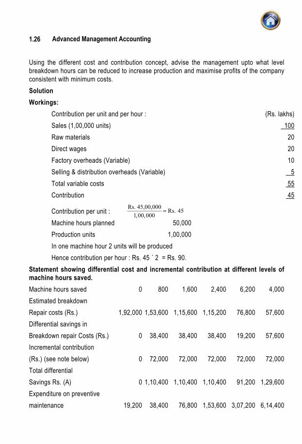
Advanced Management Accounting 1.26
Using the different cost and contribution concept, advise the management upto what level breakdown hours can be reduced to increase production and maximise profits of the company consistent with minimum costs. Solution Workings: Contribution per unit and per hour : (Rs. lakhs) Sales (1,00,000 units) 100 Raw materials 20 Direct wages 20 Factory overheads (Variable) 10 Selling & distribution overheads (Variable) 5 Total variable costs 55 Contribution 45
Contribution per unit : Machine hours planned 50,000 Production units 1,00,000 In one machine hour 2 units will be produced Hence contribution per hour : Rs. 45 ´ 2 = Rs. 90. Statement showing differential cost and incremental contribution at different levels of machine hours saved. Machine hours saved 0 800 1,600 2,400 6,200 4,000 Estimated breakdown Repair costs (Rs.) 1,92,000 1,53,600 1,15,600 1,15,200 76,800 57,600 Differential savings in Breakdown repair Costs (Rs.) 0 38,400 38,400 38,400 19,200 57,600 Incremental contribution (Rs.) (see note below) 0 72,000 72,000 72,000 72,000 72,000 Total differential Savings Rs. (A) 0 1,10,400 1,10,400 1,10,400 91,200 1,29,600 Expenditure on preventive maintenance 19,200 38,400 76,800 1,53,600 3,07,200 6,14,400
Rs. 45,00,000 Rs. 451,00,000
=

Development in the Business Environment 1.27
Differential expenditure on preventive maintenance (Rs.) (B) 0 19,200 38,400 76,800 1,53,600 3,07,200 Incremental profit (Rs.) (A–B) 0 91,200 72,000 33,600 –62,400 –1,77,600 Note : Incremental contribution is calculated by multiplying differential hours saved by contribution per hour i.e. 800 × Rs. 90 = Rs. 72,000 Recommendation : It may be observed from the above table that savings in machine hours upto 2,400 yields incremental profit. Beyond this level, the differential maintenance costs exceed the differential savings. Therefore, the management is advised to reduce the level of breakdown hours upto 1600 (4,000 – 2,000) or save 2,400 breakdown hours to increase production. AT his level, the company will be able to maximise profits consistent with minimum costs. Illustration A Ltd. produces and markets a range of consumer durable appliances. It ensures after sales service through X Ltd. The big appliances are serviced at customer’s residence while small appliances are serviced at workshop of X Ltd. The material supplied to X Ltd. is charged at cost at 10%. X Ltd. charges customers at 25% over the above price. For labour, the company receives 10% of the rate fixed for work done under the after-sales service agreement and 15% of the rate fixed in case of jobs not covered under the agreement from X Ltd. 60% by value of the total work undertaken by X Ltd. was for appliances and rest accounted for small appliances during the previous year. The company decides to carry out all or some of the work itself and has chosen one area in the first instance. During the previous year the company earned a profit of Rs. 2,16,000 as detailed below from X Ltd. for the area chosen:
Materials Labour Rs. Rs.
Under after –sales service agreement 60,000 1,00,000 For jobs not covered under the agreement 20,000 36,000
The company forecasts same value of work in that area for the ensuring period. The following three options are under consideration of the management: (1) To set up a local service Centre to provide service for small appliances only. The
existing system is to continue for big appliances. (2) To set up a local services Centre to provide service for big appliances only. The existing
system is to continue for small appliances. (3) To set up a local service Centre to provide service to all appliances. The existing system
then stands withdrawn.

Advanced Management Accounting 1.28
The relevant costs for carrying out jobs under the above options are as under: (Rs.’000)
Option -1 Option -2 Option -3
Heat, rent, light etc. 125 50 150 Management costs 108 83 150 Service staff costs 230 440 750 Transport costs 25 220 230
You are required to find out the most profitable option. Solution Statement showing value of total work undertaken by X Ltd. at customer’s price.
(Rs. ‘000) Material cost (for appliances covered under agreement) 825 [Refer to working note 1(i)] Material cost (for appliances not covered under agreement) 275 [Refer to working note 2(i)] Labour cost (for appliances covered under agreement) 1,000 Labour cost (for appliances not covered under agreement) 240 [Refer to working note 2(ii)] Total receipts 2,340 Break up of receipts: Big appliances 60% 1,404 Small appliances 40% 936 Profitability Statement (Rs.’000) Option 1 Option 2 Option 3 Income: Big appliances 129.6 1,404 1,404 (60%×Rs. 216) Small appliances 936 86.4 936 _____ (40%× Rs. 216) ______ Total receipts: (A) 1,065.6 1,490.4 2,340

Development in the Business Environment 1.29
Costs: Material 320 480 800 Heat, rent, light etc., 125 50 150 Management costs 108 83 150 Service staff costs 230 440 750 Transport costs 25 220 230 Total costs: (B) 808 1,273 2,080 Profit: [(A-B)] 157.6 217.4 260 Recommendation: Option 3 is most profitable one. Working Notes: 1. Material and labour cost (for appliances under after sales agreement): Rs.
(i) Cost of Material per unit charged to customer’s by X Ltd. 137.50 (Rs. 100 +10% (Rs. 100+25%´Rs.110) cost of material charged to customer’s by X Ltd.
50.137.
10.000,60. xRs
RsRs
8,25,000 (ii) Cost of labour charged to customers by X Ltd.
100
10.000,00,1. x
RsRs
10,00,000 2. Material and labour cost (for appliances not covered under sales agreement): Rs.
(i) Cost of material charged to customers by X Ltd.
50.137.
10.000,20. xRs
RsRs
2,75,000 (ii) Cost of labour charged to customers by X Ltd.
100
15.000,36. x
RsRs
2,40,000

Advanced Management Accounting 1.30
1. 3 ACTIVITY BASED COST MANAGEMENT 1.3.1 Introduction Contrary to what might be imagined, many organisations do not wish to know how much it costs to make a product with precise accuracy. This is because pricing is based on what the market will bear, competitors’ moves, etc. Others however fix their price on cost and need to be able to determine it with reasonable accuracy. The latter organisations have been greatly benefitted from the development of activity based costing (ABC), which is a modern absorption costing method, It should not be assumed that all traditional absorption costing systems are not accurate enough to give adequate information for pricing purposes or other, long-run management decision purposes. Some traditional systems treat overheads in a detailed way and relate them to service cost centres as well as production cost centres. The service centre overheads are then spread over the production cost centres before absorption rates are calculated. The main cause of inaccuracy is in the calculation of the overhead rate itself, which is usually based on direct labour hours or machine hours. These rates assume that products that take longer to make, generate more overheads. Thus traditional cost system overcosted high volume products and undercost low volume products. Factors prompting the development of ABC system include : 1. Growing overhead costs because of increasingly automated production 2. Increasing market competition which necessitated more accurate product costs. 3. Increasing product diversity to secure economies of scope & increased market share. 4. Decreasing costs of information processing because of continual improvements and
increasing application of information technology 1.3.2 Meaning of ABC Activity Based Costing is an accounting methodology that assign costs to activities rather than products or services. This enables resources & overhead costs to be more accurately assigned to products & services that consume them. ABC assign cost to activities based on their use of resources. It then assign cost to cost objects, such as products or customers, based on their use of activities. ABC can track the flow of activities in organization by creating a link between the activity (resource consumption) and the cost object. The flow is characterized through four core areas :
• Cost object.
• Cost drivers.
• Resource Cost drivers.
• Activity Cost drivers.

Development in the Business Environment 1.31
In order to understand how ABC operates it is necessary to understand the meaning of above terms. 1.3.3 Definitions A Cost Object–It is an item for which cost measurement is required e.g. a product or a customer. A Cost Driver–It is a factor that causes a change in the cost of an activity. There are two categories of cost driver : A Resource Cost Driver–It is a measure of the quantity of resources consumed by an activity. It is used to assign the cost of a resource to an activity or cost pool. An Activity Cost Driver–It is a measure of the frequency and intensity of demand, placed on activities by cost objects. It is used to assign activity costs to cost objects. The cost driver for business functions viz., Research & Development and Customer Service are as below :
Business functions : Cost Driver Number of research products Personnel hours on a project Research & Development Technical complexities of projects Number of service calls Number of products serviced Customer Service Hours spent on servicing products.
In traditional costing overheads are first related to cost centres (Production & Service Centres) and then to cost objects, i.e., products. In ABC overheads are related to activities or grouped into cost pools (depending on the terminology preferred). Then they are related to the cost objects, e.g., products. The two processes are, therefore, very similar, but the first stage is different as ABC uses activities instead of functional departments (cost centres). The problem with functional departments is that they tend to include a series of different activities, which incur a number of different costs that behave in different ways. Activities also tend to run across functions; for instance, procurement of materials often includes raising a requisition note in a manufacturing department or stores. It is not raised in the purchasing department where most procurement costs are incurred. Therefore, ABC gives a more realistic picture of the way in which costs behave. As with traditional absorption costing ABC rates are calculated in advance, normally for a year ahead, and so the same rates are used for a year at a time. The advantage of this is that any seasonal variations will be spread giving an average cost. If this was not done and actual rates were used the absorption rates would vary monthly. This would mean that when output was high the overhead rate would be low and vice versa; if pricing were based on cost the prices quoted would be higher when the business was slack.

Advanced Management Accounting 1.32
1.3.4 Stages in Activity Based Costing The different stages in activity based costing are listed below and are shown in Figure (A) (1) Identification of the activities that may take place in an organisation : The first stage is to identify the major activities in the organization. There can be machine related activities, direct labour related activities and various support activities such as ordering, receving, material parts handling etc. Usually the number of cost centres that a traditional overhead system uses are quite small, say upto fifteen. In ABC the number of activities will be much more, say 200; the exact number will depend on how the management subdivides the organisation’s activities. It is possible to break the organisation down into many very small activities. But if ABC is to be acceptable as practical system it is necessary to use larger groupings, so that, say, 40 activities may be used in practice. The activities may be listed as follows:-Production schedule changes
• Customer liaison
• Purchasing
• Production process set up
• Quality control
• Material handling
• Maintenance (2) Assigning costs to cost pool for each activity both support and primary activities, that caused them. This creates ‘cost pools’ or ‘cost buckets’. This will be done using resource cost drivers that reflect causality. (3) Support activities are then spread across the primary activities on some suitable base, which reflects the use of the support activity. The base is the cost driver that is the measure of how the support activities are used. (4) Determine the cost drivers for each activity that will be used to relate the overheads collected in the cost pools to the cost objects/products. A cost Driver is a variable, which determines the work volume or work load of a particular activity. This is based on the factor that drives the consumption of the activity. The question to ask is – what causes the activity to incur costs ? In production scheduling, for example, the driver will probably be the number of batches ordered. Some questions which are aimed at bringing out the cost drivers are given below:-
• What is the number of staff working on a particular activity?
• Why is overtime worked?
• Why does the idle time occurs?
• What is it, that determines the amount of timew spent on a particular activity?

Development in the Business Environment 1.33
The end result of this type of questioning will be a typical set of cost drivers for each sub-activity. (5) Assigning the costs of activities to products according to product demand for activities : This step involves tracing the cost of the activities to products according to products demand for these activities during the production process. This requires to calculate cost driver rate for each activity, just as an overhead absorption rate would be calculated in the traditional system.
Activity cost driver rate =
Total cost activityActivitydriver
The activity driver rate can be used to cost products, as in traditional absorption costing, but it can also cost other cost objects such as customers/customer segments and distribution channels. The possibility of costing objects other than products is part of the benefit of ABC. The activity cost driver rates will be multiplied by the different amounts of each activity that each product/other cost object consumes. Cost flow in activity based costing
Resources : Staff wages Electricity Advertising (resource cost drivers) Support activities : i ii iii Primary activities : i ii iii (activity cost drivers) Cost objects : Products/ Customer Distribution services segments channels
Activities basically fall into four different categories, known as the manufacturing cost hierarchy. These categories are generally accepted today but were first identified by Cooper (1990). The categories of activities help to determine the type of activity cost driver required. The categories of activities are : 1. Unit level activities. The costs of some activities (mainly primary activities) are strongly correlated to the number of units produced. For example, the use of indirect materials/consumables tends to increase in proportion to the number of units produced. Another example of a unit level activity is the inspection or testing of every item produced, if this was deemed necessary or, perhaps more likely, every 100th item produced. 2. Batch level activities. The cost of some activities (mainly manufacturing support activities) are driven by the number of batches of units produced. Examples of this are :
• Material ordering–where an order is placed for every batch of production

Advanced Management Accounting 1.34
• Machine set-up costs–where machines need resetting between each different batch of production.
• Inspection of products–where the first item in every batch is inspected rather than every 100th item quoted above.
3. Product level activities. The costs of some activities (often once only activities) are driven by the creation of a new product line and its maintenance, for example, designing the product, producing parts specifications and keeping technical drawings of products up to date. Advertising costs fall into this category if individual products are advertised rather than the company’s name. 4. Facility level activities. Some costs cannot be related to a particular product line, instead they are related to maintaining the buildings and facilities. Examples are the maintenance of buildings, plant security, business rates, etc. Also included in this category are salaries, such as the production manager’s. Advertising campaigns that promote the organisation would also be included. The first and last categories above are the same as those in traditional absorption costing and so if an organisation costs are mainly made up of these two categories ABC, will not improve the overhead analysis greatly. But if the organisation’s costs fall mainly in the second and third categories an ABC analysis will provide a different and more accurate analysis. Illustration A company produces three products A, B and C for which the standard costs and quantities per unit are as follows :
Products A B C
Quantity produced 10,000 20,000 30,000 Direct material/p.u. (Rs.) 50 40 30 Direct labour/p.u. (Rs.) 30 40 50 Labour hours/p.u. 3 4 5 Machine hours/p.u. 4 4 7 No. of purchase requisitions 1,200 1,800 2,000 No. of set ups 240 260 300 Production overhead split by departments — Department 1 = Rs. 11,00,000 — Department 2 = Rs. 15,00,000 Department 1 is labour intensive and Department 2 is machine intensive Total labour hours in Department 1 = 1,83, 333 Total machine hours in Department 2 = 5,00,000

Development in the Business Environment 1.35
Production overhead split by activity— Receiving/inspecting Rs.14,00,000 — Production scheduling/machine set up Rs.12,00,000 Rs. 26,00,000 Number of batches received/inspected = 5,000 Number of batches for scheduling and set-up = 800 You are required to: (i) Prepare Product Cost Statement under traditional absorption costing and Activity Based
Costing method. (ii) Compare the results under two methods. Solution Traditional absorption costing Absorption rates :
Department 1 = Rs. 11,00,0001,83,333 labour hours
= Rs. 6 per labour hour
Department 2 = Rs. 15,00,000
5,00,000 machinehours = Rs. 3 per machine hour
Product cost statement Products A B C Rs. Rs. Rs. Direct materials 50 40 30 Direct labour 30 40 50 Overhead : Department 1 18 24 30 (3 hrs. × Rs. 6) (4 hrs. × Rs. 6) (5 hrs. × Rs. 6) Department 2 12 12 21 (4 hrs. × Rs. 3) (4 hrs. × Rs. 3) (4 hrs. × Rs. 7) Total cost p.u. 110 116 131 Activity based costing Cost driver rates :
Receiving/inspecting = Rs. 14,00,0005,000 (No. of batches received/inspected)
= Rs. 280 per requisition Production scheduling/Machine set ups = Rs. 1,500 per set up

Advanced Management Accounting 1.36
Product cost statement (per unit)
Products A B C Rs. Rs. Rs.
Direct materials (Rs. ) 50 40 30 Direct labour (Rs.) 30 40 50 Overhead : Receiving 34* 25 19 Production scheduling 36** 20 15
Total cost per unit 150 125 114
{Rs. 280 × 1,200} ÷ 10,000 units = Rs. 34*; similarly Rs. 25 and Rs.19 (Rs. 1,500 × 240) ÷ 10,000 units = Rs. 36**; similarly Rs. 20 and Rs. 15 The two absorption methods produce different results. Product C appears to be much more expensive using the traditional method than it does with ABC, while product A is the opposite. If it is assumed that ABC is more accurate, which it may or may not be, then product C would be overpriced on the traditional method and sales would presumably be poor as a consequence–assuming competitors supply more cheaply. Product A would be the opposite : sales would be high and it is possible that the company would unknowingly make a loss per unit on product A. Illustration The following information provides details of costs, volume & cost drivers for a particular period in respect of ABC. Ltd. for product X, Y and Z
Product X Product Y Product Z Total
1. Production and sales (units) 30,000 20,000 8,000 2. Raw material usage (units) 5 5 11 3. Direct material cost (Rs.) 25 20 11 12,38,000 4. Direct labour hours 1.33 2 1 88,000 5. Machine hours 1.33 1 2 76,000 6. Direct labour cost (Rs.) 8 12 6 7. Number of production runs 3 7 20 30 8. Number of deliveries 9 3 20 32 9. Number of receipts (2 × 7)* 15 35 220 270 10. Number of production orders 15 10 25 50
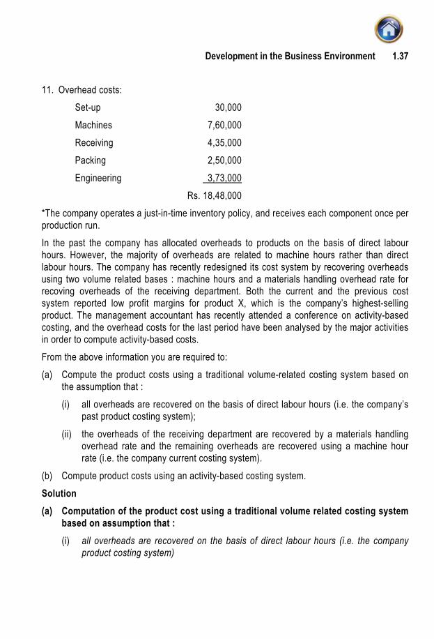
Development in the Business Environment 1.37
11. Overhead costs: Set-up 30,000 Machines 7,60,000 Receiving 4,35,000 Packing 2,50,000 Engineering 3,73,000 Rs. 18,48,000 *The company operates a just-in-time inventory policy, and receives each component once per production run. In the past the company has allocated overheads to products on the basis of direct labour hours. However, the majority of overheads are related to machine hours rather than direct labour hours. The company has recently redesigned its cost system by recovering overheads using two volume related bases : machine hours and a materials handling overhead rate for recoving overheads of the receiving department. Both the current and the previous cost system reported low profit margins for product X, which is the company’s highest-selling product. The management accountant has recently attended a conference on activity-based costing, and the overhead costs for the last period have been analysed by the major activities in order to compute activity-based costs. From the above information you are required to: (a) Compute the product costs using a traditional volume-related costing system based on
the assumption that : (i) all overheads are recovered on the basis of direct labour hours (i.e. the company’s
past product costing system); (ii) the overheads of the receiving department are recovered by a materials handling
overhead rate and the remaining overheads are recovered using a machine hour rate (i.e. the company current costing system).
(b) Compute product costs using an activity-based costing system. Solution (a) Computation of the product cost using a traditional volume related costing system
based on assumption that : (i) all overheads are recovered on the basis of direct labour hours (i.e. the company
product costing system)

Advanced Management Accounting 1.38
Statement showing the product cost
Products X Y Z Rs. Rs. Rs.
Direct labour 8 12 6 Direct materials 25 20 11 Overhead 28 42 21 (Refer to working note) (1.33 hrs. × Rs. 21) (2 hrs. × Rs. 21) (1 hr. × Rs. 21) Total 61 74 38
Working note : Overheads to be charged to products
Direct labour overhead rate = Total OHTotal DLH
= Rs. 21 per direct labour hour. (ii) The overheads of the receiving department are recovered by a material handling
overhead rate & the remaining overheads are recovered by using a machine hour rate (i.e. the company current costing system)
Products X Y Z Rs. Rs. Rs.
Direct labour 8 12 6 Direct materials 25 20 11 Material handling overhead 8.78 7.03 3.87 (Refer to working note) (Rs. 25 × 35.14%) (Rs. 20 × 35.14%) (Rs.11×35.14%) Other overheads 24.79 18.59 37.18 (machine hour basis) Refer to Working note :
Overheads to be charged to products :
Material handling overhead rate = Reveiving Dept. OHDirect material cost
= 35.14% of direct material cost.
Machine hour overhead rate = Other OHMachine Hrs.
= 18.59 per machine hours.

Development in the Business Environment 1.39
(b) Statement showing the product costs using an activity based costing system.
Products X Y Z Rs. Rs. Rs.
Direct labour 8 12 6 Direct materials 25 20 11 Machine overheads 13.33 10 20 (Refer to working note1) (1 hrs.× Rs. 10) (1 hr.× Rs.10) (2 hrs.×Rs. 10) Set-up costs 0.10 0.35 2.50 (Refer to working note 2(i)) Receiving 0.81 2.82 44.30 (Refer to working note 2(ii)) Packing 2.34 1.17 19.53 (Refer to working note 2(iii)) Engineering 3.73 3.73 23.31 (Refer to working note 2(iv)) Total manufacturing cost 53.31 50.07 126.64
Working note :
1. Machine overhead rate per hour = Rs. 7,60,00076,000 hrs.
= Rs. 10
2. The cost per transaction or activity for each of the cost centres is as follows : (i) Set-up cost
Cost per setup = Rs. 30,00030
= Rs. 10004
(ii) Receiving Cost
Cost per receiving order = Rs. 4,35,000270
= Rs. 1611
(iii) Packing Cost
Cost per packing order = Rs. 2,50,00032
= Rs. 7812
(iv) Engineering
Cost per production order =
Rs. 3,73,00050
= Rs. 7460

Advanced Management Accounting 1.40
1.3.5 Purposes and benefits of Activity Based Costing Initially companies switched from traditional absorption costing to ABC in order to produce more accurate cost information for products, as shown above. The managers in some of these companies were surprised by the information revealed which indicated inordinately high cost., This led them to adjust their pricing policies and to develop different product strategies, as they found that previously high volume, long production run products had been over-costed and low volume, short production run products under-costed. To summarise, ABC is particularly needed by organisations for product costing where:
• Production overheads are high in relation to direct costs
• There is a great diversity in the product range
• Products use very different amounts of the overhead resources
• Consumption of overhead resources is not primarily driven by volume. But if ABC is only considered to be a more detailed and accurate overhead absorption costing system many organisations may decide to do without it. Advocates of using ABC for a accurate overhead apportionment usually compare the ABC technique with the most basic traditional absorption costing system where one blanket overhead rate is applied. 1.3.6 Activity Based Cost system installation and operation The motives for pursuing an ABC implementation, or at least of investigating its feasibility, must be established at the outset. Most commonly these will be : 1. To improve product costing especially in those situations where existing methods under
cost some products and over cost others; or 2. To identify non-value-adding activities in the production process which might be a
suitable focus for attention or elimination. In practice, the former is the most quoted goal, even though the latter may be more appropriate. This is especially so for firms which are highly labour intensive and which do not have a great diversity of products in their range, and where allocation of overhead based on direct labour hours may already function efficiently. Direct costs, like materials and direct labour, are easily assigned directly to products. Some indirect costs, particularly those selling costs which are product specific (e.g., advertising), may be directly assigned to the product too. The remaining indirect costs are those which are problematical and provide the focus for ABC, with resource costs indirectly assigned to the cost object via cost pools and activity drivers. A number of distinct practical stages in the ABC implementation are as follows : 1. Staff training : The co-operation of the workforce is critical to the successful
implementation of ABC. They are closest to the process and most aware of the problems. Staff training should be, as far as possible, jargon-free, and create an awareness of the purpose of ABC. It should be non-threatening in nature, stressing that increased

Development in the Business Environment 1.41
efficiencies resulting from a successful implementation will mean rewards not redundancies. The need for the co-operation of staff in the concerted team effort, for mutual benefit, must be emphasised throughout the training activity.
2. Process specification : Informal, but structured, interviews with key members of personnel will identify the different stages of the production process, the commitment of resources to each, processing times and bottlenecks. The interviews will yield a list of transactions which may, or may not, be defined as ‘activities’ at a subsequent stage, but in any case provide a feel for the scope of the process in the entirety.
3. Activity definition : The problem must be kept manageable at this stage, despite the possibility of information overload from new data, much of which is in need of codification. The listed transactions must be rationalised in order to aggregate those in similar categories and eliminate those deemed immaterial. The resultant cost pools will likely have a number of different events, or drivers, associated with their incurrence.
4. Activity driver selection : A single driver covering all of the transactions grouped together in an ‘activity’ probably does not exist. Multiple driver models could be developed if the data were available, but cost-benefit analysis has rarely shown these to be desirable. The intercorrelation of potential activity drivers will probably be so strong as to suggest that it really does not matter which one is selected. This argument might be employed to avoid the costly collection of data items otherwise not monitored, nor easily accessible.
5. Costing : A single representative activity driver can be used to assign costs from the activity pools to the cost objects. If, for example, the number of engineering set-ups has been identified as a driver of process costs and the total set-up cost is Rs. 40,000 for a company producing four products (A, B, C, D) then the number of set-ups per product can be used to assign these costs. If product A requires 2 set-ups; B4 set-ups ; C24 and D10, then the average cost per set-up of Rs. 40,000/40 set ups = Rs. 1,000, a misleading figure taken at face value, which does not imply the different demands of the set up resource made by the different products. However, total set-up costs can be distributed to product groups in proportion to use, i.e., A : Rs. 2,000, B : Rs. 4,000, C : Rs. 24,000 and D : Rs. 10,000 and then assigned to individual units of product in proportion to the total level of output.
This procedure can then be repeated for all material activities. 1.3.7 Activity Based Cost Management (ABM) Empirical studies of ABC implementation have frequently shown that the greater benefit derived from its adoption is in Cost Management rather in providing accurate product cost. The term Activity based management (ABM) is used to describe the cost management application of ABC. The use of ABC as a costing tool to manage costs at activity level is known as Activity Based Cost Management (ABM). ABM is a discipline that focuses on the efficient and effective management of activities as the route to continuously improving the value received by customers. ABM utilizes cost information gathered through ABC. Through various analysis, ABM manages activities rather than resources. It determines what drives the

Advanced Management Accounting 1.42
activities of the organization and how these activities can be improved to increase the profitability. 1.3.7.1 Stages in Activity Based Cost Management : We have already discussed the various stages involved in activity based product costing. These stages are : 1. Identification of the activities that have taken place in the organisation. 2. Assigning costs to cost pool for each activity. 3. Spreading of support activities across the primary activities. 4. Determining cost driver for each activity. 5. Assigning the costs of activities to products according to product demand for activities. The application of ABC as a costing tool to manage cost requires the firm to omit the final stage of assigning costs to products and adopt activity based costing without activity based product costing. Alternatively, organisation can design an activity based system and incorporates both ABM and Activity Based Product Costing. 1.3.7.2 Activity Based Management Model : Consortium for Advanced Management International (CAM) defines ABM as “adds a dynamic, continuous improvement dimension to the more static ABC model.” Interestingly, it has been observed that Japanese accountants began exploring activity-based techniques in the early 1990s following movement in the United States toward the ABM model. CAM-1 defines ABM as : “A discipline that focuses on the management of activities as the route to improving the value received by the customer and the profit achieved by providing this value. This discipline includes cost driver analysis, activity analysis, and performance measurement. Activity-Based Management draws on Activity-Based Costing as its major source of information.” The fig.- 1 pictorially represents ABM model in a chart developed for CAM-1. In commenting on this model, one of its co-developers stated, “ABC supplies the information, and ABM uses this information in various analyses designed to yield continuous improvement.” (a) Cost Driver Analysis : The factors that cause activities to be performed need to be identified in order to manage activity costs. Cost driver analysis identifies these causal factors. For example, a cost driver analysis study might determine that slow processing of customer invoices results largely from lack of training of the customer invoice associates. This lack of training is thus a cost driver of the customer invoice processing activity. It is one of the factors causing this activity to take place (in this case, inefficiently). Managers have to address this cost driver to correct the root cause of the slow processing problem. To accomplish this task, managers might decide that an internal training program for customer invoice associates should be designed and implemented to increase the speed of customer invoice processing.

Development in the Business Environment 1.43
Fig. 1 : Activity-Based Management Model. Source : From the CAM-I Glossary of
Activity-Based Management, Edited by Norm Raffish and Peter B. B. Turney, (Arligton : CAM-I, 1991).
The time saving from the improved training may lead to a reduction in the number of customer invoice associated and, thus, to lower costs for the “customer invoice processing” activity. Of course, real salary cost savings occur only if the number of jobs in the organisation actually decreases (e.g., through attrition) or if displaced customer invoice associates are redeployed to VA activities, thus canceling the need to hire new employees from outside. The tangible cost savings and intangible benefits from the customer invoice processing improvements should be compared with both the tangible and intangible costs of the new training program in a cost-benefit analysis. The hypothetical customer invoice processing example shows that the identification and analysis of cost drivers (causal factors) is a necessary first step toward improving the cost-effectiveness of activities and cost management through ABM. (b) Activity Analysis : Activity analysis, defined in section (a), identifies the activities of an organisation and the activity centres (or activity cost pools) that should be used in an ABC system. Activity analysis also identifies VA and NVA activities. The degree to which activities are grouped together into activity centres depends on the costs and benefits of the alternatives. The number of activity centres is likely to change over time as organisational needs for activity information evolve. For example, only a few activity centres may be used in an initial ABC pilot study. As managers become more accustomed to the initial ABC system and find the output useful, they may request a more detailed and refined ABC model. (c) Performance Analysis : Performance analysis involves the identification of appropriate measures to report the performance of activity centres or other organisational units, consistent

Advanced Management Accounting 1.44
with each unit’s goals and objectives. Performance analysis aims to identify the best ways to measure the performance of factors that are important to organisations in order to stimulate continuous improvement. 1.3.7.3 Business application of ABM : ABM views the business as a set of linked activities that ultimately add value to the customer. ABM is based on the premise that activities consume costs. Therefore, by managing activities costs will be managed in long term. Activities may be grouped in such a way as to describe the total process. For example, serving a particular customer involves a number of discrete activities, but the sum total of these activities represents the process by which the client is serviced. ABM classifies each activity within a process as value-added activities or non-value added activities. Value-added activities (VA) : The value-added activities are those activities which are necessary for the performance of the process. Such activities represents work that is valued by the external or internal customer. The customers are usually willing to pay (in some way) for the service. For example polishing a furniture by a manufacturer dealing in furniture is value added activity. Non-value-added activities (NVA) : The NVA activity represents work that is not valued by the external or internal customer. NVA activities do not improve the quality or function of a product or service, but they can adversely affect costs and prices. Non-value added activities create waste, result in delay of some sort, add costs to the products or services and for which the customer is not willing to pay. Moving materials and machine set up for a production run are examples of NVA activities. For example, in the Internal Revenue Service department, rerouting documents and the wait or delay time in completing a case are examples of NVA activities in the “installment agreements” area. The preparation of tax returns and other compliance work by organisations do not directly benefit the customers of their products and services, but because they are required by law. They are not considered NVA activities. By measuring activities rather than traditional departmental costs, business can focus on cross functional processes in order to identify non-value adding activities and pinpoint the time drives of cost at each stage. The goal of the ABCM is to make customer needs to be satisfied while making fewer demands for resources. Current research suggests that customers have perceived needs in four areas, all of which must be satisfied simultaneously. The customers require: (i) Lower costs (ii) Higher quality (iii) Faster response time (iv) Greater innovation.

Development in the Business Environment 1.45
To satisfy these needs ABM currently being used for a variety of business applications. Such as: (i) Cost reduction : ABCM helps the organisation to identify costs against activities and to
find opportunities to streamline or reduce the costs or eliminate the entire activity, especially if there is no value added. It is particularly useful in identifying and quantifying process waste and providing vehicle for continuous process improvement through continuous cost reduction.
(ii) Activity Based Budgeting : Activity based budgeting analyse the resource input or cost for each activity. It provides a framework for estimating the amount of resources required in accordance with the budgeted level of activity. Actual results can be compared with budgeted results to highlight both in financial and non-financial terms those activities with major discrepancies from budget for potential reduction in supply of resources. It is a planning and control system which seeks to support the objectives of continuous improvement. It means planning and controlling the expected activities of the organization to derive a cost-effective budget, that meet forecast workload and agreed strategic goals. The three key elements of activity based budgeting are as follows:-
• Type of work to be done
• Quantity of work to be done
• Cost of work to be done (iii) Business process re-engineering : Business process re-engineering involves
examining business processes and making substantial changes to how organisation currently operates. ABCM is a powerful tool for measuring business performance, determining the cost of business output and is used as a means of identifying opportunities to improve process efficiency and effectiveness. A business process consist of linked set of activities. For example purchasing of materials might be considered as business process consist of activities such as receiving a purchase request, identifying supplies, preparing purchase orders, mailing purchase orders and performing follow up. The process might be reengineered by sending the production schedule direct to the suppliers and to enter into contractual agreement to deliver materials according to the production schedule. The end result might be permanent reduction or elimination of some activities.
(iv) Benchmarking : This aspect has been discussed later in chapter 14 of this book. (v) Performance measurement :Many organisations are now focussing on activity
performance as a means of facing competitors and managing costs. To monitor efficiency and effectiveness of activities performance measures are required. Activity performance measures consist of measures relating to costs, time, quality and innovation. For instance, now-a days in the globalisation the overall goal which is significant for a company is to produce a quality product at a price that will be competitive in world market. But the quality is not something which one can apply somewhere in the production process or assume will happen automatically. Product quality starts with the

Advanced Management Accounting 1.46
correct design. The next stages are high quality raw material inputs, quality processing and work, and proper handling and packaging etc. The various performance measures of quality are :
Area Measures quality of purchased component zero defects quality of output % yield customer awareness orders; number of complaints 1.3.7.4 Benefits of Activity Based Cost Management (i) Provision of excellent basis and focus for cost reduction. (ii) Provides operational management with a clear view of HOW to implement an Activity
Based budget. (iii) Provision of clear understanding of the underlying causes of business processing costs. (iv) Provision of excellent basis for effectiveness of management decision making. (v) Identification of key process waste elements permit management prioritisation and
leverage of key resources 1.3.8. Difference between ABC and ABM The ABC refers to the technique for determining the cost of activities and the output that those activities produce. It is the logical distribution of overhead i.e. overhead should be distributed on the consumption of resources consumed by goods and services. The aim of ABC is to generate improved cost data for use in managing a company’s activities. The ABM is a much broader concept. It refers to the management philosophy that focuses on the planning, execution and measurement of activities as the key to competitive advantage. 1.3.9. ABC : A Decision Making Tool It is a useful tool for many of the management decisions facing companies today. It can bring a picture of the operation to light that may not be obvious through other analysis tools. Specifically, ABC is useful in analyzing specific segments of an organization. This might include a market line, a group of products (even a single product), a customer, or an employee. The ABC is implemented in following decisions: 1. ABC is a complement to total quality management (TQM). It provides quantitative data
that can track the financial impact of improvements implemented as part of the TQM initiative. Some have even suggested that ABC is the most important concept introduced since TQM. Amoco Performance Products, Transparent Container Co. and Fellowes Manufacturing Co. are a few companies that have utilized the ABC/TQM modeling concept to improve performance and profitability.
2. Wholesale distributors can gain significant advantage in the decision-making process through implementation of ABC concepts. The expansion of line offerings has brought

Development in the Business Environment 1.47
about difficult decisions for the distributor. Using traditional financial data, overhead burden is distributed equally across the product line.
Introduction of new products or vendors might also introduce variance to the overhead. For instance, the need to support a special storage area for control or environmental reasons, or the need of new handling equipment will increase overall operational costs. These costs will be spread over the product line, reducing margin on existing products and reducing the cost impact of the new items. ABC models the costs back to the activity. The burden created by the new product is correctly reflected. This allows the existing merits while leaving the new line to justify itself.
3. Other decisions that can be assisted by ABC include facility and resource expansion. Often the basis for relocation or opening of a new distribution center is based on cost associations. Reduction in freight or other logistics costs can offset the expense of the new facility, staff or equipment. When the numbers used are enterprise-based, the return might not develop as expected. The ABC model can identify the specific cost elements being targeted, providing a much clearer picture from which management can act.
4. Decision support for human resources can be augmented by ABC. Where activity, and therefore cost, can be associated to an individual, new levels of financial performance can be determined. This might be appropriate in cases of branch management or sales. Adding or deleting resource slots can be determined based on costs of activities as well. The added data provided through ABC can present a number of options, including outsourcing, productivity improvements through automation, and a determination of employee/revenue ratios.
In summary, activity-based costing is a management decision-making tool. It provides financial support data structured in a fashion fundamentally different from accounting data provided in the general ledger. By associating cost to the activity, a clear relationship can be established between sources of activity demand and the related costs. This association can benefit the distributor in determining where costs are being incurred, what is initiating the costs and where to apply efforts to curb inflationary costs. This can be of particular value in tracking new products or customers. It can also provide tracking of logistics costs, one of the fastest growing areas of expense to the distribution operation.
1.3.10 Activity Based Budgeting (ABB) Activity-based budgeting is a process of planning and controlling the expected activities for the organisation to derive a cost-effective budget that meets forecast workload and agreed strategic goals. An activity-based budget is a quantitative expression of the expected activities of the firm, reflecting management’s forecast of workload and financial and non-financial requirements to meet agreed strategic goals and planned changes to improve performance. Thus, the key elements of ABB are: • type of work/activity to be performed; • quantity of work/activity to be performed; and • cost of work/activity to be performed.

Advanced Management Accounting 1.48
ABB focuses on the activity/business processes. Resources required are determined on the expected activities and workload. The objective is to bring in efficiency into the system. So, in the process of budget preparation, many key questions, need to be addressed and properly answered Illustration Having attended a CIMA course on activity-based costing (ABC) you decide to experiment by applying the principles to the four products currently made and sold by your company. Details of the four products and relevant information are given below for one period:
Product A B C D Output in units 120 100 80 120 Costs per unit Rs. Rs. Rs. Rs. Direct material 40 50 30 60 Direct labour 28 21 14 21 Machine hours (per unit) 4 3 2 3 The four products are similar and are usually produced in production runs of 20 units and sold in batches of 10 units. The production overhead is currently absorbed by using a machine hour rate, and the total of the production over head has been analysed as follows: Rs. Machine department costs (rent, Business, rates, depreciation and Supervision) 10,430 Set-up costs 5,250 Stores receiving 3,600 Inspection/quality control 2,100 Material handling and dispatch 4,620 You have identified ‘cost drivers’ to be used are as listed below for the overhead costs shown: Cost Cost Set-up costs Number of production runs Stores receiving Requisitions raised Inspection/quality control Number of production runs Materials handling and dispatch Orders executed The number of requisitions raised on the stores was 20 for each product and the number of orders executed was 42, each order being for a batch of 10 of a product.

Development in the Business Environment 1.49
Requirements (a) Calculate the total costs for each product if all overhead costs are absorbed on a
machine hour basis. (b) Calculate the total cost of each product, using activity-based costing. (c) Calculate and list the unit product costs from your fingers in (a) and (b) above, to show
the differences and comment briefly on any conclusions which may be drawn which could have pricing and profit implications.
Solution (a) Overheads absorbed on machine hour basis
Machine hour absorption rate = Total OverheadsTotal machine hours
=Rs.10,430+Rs.5,250+Rs.3,600+Rs.2,100+Rs.4,620 (120 X 4)+ (100 X 3)+(80 X 2)+(120 X 3) = Rs.26,000 = Rs.20 per machine hour 1,300 Total costs based on machine hour basis A B C D Rs. Rs. Rs. Rs. Direct material 40 50 30 60 Direct labour 28 21 14 21 Production overhead 80 60 40 60 Production cost/unit 148 131 84 141 Out put in units 120 100 80 120 Total production cost Rs.17,760 Rs.13,100 Rs.6,720 Rs.16,920 (b) Overheads absorbed based on ABC Overhead costs Level of activity Cost/activity Rs. Machine department costs 10,430 1,300 8.02/hour Set-up costs 5,250 21* 250.0/run Stores receiving costs 3,600 80** 45.00/requisition Inspection/quality costs 2,100 21* 100.00/run Material handling and dispatch 4,620 42 110.00/order

Advanced Management Accounting 1.50
Workings *No. of production runs = output in units/20 120+100+80 120
20 420 2120
=
A B C D Rs. Rs. Rs. Rs.
Direct materials 40.00 50.00 30.00 60.00 Direct labour 28.00 21.00 14.00 21.00 Machine dept costs 32.09 24.07 16.05 24.07 Set-up costs 12.50 12.50 12.50 12.50 Stores receiving 7.50 9.00 11.25 7.50 Inspection 5.00 5.00 5.00 5.00 Material handling 11.00 11.00 11.00 11.00 Production cost/unit 136.09 132.57 99.80 141.07
Output in units 120 100 80 120 Total production costs Rs.16,331 Rs.13257 Rs.7,984 Rs.16,928
(c) Comparison of the two unit costs calculated in (a) and (b) above,
A B C D Product Rs. Rs. Rs. Rs.
Based on machine Hour rate 148.00 131.00 84.00 141.00 ABC method 136.09 132.57 99.80 141.07 Difference 11.91 (1.57) (15.80) (0.07)
Illustration ABC Electronics Ltd makes audio player model AB 100. This model has 80 components. ABC sells 10,000 units each month at Rs. 3,000 per unit. The cost of manufacturing is Rs. 2,000 per unit or Rs. 200 lakhs per month for the production of 10,000 units. Monthly manufacturing costs incurred (in Rs. Lakhs) are as follows:

Development in the Business Environment 1.51
Direct materials costs 100.00 Direct manufacturing labour costs 20.00 Machining costs 20.00 Testing costs 25.00 Rework costs 15.00 Ordering costs 0.20 Engineering costs 19.80 Labour is paid on piece rate basis, therefore, ABC considers, direct manufacturing labour costs as variable cost. The following additional information is available for AB 100:
• Testing and inspection time per unit is 2 hours
• 10 per cent of AB 100 manufactured are reworked
• It currently takes 1 hour to manufacture each unit of AB 100. ABC places two orders per month for each component, each component being supplied by a different supplier.. ABC has identified activity cost pools and cost drivers for each activity. The cost per unit of the driver for each activity cost pool is as follows:
Manufacturing Description of activity cost driver cost per unit cost driver Machining costs Machining components Machine hours of Rs. 200 Capacity Testing costs Testing components and Testing hours Rs. 125 finished Products. (each unit of AB 100 is Tested individually) Rework costs Correcting and fixing errors Units reworked Rs. 1,500 Ordering costs Ordering of components Number of orders Rs. 125 Engineering costs Designing and managing of Engineering hrs. Rs. 198 Products and processes Over a long – run horizon, each of the overhead costs described above varies with chosen cost drivers. In response to competitive pressure ABC must reduce the price of its product to Rs. 2,600 and to reduce the cost by at least Rs. 400 per unit. ABC does not anticipate increase in sales due to price reduction. However, if it does not reduce price it will not be able to maintain the current sales level.

Advanced Management Accounting 1.52
Cost reduction on the existing model is almost impossible. Therefore, ABC has decided to replace AB 100 by a new model AB 200, which is a modified version of AB 100. the expected effect of design changes are:
• The number of components will be reduced to 50.
• Direct materials costs to be lower by Rs. 200 per unit.
• Machining time labour costs to be lower by 20%.
• Direct Manufacturing labour costs to be lower by Rs. 20 per unit.
• Testing time required to be low by 20%.
• Rework to decline to 5%
• Machining capacity and engineering hours capacity to remain the same. ABC currently outsource the rework on defective units. Required: • Compare the manufacturing cost per unit of AB 100 and AB 200.
• Determine the immediate effect of design change and pricing decision on the operating income of ABC.
Ignore income tax. Assume that the cost per unit of each cost driver for AB 100’ continues to apply to ‘AB 200. Solution Units AB-100 AB-200 10,000 10,000 Rs./unit Rs./unit Material 100 lakhs/10,000 1,000 800 Direct wages 20 L¸10,000 200 180 MC cost 200 160 Test cost 250 200 Rework cost 150 75 Ordering cost 2 1.25 Engineering cost 198 198 Total cost 2,000 1,614.25 Revised SP 2,600 2,600 Profit p.u 600 985.75 Total profit (Rs. In lakhs) 60 98.75

Development in the Business Environment 1.53
If the current products AB-100 is not replaced by new products AB-200 then profit will reduce by 38.75 lakhs. So, it is recommended to introduce AB-200.
1.4 TARGET COSTING 1.4.1 Introduction Target costing has been described as a process that occurs in a competitive environment, in which cost minimization is an important component of profitability. This newer approach of product costing may take into account initial design and engineering costs, as well as manufacturing costs, plus the costs of distribution, sales and services. 1.4.3.2 Definitions of Target Costing : It can be defined as “a structured approach to determining the cost at which a proposed product with specified functionality and quality must be produced, to generate a desired level of profitability at its anticipated selling price”. A critical aspect of this definition is that it emphasizes that target costing is much more than a management accounting technique. Rather, it is an important part of a comprehensive management process aimed at helping an organization to survive in an increasingly competitive environment. In this sense the term “target costing” is a misnomer: it is not a product costing system, but rather a management technique aimed at reducing a product’s life-cycle costs. 1.4.2 Advantages of Target Costing
1. It reinforces top-to-bottom commitment to process and product innovation, and is aimed at identifying issues to be resolved, in order to achieve some competitive advantage.
2. It helps to create a company’s competitive future with market-driven management for designing and manufacturing products that meet the price required for market success.
3. It uses management control systems to support and reinforce manufacturing strategies; and to identify market opportunities that can be converted into real savings to achieve the best value rather than simply the lowest cost.
1.4.3 Main features of Target Costing System The main features or practices followed in different Japanese companies can be understood by going through the following points :
1. Target costing is viewed as an integral part of the design and introduction of new products. As such, it is part of an overall profit management process, rather than simply a tool for cost reduction and cost management. Diagram 1 summarizes the steps in the target costing process. The first part of the process is driven by customer, market and profitability considerations. Given that profitability is critical for survival, a target profit margin is established for all new product offerings. The target profit margin is derived from the company’s long-term business plan, which incorporates its long-term strategic intent and profit margins. Each product or product line is required to earn at least the target profit margin.

Advanced Management Accounting 1.54
2. For any given product, a target selling price is determined using various sales forecasting techniques. Critical to setting the target selling price are the design specifications (reflecting certain levels of functionality and quality) of the new product. These specifications are based on customer requirements and expectations and are often influenced by the offerings of competitors. Importantly, while setting the target selling price, competitive conditions and customers’ demands for increased functionality and higher quality, without significant increases in price, are clearly recognized, as charging a price premium may not be sustainable. Hence, the target selling price is market-driven and should encompass a realistic reflection of the competitive environment.
3. Integral to setting the target selling price is the establishment of target production volumes, given the relationship between price and volume. The expected targets volumes are also critical to computing unit costs, especially with respect to capacity-related costs (such as tooling costs), as product costs are dependent upon the production levels over the life cycle of the product. Once the target selling price and required profit margin have been determined, the difference between these two figures indicates the allowable cost for the product. Ideally, the allowable cost becomes the target cost for the product. However, in many cases the target cost agreed upon will exceed the allowable cost, given the realities associated with existing capacities and capabilities.

Development in the Business Environment 1.55
4. The next stage of the target costing process is to determine cost reduction targets. Some firms will do this by estimating the “current cost” of the new product. The current cost is based on existing technologies and components, but encompasses the functionalities and quality requirements of the new product. The difference between the current cost and the target cost indicates the required cost reduction that is needed. This amount may be divided into a target cost-reduction objective and a strategic cost-reduction challenge. The former is viewed as being achievable (yet still a very challenging target), while the latter acknowledges current inherent limitations. After analysing the cost reduction objective, a product-level target cost is set which is the difference between the current cost and the target cost-reduction objective.
5. It should be noted that a fair degree of judgement is needed where the allowable cost and the target cost differ. As the ideal is to produce at the allowable cost, it is important that the difference is not too great. Once the product-level target cost is set, however, it generally cannot be changed, and the challenge for those involved is to meet this target.
6. Having achieved consensus about the product-level target cost, a series of intense activities commence to translate the cost challenge into reality. These activities continue throughout the design stage up until the point when the new product goes into production. Typically, the total target is broken down into its various components, each component is studied and opportunities for cost reductions are identified. These activities are often referred to as value engineering (VE) and value analysis (VA). Value engineering involves searching for opportunities to modify the design of each component or part of a product to reduce cost, but without reducing functionality or quality of the product. Value analysis entails studying the activities that are involved in producing the product to detect non-value-adding activities that may be eliminated or minimized to save costs, but without reducing the functionality or quality of the product. Where components are sourced from suppliers (which is often the case in the automotive industry), target prices are established for each part and the company’s employees work with the suppliers to ensure that the targets are achieved. Overall, the aim of the process is to ensure that when production commences, the total cost will meet the target, and profit goals will be achieved. There is also an ongoing continuous improvement program, known as kaizen costing, that focuses on the reduction of waste in the production process, thereby further lowering costs below the initial targets specified during the design phase.
While the above description captures the essential features of the target costing process, it should be emphasized that successful, target costing requires careful planning, attention to detail and a strong degree of commitment from those involved. The description, however, does not provide any insights into what is entailed in implementing a target costing approach in an organization. Here are some of the issues that are dealt with during a value engineering review :
1. Can we eliminate functions from the production process ? This involves a detailed review of the entire manufacturing process to see if there are any steps, such as interim quality reviews, that add no value to the product. By eliminating them, one can take their associated direct or overhead costs out of the product cost. However, these functions

Advanced Management Accounting 1.56
were originally put in for a reason, so the engineering team must be careful to develop work-around steps that eliminate one or more activities from the original set of functions.
2. Can we eliminate some durability or reliability ? It is possible to design an excessive degree of sturdiness into a product. For example, a vacuum cleaner can be designed to withstand a 1-ton impact, although there is only the most vanishing chance that such an impact will ever occur; designing it to withstand an impact of 100 pounds may account for 99.999% of all probable impacts, while also eliminating a great deal of structural material from the design. However, this concept can be taken too far, resulting in a visible reduction in durability or reliability, so any designs that have had their structural integrity reduced must be thoroughly tested to ensure that they meet all design standards.
3. Can we minimize the design ? This involves the creation of a design that uses fewer parts or has fewer features. This approach is based on the assumption that a minimal design is easier to manufacture and assemble. Also, with fewer parts to purchase, less procurement overhead is associated with the product. However, reducing a product to extremes, perhaps from dozens of components to just a few molded or prefabricated parts, can result in excessively high costs for these few remaining parts, since they may be so complex or custom made in nature that it would be less expensive to settle for a few extra standard parts that are more easily and cheaply obtained.
4. Can we design the product better for the manufacturing process ? Also known as design for manufacture and assembly (DFMA), this involve the creation of a product design that can be created in only a specific manner. For example, a toner cartridge for a laser printer is designed so that it can be successfully inserted into the printer only when the sides of the cartridge are correctly aligned with the printer opening; all other attempts to insert the cartridge will fail. When used for the assembly of an entire product, this approach ensures that a product is not incorrectly manufactured or assembled, which would call for a costly disassembly or (even worse) product recalls from customers who have already received defective goods.
5. Can we substitute parts ? This approach encourages the search for less expensive components or materials that can replace more expensive parts currently used in a product design. It is becoming an increasingly valid approach since new materials are being developed every year. However, sometimes the use of a different material impacts the types of materials that can be used elsewhere in the product, which may result in cost increases in these other areas, for a net increase in costs. Thus, any parts substitution must be accompanied by a review of related changes elsewhere in the design. This step is also known as component parts analysis and involves one extra activity—tracking the intentions of suppliers to continue producing parts in the future; if parts will not be available, they must be eliminated from the product design.
6. Can we combine steps ? A detailed review of all the processes associated with a product sometimes reveals that some steps can be consolidated, which may mean that one can be eliminated (as noted earlier) or that several can be accomplished by one person, rather than having people in widely disparate parts of the production process perform them. This is also known as process centering. By combining steps in this

Development in the Business Environment 1.57
manner, we can eliminate some of the transfer and queue time from the production process, which in turn reduces the chance that parts will be damaged during these transfers.
7. Is there a better way ? Though this step sounds rather vague, it really strikes at the core of the cost reduction issue—the other value engineering steps previously mentioned focus on incremental improvements to the existing design or production process, whereas this one is a more general attempt to start from scratch and build a new product or process that is not based in any way on preexisting ideas. Improvements resulting from this step lend to have the largest favourable impact on cost reductions but can also be the most difficult for the organization to adopt, especially if it has used other designs or systems for the production of earlier models.
Another approach to value engineering is to call on the services of a company’s suppliers to assist in the cost reduction effort. These organizations are particularly suited to contribute information concerning enhanced types of technology of materials, since they may specialize in areas that a company has no information about. They may have also conducted extensive value engineering for the components they manufacture, resulting in advanced designs that a company may be able to incorporate into its new products. Suppliers may have also redesigned their production processes, or can be assisted by a company’s engineers in doing so, producing cost reductions or decreased production waste that can be translated into lower component costs for the company. A mix of all the value engineering steps noted above must be applied to each product design to ensure that the maximum permissible cost is safely reached. Also, even if a minimal amount of value engineering is needed to reach a cost goal, one should conduct the full range of value engineering analysis anyway, since this can result in further cost reductions that improve the margin of the product or allow management the option of reducing the product’s price, thereby creating a problem for competitors who sell higher-priced products. Another term mentioned in the earlier explanation of the target costing process is “kaizen costing.” This is a Japanese term for a number of cost reduction steps that can be used subsequent to issuing a new product design to the factory floor. Some of the activities in the kaizen costing methodology include the elimination of waste in the production, assembly, and distribution processes, as well as the elimination of work steps in any of these areas. Though these points are also covered in the value engineering phase of target costing, the initial value engineering may not uncover all possible cost savings. Thus, kaizen costing is really designed to repeat many of the value engineering steps for as long as a product is produced, constantly refining the process and thereby stripping out extra costs. The cost reductions resulting from kaizen costing are much smaller than those achieved with value engineering but are still worth the effort since competitive pressures are likely to force down the price of a product over time, and any possible cost savings allow a company to still attain its targeted profit margins while continuing to reduce cost. This concept is illustrated in Exhibit 1. Of particular interest in Exhibit 1 is the use of multiple generations of products to meet the challenge of gradually reducing costs. In the example the market price continues to drop over time, which forces a company to use both target and kaizen costing to reduce costs and retain

Advanced Management Accounting 1.58
its profit margin. However, prices eventually drop to the point where margins are reduced, which forces the company to develop a new product with lower initial costs (Version B in the example) and for which kaizen costing can again be used to further reduce costs. This pattern may be repeated many times as a company forces its costs down through successive generations of products. The exact timing of a switch to a new product is easy to determine well in advance since the returns from kaizen costing follow a trend line of gradually shrinking savings and prices also follow a predictable downward track, plotting these two trend lines into the future reveals when a new generation of product must be ready for production. The type of cost reduction program used for target costing has an impact on the extent of cost reduction, as well as on the nature of the components used in a product. When a design team elects to set cost reduction goals by allocating specific cost reduction amounts to major components of an existing product, it tends to focus on finding ways to make incremental cost reductions rather than focusing on entirely new product configurations that might both radically alter the product’s design and lower its cost. This approach is most commonly used during the redesign of products already in the market. Another cost reduction approach is to allocate cost reductions based on the presence of certain product features in a product design. This method focuses the attention of the design team away from using the same components that were used in the past, which tends to produce more radical design changes that yield greater cost savings. However, the latter approach is also a riskier one, since the resulting product concepts may not work, and also requires so much extra design work that the new design may not be completed for a long time. Therefore, the second method is generally reserved for situations where a company is trying to create products at a radically lower cost than previously.
All the changes noted in this section that are necessary for the implementation and use of the target costing methodology represent a massive change in mind-set for the product design personnel of any company because they require the constant cooperation of many departments and rapid, voluminous communications between them, not to mention heightened

Development in the Business Environment 1.59
levels of trust in dealing with suppliers. All these concepts run counter to the traditional approach. It is no coincidence that the traditional design process defines each of the departments that take part in the process. These departments tend to guard their turf jealously, which is a major impediment to realizing a smoothly functioning set of product development teams. Only the most active support from senior management can enforce the new approach of drawing product design team members from all these castles and having them work together amicably. 1.4.6 Problems with Target Costing Though the target costing system results in clear, substantial benefits in most cases, it has a few problems that one should be aware of and guard against. These problem are as follows : 1. the development process can be lengthened to a considerable extent since the design
team may require a number of design iterations before it can devise a sufficiently low-cost product that meets the target cost and margin criteria. This occurrence is most common when the project manager is unwilling to “pull the plug” on a design project that cannot meet its costing goals within a reasonable time frame. Usually, if there is no evidence of rapid progress toward a specific target cost within a relatively short period of time, it is better to either ditch a project or at least shelve it for a short time and then try again, on the assumption that new cost reduction methods or less expensive materials will be available in the near future that will make the target cost an achievable one.
2. a large amount of mandatory cost cutting can result in finger-pointing in various parts of the company, especially if employees in one area feel they are being called on to provide a disproportionately large part of the savings. For example, the industrial engineering staff will not be happy if it is required to completely alter the production layout in order to generate cost savings, while the purchase staff is not required to make any cost reductions through supplier negotiations. Avoiding this problem requires strong interpersonal and negotiation skills on the part of the project manager.
3. representatives from number of departments on the design team can sometimes make it more difficult to reach a consensus on the proper design because there are too many opinions regarding design issues. This is a major problem when there are particularly stubborn people on the design team who are holding out for specific product features. Resolving out is difficult and requires a strong team manager, as well as a long-term commitment on the part of a company to weed out those who are not willing to act in the best interests of the team.
For every problem area outlined have the dominant solution is retaining strong control over the design teams, which calls for a good team leader. This person must have an exceptional knowledge of the design process, good interpersonal skills, and a commitment to staying within both time and cost budgets for a design project. 1.4.6 Cost Accountant’s Role in a Target Costing Environment 1. The cost accountant should be able to provide for the other members of the design team
a running series of cost estimates based on initial designs sketch, activities based

Advanced Management Accounting 1.60
costing reviews of production processes, and “best guess” costing information from suppliers based on estimated production volumes. Essentially in the earliest stages of a design, the cost accountant works with vague costing information and so must be able to provide estimates within a high-low range costs, gradually tightening this estimated cost range as more information becomes available.
2. The cost accountant should also be responsible for any capital budgeting requests generated by the design team since he or she has the knowledge of the capital budgeting process, how to fill out the required forms, and precisely what types of equipment are needed for the anticipated product design. The cost accountant also becomes the key contact on the design team for answers to any questions from the finance staff regarding issues or uncertainties in the capital budgeting proposal.
3. The cost accountant should work with the design team to help it understand the nature of various costs (such as cost allocations based on an activity-based costing system), as well as the cost-benefit trade-offs of using different design or cost operations in the new product.
4. In addition, the cost accountant is responsible for tracking the gap between the current cost of a product design and the target cost that is the design team’s goal, providing an itemization of where cost savings have already been achieved and where there has not been a sufficient degree of progress.
5. Finally, the cost accountant must continue to compare a product’s actual cost to the target cost after the design is completed, and for as long as the company sells the product. This is a necessary step because management must know immediately if costs are increasing beyond budgeted levels and why these increases are occurring.
There are particular qualifications that a cost accountant must have to be assigned to a target costing team. Certainly, one is having a good knowledge of company products as well as their features and components. Also, the cost accountant must know how to create an activity based costing system to evaluate related production costs, or at least interpret such costing data developed by someone else. Further, he or she must work well in a team environment, proactively assisting other members of the team in constantly evaluating the costs of new design concepts. In addition, he or she should have good analytical and presentation skills, since the ongoing costing results must be continually presented not only to other members of the team but also to the members of the milestone review committee. Thus, the best cost accountant for this position is an outgoing person with several years of experience within a company or industry. 1.4.7 Impact of Target Costing on Profitability Target costing can have a startlingly large positive impact on profitability, depending on the commitment of management to its use, the constant involvement of cost accountants in all phases of a product’s life cycle, and the type of strategy a company follows.

Development in the Business Environment 1.61
Target costing improves profitability in two ways. 1. It places such a detailed continuing emphasis on product costs throughout the life cycle
of every product that it is unlikely that a company will experience runaway costs; also, the management team is completely aware of costing issues since it receives regular reports from the cost accounting members of all design teams.
2. It improves profitability through precise targeting of the correct prices at which the company feels it can field a profitable product in the marketplace that will sell in a robust manner. This is opposed to the more common cost-plus approach under which a company builds a product, determines its cost, tacks on a profit and then does not understand why its resoundingly high price does not attract buyers. Thus, target costing results not only in better cost control but also in better price control.
Target costing is really part of a larger concept called concurrent engineering, which requires participants from many departments to work together on project teams rather than having separate departments handle new product design only after they have been handed off from the preceding department in the design chain. Clustering representatives from many departments together on a single design team can be quite a struggle, especially for older companies that have a history of conflict between departments. Consequently, only the most involved, prolonged support by all members of the senior management group can ensure that target costing and the greater concept of concurrent engineering, will result in significant profitability improvements. The review of product costs under the target costing methodology is not reserved just for the period up to the completion of design work on a new product. On the contrary, there are always opportunities to control costs after the design phase is completed, though these opportunities are fewer than during the design phase. Therefore, cost accountants should not be pulled from a design team once the final drawings have left the engineering department. Instead, they should regularly monitor actual component costs and compare them to planned costs, warning management whenever significant adverse variances arise. Also, cost accountants should take a lead role in the continuing review of supplier costs to see if they can be reduced, perhaps by visiting supplier facilities, as well as constantly reviewing existing product designs to see if they can be improved, and by targeting for elimination waste or spoilage on the production floor. Therefore, the cost accounting staff must be involved in all phases of a product’s life cycle if a company is to realize profitability improvements from target costing to the fullest extent. A company’s strategy can also has its impact on profitability. If it constantly issues a stream of new products, or if its existing product lines is subject to severe pricing pressure, it must make target costing a central part of its strategy so that the correct price points are used for products and actual costs match those originally planned. However, there are other strategies, such as growth by geographical expansion of the current product line (as is practised by retail stores) or growth by acquisition, where there is no particular need for target costing—these companies make their money in other ways than by a focused concentration on product features and costs. For them, there may still be a role for target costing, but it is strictly limited by the reduced need for new products.

Advanced Management Accounting 1.62
If the issues presented here are properly dealt with by a management team, it should find that target costing is one of the best accounting methods available for improving profitability. It is indeed one of the most pro-active systems found in the entire range of accounting knowledge. 1.4.9 Target Costing Data Flow 1. Data can be obtained from central accounting data base carefully stocked form such a
variety of sources as accounts payable, billing, bills of materials and inventory records. 2. In initial stages of product design, the cost accountant must make the best possible
guesses regarding the cost of proposed designs. 3. The cost accountant may include the best estimate an additional estimate of the highest
possible cost that will be encountered. This additional information lets management know whether there is a significant degree of risk that the project may not achieve its desired cost target.
4. Data can also be obtained from competitors information collected by the marketing staff or an outside research agency. This database contains information about the prices at which competitors are selling their products, as well as the prices of ancillary products and perhaps also the discounts given at various price points. It can also include market share data for individual products or by firm, the opinion of customers regarding the offerings of various companies, and the financial condition of competitors. This information is mostly used to determine the range of price points at which a company should sell its existing or anticipated products,
5. Sometimes information is compiled by a combined effort of the marketing and engineering staffs through a process called reverse engineering.This source can also serve as a data base for the project team.
6. Engineering staff also compiles their own cost data relating to different designs/components.This data is collected over the years and can be useful fior target costing.
7. The final database available to the cost accounting member of a design team contains information regarding the previous quality, cost and on-time delivery performance of all key suppliers, as well as the production capacity of each one.
1.4.10 Most Useful Situations for Target Costing Target costing is most useful in situations where the majority of product costs are locked in during the product design phase. This is the case for most manufactured products, but few services. In the services area, such as consulting, the bulk of all activities can be reconfigured for cost reduction during the “production” phase, which is when services are being provided directly to the customer. In the services environment the “design team” is still present but is more commonly concerned with streamlining the activities conducted by the employees providing the service, which can continue to be enhanced at any time, not just when the initial services process is being laid out.

Development in the Business Environment 1.63
For example 1. Design team can lay out the floor plan of a fast-food restaurant, with the objective of
creating an arrangement that allows employees to cover the shortest possible distances while preparing food and serving customers; this is similar to the design of a new product. However, unlike a product design, this layout can be readily altered at any time if the design team can arrive at a better layout, so that the restaurant staff can continue to experience high levels of productivity improvement even after the initial design and layout of the facility. In this situation costs are not locked in during the design phase, so there is less need for target costing.
2. Another situation where target costing results in less value is the production of raw materials, such as chemicals. In this case there are no design features for a design team to labour over; instead, the industrial engineering staff tries to create the most efficient possible production process, which has little to do with cost reduction through the improvement of customer value by creating a product with a high ratio of features to costs.
1.4.11 Target Costing Control Points Control Points which should be taken care of in all target costing projects: 1. Identification of Principal control point: Experience shows that there always comes a
point, where the cost of maintaining the design team exceeds the savings gardened from additional iterations. It is also necessary that most products should be launched within a reasonably short time or they will miss the appropriate market, where they will beat the delivery of competing products to the market. This emphasis that the principal control points over the course of target costing programme should be properly taken care of.
2. Point of Go/No Go decision: If target costing is not reached, management retains power to abandon the design project. There comes a point, when actual performance is very close to expected performance in matter of cost incurrence.
3. Milestone can be in terms of timer or points: A milestone can be in terms of time, say one month. It can also be on the points in design process, at which specific activities are completed.
1.4.12 Implementing a Target Costing System A target costing initiative requires the participation of several departments. Because there are so many participants in the process from so many departments, some of whom have different agendas in regard to what they want the program to produce. Design projects can be delayed by squabbling or by an inability to drive down design or production costs in a reasonably efficient manner. This delay may lead to serious cost overruns in the cost of the design team itself, which can lead to abrupt termination of the entire targets costing system by the management team. However, these problems can be mitigated or completely eliminated by ensuring that the steps listed here are completed when the target costing system is first installed :

Advanced Management Accounting 1.64
1. Create a project charter: The target costing effort should begin with a document, approved by senior management, that describes its goals and what it is authorized to do. This document, known as the project charter, is essentially a subset of the corporate mission statement and related goals as they pertain to the target costing initiative. Written approval of this document by the senior management group provides the target costing effort with a strong basis of support and direction in all subsequent efforts.
2. Obtain a management sponsor: The next step is to obtain the strongest possible support from a management sponsor. This should be an individual who is well positioned near the top of the corporate hierarchy, believes strongly in the goals of target costing, and will support the initiative in all respects—obtaining funding, lobbying other members of top management, working to eliminate road blocks, and ensuring that other problems are overcome in timely manner. This person is central to the success of target costing.
3. Obtain a budget: The target costing program requires funds to ensure that one or more well-staffed design teams can complete target costing tasks. The funding should be based on a formal allocation of money through the corporate budget, rather than a parsimonious suballocation grudgingly granted by one or more departments. In the first case the funds are unreservedly given to the target costing effort, whereas in the latter case, they can be suddenly withdrawn by a department manager who is not fully persuaded of the need for target costing or who suddenly finds a need for the money elsewhere.
4. Assign a strong team manager: Because the typical target costing program involves so many people with different backgrounds and represents so many parts of a company, it can be difficult to weld the group together into a smoothly functioning team focused on key objectives. The best way to ensure that the team functions properly is to assign to the effort a strong team manager skilled in dealing with management, the use of project tools, and working with a diverse group of people. This manager should be a full-time employee, so that his or her complete attention can be directed toward the welfare of the project.
5. Enroll full-time participants: A target costing team member puts the greatest effort into the program when he or she is focused only on target costing. Thus, it is essential that as many members of the team as possible be devoted to it full-time rather than also trying to fulfil other commitment elsewhere in the company at the same time. This may call for the replacement of these individuals in the departments they are leaving so that there are no emergencies requiring their sudden withdrawal back to their “home” departments to deal with other work problems. It may even be necessary to permanently assign them to a target costing program, providing them with a single focus on ensuring the success of the target costing program because their livelihood are now tied to it.
6. Use project management tools: Target costing can be a highly complex effort especially for high-cost products with many features and components. To ensure that the project stays on track, the team should use all available project management tools, such as Microsoft Project (for tracking the completion of specific tasks), a company database containing various types of costing information, and a variety of product design tools. All

Development in the Business Environment 1.65
these items require assured access to many corporate database, as well as a budget for whatever computing equipment is needed to access this data.
The main focus of the step described in this section is to ensure the fullest possible support for target costing by all available means—management, money and staff. Only when all these elements are in place and concentrated on the goals at hand does a target costing program have the greatest chance for success. Illustration A company has the capacity of production of 80,000 units and presently sells 20,000 units at Rs.100 each. The demand is sensitive to selling price and it has been observed that every reduction of Rs.10 in selling price the demand is doubled. What should be the target cost at full capacity if profit margin on sale is taken as 25%? What should be the cost reduction scheme if at present 40% of cost is variable with same % of profit? If Rate of Returned is 15%, what will be maximum investment at full capacity? Solution Maximum capacity 80,000 units Presented sales 20,000 units @ Rs. 100 p.u. Selling price/unit Demand 100 20,000 90 40,000 80 80,000 = Full capacity Target cost/unit = 80 –25% of sales = 80- 20 = 60 p.u. (b) At present Variable cost/unit = 40% of cost i.e. 75 = Rs. 30 �Fixed cost/unit = 100 –25% = 75 COS 75 Less: Variable cost/unit 30 Fixed cost 45 p.u. Total fixed cost 45´80,000 = 36 lakhs �Add full capacity target cost = Rs. 60/unit ´80,000 units = Rs. 48 lakhs Total estimate cost Fixed cost 36 lakhs

Advanced Management Accounting 1.66
Variable cost (80,000´40) 24 lakhs 60 lakhs �Required. Cost reduction following value engineering is Rs. 12 lakhs. (e) Rate of return 15% Profit p.u. 25% of 80 = 20/unit Profit before tax = 20´80,000 = 16 lakhs ROCE = (PBI¸Investment) �Investment = (PBI¸ROCE) = 16 lakhs�15% = Rs. 106 T!. Illustration Sterling Enterprises has prepared a draft budget for the next year as follows: Quantity 10,000 units Sales price per unit 30 Variable costs per unit: Direct Materials 8 Direct Labour 6 Variable overhead (2 hrs × Re. 0.50) 1 Contribution per unit 15 Budgeted Contribution 1,50,000 Budgeted Fixed costs 1,40,000 Budgeted Profit 10,000 The Board of Directors is dissatisfied with this budget, and asks a working party to come up with an alternate budget with higher target profit figures. The working party reports back with the following suggestions that will lead to a budgeted profit of Rs. 25,000. The company should spend Rs. 28,500 on advertising, & ut the target sales price up to Rs. 32 per unit. It is expected that the sales volume will also rise, inspite of the price rise, to 12,000 units. In order to achieve the extra production capacity, however, the work force must be able to reduce the time taken to make each unit of the product. It is proposed to offer a pay and productivity deal in which the wage rate per hour in increased to Rs. 4. The hourly rate for variable overhead will be unaffected. Ascertain the target labour time required to achieve the target profit.

Development in the Business Environment 1.67
Solution Target profit 25,000 Add: Fixed cost 1,40,000 Add: Additional Advertisement 28,500 (a) Total contribution 1,93,500 (b) Required. Sales volume 12,000 contribution/unit (a¸b) 16.125 Target Selling price/unit 32 Less: Contribution/unit 16.125 Target variable cost p.u. 15.875 Less: material cost p.u. 8.000 Labour + Variable overhead 7.875 Labour: x hr. @ 4 Variable overhead x hr. @ 0.5 �4.5x = 7.875 x (hr.) 1.75 Time/unit 1.75 Present _ 2.00 Time reduced 0.25 hr. Illustration IBM Ltd. Manufactures and sells computers peripherals to several retail outlets throughout the country. Amar is the manager of the printer division. Its two largest-selling printers are P1 & P2. The manufacturing cost of each printer is calculated using IBM’s activity based costing system. IBM has one direct manufacturing cost category (direct materials) and the following five indirect manufacturing cost pools.
Indirect manufacturing cost pool Allocation Base Allocation Rate (Rs.) 1. Materials handling No. of parts Rs. 1.20 per part 2. Assembly management Hours of assembly time Rs. 40 per hour of assembly time 3. Machine insertion of parts No. of machine inserted Rs. 0.70 per machine inserted part parts.

Advanced Management Accounting 1.68
4. Manual insertion of parts No. of manually inserted Rs. 2.10 per manually inserted part parts 5. Quality testing Hours of quality testing Rs. 25 per testing hour. time Product characteristics of P1 and P2 are as follows:
Product P1 P2
Direct materials costs Rs. 407.50 Rs. 292.10 Number of parts 85 46 Hours of assembly time 3.2 1.9 Number of machine – inserted parts 48 31 Number of manually inserted parts 36 15 Hours of quality testing time 1.4 1.1
A foreign competitor has introduced products very similar to P1 and P2. Given their announced selling prices, to maintain the company’s market share and profits. Amar estimated the P1 to have manufacturing cost of approximately Rs. 680 and P2 to have a manufacturing cost of approximately Rs. 390. he calls a meeting of product designers and manufacturing personnel at the printer division. They all agreed to have the Rs. 680 and Rs. 390 figures become target costs for designed version of P1 and P2 respectively. Product designers examine alternative ways of designing printer with comparable performance but lower costs. They come up with the following revised designs for P1 and P2 (termed P1 – REV and P2 – REV, respectively)
Particulars P1 – REV P2 – REV
Direct materials cost Rs. 381.20 Rs. 263.10 Number of parts 71 39 Hours of assembly time 2.1 1.6 Number of machine – inserted parts 59 29 Number of manually – inserted parts 12 10 Hours of quality testing time 1.2 0.9
Required: • Compute the present costs of products P1 and P2 using ABC system. • Compute the manufacturing costs of P1 – REV and P2 – REV. How do they compare
with the Rs. 680 and Rs. 390 target costs?

Development in the Business Environment 1.69
• If the allocation rate in the assembly management activity area can be reduced from Rs. 40 to Rs. 28 per assembly hours, how will this activity area cost reduction affect the manufacturing costs of P1 – REV and P2 – REV? Comment on the results.
Solution
P1 P2 Rs/unit Rs./unit
Material 407.5 292.1 Overhead-Material handling 85×1.2 = 102 46×1.2 = 55.2 Assembly Management 40×3.2 = 128 40×1.9 = 76 Machine insertion 48×0.7 = 33.6 31×0.7 = 21.7 Manual insertion 36×2.1 = 75.6 25×2.1= 31.5 Quality testing 1.4×25 = 35 1.1×25 = 27.5 Present cost 781.70 504.00 Target cost 680.00 390.00
Revised P1 Revised P2 Rs./unit Rs./unit
Direct material 381.20 263.10 Overhead: Material handling (71×1.2) = 85.2 (39×1.2) = 46.8 Assembly hour (21×40) = 84.0 (1.6×40) = 64.0 Machine inspection (59×0.7) = 41.3 (29×0.7) = 20.30 Manual inspection (12×2.10) = 25.2 (10×2.10) = 21.00 Electronics (1.2×25) = 30.00 (0.9×25) = 22.50 Estimated cost 646.90 437.70 Target cost 680.00 390.00 Achieved not achieved

Advanced Management Accounting 1.70
1.5 LIFE CYCLE COSTING -INTRODUCTION CIMA defines life cycle costing as the practice of obtaining over their life time, the best use of physical asset at the lowest cost of entity. Life cycle costing is different to traditional cost accounting system which report cost object profitability on a calendar basis i.e. monthly, quarterly and annually. In contrast life cycle costing involves tracing cost and revenues on a product by product bases over several calendar periods. Costs and revenue can be analysed by time period, but the emphasis is on cost revenue accumutation over the entire life cycle of each product. Now, we will discuss life cycle costing for products. 1.5.1 Product life cycle Each product has a life cycle. The life cycle of a product vary from a few months to several years.. Product life cycle is thus a pattern of expenditure, sale level, revenue and profit over the period from new idea generation to the deletion of product from product range. 1.5.2 Phases of product life cycle The life cycle of a product consists of four phases viz., Introduction; Growth; Maturity; Saturation and Decline. Introduction : During introductory phase, a product is launched into the market. Its customers are innovators. Competition is almost negligible and profits are non-existent. Growth : Under growth phase, sales and profits rise, at a rapid pace. Competitors enter the market often in large numbers. As a result of competition, profits starts declining near the end of the growth phase. Maturity : During the phase of maturity sales continue to increase, but at a decreasing rate. When sales level off, profits of both producers and middlemen decline. The main reason is intense price competition, some firms extend their product lines with new models. Saturation and decline : At last a point comes, when it starts appearing that market has bought enough of the product. Decline in sales volume characterizes this last phase of the product life cycle. The need or demand for product disappears. Availability of better and less costly substitutes in the market accounts for the arrival of this phase. 1.5.3 Characteristics of product life cycle The major characteristics of product life-cycle concept are as follows : (i) The products have finite lives and pass through the cycle of development, introduction,
growth, maturity, decline and deletion at varying speeds. (ii) Product cost, revenue and profit patterns tend to follow predictable courses through the
product life cycle. Profits first appear during the growth phase and after stabilising during the maturity phase, decline thereafter to the point of deletion.
(iii) Profit per unit varies as products move through their life cycles.

Development in the Business Environment 1.71
(iv) Each phase of the product life-cycle poses different threats and opportunities that give rise to different strategic actions.
(v) Products require different functional emphasis in each phase-such as an R&D emphasis in the development phase and a cost control emphasis in the decline phase.
(vi) Finding new uses or new users or getting the present users to increase their consumption may extend the life of the product.
1.5.4 Various stages of product life cycle Typically the life cycle of a manufactured product will consist of the following stages : (i) Market research : Before any investment in made the investor must believe that what
the company proposes to make can be sold at a price which will permit a profit to be made. This usually means that market research will establish what product the customer wants, how much he is prepared to pay for it and how many he will buy.
(ii) Specification : When market research has established what is to be made, it will be necessary to turn the general statement of requirements into a detailed specification which will tell the designer and manufacturing engineer precisely what is required. The design specification will give such details as required life, maximum permissible maintenance costs, maximum permissible manufacturing cost, the number required, the delivery date, the required performance of the product.
(iii) Design : With a precise specification, the designers can produce the drawings and process schedules which define the geometry of the product and some of the manufacturing processes.
(iv) Prototype manufacture : From the drawings it will be possible to manufacture a small number of the product. These prototypes will be used to develop the product and eventually to demonstrate that it meets the requirements of the specification.
(v) Development : When a product has been made for the first time, it is necessary to prove that it meets the requirements of the specification. In fact, when a product is first made it rarely meets the requirements of the specification and changes have to be made until it does. This period of testing and changing is ‘development’. Development can be very expensive and often generates a large negative cash flow before any products have been sold and hence, before any positive cash flows have been generated.
(vi) Tooling : When a product is shown to meet the requirements of the specification and if calculations suggest that it will be profitable, the decision will be made to make it to sell. This is not a decision that will be taken lightly because, in many cases, the decision to make a product for sale is commitment to tool up for production. Tooling up for production can mean building a production line costing several lakhs of rupees, building expensive jigs, buying special purpose machine tools or, in some other say, making a very large initial investment.

Advanced Management Accounting 1.72
(vii) Manufacture : The manufacture of a product involves the purchase of the raw materials, the purchase of bought out components, the use of labour to make and assemble the product, and the use of supervisory labour.
(viii) Selling : When the product is fit to sell and available, it may be necessary to spend money on a campaign to sell the product.
(ix) Distribution : In the process of selling the product, it must be distributed to the sales outlets and to the customers.
(x) Product support : When the product has been bought, the customer will expect it to be supported. The manufacturer or supplier will have to make sure that spares and expert servicing are available for the life of the product. The manufacturer or the supplier may even have to offer free servicing and parts replacement during the early life of the product.
(xi) Decommissioning or Replacement : When a manufacturing product comes to an end, the plant used to build the product must be re-used, sold, scrapped, or decommissioned in a way that is acceptable to society.
1.5.5 Product life cycle costing It is an approach used to provide a long term picture of product line profitability, feedback on the effectiveness of life cycle planning and cost data to clarify the economic impact of alternatives chosen in the design, engineering phase etc. It is also considered as a way to enhance the control of manufacturing costs. The thrust of product life cycle costing is on the distribution of costs among categories changes over the life of the product, as does the potential profitability of a product. Hence it is important to track and measure costs during each stage of a product’s life cycle. 1.5.6 Features of product life cycle costing Product life cycle costing is important due to the following features :
(i) Product life cycle costing involves tracing of costs and revenues of each product over several calendar periods throughout their entire life cycle. Costs and revenues can be analysed by time periods, but the emphasis is on cost and revenue accumulation over the entire life cycle for each product.
(ii) Product life cycle costing traces research and design and development costs etc., incurred to individual products over their entire life cycles, so that the total magnitude of these costs for each individual product can be reported and compared with product revenues generated in later periods.
Life cycle costing therefore ensures that costs for each individual product can be reported and compared with product revenues generated in later periods. Hence the costs are made more visible.

Development in the Business Environment 1.73
1.5.7 Benefits of product life cycle costing The benefits of product life cycle costing are summarized as follows : (i) The product life cycle costing results in earlier actions to generate revenue or to lower
costs than otherwise might be considered. There are a number of factors that need to the managed in order to maximise return on a product.
(ii) Better decisions should follow from a more accurate and realistic assessment of revenues and costs, at least within a particular life cycle stage.
(iii) Product life cycle thinking can promote long-term rewarding in contrast to short-term profitability rewarding.
(iv) It provides an overall framework for considering total incremental costs over the entire life span of a product, which in turn facilitates analysis of parts of the whole where cost effectiveness might be improved.
Illustration A company is considering the purchase of a new machine for Rs. 3,50,000. It feels quite confident that it can sell the goods produced by the machine so as to yield an annual cash surplus of Rs. 1,00,000. There is however some uncertainly as to the machine’s working life. A recently publish Trade Association Survey shows that members of the Association have between them owned 250 of these machines and have found the lives of the machines vary as under: No. of year of Machine life 3 4 5 6 7 Total No. of machines having given life 20 50 100 70 10 250 Assuming a discount rate of 10%, net present value for each different machine life is as follows : Machine life 3 4 5 6 7 NPV (Rs.) (1,01,000) (33,000) 29,000 86,000 1,37,000 You are required to advice whether the company should purchase a new machine or not. Solution Computation of NPV of an asset considering the prob. of life of machine. Year Probability NPV Expected value Rs. Rs. 3 20/250 (-1,01,000) (8,080) 4 50/250 (-33,000) (6,600) 5 100/250 (29,000) 11,600 6 70/250 (86,000) 24,080 7 10/250 (1,37,000) _5,480 26,480

Advanced Management Accounting 1.74
1.6 VALUE CHAIN ANALYSIS 1.6.1 Introduction Competitive advantage for a company means not just matching or surpassing their competitors, but discovering what the customers want and then profitably satisfying, and even exceeding, their expectations. As barriers to inter-regional and international trade are diminishing and as access to goods and services are growing, customers can locate after identification and acquire the best of what they want, at an acceptable price, wherever it is in the world. Under growing competition and, hence, rising customer expectations, a company’s penalty for complacency becomes even greater. A strategic tool to measure the importance of the customer’s perceived value is value chain analysis. By enabling companies to determine the strategic advantages and disadvantages of their activities and value-creating processes in the marketplace, value chain analysis becomes essential for assessing competitive advantage. 1.6.2 Scope The aspect of value chain analysis is addressed to managers, and more specifically to management accountants, who may lead efforts to implement value chain analysis in their organisations. The concepts, tools and techniques of value chain analysis apply to all those organisations which produce and sell a product or provide a service. 1.6.3 Definitions of Value Chain 1.6.3.1 Porter’s Definition : He described the value chain as the internal processes or activities a company performs “to design, produce, market, deliver and support its product.” He further stated that “a firm’s value chain and the way it performs individual activities are a reflection of its history, its strategy, its approach of implementing its strategy, and the underlying economics of the activities themselves.” Classification of business activities for Value Chain Analysis: Porter classified business activities under two heads . 1. Primary activities are directly involved in transforming inputs into outputs and delivery
and after-sales support to output. In other words they include : — material handling and warehousing — transforming inputs into final product — order processing and distribution — communication, pricing and channel management, and — installation, repair and parts replacement.

Development in the Business Environment 1.75
2. Support activities are the activities which support primary activities. They are handled by the organisation’s staff functions and include the following : 1. Procurement — purchasing of raw materials, supplies and other consumable
items as well as assets. 2. Technology Development — know-how, procedures and technological inputs
needed in every value chain activity. 3. Human resource management — selection, promotion and placement, appraisal,
rewards; management development; and labour/employee relations. 4. Firm infrastructure — general management, planning, finance, accounting, legal,
government affairs and quality management. 1.6.3.2 Definition of John Shank and V. Govindarajan : They described the value chain in broader terms. According to them “the value chain for any firm is the value-creating activities all the way from basic raw material sources from component suppliers through to the ultimate end-use product delivered into the final consumers’ hands.” This description views the firm as part of an overall chain of value-creating processes. 1.6.3.3 Industry Value Chain: Industry Value Chain refers to the series of activities, which add value to the product supplied to the industry.The industry value chain starts with the value-creating processes of suppliers, who provide the basic raw materials and components. It continues with the value creating processes of different classes of buyers or end-use consumers, and culminates in the disposal and recycling of materials. The industry value chain and the value chain activities within the firm are compared in diagram 1. 1.6.4 COMPETITIVE ADVANTAGE AND CUSTOMER VALUE 1. In order to survive and prosper in an industry, firms must meet two criteria viz.,
• they must supply what customers want to buy
• they must survive competition. 2. A firm’s overall competitive advantage derives from the difference between the value it
offers to customers and its cost of creating that customer value. 3. Competitive advantage with regard to products and services takes two possible forms.
• an offering or differentiation advantage. If customers perceive a product or service as superior, they become more willing to pay a premium price relative to the price they will have to pay for competing offerings.
• relative low-cost advantage, under which customers gain when a company’s total costs undercut those of its average competitor.

Advanced Management Accounting 1.76
THE VALUE CHAIN
Diagram – 1
1.6.4.1 Differentiation Advantage : It occurs when customers perceive that a business unit’s product offering (defined to include all attributes relevant to the buying decision) is of higher quality, involves less risks and/or outperforms competing product offerings. For example, differentiation may include a firm’s ability to deliver goods and services in a timely manner, to produce better quality, to offer the customer a wider range of goods and services, and other factors that provide unique customer value. Once a company has successfully differentiated its offering, management may exploit the advantage in one of two ways viz., either; increase price until it just offsets the improvement in customer benefits, thus maintaining current market share; or price below the “full premium” level in order to build market share. 1.6.4.2 Low-Cost Advantage : A firm enjoys a relative cost advantage if its total costs are lower than the market average. This relative cost advantage enables a business to do one of the two things ; price its product or services lower than its competitors’ in order to gain market share and still maintain current profitability; or match with the price of competing products or services and increase its profitability.

Development in the Business Environment 1.77
Many sources of cost advantage exist; access to low-cost raw materials; innovative process technology; low-cost access to distribution channels or customers; and superior operating management. A company might also gain a relative cost advantage by exploiting economies of scale in some markets. The relationship between low-cost advantage and differentiation advantage has been illustrated in Diagram 2. COMPETITIVE ADVANTAGE THROUGH LOW COST AND/OR DIFFERENTIATION
Superior Differentiation Differentiation with Cost Relative Advantage Advantage Differentiation Position Stuck-in-the- Low-Cost Inferior Middle Advantage Inferior Superior
Relative Cost Position Diagram – 2
Superior relative cost position offers equivalent customer value for a lower price. Superior relative differentiation position offers better customer value for an equivalent price. Organisations which fails to gain competitive advantage through low cost or superior differentiation, or both, are “stuck-in-the-middle.” For instance, several American bicycle makers, found themselves in this position during 1980s. These companies lacked a cost advantage and failed to foresee the emerging mountain bike market. By contrast, Cannondale captured market share after introducing its large-diameter frame bicycle. 1.6.5 The Role of the Management Accountant The management accountant in the past were considered an expert on cost analysis; cost estimation; cost behaviour; standard costing; profitability analysis by product, customer or distribution channel; profit variance analysis; and financial analysis. Today, management accountants are expected to make use of activity-based costing, benchmarking, re-engineering, target costing, life-cycle costing, economic value analysis, total quality management and value chain analysis for decision making. Value chain analysis requires a team effort. Management accountants of today has to collaborate with engineering, production, marketing, distribution and service professionals to focus on the strengths, weaknesses, opportunities and threats identified in the value chain analysis results. By championing the use of value chain analysis, the management accountant enhances the firm’s value and demonstrates the value of the finance staff to the firm’s growth and survival.

Advanced Management Accounting 1.78
1.6.6 The Value Chain Approach for Assessing Competitive Advantage Most corporations define their mission as one of creating products or services. For these organisations, the products or services generated are more important than any single step within their value chain. In contrast, other companies are acutely aware of the strategic importance of individual activities within their value chain. They thrive by concentrating on those activities that allow them to capture maximum value for their customers and themselves. These firms use the value chain approach to better understand which segments, distribution channels, price points, product differentiation, selling propositions and value chain configurations will yield them the greatest competitive advantage. The way the value chain approach helps these organisations to assess competitive advantage includes the use of following steps of analysis : (i) Internal cost analysis — to determine the sources of profitability and the relative cost
positions of internal value-creating processes; (ii) Internal differentiation analysis — to understand the sources of differentiation
(including the cost) within internal value-creating processes; and (iii) Vertical linkage analysis — to understand the relationships and associated costs
among external suppliers and customers in order to maximise the value delivered to customers and to minimise cost.
Features of analysis : 1. Not mutually exclusive – These types of analysis are not mutually exclusive. Rather,
firms begin by focusing on their internal operations and gradually widening their focus to consider their competitive position within their industry.
2. Part of Strategic Planning - The value chain approach used for assessing competitive advantage is an integral part of the strategic planning process.
3. Continuous - Like strategic planning, value chain analysis is a continuous process of gathering, evaluating and communicating information for business decision-making. By stimulating strategic thinking, the analysis helps managers envision the company’s future and implement decisions to gain competitive advantage.
Internal Cost Analysis : Organisations use the value chain approach to identify sources of profitability and to understand the cost of their internal processes or activities. The principal steps of internal cost analysis are : 1. Identify the firm’s value-creating processes. 2. Determine the portion of the total cost of the product or services attributable to each
value-creating process. 3. Identify the cost drivers for each process. 4. Identify the links between processes.

Development in the Business Environment 1.79
5. Evaluate the opportunities for achieving relative cost advantage. Now we shall discuss each step : 1. Identify the firm’s value-creating processes : To identify a firms value-creating processes, the firm must de-emphasise its functional structure. Most large businesses still organise themselves as cost, revenue, profit and investment centres. These and other organisational sub-units, such as departments, functions, divisions or separate companies, that are frequently used for control purposes are not very useful for identifying value-creating processes. Adopting a process perspective requires a horizontal view of the organisation, beginning with product inputs and ending with outputs and customers. Processes are structured and measured sets of activities designed to produce a specified output for a particular customer or market. Emphasising process means focusing not on what work is done but on how work is done within the organisation. While an organisation’s hierarchical structure typically lays out responsibilities and reporting relationships, its process structure shows how the organization delivers customer value. While it is not possible to measure or improve hierarchical structure in any absolute sense, processes lend themselves to such measures as cost, time, output quality and customer satisfaction. Because processes normally cut across functional areas, defining process boundaries is not always a straightforward task. People associated with a particular business process may view it in different ways. For example, the new product development process could start with marketing surveys or with delivery of product requirements from marketing to development engineering. The process could end with the release of product specifications or with shipment of the first order. Process boundaries should be defined independently of the way in which activities are organised. Selecting the appropriate activity category may be anything but straightforward. The key is to classify value activities according to their true contribution to the firm’s competitive advantage. For example, if order processing is important to a firm’s customer interactions, then this activity should be classified under marketing. Management at American Airlines, for example, handed its marketing unit the task of developing and implementing the carrier’s SABRE computerised reservation system. The result; a significant competitive advantage that left the other airlines scrambling to copy the system. Even mighty United Airlines has failed to match American’s installed base of terminals in travel agencies. 2. Determine the portion of the total cost of the product or service attributable to each value creating process : The next step is to trace or assign costs and assets to each value-creating process identified. Although firms maintain internal reports and cost accounting information, this information may not align with their processes. Companies might have to reclassify their data or conduct cost studies to assign costs and assets to each process. However, instead of a detailed cost study, rough estimates to assign costs to their value-creating processes may be useful.

Advanced Management Accounting 1.80
A full-cost approach provides the best estimate of life-cycle costs for evaluating the strategic cost advantage of a firm’s value-creating process. Without adopting this approach, a firm risks sacrificing product development costs to short-term profits or for example, the savings in factory labour that an organisation gains through using flexible manufacturing systems, robotics and computer-integrated manufacturing might be offset by the high cost or computer software programmers. The information systems support costs should be allocated to the value-creating processes that benefit from the new systems as part of the full cost. For estimating the full cost of each value-creating activity, the full utilisation of the capacity of the activity or its practical capacity, is normally used. Facility managers and equipment vendors are useful sources of capacity estimates. If estimates of full capacity vary widely, a firm could perform the analysis with the resulting costs to assess the sensitivity of the analysis to the different capacity measures. When costs vary dramatically, companies should seek more information for a more realistic long-term estimate of capacity. Although many of the processes identified may be instrumental for achieving competitive advantage, various value-creating processes may have differing effects on a firm’s costs or products. Companies selling pencils, pens or paper clips, for example, are unlikely to concern themselves with after-sales service. But customer support is a vital part of the competitive strategy for makers of computers or high-speed copiers. 3. Identify the cost drivers for each process : The next step of internal cost analysis is to identify the factor or cost determinants for each value-creating process. By understanding what factors drive costs, a firm can assign priorities among its cost improvement initiatives. In order to determine its relative cost advantage, a firm should also know the cost factors of its competitors. While management accounting systems may contain the total cost of each value-creating process, they may not reveal the causes or factors for the significant individual costs. Using single output or volume measures (e.g., units, labour hours, sales in Rs.) to assign costs is often misleading. Multiple cost drivers usually provide more useful information. Exhibit 1 illustrates examples of structural and executional cost drivers. EXHIBIT 1 PROCESS COST DRIVERS STRUCTURAL COST DRIVERS Scale - How big an investment to make in manufacturing, R&D, marketing and other resources ? Scope - What is the degree of vertical integration — horizontal integration is more related to scale?

Development in the Business Environment 1.81
Experience or learning - How often has the firm already done this ? Technology - What process technologies are used within each step of the firm’s value chain ? Complexity - How wide a line of products or services to offer to
customers? EXECUTIONAL COST DRIVERS Work force involvement or - Is the workforce involved in decisions and participation improvements in performance? Total quality management - Are the workforce and managers committed to total quality in processes and products ? Capacity utilisation - What are the scale choices on maximum plant
construction? Plant layout efficiency - How efficient, against current norms, is the plant’s layout? Product configuration - Is the design or formulation of the product effective? Linkages with suppliers and - Is the linkage with suppliers and customers exploited, according to the firm’s value chain? Structural cost drivers consist of organisational factors that determine the economic structure driving the cost of a firm’s products. These cost drivers reflect a firm’s long-term decisions, which position the firm in its industry and marketplace. Structural cost drivers may change. For example, large pharmaceutical companies enjoy economies of scale that lower their unit costs for expensive R&D. Executional cost drivers capture a firm’s operational decisions on how best to employ its resources to achieve its goals and objectives. These cost drivers are determined by management policy, style and culture. How well a firm executes its use of human and physical resources will determine its level of success or failure. For example, worker empowerment and flattened organisations are helping many firms in their continuous improvement efforts. Few structural and executional cost drivers can be operationalised under existing management accounting systems in the cost analysis of the value chain. However, these cost drivers do offer an important reminder of the strategic decisions that firms need to make, or at least acknowledge, in designing their value-generating systems. Increasingly, companies are using activity-based costing to understand the resources/costs consumed by the activities and processes used in delivering their products and services. 4. Identify the links between processes : While individual value activities are considered separate and discrete, they are not necessarily independent. Most activities within a value

Advanced Management Accounting 1.82
chain are interdependent. Firms must not overlook value chain linkages among interdependent activities that may impact their total cost. For example, cost improvement programs in one value chain process may lower or increase costs and/or revenues in other processes. Transfers of goods and services from one value chain process to another increases cost. Eliminating these transfers reduces the costs of purchasing, invoicing and other record keeping functions. Tandem Computers eliminated its costs of purchase orders, invoicing and other functions by jointly developing a detailed bar code process with its suppliers. By improving its upstream design and engineering processes for the Taurus, Ford saved on downstream production and customer service costs. Using fewer floppy drives and motherboards in its PCs has enabled IBM to halve its delivered cost in two years. As sources of competitive advantage, these relationships or linkages among activities can be as important as the activities themselves. Such linkages may also offer sustainable competitive advantage, because their subtle, complex nature makes them difficult for competitors to imitate. 5. Evaluate the opportunities for achieving relative cost advantage : In many organisations, cost reductions are made across the board (e.g., “eliminate 10 per cent from every department”). Because these firms do not reduce their costs strategically, this effort usually fails. More often than not, across-the-board cost reduction misconstrues the underlying problem. The point is not to become more efficient at insignificant activities, but to better meet customer demands. Using the value chain approach, a company goes beyond simple across-the-board cuts and attempts to lower cost and improve efficiency within each value-creating process. For instance, a company might negotiate lower costs of process inputs such as wages or purchases, or evaluate make-or-buy options. Reducing process input costs often means negotiating lower wages or moving production to countries with cheaper labour costs. Suppliers might be willing to drop their prices if the company negotiates long-term contracts. Companies also use buyer-seller partnerships to gain advantages in cost, quality, time, flexibility, delivery and technology. Some processes may offer more opportunities for improvement than others. In order to get the most out of its cost reduction programs, a company should prioritise its value-creating process. Under the 80:20 rule, 20 per cent of the value-creating processes often account for 80 per cent of total costs. Internal Differentiation Analysis : The value chain approach is also used by organisations to identify opportunities for creating and sustaining superior differentiation. In this situation, the primary focus is on the customer’s perceived value of the products and services. As with internal cost analysis, internal differentiation analysis requires firms to first identify their value-creating processes and primary cost drivers. They are then ready to perform a differentiation analysis using the following guidelines :

Development in the Business Environment 1.83
1. Identify the customers’ value-creating processes : To pursue a superior differentiation strategy, a firm’s processes must enhance those of its customers. Thus, a firm should carefully study the value-creating processes of its customers. Exhibit 2 presents such an analysis for Crown, Cork and Seal Company (CCS), a metal can maker, and its customers in the late 1970s. The metal container industry was characterised by low growth, low profits and intense competition. The CCS succeeded with a differentiation strategy, which is usually very difficult to accomplish in a commodity-type business. Two different groups of customers—food and beverage canners—accounted for 80 per cent of the metal containers produced. 2. Evaluate differentiation strategies for enhancing customer value : The key to successful differentiation under the value-chain approach is to identify the value creating processes that distinguish a firm’s products or services from those of its competitors. In making this distinction, customer value is emphasised. The ways customer value can be enhanced through differentiation include :
• product features—that are esthetically appealing or functionally superior. For example, the Mercedes-Benz automobile accomplished this feat so well for years that its name became synonymous with the highest level of quality—people would describe a product as the “Mercedes-Benz” of its category :
• marketing channels—that provide desired levels of responsiveness, convenience, variety and information for example :
1. Designing distinctive cans for customers may assist their own marketing activities. 2. Consistent can quality lowers customers canning costs by avoiding breakdowns and
holdups on their canning lines. 3. By maintaining high stocks and offering speedy delivery, customers can economise on
their own stock-holding (they may even be able to move to a just-in-time system of can supply).
4. Efficient order processing can reduce customers ordering costs. 5. Capable and fast technical support can reduce the costs of breakdowns on canning lines.
• service and support—tailored to end-user and channel member sophistication and urgency of need.
• brand or image positioning—that lends greater appeal to the company’s offerings on critical selection criteria. For many years, this quality image has allowed the American Express Co. to command a significant price premium in the highly competitive financial services market.
• price—including both net purchase price and cost savings available to the customer through the use of the product and service.
3. Determine the best sustainable differentiation strategies : For a firm to achieve superior differentiation, it must utilise the best mix of resources in creating value for its customers. In

Advanced Management Accounting 1.84
order to prioritise its processes as sources of differentiation, a company must determine what attributes of each process enhance customer value.
The more unique a firm’s resources and skills, the more sustainable is its differentiation advantage over competitors.

Development in the Business Environment 1.85
Vertical Linkage Analysis : Linkages among value-creating processes do not end with the activities within a firm. The greatest competitive advantage may come out of linkages between a firm’s value-creating activities and those of its suppliers, channels or users. Vertical linkage analysis is a much broader application of internal cost and differentiation analysis that includes all upstream and downstream value-creating processes throughout the industry. Vertical linkage analysis considers all links from the source of raw materials to the disposal and/or recycling of the product. Exhibit 3 outlines the vertical links involved in the production of “fast food” containers. EXHIBIT 3 VERTICAL LINKAGES IN THE PRODUCTION OF PLASTIC FOOD CONTAINERS
Natural gas producers
↓
Ethane producers
↓ Styrene producers
↓
Polystyrene producers
↓
Fast food carton producers
↓ Fast food restaurants
↓ Final consumers
Vertical linkage can reveal which activities are the most (and least) critical to competitive advantage (or disadvantage). For example, Swiss watchmakers succeeded for years as relatively small, labour-intensive assemblers. Then came the 1970s and the advent of low-cost, mass-produced watches. The Swiss responded by restructuring their industry to gain economies of scale similar to those enjoyed by their new global competitors. Vertical linkage analysis includes the following steps; 1. Identify the industry’s value chain and assign costs, revenues and assets to value-creating processes : Because vertical linkages can be complex and intangible, they are often overlooked by organisations. For example, the petroleum industry consists of numerous value-creating processes or activities, including exploration, production, refining, marketing and distribution. These processes define the value chain for this industry. One company may participate in all parts of this value chain; another firm may participate in only a few. This

Advanced Management Accounting 1.86
diversity of operations and organisations makes it difficult to adopt a standard approach for identifying industry value chain processes. Few firms have information systems that can identify and analyse these subtle relationships. For example, profitability and return on assets are key measures of competitive advantage throughout an industry’s value chain. It can be extremely difficult to obtain pertinent information for these measures, including operating costs, revenues and assets for each process throughout the industry’s value chain. However, this information is necessary to calculate a rate of return on assets for each value chain process. Obtaining the replacement or current cost of physical assets used by a value-creating activity is a necessary but often-complex undertaking. Historical or book values usually provide inadequate measures of current investment. Plant engineers, equipment vendors and independent appraisal professionals may be consulted to help establish current asset values. Likewise, establishing prices for transferring goods and services along value chain processes requires an understanding of market or competitive-based rates. If at least one firm competes in each stage of value creation, then competitive market prices are available. If not, then a company must use judgement in determining a transfer price that incorporates a normal profit margin on full costs. For long-term strategic decision-making, companies should use full cost under conditions of full capacity for the value activity. While several measures of capacity exist, the best measure should represent the long-term utilisation of the value activity’s assets (sometimes called “practical capacity”). Publicly available financial reports produced by firms throughout the industry value chain can provide key financial information. Typically, this information is neither in the proper format nor disaggregated enough to accommodate vertical linkage analysis. Significant analysis, data manipulation and judgement may be necessary to obtain the appropriate information for each value chain process. For intermediate transfers between processes, competitive market prices, if available, should be substituted for the internal transfer prices. For example, competitive market prices for a single link in the value chain may be obtained from individual firms that operate only in that link of the chain. For long-term cost estimation, full costs should be used rather than marginal, variable or incremental costs. 2. Diagnose the cost drivers for each value-creating process : Traditional management or cost accounting systems often assign costs by using a single output measure of operating activity, such as output volume. For vertical linkage analysis, a single measure is inadequate to capture the underlying cost categories. Direct labour-based measures may be appropriate for labour-intensive activities; operating hours may be appropriate for machine-based activities. 3. Evaluate the opportunities for sustainable competitive advantage : By nature, competitive advantage is relative. In an ideal world, a firm can gauge its competitive position by knowing its competitor’s value chains and the rates of return on each. In reality, however, this may be rather difficult; the competitor’s internal cost, revenue and asset data for its processes are generally unavailable. Sufficient qualitative information usually exists on a

Development in the Business Environment 1.87
firm’s major value-creating processes and the strategies for each. By understanding how other companies compete in each process of the industry value chain, a firm can use the qualitative analysis to seek out competitive niches even if financial data are unavailable.
Value chains for three competitors in the rapidly changing telecommunications industry—AT&T, NYNEX and IBM—are listed in Exhibit 4, along with the strategic differences for each firm (Hax and Majluf, 1991). The strategic differences reflect varying structural and executional cost drivers. In marketing, for instance, AT&T started with no organisation but with significant name recognition. The regional marketing scale of NYNEX and the worldwide marketing scale of IBM are important cost advantages. EXHIBIT 4 VALUE CHAIN DIFFERENCES : THE TELECOMMUNICATIONS INDUSTRY Value Chain Strategic Differences Processes AT & T NYNEX IBM Procurement Owns manufacturing Free to use any Owns Rolm, CPE branch (Western Electric) Supplier it wants manufacturer Technology Technological leadership Focus on software Strong R & D in development through Bell Labs products computer hardware and software technologies Operations National presence Regional monopoly Global presence High quality of equipment Innovative equipment Leading computer through heavy capital from outside suppliers technology expenditure High-quality regional Partnership with MCI Similar communications network through standards nationwide investment Strongest national telecommunications network. Marketing New emphasis on Use of Bell logo Strong reputation and sales marketing (still weak) Focus on top 1,000 for marketing High name recognition corporate customers excellence Long-term relationship Sales and distribution Already sells to most with clients centres close to major corporations Recruits computer customers Experienced sales executives force Source : Hax and Majluf. 1991

Advanced Management Accounting 1.88
Finding innovative ways to perform value-creating activities helps firms to improve their overall performance and achieve competitive advantage. In order to thrive in the mature, highly competitive meat packing industry, for example, Iowa Beef Processors built its plants near cattle ranches, thus eliminating the high cost of shipping cattle to northern processing plants. In order to lower its costs, Tropicana froze slabs of orange juice concentrate near the orange groves in Florida and shipped the slabs to its large markets in the Northeastern U. S. Only then did the company mix the concentrate with water, thus avoiding the lengthy and costly shipment of water. Increased global competition forces firms to focus on worldwide sustainable competitive advantage. Global competition, cites following four major factors that influences national competitive advantage :
• factor conditions : The nation’s position in factors of production, such as skilled labour or infrastructure, necessary to compete in a given industry;
• demand conditions : The nature of domestic demand for the industry’s product or service;
• related and supporting industries: The presence or absence in the nation of supplier industries and related industries that are internationally competitive; and
• firm strategy, structure and rivalry : The conditions in the nation governing how companies are created, organised and managed and the nature of domestic rivalry.
Geographic scope can allow firms to gain substantial competitive advantages by sharing or co-ordinating similar value activities in different places. The importance of this advantage is illustrated by the recent success of firms with a global scope, such as Canon (Japan), Caterpillar (U.S.), N. V. Philips (Netherlands) and Siemens (West Germany). These firms sell and service their products in practically every corner of the globe. 1.6.7 Strategic Frameworks for Value Chain Analysis Value chain analysis requires a strategic framework or focus for organising internal and external information, for analysing information, and for summarising findings and recommendations. Because value chain analysis is still evolving, no uniform practices have yet been established. However, borrowing recent concepts from strategists and organisation experts, three useful strategic frameworks for value chain analysis are : 1.6.7.1 Industry Structure Analysis : Michael Porter developed a five factors model as a way to organise information about an industry structure to evaluate its potential attractiveness. Under this model, the profitability of an industry or market — measured by the long-term return on investment of the average firm — depends largely on five factors that influence profitability. Factors which influence profitability are:
1. Bargaining power of buyers : The degree of buyer power generally depends on : — customer concentration (the higher the concentration of customers, the greater is
their negotiation leverage);

Development in the Business Environment 1.89
— the propensity for customers to integrate backward (the higher the propensity for backward integration, the greater the bargaining leverage);
— costs of switching suppliers (the lower the switching costs, the greater the buyer’s leverage); and
— the number of alternative suppliers (the greater the number, the greater the customer’s leverage).
2. Bargaining power of suppliers : Just as powerful buyers can squeeze profits by putting downward pressure on prices, suppliers squeeze profits by increasing input costs. The same factors that determine the power of buyers also determine the power of suppliers. The bargaining power of suppliers and buyers relative to the firm depends on the relationships between their value chains. Bargaining power will be a function of relative strengths, in particular, value activities that depend on one another. Identifying the specific activities involved and the nature of their strengths and relationships can give important insights into the power balance between buyer and seller, and how it may be altered for the firm’s benefit. 3. Threat of substitute products or services : The potential for profit in an industry is determined by the maximum price that customers are willing to pay. This depends primarily on the availability of substitutes. When few substitutes exist for a product — e.g., gasoline — consumers are willing to pay a potentially high price. If close substitutes for a product exist, then there is a limit to what price customers are willing to pay. Any price increase will then cause some customers to switch to substitutes. A thorough understanding of the value chains of buyers as they relate to the firm’s product can help in assessing (and combating) the threat of substitution. 4. Threat of new entrants : If an industry is earning a return on invested capital above the cost of capital, that industry will act as a magnet to firms outside the industry. Unless the entry of new firms is barred, the rate of profit must fall to the competitive level. Even the mere threat of entry may be sufficient to ensure that established firms constrain their prices to the competitive level. 5. Intensity of competition : Markets experiencing rapid growth typically see less intense competition. Rival companies can usually satisfy profitability and growth without having to take market shares from their competitors. The variety and nature of the value chains of competitors shape many of the characteristics of an industry. The relative importance of economies of scale versus economies of scope, for example, depends on the kind(s) of technology employed in competitors’ value chains. The stability of the industry and of its competitive situation also relates to what happens to the value chains of firms in the industry. The effectiveness of low cost versus differentiation strategies depends on the nature of users’ value chains, and on how competitors value chains interact with those of both sellers and users.

Advanced Management Accounting 1.90
Since these five forces are ever-changing, Porter’s framework needs to be employed as a dynamic analytical tool. This is because competition is a dynamic process; equilibrium is never reached and industry structures are constantly being reformed. A major difficulty in industry structure analysis lies in defining the specific industry. No industry has clear boundaries either in terms of products or geographical areas. For example, does one analyse the industry environment of Ford as the “transportation equipment” industry, the “motor vehicles and equipment” industry or the “automobile” industry ? To overcome the difficulty of defining an industry, the concept of substitutability can be applied to a firm’s supply and demand chains. On the demand side, if buyers are willing to substitute one product for another — e.g., Toyotas for Fords — then the manufacturers belong in a single industry. However, this guideline does not always hold. For example, customers may be unwilling to substitute Apple Macintosh computers for H.P. computers, even though both manufacturers belong to the same industry. On the supply side, if two manufacturers can make each other’s products, then they belong to a single industry. 1.6.7.2 Core Competencies Analysis : Industry structure analysis is well suited to describing the what of competitiveness, i.e., what makes one firm or one industry more profitable than another. But understanding the particulars of such advantages as low cost, quality, customer service and time to market may still leave the question of why largely unanswered. For example, why do some companies seem able to continually create new forms of competitive advantage while others seem able only to observe and follow ? Why are some firms net advantage creators and others net advantage imitators ? For assessing competitive advantage it is necessary not only to keep score of existing advantages — what they are and who has them — but also to discover what it is that drives the process of advantage creation. Industry structure analysis is much better suited to the first task than to the second. Thus, industry structure analysis must be supplemented by an equally explicit core competence focus. Organisations need to be viewed not only as a portfolio of products or services, but also as a portfolio of core competencies. Core competencies are created by superior integration of technological, physical and human resources. They represent distinctive skills as well as intangible, invisible, intellectual assets and cultural capabilities. Cultural capabilities refer to the ability to manage change, the ability to learn and teamworking. Organisations should be viewed as a bundle of a few core competencies, each supported by several individual skills. Core competencies are the connective tissue that holds together a portfolio of seemingly diverse businesses. They are the lingua franca that allows managers to translate insights and experience from one business setting into another. Core competence-based diversification reduces risk and investment and increases the opportunities for transferring learning and best practice across business units. For instance, Microsoft’s only factory asset is its human imagination. This company has excelled in inventing new ways of using information technology for a wide variety of end users. In contrast, using its core competence in information processing, Xerox developed icons, pull-down menus and the computer mouse, but failed to exploit the marketplace.

Development in the Business Environment 1.91
A core competence is identified by the following tests : — Can it be leveraged?—does it provide potential access to a wide variety of markets? — Does it enhance customer value? — does it make a significant contribution to the
perceived customer benefits of the end product? — Can it be imitated?—does it reduce the threat of imitation by competitors? Applying the value chain approach to core competencies for competitive advantage includes the following steps: 1. Validate core competencies in current businesses : Core competencies should tie together the portfolio of end products and help a firm excel in dominating its industry. For example, Corning Glass’s core competence is its ability to melt specialty glass. Pyrex, television bulbs, headlamps and optical wave guides are just a few of the products of this successful producer. Procter & Gamble’s R&D expertise and marketing/distribution skills provide a significant competitive advantage in a wide range of mass consumer products (e.g., Ivory, Tide, Folgers, Crisco, Pampers). Core competencies need to be continually validated. In the early 1970s, Timex held half of the global market for watches with its core competence in low-cost management of precision manufacturing. By the mid-1970, the watch industry moved to digital technology, making Timex’s core competence irrelevant. 2. Export or leverage competencies to the value chains of other existing businesses : The same set of core competencies can be exploited in multiple businesses by exporting core competencies to the value chains of other existing businesses.
For example 1. one of Honda’s core competencies is designing and producing small engines. By
exporting this core competence to a wide variety of business lines, the company seeks to have six Hondas in every garage : autos, motorcycles, snowmobiles, lawnmowers, snow blowers, chain saws and power tools. Other Honda core competencies are dealership management and shorter product development cycles.
2. Marriott Corp. has core competencies in food service and hospitality skills, standardised hotel operating procedures, and a shared procurement and distribution system. Besides employing these core competencies in hotels, the company uses them in its other businesses, including institutional food service, consumer food and restaurants, cruise ships and theme parks.
3. AT&T extended its core competence as an efficient processor of customer accounts by entering the credit card business. Kimberly Clark’s entry into disposable diapers extended its core competence in the design of paper products.
3. Use core competencies to reconfigure the value chains of existing businesses : While firms

Advanced Management Accounting 1.92
may manage their existing value chains better than their competitors, sophisticated firms work harder on using their core competencies to reconfigure the value chain to improve payoffs. Otherwise, competitors may exploit opportunities.
For example, 1. Japanese watchmakers side-stepped traditional distribution channels in favour of
mass merchandisers such as department store chains. By efficiently consolidating freight, Emery Freight dominated the air freight industry and was consistently a leader in profitability in U. S. industry. Federal Express reconfigured the air freight business by focusing on the overnight delivery of small packages.
2. Tetra-Pak is an excellent example of a firm that reconfigured the value chain in the packaging industry for dairy products and orange juice. Tetra-Pak designed filling machine for its aseptic packages and changed the packaging industry. Exhibit 5 illustrates Tetra-Pak’s changes to the value chain.
EXHIBIT 5 HOW TETRA-PAK RECONFIGURED THE VALUE CHAIN Filling Transport Retail Customers Display Make container No refrigerated Low store Longer shelf life on site trucks handling Tetra Pak No wasted space No need to No need to specialised in filling & refrigerate & refrigerate & less equipment packing less space is space is required required Another example of a value chain reconfiguration is IKEA, which grew from a small, Swedish mail-order furniture operation to one of the world’s largest retailers of home furnishings (Normann & Ramirez, 1993). As illustrated in Exhibit 6, IKEA selected numerous factors to offer prices that are 25-50 per cent lower than those of competitors. EXHIBIT 6 HOW IKEA RECONFIGURED THE FURNITURE INDUSTRY Value Chain Major Choice Design Simple, high quality, designed to lower cost Parts Standard & common, global supplier network Assembly By the customer Transport/stocking Computerised system for suppliers & warehouses Marketing Scandinavian image Display Focus on designs, not pieces, to create value Home delivery By the customer Source : Normann and Ramirez, 1993

Development in the Business Environment 1.93
3. Use core competencies to create new value chains : With strong core competencies in its existing businesses, an organisation can seek new customers by developing new value chains.
For example, Federal Express (FedEx) transferred its expertise in the delivery of small packages to contract new business with L.L. Bean for overnight distribution. Disney has exported its people-moving skills to urban mass transit for Oakland, California.
1.6.7.3 Segmentation Analysis : Industries are sometimes collections of different market segments. Vertically integrated industries are good examples of a string of natural businesses from the source of raw material to the end use by the final consumer. Several firms in the paper and steel industries are vertically integrated. Not all firms in an industry participate in all segments. If the nature and intensity of Porter’s five forces or the core competencies vary for various segments of an industry, then the structural characteristics of different industry segments need to be examined. This analysis will reveal the competitive advantages or disadvantages of different segments. A firm may use this information to decide to exit the segment, to enter a segment, reconfigure one or more segments, or embark on cost reduction/differentiation programs. Differences in structure and competition among segments may also mean differences in key success factors among segments. Using the value chain approach for segmentation analysis, Grant (1991) recommended five steps : 1. Identify segmentation variables and categories; 2. Construct a segmentation matrix; 3. Analyse segment attractiveness; 4. Identify key success factors for each segment; and 5. Analyse attractiveness of broad versus narrow segment scope. 1. Identify segmentation variables and categories : There may be literally millions of ways to divide up the market into segments. Typically, an analysis considers between five to ten segmentation variables. These variables are evaluated on the basis of their ability to identify segments for which different competitive strategies are (or should be) pursued. The selection of the most useful segment-defining variables is rarely obvious. Industries may be subdivided by product lines, type of customer, channels of distribution and region/geography. The most common segmentation variables considered are type of customer and product related, as illustrated in Exhibit 7.

Advanced Management Accounting 1.94
EXHIBIT 7 APPROACHES TO DEFINING SEGMENTATION VARIABLES CUSTOMER CHARACTERISTICS
PRODUCT-RELATED APPROACHES
Use type Appliance buyer-home builder, remodeler, homeowner Usage The heavy potato user - the fast-food outlets
Benefits sought Dessert caters - those who are calorie-conscious versus those who are more concerned with convenience
Price sensitivity Price-sensitive Honda Civic buyer versus the luxury Mercedes-Benz buyer
Competitor Those computer users now committed to IBM Application Professional users of chain saws versus the homeowner
Brand loyalty Those committed to IBM versus others
The first set of variables describes segments in terms of general characteristics unrelated to the product involved. Thus, a bakery might be concerned with geographic segments, focusing on one or more regions or even neighbourhoods. It might also divide its market into organisational types such as at-home customers, restaurants, dining operations in schools, hospitals and so on. Demographics can define segments representing strategic opportunities such as single parents, professional women and elderly people. The second category of segment variables includes those that are related to the product. One of the most frequently employed is usage. A bakery may employ a very different strategy in serving restaurants that are heavy users of bakery products than restaurants that use fewer bakery products. Zenith made a niche for itself in the very competitive personal computer industry by focusing on government, which is the largest computer user.
Geographic Small communities as markets for discount stores
Type of organisation Computer needs of restaurants versus manufacturing firms versus banks versus retailers
Size of firm Large hospital versus medium versus small
Life-style Jaguar buyers tend to be more adventurous, less conservative than buyers of Mercedes-Benz and BMW
Sex The Virginia Slims cigarettes for women
Age Cereals for children versus adults Occupation The paper copier needs of lawyers versus bankers versus dentists

Development in the Business Environment 1.95
Segmenting by competitor is useful because it frequently leads to a well-defined strategy and a strong positioning statement. Thus, a target customer group for the Toyota Cressida consists of buyers of high-performance European cars such as the BMW. The Cressida is positioned against the BMW as offering comparable performance for a substantially lower cost. 2. Construct a segmentation matrix : After customer and product related variables have been selected for identifying different segments, a segmentation matrix can be developed. Two or more dimensions may be used to partition an industry.
For example, restaurants could be divided into four dimensions; types of cuisine, price range, type of service (e.g., sit-down, buffet, cafeteria, take-out, fast food) and location. A segmentation matrix for the British frozen foods industry is presented in Exhibit 8. Five types of product and five channels of distribution are used to construct the two-dimensional segmentation matrix consisting of 25 potential segments. However, not every cell in the matrix may be relevant. Empty cells may represent future opportunities for products or services. EXHIBIT 8 SEGMENTING THE BRITISH FROZEN FOOD INDUSTRY Distribution Channels Specialist Supermarkets Independent Producers’ Retailers’ Grocery Freezer Brands Brands Retailers Stores Caterers P R Vegetables O D Fruits U C Meat T Products T Desserts Y P E Convenience S Ready Meals Note : The above matrix identifies five categories of frozen food, and five distribution channels. While the basic distinction of customers is between retail and catering, within retailing there are three distinct categories of outlet; supermarkets, independent grocery stores, and specialist retailers of frozen foods (“home freezer centres”). In addition, different market conditions exist for processors supplying frozen foods for sale under their own brand names as opposed to those supplying frozen foods for sale under the brand name of the retailer.

Advanced Management Accounting 1.96
3. Analyse segment attractiveness : Competitive assessments using industry structure analysis or core competencies analysis can also be used to evaluate the profitability of different segments. However, the competitive focus shifts to an analysis of the different segments.
For example, in the frozen foods industry segmentation, independent grocers and caterers may be willing to substitute fresh fruits and vegetables for frozen goods. Therefore, the threat of substitutes within the segments and from outside sources must be carefully examined. In addition, the interrelationship among segments must be carefully considered. For example, caterers may purchase frozen food items from supermarkets at bargain prices. Segments may be natural buyers, sellers or substitutes for one another. In the automobile industry, the luxury car and sports car segments were high-priced, high-margin products with less intense competition than other automobile segments. The introduction of high-quality, lower-priced Acura, Lexus and Infinitiy autos changed the competitive structure of these high-priced segments.
4. Identify key success factors for each segment : Quality, delivery, customer satisfaction, market share, profitability and return on investment are common measures of corporate success. In this regard, each segment must be assessed using the most appropriate key success factors. Cost and differentiation advantages should be highlighted by these measures. Examination of differences among segments in buyers’ purchase criteria can reveal clear differences in key success factors. 5. Analyse attractiveness of broad versus narrow segment scope : A wide choice of segments for an industry requires careful matching of a firm’s resources with the market. The competitive advantage of each segment may be identified in terms of low cost and/or differentiation.
Sharing costs across different market segments may provide a competitive advantage. For example, Gillette broadened its shaving systems to include electric shavers through its 1970 acquisition of Braun Lipdon recently entered the bottled iced-tea market. On the other hand, when the Toro Company broadened its distribution channels for its snow blowers and lawnmowers to include discount chains, it almost went bankrupt. Felling betrayed, a number of Toro’s dealers dropped its products. Taking a narrow segment focus may leave a firm vulnerable to competitors. For instance, by relying solely on its lemon-lime soft drink, 7-Up left itself at a competitive disadvantage to Coca-Cola and Pepsi.

Development in the Business Environment 1.97
In many industries, aggressive firms are moving toward multiple-segment strategies. Campbell Soup, for example, makes its nacho cheese soup spicier for Texas and California customers and offers a Creole soup for Southern markets and a red-bean soup for Hispanic areas. In New York, Campbell uses promotions linking Swanson frozen dinners with the New York Giants football team; in the Sierra mountains, skiers are treated to hot soup samples. Developing multiple strategies is costly and often must be justified by an enhanced aggregate impact. Some firms decide to avoid or abandon segments because of limited resources or because of uncertain attractiveness. For example, in the 1960s, IBM decided not to enter the mini-computer segment. This allowed upstart Digital Equipment Corp. to dominate this segment of the computer industry.
A segment justifying a unique strategy must be of worthwhile size to support a business strategy. Furthermore, that business strategy needs to be effective with respect to the target segment in order to be cost effective. In general, it is costly to develop a strategy for a segment. The question usually is whether or not the effectiveness of the strategy will compensate for this added cost. 1.6.8. Limitations of Value Chain Analysis 1. Non-availability of data : Internal data on costs, revenues and assets used for value
chain analysis are derived from financial information of a single period. For long term strategic decision making, changes in cost structures, market prices and capital investments etc. may not be readily available.
2. Identification of stages: Identifying stages in an industry’s value chain is limited by the ability to locate atleast one firm that participates in a specific stage. breaking a value stage into two or more stages when an outside firm does not complete in these stages is strictly judgment.
3. Ascertainment of cost, revenues and assets: Finding the costs revenues and assets for each value chain activity poses/gives rise to serious difficulties. There is no scientific approach and much depends upon trial and error and experimentation methods.
4. Identification of cost drivers: Isolating cost drivers for each value-creating activity, identifying value chain linkages across activities and computing supplier and customer profit margins present serious challenges.
5. Resistance from employees: Value chain analysis is not easily understandable to all employees and hence may face resistance from employees as well as managers.
6. Science vs. Art: Value chain analysis is not exact science. It is more “art” than preparing precise accounting reports. Certain judgments and factors of analysis are purely subjective and differ from person to person.

Advanced Management Accounting 1.98
1.6.9 Organisational and Managerial Accounting Challenges Value chain analysis offers an excellent opportunity to integrate strategic planning with management accounting to guide the firm to growth and survival. This change in focus for management accounting is necessary to maintain its critical role as the information profession. The most significant challenge for senior management and management accountants is to recognise that the traditional, functional, internally oriented information system is inadequate for the firm engaged in global competition. Another challenge for management accountants is to bring the importance of customer value to the forefront of managements strategic thinking. For many managers and firms, this requires a great deal of education and awareness. Management accountants should take the initiative to bring the value chain message to major players in the firm. Seminars, articles, value chain examples and company-specific applications are useful to illustrate the advantages of value chain analysis. Although value chain analysis requires expertise in internal operations and information, it demands a great deal of external information. Management accountants must seek relevant financial and non-financial information from sources outside the organisation. Management accountants must integrate databases and potential sources of timely information on competitive forces confronting the business. This calls for innovation and creativity in gathering and analysing information for management decisions. Designing internal and external information systems to assist managers in planning, monitoring and improving value-creating processes is another challenge facing management accountants. Information technology is improving daily but existing information systems are slow to change. Management accountants should solicit support from all senior managers for allocating resources to develop and improve value chain-oriented information systems. Value chain analysis requires the cooperation of all managers involved in value chain processes, including engineers, designers, production managers, marketing managers and distribution managers. Leadership from the CEO is vital to successful cooperation of managers. The management accountant should ensure that the CEO is committed to value chain analysis and the organisational changes necessary for its successful implementation. For many service companies, Porter’s value chain model emphasising manufacturing firms may appear inappropriate. However, every organisation (banks, hospitals, airlines, professional firms) has a variety of primary and support value-creating activities to which value chain analysis applies. For example, a publishing company might have the following primary activities; information acquisition, editorial, production, distribution, sales and service. Support activities include new product and business development, technology assessment and development, human resource management and firm infrastructure. If strategy is seen as the pursuit of competitive advantage, the link between the formulation of service strategy and operational service delivery is vital.

Development in the Business Environment 1.99
1.6.10 Value Chain Analysis Vs. Conventional Management Accounting Information generated from the traditional management accounting systems, including cost accounting, is generally unsuitable for value chain analysis for a variety of reasons. Exhibit 9 provides a comparison of value chain analysis and traditional management accounting. Generally, traditional management accounting focuses on internal information. It often places excessive emphasis on manufacturing costs. It also assumes that cost reduction must be found in the “value-added” process, i.e., selling price less the cost of raw material. Using a value added approach can be misleading, since there are many other purchased inputs such as engineering, maintenance, distribution and service. The value-added process starts too late because it ignores linkages with suppliers, and stops too early because it ignores linkages with customers. The value chain approach encompasses external and internal data, uses appropriate cost drivers for all major value-creating processes, exploits linkages throughout the value chain, and provides continuous monitoring of a firm’s strategic competitive advantage. VALUE CHAIN VS. CONVENTIONAL MANAGEMENT ACCOUNTING
Traditional Management Value Chain Analysisin the Accounting Strategic Framework Focus Internal External Perspective Value Added Entire set of linked activities from suppliers to end-use customres Cost DriverConcept Single cost driver Multiple cost drivers- Structural (cost is function of drivers (e.g. scale,scope, experience, volume) technology and complexity)- Application at the overall Executional drivers (e.g. participative firm level (cost-volume- management and plant layout)A set of profit analysis) unique cost drivers for each value activity. Cost Containment “Across the board” cost View cost containment as a function of Philosophy reductions the cost drivers regulating each value activity.Exploit linkages with suppliers Exploit linkages with customersExploit process linkages within the firm “Spend to save”. Insights for Strategic Somewhat limited Identify cost drivers at the individual Decisions activity level, and develop cost/ differentiation advantage either by controlling those drivers better than competitors by reconfiguring the value chain( e.g. Federal Express in mail

Advanced Management Accounting 1.100
delivery, and MCI in long distance telephone)For each value activity, ask strategic questions pertaining to-Make versus by-Forward / backward integration Quantity and assess “supplier power” and “buyer power”, and exploit linkages with suppliers and buyers.
1.7 COST CONTROL AND COST REDUCTION Cost control implies guidance a reputation of cost by executive action. For this purpose, the executives are provided with some yard stick such as standards or budgets with which the actual costs and performances are compared to ascertain the degree of achievement made. Therefore Cost Control involves continuous comparisons of actual with the standards or budgets to regulate the former. Standards or budgets once set up are not attended during the period or until some mistakes are discovered in standards. Cost reduction is the achievement of real and permanent reduction in unit cost of products manufactured. It, therefore, continuously attempts to achieve genuine savings in cost of production distributing, selling and administration. It does not accept a standard or budget as or fined. It rather challenges the standards/budgets continuously to make improvement in them. It attempts to excavate, the potential savings buried in the standards by continuous and planned efforts. Cost control relax that dynamic approach, it usually dealt with variances leaving the standards intact. Application of cost control in material cost Materials Cost is the price paid and the cost incurred by an organization in procuring materials for production. If material cost is effectively controlled we must have a proper system of material control and the following are the fundamental requirement of such a control :- (a) Definite responsibility in respect of every function of material control should be specified
and allocated. (b) Proper co-ordination between the various sections/departments responsible for different
function should be achieved. (c) Purchasing function should be centralised as far as possible and entrusted to a
competent person conversant with purchasing function. (d) Controlled procedure should be standardised ad uniform forms and documents should be
used all over the organisation. (e) To facilitate the control procedures materials requirements budget and materials
purchased budget should be prepared. (f) Adequate provision for proper storage facilities and suitable arrangements for storing
materials should be made.

Development in the Business Environment 1.101
(g) A proper system of stock control should be introduced and maintained. Difference between cost control and cost reduction :- Cost Control is defined as the “the guidance and regulations by executives action of the cost of operating and undertaking while cost reduction is defined as and achievement of real and permanent reduction in the unit cost of goods manufactured or services rendered without impairing their suitability for the use intended.” Thus the cost control represents the efforts where cost reduction represents achievement. Cost reduction is a continuous attempt towards improvement. Cost Control implies that cost should not exceed the budgeted or standard limits. If it exceeds, investigation is necessary. Cost reduction means waste reduction, expenses reduction and increased production. The process of cost control is to set a target ascertain actual performance and compare it with the target, investigate the variances and take remedial measures. Cost reduction is not concerned with maintenance of performance according to the standards. Cost control assumes existence of standards or which are not challenged. Cost reduction assumes the existence of concealed potential savings in the standards or norms which are, therefore subjected to a constant challenge with a view to improvement by bringing out the saving. Cost control is a preventive function; costs are optimissed before they are incurred. Cost reduction is a corrective functions. It operates even when an efficient cost control system exists. There is room for reduction in the achieved cost under controlled conditions. Programme For Cost Reduction:- The possibilities of reducing the cost of a product in the applications of cost reduction methods. The lines of approach in laying out a cost reduction plan are suggested below : (a) Product Design:- Cost reduction starts with the design of the product. Product design
being first step in manufacturing of a product, the impact of any economy or cost reduction effected their stage will be felt through out the manufacturing life of the product. Design is therefore the most important field where cost reduction may be attempted.
Efficient designing for a new product or improving the design for an existing product, reduces cost in the following manner :- (i) Material Cost:- Cheaper substitute, higher yield and less quantity and varieties of
materials, cause reduction in cost. (ii) Labour Cost :- Reduced time of operation and increased productivity reduce cost. (iii) Cost of gigs, tools and fixtures are to be minimised. (iv) Standardisation and simplification in variety increases productivity and reduces
costs.

Advanced Management Accounting 1.102
(b) Organisation :- It is not possible to measure the extent of cost reduction resulting from an improvement in organisation nevertheless, economies are bound to be achieved if the following considerations are looked into :- (i) Definition of each function and responsibility. (ii) Proper assignment of task and delegation of responsibility to avoid overlapping (iii) A suitable channel of communication between various management level. (iv) Co-operation and closed relationship between the various executives. (v) Removal of doubts and fiction. (vi) Encouragement to employees for cost reduction suggestion.
(c) Factory Lay Out Equipment :- A cost reduction programme should study the factory layout and the utilisation of the existing equipment to determine whether there is any scope of cost reduction by elimination of wastage of men, materials and maximum utilisation of the facilities available. The necessity for replacement of Plants, introduction of new techniques or expansion of facilities should be considered and various alternative explored with a view to reducing costs. (d) Production Plan Programme and Method:- Production control ensures proper planning of work by installing and efficient procedure and programme ordering correct machine and proper utilisation of materials, manpower and resources so that there is no waste of time and money due to wait for components, men, material etc. An efficient cost reduction programme should examine the following points relating to production control. (i) Whether wastage of manpower and material is kept to the minimum (ii) Whether there is any scope for reducing idle capacity. (iii) Whether the procedures for the control of stores and maintenance services are efficient. (iv) Whether labour wastage may be reduced and productivity increased by eliminating faulty
production method, plant layout and designs or introducing incentive schemes. (v) Whether there is scope for reduction of over head, whether a budgetory control system is
in operation to ensure the control over overhead costs. Cost reduction techniques It may be extended to administrative, selling and distribution methods, personnel management, purchase and material control, financial management and other mischevious services. Tools and techniques for cost reduction :- 1. Budgetary control and standard cost. 2. Work study and organisation and method of procedure.

Development in the Business Environment 1.103
3. Value analysis. 4. Standardisation. 5. Simplification and variety reduction . 6. Economic batch quantity (E. B. Q.) 7. Coding and classification. 8. Improvement in design. 9. Substitute material utilisation. 10. Automation. 11. Operational Research. 12. Quality Control. 13. Production Planning and Control. 14. Inventory Control. 15. Purchase Scheduling . 16. Job evaluation and merit voting. 17. Training and development. 18. Business forecast. 19. Market Research . Illustration Even Forward Ltd. is manufacturing and selling two products: Splash and Flash at selling price of Rs 3 and Rs. 4 respectively. The following sales strategy has been outlined for the year :— (i) Sales planned for year will be Rs. 7.20 lakhs in the case of Splash and Rs. 3.50 lakhs in
the case of Flash. (ii) To meet competition, the selling price of Splash will be reduced by 20% and that of Flash
by 12 ½ % . (iii) Break- even is planned at 60% of the total sale of each product. (iv) Profit for the year to be achieved is planned as Rs 69,120 in the case of Splash and Rs
17,500 in the case of Flash. This would be possible by launching a cost reduction programme and reducing the present annual fixed expenses of Rs. 1,35,000 allocated as Rs. 1,08,000 to Splash and Rs. 27,000 to Flash.

Advanced Management Accounting 1.104
You are required to present the proposal in financial terms giving clearly the following information: Number of units to be sold of Splash and Flash to break-even as well as the total number of units of Splash and Flash to be sold during the year. Reduction in fixed expenses product-wise that is envisaged by the Cost Reduction Programme. Solution Splash Flash (a) Sales (Rs.) 7,20,000 3,50,000 (b) Sp/u (Revised) 2.4 3.5 (80% of 3) (87.5% of 4) (c) S. units (a/b) 3,00,000 1,00,000 (d) BEP 60% 60% (e) BEP (c×d) 1,80,000 60,000 Splash flash (a) MOS 40% 40% 2,88,000 1,40,000 (1,20,000´2.4) (40,000´3.5) (b) Profit 69,120 17,500 (c) Previous Fixed cost 10,8,000 27,000 (d) New P/V ratio (b/a×100) 24% 12.5% (e) Revised fixed cost (BES×P/V) 1,03,680 26,250 (f) Reduction in fixed cost (c-e) 4,320 750
1.8 COMPUTER-AIDED MANUFACTURING The manufacturing process is carried out by a range of machinery that, together with its concomitant software, comes under the collective heading of computer–aided manufacturing (CAM). Maximum elements of CAM are computer numerical control (CNC) and robotics. CNC machines are programmable machine tools. These are capable of performing a number of machining tasks, e.g. cutting, grinding, moulding, bending etc. A program stores all the existing manufacturing activities and set-up instructions for a particular machine or bank of machines, providing facility of changing its configuration in a

Development in the Business Environment 1.105
matter of seconds via the keyboard; changes to existing configurations and new configurations are easily accommodated. CNC therefore offers great flexibility, and reduces set-up times. Human operators will tire and are error prone. CNC machines are able to repeat the same operation continuously in identical manner, with high accuracy level. For Example the car producer, found that the time taken to completely retool car body panel jigs in their intelligent body assembly system (IBAS) fell from 12 months to less than 3 months by reprogramming the process machinery by computer and using computerised jig robots.
1.9 JUST IN TIME A just in time approach is a collection of ideas that streamline a company’s production process activites to such an extent that wastage of all kinds viz., of time, material, and labour is systematically driven out of the process. JIT has a decisive, positive impact on product costs. In this chapter we would review the various components of the JIT system and then discuss how its use affects different variety of costs, capital investments, and measurements. 1.9.1 Description of JUst-in-Time Systems A JIT system comprises of a number of subcomponents, which are discussed in this chapter. A complete JIT system begins with production, includes deliveries to a company’s production facilities, continues through the manufacturing plant, and even includes the types of transactions processed by the accounting system. (i) To begin with, a company must ensure that it receives products/spare parts/materials from its suppliers on the exact date and at the exact time when they are needed. For this reason the purchasing staff must investigate and evaluate every supplier, eliminate those which could not keep up with the delivery dates. In addition, deliveries should be sent straight to the production floor for immediate use in manufactured products, so that there is no time to inspect incoming parts for defects. Instead, the engineering staff must visit supplier sites and examine their processes, not only to see if they can reliably ship high-quality parts but also to provide them with engineering assistance to bring them up to a higher standard of product. (ii) As soon as suppliers certify for their delivery and quality, the concern must install a system, which may be as simplistic as a fax machine or as advanced as an electronic data interchange system or linked computer systems, that tells suppliers exactly how much of which parts are to be sent to the company. Drivers then bring small deliveries of product to the company, possibly going to the extreeme of dropping them off at the specific machines that will use them first. So far, we have discussed a process that vastly reduces the amount of raw materials inventory and improves the quality of received parts. (iii) Next, we shorten the setup times for concern’s machinery. In most of the factories equipment is changed over to new configurations as rarely as possible because the conversion is both lengthy and expensive. When setups take a long time, company management authorises long production runs, which spreads the cost of the setup over far more units, thereby reducing the setup cost on a per-unit basis. However with this approach too many products are frequently made at one time, resulting in product obsolescence,

Advanced Management Accounting 1.106
inventory carrying costs, and many defective products (because problems may not be discovered until a large number of items have already been completed). But under JIT system a different approach to the setup issue is followed which focusses on making a video tape of a typical set up, instead of reducing the length of equipments setups and thereby eliminating the need for long production runs to reduce per unit costs. A team of industrial engineers and machine users examines this tape, spotting and gradually eliminating steps that contribute to a lengthy setup. It is not unusual, after a number of iterations, to achieve setup times of minutes or seconds when the previous setup times were well into hours. By taking this step a company reduces the amount of work-in-process, while also shrinking the number of products that can be produced before defects are identified and fixed, thereby reducing scrap costs. (iv) It is not sufficient to reduce machine setup times because there are still problems with machines not being coordinated properly so that there is a smooth, streamlined flow of parts from machine to machine. In most of the companies there is such a large difference between the operating speeds of different machines that work-in-process inventory builds up in front of the slowest ones. Not only does this create an excessive quantity of work-in-process inventory, but defective parts produced by an upstream machine may not be discovered until the next downstream machine operator works his way through a pile of work-in-process and finds them. By the time this happens the upstream machine may have created more defective parts, all of which must now be destroyed or reworked. There are two ways to resolve both problems. The first involves a “kanban card,” which is a notification card that a downstream machine sends to each machine that feeds it parts, authorizing the production of just enough components to fulfill the production requirements being authorized in turn by the next machine further downstream. This is also known as a “pull” system, since kanbans are initiated at the end of the production process, pulling work authorizations through the production system. With this approach, there is no way for work-in-process inventory to build up in the production system, since it can be created only with a kanban authorization. The second way to reduce excessive work-in-process inventory and defective parts, is to, group machines into working cells. A working cell is a small cluster of machines which can be run by a single machine operator. This individual machine operator takes each output part from machine to machine within the cell; and thus there is no way for work-in-process to build up between machines. Also, this operator can immediately identify defective output which otherwise is difficult for each machine of the cell. This configuration has the additional benefit of lower maintenance costs since the smaller machines used in a machine cell are generally much simpler than the large, automated machinery they replace. Also, because the new machines are so small, it is much easier to reconfigure the production facility when it is necessary to produce different products, avoiding the large expense of carefully repositioning and aligning equipment. Both kanbans and machine cells should be used together—they are not mutually exclusive. By doing so a company can achieve extreemly low product defect rates, as well as vanishingly small investments in work-in-process inventory. Before the preceding steps are completed, it becomes apparent that a major change must also be made in the work force. The traditional approach is to have one employee maintaining one

Development in the Business Environment 1.107
machine, which is so monotonous that workers quickly lapse into apathy and develop a complete disregard for the quality of their work. Now, with full responsibility for a number of machines, as well as product quality, workers become much more interested in what they are doing. To enhance this situation the human resource development department of organisation must prepare and organise training classes to teach to employees how to operate a multitude of different machines, perform limited maintenance on the machines without having to call in the maintenance staff, spot product errors, understand how the entire system flows, and when to halt the production process to fix problems. In short, the workforce must be completely retrained and focused on a wide range of activities. This usually results in a reconfiguration of the compensation system as well, because the focus of attention shifts away from performance based to high production volumes and in the direction of performance based to high product quality. A major result of having an empowered workforce is that employees are allowed to stop their machines when they see a problem, and either fix it on the spot or immediately call in a repair team. In either case the result is immediate resolution of the bulk of performance problems. This one step has a profound impact on much of the manufacturing variance analysis. Historically, cost accountants compile all kinds of variance information at the end of each month, investigate problems in detail, and then present a formal problem analysis report to management a few weeks after the end of the month. However, because the production staff resolved the underlying issues within a few minutes of their occurence, the variance report becomes a complete waste of time. Management no longer cares what happened a month in the past because it is presently dealing with current problems that will not appear on cost accountant reports for weeks to come. In short, the quick response capabilities of a JIT system allows the cost accountant to omit a large amount of the variance reporting that was previously an important central job function. Finally, the massive changes caused by a JIT system also requires several alterations in the supporting accounting systems. Because of the large number of daily supplier shipments, the accounting staff faces the prospect of going through a large pile of accounts payable paperwork. To make the problem worse there is no receiving paperwork, because the suppliers deliver parts directly to the production operation, so there is no way to determine if deliveries have been made. To avoid the first problem, accountants can switch to making a single consolidated monthly payment to each supplier. The second problem requires a more advanced solution. To prove that a supplier has delivered the part quantities which it claims it has, the accounting system that can determine the amount of finished products created during the period and then multiply these quantities by the parts listed on the bill of materials for each product, obtaining a total quantity for each part used. The accountants then pay suppliers based on this theoretical production quantity, which is also adjusted for scrap during the production process (otherwise suppliers—unfairly—will not be paid for their parts that are scrapped during the company’s production process). This approach also means that there is no need for suppliers to send invoices, since the company relies solely on its internal production records to complete payments.

Advanced Management Accounting 1.108
Clearly, the changes imposed by a JIT system are profound and can greatly improve company operations when installed and operated correctly. They can also have a profound effect on product costs. 1.9.2 Impact of JIT System A characteristic of the jit system is its continuous focus on eliminating all waste from a system. This can be a waste of assets, excessive inventory. It can also be a waste of time, in the case of assets it may inlcude unused assets for long periods of time (e.g., work-in-process inventory held in a production queue). It can also be a waste of materials, such as unnecessary levels of obsolete inventory, defective products, rework, and the like. When fully installed, a jit system vastly reduce all these types of waste. When this happens, there is a sharp drop in several aspects of a product’s costs. For example, by reducing the amount of work in process, machine operators can make out immediately, if an incoming part from another workstation is defective and can notify the preceding workstation of the problem before it makes any more parts, which reduces the quantity of rework that must be done. Since a standard quantity of rework labour is frequently included in a product’s labour routing, a reduction here lowers the amount of labour cost charged to a product. Similarly, any material that would have been scrapped because of improper rework is no longer lost, so the standard amount of scarp noted on a product’s bill of materials can now be reduced. This also decreases a product’s cost. Overhead costs charged to a product also reduces as other types of waste decline. For example, by clustering machines into cells, the materials handling costs previously incurred in shifting materials between widely scattered machines can be eliminated. This reduces the amount of materials handling costs that used to be charged to overhead. Also, machine cells tend to reduce the amount of floor space needed since there is no longer a need for large aisles for the materials handling people to drive their forklifts through; by reducing floor space, one can also reduce facility costs, which no longer appear in the overhead cost pool. Another form of waste is the quality inspections once performed on many machines. Under the JIT system machine operators conduct their own quality checks, so there is less need for a separate group of supervisors/inspectors; accordingly, the cost of their pay can be eliminated from overhead costs. All these costs (and more) do not directly add value to a product, so they are wasteful costs that are subject to elimination. By doing so with a JIT system, there are fewer costs left to be charged to a product. key focus of jit systems : a key focus of any jit system is on reducing various kinds of wastage of time, so that the entire production process is concentrated on the time spent in actually producing products. For example, all inspection time is eliminated from the system as operators conduct their own quality checks. Similarly, all movement, which involves shifting inventory and work in process throughout various parts of the plant, can be eliminated by clustering machines together in logical groupings. Third, queue time is eliminated by not allowing inventory to build up in front of machines. Finally, one can eliminate storage time by clearing out excessive stocks of inventory and having suppliers deliver parts only as and when needed. By shrinking the amount of wastage time out of the manufacturing process, a

Development in the Business Environment 1.109
company effectively eliminates activities that do not contribute to the value of a product, which in turn reduces the costs associated with them. Another way in which waste is eliminated in a JIT system is to charge cost drivers to wasteful activities that accumulate costs. For example, overhead costs can be charged out based on the number of components in a product (since more parts require more purchasing activity and materials handling), the number of material moves (which is not a value-added activity), or the number of units scrapped. In this way the cost of these activities becomes apparent to management, and as a result, there will be considerable focus on reducing these cost drivers since the accounting system places so much emphasis on their total burdened costs. Then, when these cost drivers have been reduced to significatnt levels, the cost accountants can find other wasteful cost drivers and shift the allocation system to place the most emphasis on them. This directs management’s attention toward their elimination, too. And so on. In this way the cost accounting system can be continually altered so that it has a direct, active role in reducing wasteful activities. 1.9.2.1 impact of jit on overhead costs: the costs of material handling, facilities, and quality inspection decline when a jit system is installed. In addition, the reduction of all types of inventory results in a massive reduction in the amount of space required for the warehouse facility. Since all costs associated with the warehouse are assigned to the overhead cost pool, the amount of overhead is reduced when the costs of staff, equipment, fixed assets, facilities, and rent associated with the warehouse are sharply cut back. There is also a shift of costs from the overhead cost pool to direct costs when machine cells are introduced. The reason for this change is that a machine cell generally produces only a small range of products, making it easy to assign the entire cost of each machine cell to these items. This means that the depreciation, maintenance, labour and utility costs of each cell can be charged straight to a product, which is preferable to the traditional approach of sending these costs to an overhead cost pool from which they are assigned to products in much less identified manner. Though this change does not represent a cost increase or reduction, it does increase the reliability of allocation for many more costs than that was previously the case. Despite the shift of many overhead costs to direct costs, there is still an overhead cost pool left over that must be allocated to products. However, given the large number of changes implemented as part of the JIT system, cost accountants may find that there are now better allocation bases available than the traditional direct labour allocation. For example, the amount of time a product takes in each work cell may be a better measure for allocating costs, instead of amount of space occupied in the work cells that create each product. No matter what allocation system is used, it is some what different from the old system, so there is a shift in the allocation of costs between different products. In short, overhead costs decline as some costs are eliminated, while other costs shift between products as more costs are charged directly to products and the remaining overhead costs are charged out using different allocation methods. 1.9.2.2 impact of jit on other costs: When a jit system in created, the amount of inventory retained in a company drops continuously. Raw materials inventory is reduced because

Advanced Management Accounting 1.110
suppliers deliver only small quantities of parts as and when they are needed. Work-in-process inventory drops because the conversion to machine cells and the use of kanban cards greatly reduces the need to pile up inventory between machines. Finally, finished goods inventory drops because inventory is produced only when there are orders in hand from customers (though finished goods inventories are also allowed to build if a company experiences high seasonal sales). Consequently, the cost of maintaining inventory declines, which in turn reduces the overhead costs associated with inventories that are charged to products. Some of these inventory-related costs are:
• Interest cost related to the debt that funds the inventory investment
• Cost of inventory that becomes obsolete over time
• Cost of rent for inventory storage facilities
• Cost of all equipment used in the warehouse
• Cost of warehouse utilities
• Cost of warehouse employees
• Cost of insurance needed to cover the possible loss of inventory
• Cost of taxes on the inventory According to several estimates the annual cost of inventory is 25% of the total inventory investment. By eliminating excessive storage of inventory a company experiences not only a decline in its inventory investment but also the elimination of all associated costs. Besides a reduction in the level of working capital and inventory-related costs, a company can also reduce its investment in capital assets. This occurs when a company with a few large machines replaces them with a larger number of much smaller, more easily configured machines. Then, equipment setup times become shorter, which in turn makes it profitable to have shorter production runs, thereby eliminating an excessive investment in inventory that would have been created by excessively long production runs. There is frequently a saving when such a change occurs, which releases cash for other uses while also reducing the amount of depreciation charged to overhead. A potentially significant one-time cost that many companies do not consider involves the cost layers in their inventory costing systems. When a JIT system is installed, there is an immediate focus on eliminating inventory of all types. If a company uses some kind of layering method to track the cost of its inventory, such as last-in-first-out or first-in-first-out, it will find itself burrowing down into costing layers that may have been undistributed for many years. Then, some unusually high or low costs may be charged off to the cost of goods sold when these inventory items are finally used up. For example, if the current market cost of a piston is Rs. 5,000/- but a company has some old (but serviceable) ones in stock from 20 years ago that cost Rs. 2,000, then only the Rs. 2,000 unit cost is charged to the cost of goods sold when these units are finally used as a result of clearing out the inventory. Because of the unusally low cost of goods sold, the gross margin is higher than usual until these early cost layers are eliminated. Because of the lower-of-cost-or-market rule (under which the cost of

Development in the Business Environment 1.111
excessively expensive inventory must be reduced until it is not higher than the current market value), this problem tends to be less of an issue when early cost layers are too high, though the costs charged are still somewhat different from those for newer layers of inventory. Once all cost layers have been used up, the only costs the management sees being charged to the cost of goods sold are those currently charged by suppliers. Thus, the cost reductions and reduced capital requirement of JIT systems have a significant impact on the levels of fixed assets, working capital, and inventory needed to run a business, which in turn reduces the associated overhead costs charged to products. 1.9.2.3 impact of JIT on product prices: when a company achieves a higher level of product quality, along with ability to deliver products on the dates required, customers may be willing to pay a premium. This is particularly true in industries where quality or delivery reliability is low. If customers are highly sensitive to these two factors, it may be possible to increase prices substantially. Alternatively, if these factors are not of great importance, or if customers place a higher degree of importance on other factors, then there will be no opportunity for a price increase. In industries where many companies are adopting JIT systems at the same time or have already installed them, an improvement in product quality and delivery times does not differentiate a company from its peers. Instead, since everyone else is offering the same level of quality and service, it just keeps a company from losing sales to its competitors. In such a situation it is more likely that all companies remaining in the industry will use their new-found lower costs to initiate a price war that will result in a drop in prices. Consequently, the impact of a JIT system on product pricing is primarily driven by customers’ perceived need for higher product quality and reliable delivery times, as well as the presence of competitors with JIT system, the same installation, and operational base. 1.9.2.4 JIT cost allocation differences: the chief difference between the types of cost allocations under jit and traditional environment is that of converting most of the overhead costs to direct costs. The primary reason for this change is the machine cell. Because a machine cell is designed to produce either a single product or a single component that goes into a similar product line. Therefore all the costs generated by the machine cell can be charged directly to the only product it produces. When a company completely change over to the use of machine cells in all locations, the costs related to all the cells can now be charged directly to products, which leaves few costs of any kind to be allocated through a more traditional overhead cost pool. the result of this change results in more accurate product costs. Specifically, the costs that can now be charged directly to product are:
• Depreciation. The depreciation cost of each machine in a machine cell can be charged directly to a product. It may be possible to depreciate a machine based on its actual use, rather than charging off a specific amount per month, since this allocation variation shifts costs to a product more accurately.
• Electricity. The power used by the machine in a cell can be separately metered and then charged directly to the products that pass through the cell. Any excess electricity cost

Advanced Management Accounting 1.112
charged to the facility as a whole still has to be charged to an overhead cost pool for allocation.
• Material handling. Most materials handling costs in a JIT system are eliminated since machine operators move parts around within their machine cells. Only costs for materials handling between cells should be charged to an overhead cost pool for allocation.
• Operating supplies. Supplies are used mostly within the machine cells, so the majority of items in this expense category can be separately tracked by individual cell and charged to products.
• Repairs and maintenance. Nearly all the maintenance costs a company incurs are for machinery and they are all grouped into machine cells. By having the maintenance staff, charge their time and materials to these cells, these costs can be charged straight to products. Only maintenance work on the facility is still charged to an overhead cost pool.
• Supervision. If supervision is by machine cell, the cost of the supervisor can be split among the cells supervised. However, the cost of general facility management as well as of any support staff, must still be charged to an overhead cost pool.
As noted in several of the preceding items, a few remainder costs are still charged to an overhead cost pool for allocation. However, these represent a small percentage of the costs, with nearly everything now being allocable to machine cells. Only building occupancy costs, insurance, and taxes are still charged in full to an over-head cost pool. This is a vast improvement over the amount of money the traditional system allocates to products. A typical overhead allocation pool under the traditional system can easily include 75% of all costs incurred, whereas this figure can be dropped to less than 25% of total costs by switching to a JIT system. With such a higher proportion of direct costs associated with each product, managers then have much more relevant information about the true cost of each product manufactured. 1.9.3 Performance Measurements in a JIT System Many of the performance measurement measures used under a traditional accounting system are not useful in a JIT environment, while new measures can be implemented that take advantage of the unique characteristics of this system. (i) One of the key measurements in a traditional system is machine utilization. This is used to ensure that every asset a company purchases is being thoroughly utilized. It is particularly important in cases where there has been a large investment in automation or large, high-speed machinery, since these items are quite expensive and should be used to the utmost. However, making machine utilization a key measurement; forces production managers in the direction of manufacturing as much product as possible in order to show a high level of machine utilization, which can result in large amount of inventory piling up in the warehouse. This is not a desireable end result in a JIT environment, where producing only what is actually needed is the underlying rule. Also, machine cells in a JIT system tend to be smaller and less costly than the highly automated (and expensive) juggernauts used in more traditional systems, so there is less need to justify the investment in these smaller machines by proving

Development in the Business Environment 1.113
that they have been heavily used. In short, machine utilization measurements can be discarded under JIT environment. (ii) Another inappropriate measurement is any type of piece rate tracking for each employee. This is a common measure in the textile industry, where employees are paid extra if they exceed certain production volume targets. However, a JIT system focuses on producing only what is needed, so an employee who has incentives to create vast piles of parts is producing contrary to the rules of the system. Accordingly, any piece rate system must be eliminated and replaced with measures that focus instead on the quality of output or the number of employee suggestions for improving the system, which are much more important outcomes in a JIT system. (iii) Any type of direct labour efficiency tracking is highly inappropriate in a JIT system. It is a key measurement in more traditional systems, where employee time and productivity are closely monitored and measured. However, a JIT system does not focus on how fast an employee works—only on the quality of the products manufactured. Also, labour variance measurements require considerable employee time tracking, which forces workers to fill in a time sheet, punch a clock, or use a barcoding system to track what they are doing and what job they are working on. All this labour tracking is a non-value-added activity, which is something a JIT system strives to avoid as an unncessary activity. Consequently, the cost accounting staff should advocate the complete elimination of all labour variance measurements. (iv) Installing a JIT system does not mean that there should be a complete elimination of variance or operational measures. There are still several measures that are highly relevant to operations. Some of them are : 1. Inventory turnover : Those who have installed JIT systems emphasize the extraordinarily high inventory turnover that they now experience, which is the case in most instances. The turnover levels of such well-known JIT companies as Toyata have been known to exceed 70 per year, as opposed to the levels of 2 to 10 per year that are more common for companies with other types of manufacturing systems. This measure is best subdivided into smaller parts, so that one can determine the turnover levels for raw materials, work in process, and finished goods. 2. Setup time reduction : The average setup time per machine is of great importance as it can be measured periodically and plotted on a trend line. The shortest possible setup intervals are crucial for the success of short production runs, so this is a major JIT measurement. It is best to measure it by machine, rather than in the aggregate, since an aggregate measure does not reveal enough information about which equipments requires more setup time reduction work. 3. Customer complaints : A JIT system is partly based on the premise that product quality will be superb. Consequently, any hint from customers that there are product problems should be greeted with the gravest concern and investigated immediately. The accumulation of customer complaints and their dissemination to management should be considered a major JIT measure.

Advanced Management Accounting 1.114
4. Scrap : Little waste should be generated by a JIT system, which means that materials scrap should be driven down to exceedingly low levels. The cost of scrap (especially when supported by a detailed list of items that were scrapped) is of particular concern as a JIT system is being implemented, since it helps to identify problem areas requiring further management attention. 5. Cost of quality : One focus of JIT is on creating high-quality products, so it is reasonable to keep track of the full cost of quality (which comprises defect control costs, failure costs, and the cost of lost sales) on a trend line. Managers want to see the details behind this measure, so that they know where the largest quality costs still reside in the company and can then work to reduce them. 6. Customer service : This measure really has several components—delivering products on the dates required by customers, shipping full orders to customers, and not having products returned because of poor quality. This measure can be summarized in a variety of ways or reported at the component level, but the main issue is to measure and post the information for all to see, so that the company focuses strongly on providing the highest possible degree of customer service. 7. Ideas generated : A JIT system works best when employees pitch in with hundreds of suggestions for improvements that, when taken in total, result in a vastly improved, efficient operation. The amount of idea generation going on can be measured by the number of ideas per worker, the number of ideas suggested in total, the number of ideas implemented, or the proportion of ideas suggested that are implemented. The common theme that unites all the JIT measures just listed is that they are not financial in nature (with the exception of the cost of quality)—they are operational measures that focus attention on the nuts-and-bolts details of creating and running a JIT system. A cost accountant involved in the calculation and reporting of these measures may feel that this is quite a departure from the more traditional cost variance measures, but the end result will be a much more efficient JIT process that churns out and delivers high-quality products. 1.9.4 Backflushing in a JIT System Backflushing requires no data entry of any kind until a finished product is completed. At that time the total amount finished is entered into the computer system, which multiplies it by all the components listed in the bill of materials for each item produced. This yields a lengthy list of components that should have been used in the production process and which is subtracted from the beginning inventory balance to arrive at the amount of inventory that should now be left on hand. Back the entire production process. Given the large transaction volumes associated with JIT, this is an ideal solution to the problem. However, there are some serious problems with backflushing that must be corrected before it will work properly. They are : 1. Production reporting : The total production figure entered into the system must be absolutely correct, or else the wrong component types and quantities will be subtracted from

Development in the Business Environment 1.115
stock. This is a particular problem when there is high turnover or a low level of training to the production staff that records this information, which leads to errors. 2. Scrap reporting : All abnormal scrap must be diligently tracked and recorded; otherwise these materials will fall outside the blackflushing system and will not be charged to inventory. Since scrap can occur anywhere in a production process, a lack of attention by any of the production staff can result in an inaccurate inventory. Once again, high production turnover or a low level of employee training increases this problem. 3. Lot tracing : Lot tracing is impossible under the backflushing system. It is required when a manufacturer need to keep records of which production lots were used to create a product in case all the items in a lot must be recalled. Only a picking system can adequately record this information. Some computer system allow picking and backflushing system to coexist, so that pick transactions for lot tracing purpose can still be entered in the computer. Lot tracing may then still be possible if the right software is available; however, this feature is generally present only on high-end systems. 4. Inventory accuracy : The inventory balance may be too high at all times because the backflushing transaction that relievs inventory usually does so only once a day, during which time other inventory is sent to the production process; this makes it difficult to maintain an accurate set of inventory records in the warehouse. Of all the issues noted here, the worst is a situation where the production staff is clearly incapable of providing sufficiently accurate scrap or production reporting for the backflushing system. If there is an easily traceble cause, such as less capable workers on a particular shift, moving a few reliable employees into these positions can provide immediate relief from the problem. It may even be possible to have an experienced shift supervisor to collect this information. However, where this is not possible for whatever reason, computer system users experience backflushing garbage in, garbage out (GIGO)—entering inaccurate information rapidly eliminates any degree of accuracy in the inventory records, requiring many physical inventory counts to correct the problem. Consequently, the success of a backflushing system is directly related to a company’s willingness to invest in a well-paid, experienced well-educated production staff that undergoes little turnover.
1.10 MANUFACTURING RESOURCES PLANNING(MRP I&II) It is a part of production operation system. Management has to develop a lot of strategies for production plan. In early 1960’s a material acquisition plan was first introduced known as Material Requirement Plan ( MRP-I ). MRP-2 is latest all-round development of that plan. A brief history of MRP –1 Material requirement planning is a computerized production scheduling system which takes the forward schedule of final product requirements (the master production schedule) and translates it progressively into the numbers of sub-assemblies, components and raw materials required at each stage of the manufacturing cycle.

Advanced Management Accounting 1.116
It is a management information system providing a basis for production decisions when what is manufactured has a composite structure and when lead items are important features. Obviously, the ability of the system to deliver what is required in the correct place at the correct time will be dependent on the quality of information which is put into the computer model. 1.10.1 Aims of material requirement planning: 1. Determine for final products namely, what should be produced and at what time. 2. Ascertaining the required units of production of sub-assemblies. 3. Determining the requirement for materials based on an up-to-date bill of materials file
(BOM). 4. Computing inventories, WIP, batch sizes and manufacturing and packaging lead times. 5. Controlling inventory by ordering bought-in components and raw materials in relation to the
orders received or forecast rather than the more usual practice of ordering from stock-level indicators.
Benefits : Detailed forecast of the inventory position is highlighted period by period. 1.10.2 Data requirements to operate material requirement planning system: 1. The master Production schedule: This schedule specifies the quantity of each finished
unit of products to be produced, and the time at which each unit will be required. 2. The Bill of material file: The bill of material file specifies the sub-assemblies, components
and materials required for each finished good. 3. The inventory file: This file maintains details of items in hand for each sub-assemblies,
components and materials required for each finished goods. 4. The routing file: This file specifies the sequence of operations required to manufacture
components, sub-assemblies and finished goods. 5. The master parts file: This file contains information on the production time of sub-
assemblies and components produced internally and lead times for externally acquired items.
1.10.3 Method of operation of material requirement planning system: A material requirements planning (MRP) system is a computer based inventory information system which is used to plan and control raw material and component parts inventories. Like all computer-based information system, MRP systems can be divided into following: i) Pre-requisite information ii) System input iii) System processing, iv) System output. 1.10.4 Pre-requisite information and system input:

Development in the Business Environment 1.117
1. The master production schedule (MPS) file states the production goal, generally for a week time, in terms of desired units of production. MRP system first focuses on the forecasted units of production and timing of finished goods demand and the determines the demand for materials, components and sub-assemblies at each stages of production. This makes MRP a push system in which once the scheduled production starts, the output of each department is pushed through the system to the next department for processing or into inventory to be retrieved later. 2. The bill of materials (BOM) file contains information about how the production of the finished goods is undertaken. A bill of material structure is used: a. To assess all of the raw materials and component parts required to complete a product and b. to describe the multiple levels of assembly or manufacturing necessary to complete a unit
of finished product. In a figure given below a typical BOM structure file is presented for three and products FG1, FG2 and FG3. The MRP system breaks the requirements for each product by working into its primary sub-components (SC)/sub-assemblies (SA), and these in turn are further separated into second, third and so on levels of sub-components, until at the lower level in the hierarchy only purchased items (i.e. backward each end products direct material DM) exist. It is apparent from the figure below that four direct material (DM1, DM2, DM3 and DM4) are purchased for finished goods. For both FG1 and FG2 the materials are used to manufacture the components that are assembled into the end product. For FG3 no intermediary components are produced:
3. The inventory records files of the MRP system defines current levels of finished goods, raw materials, and component parts inventory at the beginning of some planning period. During the planning period, the organization may receive units of raw materials, components parts, sub-assemblies, and even finished goods inventory from suppliers, vendors, and subcontractors. These planned inventory receipts and delivery lead times are included in the inventory records file so that their addition can be appropriately considered in the time bucket of their arrival. 1.10.5 Pre-requisites for successful operation of MRP: 1. Strict adherence to the schedule : The successful operation of MRP system requires a
strict adherence to the latest production and purchasing schedules. Workers must be

Advanced Management Accounting 1.118
educated to understand the importance of schedule adherence, and controls should be in place to ensure this adherence.
2. Accurate data base : Data accuracy is vital to the system. If a plan is based on inaccurate data it may be impossible to adhere to the schedule. For example, if the bill of materials file is not updated to reflect any changes in product composition it will be impossible to adhere to the schedule.
1.10.6 MRP- II When the scope of MRP-1 is developed further which includes 1. Planning of raw material 2. planning of component & sub- assemblies 3. Compute the other resources e.g. machine or labour capacity 4. to create a full integrated plan for management then it is known as Manufacturing resources planning ( MRP – 2) MRPII (also written MRP-2 ) adds the MRP schedule into a capacity planning system and then builds the information into a production schedule. It is also seen as a link between strategic planning and manufacturing control. The sequence of events is as follows :

Development in the Business Environment 1.119
From that document, a manufacturing, plan is developed based upon inputs from purchasing & production. Adjustments may be necessary to allow for production rates. Possible inventory levels in seasonal trades & the size of the workforce. The manufacturing plan leads into a detailed master production schedule which is akin to the original philosophy of MRP already outlined. If correctly applied, MRPII provides a common data base for the different function units such as manufacturing, purchasing and finance within a firm. 1.11 SYNCHRONOUS MANUFACTURING This concept of ‘synchronous manufacturing’ was started in 1984. It has been defined as: an all-encompassing manufacturing management philosophy that includes a consistent set of principles, procedures, and techniques where every action is evaluated in terms of the common global goal of the organisation. A set of seven ‘principles’ are associated with synchronous manufacturing: 1. Do not focus on balance idle capacities; focus on synchronizing the production flow. 2. The marginal value of time at a bottleneck resource is equal to the throughput rate of the
products processed by the bottleneck. 3. The marginal value of time at a non-bottleneck resource is negligible. 4. The level of tilization of a non-bottleneck resource is controlled by other constraints
within the system. 5. Resources must be utilized, not simply activated. 6. A transfer batch may not, and many times should not, be equal to the process batch. 7. A process batch should be variable both along its route and over time. According to synchronous manufacturing principles 2 and 3, the return on improvements at a bottleneck resource is very high. But the return on improvement made at non-bottlenecks is marginal at best. The synchronous manufacturing philosophy required managers to focus on those areas of operations where there exist potential global improvements.
1.12 BUSINESS PROCESS RE-ENGINEERING Business process re-engineering involves examining business processes and making substantial changes in the day to day operation of the organisation. It involves the redesign of work by changing the activities. A business process consists of a collection of activities that are linked together in a co-ordinated & Sequential manner to achieve goal & objective. For example, material handling might be classed as a. scheduling production,

Advanced Management Accounting 1.120
b. storing materials, c. processing purchase orders, d. inspecting materials and e. paying suppliers. The aim of business process re-engineering is to improve the key business process in an organisation by focusing on a. simplification, b. cost reduction, c. improved quality and d. enhanced customer satisfaction
1.13 THROUGHPUT ACCOUNTING Throughput Accounting (TA) is a method of performance measurement which relates production and other costs to throughput. Throughput accounting product costs relate to usage of key resources by various products. It assumes that a manager has a given set of resources available. These comprise the existing buildings, capital equipment and labour force. Using these resources, purchased materials and components must be processed to generated sales revenue. To achieve this, maximum amount of throughput is required with the financial definition. SALES REVENUE — DIRECT MATERIALS COST The cost of all other is deemed at least time related rather than fixed. Throughput is influenced by :
• Selling price
• Direct purchase price
• Usage of direct materials
• Volume of throughput. Constraints on throughput might include :
• the existence of an uncompetitive selling price
• the need to deliver on time to particular customers
• the lack of product quality and reliability
• the lack of reliable materials suppliers
• the existence of shortage of production resources.

Development in the Business Environment 1.121
It becomes management’s task to eliminate these constraints. Shortage of resources are usually termed bottlenecks, and their elimination often only moves a problem from one location to another. Thus the careful planning to minimize and eliminate all bottlenecks becomes very important.
Here labour & variable overhead are considered as fixed items as it is found in maximum organization now a day technique known, as “labour is not a unit variable cost”. Therefore only variable cost in production is material. Throughput contribution = Sales –Material.
Theory of Constraints
Introduction: During the 1980s Goldratt and Cox (1989) advocated a new approach to production management called optimized production technology (OPT). OPT is based on the principle that profits are expanded by increasing the throughput of the plant. The OPT approach determines what prevents throughput being higher by distinguishing between bottleneck and non-bottleneck resources. This approach advocates that bottleneck resources/ activities should be fully utilized while non bottleneck resources/activities should not be utilized to 100% of their capacity since it would result in increase in inventory.
OPT is based on the principle that profits are expanded by increasing throughput of the plant i.e. rate at which raw material are turned into sales. The most widely recognized management accounting system developed for this purpose is known as throughput accounting (TA). The concept behind the system was first formulated and developed by Goldratt and Core (1986) in USA. Goldratt developed the concept and eventually gave it the name the Theory of Constraints (TOC). The theory was picked up and inducted into an accounting system in the UK where it is known as Throughput Accounting (TA).
Concept and aim of theory of constraints: The theory of constraint focuses its attention on constraints and bottlenecks within the organisation which hinder speedy production. The main concept is to maximize the rate of manufacturing output i.e. the throughput of the organisation. This requires to examine the bottlenecks and constraints which are defined was:
A bottleneck is an activity within the organisation where the demand for that resource is more than its capacity to supply. A constraint is a situational factor which makes the achievement of objectives/throughput more difficult then it would otherwise be. Constraints may take several forms such as lack of skilled employees, lack of customers orders or the need to achieve a high level of quality product output. Using above definition, therefore, a bottleneck is always a constraint but a constraints need not be a bottleneck. Let the customers due date performance i.e. meeting the delivery schedule for customers orders is the major constraint in the organisation. The bottleneck in such a case may be certain machine in the factory. Throughput thus related directly to the ability to cope with the constraint and to manage the bottleneck. This focus on throughput forced management to examine both the constraints and the bottleneck in order to increase throughput.

Advanced Management Accounting 1.122
Idea of theory of constraints (TOC) The idea behind TOC is that raw materials is the only variable cost. Labour & variable overhead are consider as fixed cost. The theory of constraints (TOC) describes methods to maximize operating income under bottleneck situation. The three measurements: 1. Calculate Throughput contribution = sale - direct materials cost of the goods sold. 2. Investments = Sum of materials costs in direct materials, work – in – process, and
finished goods inventories; R & D costs; and costs of equipment and buildings. 3. Operating costs equal all costs of operations (other than direct materials) incurred to
earn throughput contribution. Operating costs include salaries and wages, rent utilities, and depreciation.
The objective of TOC is to increase throughput contribution while decreasing investments and operating costs. TOC considers a short – run time and assumes that operating costs are fixed costs. The important concept behind TOC is that the production rate of the entire factory is set at the pace of the bottleneck resource. Hence, in order to achieve the best result TOC emphasises the importance of removing bottlenecks or limiting factor. Procedure of TOC (Theory of Constraints) Step-1 Find the total requirement of resources i.e. S of units ´ resource required per unit. Compute it for each department separately. Step-2: Throughput accounting Ratio (TA ratio) = (Capacity required¸capacity available)´100 for each department. (noting mention go by normal capacity) Step-3: The highest among the TA ratio will be considered as the bottleneck factor. So the problem is now converted into many product none limiting factor situation follow the procedure of case III now. Illustration A company produces 3 products A, B and C. The following information is available for a period.

Development in the Business Environment 1.123
Production
A B C
Contribution Rs. 24 Rs. 20 Rs. 12 (Sales – Direct Materials) Machine hours required per unit: Machine 1 12 4 2 Machine 2 18 6 3 Machine 3 6 2 1 Estimated sales demand 200 200 200
It is given that machine capacity is limited to 3,200 hours for each machine, you are required to analyze the above information and apply TOC process to remove the constraint. Solution Note-1:
Production
A B C Total Mach TA
Demand (units) 200 200 200 Hrs. required in Dept. Machine 1 2,400 800 400 3,600 3,200 112.5% 2 3,600 1,200 600 5,400 3,200 168.75% 3 1,200 400 200 1,800 3,200 56.25%
\Machine 2 is the bottleneck Note-2:
Through put contribution & rank
A B C
(a) Throughput Contribution 24 20 12 (b) MR/unit in Machine 2 18 6 3 (c) Contribution/hr. Machine –2 1.33 3.33 4 Rank III II I

Advanced Management Accounting 1.124
Identification of product mix.
Hrs. in machine 2 units
Available 3,200 Less: Rank I C _600 200 2,600 Less: Rank II B 1,200 200 Less: Rank III A 18 77.77
i.e. 77 units Illustration The following data is to be used to answer questions (a), (b) and (c) below. HG plc manufactures four products. The unit cost, selling price and bottleneck resource details per unit are as follows:
Product W Product X Product Y Product Z Rs. Rs. Rs. Rs.
Selling price 56 67 89 96 Materials 22 31 38 46 Labour 15 20 18 24 Variable overhead 12 15 18 15 Fixed overhead 4 2 8 7
Minutes Minutes Minutes Minutes
Bottleneck resource time 10 10 15 15 (a) Assuming the labour is a unit variable cost, if the products are ranked according to their
contribution , the most profitable product is (A) W (B) X (C) Y (D) Z (b) Assuming that labour is a unit variable cost, if budgeted unit sales are in the ratio W:2;
X:3; Y:3; Z:4 and monthly fixed costs are budgeted to be Rs. 15,000, the number of units of W that would be sold at the budgeted breakeven point is nearest to
(A) 106 units (B) 142 units. (C) 212 units (D) 283 units (c) If the company adopted throughput accounting and the products were ranked according to
‘product return per minute’, the highest ranked product would be (A) W (B) X (C) Y (D) Z

Development in the Business Environment 1.125
Solution W X Y Z Sales price 56 67 89 96 Less: Material 22 31 38 46 Labour 15 20 18 24 Variable overhead _12 _15 _18 _15 7 1 15 11 Limiting Factor 10 10 15 15 (Contribution/ Min/unit bottleneck Resource time) Contribution/unit 0.7 0.1 1.0 7.3 Factor (a/b)Rank III IV I II Answer.-c Product Contribution/unit Mix Total W 7 2 14 X 1 3 3 Y 15 3 45 Z 11 _4 44 12 106 Fixed cost = 15,000 BEP = 15,000¸(106/12) = 1,698.11 i.e. 1,699 units Sales of W = 1,699´2/12 = 283 units Sales of X = 1,699´(3/12) = 424.75 Sales of Y = 1,699´3/12 = 424.75 Sales of Z = 1,699´4/12 = 566.33 Answer. (D) W X Y Z Sales 56 67 89 96 Less: Material 22 31 38 46 (a) Through put Contribution p.u. 34 36 51 50 (b) Minutes /unit 10 10 15 15 (c) Through Contribution/min (a/b) 3.4 3.6 3.4 3.33 Rank II I II III

Advanced Management Accounting 1.126
Answer. (B)
1.14 SHUT DOWN & DIVESTMENT 1.14.1 Introduction Very often it becomes necessary for a firm to temporarily close down the factory due to trade recession with a view to reopening it in the future. In such cases, the decision should be based on the marginal cost analysis. If the products are making a contribution towards fixed expenses or in other words if selling price is above the marginal cost, it is preferable to continue because the losses are minimized. By suspending the manufacture, certain fixed expenses can be avoided and certain extra fixed expenses may be incurred depending up on the nature of the industry, say, for example, extra cost incurred in protecting the machinery. So the decision is based on as to whether the contribution is more than the difference between the fixed expenses incurred in normal operation and the fixed expenses incurred when the plant is shut down. In other words, the shut down point is calculated by using the formula: Decision Making in Relation to Shut Down 1. Shut down point = {(Total fixed cost – Shut down costs) ÷ Contribution per unit} Decision
Making in Relation to Shut Down Vs. Continue In case of decision rendering closure or shut down we consider the following points: 1. Current profit situation has to be maintained, So by analyzing the proposal of shut down
or outsourcing if the current income is reduced then shut down will not be allowed unless the product or factory has reached at the end of its life cycle.
2. In case of outsourcing proposal we can also apply the differential cost concept i.e. saving in cost must be greater than or equal to out-sourcing fees payment. Here saving in cost i.e. cash inflow is computed from the concept of relevant cost i.e. by closing down we are saving variable cost of production, and discretionary fixed cost or shut down cost. This cash inflow further may be classified into two parts: 1. Saving in variable cost per time period i.e. CIF per annum. 2. One time cash inflow following shut down i.e. sale of machine, sale of current stock
of material etc.
∴Total CIF or saving following shut down = one time CIF + CIF p.a. × life span of the proposal of outsourcing. If this total is greater than total outsourcing fees then shutdown will take place other production will be continue. Illustration Fixed expenses at 50% activity Rs.15,000 Fixed expenses when the factory is shut down 10,000 Additional expenses in closing down 1,000

Development in the Business Environment 1.127
Production at 50% activity = 5,000 units Contribution per unit Re. 1 Solution Rs. A. If the plant is shut down the sunk costs or fixed expenses 11,000 B. If it is working at 50% activity the fixed expenses 15,000 C. Additional fixed expenses: [(B-A)] 4,000 D. Contribution (5,000 units ´Re. 1 p.u.) 5,000 By working at 50% activity the firm is able to recover the additional fixed expenses of Rs. 4,000 and earn an extra contribution of Rs. 1,000 towards shut down expenses. Hence it is advisable to continue production in the factory instead of closing it down. If, on the other hand, the contribution is Re. 0.75 per unit, the total contribution of Rs. 3,750 being less than the additional fixed expenses, it is not advisable to continue the operations. Hence in the latter case shut down is economically justified. Illustration Alfa Engineering Works Ltd. had the following annual budget for the year ending on 30th June 60% 80% Production capacity costs (Rs. In lakhs) Direct materials 9.60 12.80 Direct Labour 7.20 9.60 Factory expenses 7.56 8.04 Administrative expenses 3.72 3.88 Selling & distribution expenses _4.08 _4.32 Total cost 32.16 38.64 Profit _4.86 _10.72 Sales 37.02 49.36 Owing to adverse trading conditions, the company has been operating during July/September at 40% capacity, realizing budgeted selling prices. Owning to acute competition, it has become inevitable to reduce prices by 35% even to maintain the sales at the existing level. The directors are considering whether or not their factory should be closed down until the trade recession has passed. A market research consultant ha advised that in about a year’s time there is every indication that sales will

Advanced Management Accounting 1.128
increase to 75% of normal capacity and that the revenues to be produced for the full year at that volume could be expected to Rs. 40 lakhs If the directors decide to close down the factory for a year it is estimated that: (a) The present fixed costs would be reduced to Rs. 6 lakhs p.a. (b) Closing down costs (redundancy payments, etc.) would amount to Rs. 2 lakhs. (c) Necessary maintenance of plant would cost Rs. 50 p.a.; and (d) On re-opening the factory, the cost of overhauling the plant, training and engagement of
new personal would amount to Rs. 80,000. Prepare a report for the directors, making your recommendations. Solution The Directors, Alfa Engineering Works Ltd. New Delhi Date…………………… Dear sir, As desired, we have analysed the cost implications of the decision of temporary closure of the trade recession. We find that if the factory is run at 40% capacity and with reduced selling prices, the loss likely to be incurred in one full year (the estimated period of recession), would be around Rs. 7.17 lakhs as detailed below: Rs. In lakhs Direct materials 6.40 Direct labour 4.80 Factory expenses 7.08 Administrative expenses 3.56 Selling & distribution expenses 3.84 25.68 Loss 7.17
Sales 40 75.36.0260 100
Rs lakhs x ×
8.51
If the factory is closed, the following costs will be incurred: Rs. In lakhs Fixed costs 6.00 Closing down costs 2.00

Development in the Business Environment 1.129
Maintenance costs 0.5 Cost of overhauling the plant, training and engagement of staff 0.8 9.3 It is obvious from the above, that despite the fact that running at 40% capacity would imply a loss of Rs. 7.17 lakhs, it is better not to close down the factory since in that case the loss would be higher. In our views, even if running the factory entailed a somewhat bigger loss as compared to the loss incurred by closing it down temporarily, it may be better to keep the factory in operation. This is because a closure, even if temporary, results in the loss of regular and old customers, suppliers and skilled personal. This, coupled with a loss of goodwill in the market, may give rise to substantial losses at the time of restarting the factory. We trust that the above analysis would be helpful to you in reaching an appropriate decision in the matter. We shall be glad to be of any further assistance that may be required in this regard. Yours faithfully X and Co. Chartered Accountants. Working Note:
Factory Admn. Selling Expenses expenses expenses (Rs. Lakhs) (Rs. Lakhs) (Rs. Lakhs)
(i) Amount at 60% 7.56 3,72 4.08 (ii) Amount at 80% 8.04 3.88 4.32 (iii) Change for 20% 0.48 0.16 0.24 (iv) Amount at 40% (i)-(iii) 7.08 3.56 3.84
Other considerations in shut down decisions: Cost is not the only criterion for deciding in favour of shut down. Non-cost factors worthy of consideration in this regard are: 1. Interest of the workers – If the workers are discharged it may become difficult to get
skilled workers later, on reopening of the factory. Also shut down may create problem for the workers which may far exceed the cost benefits of the shut down.
2. Once the firm is closed down competitors may establish their products and thus it may be difficult to introduce the product in the market again.

Advanced Management Accounting 1.130
3. The plant may become obsolete or depreciate at a larger rate when not in operation. Thus, heavy capital expenditure may have to be incurred or re-opening.
Illustration Universe Ltd. manufacture 20,000 units of ‘X’ in a year at its normal production capacity. The unit cost as to variable costs and fixed costs at this level are Rs. 13 and Rs. 4 respectively. Due to trade depression, it is expected that only 2,000 units of ‘X’ can be sold during the next year. The management plans to shut-down the plant. The fixed costs for the next year then is expected to be reduced to Rs. 33,000. Additional costs of plant shut-down are expected at Rs. 12,000. should the plant be shut-down? What is the shut-down point? Solution Note : The decisions regarding the plant to shut-down and the calculation of shut-down point requires the figure of selling price per unit of the units sold. As the statement of the question fails to indicate the selling price (per unit) therefore one is free to assume it. Assumption: let’s assume the selling price per unit be Rs. 20
Statement of cost for taking a decision about shutdown of plant
Plant is operated plant is shut down Rs. Rs.
Variable cost 26,000 — (2,000 units×Rs. 13) Fixed costs 80,000 33,000 (20,000 units×Rs. 4) (Inescapable cost) Additional shut down cost ... 12,000 Total cost 1,06,000 45,000 State of loss: Sales 40,000 ... (2,000 units´Rs. 20) Less: Total cost (as above) 1,06,000 45,000 Loss (66,000) (45,000) (if continued) (if shut-down)
1.14.3 Recommendation : A comparison of loss figures indicated as above points out, that, loss is reduced if the plant is shut-down. In fact by doing so he concern’s loss would be reduced by (Rs. 21,000).

Development in the Business Environment 1.131
Calculation of shut down point:
Shut-down point = −−
Rs.80,000 Rs.45,000Rs.20 Rs.13
= 5,000 units Divestment Strategy Divestment involves a strategy of selling off or shedding business operations to divert the resources, so released, for other purposes. Selling off a business segment or product division is one of the frequent forms of divestment strategy. It may also include selling off or giving up the control over a subsidiary where by the wholly owned subsidiaries may be floated as independently quoted companies . Reason for Divestment Strategy 1. In case of a firm having an opportunity to get more profitable product or segment but
have resource constrain, it may selling off it’s unprofitable or less profitable division and utilised the recourse so released. Cost Benefit Analysis & Capita Budgeting Method are the useful tool for analysing this type of situation.
2. In case of purchase of new business, it may be found that some of the part of the acquired business is not upto the mark. In such type of situation disposal of the unwanted part of the business is more desirable than hold it.
3. In case where any business segment or product or subsidiary is pull down the profit of the whole organisation, it is better to cut down of that operation of the product or business segment or subsidiary.
4. If managing of the organisation is very constrained, it is good to dispose off the unwanted and undesirable activity of the organisation, which involve large management skill. So that it can concentrated on the core activities of the organisation.
5. In the situation where the firm suffering from loss, selling off or divestment policy is one suitable option to exit in the current position and to go for turn around strategy.
SUMMARY • Total Quality Management is a system in which a company initiates comprehensive
total quality cost program. • Commitment, Culture, Continuous improvement, Co-operation, Customer focus and
Control Are the Six C’s of TQM. • Following are the four problem areas that are perceived in decision making process:-
Relevance. Congruence. Comprehensibility. Linkage to non-financial indicators.

Advanced Management Accounting 1.132
• Activity Based Costing is an accounting methodology that assigns costs to activities rather than products or services.
• Cost Driver–It is a measure of the frequency and intensity of demand, placed on activities by cost objects.
• Activity Based Management (ABM) is used to describe the cost management application of ABC.
• Activity based Budgeting (ABB) is the process planning and controlling the expected activities of the organization to derive a cost effective budget.
• The three key elements of activity based budgeting are as follows:- Type of work to be done Quantity of work to be done Cost of work to be done
• Value-added activities (VA) : these are those activities are those activities which are necessary for the performance of the process.
• Non-value-added activities (NVA) : These are those activities that represents work that is not valued by the external or internal customer.
• Business process re-engineering: It involves examining business processes and making substantial changes to how organisation currently operates.
• Target Costing has been described as a process that occurs in a competitive environment, in which cost minimization is an important component of profitability.
• CIMA defines life cycle costing as the practice of obtaining over their life time, the best use of physical asset at the lowest cost of entity.
• Value Chain:-Porter defined value chain as the internal processes or activities a company performs “to design, produce, market, deliver and support its product.”
• Factors which influence profitability are: • Bargaining power of buyers • Bargaining power of suppliers • Threat of substitute products or services • Threat of new entrants • Intensity of competition • Core competencies are particular strengths relative to other organizations in the
industry which provide the fundamental basis for the provision of added value. • Cost Control is defined as the “the guidance executives of the cost of operating and
undertaking while cost reduction is defined as and achievement of real and permanent reduction in the unit cost of goods manufactured or services rendered without impairing their suitability for the use intended.”

Development in the Business Environment 1.133
SELF-EXAMINATION QUESTIONS 1. Define Total Quality Management (TQM). What are the core concepts of TQM. 2. What are the steps to be taken in the implementation of TQM. 3. Explain in brief the fundamental requirements for the implementation of quality
improvement process. 4. Explain in brief fundamental principles associated with four P’s of quality improvement. 5. ‘Activity Based Costing is more useful in a TQM environment when compared with
traditional costing techniques’. Discuss. 6. Define & explain the concept of Activity Based Costing (ABC) 7. Define the following terms : (i) Cost driver (ii) Activity cost pool 8. Explain the structuring of organisation into cost/activity cost centres. 9. Briefly mention the purposes of Activity Based Costing. 10. How will the overhead costs to be allocated to products/services under ABC system? 11. Define the Activity Based Cost Management (ABM). List business applications which
have started using ABM information in recent years. 12. What is ‘Product life cycle costing’? What are the characteristics of product life cycle. 13. Explain briefly the phases in product life cycle. 14. Explain briefly the importance of product life cycle costing. 15. Define The term ‘value chain’. Explain briefly the role of Management Accountant in
Value Chain analysis. 16. Discuss briefly the strategic framework required for a Value Chain analysis. 17. Differentiate between the traditional management accounting and Value Chain analysis
in the strategic framework. 18. Differentiate between Cost Control and Cost Reduction. 19. Describe the just-in-time philosophy. 20. What role did the elimination of waste play in the development of JIT philosophy. 21. Explain in brief impact of JIT systems on : (i) Overhead costs (ii) Product Prices (iii) Other costs.

Advanced Management Accounting 1.134
22. What are the performance measures in JIT system. 23. What do you mean by backflushing in JIT system. Explain in brief the problems with
blackflushing which must be corrected before it will work properly. 24. Differentiate between MRP 1 and MRP 11. 25. Write short notes on the following; 1. Synchronous manufacturing. 2. Business process re engineering. 3. Throughput accounting. 4. Sut down and Divestment.

2 Cost Concepts in Decision Making
LEARNING OBJECTIVES : After studying this unit you will be able to : • Understand the meaning and prerequisites of relevant costs. • Learn and apply the opportunity cost concept in capital expenditure decisions. • Apply the Incremental/Differential cost techniques in managerial decisions. • Ascertain the ways of optimising the investment plan. • Make use of cash flow technique regarding decision relating to investment alternatives.
2.1 INTRODUCTION We saw that the word cost has different meaning in different settings and the kind of cost concept used in a particular situation depends upon the circumstances/requirement of each case. The costs reported by financial accountants are actual costs. For the purpose of decision making and control, costs are distinguished on the basis of their relevance to the different type of decisions and control functions. For business decision making purposes, relevant costs rather than actual costs are considered. Relevant costs constitute a practical basis of decision making which is different from historical cost approach. Relevant cost : Costs which are relevant for a particular business option, which are not historical cost but future costs to be associated with different inputs and activities related a business process. Actual, current or historical costs may be used for estimating the future costs of each alternative choice Relevant cost in decision making process : In business operation, there may be alternative choices of doing things. The management accountant has a great role in the dicision making process of which one out of the alternatives is most profitable, keeping in mind of its technical fasibility. In the planning process of future business operation, these decisions are taken into consideration. The contribution approach, coupled with the ability to distinguish between relevant and irrelevant costs will prove to be a boon for the managers in arriving at correct conclusions in the challenging area of decision making.

2.2 Advanced Management Accounting
Following two conditions need to be satisfied for a cost to be called a relevant cost:- 1. Occur in the Future - every decision deals with selecting a course of action based on its
expected future results 2. Differ among the alternative courses of action - costs and revenues that do not differ
will not matter and will have no bearing on the decision being made. For example, while considering a proposal for plant replacement by discarding the existing plant, the original cost and the present depreciated book value of the old plant are irrelevant as they have no impact on the decision for replacement just going to be taken place. However the expected sales value of the discarded plant is relevant, as it just goes to reduce the amount of investment to be made in the new plant and so it has an influence on the decision. Moreover, outcome of the investment is also taken into consideration for decision making. Relevant cost analysis helps in drawing the attention of managers to those elements of cost which are relevant for the decision. The following examples pin-point those costs which are not relevant to a decision at hand. These irrelevant costs do not play any role in the decision making: (i) Historical or sunk costs are irrelevant as they do not play any role in the decision
making process. But they are the best basis for predicting future costs. For example, if old and obsolete spare parts worth Rs.5,00,000 are to be scrapped and sold for Rs.15,000, the original cost of Rs.5,00,000 is irrelevant to the decision.
(ii) Even among future costs, those variable costs which will not differ under various alternatives are irrelevant. For example, a company proposes to re-arrange plant facilities and estimates its future costs under two alternative choices, as under:
Particulars Do not re-arrange Re-arrange
Rs. Rs. Direct materials cost/unit 10.00 10.00 Direct labour cost/unit 5.00 4.00
In the above example, the direct material cost remains constant under both the alternatives, hence it is irrelevant to the decision “as to whether plant facilities are to be re-arranged or not”. Only direct labour cost which differs under the two alternatives is relevant. Since there is a saving of Re.1/- per unit in the second alternative, the company is advised to go in for re-arrangement of plant facilities.

Cost Concepts in Decision Making 2.3
(iii) If fixed expenses remains un-changed under different alternatives such expenses are irrelevant to the decision at hand. Consider, for example, the following data given for a hypothetical firm:
Expected sales 50,000 units Variable costs Rs.2.50 per unit Fixed costs Rs.1.50 per unit Selling price Rs.5.00 per unit The firm expects to get a special export order for 10,000 units at a price of Rs.3.75 per unit. Advise whether the export order should be accepted or not. In order to advise the firm, we may analyse the figures as under:
Particulars Sales at Sales at Difference
50,000 units 60,000 units
Rs. Rs. Rs. Sales values 2,50,000 2,87,500 +37,500 Less : Variable costs 1,25,000 1,50,000 –25,000 Contribution margin 1,25,000 1,37,500 +12,500 Less : Fixed expenses 75,000 75,000 — Net profit 50,000 62,500 +12,500
The unit total cost is Rs.4.00 (Rs.2.50 variable plus Rs.1.50 fixed). If we use this unit total cost in taking a decision to accept the sale of additional 10,000 units, our decision will be wrong because the additional unit will incur a loss of Re.0.25 (Rs.3.75 – Rs.4.00). If, however, we analyse the costs, we find that fixed expenses are irrelevant to the decision and, hence by excluding them we find that the new order is profitable. Fixed costs should, however, be considered as relevant if they are expected to be altered by the decision at hand. Suppose, in the above example, the plant capacity is only 50,000 units and additional 10,000 units can only be manufactured by expanding capacity which entails additional fixed expenses of Rs.50,000. This increase in fixed expenses is relevant to the decision and will be compared with the incremental contribution of Rs.12,500. This will alter the earlier choice. (iv) Quite often question arises whether the book value of an equipment is relevant or
not. Three points as described below emerge in such circumstances: (a) Book value of old equipment is irrelevant because it is a past cost. (b) The disposal value of an equipment is relevant because it adds to the cash inflow
arising from the decision.

2.4 Advanced Management Accounting
(c) Cost of new equipment is relevant because cash outflow arises by the decision to buy the new equipment.
Consider the following example as an illustration of the principle. A firm is considering the replacement of an existing machine whose written down value is Rs.4,000 and has four years life to run. The data are analysed as under:
For a period of four years
Particulars Keep Replace Difference
Rs. Rs. Rs. Sales : (A) 40,000 40,000 — Costs 32,000 22,400 + 9,600 Depreciation: Old machine 4,000 + 4,000 New machine 6,000 – 6,000 Write off of old machine 4,000 – 4,000 Disposal of the old machine . – 400 + 400 Total expenses : (B) 36,000 32,000 + 4,000 Operating income : {(A) – (B)} 4,000 8,000 + 4,000
The above analysis shows that the replacement of the machine will be advantageous by Rs.4,000. It may be noted that in the above example, the written down value of the old machine has been written off in replacing old machine as loss because it is sunk cost. Thus it appears in both the proposals and cancels out and proves that it is irrelevant to the decision. Since the disposal value goes to reduce costs, or increases revenue and the depreciation cost of the new equipment affects such outflow, both these expenses are relevant to the decision. In decisions involving the retention or replacement of a machine, the relevant cost concept may help in arriving at the proper decision. However, such decisions are best taken through discounted cash flow analysis. This is because the relevant cost concept ignores the fact that under the two alternatives, cash inflows and outflows will accrue at different points of time. In the case sited above, we have taken data for four years. However, if we replace the machine, the new machine will run for more than four years. Thus, the two machines have different number of years to serve and they give rise to different cash flows. The best course is to work out the cash flows and discount them at proper rate. This will give correct result.

Cost Concepts in Decision Making 2.5
Illustration : Decision on acceptance of a new offer A company has been making a machine to order for a customer, but the customer has since gone into liquidation, and there is no prospect that any money will be obtained from the winding up of the company. Costs incurred to-date in manufacturing the machine are Rs. 50,000 and progress payments of Rs.15,000 have been received from the customer prior to the liquidation. The sales department has found another company willing to buy the machine for Rs.34,000 once it has been completed. To complete the work, the following costs would be incurred: (a) Materials-these have been bought at a cost of Rs.6,000. They have no other use, and if
the machine is not finished, they would be sold as scrap for Rs.2,000. (b) Further labour costs would be Rs.8,000. Labour is in short supply, and if the machine is
not finished, the work force would be switched to another job, which would earn Rs.30,000 in revenue, and incur direct costs (not including direct labour, of Rs.12,000 and absorbed (fixed) overhead of Rs.8,000).
(c) Consultancy fees, Rs.4,000. If the work is not completed, the consultant’s contract would be cancelled at a cost of Rs.1,500.
(d) General overheads of Rs. 8,000 would be added to the cost of the additional work. Should the new customer’s offer be accepted? Prepare a statement showing the economics of the proposition. Solution Working notes: (i) Costs incurred in the past are sunk costs and revenue received in the past is also not relevant because they do not have a bearing on a decision at hand. Hence costs of Rs.50,000 incurred to date in manufacturing the machine and progress payment (revenue) of Rs.15,000 received are irrelevant and should be ignored. (ii) The price paid in the past for the material is irrelevant. The only relevant cost of materials
affecting the decision is the opportunity cost in the form of revenue from scrap which would be foregone i.e.Rs.2,000.
(iii) Labour costs : Rs. Contribution from the use of labour at another job foregone is opportunity cost and is relevant (Rs.30,000 – Rs.8,000 – Rs.12,000) 10,000 (iv) Differential (Incremental) cost of consultancy for completing the work Cost of completing the work 4,000

2.6 Advanced Management Accounting
Less : Cost of cancelling the contract 1,500 Incremental cost of completing the work 2,500 (v) Absorbed overheads and general overheads are allocated costs and should be ignored. Statement showing the economics of the proposition (Only relevant costs considered) Rs. Rs. Revenue from completing work : (A) 34,000 Less: Relevant cost of: Material – Opportunity cost 2,000 Labour – Cost to be incurred 8,000 Opportunity cost 10,000 Incremental cost of consultancy 2,500 Cost of completing work : (B) 22,500 Extra profit to be earned by accepting the offer of the new customer to complete the work : {(A) – (B)} 11,500 Since the acceptance of the offer would yield an extra profit of Rs.11,500, the offer should be accepted. Alternative solution on cash flow basis :
Statement showing economics of the proposition
When machine When machine Incremental
is completed is not cash flow
completed
Rs. Rs. Rs. Cash inflow from sale of machine 34,000 — 34,000 Cash inflow from : Sale of material as scrap — 2,000 –2,000 Use of labour at another job Rs. 30,000 – (Rs. 8,000 + Rs. 12,000) — 10,000 –10,000 Total cash inflow : (A) 34,000 12,000 22,000 Cash outflow on :

Cost Concepts in Decision Making 2.7
Labour 8,000 — –8,000 Consultancy fees 4,000 1,500 –2,500 Total cash outflow : (B) 12,000 1,500 –10,500 Net cash inflow {(A) – (B)} 22,000 10,500 11,500
Completion of machine would result in an incremental cash inflow of Rs,.11,500, hence the machine should be completed. Illustration : Cost Sheet of a product with relevant cost Tiptop Textiles manufactures a wide range of fashion fabrics. The company is considering whether to add a further product the “Superb” to the range. A market research survey recently undertaken at a cost of Rs.50,000 suggests that demand for the “Superb” will last for only one year, during which 50,000 units could be sold at Rs.18 per unit. Production and sale of “Superb” would take place evenly throughout the years. The following information is available regarding the cost of manufacturing “Superb”. Raw Materials: Each “Superb” would require 3 types of raw material Posh, Flash and Splash. Quantities required, current stock levels and cost of each raw material are shown below. Posh is used regularly by the company and stocks are replaced as they are used. The current stock of Flash is the result of overbuying for an earlier contract. The material is not used regularly by Tiptop Textiles and any stock that was not used to manufacture “Superb” would be sold. The company does not carry a stock of Splash and the units required would be specially purchased.
Quantity Current Costs per metre of raw material required stock Original Current Current Raw per unit level cost replace- resale Material of Superb (metres) ment cost value (metres) Rs. Rs. Rs. Posh 1.00 1,00,000 2.10 2.50 1.80 Flash 2.00 60,000 3.30 2.80 1.10 Splash 0.5 0 — 5.50 5.00 Labour : Production of each “Superb” would require a quarter of an hour of skilled labour and two hours of unskilled labour. Current wage rates are Rs.3 per hour for skilled labour and Rs.2 per hour for unskilled labour. In addition, one foreman would be required to devote all his working time for one year in supervision of the production of Superb. He is currently paid an annual salary of Rs.15,000. Tiptop Textiles is currently finding it very difficult to get skilled labour. The skilled workers needed to manufacture “Superb” would be transferred from another job on which they are earning a contribution surplus of Rs.1.50 per labour hour, comprising sales revenue of Rs.10.00 less skilled labour wages of Rs.3.00 and other variable costs of Rs.5.50. It would not be possible to employ additional skilled labour during the coming

2.8 Advanced Management Accounting
year. Because the company intends to expand in the future, it has decided not to terminate the services of any unskilled worker in the foreseeable future. The foreman is due to retire immediately on an annual pension of Rs.6,000 payable by the company. He has been prevailed upon to stay on for a further year and to defer his pension for one year in return for his annual salary. Machinery: Two machines would be required to manufacture “Superb” MT 4 and MT 7. Details of each machine are as under:
Start of the End of the year year Rs. Rs. MT 4 Replacement cost 80,000 65,000 Resale value 60,000 47,000 MT 7 Replacement cost 13,000 9,000 Resale value 11,000 8,000 Straight line depreciation has been charged on each machine for each year of its life. Tiptop Textiles owns a number of MT 4 machines, which are used regularly on various products. Each MT 4 is replaced as soon as it reaches the end of its useful life. MT 7 machines are no longer used and the one which would be used for “Superb” is the only one the company now has. If it was not used to produce “Superb”, it would be sold immediately. Overheads: A predetermined rate of recovery for overhead is in operation and the fixed overheads are recovered fully from the regular production at Rs.3.50 per labour hour. Variable overhead costs for “Superb” are estimated at Rs.1.20 per unit produced. For the decision-making, incremental costs based on relevant costs and opportunity costs are usually computed. You are required to compute such a cost sheet for “Superb” with all details of materials, labour, overhead etc., substantiating the figures with necessary explanations. Solution Details of relevant costs with explanations: (i) Market Research Survey expenses of Rs.50,000 is sunk cost and hence not relevant for
the decision on hand. (ii) Raw materials:
(a) Posh is used regularly and stocks are replaced as they are used. Therefore, its current replacement cost of Rs.2.50 is relevant.
Posh: 50,000 metres × Rs.2.50 = Rs.1,25,000 (b) 1,00,000 metres of Flash are required for the output of “Superb”. There are already
60,000 metres in stock as a result of overbuying for an earlier contract purchased @

Cost Concepts in Decision Making 2.9
Rs.3.30 per metre, and 40,000 metres additionally would be purchased at the current replacement cost of Rs.2.80 per metre. If “Superb” were not produced, the company would have sold 60,000 metres of Flash at Rs.1.10. This is an opportunity foregone and relevant. Hence
Flash : – Incremental cost Rs. 40,000 metres × Rs.2.80 = 1,12,000 Opportunity cost 60,000 metres × Rs.1.10 = 66,000 1,78,000 (c) 25,000 metres of splash would be specially purchased for the output
Splash 25,000 metres × Rs.5.50 = Rs.1,37,500 (iii) Labour: To manufacture 50,000 units of “Superb” Skilled labour required: 50,000 × ¼ = 12,500 hours, and Unskilled labour required: 50,000 × 2 = 1,00,000 hours. Wage rate for skilled labour is Rs.3 per hour. If “Superb” were not manufactured and the skilled labour were not transferred, they would have given a clean contribution of Rs.1.50 per hour. This is the cost of an opportunity foregone: Therefore, Cost of skilled labour: Rs. Cost of deployment 37,500 (12,500 × Rs.3) Add: Opportunity cost 18,750 (12,500 × Rs.1.50) 56,250 Unskilled labour: No work has suffered and no extra cost is involved hence cost of unskilled labour: Zero Foreman: Rs. Annual salary 15,000 Less: Pension saved 6,000 Effective cost 9,000

2.10 Advanced Management Accounting
(iv) Machinery:
MT 4 machines are used and replaced regularly. The difference of the replacement cost between start and end of the year is relevant.
Hence, MT 4 cost of using: Rs.15,000 MT 7 machine is not in vogue and will be sold now or in near future. The fall in its resale
value represents the relevant cost. Hence, cost of using MT 7: Rs.11,000 – Rs.8,000 = Rs. 3,000 (v) Overheads:
Fixed overheads have been recovered fully from existing production. So its rate of recovery is not relevant.
Variable overheads: 50,000 × Rs.1.20 = Rs.60,000 Now we can prepare the cost sheet.
Cost sheet for 50,000 units of “Superb” Rs. Rs. Raw material: Posh 1,25,000 Flash 1,78,000 Splash 1,37,500 4,40,500 Labour: Skilled 56,250 Unskilled 0 Foreman 9,000 65,250 Machinery costs MT4 15,000 MT7 3,000 18,000 Variable overheads 60,000 Total cost 5,83,750 Profit (Rs.9,00,000 – Rs. 5,83,750) 3,16,250 Sales revenue (50,000 × Rs.18) 9,00,000 Illustration : Decision making on showing picture in a theatre The Officers’ Recreation Club of a large public sector undertaking has a cinema theatre for the exclusive use of themselves and their families. It is a bit difficult to get good motion pictures for show and so pictures are booked as and when available.

Cost Concepts in Decision Making 2.11
The theatre has been showing the picture “Blood Bath” for the past two weeks. This picture which is strictly for Adults only has been great hit and the Manager of the theatre is convinced that the attendance will continue to be above normal for another two weeks, if the show of “Blood Bath” is extended. However, another popular movie, eagerly looked forward to by both adults and children alike, - “Appu on the Airbus” is booked for the next two weeks. Even if “Blood Bath” is extended, the theatre has to pay the regular rental on “Appu on the Airbus” as well. Normal attendance at the theatre is 2,000 patrons per week, approximately one-fourth of whom are children under the age of 12. Attendance for “Blood Bath” has been 50% greater than the normal total. The manager believes that this would taper off during a second two weeks, 25% below that of the first two weeks during the third week and 33.1/3% below that of the first two weeks during the fourth week. Attendance for “Appu on the Airbus” would be expected to be normal throughout its run, regardless of the duration. All runs at the theatre are shown at the regular price of Rs. 2 for adults and Rs. 1.20 for children under 12. The rental charge for “Blood Bath” is Rs. 900 for one week or Rs. 1,500 for two weeks. For “Appu on the Airbus” it is Rs.750 for one week or Rs. 1,200 for two weeks. All other operating costs are fixed Rs. 4,200 per week, except for the cost of potato wafers and cakes which average 60% of their selling price. Sales of potato wafers and cakes regularly average Rs. 1.20 per patron, regardless of age. The Manager can arrange to show “Blood Bath” for one week and “Appu on the Airbus” for the following week or he can extend the show of “Blood Bath” for two weeks; or else he can show “Appu on the Airbus” for two weeks, as originally booked. Show by computation, the most profitable course of action he has to pursue. Solution
THE OFFICERS’ RECREATION CLUB Comparative predicted income for two weeks
Three decision alternatives
Show “Blood Bath” Show “Blood Bath” Show “Appu on
for two weeks for one week and the Airbus” for
“Appu on the Airbus” two weeks
for the following week
Attendance: Adults: First week 2,250 2,250 1,500 Second week 2,000 1,500 1,500 4,250 3,750 3,000

2.12 Advanced Management Accounting
Children:
First week — — 500 Second week — 500 500 Total attendance 4,250 4,250 4,000 Revenue: Rs. Rs. Rs. Sale of Tickets: Adults @ Rs.2/- 8,500 7,500 6,000 Children @ Rs.1.20 — 600 1,200 Sale of Potato Wafers & Cakes @ Rs.1.20 per patron 5,100 5,100 4,800 Total revenue: (A) 13,600 13,200 12,000 Costs (only relevant): Hire charges of “Blood Bath” 1,500 900 — Cost of Potato Wafers & Cakes (60% of their selling price) 3,060 3,060 2,880 Total relevant cost: (B) 4,560 3,960 2,880 Profit: {(A) – (B)} 9,040 9,240 9,120
It is seen from the above statement that the most profitable course of action is to show each film for one week. Hence, the manager should arrange to show “Blood Bath” for one week and “Appu on the Airbus” for the following week. Note: The hire charges for “Appu on the Airbus” and the fixed operating costs of Rs.4,200
per week are irrelevant to this analysis as these are committed fixed costs. Illustration : Dicision making on pricing aagainst a special order (a) A machine which originally cost Rs.12,000 has an estimated life of 10 years and is
depreciated at the rate of Rs.1,200 per year. It has been unused for sometime, however, as expected production orders did not materialise. A special order has now been received which would require the use of the machine for two months.
The current net realisable value of the machine is Rs.8,000. If it is used for the job, its value is expected to fall to Rs.7,500. The net book value of the machine is Rs.8,400. Routine maintenance of the machine currently costs Rs.40 per month. With use, the cost of maintenance and repairs would increase to Rs.60 per month.

Cost Concepts in Decision Making 2.13
What would be the relevant cost of using the machine for the order so that it can be charged as the minimum price for the order?
(b) X Ltd. has been approached by a customer who would like a special job to be done for him and is willing to pay Rs.22,000 for it. The job would require the following materials:
Material Total Units Book value Realisable Replacement units already of units value cost required in stock in stock Rs./unit Rs./unit Rs./unit A 1,000 0 — — 6 B 1,000 600 2 2.5 5 C 1,000 700 3 2.5 4 D 200 200 4 6 9
(i) Material B is used regularly by X Ltd. and if stocks are required for this job, they would need to be replaced to meet other production demand.
(ii) Materials C and D are in stocks as a result of previous excess purchase and they have restricted use. No other use could be found for material C but material D could be used in another job as substitute for 300 units of material E which currently costs Rs.5 per unit (of which the company has no units in stock at the moment).
What are the relevant costs of material, in deciding whether or not to accept the contract? Assume all other expenses on this contract to be specially incurred besides the relevant cost of material is Rs.550. Solution (a) Relevant costs of using the machine for the order Rs. (i) Loss in the net realisable value of machine by using it on the order 500 (Rs.8,000 – Rs.7,500) (ii) Additional maintenance and repair for two months, i.e., 40 (Rs. 60 – Rs.40) × 2 Minimum price 540 Notes (a) (i) Books value of Rs.8,400 is irrelevant for decision. (ii) Net realisable value of the machine fall from Rs.8,000 to Rs.7,500. This loss
of Rs.500 is relevant for decision, because it is influenced exclusively by the decision.
(iii) Rs.7,500 will be realised after months at least. Therefore, time value of Rs.7,500 for two months atleast. Therefore, present value of future realisable value of Rs.7,500 should be found out and this present value should be

2.14 Advanced Management Accounting
deducted from Rs.8,000. This will be the correct relevant cost in place of Rs.500 shown above in the absence of discounting factor.
(b) (i) Material A is not yet owned. It would have to be purchased in full at the replacement cost of Rs.6.00 per unit. Relevant cost is therefore 1,000 units at the replacement Cost.
(ii) Material B is used by the company regularly. There is already existing a stock of 600 units. If these are used in the contract, a further 400 units would have to be purchased.
Relevant cost is therefore 1,000 units at the replacement Cost. (iii) Material C: 1,000 units of material C are required. 700 units are already in
stock. If it is used for the contract, a further 300 units will have to be purchased at a replacement cost of Rs.4.00 each. The existing stock of 700 units will not be replaced. If they are used for the contract, they cannot be used @ Rs. 2.50 each unit. The realisable value of these units 700 units @ Rs.2.50 per unit represent opportunity cost.
(iv) Material D is already in stock and will not be replaced. There is an opportunity cost of using D in the contract. It has following two uses:
It can be sold to fetch Rs.1,200 i.e., 600 × Rs.2 It can also be used for E, which would cost Rs.1,500 i.e., 300 × Rs.5. Since substitution is more useful, Rs.1,500 is the opportunity cost. (c) Summary of relevant costs: Rs. Material A 1,000 units × Rs. 6 6,000 Material B 1,000 units × Rs. 5 5,000 Material C 700 units × Rs. 2.5 1,750 300 units × Rs. 4 1,200 Material D 300 units × Rs. 5 1,500 Other expenses 550 Total relevant cost 16,000 (d) Contract should be accepted since offer is of Rs.22,000 in relation to relevant cost of
Rs.16,000. 2.1.2 Differential cost, Incremental cost and Incremental revenue: Differential cost (which may be incremental or decremental cost) is the difference in total cost that will arise from the selection of one alternative instead of another. It involves the estimation of the impact of decision alternatives on costs and revenues.. The two basic concepts which go together with

Cost Concepts in Decision Making 2.15
this type of cost analysis are incremental revenue and incremental costs. Incremental revenue is the change in the total income resulting from a decision. Incremental costs represent a change in the total costs resulting from a decision. Such a change in cost is not necessarily variable in nature. Illustration : Budgeting overhead cost and pricing decision Forward Foundry Ltd., is feeling the effects of a general recession in the industry. Its budget for the coming year is based on an output of only 500 tonnes of castings a month, which is less than half of its capacity. The prices of castings vary with the composition of the metal and the shape of the mould, but they average Rs.175 a tonne. The following details are from the monthly Production Cost Budget at the 500 tonne level:
Core Melting and Moulding Cleaning Making Pouring and Grinding Rs. Rs. Rs. Rs. Labour 10,000 16,000 6,000 4,500 Variable overhead 3,000 1,000 1,000 1,000 Fixed overhead 5,000 9,000 2,000 1,000 Total 18,000 26,000 9,000 6,500 Labour and Overhead per direct labour hr. 9.00 6.50 6.00 5.20 Operating at this level has brought the company to the brink of break-even. It is feared that if the lack of work continues, the company may have to layoff some of the most highly skilled workers whom it would be difficult to get back when the volume picks up later on. No wonder, the Works Manager at his juncture, welcomes an order for 90,000 castings, each weighing about 40 lb. to be delivered on a regular schedule during the next six months. As the immediate concern of the Works Manager is to keep his work force together, occupied, he does not want to lose the order and is ready to recommend a quote on a no profit no loss basis. Materials required would cost Re.1 per casting after deducting scrap credits. The direct labour hours per casting required for each department would be: Core making 0.09 Melting and pouring 0.15 Moulding 0.06 Cleaning and grinding 0.06 Variable overhead would bear a normal relationship to labour cost in the melting and pouring department and in the moulding department. In core making, cleaning and grinding, however, the extra labour requirements would not be accompanied by proportionate increases in

2.16 Advanced Management Accounting
variable overhead. Variable overhead would increase by Rs.1.20 for every additional labour hour in core making and by 30 paise for every additional labour hour in cleaning and grinding. Standard wage rates are in operation in each department and no labour variances are anticipated. To handle an order as large as this, certain increases in fixed factory overhead would be necessary amounting to Rs.1,000 a month for all departments put together. Production for this order would be spread evenly over the six months period. You are required to: (a) prepare a revised monthly labour and overhead cost budget, reflecting the addition of this
order, (b) determine the lowest price at which quotation can be given for 90,000 castings without
incurring a loss. Solution (a) FORWARD FOUNDRY LTD.
Revised Monthly Labour and Overhead Cost Budget (After the acceptance of an order for 90,000 castings)
DEPARTMENTS Core Melting Cleaning Making and Moulding and Total pouring Grinding Rs. Rs. Rs. Rs. Rs. Labour 16,750 25,000 9,600 7,740 59,090 Variable overhead 4,620 1,563 1,600 1,270 9,053 Fixed overhead 5,000 9,000 2,000 1,000 17,000 26,370 35,563 13,200 10,010 85,143 Incremental fixed factory overhead for all departments 1,000 Total labour and overhead cost 86,143 Working notes : (i) Current labour hours per month in each department are obtained by dividing the total
labour and overheads by the figure of labour and overheads per direct labour hour as follows:
Core Melting and Moulding Cleaning and
Making Pouring Grinding
Rs. 18,000 Rs. 26,000 Rs. 9,000 Rs. 6,500

Cost Concepts in Decision Making 2.17
9 hrs. 6.50 hrs. 6 hrs. 5.2 hrs. = 2,000 hrs. = 4,000 hrs. = 1,500 hrs. = 1,250 hrs. (ii) 90,000 castings spread over 6 months give a production of 15,000 castings per month.
Incremental labour hours per month are got by multiplying the 15,000 castings by direct labour hour per casting as under:
Core Melting and Moulding Cleaning and
Making pouring Grinding 15,000 × 0.09 15,000 × 0.15 15,000 × 0.06 15,000 × 0.06 = 1,350 hrs. = 2,250 hrs. = 900 hrs. = 900 hrs.
(iii) Wage rate per hour is found by dividing labour cost by direct labour hours as under: Core Melting and Moulding Cleaning and
Making Pouring Grinding
Rs. 10,000 Rs. 16,000 Rs. 6,000 Rs. 4,500 2,000 hrs. 4,000 hrs. 1,500 hrs. 1,250 hrs. = Rs.5 = Rs.4 = Rs.4 = Rs.3.60
(iv) Revised monthly labour cost: In Core Making : Rs.10,000 + (1,350 × Rs.5) = Rs.16,750 In Melting and Pouring : Rs.16,000 + (2,250 × Rs.4) = Rs.25,000 In Moulding : Rs.6000 + (900 × Rs.4) = Rs.9,600 In Cleaning & Grinding : Rs.4,500 + (900 × Rs.3.60) = Rs.7,740
(v) Revised monthly variable overhead cost: In Core Making, existing charges Rs.3,000 plus Rs.1.20 × 1,350 (incremental hours) = Rs.3,000 + Rs.1,620 = Rs.4,620 In the Melting and Pouring Department, it is 1/16 of labour cost. Hence revised variable
overhead cost = Rs.25,000 × 1/16 = Rs.1,563 In Moulding Department, it is 1/6 of labour cost. Hence revised variable overhead cost = Rs.9,600 × 1/6 = Rs.1,600 In Cleaning and Grinding, existing charges Rs.1,000 plus Rs.0.30 × 900 (incremental
hours) = Rs.1,000 + Rs.270 = Rs.1,270

2.18 Advanced Management Accounting
(b) Determination of the lowest price at which quotation can be given for 90,000 castings without incurring a loss:
Rs. Materials cost: 15,000 castings per month @ Re.1 each 15,000 Labour and overhead cost: Rs. Revised budget (above) 86,143 Less: Current budget (Rs.18,000 + Rs.26,000 + Rs.9,000 + Rs.6,500) 59,500 26,643 Total incremental cost for 15,000 castings 41,643 Lowest price at which quotation can be given for 90,000 castings:
Rs.41,64315,000
90,000 castings Rs. 2,49,858castings
× =
2.1.3 Opportunity cost concept: The opportunity cost of the value of opportunity foregone is taken into consideration when alternatives are compared. Opportunity Cost is the value of the next best alternative. In other words, it is the opportunity cost lost by diversion of an input factor from one use to another. It is the measure of the benefit of opportunity foregone. The opportunity cost is helpful to managers in evaluating the various alternatives available when multiple inputs can be employed for multiple uses. These inputs may nevertheless have a cost and this is measured by the sacrifice made by the alternative action in course of choosing another alternatives.. Examples of opportunity cost: (a) The opportunity cost of using a machine to produce a particular product is the earnings
foregone that would have been possible if the machine was used to produce other products.
(b) The opportunity cost of funds invested in a business is the interest that could have been earned by investing the funds in bank deposit.
(c) The opportunity cost of one’s time is the salary which he would have earned by his profession.
Illustration : Calculation of opportunity cost Estimated direct material requirements of a business concern viz., ABC Ltd. for the year 1998-99 are 1,00,000 units. Unit cost for orders below 1,20,000 units is Rs.10. When size of order equals 1,20,000 units or more the concern received a discount of 2% on the above quoted per unit price. Keeping in view the following two alternatives: (i) Buy 1,20,000 units at the start of the year;

Cost Concepts in Decision Making 2.19
(ii) Buy 10,000 units per month. Calculate the opportunity cost, if the concern has the facility of investing surplus funds in government bonds at the rate of 10% interest. Solution Average investment in inventory under the given two alternatives are: (i) (1,20,000 units × Rs.9.80)/2 = Rs. 5,88,000 (ii) (10,000 units × Rs.10)/2 = Rs. 50,000 Difference between the average investment in inventory under: Alternatives (i) and (ii) is (Rs.5,88,000 – Rs.50,000) = Rs.5,38,000 The concern can invest Rs.5,38,000 at 10 percent and can earn Rs.53,800 as interest annually. The sum of Rs.53,800 is an opportunity foregone if alternative (i) is chosen. Hence Rs.53,800 is the opportunity cost of the 1,20,000 units purchase order. Note: Rs.53,800 would not ordinarily be recorded in the accounting system as it is a foregone
cost. Illustration : Decision making on waste processing with opportunity cost in consideration A company produces a certain waste which can be sold at a salvage price of Re. 0.90 per kg.. The company wants to process the waste product further at a labour and overhead cost of Re. 0.75 per kg. and sell it at a higher price of Rs. 1.60 per Kg. Here the sale value of processed waste has no meaning unless we take into account the opportunity cost, viz, the disposal value of waste product. While analysing the profitability of processing the waste further, the salvage value of waste should, therefore, be taken into consideration as opportunity cost as under: Waste sold Waste processed
Rs. Rs. Income per kg. : (A) 0.90 1.60 Labour & overheads — 0.75 Opportunity cost of waste — 0.90 Total cost : (B) — 1.65 Net gain (loss) : {(A)–(B)} 0.90 (0.05) Solution It is not advisable to process the waste further since it incurs a loss of 5 paise per kg, after taking into account the opportunity cost of waste. Thus the opportunity cost represents the maximum contribution foregone by using the limited resources for a particular purpose.

2.20 Advanced Management Accounting
� Use of opportunity cost concept in capital expenditure decision The concept of opportunity cost can be used with advantage in capital expenditure decision using time value of money. This can be illustrated as under: An owner of a plot of land has three proposals as under: A. Sell the plot now for a net income of Rs. 1,00,000 B. Rent out the land at an annual net rental of Rs. 8,000 for 25 years and thereafter sell it
for a value of Rs. 1,50,000. C. Spend Rs. 10,00,000 in construction of building now and thereafter rent out the building
at a net annual rental of Rs. 1,10,000 for 25 years. Thereafter sell the building for Rs. 3,00,000.
Taking the rate of return at 10% advise as to which of the three alternatives is the most profitable course of action. Taking the rate of return at 10% the result may be tabulated as under:
A B C Sell now Rent out Construct the land building (rent out) Rs. Rs. Rs. 0 (Initial year) 1,00,000 Nil –10,00,000 1 to 25 years – 2,00,000 27,50,000 After 25 years – 1,50,000 3,00,000 Net cash inflow 1,00,000 3,50,000 20,50,000 Net present value of cash inflow @ 10% 1,00,000 86,416 26,070 In this illustration, the opportunity costs of three alternatives are shown explicitly. The first alternative, namely, to sell now yields the highest net present value and hence it is acceptable. Illustration : Decision making on acceptance of a job ZED Ltd. operates two shops. Product A is manufactured in Shop - 1 and customers’ jobs against specific orders are being carried out in Shop - 2. Its annual statement of income is:
Shop - 1 Shop - 2 Total (Product -A) (Job works) Rs. Rs. Rs. Sales/Income 1,25,000 2,50,000 3,75,000 Material 40,000 50,000 90,000 Wages 45,000 1,00,000 1,45,000 Depreciation 18,000 31,500 49,500

Cost Concepts in Decision Making 2.21
Power 2,000 3,500 5,500 Rent 5,000 30,000 35,000 Heat and light 500 3,000 3,500 Other expenses 4,500 2,000 6,500 Total costs 1,15,000 2,20,000 3,35,000 Net Income 10,000 30,000 40,000 The depreciation charges are for machines used in the shops. The rent and heat and light are apportioned between the shops on the basis of floor area occupied. All other costs are current expenses identified with the output in a particular shop. A valued customer has given a job to manufacture 5,000 units of X for Shop - 2. As the company is already working at its full capacity, it will have to reduce the output of product - A by 50%, to accept the said job. The customer is willing to pay Rs.25 per unit of X. The material and labour will cost Rs.10 and Rs.18 respectively per unit. Power will be consumed on the job just equal to the power saved on account of reduction of output of A. In addition the company will have to incur additional overheads of Rs.10,000. You are required to compute the following in respect of this job: (a) Differential cost; (b) Full cost; (c) Opportunity cost; and (d) Sunk cost Advise whether the company should accept the job Solution (a) Differential cost of the job : Increase Decrease
Rs. Rs. Material cost 50,000 20,000 Labour cost 90,000 22,500 Additional overheads 10,000 — Other expenses — 2,250 Total 1,50,000 44,750 Net differential cost of the jobs: Rs.1,05,250 (Rs.1,50,000 – Rs.44,750) Note: Depreciation, rent, heat and light and power are not going to affect the costs.

2.22 Advanced Management Accounting
(b) Full cost of the jobs: Cost as above at (a) 1,50,000 (i.e. increased costs) Depreciation 9,000 Power 1,000 Rent 2,500 Heat & light 250 1,62,750 (c) Opportunity cost of taking the order: Rs. Rs. Sale of product A 62,500 Less: Material 20,000 Labour 22,500 Power 1,000 Other expenses 2,250 45,750 16,750 (d) Sunk cost of the jobs: Rs. Depreciation 9,000 Power* 1,000 Rent 2,500 Heat & light 250 12,750 *If a student treats power as a relevant cost, in that case it would not appear here. Advice regarding the jobs: ZED Ltd., should not accept the job as there will be a cash disadvantage of Rs. 42,750/- as computed below: Rs. Rs. Incremental revenue 5,000 units @ Rs.25 1,25,000 Less: Sale of Product A 62,500 62,500 Differential cost(a) 1,05,250 Cash disadvantage 42,750

Cost Concepts in Decision Making 2.23
Illustration : Decision on lease The Z company owns and operates a chain of 25 stores. Budgeted data for the Garden stores are as follows Rs. Annual sales 4,25,000 Annual cost of goods sold and other operating expenses 3,82,000 Annual building ownership costs (not included above) 20,000 The company can lease the building to a large flower shop for Rs, 4,000 per month. Decide whether to continue operations of this store or to lease using : (i) The total project (or comparative statement) approach. (ii) The incremental (or relevant cost) approach. (iii) The opportunity cost approach. Solution (i) Comparative statement showing the profitability of two alternatives Continue operation Lease the building
Rs. Rs. Annual sales 4,25,000 48,000 (@4,000 p.m.) Less: Cost of goods sold 3,82,000 — (excluding ownership costs) Building ownership costs 20,000 20,000 Net income 23,000 28,000 Net income is Rs. 28,000 if the building is leased out and thus leasing is a profitable proposition. (ii) Incremental or relevant cost approach Building ownership costs are not relevant as there is no change in these costs under both the alternatives. Therefore, the correct approach will be to consider the incremental cash inflows from the continuing operation. Rs. Net cash flow from continuing the operation (Rs. 4,25,000 – Rs. 3,82,000) 43,000 Less: Income from leasing 48,000 Incremental loss from continuing operations 5,000 Therefore, company should not continue the operation

2.24 Advanced Management Accounting
(iii) The opportunity cost approach Rs.
Total sale revenue 4,25,000 Less: Cost of goods sold (3,82,000) Opportunity cost of leasing (48,000) Loss due to continuing operation 5,000 Therefore, the company should lease out the building. Illustration : Contract Cost The Aylett and Co., Ltd has been offered a contract, if accepted would significantly increase next year’s activity levels. The contract requires the production of 20,000 kg. of product X and specifies a contract price of Rs.100 per kg. The resources used in the production of each kg. of X include the following: Resources per kg. of Product X Labour Grade 1 2 hours Grade 2 6 hours Materials A 2 units B 1 litre Grade 1 labour is highly skilled and although it is currently under utilised in the firm it is Aylett’s policy to continue to pay grade 1 labour in full. Acceptance of the contract would reduce the idletime of grade 1 labour. Idle time payments are treated as non-production overheads. Grade 2 is unskilled labour with a high turnover and may be considered a variable cost. The costs to Aylett of each type of labour are: Grade 1 Rs.4 per hour Grade 2 Rs.2 per hour The materials required to fulfil the contract would be drawn from those materials already in stock. Materials A is widely used within the firm and any usage for this contract will necessiate replacement. Materials B was purchased to fulfil an expected order that was not received, if material B is not used for the contract, it will be sold. For accounting purposes FIFO is used. The various values and costs for A and B are: A B Per Unit Per Litre Rs. Rs. Book value 8 30 Replacement cost 10 32 Net realisable value 9 25

Cost Concepts in Decision Making 2.25
A single recovery rate for fixed factory overheads is used throughout the firm even though some fixed production overheads could be attributed to single products or Departments. The overhead is recovered per productive labour hour and initial estimates of next year’s activity, which excludes the current contract, show fixed production overheads of Rs.6,00,000 and productive labour hours of 3,00,000. Acceptance of the contract would increase fixed production overheads by Rs.2,28,000. Variable production overheads are accurately estimated at Rs.3/- per productive hour. Acceptance of the contract would be expected to encroach on the sale and production of another product, Y which is also made by Aylett Ltd. It is estimated that sales of Y, would then decreases by 5,000 units in the next year only. However this forecast reduction in sales of Y would enable attributable fixed factory overheads of Rs.58,000 to be avoided. Information on Y is as follows: Per unit Sales price Rs.70 Labour - Grade 2 4 hours Materials -relevant variable costs Rs.12 All activity undertaken by Aylett is job costed using full, absorption, costing in order to derive a profit figure for each contract if the contract for X is accepted it will be treated as a separate job for routine costing purposes. The decision to accept or reject the contract will be taken in sufficient time to enable its estimated, effects to be incorporated in the next year’s budgets and also in the calculations carried out to derive the overhead recovery rate to be used in the forthcoming year. Required: (a) Advise Aylett on the desirability of the contract (b) Show how the contract, if accepted, will be reported on by the routine job costing system
used by Aylett. (c) Briefly explain the reasons for any differences between the figures used in (a) and (b)
above. Solution (a) Statement of profit on the basis of historical costing system Rs. Rs. Sales: 20,000 kg @ Rs.100 : (A) 20,00,000 Less: Costs Material A: 20,000 kg × 2 units @ Rs.8 3,20,000 Material B: 20,000 kg × 1 litre @ Rs.30 6,00,000 Labour grade 1 : 20,000 kg × 2 hrs. @ Rs.4 1,60,000

2.26 Advanced Management Accounting
Labour grade 2 : 20,000 kg × 6 hrs. @ Rs.2 2,40,000 Variable overheads: 20,000 kg × 8 hrs. @ Rs.3 4,80,000 Fixed overheads: 20,000 kg × 8 hrs. @ Rs.1.75 2,80,000 Total cost : (B) 20,80,000 Loss : {(A) – (B)} 80,000 Working note: The fixed overhead rate\hr is computed as below: (Rs.) Total fixed overheads for 3,00,000 hrs 6,00,000 Add: Additional fixed overheads for 1,60,000 hrs. 2,28,000 Less: Fixed costs saved due to the reduction of production of Y for 20,000 hrs. (5,000 units × 4 hours) 58,000 Total fixed overheads 7,70,000 Total number of hours: 3,00,000 hrs. + 1,60,000 hrs. – 20,000 hrs. = 4,40,000 hrs. Therefore: Fixed overhead rate\hr
(Total fixed overheads =
Rs.7,70,000
Total number of hours) 4,40,000 hrs
Conclusion: On the basis of Historical Costing approach (similar to cost sheet workings) the offer should be rejected as it incurs loss (b) Statement of profit under relevant costing system Rs. Rs. Sales: 20,000 kg @ Rs.100 : (A) 20,00,000 Less : Costs Material A: 20,000 kg × 2 units × Rs.10 4,00,000 (Refer to working note: A) Material B: 20,000 kg × 1 litre × Rs.25 5,00,000 (Refer to working note: B) Labour grade 1 Sunk cost (Refer to working note: C) Labour grade 2 : 20,000 kg × 6 hrs × Rs.2 2,40,000 (Refer to working note: D) Variable overheads: 20,000 kg × 8 hrs. × Rs.3 4,80,000

Cost Concepts in Decision Making 2.27
(Refer to working note: E) Fixed costs 2,28,000 (Refer to working note: F) Loss of profit due to Y (opportunity cost) 1,32,000 (Refer to working note: (G) Total costs : (B) 19,80,000 Profit : {(A) – (B)} 20,000 Working notes : A: Material A & B required for this contract are already available in stores. Therefore, the
original purchase price is considered as sunk cost. Since A is a regularly used item the present stock is not meant for this job. Therefore the requirement will have to be purchased therefore, the replacement cost is considered as relevant.
B: Material B will be sold if not used for this contract. Therefore, the resale value should be considered. (Loss of cash inflow is treated as cash outflow).
C: Grade 1 labour is at present under utilised. Acceptance of the contract will only reduce the idle time, the wages will be paid on time basis. Therefore the cost should be treated as sunk cost and is not relevant for decision making.
D: Grade 2 labour is considered as a variable cost, i.e. out of pocket cost and hence relevant for decision making.
E: Variable overheads are out of pocket costs are therefore relevant for decision making. F. Fixed cost already incurred is a sunk cost whereas fixed costs to be incurred is relevant.
Hence, only the additional fixed costs are considered. G: Because of accepting of this contract, production and sale of Y to the extent of 5,000
units (which is included in the original budget) is affected resulting in a loss of cash flow of Rs.1,32,000, which should be treated as an opportunity cost.
Computation of opportunity cost: Rs. Rs. Sales: 5,000 units @ Rs.70 3,50,000 Material: 5,000 units × Rs.12 60,000 Labour: 5,000 units × 4 hours × Rs.2 40,000 Variable overhead: 5,000 units × 4 hours × Rs.3 60,000 Fixed overheads 58,000 2,18,000 Opportunity costs 1,32,000

2.28 Advanced Management Accounting
(c) Reasons: Under the relevant cost approach only the out of pocket costs have been considered. The adjustment A to G can be classified into either actual cash outflows or loss of cash inflows which are also treated as cash outflows.
Conclusion: We should accept the contract as it will improve the overall profitability. Illustration : Decision making on different options of services A Ltd. produces and markets a range of consumer durable appliances. It ensures after-sales service through X Ltd. The big appliances are serviced at customer's residence while small appliances are serviced at workshop of X Ltd. The material supplied to X Ltd. is charged at cost at 10%. X Ltd. charges customers at 25% over the above price. For labour, the company receives 10% of the rate fixed for work done under the after-sales service agreement and 15% of the rate fixed in case of jobs not covered under the agreement from X Ltd. 60% by value of the total work undertaken by X Ltd. was for big appliances and rest accounted for small appliances during the previous year. The company decides to carry out all or some of the work itself and has chosen one area in the first instance. During the previous year the company earned a profit of Rs.2,16,000 as detailed below from X Ltd. for the area chosen :
Material Rs) Labour(Rs)
Under after-sales service agreement 60,000 1,00,000
For jobs not covered under the agreement 20,000 36,000
The company forecasts same volume of work in that area for the ensuing period. The following three options are under consideration of the management: (1) To set up a local service centre to provide service for small appliances only. The existing
system is to continue for big appliances. (2) To set up a local service centre to provide service for big appliances only. The existing
system is to continue for small appliances. (3) To set up a local service centre to provide service to all appliances. The existing system
then stands withdrawn. The relevant costs for carrying out jobs under the above options are as under:
(Rs. '000) Option -1 Option-2 Option-3 Heat, rent, light etc. 125 50 150 Management costs 108 83 150 Service staff costs 230 440 750 Transport costs 25 220 230
You are required to find out the most profitable option.

Cost Concepts in Decision Making 2.29
Solution Statement showing value of total work undertaken by X Ltd. at customer’s price (Rs. '000) Material cost (for appliances covered under agreement) 825 [Refer to working note 1(i)] Material cost (for appliances not covered under agreement) 275 [(Refer to working note 2(i)] Labour cost (for appliances covered under agreement) 1,000 [Refer to working note 1(ii)] Labour cost (for appliances not covered under agreement) 240 [Refer to working note 2(ii)] ` Total receipts 2,340 Break up of receipts : Big appliances 60% 1,404 Small appliances 40% 936
Profitability Statement (Rs. '000)
Option 1 Option 2Option 3 Income: Big appliances 129.6 1,404 1,404 (60% × Rs.216) Small appliances 936 86.4 936 (40% × Rs.216) Total receipts : (A) 1,065.6 1,490.4 2,340 Costs : Material 320 480 800 40% × (825 + 275) 60% × (825 + 275) (825 + 275) 137.5% 137.5% 137.5% Heat, rent, light etc., 125 50 150 Management costs 108 83 150 Service staff costs 230 440 750 Transport costs 25 220 230 Total costs : (B) 808 1,273 2,080 Profit : [(A) – ((B)] 257.6 217.4 260

2.30 Advanced Management Accounting
Recommendation : Option 3 is most profitable one. Working Notes : 1. Material and labour cost (for appliances under after sales agreement) : Rs. (i) Cost of material per unit charged to customer's by X Ltd. (Rs.100 + 10% ( Rs.100+ 25% × Rs.110) 137.50 Cost of material charged to customer's by X Ltd.
× 50.137.Rs10.Rs
000,60.Rs 8,25,000
(ii) Cost of labour charged to customers by X Ltd.
10.Rs000,00,1.Rs × 100 10,00,000
2. Material and Labour cost (for appliances not covered under sales agreement) : Rs. (i) Cost of material charged to customers by X Ltd.
× 50.137.Rs10.Rs
000,20.Rs 2,75,000
(ii) Cost of labourer charged to customers by X Ltd.
15.Rs000,36.Rs × 100 2,40,000
Illustration : Decision on Acceptance of a contract Ranka Builders has been offered a contract by Excel Ltd. to build for it five special Guest Houses for use by top management. Each Guest House will be an independent one. The contract will be for a period of one year and the offer price is Rs. One crore. In addition, Excel Ltd. will also provide 2 grounds of land, free of cost for the purpose of construction. The Chief Accountant of Ranka Builders has prepared an estimate on the basis of which he has advised that the contract should not be accepted at the price offered. His estimate was as follows: Rs. in Lacs Land (3 Grounds at Rs. 20 lakhs each) 60 Drawings and Design 7 Registration 10 Materials : Cement and Sand 6 Bricks and Tiles 4 Steel 10 Others (including interior decoration) 10

Cost Concepts in Decision Making 2.31
Labour – Skilled 12 – Unskilled 8 – Supervisor’s Salary 5 Overheads General 12 Depreciation 6 Total Cost 150 The Accountant also provides the following information: Land : The total requirement of land is 3 grounds costing Rs. 20 lakhs per ground. Excel Ltd. will provide 2 grounds free of cost. Drawing and Design : These have already been prepared and 50% of the cost has already been incurred. Materials : (i) Cement and sand are already in stock and are in regular use. If used for this contract,
they have to be replaced at a cost of Rs. 8 lacs. (ii) Bricks and tiles represent purchases made several months before for a different contract.
They could be sold readily for a net Rs.5 lakhs after meeting all further expenses. (iii) Others: Materials worth Rs. 2 lakhs relating to interior decoration are in stock for which
no alternative use is expected in the near future. However they can be sold for Rs. 1 lac. Labour : (i) Skilled workers will be transferred to this project from another project. The Project
Manager claimed that if the men were returned to him, he could have earned the company an additional Rs. 2 lakhs in terms of profits.
(ii) The supervisor undertakes various tasks in the sites and his pay and continuity of employment will not be affected by the new contract. If the contract is taken, he will devote half of his time.
Overheads : (i) The equipment that would be used on the contract was bought one year before for Rs. 30
lakhs and is expected to last for five years. It can also be used on other contracts and the current replacement price will be Rs. 32 lakhs and in a year’s time it will be Rs. 25 lacs.
(ii) The general overheads includes both specific and absorbed overheads. If the contract is not undertaken, Rs. 4 lakhs of the same can be avoided.
Ranka Builders has also on hand another project, which would not be executed if the contract from Excel Ltd. were to be accepted. The estimated profit on that project is Rs. 10 lacs. In the light of information given above, you are required to indicate with reasons whether the contract from Excel Ltd. should be accepted or not.
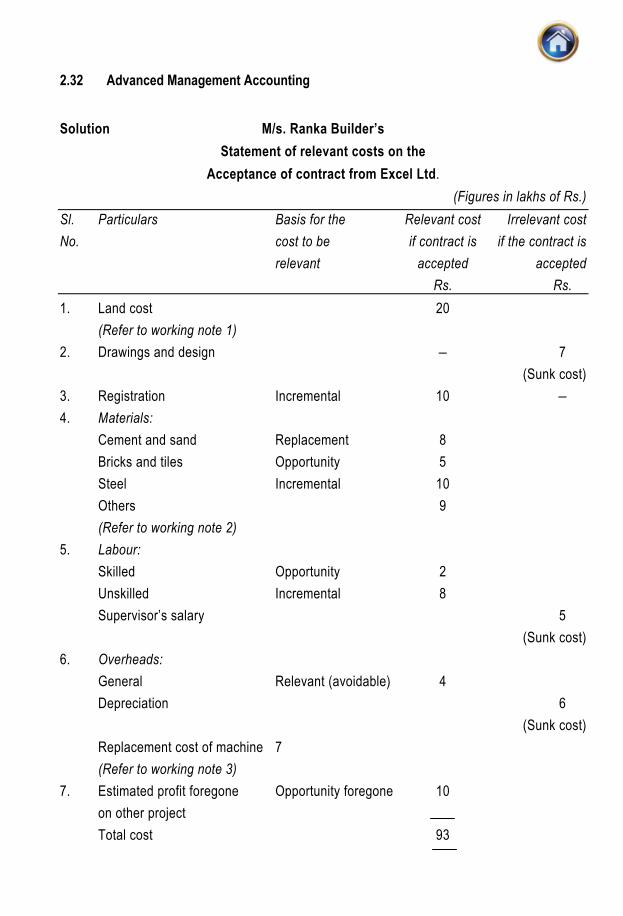
2.32 Advanced Management Accounting
Solution M/s. Ranka Builder’s Statement of relevant costs on the Acceptance of contract from Excel Ltd.
(Figures in lakhs of Rs.) Sl. Particulars Basis for the Relevant cost Irrelevant cost No. cost to be if contract is if the contract is relevant accepted accepted Rs. Rs. 1. Land cost 20 (Refer to working note 1) 2. Drawings and design – 7 (Sunk cost) 3. Registration Incremental 10 – 4. Materials: Cement and sand Replacement 8 Bricks and tiles Opportunity 5 Steel Incremental 10 Others 9 (Refer to working note 2) 5. Labour: Skilled Opportunity 2 Unskilled Incremental 8 Supervisor’s salary 5 (Sunk cost) 6. Overheads: General Relevant (avoidable) 4 Depreciation � 6 (Sunk cost) Replacement cost of machine 7 (Refer to working note 3) 7. Estimated profit foregone Opportunity foregone 10 on other project Total cost 93

Cost Concepts in Decision Making 2.33
Decision: Since the offer price of contract is Rs. 1 crore and its total relevant cost is Rs. 93 lacs; these figures clearly show that the offer should be accepted. Working notes : (Rs.in lakhs)
1. Total cost of 3 grounds of land 60 Cost of 2 grounds of land will be borne by Excel Ltd. 40 Cost of 1 ground of land will be 20 borne by M/s. Ranka Builders 2. Others material cost of Rs. 10 lakhs includes material worth Rs. 2 lakhs relating to
interior decoration, which is a sunk cost, this material can be sold for Rs 1 lac (which is a relevant opportunity cost) and Rs. 8 lakhs material is an incremental cost. Hence total relevant cost of others material is Rs. 9 lakhs (Rs. 8 lakhs incremental + Rs. 1 lac opportunity cost).
3. Since the equipment can also be used on this contract its current replacement price is Rs. 32 lakhs and after one year its cost will be Rs. 25 lacs. Therefore the relevant opportunity cost of machine is : Rs. 7 lakhs {Rs. 32 lakhs � Rs. 25 lacs}.
Illustration : decision on acceptance of a contract Intervero Ltd., a small engineering company, operates a job order costing system. It has been invited to tender for a comparatively large job which is outside the range of its normal activities and, since there is surplus capacity, the management are keen to quote as low a price as possible. It is decided that the opportunity should be treated in isolation without any regard to the possibility of its leading to further work of a similar nature (although such a possibility does exist). A low price will not have repercussions on Intervero’s regular work. The estimating department has spent 100 hours on work in connection with the quotation and they have incurred travelling expense of Rs.550 in connection with a visit to the prospective customers’ factory. The following cost estimates has been prepared on the basis of their study. Inquiry 205 H 81 Cost Estimate (Rs.) (Rs.) Direct material and components: 2,000 units of A at Rs.25 per unit 50,000 200 units of B at Rs.10 per unit 2,000 Other material and components to be bought is (specified) 12,500 64,500

2.34 Advanced Management Accounting
Direct labour: 700 hrs. of skilled labour at Rs.3.50 per hour 2,450 1,500 hrs. of unskilled labour at Rs.2 per hour 3,000 Overhead: Department P- 200 hrs. at Rs.25 per hour 5,000 Department Q- 400 hrs. at Rs.20 per hour 8,000 Estimating Department: 100 hours at Rs.5 per hour 500 Travelling expenses 550 Planning Department: 300 hours at Rs.5 per hour 1,500 85,500 The following information has been brought together: Material A: This is a regular stock item. The stock holding is more than sufficient for this job. The material currently held has an average cost of Rs.25 per unit but the current replacement cost is Rs.20 per unit. Material B: A stock of 4,000 units of B is currently held in the stores. This material is slow moving and the stock is the residue of a batch bought seven years ago at a cost of Rs.10 per unit. B currently costs Rs.24 per unit but the resale value is only Rs.18 per unit. A foreman has pointed out that B could be used as a substitute for another type of regularly used raw material which costs Rs.20 per unit. Direct Labour: The work force is paid on a time basis. The company has adopted no redundancy policies which mean that skilled workers are frequently moved to jobs which do not make proper use of their skills. The wages included in the cost estimate are for the mix of labour which the job ideally requires. It seems likely, if the job is obtained, that most of the 2,200 hours of direct labour will be performed by skilled staff receiving Rs.3.50 per hour. Overhead: Department P : It is a department of Intervero Ltd., that is working at full capacity. The department is treated as a profit centre and it uses a transfer price of Rs.25 per hour for charging out its processing time to other departments. This charge is calculated as follows: Rs. Estimated variable cost per machine hour 10 Fixed departmental overhead 8 Departmental profit 7 25 Department P’s facilities are frequently hired out to other firms and a charge of Rs.30 per hour is made. There is a steady demand from outside customers for the use of these facilities.

Cost Concepts in Decision Making 2.35
Overhead :Department Q : Department Q uses a transfer price of Rs.20 for charging out machine processing time to other Departments. This charge is calculated as follows : Rs. Estimated variable cost per machine hour 8 Fixed departmental overhead 9 Departmental profit 3 20 Estimating department : This department charges out its time to specific jobs using a rate of Rs.5/- per hour. The average wage rate within the department is Rs.2.50 per hour but the higher rate is justified as being necessary to cover departmental overheads and the work done on unsuccessful quotations. Planning department: This department also uses a charging out rate which is intended to cover all departmental costs. The offer received for the above contract is Rs.70,000. You are required to restate the cost estimate by using an opportunity cost approach. Make any assumptions that you deem to be necessary and briefly justify each of the figures that you give. Solution
Statement of cost of Intevero Ltd. Rs. Direct material : A: 2,000 units @ Rs.20 40,000 (Refer to working note 1) B: 200 units @ Rs.20 4,000 (Refer to working note 2) Direct labour (skilled) 12,500 Direct labour (Unskilled) sunk (Refer to working note 3) Overheads: Dept. P: 200 hrs. @ Rs.30 6,000 (Refer to working note 4) Dept. Q: 400 hrs. @ Rs.8 3,200 Estimating department sunk Planning department sunk Total cost 65,700

2.36 Advanced Management Accounting
Working notes: 1. Material A is a regularly used item. Therefore, the present stock is not meant for this
contract. Hence, the replacement cost is considered. 2. Material B will be sold if not used for this contract. Therefore, the resale value (Rs.20 or
Rs. 18 whichever is more should be considered). 3. The entire job will be performed by skilled workers (unskilled jobs also). This implies
skilled workers are idle at present and since the company follows no redundancy policy and their wages will be paid on time basis whether the contract is accepted or not. Hence, they are treated as a sunk cost.
4. Department P is a profit centre and is working at full capacity at present and has a steady demand from outside for its facilities at Rs.30 per hour. Therefore, we should consider this Rs.30\hr. as relevant (out of pocket cost Rs.10 + opportunity cost of Rs.20).
5. Department Q : Only the out of pocket costs being the variable overheads of Rs.8\ hr. should be considered.
6. All other costs mentioned are sunk costs. Conclusion: We should accept this offer.
Illustration : Decision on use of alternative resources B Ltd. is a company that has in stock, materials of type XY that cost Rs. 75,000, but that are now obsolete and have a scrap value of only Rs. 21,000. Other than selling the material for scrap, there are only two alternative uses for them. Alternative 1 – Converting the obsolete materials into a specialised product, which would require the following additional work and materials – Material A 600 units Material B 1,000 units Direct Labour 5,000 hours unskilled 5,000 hours semi-skilled 5,000 hours highly skilled Extra selling and delivery expenses Rs. 27,000 Extra advertising Rs. 18,000 The conversion would produce 900 units of saleable product and these could be sold for Rs. 300 per unit. Material A is already in stock and is widely used within the firm. Although present stocks, together with orders already planned, will be sufficient to facilitate normal activity and extra material used by adopting this alternative will necessitate such materials being replaced

Cost Concepts in Decision Making 2.37
immediately. Material B is also in stock, but it is unlikely that any additional supplies can be obtained for some considerable time because of an industrial dispute. At the present time material B is normally used in the production of product Z, which sells at Rs. 390 per unit and incurs total variable (cost excluding Material B) of Rs. 210 per unit. Each unit of product Z uses four unis of Material B. The details of Materials A and B are as follows : Material A Material B (Rs.) (Rs.) Acquisition cost at the time of purchase 100 per unit Rs. 10 per unit Net realizable value 85 per unit Rs. 18 per unit Replacement cost 90 per unit — Alternative 2 – Adopting the obsolete materials for use as a substitute for a sub-assembly that is regularly used within the firm. Details of the extra work and materials required are as follows: Material C 1,000 units Direct Labour 4,000 hours unskilled 1,000 hours semi-skilled 4,000 hours highly skilled 1,200 units of the sub-assembly are regularly used per quarter at a cost of Rs. 900 per unit. The adaptation of material XY would reduce the quantity of the sub-assembly purchased from outside the firm to 900 units for the next quarter only. However, since the volume purchased would be reduced, some discount would be lost and the price of those purchased from outside would increase to Rs. 1,050 per unit for that quarter. Material C is not available externally though 1,000 units required would be available from stocks, it would be produced as extra production. The standard cost per unit of Material C would be as follows : Rs. Direct labour 6 hours unskilled labour 18 Raw materials 13 Variable overhead : 6 hours at Re. 1 6 Fixed overhead : 6 hours at Rs. 3 18 55 The wage rates and overhead recovery rates for B Ltd are : Variable overhead Re 1 per direct labour hour Fixed overhead Rs 3 per direct labour hour Unskilled labour Rs 3 per direct labour hour

2.38 Advanced Management Accounting
Semi-skilled labour Rs 4 per direct labour hour Highly skilled labour Rs 5 per direct labour hour The unskilled labour is employed on a casual basis and sufficient labour can be acquired to exactly meet the production requirements. Semi-skilled labour is part of the permanent labour force, but the company has temporary excess supply of this type of labour at the present time. Highly skilled labour is in short supply and cannot be increased significantly in the short-term, this labour is presently engaged in meeting the demand for product L, which requires 4 hours of highly skilled labour. The contribution from the sale of one unit of product L is Rs. 24. Given the above information, you are required to present cost information advising whether the stocks of Material XY should be sold, converted into a specialised product (Alternative 1) or adopted for use as a substitute for a sub-assembly (Alternative 2). Solution Alternative 1 – (Conversion versus immediate sale) Rs. Rs. Rs. Sales revenue 900 units at Rs. 300 per unit 2,70,000 (Refer to working note 1) Less : Relevant costs Material XY opportunity cost 21,000 (Refer to working note 2) Material A – 600 units @ Rs. 90 per unit 54,000 (Refer to working note 3) Material B – 1,000 units @ Rs. 45 per unit 45,000 (Refer to working note 4) Direct Labour : Unskilled - 5,000 hours @ Rs. 3 per hour 15,000 Semi-skilled NIL Highly skilled - 5,000 hours @ Rs. 11 55,000 70,000 (Refer to working note 5) Variable overheads 15,000 hours @ Rs. 1 15,000 (Refer to working note 6) Extra selling and delivery expenses 27,000 Extra advertising 18,000 45,000 2,50,000 Fixed overheads NIL (To remain same, not relevant) Excess of relevant revenues 20,000

Cost Concepts in Decision Making 2.39
Alternative 2 – (Adaptation versus immediate sale) Saving on purchase of sub-assembly : Normal spending - 1,200 units @ Rs. 900 per unit 10,80,000 Less : Revised spending - 900 units @ Rs. 1,050 per unit 9,45,000 1,35,000 (Refer to working note 7) Less : Relevant costs Material XY opportunity cost 21,000 (Refer to working note 2) Material C - 1,000 units @ Rs. 37 37,000 (Refer to working note 8) Direct labour Unskilled – 4,000 hours @ Rs. 3 per hour 12,000 Semi-skilled NIL Highly skilled – 4,000 hours @ Rs. 11 per hour 44,000 56,000 (Refer to working note 5) Variable overheads – 9,000 hours @ Re. 1/- per hour 9,000 1,23,000 (Refer to working note 6) Fixed overheads NIL (To remain same not relevant) Net relevant savings 12,000 Evaluation : The evaluation of two alternatives clearly shows that Alternative 1, yields higher net revenue of Rs. 8,000 (Rs. 20,000 – Rs. 12,000). Hence because of higher net revenue of Alternative 1, it is adviseable to convert material XY into a specialised product. Working notes : 1. There will be an additional sales revenue of Rs. 2,70,000 if Alternative 1 is choosen. 2. Acceptance of either Alternative 1 or 2 will mean a loss of revenue of Rs. 21,000 from the
sale of the obsolete material XY and hence it is an opportunity cost for both of the alternatives. The original purchase cost of Rs. 75,000 is a sunk cost and thus not relevant.
3. Acceptance of Alternative 1 will mean that material A must be replaced at an additional cost of Rs. 54,000.

2.40 Advanced Management Accounting
4. Acceptance of Alternative 1 will mean diversion of material B from the production of product Z. The excess of relevant revenues over relevant cost for product Z is Rs. 180 (Rs. 390 – Rs. 210) and each unit of product Z uses four units of material B. The lost contribution (excluding the cost of material B which is incurred for both alternatives) will therefore be Rs. 45 for each unit of material B, that is used for converting the obsolete materials into a specialised product.
5. Unskilled labour can be matched exactly to the company’s production requirements. Hence acceptance of either alternative 1 or 2 will cause the company to incur additional unskilled labour cost at Rs. 3 for each hour. It is assumed that the semi-skilled labour will be able to meet the extra requirements of either alternatives at no extra cost to the company. Hence, cost of semi–skilled labour will not be relevant. Skilled labour is in short supply and can only be obtained by reducing the production of product L, resulting in a loss of contribution of Rs. 24 (given) or Rs. 6 per hour of skilled labour. Hence the relevant labour cost will be Rs. 6 (contribution lost per hour) + Rs. 5 (hourly rate of skilled labour) i.e. Rs. 11 per hour.
6. It is assumed that for each direct labour of input, variable overhead will increase by Re. 1, hence for each alternative using additional direct labour hours, variable overheads will increase.
7. The cost of purchasing the sub-assembly will be reduced by Rs. 1,35,000 if the second alternative is choosen and so these savings are relevant to the decision.
8. The company will incur additional variable costs of Rs. 37 for each unit of material C that is manufactured, so the fixed overheads for material C viz. Rs. 18/- per unit is not a relevant cost.
2.1.4 Sunk costs: Costs which do not change under given circumstance and do not play any role in decision making process are known as sunk costs. They are historical costs incurred in the past. In other words, these are the costs which have been incurred by a decision made in past and cannot be changed by any decision made in the future. Out of pocket costs: This is that portion of costs which involves payments to outsiders i.e., it gives rise to cash expenditure as opposed to such costs as depreciation, which do not involve any cash expenditure. Such costs are relevant for price fixation during recession or when make or buy decisions are to be made. These costs include cost incurred under some heads for which separate cost accounting records are not maintained and they are sometimes termed as misclleneous cost.
2.2 APPLICATION OF INCREMENTAL/DIFFERENTIAL COST TECHNIQUES IN MANAGERIAL DECISIONS:
It is a technique used for arriving at managerial decisions in which only cost and income differences between alternative courses of action are taken into consideration. This technique is applicable to situations where fixed costs alter. This technique emphasizes on comparing the incremental costs with incremental revenues for taking a managerial decision. So long as
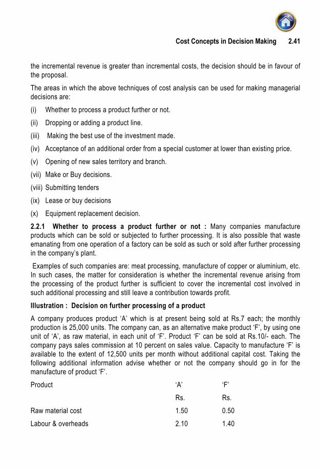
Cost Concepts in Decision Making 2.41
the incremental revenue is greater than incremental costs, the decision should be in favour of the proposal. The areas in which the above techniques of cost analysis can be used for making managerial decisions are: (i) Whether to process a product further or not. (ii) Dropping or adding a product line. (iii) Making the best use of the investment made. (iv) Acceptance of an additional order from a special customer at lower than existing price. (v) Opening of new sales territory and branch. (vii) Make or Buy decisions. (viii) Submitting tenders (ix) Lease or buy decisions (x) Equipment replacement decision. 2.2.1 Whether to process a product further or not : Many companies manufacture products which can be sold or subjected to further processing. It is also possible that waste emanating from one operation of a factory can be sold as such or sold after further processing in the company’s plant. Examples of such companies are: meat processing, manufacture of copper or aluminium, etc. In such cases, the matter for consideration is whether the incremental revenue arising from the processing of the product further is sufficient to cover the incremental cost involved in such additional processing and still leave a contribution towards profit. Illustration : Decision on further processing of a product A company produces product ‘A’ which is at present being sold at Rs.7 each; the monthly production is 25,000 units. The company can, as an alternative make product ‘F’, by using one unit of ‘A’, as raw material, in each unit of ‘F’. Product ‘F’ can be sold at Rs.10/- each. The company pays sales commission at 10 percent on sales value. Capacity to manufacture ‘F’ is available to the extent of 12,500 units per month without additional capital cost. Taking the following additional information advise whether or not the company should go in for the manufacture of product ‘F’. Product ‘A’ ‘F’ Rs. Rs. Raw material cost 1.50 0.50 Labour & overheads 2.10 1.40
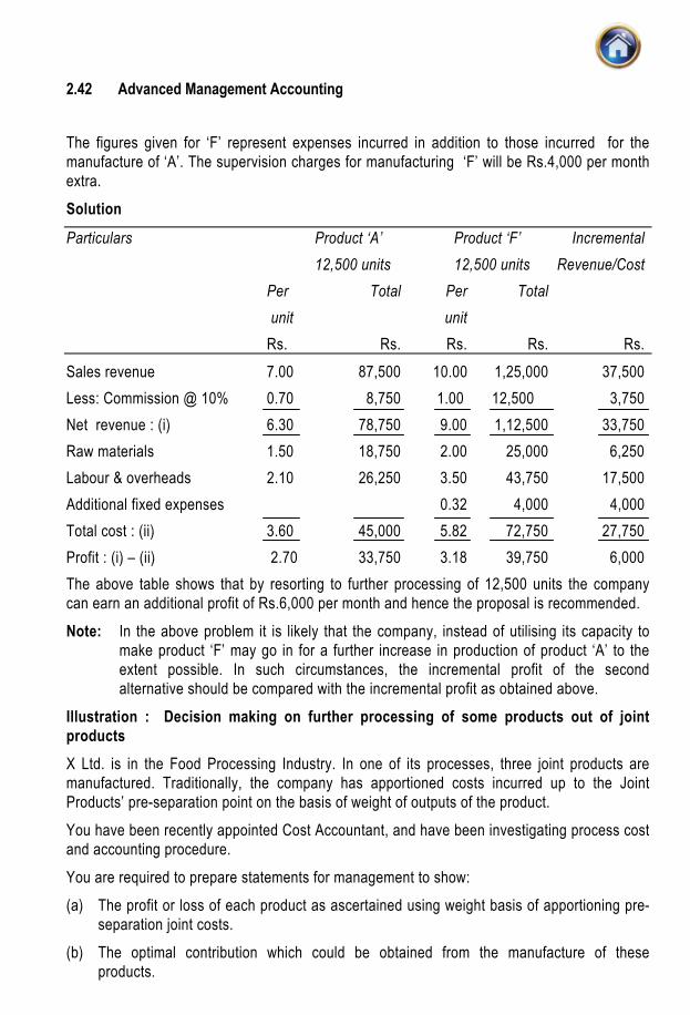
2.42 Advanced Management Accounting
The figures given for ‘F’ represent expenses incurred in addition to those incurred for the manufacture of ‘A’. The supervision charges for manufacturing ‘F’ will be Rs.4,000 per month extra. Solution
Particulars Product ‘A’ Product ‘F’ Incremental 12,500 units 12,500 units Revenue/Cost Per Total Per Total unit unit Rs. Rs. Rs. Rs. Rs. Sales revenue 7.00 87,500 10.00 1,25,000 37,500 Less: Commission @ 10% 0.70 8,750 1.00 12,500 3,750 Net revenue : (i) 6.30 78,750 9.00 1,12,500 33,750 Raw materials 1.50 18,750 2.00 25,000 6,250 Labour & overheads 2.10 26,250 3.50 43,750 17,500 Additional fixed expenses 0.32 4,000 4,000 Total cost : (ii) 3.60 45,000 5.82 72,750 27,750 Profit : (i) – (ii) 2.70 33,750 3.18 39,750 6,000 The above table shows that by resorting to further processing of 12,500 units the company can earn an additional profit of Rs.6,000 per month and hence the proposal is recommended. Note: In the above problem it is likely that the company, instead of utilising its capacity to
make product ‘F’ may go in for a further increase in production of product ‘A’ to the extent possible. In such circumstances, the incremental profit of the second alternative should be compared with the incremental profit as obtained above.
Illustration : Decision making on further processing of some products out of joint products X Ltd. is in the Food Processing Industry. In one of its processes, three joint products are manufactured. Traditionally, the company has apportioned costs incurred up to the Joint Products’ pre-separation point on the basis of weight of outputs of the product. You have been recently appointed Cost Accountant, and have been investigating process cost and accounting procedure. You are required to prepare statements for management to show: (a) The profit or loss of each product as ascertained using weight basis of apportioning pre-
separation joint costs. (b) The optimal contribution which could be obtained from the manufacture of these
products.

Cost Concepts in Decision Making 2.43
The following process data for December are given. Cost incurred up to separation point are Rs.96,000 : Product A Product B Product C Cost incurred after separation point (Rs.) 20,000 12,000 8,000 Selling price per Ton of
completed product (Rs.) 500 800 600 Estimated, if sold at
separation point (Rs.) 250 700 450 Output (Tons) 100 60 80 The cost of any unused capacity after the separation point should be ignored. Solution (a) Statement showing profit or loss of each product using weights as the basis of
apportioning pre-separation joint costs Total Product A Product B Product C Rs. Rs. Rs. Rs. Cost upto the point of separation in the ratio of (100: 60: 80) or (5:3:4) 96,000 40,000 24,000 32,000 Cost after separation point 40,000 20,000 12,000 8,000 Total costs 1,36,000 60,000 36,000 40,000 Sales revenue 1,46,000 50,000 48,000 48,000 Profit/(Loss) 10,000 (10,000) 12,000 8,000 (b) To ascertain optimal contribution, first, the incremental profit or loss from each
product, if products are further processed after separation point is to be computed. The statement below shows the incremental profit or loss after further processing:
Product A Product B Product C
Rs. Rs. Rs. Output (Tons) 100 60 80 Incremental revenue from further processing 25,000 6,000 12,000 (Rs.500–Rs.250)×100 (Rs.800–Rs.700)×60 (Rs.600–Rs.450)×80 Less: Incremental cost 20,000 12,000 8,000 Incremental profit (loss) 5,000 (6,000) 4,000

2.44 Advanced Management Accounting
It will be seen from the above statement that there will be a loss of Rs.6,000 if further processing of product B is done after the separation point. It is, therefore, recommended that Product B should be sold at separation point. The optimal contribution based on this recommendation will be as follows:
Statement showing optimal contribution
Product A Product B Product C Total
Output (Tons) 100 60 80 Rs. Rs. Rs. Rs. Sales revenue 50,000 42,000 48,000 1,40,000 (100×Rs.500) (60×Rs.700) (80×Rs.600) Less: Post separation cost 20,000 — 8,000 28,000 Contribution 30,000 42,000 40,000 1,12,000
2.2.2 Dropping or adding a product line: Often firms manufacturing a number of products may find that one or more of its products are not worthwhile for producing from the profitability point of view. Since the objective of any business organisation is to maximise its profits, the firm can in such cases consider the economies of dropping such unprofitable products, and adding a more profitable product(s). In such cases, the firm may have two alternatives as under: (a) To drop the unprofitable product and to leave the capacity unutilised. (b) To drop the unprofitable product and to utilise the capacity for the manufacture of a more
remunerative product. If we consider alternative (a) above, what is more important is the amount of fixed expenses apportioned to the product which is going to be discontinued. If the capacity relating to the product in question is going to be left unutilised, the contribution which the product is making towards recovery of fixed expenses will not be forthcoming. Thus continuance of a product line which is adjudged asunprofitable, on the basis of absorption costing may make matters worse. The use of contribution approach will help the firm to take a sound decision on such occasions. As some of the fixed expenses can be reduced by dropping a product line, such fixed costs become relevant while making a decision about the discontinuance of product line. If we take alternative (b) the fixed expenses apportioned to the product line discontinued will remain the same for being absorbed by the new product. The comparison is now between discontinuance of the product line and introduction of another remunerative product line. Since the fixed expenses are not going to be reduced in this alternative, the product which yields the highest contribution is preferred because it will maximise the overall profitability of the firm.

Cost Concepts in Decision Making 2.45
Illustration : Adding a new product lines A firm produces three products, the details of sales, contribution margin and the fixed costs apportioned to the products are as under:
Products A B C Sales values (Rs.) 10,00,000 8,00,000 2,00,000 Contribution (Rs.) 40% 30% 25% Fixed expenses (Rs.) 3,40,000 1,80,000 90,000 Fixed expenses attributable to product ‘C’ are Rs.40,000. Product C incurs a loss and hence the management wishes to consider two alternatives: (i) Discontinue product ‘C’ to save the loss. (ii) Discontinue product ‘C’ and utilise the capacity to manufacture product ‘D’. In this case
the sales value of product D is Rs.2,00,000 and the contribution is 35%. Which alternative should be adopted? Solution (i) Let us tabulate the results of the firm as under: Profitability of the firm: Products A B C Total Sales value (Rs.) 10,00,000 8,00,000 2,00,000 20,00,000 Contribution (%) 40% 30% 25% 34.5%* Contribution (Rs.) 4,00,000 2,40,000 50,000 6,90,000 Fixed costs (Rs.) 3,40,000 1,80,000 90,000 6,10,000 Net profit (loss) (Rs.) 60,000 60,000 (40,000) 80,000 *Rs. 6,90,000
x 100 = 34.5% Average
Rs. 20,00,000
Under alternative (i), a comparison between the total profitability and the profitability without product ‘C’ is relevant, shown as under: Particulars Products Products Difference A,B &C A&B only Sales value (Rs.) 20,00,000 18,00,000 2,00,000 Contribution (Rs.) 6,90,000 6,40,000 50,000 Fixed expenses (Rs.) 6,10,000 5,70,000 40,000 Net profit (Rs.) 80,000 70,000 10,000

2.46 Advanced Management Accounting
It may be observed from the above table that discontinuance of product ‘C’ reduced the total profit from Rs.80,000 to Rs.70,000. In other words, product ‘C’ was yielding a contribution sufficient to cover more than the incremental fixed costs of Rs.40,000 attributable to its manufacture. (ii) Under alternative (ii), comparison between the profitability of product ‘C’ and product ‘D’
is relevant as under:
Particulars Product’C’ Product’D’ Difference Sales value (Rs.) 2,00,000 2,00,000 _ Contribution (%) 25% 35% Contribution (Rs.) 50,000 70,000 20,000
Since product D yields a higher contribution, the total profitability will increase by Rs.20,000. The fixed expenses remain constant. This is illustrated below:
Product A B D Total Sales value (Rs.) 10,00,000 8,00,000 2,00,000 20,00,000 (%) 40% 30% 35% 35.5%* Contribution (Rs.) 4,00,000 2,40,000 70,000 7,10,000 Fixed expenses (Rs.) 3,40,000 1,80,000 90,000 6,10,000 Net profit (loss) (Rs.) 60,000 60,000 (20,000) 1,00,000
*Rs.7,10,000Rs.20,00,000
100 35.5% Average× =
Illustration : Optimization of profit under a limiting factor condition Something More Ltd. is considering adding products to its product line. After a lot of deliberations between the sales and production personnel, it is decided that Products P, Q and R would be the most desirable additions to the company’s product range on account of the technical competency, marketing potential and production flexibility as regards these products. In fact P, Q and R can all be made on the same kind of plant as that already in use and therefore as regards production, all products can be readily interchanged. However, it is considered necessary to build further plant facilities to cater for this additional production.

Solution Something More Ltd.
Statement showing the production of R, Q and P in order of priority determined on the basis of contribution per machine hour, to maximise the profit at various levels of activity
P Q R
(Max. demand = 200 units
Machine hours for max. demand = 3,000 hours)
(Max. demand = 125 units
Machine hours For max. demand
= 62.5 hours)
(Max. demand = 750 units
Machine hours For max demand = 2,250 hours)
Product Levels of Activity
(Machine Hours)
Units Contribution Units Contribution Units Contribution
Total Contribution
Fixed Cost
Net Profit
Rs. Rs. Rs. Rs. Rs. Rs.
1,800 – – – – 600 54,000 54,000 15,000 39,000
2,300 – – 10 1,000 750 67,500 68,500 20,000 48,500
2,800 – – 110 11,000 750 67,500 78,500 26,000 52,5003,300 28* 4,200 125 12,500 750 67,500 84,200 33,000 51,200
3,800 61* 9,150 125 12,500 750 67,500 89,150 39,000 50,150
* 28 and 61 units of product P consumes 420 and 915 machine hours respectively whereas actually 425 and 925 machine hours are available. As incomplete units can be sold only in the next period after they are completed, for these computations only complete units have been considered. The most desirable level of activity to be pursued is at 2,800 machine hours to produce and sell 750 units of R and 110 units of Q. At this activity level profit is maximum, i.e. Rs. 52,500. In this connection the following data are relevant:
Products P Q R Rs. Rs. Rs. Direct materials per unit 100 120 90 Direct labour per unit 50 70 90 Variable overheads per unit 50 130 100 Selling price per unit 350 420 370 Demand in units per cost period 200 125 750 (on the basis of the above selling price) Machine hours required per unit of production 15 5 3

2.48 Advanced Management Accounting
It is felt that initially extra plant facilities can be built to operate at the following five different levels of activity viz. 1,800, 2,300, 2,800, 3,300 and 3,800 machines hours per cost period. The fixed overhead costs for a cost period relevant to these five different levels of activity are estimated at Rs.15,000, Rs.20,000, Rs.26,000, Rs.33,000 and Rs.39,000 respectively. You are required to advise, with supporting figures, the product or products to be manufactured and in what quantities at each of the five contemplated levels of activity that would seem most desirable to be pursued for maximisation of profits. Working note
Computation of contribution per unit of product and per machine hour
Products
P Q R
Rs. Rs. Rs.
Selling price: (A) 350 420 370 Less : Variable costs Direct materials 100 120 90 Direct labour 50 70 90 Variable overheads 50 130 100 Total variable costs: (B) 200 320 280 Contribution per unit: (A–B) 150 100 90 Machine hours required per unit 15 5 3 Contribution per machine hour 10 20 30
For maximizing profits, the products giving the maximum contribution per machine hour should be concentrated upon as machine hours available are the foremost constraint. Hence the order of priority for producing the product should be R, Q, and P. 2.2.3 Optimising Investment plan The investment decisions, also termed as capital budgeting decisions involve current outlays in return for a stream of benefits in future year. When multiple alternatives of investment opportunities having similar risks are available, we can use incremental cost and revenue approach to find out the optimum investment plan. In this case we increase the total investment by increment till such time the incremental rate of return falls below the cut off rate given. The cut off rate is defined as the minimum rate of return expected from the investment.

Cost Concepts in Decision Making 2.49
Illustration : optimization of Investment plan A company has Rs.2,00,000 to invest and it can earn 14% by investing the sum in company deposits. It also has got an opportunity to invest this sum in five projects as under :
Projects A B C D E Rs. Rs. Rs. Rs. Rs. Total investment 20,000 60,000 1,00,000 1,60,000 2,00,000 Annual net profit 1,000 8,400 15,600 24,240 28,640 Rate of return 5% 14% 15.6% 15.15% 14.3% Find the optimum investment plan. Solution The optimum investment plan by using the incremental approach is as under:
Projects B C D E Rs. Rs. Rs. Rs. Incremental investment 40,000 40,000 60,000 40,000 Incremental net profit 7,400 7,200 8,640 4,400 Rate of return on incremental investment 18.5% 18% 14.4% 11.0% Looking at the figures above, we find that project D is the most profitable one because if we take project E, the rate of return on the incremental investment will fall below the cut off rate of 14% and hence not acceptable. The following table will prove the facts. It may be observed here that the total income is the highest figure if the funds are invested in project D and the balance available in other company deposits at 14%.
Project A B C D E Rs. Rs. Rs. Rs. Rs. Total funds available 2,00,000 2,00,000 2,00,000 2,00,000 2,00,000 Funds invested in project 20,000 60,000 1,00,000 1,60,000 2,00,000 Balance invested in deposits 1,80,000 1,40.000 1,00,000 40,000 — Income from project 1,000 8,400 15,600 24,240 28,640 Income from deposits @ 14% 25,200 19,600 14,000 5,600 — Total income 26,200 28,000 29,600 29,840 28,640

2.50 Advanced Management Accounting
Cash flow technique : This technique is useful in making decision regarding investment alternatives. In this technique of decision making only differential cash flows are considered. Cash flow refers to the actual movement of cash in and out of an organisation. When cash is received it is called ‘cash inflows’ or positive cash flow, and when cash is paid out, it is called ‘cash outflows’ or negative cash flow. The difference between the two flows is termed as the net cash flow’. This technique of decision making can be applied in those circumstances in which the prime differences can be measured in terms of the future cash flows of the various alternatives under consideration. An alternative which gives most favourable net cash flow is selected. The application of the cash flow technique involves the following steps: (i) Compute the future cash inflows and the future cash outflows of each alternative under
consideration. (ii) Ascertain the overall net cash flow. (iii) Select the alternative that has the most favourable net cash flow i.e. the highest net cash
flow. Illustration : Make or Buy decision A firm needs component in an assembly operation. If it wants to do the manufacturing itself, it would need to buy a machine for Rs. 4 lakhs which will last for 4 years with no salvage value. Manufacturing costs in each of the 4 years would be Rs. 6 lakhs, Rs. 7 lakhs, Rs. 8 lakhs, and Rs. 10 lakhs respectively. If the firm had to buy the components from a supplier, the cost would be Rs. 9 lakhs, Rs. 10 lakhs, Rs. 11 lakhs and Rs. 14 lakhs respectively in each of the four years. However, the machine would occupy floor space which would have been used for another machine. This latter machine would be hired at no cost to manufacture an item, the sale of which would produce net cash flows in each of the four years of Rs. 2 lakhs. It is impossible to find room for both the machines and there are no other external effects. The cost of capital is 10% and the present value factor for each of the four years is 0.909, 0.826, 0.751 and 0.683 respectively. Should the firm make the components or buy from outside?

Cost Concepts in Decision Making 2.51
Solution Evaluation of Make or Buy proposal (All figures are in lakhs of rupees)
Year P.V. factors When the component When the component at 10% is manufactured is bought from an outside supplier Cash outflow Present Cash outflow Present (Capital cost + value (Buying cost) value manufacturing cost + opportunity cost) Rs. Rs. Rs. Rs (a) (b) (c) (d) = (b) × (c) (e) (f) = (b) × (e) 0 1.000 4 4.000 — — 1 0.909 6+2 7.272 9 8.181 2 0.826 7+2 7.434 10 8.260 3 0.751 8+2 7.510 11 8.261 4 0.683 10+2 8.196 14 9.562 Total 34.412 34.264
= Rs. 34.412 – Rs. 34.264 = Rs. 0.148 (lakhs) Conclusion : Since there is a saving of Rs. 0.148 (lakhs) in buying the component from outside, therefore, we should stick to this decision. Note: The loss of Rs. 2 lakhs cash inflow for each of the four years due to the inability of the
firm to operate another machine if it manufactures the component has been treated as an opportunity cost.
Illustration : decision on alternative channel of sales An item of finished goods inventory that cost Rs.200 per unit to make is facing the danger of becoming obsolete. There are two following alternative ways of disposing it of:

2.52 Advanced Management Accounting
Sell the stock to P for Rs.200; or to Q for Rs.216. Q’s place is twice as far away as that of P though due to favourable transport conditions the delivery time will be the same. The cost accountant has prescribed the following cost estimates for delivery: P - Petrol and oil Rs.10, wages Rs.12, share of licence, insurance and depreciation
(based on mileage) Rs.14. Q - Petrol and oil Rs.20, wages Rs.12, share of licence, insurance and depreciation
Rs.28. You are required to recommend whether the stock should be sold to P or Q. Solution P Q Rs. Rs. Cash inflow (Sales) 200 216 Cash outflow (Petrol, oil and wages) 22 32 Net cash flow 178 184 Since the most favourable net cash flow occurs in the case of sale to Q, hence it is recommended that the item be sold to Q. Notes: 1. In the above analysis Rs.14 and Rs.28 the share of licence, insurance and
depreciation have not been included because there is no actual cash outflow in respect of these costs. Otherwise also these costs are not going to affect the cashflow whether sale is made to P or Q or even to neither of them.
2. It may be noted that the net cashflow does not measure the profits of the projects. It only indicates which project is more profitable.
Note: Students should note that the discounted cash flow technique has been discussed in detail in the book of Management Accounting and Financial Analysis. Students should refer to the aforesaid book to refresh their knowledge.
Illustration : Decision making on the basis of relevant osts CARCARE CORPORATION has just today paid for and installed a special machine for polishing cars at one of its prestigious outlets. It is the first day of company’s fiscal year. The machine costs Rs. 20,000. Its annual operating costs total Rs. 15,000 exclusive of depreciation. The machine will have a four year useful life and a zero terminal disposal value. After the machine has been used for one day, a machine salesman walks in. He offers a different machine that promises to do the same job at a yearly operating cost of Rs. 9,000, exclusive of depreciation. The new machine will cost Rs. 24,000 in cash, duly installed. The “old” machine is unique and can be sold outright for only Rs. 10,000 minus Rs. 2,000 removal cost. The new machine, like the old one, will have a four-year useful life and zero terminal disposal velue.

Cost Concepts in Decision Making 2.53
Sales, all in cash, will be Rs. 1,50,000 annually and other cash costs will be Rs. 1,10,000 annually, regardless of this decision. For simplicity, ignore income taxes, interest and present value considerations. Required : (a) Prepare a statement of cash receipts and disbursements for each of the four years under
both alternatives. What is the cumulative difference in cash flows for the four years taken together ?
(b) Prepare Income Statements for each of the four years under both alternatives. Assume straight-line depreciation. What is the cumulative difference in operating income for the four years taken together ?
(c) What are the irrelevant items in your presentations in requirements (a) and (b) ? Why are they irrelevant ?
(d) Suppose the cost of the “old” machine was Rs. 10,00,000 rather than Rs. 20,000. Nevertheless, the old machine can be sold outright for only Rs. 10,000 minus Rs. 2,000 removal cost. Would the net differences in requirements (a) and (b) change ? Explain.
(e) “To avoid a loss, we should keep the old machine.” What is the role of book value in decisions about replacement of machines ?
Solution (a) Statement of Cash Receipts, Disbursements and cumulative difference in Cash
flows for four years taken together under both alternatives. (Rs. in thousands)
Alternatives Keep old machine Buy new machine Year 1 2nd, 3rd All 4 Year 1 2nd, 3rd All 4 Cumulative & 4th years & 4th yearsdifference in year year cash flows each each for four years taken together Receipts : Sales revenue 150 150 600 150 150 600 Sales of old equipment — — — 8 — 8 Total receipts : (A) 150 150 600 158 150 608 Disbursements : Annual operating cost 15 15 60 9 9 36 Other cash costs 110 110 440 110 110 440

2.54 Advanced Management Accounting
Purchase cost of “old” machine 20 — 20 20 — 20 Purchase of “new” machine — — — 24 — 24 Total disbursements : (B) 145 125 520 163 119 520 Net cash in-flows : (A) – (B) 5 25 80 (5) 31 88 08 (b) Statement of income for each of the four years and cumulative difference in
operating income (Rs. in thousands)
Alternatives Keep old machine Buy new machine Ist, 2nd All 4 Year 1 2nd, 3rd All 4 Cumulative 3rd & 4th years & 4th yearsdifference in year each year each operating Rs. Rs. Rs. Rs. Rs. income Income : Sales revenue 150 600 150 150 600 Total revenue : (A) 150 600 150 150 600 Costs : Annual operating cost 15 60 9 9 36 Other cash costs 110 440 110 110 440 Depreciation 5 20 6 6 24 (Refer to working note 1) Loss on the disposal of old machine — — 12 — 12 (Refer to working note 2) Total costs : (B) 130 520 137 125 512 Operating income : (A) – (B) 20 80 13 25 88 08 (c) The purchase of cost old machine Rs. 20,000; the sales revenue Rs. 1,50,000 and other
cash costs of Rs. 1,10,000 are irrelevant items for the presentation in requirements (a) and (b) above. These items are irrelevant because their amount are common to both the alternatives.
(d) The net difference in requirements under (a) and (b) will not change if the cost of ‘old’ machine becomes Rs. 10,00,000 instead of Rs. 20,000. This is so because the cost of old machine is common for both the alternatives.
(e) In the decision about the replacement of machine the book value of the machine is irrelevant because it is a past (historical) cost. All past costs are down the drain. Nothing can change

Cost Concepts in Decision Making 2.55
what has already happened. As apparent from (a) and (b) above; we can completely ignore the cost of old machine i.e. Rs. 20,000 and still have a correct analysis.
Working Note : 1. Depreciation (according to straight line method) : Old machine New machine (i) Cost of machine (Rs.) 20,000 24,000 (ii) Terminal disposal value (Rs.) Zero Zero (iii) Useful life 4 4
Depreciation
−
)iii()ii()i( Rs. 5,000 6,000
2. Loss on the disposal of old mahcine : Rs. Rs. Purchase price of old machine 20,000 Disposal value 10,000 Less : Removal cost 2,000 8,000 Loss 12,000
SUMMARY • For the purpose of decision making and control, costs are distinguished on the basis of
their relevance to the different type of decisions. • Relevant Costs. : These are the estimated future costs that are different under
alternative courses of action for a specific problem and hence are appropriate to a specific management decision.
• Conditions to be satisfied for relevant costs :- Occur in the Future-every decision deals with selecting a course of action
based on its expected future results. Differ among the alternative courses of action- costs and revenues that do not
differ will not matter and will have no bearing on the decision being made. • Differential cost: Difference in total cost that will arise from the selection of one
alternative instead of another. • Opportunity Cost: Value of the next best alternative. • Sunk Cost: Cost which do not change under given circumstance and do not play any
role in decision making process. • Out Of Pocket Costs : Portion of costs which involves payments to outsiders i.e., it
gives rise to cash expenditure as opposed to other costs such as depreciation, which do not involve any cash expenditure.
• The investment decisions involve current outlays in return for a stream of benefits in future year.
• The cut off rate is defined as the minimum rate of return expected from the investment.

2.56 Advanced Management Accounting
SELF-EXAMINATION QUESTIONS 1. State whether the following statements are true or false:
(a) The essence of management process is decision making. (b) Decision making is one man’s job. (c) While making decision, only relevant cost are considered. (d) Past costs are relevant to the decision at hand. (e) Book value of an old equipment is not relevant to the proposal of equipment
replacement. 2. Fill in the blanks:
(a) The aim of the decision maker is to choose the best out of————courses of action ____________________________________.
(b) Historical costs are ——to decision making. (c) Fixed expenses are relevant to decision at hand only if they are expected to be ——
— by the decision. (d) In a proposal of equipment replacement ——value of old equipment and ——value
of new equipment are relevant. 3. Fill in the blanks: (a) Incremental revenue is the -———— in the total income resulting from a decision. (b) The minimum rate of return expected from an investment is known as —— rate. (c) The opportunity cost of utilising a machine to produce a new product is the
————— that would have been possible by other existing products. (d) The time adjusted rate of return is that rate of discount at which the sum of the ——
— present value is equal to the sum of the ——— present values. 4. State which of the following statements are true or false :
(a) Incremental cost concept can be used for finding an optimum investment plan. (b) Net present value method cannot be used for selecting a capital project. (c) The opportunity cost of a firm’s funds is the interest rate at which banks accept
deposits from the firms. 5. Given the following data which of the answer is correct?
(a) A company’s scrap can be sold at Rs.2/- per kg. After processing at a cost of Rs.1.50, it can be sold at Rs.4/- per kg. Answers : (i) Sell the scrap and do not process further and sell
(ii) Process the scrap further and sell. (b) The net present value of Rs.1,000 received after 3 years at an interest rate of 20%
is: Answers : (i) Rs.712/- (ii) Rs.769/-

Cost Concepts in Decision Making 2.57
6. Following are two types of statements one having questions and the other giving the answers. Connect up the questions with their correct answers:
Questions Answers (a) What is differential cost? (i) It is minimum rate of return expected from an
investment. (b) What is a cut off rate? (ii) It is the rate of discount at which discounted
cash inflows equal discounted cash outflows. (c) What is the internal rate (iii) Excess of discounted cash inf lows over of return? discounted cash outflows. (d) What is net present value (iv) Prospective change in cost following the
adoption of an alternative machine or process. 7. “Costs may be classified in a variety of ways according to their nature and the
information needs of the management..” 8. What is cost analysis? How it is useful in decision making? 9. What is meant by incremental revenue? 10. Indicate the major areas of decision in which differential cost analysis is useful. 11. Write short notes on:
(i) Relevant cost (ii) Opportunity cost (iii) Incremental cost (iv) Sunk cost
12. Gemini Enterprises currently makes as many units of part No. X - 248 as it needs. Sen, General Manager of Gemini Enterprises, has received a quotation from another company for making part no.X-248. Zedco will supply 1,000 units of part No.X-248 per year at Rs.50 per unit. Zedco can begin supply on 1st July, 1998 and continue for 5 years, after which Gemini will not need the part. Zedco can accommodate any change in Gemini’s demand for the part and will supply it for Rs.50 regardless of quantity. Shah, the Controller of Gemini Enterprises, reports the following costs for manufacturing 1,000 units of part No.X-248.
Rs. Direct materials 22,000 Direct labour 11,000 Variable manufacturing overhead 7,000 Depreciation on machine 10,000 Product and process engineering 4,000

2.58 Advanced Management Accounting
Rent 2,000 Allocation of general plant overhead costs 5,000 Total costs 61,000
The following additional information is available:
(a) Part X-248 is made on a machine used exclusively for its manufacture. The machine was acquired on 1st July, 1997 at a cost of Rs.60,000. The machine has a useful life of six years and a zero terminal disposal price. Depreciation is calculated on straight-line basis.
(b) The machine could be sold today for Rs.15,000. (c) Product and process engineering costs are incurred to ensure that the manufacturing
process for part No.X-248 works smoothly. Although these costs are fixed in the short run, with respect to units of part No. X-248, they can be saved in the long run if part no.X-248 is no longer produced. If part no. X-248 is outsourced, product and process engineering costs of Rs.4,000 will be incurred for 1997-98 but not thereafter.
(d) Rent costs of Rs.2,000 are allocated to products on the basis of the floor space used for manufacturing the product. If part number X-248 is discontinued, the space currently used to manufacture it would become available. The company could then use the space for storage purposes and saves Rs.1,000 currently paid for outside storage.
(e) General plant overhead costs are allocated to each department on the basis of direct manufacturing labour costs. The costs will not change in total. But no general plant overhead will be allocated to part number X-248 if the part is outsourced.
Assume that Gemini requires a 12% rate of return for this project. The following information may be useful:
Year Present Value Factor at 12% 0 1.000 1 0.893 2 0.797 3 0.712 4 0.636 5 0.567 Required : (i) Should part number X-248 be outsourced ? Prepare a quantitative analysis. (ii) State any sensitivity analysis that seems to be advisable. Do not perform any sensitivity
calculations. (iii) Sen is particularly concerned about his bonus for 1997-98. The bonus is based on the
accounting income of Gemini Enterprises. What decision will Sen make if he wants to maximise his bonus for 1997-98?

Cost Concepts in Decision Making 2.59
13. Mahila Griha Udyog Industries is considering to supply its products - a special range of namkeens-to a departmental store. The contract will last for 50 weeks, and the details are given below:
Rs. Material : X (in stock - at original cost) 1,50,000 Y (on order - on contract) 1,80,000 Z (to be ordered) 3,00,000 Labour : Skilled 5,40,000 Non-skilled 3,00,000 Supervisory 1,00,000 General overheads 10,80,000 Total cost 26,50,000 Price offered by department store 18,00,000 Net Loss 8,50,000 Should the contract be accepted if the following additional information is considered? (i) Material X is an obsolete material. It can only be used on another product, the material
for which is available at Rs.1,35,000 (Material X requires some adaptation to be used and costs Rs.27,000).
(ii) Material Y is ordered for some other product which is no longer required. It now has a residual value of Rs.2,10,000.
(iii) Skilled labour can work on other contracts which are presently operated by semi-skilled labour at a cost of Rs.5,70,000.
(iv) Non-skilled labour are specifically employed for this contract. (v) Supervisory staff will remain whether or not the contract is accepted. Only two of them
can replace other positions where the salary is Rs.35,000. (vi) Overheads are charged at 200% of skilled labour. Only Rs.1,25,000 would be avoidable,
if the contract is not accepted. ANSWERS TO SELF EXAMINATION QUESTIONS
1. (a) True (b) False (c) True (d) False (e) True 2. (a) alternative, (b) irrelevant, (c) altered, (d) disposal, book. 3. (a) Change, (b) cut off, (c) earnings (d) positive, negative. foregone,

2.60 Advanced Management Accounting
4. (a) True, (b) False, (c) Not true in all cases. 5. (a) Process the scrap further and sell; (b) Rs.712 6. (a) with (iv); (b) with (i); (c) with (ii); (d) with (iii) 12. (i) Since the outsourcing has negative NPV, therefore part should continue to be made
internally. (ii) As the outsourcing will start from July 1998, the bonus which Mr. Sen expect will
remain the same. 13. The net benefit on accepting the contract is Rs. 1,52,000 therefore the contact should be
accepted.

3 CVP Analysis and Decision making
LEARNING OBJECTIVES : After studying this unit you will be able to : • Understand meaning and theory of Marginal Costing. • Explain difference between Marginal Costing and Absorption Costing. • Understand method of computing breakeven point in terms of units and sale value. • Understand meaning of margin of safety and its computation. • Calculate and interpret contribution to sales ratio. • Understand method of drawing a conventional breakeven chart • Understand advantages of a contribution breakeven chart and how to draw and use it. • Understand advantages of a profit volume chart and the method of drawing and using it. • Understand limitations of breakeven analysis. • Calculate breakeven points for multipurpose situations
3.1 INTRODUCTION According to CIMA, Marginal costing is the sysem in which variable costs are charged to cost units and fixed costs of the period are written off in full against the aggregate contribution. Marginal costing is not a distinct method of costing like job costing, process costing, operating costing, etc. but a special technique used for marginal decision making. Marginal costing is used to provide a basis for the interpretation of cost data to measure the profitability of different products, processes and cost centre in the course of decision making. It can, therefore, be used in conjunction with the different methods of costing such as job costing, process costing, etc., or even with other technique such as standard costing or budgetary control. In marginal costing, cost ascertainment in made on the basis of the nature of cost. It gives consideration to behaviour of costs. In other words, the technique has developed from a particular concept and expression of the nature and behaviour of costs and their effect upon the profitability of an undertaking.

Advanced Management Accounting 3.2
Cost-volume-profit analysis (as the name suggests) is the analysis of three variable viz., cost, volume and profit. Such an analysis explores the relationship existing amongst costs, revenue, activity levels and the resulting profit. It aims at measuring variations of cost with volume. In the profit planning of a business, cost-volume-profit (C-V-P) relationship is the most significant factor. The CVP analysis is an extension of marginal costing. It makes use of principles of marginal costing. It is an important tool of planning. It is quite useful in making short run decisions. For this purpose we apply the concept of Marginal Costing. Following definitions are required for this purpose 1. Profit Statement Under Marginal Costing Statement of Profit Rs. Rs. Revenue/Sales xxx Less : Variable cost of production Material xx Labour xx D. Expenses xx Variable overhead xx xx Add : Opening Finished goods (at MC) xx Less : Closing Finished goods (at MC) xx Variable cost of goods sold xxx Add: Variable Selling overhead xx Variable cost of sales ×× Contribution xx Less : All types of Fixed cost _xx ( Committed, Discretionary steps ) xx 2. Sales - Variable Cost = Contribution = Fixed Cost + Profit
3. P/V ratio (or C/S ratio) = Contribution ÷ Sales
= Contribution per unit ÷ Selling price per unit
= Change in Contribution ÷ Change in Sales

CVP Analysis and Decision Making 3.3
4. Break-even Point : Point where there is no profit or no loss. i) at BEP, Contribution = Fixed Cost Thus, Break Even Sales ( in sales value ) = Fixed Cost ÷ P/V ratio 5. Margin of safety = Sales – BEP sales = Contribution / P/V ratio - Fixed cost / P/V ratio = Profit / P/V ratio 6. Profit = (Sales × P/V ratio) – Fixed Cost = (Margin of Safety Sales) × P/V ratio 7. BEP Calculation in different scenario : (i) With out limiting factor ( non- attributable to a single product ) BEP in units = Fixed cost ÷ Average contribution p.u. (when sales mix in units are given ) BEP in Rs. = Fixed cost ÷ composite p\v ratio (when sales mix in rupee are given ) where composite p\v ratio = ÷ [ Sales Mix ÷ P\V Ratio ] (ii) With limiting factor ( attributable to a single product ) Find contribution per limiting factor & give rank . Find total contribution from 1st rank
product . Calculate the amount of fixed cost still to recover. Whether it can be recovered by 2nd rank product or not ?
(iii) For Perishable product apply the same concept in case of opening stock with different variable cost.
e. BEP in case of process costing is expressed in terms of total raw material input f. In capital budgeting , BEP is that sales volume where Sdiscounted Cash in flow =
Sdiscounted Cash out flow. In case of perpetuity , the financing charge p.a.= CIF pa g. Potential BE : On the basis of sales out of current period production only. h. Multiple BE : Different BE due to change in sales price, variable costs & fixed
costs for different production level. i. Cash BEP = Cash fixed cost ¸ contribution p.u. So do not consider the sunk cost. j. BEP for decision making purpose : Accept that proposal where BEP is lowest
provided the profit can not be calculated.
3.2 IMPORTANT FACTORS IN MARGINAL COSTING DECISIONS In all recommendations of marginal costing decisions, the following factors are to be considered: (i) Whether the product or production line in question makes a contribution.

Advanced Management Accounting 3.4
(ii) Where a choice is to be made between two courses of action, the additional fixed overhead, if any, should be taken into account.
(iii) The continuity of demand after expansion or renovation or installation of the sophisticated machine and its impact on the selling price should also be considered. For example, if the selling price goes down when the supply increases the possible drop in profit should be taken into account.
(iv) Cost is not the only criterion for decision making. Non-cost factors like the necessity to retain the experienced employees, etc. should also be considered.
3.3 PRICING DECISIONS UNDER SPECIAL CIRCUMSTANCES If goods were sold in the normal circumstances under normal business conditions, the price would cover the total cost plus a margin of profit. Selling prices are not always determined by the cost of production. They may be determined by market conditions but in the long run they tend to become equal to the cost of production of marginal firm. Therefore, a business cannot continue to sell below the total cost for a long period. Occasionally, a firm may have to sell below the total cost. The problem of pricing can be summarised under three heads: (i) Pricing in periods of recession, (ii) Differential selling prices, and (iii) Acceptance of an offer and submission of a tender. 3.3.1 Pricing in periods of recession : In periods of recession, a firm may sell its articles at a price less than the total cost but above the marginal cost for a limited period. The advantages of this practice are: (i) The firm can continue to produce and use the services of skilled employees who are well
trained and will be difficult to re-employ later if discharged. (ii) Plant and machinery can be prevented from deterioration through idleness. (iii) The business would be ready to take advantage of improved business conditions later. (iv) This avoids the competition of securing the business of the firm. One thing to remember here is that a situation like this should not lead to a drastic price cutting and the orders accepted should not cover a long period extending over the production facilities of a period when business conditions improve. It may also be justifiable to sell the product at a price below marginal cost for a limited period provided the following conditions prevail: (i) Where materials are of perishable nature. (ii) Where stocks have been accumulated in large quantities and the market prices have
fallen. This will save the carrying cost of stocks.

CVP Analysis and Decision Making 3.5
(iii) Is it essential to reduce the prices to such an extent in order to popularise a new product?
(iv) Where such reduction enables the firm to boost the sales of other products having larger profit margin.
3.3.2 Differential selling prices : Use of differential selling price which is above, the marginal cost but below the total cost is resorted to in order to absorb surplus capacity. There are two ways of doing this: (i) The firm producing a branded article may use the surplus capacity to produce the same
article to be sold above marginal cost in a different market. Dumping of goods in the export market is an example of this type of pricing. The articles sold in the home market will recover all fixed expenses. Since price
reduction in the home market is injurious to the normal sales, it is not resorted to. Any reduction in the selling prices in the export market will not affect the price prevailing in the home market.
(ii) The firm may produce and sell a branded article, say product A, which covers the entire fixed overheads and use the surplus capacity to produce another product B, which may be sold at a price above its marginal cost. The overall profitability will thus increase. The manufacture of product B, however, should be confined to surplus capacity and it should not have the possibility of becoming a major product at the low price at which it is sold. If it becomes so there will be a reduction in profit as illustrated below :
Example
Condition 1 Condition 2 Product A Product B Product A Product B
Capacity 90% 10% 60% 40% Sales 9,000 2,000 6,000 8,000 Marginal cost 6,000 1,800 4,000 7,200 Gross margin 3,000 200 2,000 800 Fixed expenses 2,000 — 2,000 — Profit 1,000 200 — 800
Total profit 1,200 800
Surplus capacity is assumed to be 10% in the above example. 3.3.3 Acceptance of an offer and submission of a tender Acceptance of an offer : When a firm having surplus capacity receives an offer from a
special or export market, a decision as to whether to accept or not to accept the offer can be taken after the analysis of the incremental cost and incremental revenue.

Advanced Management Accounting 3.6
Illustration : Decision on incremental cost and incremental revenue.
Capacity Unit cost Unit selling price
Rs. Rs. 6,000 80 100 7,000 75 97 8,000 74 95 9,000 72 10,000 71
The firm is operating at 8,000 units capacity and has received an order for 2,000 units from an export market at a price of Rs. 70 per unit. Advise the firm as to whether the export order should be accepted or not.
Solution Apparently the unit cost at 9,000 and 10,000 units capacity is Rs. 72 and Rs. 71 respectively and since the export order is at Rs. 70 per unit, the order is not profitable. But this is a wrong approach. Let us tabulate the figures again and see the result.
Capacity Unit Total Incremental Unit Total sales Incremental cost cost cost price value revenue Rs. Rs. Rs. Rs. Rs. Rs.
6,000 80 4,80,000 100 6,00,000 7,000 75 5,25,000 45,000 97 6,79,000 79,000 8,000 74 5,92,000 67,000 95 7,60,000 81,000 9,000 72 6,48,000 56,000 10,000 71 7,10,000 62,000
At 8,000 level of output the total sales revenue is Rs. 7,60,000 and the total cost is Rs. 5,92,000 leaving a profit of Rs. 1,68,000. The fact that this level of output leaves a profit means that the fixed expenses have been recovered already. Hence we have to take only the incremental cost for further levels of output. For an additional sales of 2,000 units the incremental cost is Rs. 7,10,000 – Rs. 5,92,000 = Rs. 1,18,000. The cost per unit, therefore, is Rs.1,18,0002,000 units = Rs. 59 for which the price quoted is Rs. 70 per unit. The offer is, therefore,
acceptable. Submission of Tenders: For submitting tenders also the incremental cost and incremental
revenue approach is useful. Considering the above example, if the firm operates at 8,000 level

CVP Analysis and Decision Making 3.7
of output, and quotations are to be given, any price quotation above the unit incremental cost of Rs. 59 would be profitable.
Illustration
All Play and Nowork Ltd. are specialists in the manufacture of sports goods. They manufacture croquet mallets but purchase the wooden balls, iron arches and stakes required to complete a croquet set.
Mallets consist of a head and handle. Handles use 1.5 board feet per handle at Rs. 40 per board foot. Spoilage loss is negligible for the manufacture of handles.
Heads frequently split and create considerable scrap. A head requires 0.20 board feet of high quality lumber costing Rs. 70 per board foot. Spoilage normally works out to 20% of the completed heads. 4% of the spoiled heads can be salvaged and sold as scrap at Rs. 10 per spoiled head.
In the department machining and assembling the mallets, 12 men work 8 hours per day for 25 days in a month. Each worker can machine and assemble 15 mallets per uninterrupted 50 minutes time frame. In each 8 hours working day, 15 minutes are allowed for coffee-break, 8 minutes on an average for training and 9 minutes for supervisory instructions. Besides 10% of each day is booked as idle time to cover checking in and checking out changing operations, getting materials and other miscellaneous matters. Workers are paid at a comprehensive rate of Rs. 6 per hour.
The department is geared to produce 40,000 mallets per month and the monthly expenses of the department are as under:
Rs.
Finishing and painting of the mallets 50,800
Lubricating oil for cutting machines 300
Depreciation for cutting machine 700
Repairs and maintenance 100
Power to run the machines 200
Plant Manager’s salary 2,700
Other overheads allocated to the department 1,20,000
As the mallets are machined and assembled in lots of 500, prepare a total cost sheet for one lot and advise the management on the selling price to be fixed per mallet in order to ensure a minimum 20% margin on the selling price.

Advanced Management Accounting 3.8
Solution
All Play and Nowork Ltd.
Cost Sheet of one lot of 500 Croquet Mallets
Direct material: Rs. Rs. Rs.
Handles (1.5 feet × 500 units × Rs. 40) 30,000
Heads (1.20 × 500 × 0.20 × Rs. 70) 8,400 (Refer to working note 1) Less: Scrap recovery (4% × 100 × Rs. 10) 40 8,360 38,360 Direct labour:
×× 500
1206.Rs.hrs8 (Refer to working note 2) 200
Prime cost 38,560 Factory & other overheads: Variable
Finishing & painting
× 50040,000
50,800Rs. (Refer to working note 3) 635
Fixed
× 500000,36
000,24,1.Rs (Refer to working note 4) 1,722
Total cost 40,917 Price quotation:
Cost per mallet
units500
917,40.Rs 81.834
Add: Profit 25% on cost 20.458 (20% margin on selling price means 25% on cost) Selling price 102.29
Working notes: 1. Since 20% of completed heads are spoiled, output of 1 unit requires input of
1 + 0.20 = 1.20 units; so, total heads processed: 1.20 × 500 = 600, of which spoiled heads are 100.

CVP Analysis and Decision Making 3.9
2. Total time in a day: 8 × 60 480 minutes Less : Idle time 48 minutes Coffee break 15 minutes Instructions 9 minutes Training 8 minutes 80 minutes Productive time per day: 400 minutes
Therefore, mallets to be produced per man per day :
×15
50400 = 120 units.
Since mallets are produced at the rate of 120 mallets per man day, so total monthly production will be: 120 units × 12 men × 25 days = 36,000 mallets.
3. Finishing and painting overheads are assumed to be variable for the production of
40,000 mallets. 4. All the other expenses are fixed and are to be absorbed by 36,000 mallets of monthly production. Illustration : Quotation for an export order Somesh of Agra presently operates its plant at 80% of the normal capacity to manufacture a product only to meet the demand of Government of Tamil Nadu under a rate contract. He supplies the product for Rs. 4,00,000 and earns a profit margin of 20% on sales realisations. Direct cost per unit is constant. The indirect costs as per his budget projections are :
Indirect costs 20,000 units 22,500 units 25,000 units (80% capacity) (90% capacity) (100% capacity) Rs. Rs. Rs. Variable 80,000 90,000 1,00,000 Semi-variable 40,000 42,500 45,000 Fixed 80,000 80,000 80,000
He has received an export order for the product equal to 20% of its present operations. Additional packing charges on this order will be Rs. 1,000. Arrive at the price to be quoted for the export order to give him a profit margin of 10% on the export price.

Advanced Management Accounting 3.10
Solution Working Notes : 1. Direct Cost per unit Rs. Selling price per unit 20 (Rs. 4,00,000/20,000 units) Less : Profit margin 4 (20% × Rs. 20/-) Total cost 16 Less: Indirect costs 10 (Rs. 2,00,000/20,000 units) Direct cost per unit 6
2. Statement of differential cost for 4,000 units (20% of 20,000 units)
Present Proposed Differential production production cost for 20,000 24,000 4,000 units units units Rs. Rs. Rs. Direct cost @ Rs. 6/- p.u. 1,20,000 1,44,000 24,000 Indirect cost: Variable @ Rs.4/- p.u. 80,000 96,000 16,000 Semi-variable 40,000 44,000 4,000 Fixed 80,000 81,000 1,000 Total 3,20,000 3,65,000 45,000
Computation for the price to be quoted for the export order of 4,000 units Rs. Differential cost 45,000 (Refer to working note 2) Add : Profit 5,000 (10% of export price or 1/9th of cost) Price to be quoted 50,000

CVP Analysis and Decision Making 3.11
Export price per unit : Rs. 12.50 (Rs. 50,000/4000 units) Illustration : Whether to accept an offer A Company can produce and sell at its maximum capacity 20,000 units of a product. The sale of price is Rs. 100. The present sales is 15,000 units. To produce over 20,000 units and upto another 10,000 units some balancing equipments are to be installed at a cost of Rs. 10 lakhs and the same will have a life span of 10 years. The current cost structure is as under : Direct material 30% of sale value Direct labour 20% of sale value Variable overheads Rs. 20 per unit Profit Rs. 15 per unit The present cost is estimated to go up due to price escalation as under : 10% in Direct material from present level of 30% 25% in Direct labour from present level of 20% Rs. 50,000 in Fixed overheads per year. There is a concrete proposal from a party to take 10,000 units additionally over the present level of output on a long-term basis at a unit price of Rs. 90. Apart from the investment of Rs. 10 lakhs, as shown above, the fixed overheads will increase by Rs. 50,000 due to additional Administrative expenses. The Company is in a dilemma as to whether to accept the order for 10,000 units or to use the present unused capacity of 5,000 units for which there will be additional selling expenditure of Rs. 50,000. Ignore financing charges and give your recommendation. Solution Working Note : Fixed overheads : Rs. Present sale value: (A) 15,00,000 (15,000 units × Rs. 100) Direct materials 4,50,000 (30% of sale value) Direct labour 3,00,000 (20% of sale value)

Advanced Management Accounting 3.12
Variable overheads 3,00,000 (Rs. 20 per unit) Total variable costs: (B) 10,50,000 Contribution: (C) : (A) – (B) 4,50,000 Profit : (D) 2,25,000 (15,000 units × Rs. 15) Fixed overheads: (C) – (D) 2,25,000 (current level) Add: Additional fixed overheads due to price escalation 50,000 Total fixed overheads 2,75,000 Statement of profitability for various alternatives
Alternatives I II III IV Rejecting the proposal Rejecting the proposal Accepting the proposal ofAccepting the proposal of
for the purchase of for the purchase of the party to take 10,000 party to take 10,000
10,000 units and 10,000 units from a units @ Rs. 90 per unit units @ Rs. 90 per unit
continuing with party and attaining by installing a balanc-by installing a balancing
present level of the maximum capacity ing equipment andequipment and attaining
sales only by incurring additional continuing with pre- sale of maximum avail-
selling expenditure sent level of sales able capacity by incur-
ring additional selling
expenditure
Sales (units) 15,000 20,000 25,000 30,000 Rs. Rs. Rs. Rs. Sales value: (A) 15,00,000 20,00,000 24,00,000 29,00,000 (15,000 × Rs. 100) (20,000 × Rs. 100) (15,000 × Rs. 100 +(20,000 × Rs. 100 + 10,000 × Rs. 90) (10,000 × Rs. 90) Variable costs : Direct materials 4,95,000 6,60,000 8,25,000* 9,90,000* (33% of sales value) Direct labour 3,75,000 5,00,000 6,25,000* 7,50,000* (25% of sale value) Variable overheads 3,00,000 4,00,000 5,00,000 6,00,000 ( @ Rs. 20 per unit) Total variable costs : (B) 11,70,000 15,60,000 19,50,000 23,40,000

CVP Analysis and Decision Making 3.13
Fixed costs : Fixed overheads 2,75,000 2,75,000 2,75,000 2,75,000 (Refer to working note) Additional selling expenditure — 50,000 — 50,000 Depreciation for balancing equipment — — 1,00,000 1,00,000 Additional adminis- trative expenses — — 50,000 50,000 Total fixed costs : (C) 2,75,000 3,25,000 4,25,000 4,75,000 Total costs D : [(B)+ (C)] 14,45,000 18,85,000 23,75,000 28,15,000 Profit : (A)–(D) 55,000 1,15,000 25,000 85,000
* Note : For computing the material and labout cost under alternatives III & IV the notional sale price of Rs. 100 is taken for additional 10,000 units.
Recommendations : Alternative II is the best as it gives maximum profit.
Illustration : Fixing Price
R Ltd. will produce 3,00,000 kgs. of S and 6,00,000 kgs. of Y from an input of 9,00,000 kgs. of raw material Z.
The selling price of S is Rs. 8 per kg and that of Y is Rs. 6 per kg.
Processing costs amount to Rs. 54 lacs per month as under:
Raw material Z 9,00,000 kgs. at Rs. 3 per kg Rs.27,00,000
Variable processing costs Rs.18,00,000
Fixed processing costs Rs. 9,00,000
Total 54,00,000
There is an offer to purchase 60,000 kgs of Y additionally at a price of Rs. 4 per kg. The existing market for Y will not be affected by accepting the offer. But the price of S is likely to be decreased uniformly on all sales.
Find the minimum reduced average price for S to sustain the increased sales.
Solution
Since S and Y are produced simultaneously from an input of raw material Z, therefore when additional 60,000 kgs of Y will be produced then 30,000 kgs. of S will also be produced simultaneously. The input of material Z required for these additional 60,000 kgs of Y and 30,000 kgs. of S will be 90,000 kgs. of material Z. Hence the cost of processing 90,000 kgs. of material will be as follows :

Advanced Management Accounting 3.14
Rs. Cost of Raw material Z 2,70,000 (90,000 kgs × Rs.3) Variable processing cost 1,80,000 (90,000 kgs × Rs.2) Total cost of processing 4,50,000 Less : Sales revenue from 60,000 kgs. of Y 2,40,000 (60,000 kgs × Rs. 4) Balance cost to be recovered 2,10,000 Current sales revenue from the sale of 3,00,000 kgs. of S 24,00,000 (3,00,000 kgs.× Rs.8) Total sales revenue to be earned from the sale of S 26,10,000 (3,00,000 kgs. + 30,000 kgs.) Hence minimum price per kg of S to recover 7.91 Rs. 26,10,000 from the sale of 3,30,000 kgs. of S (Rs.26,10,000/3,30,000 kgs.) 3.4 MAKE OR BUY DECISION Very often management is faced with the problem as to whether a part should be manufactured or it should be purchased from outside market. Under such circumstances two factors are to be considered: (a) whether surplus capacity is available, and (b) the marginal cost. Illustration : Make or Buy decision The total cost of a manufactured component is as under: Prime cost Rs. 15 Fixed overhead Rs. 4 Variable overhead Rs. 7 Total cost Rs. 26 The same part is available in the market at Rs. 23. Should the firm make it or buy it? Solution If surplus capacity is available and will remain idle if the component is bought, the out of pocket expenses will be Rs. 23 per unit. Re. 1 more than the variable (relevant) cost of making component which is Rs. 22 (Rs. 15 + Rs. 7). Hence, it is economical to make it. However, if the firm is utilizing or can utilize the capacity in making some other part which

CVP Analysis and Decision Making 3.15
contributes, say Rs. 4 per unit, the effective cost of buying the component will be Rs. 19 (Rs. 23 less Rs. 4 contribution from other product). In that case, it would be economical to buy the component at Rs. 23 per unit from outside. The relevant computations for taking decision may be as follows: Make Per unit cost Buy and use Buy and leave capacity for capacity idle other product Rs. Rs. Rs. Cost of making/buying (22) (23) (23) Contribution from other product — — 4 Net relevant cost (22) (23) (19)
Illustration : Selection of Machine Perfect Product Ltd. is currently buying a component from a local supplier at Rs. 15 each. The supply is tending to be irregular. Two proposals are under consideration: 1. Buy and install a semi-automatic machine for manufacturing this component, which would
involve an annual fixed cost of Rs. 9 lakhs and a variable cost of Rs. 6 per manufactured component.
2. Buy and install an automatic machine for manufacturing this component, incurring an annual fixed cost of Rs. 15 lakhs and a variable cost of Rs. 5 per manufactured component.
Determine with necessary computations: (1) The annual volume required, in each case, to justify a switch over from outside purchase
to ‘own manufacture’. (2) The annual volume required, to justify selection of the automatic machine instead of the
semi-automatic machine. (3) If the annual requirement of the coming year is expected to be 5,00,000 Nos. and the
volume is expected to increase rapidly thereafter, would you recommend the automatic or semi-automatic machine. Justify your recommendation.
Solution (1) Proposal 1 Proposal 2 Semi-automatic Automatic Machine Machine Rs. Rs. Purchase cost per unit for the component now being bought 15 15

Advanced Management Accounting 3.16
Less : Unit variable cost for ‘own manufacture’ 6 5 Unit contribution from ‘own manufacture’ 9 10 Total annual fixed cost to be recouped 9,00,000 15,00,000 Number of units required to fully recover the amount 1,00,000 Nos. 1,50,000 Nos. These figures show that an annual volume of over 1,00,000 Nos. of the component will justify ‘own manufacture’ on the semi- automatic machine, instead of purchase from outside. To justify the installation of the automatic machine, the quantity required is an annual volume of over 1,50,000 Nos. (2) Incremental annual fixed cost if automatic machine is chosen : Rs. 6,00,000 Saving in unit variable cost by choosing the automatic machine : Re. 1 Production volume required to recover the additional annual 6,00,000 Nos. fixed costs through saving in unit variable cost. For annual requirements of over 6,00,000 units of the components, the automatic
machine will be more economical as compared to the semi-automatic machine. (3) If the annual requirement is 5,00,000 units, the semi-automatic machine is to be
preferred, as it would involve a lower total cost per unit of the component, as indicated below :
Semi-automatic Automatic Rs. Rs.
Total variable costs: 5,00,000 units @ Rs. 6 and Rs. 5 respectively 30,00,000 25,00,000 Total fixed costs 9,00,000 15,00,000 Total costs 39,00,000 40,00,000 Total cost per unit 7.80 8.00
However, the annual requirement is expected to increase rapidly beyond 5,00,000 units; as soon as it is 6,00,000 units the semi-automatic machine will become more expensive as compared to the automatic machine. Then the need for installing the automatic machine will arise which may be within a very short period after commissioning the semi-automatic machine. Replacement of the semi-automatic machine by an automatic machine may then become costly, not only because of the loss that may arise on the semi- automatic machine but also by possibly a higher price of the automatic machine. The management may therefore, install an automatic machine immediately.

CVP Analysis and Decision Making 3.17
Illustration : whether to work in extra shift Agrocaps Ltd., in manufacturing agricultural machinery, is preparing its annual budget for the coming year. The company has a metal pressing capacity of 20,000 hours, which will be insufficient for manufacture of all requirements of components A, B, C and D. The company has the following choices: (i) Buy the components entirely from outside suppliers. (ii) Buy from outside suppliers and/or use a partial second shift. The data for the current year are given below:
Standard production cost per unit
Component A B C D Rs. Rs. Rs. Rs.
Variable cost: Direct materials 37 27 25 44 Direct wages 10 8 22 40 Direct expenses 10 20 10 60 Fixed overhead 5 4 11 20 Total production cost p.u. 62 59 68 164 Requirements in units 2,000 3,500 1,500 2,800
Direct expenses relate the use of the metal presses which cost Rs. 10 per hour, to operate. Fixed overheads are absorbed as a percentage of direct wages. Supply of all or any part of the total requirement can be obtained at following prices, each delivered to the factory: Component Rs. A 60 B 59 C 52 D 168 Second shift operations would increase direct wages by 25 percent over the normal shift and fixed overhead by Rs. 500 for each 1,000 (or part thereof) second shift hours worked. You are required to present, with calculations: (a) Which component, and in how much quantities should it be manufactured in the 20,000
hours of press time available?

Advanced Management Accounting 3.18
(b) Whether it would be profitable to make any of the balance of components required on a second shift basis instead of buying them from outside suppliers.
Solution (a) Working notes : (i) Process hours required
Component A B C D Rs. Rs. Rs. Rs.
Direct expenses per unit 10 20 10 60 No. of press hours per unit, direct expenses per press hour being Rs. 10 1 2 1 6
(ii) Marginal cost of production per unit vs. bought out prices per unit
Component A B C D Rs. Rs. Rs. Rs.
Marginal (variable) costs Direct material 37 27 25 44 Direct wages 10 8 22 40 Direct expenses 10 20 10 60 Marginal cost per unit : (A) 57 55 57 144 Bought out price : (B) 60 59 52 168 Excess of bought out price over marginal cost : {(B) – (A)} 3 4 (5) 24 Press hours per unit 1 2 1 6 Excess of bought out price per 3 2 (5) 4 unit of limiting factor (i.e. press hour) The bought-out price for component C is lower by Rs. 5 than the marginal cost of production and so it should be purchased from outside. In case the remaining components A, B and D are bought, their ranking in terms of loss per unit of limiting factors (press hour) would be D (highest loss per unit), A and B. The capacity available should, therefore, be deployed for making D first and then A and thereafter B.

CVP Analysis and Decision Making 3.19
Components and their quantities to be manufactured in 20,000 hours of press time available (single shift operation)
Hours Available capacity for metal pressing 20,000 First, produce D hours required (2,800 units × 6 hours) 16,800 Balance hours available 3,200 Second, produce A hours required (2,000 units × 1 hour) 2,000 Balance hours available 1,200 Third, produce B, for the balance hours available (600 units × 2 hours) 1,200 Balance hours available Nil So, in 20,000 hours of press time available, all the requirements of components D and A and only 600 units of component B can be manufactured. The balance requirement of component B i.e. 2,900 (3,500 – 600) units will have to be bought out or manufactured in the second shift. (b) Since the purchase price of Component C (i.e. Rs. 52) is lower than the marginal cost of manufacturing (i.e. Rs. 57) in even single shift, it will not be profitable to make it, hence it should be purchased from outside. Now it is to be seen whether 2,900 units of B should be produced in the second shift or bought from outside. The comparative position is given below: Cost of producing 2,900 units of components B in second shift Rs. Variable cost per unit on single shift basis 55.00 Add. Increase in direct wages per unit 2.00 Variable cost per unit 57.00 Total variable cost for 2,900 units, (2,900 units × Rs. 57) 1,65,300 Additional fixed cost :
Hours required for 2,900 units of B (2900 units × 2 hours) = 5,800 hrs. Extra fixed cost for 5,800 hours at Rs. 500 for every 1,000 hours (or part thereof) 3,000 Total cost for producing 2,900 units of B in second shift : (A) 1,68,300 Bought outside price for 2,900 units of B will be 2,900 units × Rs.59:(B) 1,71,100 Disadvantage in buying : (A – B) (2,800)

Advanced Management Accounting 3.20
Since the cost of manufacturing balance quantity of component B i.e. 2,900 in second shift is less by Rs. 2,800, it is profitable to make it on a second shift basis instead of buying it from outside suppliers. Illustration : Profit Maximization A company manufacturing a highly successful line of cosmetics intends to diversify the product line to achieve fuller utilisation of its plant capacity. As a result of considerable research made, the company has been able to develop a new product called “EMO”. EMO is packed in tubes of 50 gram capacity and is sold to the wholesellers in cartons of 24 tubes at Rs. 240 per carton. Since the company uses its spare capacity for the manufacture of EMO, no additional fixed expenses will be incurred. However the cost accountant has allocated a share of Rs. 4,50,000 per month as fixed expenses to be absorbed by EMO as a fair share of the company’s present fixed costs to the new product for costing purposes. The company estimates the production and sale of EMO at 3,00,000 tubes per month and on this basis the following cost estimates have been developed: Rs. per carton Direct materials 108 Direct wages 72 Overheads 54 Total costs 234 After a detailed market survey the company is confident that the production and sales of EMO can be increased to 3,50,000 tubes per month and ultimately to 4,50,000 tubes per month. The company at present has a capacity for the manufacture of 3,00,000 empty tubes and the cost of the empty tubes if purchased from outside will result in a saving of 20% in material and 10% in direct wages and variable overhead costs of EMO. The price at which the outside firm is willing to supply the empty tubes is Rs. 1.35 per empty tube. If the company desires to manufacture empty tubes in excess of 3,00,000 tubes, a new machine involving an additional fixed overheads of Rs. 30,000 per month will have to be installed. Required : (i) State by showing your workings whether the company should make or buy the empty
tubes at each of the three volumes of production of EMO namely, 3,00,000; 3,50,000 and 4,50,000 tubes.
(ii) At what volume of sales will it be economical for the company to install the additional equipment for the manufacture of empty tubes?
(iii) Evaluate the profitability on the sale of EMO at each of the aforesaid three levels of output based on your decision and showing the cost of empty tubes as a separate element of cost.

CVP Analysis and Decision Making 3.21
Solution
(i) Working notes : Rs. (1) Overheads for one carton i.e. 24 tubes 54 Therefore, per tube overheads: (Rs. 54/24 tubes) 2.25 Fixed overheads allocated for 3,00,000 tubes: Rs. 4,50,000
Per tube fixed overheads:
tubes000,00,3000,50,4.Rs = Rs. 1.50
Therefore variable overheads, per tube {Rs. 2.25 – Rs. 1.50} = Re. 0.75. Rs. (2) Direct wages per carton 72 Therefore, direct wages per tube : (Rs. 72/24 tubes) 3 (3) Direct materials per carton 108 Therefore, direct materials per tube : (Rs. 108/24 tubes) 4.50 (4) Cost of making one empty tube:
Cost Costs in Cost of Cost per per tube of respect of empty tube of EMO EMO empty tube tube without empty tube
Rs. Rs. Rs. Rs. Direct materials 4.50 20 0.90 3.60 Direct wages 3.00 10 0.30 2.70 Variable overheads 0.75 10 0.075 0.675 8.25 1.275 6.975
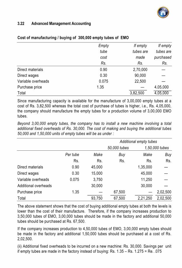
Advanced Management Accounting 3.22
Cost of manufacturing / buying of 300,000 empty tubes of EMO
Empty If empty If empty tube tubes are tubes are cost made purchased Rs. Rs. Rs. Direct materials 0.90 2,70,000 — Direct wages 0.30 90,000 — Variable overheads 0.075 22,500 — Purchase price 1.35 — 4,05,000 Total 3,82,500 4,05,000
Since manufacturing capacity is available for the manufacture of 3,00,000 empty tubes at a cost of Rs. 3,82,500 whereas the total cost of purchase of tubes is higher, i.e., Rs. 4,05,000, the company should manufacture the empty tubes for a production volume of 3,00,000 EMO tubes. Beyond 3,00,000 empty tubes, the company has to install a new machine involving a total additional fixed overheads of Rs. 30,000. The cost of making and buying the additional tubes 50,000 and 1,50,000 units of empty tubes will be as under :
Additional empty tubes 50,000 tubes 1,50,000 tubes Per tube Make Buy Make Buy Rs. Rs. Rs. Rs. Rs. Direct materials 0.90 45,000 1,35,000 — Direct wages 0.30 15,000 45,000 — Variable overheads 0.075 3,750 11,250 — Additional overheads 30,000 30,000 — Purchase price 1.35 — 67,500 — 2,02,500 Total 93,750 67,500 2,21,250 2,02,500
The above statement shows that the cost of buying additional empty tubes at both the levels is lower than the cost of their manufacture. Therefore, if the company increases production to 3,50,000 tubes of EMO, 3,00,000 tubes should be made in the factory and additional 50,000 tubes should be purchased at Rs. 67,500. If the company increases production to 4,50,000 tubes of EMO, 3,00,000 empty tubes should be made in the factory and additional 1,50,000 tubes should be purchased at a cost of Rs. 2,02,500. (ii) Additional fixed overheads to be incurred on a new machine: Rs. 30,000. Savings per unit if empty tubes are made in the factory instead of buying: Rs. 1.35 – Rs. 1.275 = Re. .075

CVP Analysis and Decision Making 3.23
Minimum additional quantity of empty tubes to be made to recover the additional fixed costs: RsRs
. ,. .30 0000 075 = 4,00,000 empty tubes
Thus the company should sell 3,00,000 + 4,00,000 = 7,00,000 tubes of EMO per month to warrant justification for the installation of the new machine for the manufacture of empty tubes. (iii) Evaluation of the profitability on sale of EMO at the three levels
Per tube 3,00,000 tubes 3,50,000 tubes 4,50,000 tubes Rs. Rs. Rs. Rs. Sales (Rs. 240/24 tubes) 10 30,00,000 35,00,000 45,00,000 Direct materials 3.60 10,80,000 12,60,000 16,20,000 Direct wages 2.70 8,10,000 9,45,000 12,15,000 Variable overheads 0.675 2,02,500 2,36,250 3,03,750 Empty tubes made 1.275 3,82,500 3,82,500 3,82,500 Empty tubes purchased 1.35 — 67,500 2,02,500 Total costs 24,75,000 28,91,250 37,23,750 Profit 5,25,000 6,08,750 7,76,250
Illustration : Make or Buy Decision A firm needs a component in an assembly operation. If it wants to do the manufacturing itself, it would need to buy a machine for Rs. 4 lakhs which would last for 4 years with no salvage value. Manufacturing costs in each of the 4 years would be Rs. 6 lakhs, Rs. 7 lakhs, Rs. 8 lakhs and 10 lakhs respectively. If the firm had to buy the component from a supplier the component would cost Rs. 9 lakhs, Rs. 10 lakhs, Rs. 11 lakhs and Rs. 14 lakhs respectively in each of the 4 years. However, the machine would occupy floor space which could have been used for another machine. This latter machine could be hired at no cost to manufacture an item, the sale of which would produce net cash flows in each of the 4 years of Rs. 2 lakhs; it is impossible to find room for both the machines and there are no other external effects. The cost of capital is 10% and PV factor for each of the 4 years is 0.909, 0.826, 0.751 and 0.683 respectively. Should the firm make the component or buy from outside? Solution
Evaluation of Make or Buy Proposal Rs. in lakhs
Year Present value When the Component When the Component factor at 10% is manufactured is bought
Cash outflow Present value Cash outflow Present value 0 1.000 4 4.000 — — 1 .909 6 + 2 7.272 9 8.181

Advanced Management Accounting 3.24
2 .826 7 + 2 7.434 10 8.260 3 .751 8 + 2 7.510 11 8.261 4 .683 10 + 2 8.196 14 9.562 34.412 34.264
Saving in buying: Rs. 34.412 lakhs – Rs. 34.264 lakhs = Rs. 0.148 lakh Thus it is beneficial to buy the component from outside. Note : The loss of Rs 2 lakhs cash inflow for each of the 4 years due to inability of the firm to operate another machine when it manufactures the component is to be treated as an opportunity cost. Illustration : Make or Buy decision Product ‘A’ takes five hours to produce on a particular machine and it has a selling price of Rs. 50 and a marginal cost of Rs. 35. On the same machine, another product ‘B’ can be made at two hours at a marginal cost of Rs. 5 per unit. Supplier’s price of product ‘B’ is Rs. 10 per unit. Assuming that machine hour is the key factor, advise whether product ‘B’ could be bought out or manufactured. Solution Rs. Selling price per unit of product ‘A’ 50 Less: Marginal cost per unit 35 Contribution per unit 15 Contribution per hour of product ‘A’ 3 (Rs. 15/5 hours) Since one unit of product ‘B’ needs 2 hours, therefore if a unit of B is produced, then the contribution lost by not producing ‘A’ = 2 hours × Rs. 3 = Rs. 6 Real cost of producing one unit of product ‘B’ Rs. Marginal cost per unit 5 Add: Contribution lost per unit 6 Total cost of producing a unit of Product ‘B’ 11 As the suppliers price per unit of product ‘B’ is Rs. 10 and that of producing in the factory is Rs. 11, therefore it is suggested that it is better to buy product ‘B’ from outside.

CVP Analysis and Decision Making 3.25
Illustration : Make or buy decision A machine manufactures 10,000 units of a part at a total cost of Rs. 21 of which Rs. 18 is variable. This part is readily available in the market at Rs. 19 per unit. If the part is purchased from the market then the machine can either be utilised to manufacture a component in same quantity contributing Rs. 2 per component or it can be hired out at Rs. 21,000. Recommend which of the alternative is profitable. Solution 1st alternative : (10,000 units of the part are manufactured internally). Variable cost of 10,000 units @ Rs. 18 p.u. (Rs.) 1,80,000 2nd alternative : (10,000 units of the part are purchased from the market and the machine is utilised to manufacture 10,000 units of a component contributing Rs.2/- per unit) Purchase cost of 10,000 units @ Rs.19/- p.u. (Rs.) 1,90,000 Less : Contribution received on the utilisation of machine time 10,000 units × Rs. 2 20,000 1,70,000 3rd alternative : (10,000 units of the part are purchased from outside and the machine time is hired out at Rs. 21,000). Purchase cost of 10,000 units @ Rs.19/- p.u. (Rs.) 1,90,000 Less : Rent received on hiring out the machine21,000 1,69,000

Advanced Management Accounting 3.26
Recommendation : Out of the above three alternatives, 3rd alternative is the best, as the cost of 10,000 required units under it is the lowest.
3.5 SHUT DOWN OR CONTINUE DECISION Very often it becomes necessary for a firm to temporarily close down the factory due to trade recession with a view to reopening it in the future. In such cases, the decision should be based on the marginal cost analysis. If the products are making a contribution towards fixed expenses or in other words if selling price is above the marginal cost, it is preferable to continue because the losses are minimised. By suspending the manufacture, certain fixed expenses can be avoided and certain extra fixed expenses may be incurred depending upon the nature of the industry, say, for example, extra cost incurred in protecting the machinery. So the decision is based on as to whether the contribution is more than the difference between the fixed expenses incurred in normal operation and the fixed expenses incurred when the plant is shut down. In other words, the shut down point is calculated by using the formula:
Shut down point = Total Shut
Contributifixed cost down
on per unit– costs
Illustration Rs. Fixed expenses at 50% activity 15,000 Fixed expenses when the factory is shut down 10,000 Additional expenses in closing down 1,000 Production at 50% activity = 5,000 units Contribution per unit Re. 1
Solution Rs. A. If the plant is shut down the sunk costs or fixed expenses 11,000 B. If it is working at 50% activity the fixed expenses 15,000 C. Additional fixed expenses : [(B) – (A)] 4,000 D. Contribution (5,000 units × Re. 1 p.u.) 5,000
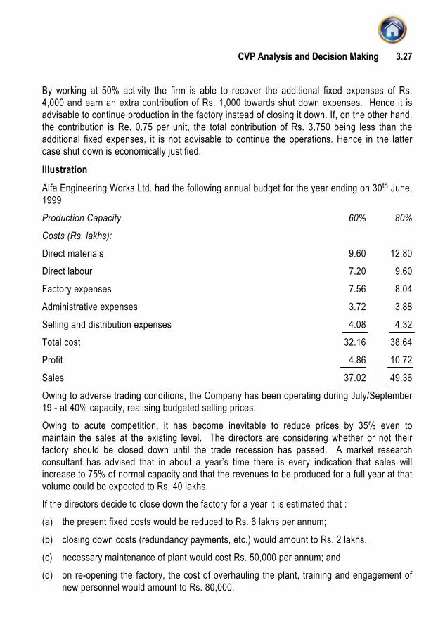
CVP Analysis and Decision Making 3.27
By working at 50% activity the firm is able to recover the additional fixed expenses of Rs. 4,000 and earn an extra contribution of Rs. 1,000 towards shut down expenses. Hence it is advisable to continue production in the factory instead of closing it down. If, on the other hand, the contribution is Re. 0.75 per unit, the total contribution of Rs. 3,750 being less than the additional fixed expenses, it is not advisable to continue the operations. Hence in the latter case shut down is economically justified.
Illustration
Alfa Engineering Works Ltd. had the following annual budget for the year ending on 30th June, 1999 Production Capacity 60% 80% Costs (Rs. lakhs): Direct materials 9.60 12.80 Direct labour 7.20 9.60 Factory expenses 7.56 8.04 Administrative expenses 3.72 3.88 Selling and distribution expenses 4.08 4.32 Total cost 32.16 38.64 Profit 4.86 10.72 Sales 37.02 49.36 Owing to adverse trading conditions, the Company has been operating during July/September 19 - at 40% capacity, realising budgeted selling prices. Owing to acute competition, it has become inevitable to reduce prices by 35% even to maintain the sales at the existing level. The directors are considering whether or not their factory should be closed down until the trade recession has passed. A market research consultant has advised that in about a year’s time there is every indication that sales will increase to 75% of normal capacity and that the revenues to be produced for a full year at that volume could be expected to Rs. 40 lakhs. If the directors decide to close down the factory for a year it is estimated that : (a) the present fixed costs would be reduced to Rs. 6 lakhs per annum; (b) closing down costs (redundancy payments, etc.) would amount to Rs. 2 lakhs. (c) necessary maintenance of plant would cost Rs. 50,000 per annum; and (d) on re-opening the factory, the cost of overhauling the plant, training and engagement of
new personnel would amount to Rs. 80,000.

Advanced Management Accounting 3.28
Prepare a report for the directors, making your recommendations. Solution The Directors, Alfa Engineering Works Ltd. New Delhi Dear Sir, As desired, we have analysed the cost implications of the decision of temporary closure of the trade recession. We find that if the factory is run at 40% capacity and with reduced selling prices, the loss likely to be incurred in one full year (the estimated period of recession), would be around Rs. 7.17 lakhs as detailed below: Rs.
(in lakhs) Direct materials 6.40 Direct labour 4.80 Factory expenses 7.08 Administrative expenses 3.56 Selling & distribution expenses 3.84 25.68 Loss 7.17
Sales
××
10075
6040lakhs02.37.Rs 18.51
If the factory is closed, the following costs will be incurred: Rs.
(in lakhs) Fixed costs 6.0 Closing down costs 2.0 Maintenance costs 0.5 Cost of overhauling the plant, training and engagement of staff 0.8 9.3

CVP Analysis and Decision Making 3.29
It is obvious from the above, that despite the fact that running at 40% capacity would imply a loss of Rs. 7.17 lakhs, it is better not to close down the factory since in that case the loss would be higher. In our views, even if running the factory entailed a somewhat bigger loss as compared to the loss incurred by closing it down temporarily, it may be better to keep the factory in operation. This is because a closure, even if temporary, results in the loss of regular and old customers, suppliers and skilled personnel. This, coupled with a loss of goodwill in the market, may give rise to substantial losses at the time of restarting the factory. We trust that the above analysis would be helpful to you in reaching an appropriate decision in the matter. We shall be glad to be of any further assistance that may be required in this regard.
Yours faithfully, X & Co.
Chartered Accountants. Working note:
Factory Admn. Selling expenses expenses expenses (Rs. lakhs) (Rs. lakhs) (Rs. lakhs)
(i) Amount at 60% 7.56 3.72 4.08 (ii) Amount at 80% 8.04 3.88 4.32 (iii) Change for 20% 0.48 0.16 0.24 (iv) Amount at 40% (i) – (iii) 7.08 3.56 3.84
Illustration A paint manufacturing company manufactures 2,00,000 per annum medium-sized tins of “Spray Lac Paints” when working at normal capacity. It incurs the following costs of manufacturing per unit : Rs. Direct material 7.80 Direct labour 2.10 Variable overhead 2.50 Fixed overhead 4.00 Product cost (per unit) 16.40

Advanced Management Accounting 3.30
Each unit (tin) of the product is sold for Rs. 21 with variable selling and administrative expenses of 60 paise per tin. During the next quarter only 10,000 units can be produced and sold. Management plans to shut down the plant estimating that the fixed manufacturing cost can be reduced to Rs. 74,000 for the quarter. When the plant is operating, the fixed overheads are incurred at a uniform rate throughout the year. Additional costs of plant shut-down for the quarter are estimated at Rs. 14,000. You are required: (a) To express your opinion, along with the calculations, as to whether the plant should be
shut down during the quarter, and (b) To calculate the shut down point for quarter in units of products (i.e., in terms of number
of tins).
Solution (a) Working note: Contribution per tin:
Selling price – Variable cost of the product = Rs. 21 – Rs. (7.80 + 2.10 + 2.50 + 0.60) = Rs. 8 per tin Calculation of loss, if plant is operated Rs. Total contribution on 10,000 tins @ Rs. 8 each 80,000 Less: Total fixed cost for three months
(2,00,000 × Rs. 4) × 312
2,00,000
Expected loss on operation (1,20,000)
Calculation of loss (shut down costs) if plant is shut down Rs. Unavoidable fixed cost 74,000 Additional cost of shut-down 14,000 Total loss on shut down (88,000) It is clear from the above, that if plant is operated, loss would be Rs. 1,20,000 which exceeds the loss by Rs. 32,000 (Rs. 1,20,000 – Rs. 88,000) when the plant is shut-down. Therefore, the management should shut-down the plant during the quarter.

CVP Analysis and Decision Making 3.31
(b) Calculation of shut-down point Avoidable fixed cost for the period (or fixed cost which will not be incurred if the plant is shut down) : = Total fixed cost for the period – (Unavoidable fixed costs + Additional shut down costs) = Rs. 2,00,000 – (Rs. 74,000 + Rs. 14,000) = Rs. 2,00,000 – Rs. 88,000 = Rs. 1,12,000
Shut-down point = Avoidable fixed costContribution per unit
= Rs.Rs1,12,000
. 8 = 14,000 tins
or
Shut-down point = Total fixed cost – Shut down costs
Contribution per unit
= Rs. 2,00,000 – Rs.88,000
Rs.8 = 14,000 tins
Other considerations in shut down decisions : Cost is not the only criterion for deciding in favour of shut down. Non-cost factors worthy of consideration in this regard are : 1. Interest of the workers —if the workers are discharged it may become difficult to get
skilled workers later, on reopening of the factory. Also shut down may create problem for the workers which may far exceed the cost benefits of the shut down.
2. Once the firm is closed down competitors may establish their products and thus it may be difficult to introduce the product in the market again.
3. The plant may become obsolete or depreciate at a larger rate when not in operation. Thus, heavy capital expenditure may have to be incurred on re-opening.
Illustration Universe Ltd. manufactures 20,000 units of ‘X’ in a year at its normal production capacity. The unit cost as to variable costs and fixed costs at this level are Rs.13 and Rs.4 respectively. Due to trade depression, it is expected that only 2,000 units of ‘X’ can be sold during the next year. The management plans to shut-down the plant. The fixed costs for the next year then is expected to be reduced to Rs. 33,000. Additional costs of plant shut-down are expected at Rs. 12,000. Should the plant be shut-down ? What is the shut-down point ?

Advanced Management Accounting 3.32
Solution Note : The decisions regarding the plant to shut-down and the calculation of shut-down point requires the figure of selling price per unit of the units sold. As the statement of the question fails to indicate the selling price (per unit) therefore one is free to assume it. Assumption : Let’s assume the Selling Price per unit be Rs. 20 Statement of cost for taking a decision about shut-down of plant
Plant is operated Plant is shut down Rs. Rs. Variable Cost 26,000 – (2,000 units × Rs. 13) Fixed Costs 80,000 33,000 (20,000 units × Rs. 4) (unescapable cost) Additional shut down cost – 12,000 Total Cost 1,06,000 45,000 State of loss : Sales 40,000 – (2,000 units × Rs. 20) Less : Total Cost 1,06,000 45,000 (as above) Loss (66,000) (45,000) (if continued) (if shut-down) Recommendation : A comparison of loss figures indicated as above points out, that, loss
is reduced if the plant is shut-down. In fact by doing so the concern’s loss would be reduced by (Rs. 21,000).
Calculation of Shut down point :
Shut–down point = Total fixed cost Shut down costsContribution per unit
−
= Rs.80,000 Rs. 45,000Rs. 20 Rs.13
−−
= 5,000 units 3.6 EXPORT V/s LOCAL SALE DECISION When the firm is catering to the needs of the local market and surplus capacity is still available, it may think of utilising the same to meet export orders at price lower than that prevailing in the local market.

CVP Analysis and Decision Making 3.33
This decision is made only when the local sale is earning a profit, i.e., where its fixed expenses have already been recovered by the local sales. In such cases, if the export price is more than the marginal cost, it is preferable to enter the export market. Any reduction in the price prevailing in the local market to fulfil surplus capacity may have adverse effect on the normal local sales. Dumping in the export market at a lower price will not, however, have any such adverse effect on local sales. Illustration A firm gives the following data : Selling price Rs. 6 per unit Fixed expenses Rs. 15,000 Total cost Rs. 5 per unit Marginal cost Rs. 4 per unit Local sales 15,000 units Capacity of the plant 20,000 units Export order received for 3,000 units at Rs. 4.50 per unit. Advise whether to accept the export order or not. Solution
Break-even point = Fixed expensesContribution
= 4.Rs–6.Rs
000,15.Rs = 2.Rs000,15.Rs
= 7,500 units Since fixed expenses are recovered at this level of output, any price above the marginal cost will fetch additional profit. So the export selling price of Rs. 4.50 will fetch an additional profits of Rs. 1,500 as under : 3,000 units × (Rs. 4.50 – Rs. 4.00) = Rs. 1,500 Since the goods are sold in the export market, it will not have any adverse effect on the local selling price of Rs. 6 per unit. Illustration X Ltd., having an installed capacity of 1,00,000 units of a product is currently operating at 70% utilization. At current levels of input prices, the FOB unit costs (after taking credit for applicable export incentives) work out as follows: Capacity Utilisation FOB Unit Costs Per cent Rs. 70 97 80 92 90 87 100 82

Advanced Management Accounting 3.34
The company has received three foreign offers from different sources as under: Source A 5,000 units at Rs. 55 per unit FOB Source B 10,000 units at Rs. 52 per unit FOB Source C 10,000 units at Rs. 51 per unit FOB Advise the company as to whether any or all export orders should be accepted or not.
Solution X Limited
Statement showing Differential Cost at Different Capacity Utilisation Levels Installed capacity 1,00,000 Units
Capacity Production at FOB unit Total Differential Per unit utilisation different levels costs costs costs differential of capacity costs utilisation Percent Units Rs. Rs. Rs. Rs. 70 70,000 97 67,90,000 — — 80 80,000 92 73,60,000 5,70,000 57 90 90,000 87 78,30,000 4,70,000 47 100 1,00,000 82 82,00,000 3,70,000 37
Statement showing Gain or Loss on Accepting the Various Export Orders
Export Export Capacity Differential Costs FOB Sales Gain/ Order Order Utilisation Price Revenue (Loss) (Source) (Unit) Per cent Per Total per from the Unit Unit Export Rs. Rs. Rs. Rs. Rs. A 5,000 75% 5,000 Uts. 2,85,000 55 2,75,000 (10,000) @ 57 B 10,000 85% 5,000 Uts. @ 57 5,20,000 52 5,20,000 Nil 5,000 Uts. @ 47 C 10,000 95% 5,000 Uts. @ 47 4,20,000 51 5,10,000 90,000 5,000 Uts. @ 37
Total 25,000 95% 12,25,000 13,05,000 80,000

CVP Analysis and Decision Making 3.35
It is obvious from the above statement that the company will gain only when all the three export orders are accepted. If the company accepts exports only for one or two of the three sources, it will loose. Therefore, the company should accept all the three exports orders. 3.7 EXPAND OR CONTRACT DECISION Whenever a decision is to be taken as to whether the capacity is to be expanded or not, consideration should be given to the following points: (a) Additional fixed expenses to be incurred. (b) Possible decrease in selling price due to increase in production. (c) Whether the demand is sufficient to absorb the increased production. Based on these considerations, the cost schedule will be worked out. While deciding about the contraction of business, the saving in fixed expenses and the marginal contribution lost will have to be taken into account. If a branch office is to be closed down, and if the branch is giving a marginal contribution sufficient to cover fixed expenses the contraction may lead to a loss as under : Example Branch B : Sales Rs. 20,000 P/V ratio 20% Marginal contribution Rs. 4,000 Fixed expenses of the branch Rs. 3,000 The branch is giving an extra contribution of Rs. 1,000. If it is closed, the fixed expenses saving is Rs. 3,000 whereas the contribution lost is Rs. 4,000. Hence it is not advisable to contract the business by closing down the branch. Illustration Nice and Warm Ltd., manufactures and markets hot plates. During the first five years of operation, the company had experienced a gradual increase in sales volume, and the current annual growth in sales of 5% is expected to continue into the foreseeable future. The plant is now producing at its full capacity of one lakh hot plates. At the monthly Management Advisory Committee meeting, amongst other things, the plan of action for next year was discussed. Managing Director proposed two alternatives. First, operations could be continued at full capacity and with the existing facilities an output of one lakh hot plates at a selling price of Rs. 100 per unit could be maintained. Secondly, production and sales could be increased by 5% to take advantage of the rate of expansion in demand for the product. But this could increase cost, as to achieve the output, the company will have to resort to weekend and overtime workings. However, a policy of steady growth was preferable to maintaining status quo.

Advanced Management Accounting 3.36
In view of the company’s competitors having a substantial share of the market, the Works Director was of the view that it was not enough for the company to maintain merely the present share of the total market. A larger share of the total market should be obtained. For that, the company should increase the production by 10% through a modest expansion of plant capacity. In order to sell the output of 1,10,000 units, the selling price could be reduced to Rs. 95 per unit. Thinking on the same lines, the Marketing Director put forth a more radical proposal. The strategy should be to seize the competitive leadership in the market with regard to both price and volume. With this end in view, he suggested that the company should straight away embark on an expensive modernisation programme which will initially increase volume by 20%. The entire output of 1,20,000 hot plates could be easily sold at a price of Rs. 90 per unit. At this juncture Managing Director expressed concern about the probable behaviour of the company’s competitors. They might also expand in order to produce more and sell at lowest prices. Suppose this happened, he wanted also the financial effects of the proposals of the Works Director and the Marketing Director, if in those proposals, the increase in sales were to be only half of that predicted. As the Cost Accountant of the company you are required to critically evaluate the six alternatives, along with your recommendations and circulate the same to the Directors. In this connection you have gathered the following details., (1) If next year’s production was maintained at the current year’s level variable costs would
remain unchanged at Rs. 30 lakhs. (2) The weekend and overtime working would increase with the variable and fixed costs.
Variable cost would rise to Rs. 55 per unit while fixed costs would increase to Rs.30,25,000.
(3) In the proposal of the Works Director, the ratio of variable costs to sales would continue to be 50% and fixed costs would rise to Rs. 32,25,000.
(4) In the proposal of the Marketing Director, as a result of increased production efficiency and some savings from purchase of materials, it is estimated that the ratio of variable cost to sales would decrease to 48% and the fixed costs would increase by Rs. 5,16,000.
Your answer should contain: (a) A tabular statement of comparative figures pertaining to Total Turnover, Total
Contribution, Percentage of Profit to Sales and Break-Even units as regards to each of the six proposals.
(b) Comment on the relative risks involved. (c) Consideration of the short-term and long-term implications of the Managing Director’s
proposals.

CVP Analysis and Decision Making 3.37
(d) Comments on the price elasticity of demand for the company’s product and your suggestions on the pricing policy and cost structure.
(e) Comments on financial implications of the expansion schemes. (a) Tabular Statement of Comparative Figures Pertaining to Total Turnover, Total
Contribution, Percentage of Profit to Sales and Break-even Units etc., as regards to each of the Six Proposals.
Proposals
Managing Managing Works Works Marketing Marketing
Director’s Director’s Director’s Director’s Director’s Director’s
1st Proposal 2nd Proposal 1st Proposal 2nd Proposal 1st 2nd Proposal
(1/2 of ex- Proposal (1/2 of
pected expected
increase) increase)
(1) (2) (3) (4) (5) (6)
Units sold 1,00,000 1,05,000 1,10,000 1,05,000 1,20,000 1,10,000
Unit selling
price (Rs.) 100 100 95 95 90 90
Total turnover
(Rs. in lakhs) 100.00 105.00 104.50 99.75 108.00 99.00
Unit contribution (Rs.) 50 45 47.5 47.5 46.80 46.80
Total contribution
(Rs. in lakhs) 50 47.25 52.25 49.875 56.16 51.48
Fixed cost (Rs. in lakhs) 30 30.25 32.25 32.25 35.16 35.16
Profit (Rs. in lakhs) 20 17.00 20.00 17.625 21 16.32
Percentage of
profit to sales 20% 16.19% 19.14% 17.67% 19.44% 16.48%
Break-even units 60,000 67,222 67,895 67,895 75,128 75,128
Margin of safety
in units 40,000 37,778 42,105 37,105 44,872 34,872

Advanced Management Accounting 3.38
Solution (a) For this part refer to page 3.34. (b) At the present full capacity level, it is enough to sell 60,000 units to break even. Other
proposals raise the break-even point further. In an uncertain market, if in the proposals of Works Director and the Marketing Director, only half the increase is achieved, the margin of safety will be lower than the present 40,000 units. Profit as a percentage of sales is also lower than existing, in all the proposals. All this is a disquieting feature as the risk involved is greater in all the other proposals.
(c) The company has already reached its full capacity. As a short term measure, the Managing Director’s first proposal seems to be all right. From long-term point of view, neither of the proposals can be considered to be satisfactory. Both the proposals of the Managing Director do not provide a lasting solution. Though the second proposal maintains the market share, it results in less profit, both in quantum and percentage. As the capacity has already been reached there is an urgent necessity for the Managing Director to address himself to long range objectives and plans keeping in view the expansion in demand for the company’s product.
(d) It seems that both the Works Director and the Marketing Director have very elementary notions on price. They think that if the volume increases in order to sell the increased volume, price has to be lowered. No serious study seems to have been made on the price elasticity of demand for the company’s product. On the other hand, we have been told that there is a steady 5% annual growth in demand, which means that the prices need not be reduced, only more market share has to be obtained. For incremental production, differential pricing in certain special markets has to be resorted to; if this is not possible, the increased production can be sold under a different brand name with a different price (A static cost structure, more or less, has been assumed). To beat competition, a better product has to be put in the market and cost reduction offered through value analysis, etc.
(e) The expansion scheme envisaged have to be properly tested for profitability by feasibility study reports, etc. Source of financing the expansion has to be determined. The financial implications of share issue or borrowed funds have to be gone through. Long range objectives have to be defined and plans drawn accordingly to achieve them.
3.8 PRODUCT MIX DECISION Many times the management has to take a decision whether to produce one product or another instead. Generally decision is made on the basis of contribution of each product. Other things being the same the product which yields the highest contribution is best one to produce. But, if there is shortage or limited supply of certain other resources which may act as a key factor like for example, the machine hours, then the contribution is linked with such a key factor for taking a decision. For example, in an undertaking the availability of machine capacity is limited and the machine hours required for one unit of the two products are

CVP Analysis and Decision Making 3.39
different. In such cases the contribution is to be linked with the machine hour and the product which yields the highest contribution per machine hour is to be preferred for taking decision.
Illustration There are two products A and B. The selling prices, variable costs and machine hours required per unit are: A B Selling price (Rs.) 2.00 2.50 Variable cost (Rs.) 1.00 1.50 Machine hours 2 1 Find the more profitable product when plant capacity is limited.
Solution Selling price (Rs.) 2.00 2.50 Less : Variable cost (Rs.) 1.00 1.50 Contribution (Rs.) 1.00 1.00 Machine hours required 2 1 Contribution per machine hours (Rs.) 0.50 1.00 From the above it is evident that the contribution of product A & B in absolute terms is the same. However, when we link this contribution with the machine hour which is a key factor, the product ‘B’ gives more profit. As such, product ‘B’ is to be given preference over product ‘A’.
Illustration A firm manufactures 5 products using the same raw materials which is in short supply. By examining the following information, show which product is to be chosen so that the profit can be the maximum.
Products A B C D E Sales (units) 1,500 2,500 1,600 2,000 2,200 Production (units) 2,000 3,000 1,500 2,000 2,000 Possible sales 1,500 2,500 1,500 2,000 2,000 Selling price per unit 4.00 3.50 1.50 1.00 3.00 Marginal cost per unit 3.00 2.00 1.25 0.75 2.50 Contribution per unit 1.00 1.50 0.25 0.25 0.50 Raw material required (kgs.) 2 8 3 5 2 Contribution against 1 kg. of raw material 0.50 0.19 0.083 0.05 0.25

Advanced Management Accounting 3.40
Solution When raw material is in short supply, the order in which production is to be undertaken is A, E, B, C, D based on contribution per unit of the key factor. Let us suppose that 5,000 kgs. of raw material is available. Our production pattern will be as under:
Product Sales Material Total Contribution Total units per unit material per unit contribution kgs. kgs. Rs. Rs.
A 1,500 2 3,000 1.00 1,500 E 1,000 2 2,000 0.50 500
5,000 2,000
Although the unit contribution of product B is the largest, when the key factor is raw material supply, it ranks third in priority for manufacture, because it consumes more raw material. Illustration (a) Alcos Ltd., manufactures and sells four types of products under the brand names A, B, C
and D. The sales mix in value comprises 33-1/3%, 41-2/3%, 16-2/3% and 8-1/3% of A, B, C and D respectively. The total budgeted sales (10%) are Rs. 60,000 per month.
Operating costs are : Variable costs: A 60% of selling price B 68% of selling price C 80% of selling price D 40% of selling price Fixed costs – Rs. 14,700 per month. Calculate the break-even point for the products on an overall basis. (b) It has been proposed to change the sales mix as follows, the total sales per month
remaining Rs. 60,000. A 25% B 40% C 30% D 5%

CVP Analysis and Decision Making 3.41
Assuming that the proposal is implemented. Calculate the new break-even point. Solution (a)
Products
A B C D Total
Sales mix 33% 41% l6% 8% 100% Rs. Rs. Rs. Rs. Rs. Sales 20,000 25,000 10,000 5,000 60,000 Variable cost 12,000 17,000 8,000 2,000 39,000 Contribution 8,000 8,000 2,000 3,000 21,000
P/V ratio:
ContributionSales
× 100 = Rs. 21,000Rs. 60,000
× 100 = 35%
Break-even point (Sales value): Fixed costsP / V ratio =
35.0700,14.Rs = Rs. 42,000
(b) The revised contribution after change in sales mix Products
A B C D Total Sales mix 25% 40% 30% 5% 100% Rs. Rs. Rs. Rs. Rs. Sales 15,000 24,000 18,000 3,000 60,000 Variable costs 9,000 16,320 14,400 1,200 40,920
Contribution 19,080
P/V ratio = RsRs
. ,
. ,19 08060 000 × 100 = 31.8%
Break-even point (Sales value) = Rs. ,.14 700
0 318 = Rs. 46,226.
Illustration A firm’s operations are at present performed by hand. It has a proposal to install a new machine which can produce at a faster rate. Following information is available. Advise the management about the profitability of mechanisation.

Advanced Management Accounting 3.42
Hand Machine Production in units per hour 1 2 Marginal cost per unit (Rs.) 18 16 Additional fixed cost per unit (Rs.) — 3 Total cost per unit (Rs.) 18 19 Selling price per unit (Rs.) 24 24
Solution Let us analyse the figures as under: Hand Machine Rs. Rs. Selling price per unit 24 24 Less: Marginal cost per unit 18 19 (including additional fixed cost) Contribution per unit 6 5 Contribution per hour 6 10 If there is a great demand for the products, it is advisable to mechanise because the gross margin per hour is more than that under hand operation. If however, there is idle capacity and there is an under- absorption of fixed overheads to the extent of Rs. 3 per unit the total cost will be Rs. (19 + 3) = Rs. 22 leaving a contribution of Rs. 2 per unit. The contribution per hour will, therefore, be Rs. 4 which is less than that of obtaining under hand operation. Hence mechanisation will not be advisable under these circumstances. Illustration An engineering company is engaged in producing four products through operations at welding and pressing departments. Products W1 and W2 are produced by welders in the welding department whereas products P1 and P2 are produced by press-operators in the pressing department. Due to specific skill requirements, the welders and press-operators can only work in their own department. The following relevant data are available in respect of the products: Products W1 W2 P1 P2
Hours required per unit 4 4 5 2 Selling price per unit (Rs.) 48 50 77 69

CVP Analysis and Decision Making 3.43
Direct material cost per unit (Rs.) 18 22 32 44 Direct labour hourly rate (Rs.) 4 4 4 4 Variable overhead rate per unit (Rs.) 2 2 3 3 The company incurs Rs. 50,000 per annum towards fixed costs. The maximum available hours are 20,000 and 16,000 for welding and pressing departments respectively. The demands keep on fluctuating but the minimum demands which are to be met as per management’s decision are 2,000 units of Wl, 2,500 units of W2, 1,800 units of P1 and 2,200 units of P2.
The production manager suggests that the welders and press- operators can be trained to perform both welding and pressing jobs so that excess demand of any of the products can be met. This decision is going to increase the burden of fixed costs by Rs. 5,000 per annum. Prepare the profitability statement for optimum product-mix and recommend with reasons and appropriate workings whether it is advisable to train the welders and press-operators as suggested by the production manager.
Solution Optimum Product Mix Before Training
Department Welding Pressing Maximum Hours 20,000 hours 16,000 hours Product W1 W2 P1 P2
Selling price per unit (Rs.) 48 50 77 69 Less: Variable cost
Material (Rs.) 18 22 32 44 Labour (Rs.) 16 16 20 8 Variable overhead (Rs.) 2 2 3 3
Total variable cost (Rs.) 36 40 55 55 Contribution per unit : (A) 12 10 22 14 Labour hours per unit : (B) 4 4 5 2 Contribution per hour (Rs.) (A) (B) 3 2.5 4.4 7 Ranking I II II I Minimum production (units) 2,000 2,500 1,800 2,200 Labour hours needed 8,000 10,000 9,000 4,400 Labour hours used for each department 8,000 + 10,000 = 18,000 9,000 + 4,400= 13,400

Advanced Management Accounting 3.44
Balance hours available 20,000 – 18,000 = 2,000 16,000 – 13,400 = 2,600 Product to be produced WI P2
Units to be produced 2,000/4 = 500 2,600/2 = 1,300 W1 W2 P1 P2
Hence, product-mix 2,000 + 500 2,500 1,800 2,200 +1,300 (units) = 2,500 = 3,500 Profitability Statement before Training
Product Product-mix Hours Contribution units Per unit Total Per hour Total Rs. Rs. W1 2,500 4 10,000 3.00 30,000
W2 2,500 4 10,000 2.50 25,000
20,000 55,000 P1 1,800 5 9,000 4.40 39,600
P2 3,500 2 7,000 7.00 49,000
16,000 88,600 Total 36,000 1,43,600 Less: Fixed costs 50,000 Net profit 93,600 Optimum Product-Mix After Training After training, the capacity will be taken as a whole at 36,000 labour hours because of interchangeability of available labour force. The ranking will be done on the basis of contribution per hour among all the four products, since a workman is trained to work in any of the departments. Production W1 W2 P1 P2
Maximum hours 36,000 hours as a whole Hours needed for minimum production 8,000 10,000 9,000 4,400 (Total hours = 31,400 hours) Balance hours (36,000 – 31,400 hours = 4,600 hours) Product priority (Ranking) III IV II I Product in balance hours P2 (I rank): 4,600 ÷ 2 = 2,300 units
Product-mix (units) 2,000 2,500 1,800 2,200 + 2,300 = 4,500

CVP Analysis and Decision Making 3.45
Profitability Statement After Training
Product Product-mix Hours Contribution
units Per unit Total Per hour Amount
Rs. Rs. Rs.
W1 2,000 4 8,000 3.00 24,000
W2 2,500 4 10,000 2.50 25,000
P1 1,800 5 9,000 4.40 39,600
P2 4,500 2 9,000 7.00 63,000
36,000 1,51,600 Less: Fixed costs 55,000 Net profit 96,600 Recommendation: Since the net profit after training will be more by Rs. 3,000 (Rs. 96,600 – Rs. 93,600), it is advisable to train the welders and press operators as suggested by the production manager. Illustration Veejay Ltd. makes and sell two products, Vee and Jay. The budgeted selling price of Vee is Rs. 1,800 and that of Jay is Rs. 2,160. Variable costs associated with producing and selling the Vee are Rs. 900 and with Jay Rs. 1,800. Annual fixed production and selling costs of Veejay Ltd. are Rs. 88,000. The company has two production/sales option. The Vee and Jay can be sold either in the ratio of two Vees to three Jays or in the ratio of one Vee to two Jays. What will be the optimal mix and why ? Solution Selection of best optimal mix Products
Vee Jay Rs. Rs. Budgeted selling price p.u. 1,800 2,160 Less : Variable cost p.u. 900 1,800 Contribution p.u. 900 360

Advanced Management Accounting 3.46
(I) Production/Sales option : (2 units of Vee and 3 units of Jays)
Total contribution under 1st option = (2 units × Rs. 900 + 3 units × Rs. 360) = Rs. 1,800 + Rs. 1,080 = Rs. 2,880
Break-even point = Annual fixed production & selling costsTotal contribution under Ist option
= Rs.88,000Rs. 2,880 = 30.56 (sets of 5 units each)
Products
Vee Jay Total
Break-even point (units) 30.56 × 2 units 30.56 × 3 units = 61.12 units = 91.68 units = 61 (units approx.) = 92 (units approx.) Break–even sales (Rs) = 1,09,800 = 1,98,720 3,08520 (61 units × Rs. 1,800) (92 units × Rs. 2,160) (II) Production/Sales option : (1 unit of Vee and 2 units of Jays)
Total contribution under IInd option = (1 unit × Rs. 900 + 2 units × Rs. 360) = Rs. 900 + Rs. 720 = Rs. 1,620
Break–even point = Annual fixed production & selling costsTotal contribution under Ist option
= Rs.88,000Rs. 2,880
= 54.32 (sets of 3 units each)
Products
Vee Jay Total Break–even points (units) 54.32 × 1 unit54.32 × 2 units = 54 (units approx.) = 109 (units approx.) Break–even sales (Rs.) = 97,200 = 2,35,440 3,32,640 (54 units × Rs. 1,800) (109 units × Rs. 2,160) Note: The given amount of annual fixed production and selling cost is such that it fails to determine the exact figure of break–even point under two given sales options. The approximations made

CVP Analysis and Decision Making 3.47
in the above solutions under option I, at break–even lelvel over recovers Rs. 20; whereas under option II of the solution there is an under recovery of fixed cost to the extent of Rs. 160. Decision & reasoning : Option I is preferred over option II, as it results in a lower level of sales to reach break–even (because of higher average contribution per unit sold). The average contribution per unit (under option I) is Rs. 576 (Rs. 2,880/5 units) and (under option II) it is Rs. 540 (Rs. 1,620/3 units). Option I contains a higher percentage (40% as against 33 1/3%) of more profitable products. Illustration ZED Ltd. manufactures two products P and Q and sells them at Rs. 215 and Rs. 320 per unit respectively. The variable costs per unit are as under.
Product-P Product-Q
Rs. Rs.
Raw materials : Material-X 22.00 28.00 Material-Y 8.00 32.00 Direct wages (Rs.6 per labour hour) : Department-A 36.00 54.00 Department-B 18.00 36.00 Department-C 54.00 — Department-D — 72.00 Variable overheads 23.00 14.30
The company procures raw materials against import licence. The company operates at single shift a day of 8 hours for 300 days in a year. The number of workmen engaged are 30, 16, 18 and 24 in departments A, B, C and D respectively. Neither the workers are subject to transfer from one department to another nor any new recruitment is possible at present. Fixed costs are Rs. 12,000 per month. You are required to find out the following : (a) The product-mix to yield maximum profit (b) The most profitable product if only one product is to be manufactured. Whether the
answer will differ if licence to import raw materials is released only for Rs. 1,80,000.

Advanced Management Accounting 3.48
Solution Working Notes : 1. Computation of total labour hours available
Departments No. of workmen Days Hrs./day Total hours
(a) (b) (c) (d) (e) = (b) × (c) × (d)
A 30 300 8 72,000 B 16 300 8 38,400 C 18 300 8 43,200 D 24 300 8 57,600
2. Computation of hours required per unit of each product
Departments Product P Product Q
Wages Wages/hr. Hrs. Wages Wage/hr. Hrs
(Rs.) (Rs.) (Rs.) (Rs.)
(a) (b) (c) = (a)/(b) (d) (e) (f) = (d)/(e)
A 36 6 6 54 6 9 B 18 6 3 36 6 6 C 54 6 9 – – – D – – – 72 6 12 Total hours per unit : 18 27 3. Statement showing maximum output permissble
Departments Hours Product P Product Q
available Hrs. required/ Maximum Hrs. required/ Maximum
Unit output in Unit output in
Units Units
(a) (b) (c) = (a)/(b) (d) (e) = (a)/(d)
A 72,000 6 12,000 9 8,000 B 38,400 3 12,800 6 6,400 C 43,200 9 4,800* – – D 57,600 – 12 4,800* Total hours p.u. : 18 27
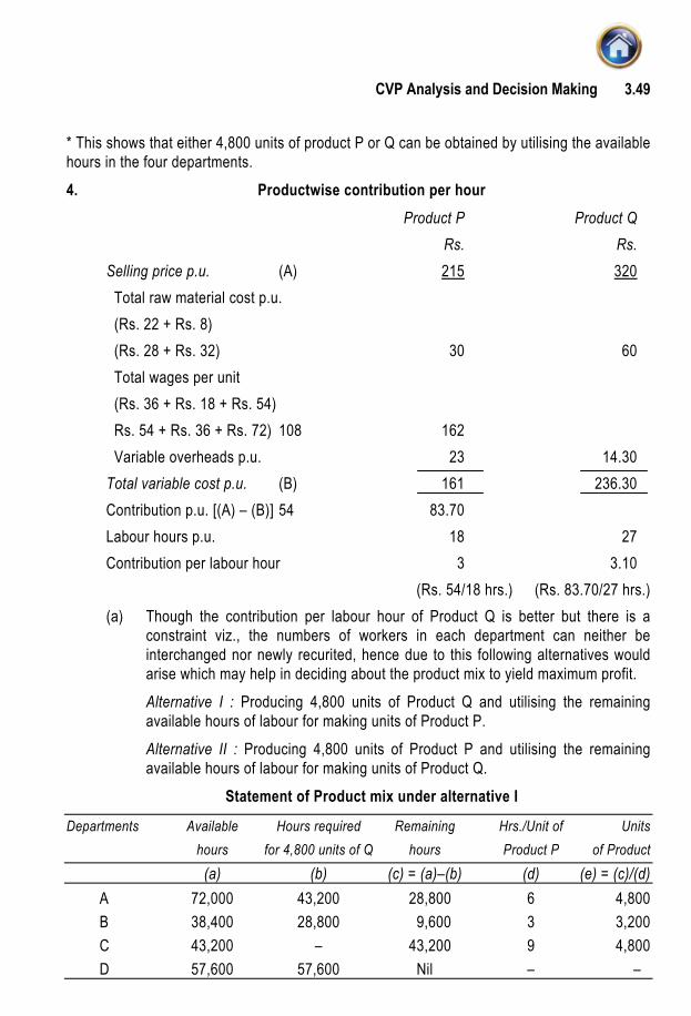
CVP Analysis and Decision Making 3.49
* This shows that either 4,800 units of product P or Q can be obtained by utilising the available hours in the four departments. 4. Productwise contribution per hour Product P Product Q Rs. Rs. Selling price p.u. (A) 215 320 Total raw material cost p.u. (Rs. 22 + Rs. 8) (Rs. 28 + Rs. 32) 30 60 Total wages per unit (Rs. 36 + Rs. 18 + Rs. 54) Rs. 54 + Rs. 36 + Rs. 72) 108 162 Variable overheads p.u. 23 14.30 Total variable cost p.u. (B) 161 236.30 Contribution p.u. [(A) – (B)] 54 83.70 Labour hours p.u. 18 27 Contribution per labour hour 3 3.10 (Rs. 54/18 hrs.) (Rs. 83.70/27 hrs.) (a) Though the contribution per labour hour of Product Q is better but there is a
constraint viz., the numbers of workers in each department can neither be interchanged nor newly recurited, hence due to this following alternatives would arise which may help in deciding about the product mix to yield maximum profit.
Alternative I : Producing 4,800 units of Product Q and utilising the remaining available hours of labour for making units of Product P.
Alternative II : Producing 4,800 units of Product P and utilising the remaining available hours of labour for making units of Product Q.
Statement of Product mix under alternative I
Departments Available Hours required Remaining Hrs./Unit of Units hours for 4,800 units of Q hours Product P of Product (a) (b) (c) = (a)–(b) (d) (e) = (c)/(d) A 72,000 43,200 28,800 6 4,800 B 38,400 28,800 9,600 3 3,200 C 43,200 – 43,200 9 4,800 D 57,600 57,600 Nil – –

Advanced Management Accounting 3.50
The above table shows that out of the available hours under alternative I; 4,800 units of Product Q and 3,200 units of Product P can be made. Statement of Product mix under alternative II
Departments Available Hours required Remaining Hrs./Unit of Units
hours for 4,800 units of P hours Product Q of Product
(a) (b) (c) = (a)–(b) (d) (e) = (c)/(d)
A 72,000 28,800 43,200 9 4,800 B 38,400 14,400 24,000 6 4,000 C 43,200 43,200 – – – D 57,600 – 57,600 12 4,800
The above table shows that out of the available hours under alternative II; 4,800 units of Product P and 4,000 units of Product Q can be made. Profit Statement under above alternatives
Products First alternative Second alternative
Units Contribution Amount Units Contribution Amount
p.u. (Rs.) Rs. p.u. (Rs.) Rs.
P 3,200 54.00 1,72,800 4,800 54.00 2,59,200 Q 4,800 83.70 4,01,760 4,000 83.70 3,34,800 Total Contribution: 5,74,560 5,94,000 Less : Fixed cost p.a. 1,44,000 1,44,000
Profit 4,30,560 4,50,000
Second alternative is the most profitable product mix. (b) Statement of most profitable product if only one product is to be manufactured
Products P Q
Contribution per unit (Rs.) : A 54.00 83.70 Maximum possible output (in units) : (B) 4,800 4,800 Total Contribution : (A) × (B) 2,59,200 4,01,760
Product Q is to be preferred

CVP Analysis and Decision Making 3.51
Statement of most profitable product if only one product is to be manufactured and licence to import the raw material is only
for materials worth Rs. 1,80,000 Products P Q
Raw material required p.u. (Rs.) 30 60 Permissible output in units out of imported material of Rs. 1,80,000 6,000 3,000 Maximum output possible in the available hours 4,800 4,800 Output possible keeping in view the the availability of imported material and labour hours (Units) 4,800 3,000 Contribution per unit (Rs.) 54 83.70 Total Contribution (Rs.) 2,59,200 2,51,100 (4,800 units × Rs. 54) (3,000 units × Rs. 83.70)
Product P is to be preferred (i.e. answer differs) because of import licence restriction, which is only available for purchasing material worth only Rs. 1,80,000 Illustration The relevant data of X Ltd. for its three products A, B and C are as under :
A B C
Direct material (Rs./Unit) 260 300 250 Direct labour (Rs./Unit) 130 270 260 Variable overheads (Rs./Unit) 110 230 180 Selling price (Rs./Unit) 860 1,040 930 Machine Hours required (Per Unit) 12 6 3
The estimated fixed overheads at four different levels of 3,600; 6,000; 8,400; and 10,800 machine hours are Rs. 1,00,000; Rs. 1,50,000; Rs. 2,20,000 and Rs. 3,00,000 respectively. The maximum demand of A, B and C in a cost period are 500; 300 and 1,800 units respectively. You are required to find out (i) the most profitable product-mix at each level and (ii) the level of activity where the profit would be maximum.

Advanced Management Accounting 3.52
Solution Working Note : Ranking of three products A, B and C
Products A B C
Selling price (p.u.) (Rs.) 860 1,040 930 Less : Variable cost p.u. (Rs.) 500 800 690 Contribution p.u. (R.s) 360 240 240 Machine hrs. required p.u. 12 6 3 Contribution per machine hour (Rs.) 30 40 80 (Rs. 360/ (Rs. 240/ (Rs. 240/
12. hrs) 6 hrs.) 3 hrs.)
Ranking III II I Maximum demand in units 500 300* 1,800
(i) Statement of the most profitable product mix at each level of machine hours (Refer to working note)
Machine hours
Product (mix) 3,600 6,000 8,400 10,800
C 1,200 1,800 1,800 1,800 units units units units (3,600 hrs/ (5,400 hrs/
3 hrs p.u.) 3 hrs p.u.)
B – 100 300 300 units units units (600 hrs/ (1800 hrs/
6 hrs p.u.) 6 hrs p.u.)
A – – 100 300 units units (1,200 hrs/ (3,600 hrs/
12 hrs p.u.) 12 hrs p.u.)

CVP Analysis and Decision Making 3.53
(ii) Statement of level of activity where the profit would be maximum [Refer to the answer of part (i)]
Products
Level C units Contribu- B units Contribu- A units Contribu- Total Fixed Net
of tion* tion* tion* Contri- Cost Profit
activity Rs. Rs. Rs. bution (Rs.) (Rs.)
(Machi- (Rs.)
ne hours)
(1) (2) (3) (4) (5) (6) (7) = (2) + (8) (7)–(8)
(4) + (6)
3,600 1,200 2,88,000 – – – – 2,88,000 1,00,000 1,88,000
(1200 × Rs. 240)
6,000 1,800 4,32,000 100 24,000 – – 4,56,000 1,50,000 3,06,000
(1,800 × Rs. 240) (100 × Rs. 240)
8,400 1,800 4,32,000 300 72,000 100 36,000 5,40,000 2,20,000 3,20,000
(300 × Rs. 240) (100 × Rs. 360)
10,800 1,800 4,32,000 300 72,000 300 1,08,000 6,12,000 3,00,000 3,12,000
(300 × Rs. 360)
Recommendation : * At 8,400 machine hour level of capacity the company would earn maximum profit i.e.
Rs. 3,20,000 * Refer to working note.
3.9 PRICE-MIX DECISION When a firm can produce two or more products from the same production facilities and the demand of each product is affected by the change in their prices, the management may have to choose price mix which will give the maximum profit, particularly when the production capacity is limited. In such a situation, the firm should compute all the possible combinations and select a price-mix which yields the maximum profitability. Illustration Sellaway Ltd. manufactures and markets 2 products A and B, the demand in the market of which fluctuates with the prices quoted. As a result of the deliberations of its recent Sales Conference the following data were agreed upon as a working basis:

Advanced Management Accounting 3.54
Product A B Selling price per unit (Rs.) 32 30 28 22 20 18 Expected demand per month (Nos.) 900 1,000 1,500 1,600 2,000 3,000 8 labour hours are required to produce product A and 4 labour hours to produce product B and the maximum capacity of the factory is restricted to 20,000 labour hours per month. The cost structure per unit of production is as under: Product A B
Rs. Rs. Direct material 4 3 Direct labour 6 5 Variable overheads 10 6 20 14 Fixed overheads are Rs. 32,400 per quarter. You are required to compute the possible combinations and arrive at a proper price mix for maximum profitability. Solution. Workings :
Product A B
Selling price per unit (Rs.) 32 30 28 22 20 18 Expected demand per month (Nos.) 900 1,000 1,500 1,600 2,000 3,000 Total labour hours required 7,200 8,000 12,000 6,400 8,000 12,000 Variable cost per unit (Rs.) 20 20 20 14 14 14 Contribution per unit (Rs.) 12 10 8 8 6 4 Contribution per hour (Rs) 1.5 1.25 1 2 1.5 1 Total contribution (Rs.) 10,800 10,000 12,000 12,800 12,000 12,000

CVP Analysis and Decision Making 3.55
Possible combinations
Products Contribution Labour Hrs.
A B Rs. Reqd.
32 22 23,600 13,600 32 20 22,800 15,200 32 18 22,800 19,200 30 22 22,800 14,400 30 20 22,000 16,000 30 18 22,000 20,000 28 22 24,800 18,400 28 20 24,000 20,000 28 18 24,000 24,000 Recommendations The above computations show that the maximum contribution of Rs. 24,800 is possible at 18,400 labour hours. Therefore, profitable price mix is A Rs. 28 and B Rs. 22.
SUMMARY • Profit Statement Under Marginal Costing Statement of Profit Rs. Rs. Revenue/Sales xxx Less: Variable cost of production Material xx Labour xx D. Expenses xx Variable overhead xx xx Add: Opening Finished goods (at MC) xx Less: Closing Finished goods (at MC) xx Variable cost of goods sold xxx Add: Variable Selling overhead xx Variable cost of sales ×× Contribution xx Less: All types of Fixed cost _xx ( Committed, Discretionary steps ) xx
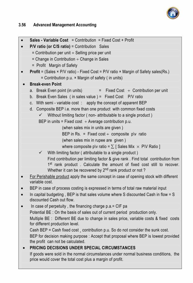
Advanced Management Accounting 3.56
• Sales - Variable Cost = Contribution = Fixed Cost + Profit • P/V ratio (or C/S ratio) = Contribution � Sales = Contribution per unit ÷ Selling price per unit = Change in Contribution ÷ Change in Sales = Profit � Margin of Safety • Profit = (Sales × P/V ratio) - Fixed Cost = P/V ratio × Margin of Safety sales(Rs.) = Contribution p.u. × Margin of safety ( in units) • Break-even Point
a. Break Even point (in units) = Fixed Cost ÷ Contribution per unit b. Break Even Sales ( in sales value ) = Fixed Cost � P/V ratio c. With semi - variable cost : apply the concept of apparent BEP d. Composite BEP i.e. more than one product with common fixed costs
Without limiting factor ( non- attributable to a single product ) BEP in units = Fixed cost ÷ Average contribution p.u. (when sales mix in units are given ) BEP in Rs. = Fixed cost ÷ composite p\v ratio (when sales mix in rupee are given ) where composite p\v ratio = ∑ [ Sales Mix × P\V Ratio ]
With limiting factor ( attributable to a single product ) Find contribution per limiting factor & give rank . Find total contribution from
1st rank product . Calculate the amount of fixed cost still to recover. Whether it can be recovered by 2nd rank product or not ?
• For Perishable product apply the same concept in case of opening stock with different variable cost.
• BEP in case of process costing is expressed in terms of total raw material input • In capital budgeting , BEP is that sales volume where S discounted Cash in flow = S
discounted Cash out flow. • In case of perpetuity , the financing charge p.a.= CIF pa Potential BE : On the basis of sales out of current period production only. Multiple BE : Different BE due to change in sales price, variable costs & fixed costs
for different production level. Cash BEP = Cash fixed cost ¸ contribution p.u. So do not consider the sunk cost. BEP for decision making purpose : Accept that proposal where BEP is lowest provided
the profit can not be calculated. • PRICING DECISIONS UNDER SPECIAL CIRCUMSTANCES
If goods were sold in the normal circumstances under normal business conditions, the price would cover the total cost plus a margin of profit.

CVP Analysis and Decision Making 3.57
The problem of pricing can be summarised under three heads: Pricing in periods of recession, Differential selling prices, and Acceptance of an offer and submission of a tender.
Pricing in periods of recession : Sell its articles at a price less than the total cost but above the marginal cost for a limited period.
Differential selling prices: Which is above, the marginal cost but below the total cost is resorted to in order to absorb surplus capacity.
• MAKE OR BUY DECISION Very often management is faced with the problem as to whether a part should be
manufactured or it should be purchased from outside market. Under such circumstances two factors are to be considered:
whether surplus capacity is available, and the marginal cost.
• SHUT DOWN OR CONTINUE DECISION A firm to temporarily close down the factory due to trade recession with a view to
reopening it in the future. In such cases, the decision should be based on the marginal cost analysis.
Shut down point = Total Shut
Contributifixed cost down
on per unit– costs
• EXPORT V/s LOCAL SALE DECISION When the firm is catering to the needs of the local market and surplus capacity is still
available, it may think of utilising the same to meet export orders at price lower than that prevailing in the local market.
• PRICE-MIX DECISION When a firm can produce two or more products from the same production facilities and
the demand of each product is affected by the change in their prices, the management may have to choose price mix which will give the maximum profit, particularly when the production capacity is limited.
SELF-EXAMINATION QUESTIONS 1. Is there any relationship between selling price and cost? 2. What are the items which the selling price should cover in different circumstances? 3. What are the advantages of selling above marginal cost but below total cost? 4. Is it justifiable to sell at a price below marginal cost any time? Mention the circumstances
in which it is justifiable? 5. What are the two ways in which differential selling price can be used?

Advanced Management Accounting 3.58
6. State the considerations which a firm has to give in (a) acceptance of an offer and (b) submission of a tender.
7. State what type of cost analysis is useful in taking managerial decisions in the following cases: (a) Make or Buy (b) Retain or Replace a machine (c) Shut down or continue (d) Export sale vs. Local sale (e) Change vs. Status quo (f) Expand vs. Contract.
8. A company produces four articles. Machine time is valuable due to heavy power cut imposed by the Government. Show which product should be produced so that the profit earned is the highest by utilising the scarce machine time.
9. A firm is desirous of replacing hand operation by machine operation to produce at faster rate. State how cost information will be useful in taking a decision.
10. Summarise the various factors to be considered in making recommendations for managerial decisions.
11. Ramesh of Agra presently operates its plant at 80% of the normal capacity to manufacture a product only to meet the demand of Government of Tamil Nadu under a rate contract. He supplies the product for Rs. 4,00,000 and earns a profit margin of 20% on sales realisations. Direct cost per unit is constant.
The indirect costs as per his budget projections are:
Indirect 20,000 units 22,500 units 25,000 units
costs (80% capacity) (90% capacity) (100% capacity)
Rs. Rs. Rs. Variable 80,000 90,000 1,00,000 Semi-variable 40,000 42,500 45,000 Fixed 80,000 80,000 80,000
He has received an export order for the product equal to 20% of its present operations. Additional packing charges on this order will be Rs. 1,000. Arrive at the price to be quoted for the export order to give him a profit margin of 10% on the export price. 12. The relevant data of X Ltd. for its three products A, B and C are as under; Product A B C
Direct material (Rs./Unit) 260 300 250 Direct labour (Rs./Unit) 130 270 260

CVP Analysis and Decision Making 3.59
Variable overheads (Rs./Unit) 110 230 180 Selling price (Rs./Unit) 860 1,040 930 Machine hours required (Per Unit) 12 6 3
The estimated fixed overheads at four different levels of 3,600; 6,000; 8,400 and 10,800 machine hours are Rs. 1,00,000; Rs. 1,50,000; Rs. 2,20,000 and Rs. 3,00,000 respectively. The maximum demand of A, B and C in a cost period are 500; 300 and 1,800 units respectively. You are required to find out (i) the most profitable product mix at each level and (ii) the level of activity where the profit would be maximum.
13. A company produces three products from an imported material. The Cost Structure per unit of the products are as under :
Product A B C
Rs. Rs. Rs.
Sales value 200 300 25 Direct material 50 80 60 Direct wages Rs. 6 per hour 60 120 108 Variable overheads 30 60 54
Out of Direct material 80% is Imported material @ Rs. 10 per kg. Prepare a statement showing comparative profitability of the three products under the following scenarios : (i) Imported material is in restricted supply. (ii) Production capacity is limiting factor. (iii) When maximum sales potential of products A and B are 1,000 units each and that of
product ‘C’ is 500 units for specific requirements, availability of imported material is restricted to 10,000 kgs. per month, how the profit could be maximised?
14. A machine manufactures 10,000 units of a part at a total cost of Rs. 21 of which Rs. 18 is variable. This part is readily available in the market at Rs. 19 per unit.
If this part is puchased from the market then the machine can either be utilised to manufacture a component in same quantity contributing Rs. 2 per component or it can be hired out at Rs. 21,000.
Recommend which of the alternative is profitable? ANSWERS TO SELF EXAMINATION QUESTIONS
1. In normal market conditions the answer is yes. But non-cost items also should be given due consideration.

Advanced Management Accounting 3.60
2. In normal periods, the prices should cover total cost. During recession, it is justifiable to continue if the prices cover marginal cost. In extra ordinary circumstances selling at a price below marginal cost may be justified for a limited period.
3. (a) skilled employees can be retained. (b) market is not lost. (c) plants and machinery do not become obsolescent. 4. (a) If goods are perishable in nature. (b) If stocks are excessive. (c) To popularise a new product. 5. (a) Dumping in export market by supplying the same product at lower price. (b) Selling a new product at a price which is less than the total cost but greater than
marginal cost. 6. Differential cost and differential revenue should be analysed. 7. (a) Use marginal cost analysis. (b) Use total differential cost analysis. (c) Consider additional fixed expenses incurred in shut down. (d) Utilisation of surplus capacity is the main consideration. (e) A detailed profitability analysis should be made. (f) Contribution analysis and the fixed expenses saved should be compared. 8. The key factor in this problem is machine time. Express the contribution as percentage of
the machine time. The product, which gives the highest contribution for key factor should be produced.
9. Make a total cost analysis and the interest on capital should be given due consideration. 10. (a) Marginal contribution. (b) Additional fixed expenses to be incurred. (c) Whether demand is inelastic and the price is stable. (d) Non-cost considerations should also be taken into account. 11. Export price to be quoted is Rs. 12.50 per unit. 12. (i) Most profitable product mix at each level is : Different levels (M/c Hrs) 3,600 6,000 8,400 10,800 Product mix C 1,200 1,800 1,800 1,800

CVP Analysis and Decision Making 3.61
units units units units B — 100 300 300 — units units units A — — 100 300 units units
(ii) The level of activity where the profit would be maximum: At 8,400 machine hours, level of capacity, the company would earn maximum profit i.e., Rs. 3,20,000.
13. (i) A is profitable (ii) A is profitable (iii) Product A B C
No. of units 1,00,000 562 500 Maximum profit (Rs.) 60,000 22,480 14,000
14. 3rd alternative i.e. 10,000 units of the products are purchased from outside and the maximum time is hired out at Rs. 21,000.

4 Pricing Decisions
LEARNING OBJECTIVES : After studying this unit you will be able to : • Understand and differentiate between different methods of Pricing the product. • Comment on the Pricing policy of the company • Understand the theory of Pricing under different • Appreciate the different strategies of pricing followed by the company and their
objectives. • Understand the meaning and applicability of Pareto Analysis.
4.1 INTRODUCTION A pricing decision is one of the most crucial & difficult decision that a firm has to make. Such a decision affects the long term life of any profit oriented enterprise. Accounting information is often an important input to pricing decisions. Most firms needs to make decision about setting or accepting selling prices for their products or services. In some firms selling prices are derived directly from cost information by estimating future products cost & adding a suitable profit margin. In others an established market price is accepted. Fundamentally, in pricing decision the management must first decide on its pricing goal and then set the base price for goods or services. After this the firm may design its pricing strategies. In this chapter we are going to discuss pricing of a finished product, the various types of pricing strategies and application of Pareto analysis. 4.2 THEORY OF PRICE The basic approach in most of the micro-economic theory (theory of the individual firm and its relation to other firms) defines the term optimum price as that price which yields the maximum profits (excess of total revenues over total costs). Thus the basic assumption of the pricing theory is that the firm’s main objective is to maximise its profits. It also assumes that the firm takes into consideration the position of demand and cost functions and that the firm produces one product.

Advanced Management Accounting 4.2
If a firm sell unlimited number of units, the total revenue line will be a straight line arrived at by TR= mx. where, TR = Total revenue line m = quantity of units sold x = price per unit. In most of the market situations, however, additional units can be sold by reducing the price. This means that although the total sales revenue will increase as more and more units are sold, the increase in total revenue will decline gradually as sales increases. Consider the following example: A firm’s pricing of a product is as under:
20 units @ Rs.4 per unit. 21 units @ Rs.3.90 per unit. 22 units @ Rs.3.80 per unit. The sales figures can be summarised as under:
Quantity Price Sale revenue Addition to total
revenue
Rs. Rs. Rs.
20 4.00 80.00 — 21 3.90 81.90 1.90 22 3.80 83.60 1.70
The reduction in the price of each additional unit reflects a gradual reduction in the steepness of the total revenue curve as shown in the diagram given on next page. The total cost curve will however, register an increase in the steepness because as the volume increases, the cost also increases because of the difficulty of expanding output with a given productive resources. The slope of the total revenue and total cost curves due to the addition of one unit will be equal to the increase in total revenue. This is the point where there will be no profit increase due to increase of one unit of output. In the figure [Fig. No. (1)], the situation has been depicted at point Z, where the gap between the total cost line and total revenue is the maximum, thus Z is the point of optimum volume. Any attempt to increase the volume beyond this point will reduce the profit because the incremental cost will be more than the incremental revenue. These relations are expressed in terms of marginal revenue and marginal cost. Marginal revenue, is the increase in total revenue that results from the sale of one additional unit. In the example given above, the marginal revenue of increasing one unit from 20 units to 21 units is

Pricing Decisions 4.3
Rs.1.90. Marginal cost is the increase in total cost that result from the production of one additional unit.
Figure 1
4.2.1 Pricing under different market structures : The determination of optimal price can be considered under the following market structures: (a) Pure competition: Under pure competition a firm has no pricing policy of its own as it has to accept the prevalent market price and at this price, it can sell all of its production if it so desires. But at any higher price it can sell nothing. There is no control over market price which will equate the quantities available with the quantities which the buyers are willing to buy. The firm has to take a decision in favour of the quantity to sell. The firm can continue to produce so long as its marginal cost is less than or equal to its selling price, Upto the point at which the marginal cost is equal to price, increase in output will add to revenue and thereafter the increase will add to cost. (b) Monopoly: It is a business situation which is characterised by: (i) one seller of a particular good or service (ii) competition from the producers of substitutes is almost insignificant.
4.3 PRICING POLICY The pricing policy plays an important role in a business because the long run survival of a business depends upon the firm’s ability to increase its sales and device the maximum profit from the existing and new capital investment. Although cost is an important aspect of pricing, consumer demand and competitive environment are frequently far more significant in pricing decisions. Thus costs alone do not determine prices. Cost is only one of the many complex factors which determine prices. There must however, be some margin in prices over total cost if capital is to be unimpaired and production maximised by the utilisation of internal surplus.

Advanced Management Accounting 4.4
The cost plus pricing method though common is not the best method because it ignores demand and fails to adequately reflect competition. The pricing policy and the relative price structure should: (a) provide an incentive to producer for adopting improved technology and maximising
production; (b) encourage optimum utilisation of resources; (c) work towards better balance between demand and supply; (d) promote exports; and (e) avoid adverse effects on the rest of the economy. Due to above characteristics, a monopolist can raise the price of its products without frightening away all his customers. How much he can raise from his customers, depends upon the elasticity of demand for his particular product. Under monopolistic condition, consumers may buy more at a lower price than at higher price. The profit can be maximised by equating marginal revenue with marginal cost. This cost be seen from the following diagram.
Figure 2
The point at which MR and MC curves meet will determine the price level. So the price will be BC and output to be manufactured will be OB. The firm may either fix output OB and leave the price to be fixed at BC or vice versa. There is, however, no protection for the existing firms from the entry of substitute firms (many sellers of similar but not necessary identical products) in the market. (c) Monopolistic competition: We saw that substitute firms who sell similar products enter the market and because of differentiation of products by sellers, monopolistic competition

Pricing Decisions 4.5
arises. Since there is limit to the growth of competitors the excess profits earned by monopolistic situation attracts new competition. This will have a long-run effect on the excess profits which will tend to diminish because of the price competition with close substitutes. The company will, however, have to compare marginal cost and marginal revenue in maximising its profits. (d) Oligopoly: If in a market there are a few large sellers occupying a major share of the market, the situation is called oligopoly. If the oligopolistic seller finds that his competitors also increase their prices with his decision to increase or decrease their prices with his decision to reduce, his revenue curve will have the same shape as that of the market as a whole. If the competitors, however, do not follow suit, the shift in the sales will be sensitive. If one seller increases his price while the others do not, the consumers will start buying from the competitors and the sales of the seller who increased his price will start buying from the competitors and the sales of the seller who increased his price will start falling off. Thus each firm will study the potential reaction before increasing or decreasing the selling price.
4.4 PRINCIPLES OF PRODUCT PRICING As already stated cost should not be considered as an important determinant of price. The tendency should be to lower the price in such a way so as to choose a right combination of price and output to maximise profits. The important determinants of price, therefore, are competitive situations prevailing in the market and elasticities. Taking the standard products into consideration, the pricing principles are much the same whether the product is a new one or the one already well established in the market. However the environmental situation and information base are different. Illustration A small scale manufacturer produces an article at the operated capacity of 10,000 units while the normal capacity of his plant is 14,000 units. Working at a profit margin of 20% on sales realisation, he has formulated his budget as under: Units 10,000 14,000 Rs. Rs. Sales realisation 2,00,000 2,80,000 Variable overheads 50,000 70,000 Semi-variable overheads 20,000 22,000 Fixed overheads 40,000 40, 000 He gets an order for a quantity equivalent to 20% of the operated capacity and even on this additional production profit margin is desired at the same percentage on sales realisation as for production to operated capacity. Assuming prime cost is constant per unit of production, what should be the minimum price to realise this objective?

Advanced Management Accounting 4.6
Solution Working Notes: (i) Computation of prime cost: Rs. Rs. The profit margin is 20% on sale Therefore, cost of sale, 80% of Rs. 2 lakhs 1,60,000 Variable overheads 50,000 Semi-variable overheads 20,000 Fixed overheads 40,000 1,10,000 Prime cost 50,000 (ii) Since an additional production of 4,000 units requires an increase of Rs. 2,000 in semi-
variable expenses, an additional production of 2,000 units will require an increase of Rs. 1,000 in semi-variable expense.
Computation of differential cost of production of 2,000 additional units for determining minimum price
Units 10,000 12,000 Differential cost for 2,000 units Rs. Rs. Rs. Prime cost 50,000 60,000 10,000 Variable overheads 50,000 60,000 10,000 Semi-variable overheads 20,000 21,000 1,000 Fixed overheads 40,000 40,000 — 1,60,000 1,81,000 21,000 The differential cost for an excess production of 2,000 units over the operated capacity is Rs. 21,000 i.e. Rs. 10.50 per unit. Profit margin required 20% on sale i.e. 25% on cost. Hence the minimum selling price = Rs. 10.50 + Rs. 2.625 = Rs. 13.125
4.5 NEW PRODUCT PRICING The pricing of new product poses a bigger problem because of the uncertainty involved in the estimation of their demand. In order to overcome this difficulty experimental sales are conducted in different markets using different prices to see which price is suitable. A company may, for example, choose three different markets and by using the same amount of sales promotional activities, ascertain what is the right price. In such circumstances, it may even prove that the highest price yielding the largest unit contributory margin need not necessarily maximise the profits. A lower price may well go to maximise the profits.

Pricing Decisions 4.7
Example A company choose three prices to be charged in three different markets and it can be seen from the figures given below that the intermediate price maximises profits.
Particulars Price Price Price
Selling price per unit Rs. 1.20 Rs. 1.50 Rs. 1.80 Estimated sales (units) 8,000 6,000 3,000 Rs. Rs. Rs. Sales revenue : (A) 9,600 9,000 5,400 Costs: Manufacturing costs 5,200 3,900 1,950 Selling expenses 1,000 500 450 Fixed expenses 1,500 1,500 1,200 Total : (B) 7,700 5,900 3,600 Profit : {(A) – (B)} 1,900 3,100 1,800
4.6. PRICING OF FINISHED PRODUCT 4.6.1 Cost plus pricing : In many business the common method of price determining is to estimate the cost of product & fix a margin of profit.. The term ‘cost’ here means full cost at current output and wage levels since these are regarded as most relevant in price determination .In arriving at cost of production, it is necessary to determine the size of the unit whose products are to be costed and priced. An individual manufacturer may take his cost of production into account and arrive at a price at which the products are to be sold in the concerned region. A manufacturer having several factories all over the country may determine the weighted average cost of each of the factories and include the same in his computations so as to arrive at a uniform price for the country as a whole, e.g., if prices are to be fixed by a statutory authority, like the Tariff Commissions; weighted average price is also taken into account if large number of factories are owned by one manufacturer. The price may also be fixed after taking into account the cost of a representative unit which may fall within the range of lowest cost unit and the highest cost unit. Alternatively, the factories may be classified into (i) small size factories, (ii) medium size factories, and (iii) large size factories. The cost of medium size factories can be taken into account if this group forms the greater part of the industry. Where however, the units in an industry are very large as in the case of textile industry for example, some representative sample has to be taken. The sample should be of economic size and also be of representative of the conditions of the different regions.. The demand of the product and the cost of the marginal unit may have to be

Advanced Management Accounting 4.8
taken into account in fixing the price so that the marginal units are not driven out of the market. In order to frame a price policy, one of the element that should receive consideration is the determination of normal capacity. Normal capacity is the utilisation of plant that is necessary to meet the average commercial demand over a period of time, long enough to level out peaks which come with seasonal and cyclical variations. The following chart illustrates the major relationships involved.
Operation interruptions Idle Capacity
Maximum Practical Capacity based Theoretical Plant on normal sales Capacity Capacity expectancy
Price determination should normally be based on the level of production and capacity utilisation likely to be achieved. Any assumption of low utilisation may result in over estimating the cost. Conversely, a high utilisation assumption may result in under estimating the cost. It is, therefore, desirable that the level of production and capacity utilisation which are likely to apply, say in the next three years should be arrived at with utmost care on realistic basis keeping in view not only the past performance but also the future demand. A uniform system of costing should also be devised and introduced in each industry for the fixation of price. If a firm wants to survive and stay in business, it has to maintain its fixed capital intact so that its fixed assets may be replaced at the end of their useful working life out of the funds generated from profits retained in the business. In a period of relatively stable price levels, depreciation based on historical cost of fixed assets would perhaps be adequate for achieving this object. In periods when the price level is continuously changing, the firm may not be left with adequate funds generated out of accumulated depreciation at the end of the life of the plant to replace the plant at a higher price. Hence depreciation should be properly included as a part of cost so as to leave sufficient profits for aseet replacement. Advantages : 1. Fair method:It is a fair method of price fixation. The business executives are convinced
that the price fixed will cover the cost. 2. Assured Profit: If price is greater than cost, the risk is covered. This is true when normal
expected capacity basis of cost estimation is used. 3. Reduced risks and uncertainties: A decision maker has to take decisions in the face of
many uncertainties. He may accept a pricing formula that seems reasonable for reducing uncertainty.
4. Considers market factors: This sort of pricing does not mean that market forces are ignored. The mark up added to the cost to make a price reflect the well established customs of trade, which guide the price fixer towards a competitive price.

Pricing Decisions 4.9
Disadvantages : 1. Ignores demand: It ignores demand. It fails to take into account the buyers’ needs and
willingness to pay which govern the sales volume obtainable at each series of prices. 2. Ignores competition: It fails to reflect competition adequately. 3. Arbitrary cost allocation: It takes for granted that the costs have been estimated with
exact accuracy which is not often true particularly in multi-product firms because the common costs are allocated arbitrarily.
4. Ignores opportunity cost: For many decisions incremental costs rather than full costs play a vital role in pricing. This aspect is ignored.
5. Price-Volume relationships: Since the fixed overheads are apportioned on the basis of volume of production, the cost will be more if a sales volume is less and cost will be less if sales volume is more. The increase or decrease in sales volume again is dependent of price. Thus it is a vicious circle–cost plus mark up is price based on sales volume and sales volume is based on price.
Illustration Prompt Printers Ltd., uses a scheme of pricing based on cost plus. All the overheads are charged, based on direct labour and based on the total cost arrived at, the selling price is fixed. The following figures are obtained from the Annual Budget for 1998 prepared by the company: Rs. Sales 10,00,000 Direct material 1,80,000 Direct labour 3,20,000 Factory superintendent’s salary 30,000 Commission paid on sales (5%) 50,000 Foreman’s salaries 60,000 Insurance 10,000 Advertisement 20,000 Depreciation on assets 30,000 Administration expenses 90,000 Variable factory costs : Repairs and maintenance 60,000 Tools consumed 40,000 Miscellaneous supplies 10,000

Advanced Management Accounting 4.10
The company has submitted a tender quoting Rs. 10,000 on a large order with a cost of Rs. 1,800 Direct materials and Rs. 3,200 Direct labour. The customer strikes the business at Rs. 8,900 on a ‘take it or leave it’ basis. If the company accepts the order, the total sales for 1998 would be Rs. 10,08,900. The company is reluctant to accept the order as it would be against its policy of accepting an order below cost. Write a note to the Managing Director, recommending the acceptance of the order, substantiating your recommendation fully with supporting figures to explain that the price offered would not be below cost and a sizeable profit also would be made. Also comment on the pricing policy of the company. Solution To : Managing Director From : Management Accountant Date : ..........
Subject : Additional order The additional order for which the company has submitted a tender quoting Rs. 10,000/and for which the customer has offered to strike the business at Rs. 8,900/- on a ‘take it or leave it’ basis and as the company is reluctant to accept the order as it would be against its policy of accepting an order below cost, the following is submitted for consideration of the Managing Director with the recommendation that the acceptance of the order will be profitable to the company as is substantiated by the following figures: At present the company determines the sales value as follows : Rs. Rs. Direct material 1,80,000 Direct labour 3,20,000 Variable overheads (Repairs and Maintenance, Tools consumed Misc. supplies and sales commission) 1,60,000 Fixed overhead (all other expenses) 2,40,000 4,00,000 Total cost 9,00,000 Profit 1,00,000 Sales 10,00,000 While applying overhead rate, the company does not distinguish between variable and fixed overheads. Overhead, as can be seen, is charged at 125% of direct labour and profit at 1/9 of total cost. On the same basis, the quotation price has been submitted as follows: Rs. Direct material 1,800 Direct labour 3,200

Pricing Decisions 4.11
Overhead (125% of direct labour) 4,000 Total cost 9,000 Profit 1/9 of total cost 1,000 Tender price 10,000 But this is an additional activity as the total sales after the acceptance of the order would be Rs. 10,08,900. To meet this order, only the variable overheads will be incurred as fixed overheads are absorbed by normal production. Therefore, the revised figures are : Rs. Rs. Price offered 8,900 Direct material 1,800 Direct labour 3,200 Variable overhead excluding sales commission 1,100 Sales commission @ 5% 445 6,545 Profit 2,355 It can be seen from the above that Rs. 8,900 price offered by the customer is well above the incremental cost of the additional order and the profit is above 1/3 of cost, much more than 1/9 of cost. Hence the company should accept the order. In making this recommendation, it has been assumed that the existing sales will remain unaffected by the acceptance of this order. Comments on the pricing policy of the company When overheads are capable of being distinguished as variable and fixed, it is wrong to club them together and charge overheads indiscriminately as a percentage of direct labour. Cost plus, as a basis of pricing, is allright for normal activity; but for incremental activity, the relevant cost is only the marginal cost and the profit on marginal activity, is normally greater than that of the original activity. Taking the whole cost and basing the price on cost plus will be misleading. It will result in loosing valuable profit opportunity for earning an additional profit. Illustration Chum Chum Ltd. is about to introduce a new product with the following estimates : Price per unit Demand (in rupees) (in thousand units) 30–00 400 31–50 380 33–00 360 34–50 340 36–00 315 37–50 280 39–00 240

Advanced Management Accounting 4.12
Costs : Direct material Rs. 12 per unit Direct labour Rs. 3 per unit Variable overhead Rs. 3 per unit Selling expenses 10% on sales Fixed production overheads Rs. 14,40,000 Administration expenses Rs. 10,80,000 Judging from the estimates, determine the tentative price of the new product to earn maximum profit. Solution Chum–Chum Ltd. Statement for determining tentative price of the new product, from estimates, to earn maximum profit
Price Demand Sales Variable Contriubtion per unit (Rs.) (in lakhs of unit) revenue costs (in Rs. lakhs) (in Rs. lakhs) (in Rs. lakhs) (Rs. 18 p.u. + 10% of selling price) (a) (b) (c) (d) (c–d) 30-00 4.00 120.00 84.00 36.00 31-50 3.80 119.70 80.37 39.33 33-00 3.60 118.80 76.68 42.12 34-50 3.40 117.30 72.93 44.37 36-00 3.15 113.40 68.04 45.36 37-50 2.80 105.00 60.90 44.10 39-00 2.40 93.60 52.56 41.04
The tentative price of the new product should be Rs. 36 per unit. At this price the profit of Chum-Chum Ltd. is maximum, the maximum profit of the concern comes to Rs. 20,16,000 (Refer to working note). Working note : Maximum profit = Maximum contribution – {Fixed production overhead + Administration expenses} = Rs. 45,36,000 – {Rs. 14,40,000 + Rs. 10,80,000} = Rs. 20,16,000

Pricing Decisions 4.13
4.6.2 Rate of Return Pricing : Determination of return on capital employed is one of the most crucial aspect of price fixation process. In this process instead of arbitrarily adding a percentage on cost for profit, the firm determines an average mark up on cost necessary to produce a desired rate of return on its investment. Under this method three issues arise: (a) The basis on which the capital employed is computed. (b) Which items should be covered in the return on capital. (c) What rate of return can be regarded as fair? The rate of return to be earned by the firm or industry must depend on the risk involved.., The desirability of earning adequate profits for the purpose of ploughing back into business should be kept in mind. It would be correct to assume that allowing the industry to earn adequate return on the capital employed would attract additional capital and increase the number of factories and production of all commodity which must ultimately lead to competition and reduction in costs and prices. Illustration Electromatic Excellers Ltd. specialises in the manufacture of novel transistors. They have recently developed a technology to design a new radio transistor capable of being used as an emergency lamp also. They are quite confident of selling all of the 8,000 units that they would be making in a year. The capital equipment that would be required will cost Rs. 25 lakhs. It will have an economic life of 4 years and no significant terminal salvage value. During each of the first four years promotional expenses are planned as under:
Year 1 2 3 4
Advertisement (Rs.) 1,00,000 75,000 60,000 30,000 Other expenses (Rs.) 50,000 75,000 90,000 1,20,000
Variable costs of producing and selling the unit would be Rs. 250 per unit. Additional fixed operating costs incurred because of this new product are budgeted at Rs. 75,000 per year. The company’s profit goals call for a discounted rate of return of 15% after taxes on investments on new products. The income tax rate on an average works out to 40%. You can assume that the straight line method of depreciation will be used for tax and reporting. Work out an initial selling price per unit of the product that may be fixed for obtaining the desired rate of return on investment. Present value of annuity of Re. 1 received or paid in a steady stream throughout 4 years in the future at 15% is 3.0079.

Advanced Management Accounting 4.14
Solution Determination of initial selling price Let the selling price be Rs. X Sales value : Rs. 8,000 X Annual cash costs are : Rs. Variable cost : 8,000 units × Rs. 250 20,00,000 Advertisement and other expenses 1,50,000 Additional fixed costs 75,000 Total cash cost 22,25,000
Depreciation per annum = Rs. , ,25 00 0004
= Rs. 6,25,000
Profit for taxation : Rs. 8,000 × Rs. X – (Rs. 22,25,000 + Rs. 6,25,000) = Rs. 8,000 X – Rs. 28,50,000 Tax at 40% on profit : 40% of {Rs. 8,000 X – Rs. 28,50,000} = Rs. 3,200 X – Rs. 11,40,000 Total annual cash outflow : Rs. 22,25,000 + (Rs. 3,200 X – Rs. 11,40,000) = Rs. 3,200 X – Rs. 10,85,000 Net annual cash inflow : Rs. 8,000 X – (Rs. 3,200 X + Rs. 10,85,000) = Rs. 4,800 X – Rs. 10,85,000 Now, present value of initial cash outflow = Present value of cash inflow or Rs. 25,00,000 = (Rs. 4,800 X – Rs. 10,85,000) × 3.0079 or X = Rs. 399.20 Hence selling price should be Rs. 399.20 per unit. Alternative Solution
Rs. Total variable costs per year 20,00,000 (8,000 × Rs. 250) Promotional costs per year 1,50,000 Fixed operating costs per year 75,000 22,25,000 Less: Income tax 40% (tax shield) 8,90,000 13,35,000

Pricing Decisions 4.15
Less: Tax saving on depreciation 2,50,000
× %40
4000,00,25.Rs
Net annual cash outflow 10,85,000 PV factor for 4 years @15% : is 3.0079 Therefore, present value of annual cash outflow : (Rs. 10,85,000 × 3.0079) 32,63,572 Initial investment 25,00,000 Present value of total outlay 57,63,572 Divide the present value of total outlay by PV factor to get required annual revenue after tax 19,16,145 (Rs. 57,63,572 ÷ 3.0079) Required annual revenue before tax : 31,93,575
×
60100145,16,19.Rs
Unit selling price : 399.20
units000,8575,93,31.Rs
4.6.3 Variable costs pricing : We have seen a number of decisions based on variable or marginal costing principle in the chapter of Marginal Costing. Pricing based on total costs is subjected to two limitations. They are : (a) the allocation of inter-departmental overheads is based on an arbitrary basis; and (b) the allocation overheads will require estimation of normal output which often cannot be
done precisely. In order to avoid these complications, variable costs which are considered as relevant costs are used for pricing, by adding a mark up to include fixed costs allocation also. 4.6.4 Competitive pricing : When a company sets its price mainly on the consideration of what its competitors are charging, its pricing policy under such a situation is called competitive pricing or competition-oriented pricing. It is not necessary under competitive pricing to charge the same price as charged by the concern’s competitors. But under such a pricing the concern may keep its prices lower or higher than its competitors by a certain percentage. Its own costs or demand may change, but the concern maintains its price because its competitors maintain their prices. Conversely, the concern will change its price when its competitors change their

Advanced Management Accounting 4.16
price, even if its own costs or demand have not altered. Different type of competitive pricing in vogue are as follows: (i) Going rate pricing (ii) Sealed bid pricing (i) Going rate pricing: It is a competitive pricing method under which a firm tries to keep its price at the average level charged by the industry. The use of such a practice of pricing is specially useful where it is difficult to measure costs. Adoption of going rate pricing will not only yield fair return but would be least disruptive for industry’s harmony. Going rate pricing primarily characterizes pricing practice in homogeneous product markets, The concern selling a homogeneous product in a highly competitive market has actually very little choice about the setting of its price. There is apt to be a market determined price for the product, which is not established by any single firm or clique of firms but through the collective interaction of buyers and sellers. The concern which is going to charge more than the going rate would attract virtually no customers. The concern should not charge less because it can dispose of its entire output at the going rate. Thus, under highly competitive conditions in a homogeneous product market (such as food, raw materials and textiles) the concern really has no pricing decision to make. The major challenge before such a concern is good cost control. Since promotion and personnel selling are not in the picture, the major marketing costs arise in physical distribution. In pure oligopoly, where a few large concerns dominate the industry, the concern also tends to charge the same price as is being charged by its competitors. Since there are only a few concerns, each firm is quite aware of others’ prices, and so are the buyers. This does not mean that the going price in an oligopoly market will be in practice indefinitely. It cannot, since industry costs and demand change over time. (ii) Sealed bid-pricing: Competitive pricing also dominates in those situations where firms compete on the basis of bids, such as original equipment manufacture and defence contract work. The bid is the firms offer price, and it is a prime example of pricing based on expectations of how competitors will price rather than on a rigid relation based on the concern’s own costs or demand. The objective of the firm in the bidding situation is to get the contract, and this means that it hopes to set its price lower than that set by any of the other bidding firms. But however the firm does not ordinarily set its price below a certain level. Even when it is anxious to get a contract in order to keep the plant busy, it can not quote price below marginal cost. On the other hand, if it raises its price above marginal cost, it increases its potential profit but reduces its chance of getting the contract. 4.6.5 Incremental pricing : Incremental pricing is used because it involves comparison of the impact of decisions on revenues and cost. If a pricing decision results in a greater increase in revenue than in costs, it is favourable. Such a decision is not merely confined to comparison of revenues and costs. It also permits that consideration being given to other objectives of the business. Thus profitability can be set as the matter of primary consideration and then the decision can be adjusted to bring it in consonance with the other decision of the business.

Pricing Decisions 4.17
The following points will be useful to show how this technique gives consideration to all repercussions of a decision.
1. Relevant cost analysis: This technique considers changes in costs rather than in average cost. Overhead allocations are irrelevant.
2. Product-Line relationship analysis: This technique necessitates consideration being given to possible complementary relations in demand. Sale of one product may lead to the sale of a complementary product. This overall effect on profitability has to be evaluated.
3. Opportunity cost analysis: The opportunity costs should be covered by the incremental revenue. A price which results in an incremental revenue which in turn merely covers the incremental costs is not sufficient. If the opportunity foregone is greater than incremental revenue, the decision is not sound.
4. Time factor analysis: The decision should take into account the short run and long run effects. A high price may increase its immediate profits but may lead to loss of revenue in the long run owing to competitors snatching the business.
5. CVP analysis: In fixing prices consideration should be given to price volume relationship. The responsiveness of the market to the price should be such that the volume is increased so that fuller utilisation of plant is achieved.
6. Risk analysis: Consideration should also be given to the evaluation of uncertainty. The decision taken should be able to maximise the expected value.
4.7 PRICING STRATEGIES
Pricing strategy is defined as a broad plan of action by which an organisation intends to reach its goal. Some illustrative strategies are:-
• Expanding product lines that enjoy substantial brand equity
• Offer quantity discounts to achieve increase in sales volume.
Since the right amount of volume has to be selected to optimise profit, sufficient promotional activities are necessary. In some cases it may even take a long time for the producer to establish. There are various type of pricing strategies which firm can adopt. Few of them are as follows :
4.7.1 Market-Entry strategies: While preparing to enter the market with a new product, management must decide whether to adopt a skimming or penetration pricing strategy.
(a) Skimming pricing: It is a policy of high prices during the early period of a product’s existence. This can be synchronised with high promotional expenditure and in the later years the prices can be gradually reduced. The reasons for following such a policy are :
(i) Inelastic demand: The demand is likely to be inelastic in the earlier stages till the product is established in the market.

Advanced Management Accounting 4.18
(ii) Sales boost: The charge of high price in the initial periods serves to skim the cream of the market that is relatively insensitive to price. The gradual reduction in price in the later year will tend to increase the sales.
(iii) Assured profit: This method is preferred in the beginning because in the initial periods when the demand for the product is not known the price covers the initial cost of production.
(iv) Cost revenue matching: High initial capital outlays, needed for manufacture, results in high cost of production. Added to this, the manufacturer has to incur huge promotional activities resulting in increased costs. High initial prices will be able to finance the cost of production particularly when uncertainties block the usual sources of capital.
(b) Penetration pricing : This policy is in favour of using a low price as the principal instrument for penetrating mass markets early. It is opposite to skimming price. The low price policy is introduced for the sake of long-term survival and profitability and hence it has to receive careful consideration before implementation
Penetrating pricing, means a pricing suitable for penetrating mass market as quickly as possible through lower price offers. This method is also used for pricing a new product. In order to popularise a new product penetrating pricing policy is used initially.
The company may not earn profit by resorting to this policy during the initial stage. Later on, the price may be increased as and when the demand picks up. The use of this policy by the existing concerns will discourage the new concerns to enter the market. This pricing policy is also known as “stay-out-pricing”.
The three circumstances in which penetrating pricing policy can be adopted are as under:
(i) Elastic demand: When demand of the product is elastic to price. In other words, the demand of the product increases when price is low.
(ii) Mass production: When there are substantial savings on large scale production. Here increase in demand is sustained by the adoption of low pricing policy.
(iii) Frighten competition: When there is threat of competition. The prices fixed at a low level act as an entry barrier to the prospective competitors.
4.7.2 Price discounts and differentials :
Distributors’ discounts : It means price deductions that systematically make the net price vary according to buyer’s position in the chain of distribution. These discounts are given to various distributors in the trade channel e.g., wholesalers, dealers and retailers. As these discounts create differential prices for different customers on the basis of marketing functions performed by them, so they are also called as functional discounts.

Pricing Decisions 4.19
l Various forms of Distributors discounts : Distributors discounts can be classified under the following three categories:
(i) Different net prices for different distributor levels: Net prices are commonly used as the device for quoting differential prices to distributors. A list of such prices is given to authorised dealers by manufacturers to facilitate their task of billing.
(ii) A uniform list price modified by a structure of discounts, each rate so determined is applied to a different level of distributor : This method is commonly used as it is easy to deal with its use in diverse trade channels. By merely varying the discounts it facilitates cyclical and seasonal adjustments in prices also. Its use helps in keeping actual prices a secret not only among distributors but also among competitors and customers. This method gives to manufacturers greater control over the realised margin of different categories of distributors.
(iii) A single discount combined with differing supplementary discounts to different levels of distributors: Supplementary discount gives clear cut picture about the trade channel structure or the suggested resale prices. These discounts reflect distributors cost at different stages and competition between different kinds of distributors. These discounts are often very elaborate and are in use due to tradition in the industry.
• Pre-requisites for determining Distributors’ Discounts: The economic function of distributors discounts is to induce different categories of distributors to perform nicely, their respective marketing functions. As such, to build up a discount structure on sound economic lines, it is essential to know about :
(i) The services to be performed by the distributors at different levels.
(ii) Knowledge about distributors’ operating costs.
(iii) Discount structure adopted by competitors.
(iv) Effect of discounts on distributor’s population.
(v) Costs of selling to different channels.
(vi) Availability of opportunities for market segmentation.
• Quantity discounts : Quantity discounts are price reductions related to the quantities purchased. It may take several forms. It may be related to the size of the order which is being measured in terms of physical units of a particular commodity. This is practicable where the commodities are homogeneous or identical in nature, or where they may be measured in terms of truck-loads.
However, this method is not applicable in the case of heterogeneous commodities as it is difficult to add them in terms of physical units or truck loads e.g. textile and drug industry. Quantity discounts are useful in the marketing of materials and supplies but are rarely used for marketing equipment and components.

Advanced Management Accounting 4.20
Objectives of quantity discounts: The main objective of quantity discounts is to reduce the number of small orders and thus avoid the high cost of servicing them.
Advantages: Quantity discount system enables the dealer to avail such discounts by buying larger lots. The economic buying by a dealer may enable him to charge lower prices from his customers thereby benefiting them. Finally, lower prices to customers may increase their demand for the commodities which in turn may enable the dealer to purchase larger quantities, reaping still greater discounts, and the manufacturer to reap economies of large-scale production. In some cases, discounts become a matter of trade custom.
Disadvantages: Dealers may find it cheaper to purchase their requirement of commodities from wholesalers, availing themselves of these quantity discounts than from the manufacturers directly. This is because the wholesalers may pass on some of their discount to the dealers. Such a practice may affect the image of the manufacturer in the minds of the dealers.
Cash Discounts : Cash discounts are price reductions based on promptness of payment. It is a convenient device to identify and overcome bad credit risks. In those trades where credit risk is high, the percentage of cash discount given is also high. If a buyer decides to purchase goods on credit, he has to pay a higher price by foregoing the cash discount.
Time differentials : Charging different prices on the basis of time is another kind of price discrimination. Under time differentials the objective of the seller is to take advantage of the fact that buyers demand elasticities vary over time. Time differentials can be classified under the following heads.
(i) Clock-time differentials: The price differentials are known as clock-time differentials when different prices are charged for the same service or commodity at different times within a 24 hour period. Common examples of these are, the differences between the day and night rates on trunk calls; difference between the rates charged in morning and regular shows in cinema houses.
(ii) Calendar-time differentials: Here price differences are based on a period longer than 24 hours. For example; seasonal price rate variations in the case of winter clothing or hotel accommodation at a hill station and a tourist resort. The main objective here is to exploit the time preferences of the buyers.
(iii) Geographical price differentials: It refers to price differentials based on buyers location. The objective here is to exploit the differences in transport-cost, due to the varying distances between the locations of the plants and customers.
(iv) Consumer category price differentials: Price discriminations is frequently practised according to consumer categories in the case of public utilities, e.g., electricity, transportation, etc. Electricity companies charge different rates for residential consumers and industrial consumers. The rates may also differ to domestic power, light and fan.
4.7.3 Price Discrimination : Price discrimination means charging different prices and it takes various forms according to whether the basis is customer, product, place or time. These are illustrated as under:

Pricing Decisions 4.21
(a) Price discrimination on the basis of customer: In this case, the same product is charged at different prices to different customers. It is, however, potentially disruptive of customer relations.
(b) Price discrimination based on product version: In this case, a slightly different product is charged at a different price regardless of its cost-price relationship. If, for example, a table with wooden top can be sold at Rs. 400, a table with sunmica top costing Rs. 175 extra is sold at Rs. 575. The higher premium in the latter case does not necessarily reflect the higher production cost.
(c) Price discrimination based on place: An example of this method is the seats in cinema theatre where the front seats are charged at lower rates than the back seats.
(d) Price discrimination based on time: An example of this method is the practice of giving off-season concession in sale of fans or refrigerators just after the summer season.
Price discrimination is possible if the following conditions are satisfied :
(a) the maker must be capable of being segmented for price discrimination;
(b) the customers should not be able to resell the product of the segment paying higher price; and
(c) the chance of competitors’ underselling in the segment of higher prices should not be possible.
4.7.4 Geographic Pricing Strategies : In pricing, a seller must consider the costs of shipping goods to the buyer. These costs grow in importance as freight becomes a larger part of total variable costs. Pricing policies may be established whereby the buyer pays all the freight expense, the seller bears the entire cost, or the seller and buyer share this expense. The strategy chosen can influence the geographic limits of a firm’s market, locations of its production facilities, sources of its raw materials, and its competitive strength in various geographic markets.
Point-of-Production Pricing : In a widely used geographic pricing strategy, the seller quotes the selling price at the point of production and the buyer selects the mode of transportation and pays all freight costs.
This method of pricing is referred as FOB factory pricing.
Uniform Delivered Pricing : Under uniform delivered pricing, the same delivered price is quoted to all buyers regardless of their locations.
Uniform delivered pricing is typically used where freight costs are a small part of the seller’s total cost. This strategy is also used by many retailers who believe “free” delivery is an additional service that strengthens their market position.
Zone-Delivered Pricing : Zone-delivered pricing divides a seller’s market into a limited number of broad geographic zones and then sets a uniform delivered price for each zone.

Advanced Management Accounting 4.22
Freight-Absorption Pricing : Under freight-absorption pricing, a manufacturer will quote to the customer a delivered price equal to its factory price plus the freight costs that would be charged by a competitive seller located near that customer.
4.8 PARETO ANALYSIS
Pareto Analysis is a rule that recommends focus on the most important aspects of the decision making in order to simplify the process of decision making. It is based on the 80 : 20 rule that was a phenomenon first observed by Vilfredo Pareto, a nineteenth century Italian economist. He noticed that 80% of the wealth of Milan was owned by 20% of its citizens. This phenomenon, or some kind of approximation of it say, (70 : 30 etc.) can be observed in many different business situations. The management can use it in a number of different circumstances to direct management attention to the key control mechanism or planning aspects. It helps to clearly establish top priorities and to identify both profitable and unprofitable targets.
4.8.1 Usefulness of Pareto Analysis : It provides the mechanism to control and direct effort by fact, not by emotions. It helps to clearly establish top priorities and to identify both profitable and unprofitable targets.
Pareto analysis is useful to:
• Prioritize problems, goals, and objectives Identify root causes .
• Select and define key quality improvement programs Select key customer relations and service programs Select key employee relations improvement programs.
• Select and define key performance improvement programs Maximize research and product development time.
• Verify operating procedures and manufacturing processes.
• Product or services sales and distribution.
• Allocate physical, financial and human resources.
4.8.2 Application of Pareto Analysis : Pareto analysis may be applicable in the presentation of Performance Indicators data through selection of representative process characteristics that truly determine or directly or indirectly influence or conform the desired quality or performance result or outcome. The Pareto Analysis is generally applicable to the following business situations :
(i) Pricing of a product :
• In the case of a firm dealing with multi products, it would not be possible for it to analyse cost-profit- price -volume relationships for all of them.
• In practice, in case of such firm approximately 20% of products may account for about 80% of total sales revenue. Pareto Anaysis is used for analysing the firm estimated sales revenues from various products and it might indicate that

Pricing Decisions 4.23
approximately 80% of its total sales revenue is earned from about 20% of its products.
• Such analysis helps the top management to delegate the pricing decision for approximately 80% of its products to the lower levels of management, thus freeing themselves to concentrate on the pricing decisions for products approximately 20% which are essential for the company’s survival.
• Thus, a firm can adopt more sophisticated pricing methods for small proportion of products that jointly accounts for approximately 80% of total sales revenue. For the remaining 80% of the products which account for 20% of total sales revenue the firm may use cost based pricing method.
(ii) Customer Profitability analysis:
• Instead of analysing products, customers can be analysed for their relative profitability to the organisation.
• Again it is often found that approximately 20% of customers generate 80% of the profit. There will always be some customers who are less profitable than others, just as some products are less profitable than others.
• Such an analysis is useful tool for evaluation of the portfolio of customer profile and decision making such as whether to continue serving a same customer group, what is the extent of promotion expenses to be incurred.
(iii) ABC analysis- Stock Control: Another application of Pareto analysis is in stock control where it may be found that only a few of the goods in stock make up most of the value. In practice approximately 20% of the total quantity of stock may account for about 80% of its value. The outcome of such analysis is that by concentrating on small proportion of stock items that jointly accounts for 80% of the total value, a firm may well be able to control most of monetary investment in stocks.
(iv) Application in Activity Based Costing: In Activity Based Costing it is often said that 20% of an organisation cost drivers are responsible for 80% of the total cost. By analysing, monitoring and controlling those cost drivers that cause most cost, a better control and understanding of overheads will be obtained.
(v) Quality Control :
• Pareto analysis seeks to discover from an analysis of defect report or customer complaints which “vital few” causes are responsible for most of the reported problems.
• Often, 80% of reported problems can usually be traced to 20% of the various underlying causes. By concentrating once efforts on rectifying the vital 20%, one can have the greatest immediate impact on product quality.

Advanced Management Accounting 4.24
• The Pareto Analysis indicates how frequently each type of failure (defect) occurs. The purpose of the analysis is to direct management attention to the area where the best returns can be achieved by solving most of quality problems, perhaps just with a single action.
Example
A Toy company performs a Pareto analysis, given a set of ‘defect types’ and frequencies of their occurrence. The sample data consists of information about 84 defective items. The items have been classified by their ‘defect types’ as follows:
Defect Types No. of Types
Cracks (due to mishandling of raw material) 10
Improper shapes 8
Incomplete 8
Surface scratches 53
Other (due to bad quality raw material) 5
Frequency table indicating the frequency of occurrence of defects in decreasing order of their occurrence will be as follows :
Defect type No. of items % Cummulative %
Surface scratches 53 63.1 63.1
Cracks 10 11.9 75
Improper shape 8 9.52 84.52
Incomplete 8 9.52 94.05
Other 5 5.95 100
The pareto chart is then constructed for defect type. For graphical construction of Pareto Chart the students may refer to recommended books on the subject.
The purpose of Pareto analysis in this example, is to direct attention to the area where best returns can be achieved by solving most of the quality problems, perhaps just with a single action. In this case, use of good quality raw material say plastic may solve 63% of problem and if raw material is handled properly at least 75% the problems may be overcome.

Pricing Decisions 4.25
SUMMARY • Pricing decisions should be made very carefully since they affect the long term
profitability of the concern. • There are various methods available for pricing of a finished product viz. cost plus
pricing, rate of return pricing, variable cost pricing, competitive pricing, incremental pricing et.al.
• Pricing of a new product is generally tough because of the uncertainty involved in the estimation of their demand.
• Pricing strategy is defined as a broad plan of action by which an organization intends to reach its goals.
• There are primarily two pricing strategies available namely Skimming pricing Strategy and Penetration Pricing Strategy.
• Pareto analysis is the rule that focuses on the most important aspect of decision making.
• It is based on the80:20 phenomenon, first observed by Vilfredo Pareto. • Activity Based Costing is the method of costing which involves identification of cost
drivers for various items of overheads.
SELF-EXAMINATION QUESTIONS 1. Fill in the blanks:
(a) There is no price policy in ........................ (b) If few sellers occupy a major share in the market, the situation is called
...................... (c) Charging a high price in the beginning of the product’s life cycle is known
as................. (d) Charging of low prices in the beginning of the life of a new product is known as
................... 2. State whether the following statements are true or false:
(a) Cost plus pricing does not take into account competition and demand. (b) When price reductions are introduced to increase sales revenue, the revenue line
will be a straight line. (c) Highest price yielding largest contributory margin need not necessarily maximise
profits. (d) In fixing selling prices, volume consideration should be taken into account so that
fuller utilisation of plant capacity is achieved. (e) A major consideration for skimming pricing is threat of competition.

Advanced Management Accounting 4.26
3. State whether the following statements are true or false: (a) Where a number of factories are owned by a company, weighted average cost can
be used for price fixation. (b) Price fixation is based on the total capacity of output which factory is capable of
manufacturing. (c) Survival and progress of a firm depend on its ability to maintain and replace,
whenever necessary, its fixed assets. (d) Depreciation should be allowed on replacement cost basis for price fixation.
4. Fill in the blanks : (a) Cost plus pricing ignores .................... and .................. (b) The rate of return to be earned by factory should cover the ............. involved in
business. (c) Price discrimination between various customers is ....................to customer
relations. (d) Pricing based on total cost is not considered accurate because of the difficulty
involved in........ 5. Discuss briefly the concept of skimming pricing policy. 6. ACE Ltd. has an inventory of 5.000 unit of a product left over from last year’ production.
This product is no longer in demand. It is possible to sell these at reduced prices through the normal distribution channels. The other alternative is ask someone to take them on “as is where is” basis. The latter alternative will cost the company Rs 5.000.
The company produced 2.40.000 units of the product last year, when the unit costs were as under:
Rs. Rs. Manufacturing cost :
Variable 6.00 Fixed 1.00 7.00 Selling & Distribution cost: Variable 3.00 Fixed 1.50 4.50 Total cost 11.50 Selling price per unit 14.00

Pricing Decisions 4.27
Required: Should the company scrap the items or sell them at a reduced price? If you suggest
the latter. What minimum price would you recommend ? 7. Somesh of Agra presently operates its plant at 80% of the normal capacity to
manufacture a product only to meet the demand of Government of Tamil Nadu under a rate contract.
He supplies the product for Rs. 4,00,000 and earns a profit margin of 20% on sale realisations.
Direct cost per unit is constant. The indirect costs as per his budget projections are:
Indirect costs 20,000 units 22,500 units 25,000 units ( 80% capacity) (90% capacity) (100% capacity) Rs. Rs. Rs. Variable 80,000 90.000 1,00,000 Semi-variable 40,000 42,500 45,000 Fixed 80,000 80,000 80,000 He has received an order for the product equal to 20% of its present operations. Additional packing charges on this order will be Rs. 1,000. Arrive at the price to be quoted for the export order to give him a profit margin of 10% on the export price. 8. What is Pareto Analysis. 9. Explain the application of Pareto Analysis in the following business situations :
(i) Stock Control (ii) Customer profitability (iii) Quality Control (iv) Pricing of a product.
ANSWERS TO SELF-EXAMINATION QUESTIONS 1. (a) pure competition, (b) oligopoly, (c) skimming price, (d) penetration price. 2. (a) True, (b) False, (c) True, (d) True, (e) False. 3. (a) It is only one of the factors, (b) False, (c) True, (d) Depends on actual circumstances.

Advanced Management Accounting 4.28
4. (a) Demand, competition, (b) risk, (c) disruptive, (d) determining cost where level of output changes. 6. If the company gets anything more than Rs. 2 per unit, then it is worthwhile to sell the
stock of 5,000 units & earn on additional contribution. 7. Price to be quoted Rs. 50,000 for the order of 4,000 units.

5 Budget & Budgetary Control
5.1 INTRODUCTION In your studies related to the previous stage of examinations, you were introduced to the concept of Budgeting and Budgetary Control. Having read that chapter you should be able to understand the following;
• The meaning of budgeting and budgetary control
• The objectives, advantages and disadvantages of budgeting and budgetary control
• The concept of functional budgets and their various types
• The difference between a fixed and a functional budget. In this chapter you shall further increase your understanding of the above mentioned and learn more about concepts related to identifying and using limiting factors for preparation of budgets, the relationship between strategic, operational and budgetary planning, the actual making of functional budgets from given data and other important budgetary tools like zero based budgeting and performance budgeting.
5.2 STRATEGIC PLANNING, BUDGETARY PLANNING AND OPERATIONAL PLANNING Planning is perhaps one of the most important tools in the hands of management to decide upon future course of action. It will be useful at this stage to distinguish in broad terms between three different types of planning:
• Strategic Planning;
• Budgetary Planning;
• Operational Planning. These three forms of planning are interrelated. The main distinction between them relates to their time span which may be short term, medium term or long-term. 5.2.1 Strategic Planning: Strategic planning is concerned with preparing long-term action plans to attain the organization’s objectives by considering the changes at horizon. 5.2.2 Budgetary Planning: Budgetary planning is mainly concerned with preparing the short to medium term plan of the organisation. It will be carried out within the framework of the

Advanced Management Accounting 5.2
strategic plan as already set. An organization’s annual budget is considered as an intermediary step towards achieving the strategic plan. 5.2.3 Operational Planning: It concerns with the short-term or day-to-day planning process. It plans the utilisation of resources and will be carried out within the framework of the budget. Each step in the operational planning process is an interim step towards achieving the budget.
5.3 THE PREPARATION OF BUDGETS The process of preparing and using budgets will differ from organisation to organisation. However, there are a number of key requirements in the design of a budgetary planning and control process. 5.3.1 Co-ordination: The budget committee: Budgets provide a means of co-ordination of the business as a whole. In the process of establishing budgets, the various factors like production capacity, sales possibilities, and procurement of material, labour, etc. are balanced and co-ordinates so that all the activities proceed according to the objective. For this purpose a budget committee is formed which includes all the departmental heads together to solve a common problem. The need for co-ordination in the planning process is immense. The interrelationship between the functional budgets (e.g. sales production, purchasing) means that one budget cannot be completed without reference to several to several others. 5.3.2 Participative budgeting: CIMA defines participative budgeting as: A budgeting system in which all budget committee members are given the opportunity to apply their own budgets in practice. This is known as ‘bottom-up budgeting’. It contrasts with imposed or top-down budgets where the ultimate budget holder does not have the opportunity to participating in the budgeting process. The advantages of participative budgeting are as follows:
• Improved quality of forecasts to use as the basis for the budget: Managers who are doing a job on a day-to-day basis are likely to have a better idea of what is achievable, what is likely to happen in the forthcoming period, local trading conditions, etc.
• Improved motivation: Budget holders are more likely to want to work to achieve a budget that they have been involved in setting themselves, rather than one that has been imposed on them from above.
• Better results: being the executor of the budget the applicant can control the costs better than any other manager.

Budget & Budgetary Control 5.3
5.3.3 The Budget Manual: Effective budgetary planning relies on the provision of adequate information to the individuals involved in the planning process. Many of these information needs are contained in the budget manual. A budget manual is a collection of documents that contains key information for those involved in the planning process. Typical contents could include the following: a) An introductory explanation of the budgetary planning and control process, including a
statement of the budgetary objective and desired results. b) A form of organisation chart to show who is responsible for the preparation of each
functional budget and the way in which the budgets are interrelated. c) A timetable for the preparation of each budget. This will prevent the formation of a
‘bottleneck’ with the late preparation of one budget holding up the preparation of all others.
d) Copies of all forms to be completed by those responsible for preparing budgets, with explanations concerning their completion.
e) A list of the organization’s account codes, with full explanations of how to use them. f) Information concerning key assumptions to be made by managers in their budgets, for
example the rate of inflation, key exchange rates, etc. 5.3.4 Identification of the principal budget factor: The principal budget factor is the factor that limits the activities of functional budgets of the organisation. The early identification of this factor is important in the budgetary planning process because it indicates which budget should be prepared first. In general sales volume is the principal budget factor. So sales budget must be prepared first, based on the available sales forecasts. All other budgets should then be linked to this. Alternatively, machine capacity may be limited for the forthcoming period and therefore machine capacity is the principal budget factor. In this case the production budget must be prepared first and all other budgets follows it. Failure to identify the principal budget factor at an early stage could lead to delays later on when managers realize that the targets they have been working with are not feasible. In case of one limiting factor, we shall need to apply the concept of Marginal costing. In this we initially allot the limiting resource on the basis of highest contribution per limiting factor. 5.3.5 How to identify the principle budget factor 1. in case of single product organisation 2. in case of multi product organisation

Advanced Management Accounting 5.4
5.3.5.1 In case of single product organisation Steps to follow (i) Identify the capacity of the production departments. Generally normal capacity is
consider for budget / estimation ( Ref Cost Accounting Standards 2, 3) (ii) Maximum production in adept. = normal capacity ÷ time p.u. (iii) Select the minimum production volume among the above results. The dept. producing
that result is known as bottleneck among the production department. (iv) Identify the sale or demand of the product. (v) Now by comparing the above 2 steps we can identify the principle budget factor. Explanation of Step-1: Capacity of a department is defined as facility available for work & generally expressed in terms of labour hour, machine hour or unit. There are 4 different expression of capacity. 1. Maximum capacity (Theoretical capacity) 2. Practical capacity 3. Normal capacity 4. Actual capacity Calculation 1. Maximum capacity = Maximum no. of days in a period ´ No. of workers ´ hrs/days. 2. Practical capacity = maximum capacity – Sunday & statutory holidays & normal
maintenance & idle time. 3. Normal capacity- it is the average of the last 3-year of normal performance if there is any
abnormal is any abnormal data don’t consider in the computing the average. 4. actual capacity : it can be determined only at the end of the period. So it has no
importance for preparation of budget. Illustration In a year, 15 workers are working in a dept. on a single shift basis. Statutory holidays in that year are 18. Normal maintenance requires 250 hrs./ p.m. The capacity utilization during last 5 years. 2000 30,000 Labour hour (LHR) 2001 38,000 “ “ 2002 31,000 “ “

Budget & Budgetary Control 5.5
2003 30,900 “ “ 2004 26,000 “ “ Calculate capacity of the organisation. Solution Maximum capacity = 365 days × 15 workers × 8 hrs p.day = 43,800 LHR Practical capacity = { 365- (52+18) days } × 15 workers × 8 hrs. p. day - 250 hrs p.m. ×12 = 32,400 LHR The capacity utilization during last 5 years. Years 2000 30,000 LHR 2001 38,000 “ (to high) 2002 31,000 “ 2003 30,900 “ 2004 26,000 “ (to low)
∴ Normal capacity of 2005 = (30,000 + 31,000 + 30,900 ) ÷ 3 = 30,633 LHR While preparing the budget we consider the normal capacity as budgeted production level
∴100% of budgeted capacity always implies the normal capacity. Explanation of Step- 2, 3 & 4. Illustration . There are 3 departments with different normal capacity & time required p.u. is given:
Machine Assembly Finishing (a) Capacity 1,2000 MHR. 8,000 LHR. 9,000 LHR (b) Time required/unit 4 MHR. 5 LHR. 3 LHR (c) Maximum production in a department 3,000 1,600 3,000 (a÷ b)
∴ Feasible production =1,600 units
∴ Assembly department is considered as bottleneck to the above production line. Illustration Solo products Ltd. manufactures and sells a single product and has estimated sales revenue of Rs.126 lakhs this year based on a 20 per cent profit on selling price.

Advanced Management Accounting 5.6
Each unit of the product requires 3 lbs of material P and 1½ lbs of material Q for manufacture as well as a processing time of 7 hours in the Machine shop and 2½ hours in the Assembly Section. Overheads are absorbed at a blanket rate of 33.3333% of Direct Labour. The factory works 5 days of 8 hours a week in a normal 52 weeks a year. On an average statutory holidays, leave and absenteeism and idle time amount to 96 hours, 80 hours and 64 hours respectively, in a year. The past performance (in Hours) of factory in last 3 yrs is as follows- Machine Shop Assembly shop In 2003 11,00,000 3,45,000 In 2004 10.30.000 3,20,000 In 2005 10,80,000 3,40,000 The other details are as under : Rs. Purchase price Material P 6 per lb Material Q 4 per lb Comprehensive Labour Rate Machine Shop 4 per hour Assembly 3.20 per hour No. of Employees Machine Shop 600 Assembly 180
Finished Goods Material P Material Q
Opening Stock 20,000 units 54,000 lbs 33,000 lbs Closing Stock (Estimated) ? 30,000 lbs 66,000 lbs
You are required to calculate the closing stock of finished goods: Solution (a) Working note-1 Computation of sale volume
Cost Sheet Rs. p.u. Rs. p.u. Material P: 3 lb@ 6 18 Q: 1 ½ lb @ 4 6 24 Labour 7 hrs. @ Rs. 4 28

Budget & Budgetary Control 5.7
Assembly 2.5 hrs. @ Rs. 3.2 8 36 Overhead 33 ½ of DL 12 Cost of production 72 Add: Mark up (25%) 18 (a) Sales 90 (b)Sales value Rs 126 lakhs No. of units sold (b�a) 1,40,000 Computation of principal budgeted factor (1) Sales/Demand 1,40,000 (2) Feasible production = Normal capacity ÷ time p.u.
Machine dept: 10, 70,000÷7 1, 52,857
Assembly dept.: 3.35,000÷2.5 1, 34,000
÷ Feasible production during this period 1, 34,000 units as Assembly department is the bottleneck. Computation of expected closing stock of finished goods Opening stock (units) 20,000 Add: estimated production (units) 1,34,000 Qty (units) 1,54,000 Less: demand (units) 1,40,000
∴Closing stock (units) 14,000 5.3.5.2 In case of multi product organisation 1. Sale / demand is the principle budget factor 2. Capacity is in short supply or limiting factor i.e. capacity requirement according to
demand is more than its supply a. Only one limiting factor b. More than one limiting factor 1. Sale / Demand is the principle budget factor Require sale mix = required contribution ÷ average contribution Average contribution = total contribution from all products ÷ total units

Advanced Management Accounting 5.8
Illustration P. H. Ltd. has specialised in the manufacture of three kinds of sub-assemblies required by the manufacturers of certain equipments. The current pattern of sales of sub-assemblies is in the ratio (in units) of 1 : 2 : 4 for sub-assemblies P, Q and R respectively. The sub-assemblies consist of the following components:
Sub-assembly Selling Requirement of components price Rs. Frame Part X Part Y Part Z
P 430 1 10 2 8 Q 500 1 2 14 10 R 600 1 6 10 2 Purchase Price (Rs.) 40 16 10 6
The direct labour hours required for the manufacture of each of the sub-assemblies are: Sub-assembly Skilled Hours Un-Skilled Hours P 4 4 Q 3 4 R 3 6 Wage rate per hour (Rs.) 6 5 The labourers work for 8 hours a day for 25 days a month. Variable overheads per sub-assembly are P Rs. 10, Q Rs. 8 R Rs. 7. Fixed overheads budget per month is an under: Rs. Production 15,80,000 Selling & Distribution 7,28,000 Administration 6,76,000 All fixed overheads are incurred evenly throughout the year. The target of profit for the current year is Rs. 120 lakhs before tax. The company has to plan to reduce the closing stock of sub-assemblies and components by 10 % as compared to the opening stock. Find the Sales in quantities

Budget & Budgetary Control 5.9
Solution Computation of variable cost per unit of 3 products
Items P Q R
Frame @ Rs. 40 40 40 40 Part- X 160 32 96 (10×16) (2×16) (6×16) Y 20 140 100 (2×10) (14×10) (10×10) Z 48 60 12 8×6 10×6 2×6 Wages –Skilled @ Rs. 6 24 18 18 Unskilled @ Rs. 5 20 20 30 Overhead 10 8 7 Variable cost 322 318 303
Note 2 Computation of Average Contribution Product SP VC Contribution SP mix Total contribution A b p/u (a-b) P 430 302 108 1 108 Q 500 318 182 2 364 R 600 303 297 4 1,188 7 1,660 Average contribution = Rs 237.14 Required profit p.m. Rs. 10, 00,000 Required fixed cost Rs. 29, 84,000 Required contribution Rs. 39, 84,000 Required sales = 39,84�000�(1,660/7) = 16,800 units Sales P 16,800×1/7 = 2,400 Q 16,800×2/7 = 4,800 R 16,800×4/7 = 9,600

Advanced Management Accounting 5.10
Capacity is in short supply or limiting factor i.e. capacity requirement according to demand is more than its supply : Only one limiting factor Illustration The sales, cost, selling price and processing time of three different herbal drinks produced by a company for the year just concluded are given below:
Product Strong Normal Mild Annual sales (no. of packs 250 gm) 6,000 5,000 1,000 Selling price (Rs./pack) 50 40 30 Unit cost (Rs../pack) 42 36 21 Processing time/ per pack (hrs) 1.5 1 2
The total processing hours available to the company is fully utilised for this sale. Fixed manufacturing overheads are fully absorbed in unit cost at rate of 200% of variable cost. For the coming year the demand for the three products has been estimated as under: Strong- 6,000 packs Normal- 6,000 packs Mild – 2,000 packs Considering that the selling prices are fixed and the processing time can be switched from one product line to another, calculate the best production programme for next operating year indicating the increase in net profit that will result. Solution Products Strong Normal Mild Total (a) Production & sales 6,000 5,000 1,000 Rs./unit Sales 50 40 30 Less: Variable cost (TC×1/3) 14 12 7 (b) Contribution 36 28 23 (c) Total contribution (Rs.) (a xb) 2,16,000 1,40,000 23,000 3,79,000 (d) Fixed cost p.u. (TC×2/3) (Rs.) 28 24 14 (e) Total fixed cost (a×d) (Rs.) 1,68,000 1,20,000 14,000 3,02,000 Profit 77,000 (f) MRs./unit 1.5 1.0 2.0 (g) Total processing time (a×f) 9,000 5,000 2,000 16,000 hr.

Budget & Budgetary Control 5.11
Capacity requirement or process time required in next year.
Product Demand Hr./ut Total hours. (a) (b) (a×b)
Strong 6,000 1.5 9,000 Normal 6,000 1.0 6,000 Mild 2,000 2.0 4,000 19,000 Less: Average 16,000 Shortage 3,000 Statement of Rank
Product Contribution/unit Hr./unit Contribution/hr. rank
(a) (b) (a÷b)
Strong 36 1.5 24 II Normal 28 1.0 28 I Mild 23 2.0 11.5 III
Statement of Profit Hrs. units (a) Contribution (b) Total (from Note-1) Process time available 16,000 Less: R-1 Normal (n-2) 6,000 6,000 28 1,68,000 10,000 Less: for R-II -Strong (n-2) 9,000 6,000 36 2,16,000 1,000
Less: for R-II –Mild 1,000 hr.÷2/hr. = 500 23 __11,500 3,95,500 Less: Fixed cost (N-1) 30,2,000 Profit in next year 93,500 Less: Current year profit 77,000
∴Increase in profit 16,500

Advanced Management Accounting 5.12
Capacity is in short supply or limiting factor i.e. capacity requirement according to demand is more than its supply: More than one limiting factor In cases where there is more than one limiting factor, the technique of linear programming is applied. We can also apply the concept of Throughput Accounting & Theory of Constraints for this purpose.
5.4 THE INTERRELATIONSHIP OF BUDGETS The critical importance of the principal budget factor stems from the factor that all budgets are interrelated. For example, if sales are the principal budget factor this is the first budget to be prepared. This will then provide the basis for the preparation of several others budgets, including the selling expenses budget and the production budget. However, the production budget cannot be prepared directly from the sales budget without a consideration of stockholding policy. For example, management may plan to increase finished goods stock in anticipation of a sales drive. Production quantities would then have to be higher than the budgeted sales level. Similarly, if a decision is taken to reduce the level of material stocks held, it would not be necessary to purchase all of the materials required for production.
5.5 USING SPREADSHEETS IN BUDGET PREPARATION It is clear from just this simple example that exchange in one budget can have a knock-on effect on several others budgets. For this reason spreadsheets are particularly useful in budget preparation. Budgetary planning is an iterative process. Once the first set of budgets has been prepared they will be considered by senior managers. They may require amendments to be made or they may wish to see the effect of changes in key decision variables. A well-designed spreadsheet model can take account of all of the budget interrelationships. This means that it will not be an onerous task to alter decision variables and produce revised budgets for management’s consideration.
5.6 PREPARATION OF FIXED AND FLEXIBLE BUDGETS You have been introduced to the basic concepts of preparing a fixed and flexible budgets in the earlier stages. Here we shall use some illusrations to further our understanding of the same. Illustration The budgeted level of activity of a production department of a manufacturing company is 5,000 hours in a period. But a technical study assumes overhead behaviour mentioned below:- Rs(‘00) Per hr. Total in Rs(‘000). Indirect wages, variable cost, 0.40 Rent and Tax, fixed cost 320 Consumable supplies, variable 0.24 Repairs : up to 2,000 hours 100 additional each extra 500 hrs up to 4,000 hrs. 35

Budget & Budgetary Control 5.13
additional 4,001 to 5,000 hrs 60 additional, above 5,000 hrs 70 Supervision up to 2,500 hrs 400 additional each extra 600 hrs up to 4,900 hrs 100 additional, above 4,900 hrs 150 Power variable up to 3,600 hrs 0.25 for hrs above 3,600 additional cost, 0.20 Depreciation up to 5,000 hrs 650 above 5,000 hrs. 820 Clearing up to 4,000 hrs 60 above 4,000 hrs 80 Lighting 2,100 to 3,500 hrs 120 3,501 hrs to 5,000 hrs 150 above 5,000 hrs 175 (a) Prepare fixed budget and a flexible budget at 70%, 85% and 110% of budgeted level of
activity in one statement. (b) Calculate a departmental hourly rate of overhead absorption. Solution Particulars Flexible budget Fixed budget a. Capacity 70% 85% 110% 100% b. Hours 3,500 4,250 5,500 5,000 Rs. ‘000 Rs. ‘000 Rs. ‘000 Rs. ‘000 Indirect wages @ Rs. 40/hr. 140 170 220 200 Rates & taxes 320 320 320 320 Consumable supplies @ Rs. 24/hr. 84 402 132 120 Repair 205 300 370 300 (100+35×3) (100+35×4+60) (100+35×4+60+70) (100+35×4+60) Supervision 600 700 950 950 (3,500×25)(3,600×25+650×20) (3,600×25+1,900×20) (3,600×25+1,400×20)

Advanced Management Accounting 5.14
Power 87.5 103 128 118 Depreciation. 650 650 820 650 Clearing 60 80 80 80 Lighting 120 150 175 150 ____ ____ ____ ____ Total cost 2,266.5 2,575 3,195 2,788 Absolute terms 647.57 605.88 580.91 517.6 Rate/month 0.647 0.605 0.58091 0.5776 Illustration The following are the details of the Budgeted and the actual cost in a factory for six months from January to June, 2005.From the figures given below you are required to prepare the production cost budget for the period from January to June, 2006. January - June, 2005
Budget Actual
Production (units) 20,000 18,000 Rs. Rs. Material cost 40,00,000 39,90,000 (2,000 MT @ Rs. 2,000) (1,900 MT @ Rs. 2,100) Labour cost (8,00,000(@Rs.20 per hour) (7,99,920 (@ Rs.22 per hour) Variable overheads 2,40,000 2,16,000 Fixed overheads 4,00,000 4,20,000
In the first half of 2006, production is budgeted for 25,000 units. Material cost per ton will increase from last year’s actuals by Rs.100 but it is proposed to maintain the consumption efficiency of 2005 as budgeted. Labour efficiency will be lower by another 1% and labour rates will be Rs. 22 per hour. Variable and Fixed overheads will go up by 20% over 2005 actuals. You are required to prepare the production cost budget for the period January-June, 2006 giving all the workings. Also prepare a performance report for last year. Solution Production cost budget for the period from January to June ’06. Budgeted Units 25,000 Material (2,500×2,200) 55,00,000

Budget & Budgetary Control 5.15
Labour cost {(50,000�0.98)×22} 11,22,440 Or (51,020 @ Rs. 22 per hr.) Variable overhead {2,16,000×(25,000/18,000)×1.2} 3,60,000 Fixed overhead _5,04,000 Total cost 62,85,640 Working note: Labour efficiency = (Budgeted time for AO �Actual time) ×100 Budgeted Actual Units 20,000 18,000 Hr. 40,000 36,360 Budgeted time for Actual output = (40,000�20,000)×18,000 = 36,000 Labour efficiency = {(36,000�36,360)×100} = 99.01% Labour efficiency = 98% = 50,000 ×100�Actual time Illustration From the information given below prepare a flexible budget of M/s Piston Bearings Ltd. for a production capacity of 15,000, 20,000, 25,000 and 30,000 tonnes. (a) The production capacity of the plant is 30,000 tonnes. (b) The sales for the year just concluded have been 25,000 tonnes at a unit realization of Rs.
400 per tonne ex-works. This rate is likely to be maintained in the coming year as well. (c) The sales manager feels that with a little more effort on the part of the sales staff, he can
achieve a sales programme of 30,000 tonnes. (d) Raw material consumption is twice the quantum of finished products and the price of raw
material is Rs. 40 per tonne. (e) The other major material used is furnace oil which is available at Rs. 300 per tonne and
the consumption ratio of oil to the finished products is 30%. (f) Power is bought outside from the State Electricity Board and a per present tariffs, the
cost of power would be as under: Kwh purchased per Rent per unit Annum (in lakhs) (applicable to entire purchase-in paise) 25 to 30 15 31 to 35 14 36 to 40 13 41 to 45 12 over 45 10

Advanced Management Accounting 5.16
Power requirements of the plant are normally 200 kwh per tonne of product at a production level of 20,000 tonnes and are estimated to come down to 173 kwh per tonne at a production level of 25,000 tonnes per annum and 150 kwh per tonne at 30,000 tonnes per annum. Similarly, the consumption is expected to be 220 kwh per tonne at a production level lower than 20,000 tonne p.a. (g) Labour is employed on a daily rate basis of Rs. 10 per day on an employment of 300
days p.a. There are at present 350 men employed and though lower production would result in some 20% of them being rendered surplus, because of an agreement with the labour union, there cannot be any retrenchment.
(h) Consumption of stores during the last four years had been as under: Year Production level Stores consumed 1984 25,000 tonnes Rs. 5,20 lakhs 1983 20,000 tonnes 3.84 lakhs 1982 22,500 tonnes 3.95 lakhs 1981 25,000 tonnes 4.00 lakhs Prices over the base year 1981 have been increasing at the rate of 10% p.a. in the current year, the increases is expected to be maintained at the same rate over the prices of 1984. (i) Selling and distribution overheads are expected to be maintained at Rs. 15 per tonne. (j) Administrative expenses of the organization in 1981 were Rs. 7.50 lakhs and have been
increasing at the rate of 5% p.a. over the immediately preceding year’s level. No additional staff is expected to be employed for achieving addition production.
Your working should form part of the answer. Solution
M/s Piston Bearings Ltd. Flexible Budget For 1985
Production (tonnes) 15,000 20,000 25,000 30,000 Rs. Rs. Rs. Rs.
Raw Materials 12,00,000 16,00,000 20,00,000 24,00,000 Furnace oil (see note 1) 13,50,000 18,00,000 22,50,000 27,00,000 Power (see note 2) 4,62,000 5,20,000 5,25,000 5,40,000 Labour 10,50,000 10,50,000 10,50,000 10,50,000 Stores (see note 3) 3,43,200 4,57,600 5,72,000 6,86,400 Factory cost 44,05,000 54,27,600 63,97,000 73,76,400

Budget & Budgetary Control 5.17
Administrative overhead (see note 4) 9,11,630 9,11,630 9,11,630 9,11,630 Selling & Distribution overheads 2,25,000 3,00,000 3,75,000 4,50,000 Cost of sales 55,41,830 66,39,230 76,83,230 87,38,030 Net profit 4,58,170 13,60,770 23,16,370 32,61,970 Sales 60,00,000 80,00,000 1,00,00,000 1,20,00,000
Working Notes: 1. Furnace oil is 30% of the finished product. For example, for the production of 15,00,000
tonnes; 4,500 tonnes, of furnace oil will be re required. The cost is Rs. 300 per tonne. 2. Power requirements are: (i) Capacity (in tonnes) 15,000 20,000 25,000 30,000 (ii) Total requirements per tonne 220 200 170 150 (iii) Total require (iv) Rate per kwh (paise) 14 13 12 12 (v) Total power cost Rs. 4,62,000 5,20,000 5,25,000 5,40,000 3. Consumption of stores:
Cost per tonne in 1984 = 000,25000,20,5.Rs
= Rs. 20.8 per tonne
Price has increased by 10% over 1984 Price for 1985 is Rs. 20.8+2.08 = Rs. 22.88 per tonne Cost of stores at various levels of capacity: Levels of capacity (tonnes) 15,000 20,000 25,000 30,000 Cost per tonne (Rs.) 22.88 22.88 22.88 22.88 Total cost (Rs.) 3,43,200 4,57,000 5,72,000 6,86,400 4. Administration expenses for 1981: Rs. 7,50,400 Increase in 1982 at 5% over preceding year Rs. 37,500 Expenses for 1982 7,87,500 Increase in 1983 at 5% 39,375 Expenses for 1983 8,26,875 Increase in 1984 at 5% 41,344 Expenses for 1984 8,68,219 Increase in 1985 at 5% 43,411 Estimated expenses 9,11,630

Advanced Management Accounting 5.18
Illustration The direct labour requirements of three of the products manufactured in a factory, each involving more than one labour operation, are estimated as follows :-
Direct Labour hours per unit (in minutes) Product
1 2 3 Operation 1 18 42 30 2 — 12 24 3 9 6 — The factory works 8 hours per day, 6 days in a week. The budget quarter is taken as 13 weeks and during a quarter lost hours due to leave & holiday is estimated to be 124 hours. The budgeted hourly rates for the workers manning the operations 1,2 and 3 are Rs. 2.00, Rs. 2.50 and Rs. 3.00 respectively. The budgeted sales of the products during the quarter are: Product 1 9,000 units 2 15,000 units 3 12,000 units There is a carry over of 5,000 units of product 2 and 4,000 units of product 3 and it is proposed to build up a stock at the end of the budget quarter as follows: Product 1 1,000 units 3 2,000 units Prepare a man-power budget for the quarter showing for each operation, (i) direct labour hours, (ii) direct labour cost and (iii) the number of workers. Solution Man power Budget for the quarter (i) Direct labour hour Operation 1
Products 1 2 3 (a) Labour hrs. /unit (minutes) 18 42 30 (b) Production 10,000 10,000 10,000 (c) Direct labour hour. 1,80,000 4,20,000 3,00,000

Budget & Budgetary Control 5.19
(d) Direct labour hour (c�60) 3,000 7,000 5,000 (e) Rate/hr. 2 2 2 (ii) Labour cost (d×c) 6,000 14,000 10,000 (iii) The no. of workers (Labour hours) Capacity /worker 500 500 500 No. of workers 6 14 10 Department 1 10,000 {(18+42+30)/60} = 15,000 2 10,000 {(12+24)/60} = 6,000 3 10,000 {(9+6)/60} = 2,500 Working note-1: Product 1 2 3 Sales 9,000 15,000 12,000 Add: Closing stock 1,000 — 2,000 Less: opening stock — 5,000 4,000 10,000 10,000 10,000 Working note-2: Practical capacity per worker. (8 hrs.×6 days ×13 weeks) –124 hours = 500 hrs. Illustration X Manufacturing company takes over sales from the Selling Agents. In the first month of operation of direct sales, the following costs have been incurred. Prepare the actual percentage of selling cost on total sales, compare with the standard selling cost. Compute the variances and offer your comments about the standards, which are based on actual for the previous year, and performance of the Zonal offices. Zonal offices Sales Budgets (units) Standard selling expenses Eastern India 20,000 Rs. 16,000 Western India 12,000 12,000 Northern India 6,000 8,000 Southern India 15,000 12,000 Central India 10,000 10,000 Northern Western India 5,000 8,000 Selling price per unit – Rs. 25

Advanced Management Accounting 5.20
Actual: E.I. W.I. N.I. S.I. C.I. N.W.I Units sold (‘000 units) 19 10 5.9 17.5 9.5 5 Salesmen’s salaries (Rs.’000) 8 7 5 7 6 5 Sales travelling (Rs.’000) 4 5 3.6 2.7 2.7 1.8 Halting charges & Bhatta (Rs.) 850 800 500 500 700 500 Salesmen’s commission On selling prices @ 1% 1.25% 1% 0.9% 1% 1% Answer
COMPARATIVE COST STATEMENT OF SELLING EXPENSES E.I. W.I. N.I. S.I. C.I. N.W.I. Standard 1. Selling exp. (Rs.) 16,000 12,000 8,000 12,000 10,000 8,000 2. Budgeted sales (units) 20,000 12,000 6,000 15,000 10,000 5,000 3. Selling cost p.u. Rs. (1)¸(2) 0.80 1.00 1.33 0.80 1.00 1.60 4. Actual sales (units) 19,000 10,000 5,900 17,500 9,500 5,000 5. Standard selling cost for actual sales (Rs.) _ _ _ _ _ _ (3)×(4) 15,200 10,000 7,897 14,000 9,500 8,000 Actual selling costs: Salesmen’s salaries (Rs.) 8,000 7,000 5,000 7,000 6,000 5,000 Sales travelling 4,000 5,000 3,600 2,700 2,700 1,800 Halting charges etc. 850 800 500 500 700 500 Salesmen’s commission 4,750 3,125 1,475 3,937 2,375 1,250 6. Total actual selling _____ ______ ______ ______ _____ _____ costs 17,600 15,925 10,575 14,137 11,775 8,550 7. Selling costs variance Rs. (5) – (6) - 2,400 - 5,900 - 2,708 - 137 - 2,275 - 550

Budget & Budgetary Control 5.21
8. Budgeted sales (Budgeted qty.× budgeted price) (Rs.) 5,00,000 3,00,000 1,50,000 3,75,000 2,50,000 1,25,000 9. Budgeted selling expenses as a % of Budgeted sales (1)�(8)×100 3.2 4.0 5.3 3.2 4.0 6.5 10. Actual sales (Rs.) 4,75,000 2,50,000 1,47,500 4,37,500 2,37,000 1,25,000 11. Actual selling expenses as a % of actual sales 3.7 6.4 3.2 7.2 4.9 6.8 Comments : The above table shows that except for southern India and North – western India Zonal offices, actual sales expenses widely differ from budgeted selling expenses. However, the following points have to be noted: (i) The standards are based on the actual expenses for the last year. Truly speaking they
are not standards and, therefore, they cannot provide realistic guidance for exercising control over the selling expenses. Variances may be there because current year’s conditions might have completely changed or circumstances which were applicable last year may have ceased to become applicable now.
(ii) The causes of the variances cannot be correctly spelt out in the absence of details about the “Standard selling expenses.” The details of actual selling expenses have been given but the details of standard selling expenses have not been given. Salesmen’s salaries is a fixed charge, variance may be there on account of increase in their salaries. Sales travelling expenses are of a semi-variable nature. Less volume of sales might have resulted in less recovery of fixed sales travelling expenses such as railway freight, hotel charges.
Illustration Prepare cash budget for July - December from the following information : (I) The estimated sales, expenses etc. are as follows :
(Rs. in lacks) June July Aug. Sept. Oct. Nov. Dec. Sales 34 40 40 50 50 60 65 Purchase 24 16 17 20 20 25 28 Wages and Salaries 12 14 14 18 18 20 22 Miscellaneous 5 6 6 6 7 7 7 Interest Received 2 — — 2 — — 2 Sales of Shares — — 20 — — — —
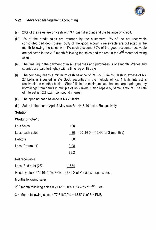
Advanced Management Accounting 5.22
(ii) 20% of the sales are on cash with 3% cash discount and the balance on credit.
(iii) 1% of the credit sales are returned by the customers. 2% of the net receivable constituted bad debt losses. 50% of the good accounts receivable are collected in the month following the sales with 1% cash discount, 30% of the good accounts receivable are collected in the 2nd month following the sales and the rest in the 3rd month following sales.
(iv) The time lag in the payment of misc. expenses and purchases is one month. Wages and salaries are paid fortnightly with a time lag of 15 days.
(i) The company keeps a minimum cash balance of Rs. 25.00 lakhs. Cash in excess of Rs. 27 lakhs is invested in 9% Govt. securities in the multiple of Rs. 1 lakh. Interest is receivable on monthly basis . Shortfalls in the minimum cash balance are made good by borrowings from banks in multiple of Rs.2 lakhs & also repaid by same amount. The rate of interest is 12% p.a. ( compound interest)
(ii) The opening cash balance is Rs.26 lacks.
(iii) Sales in the month April & May was Rs. 44 & 40 lacks. Respectively.
Solution
Working note-1:
Lets Sales 100
Less: cash sales 20 20×97% = 19.4% of S (monthly)
Debtors 80
Less: Return 1% 0.08
79.2
Net receivable
Less: Bad debt (2%) 1.584
Good Debtors 77.616×50%×99% = 38.42% of Previous month sales.
Months following sales
2nd month following sales = 77.616´30% = 23.28% of 2nd PMS
3rd Month following sales = 77.616´20% = 15.52% of 3rd PMS

Budget & Budgetary Control 5.23
Cash Budget
July Aug. Sept. Oct. Nov. Dec.
Opening balance 26 26.96 27.10 27.87 27.43 27.27 Collection from sales: Cash sales 19.4% of B/s 7.76 7.76 9.7 9.7 11.64 12.61 Collection: 38.42% of Pms 13.06 15.37 15.37 19.21 19.21 23.05
23.28% of 2nd Pms 9.312 7.92 9.31 9.31 11.64 11.64
15.52% of 3rd PMs 6.83 6.21 5.28 6.21 6.21 7.76 int-Business — — 2 — — 2 Govt. Bond — — 0.11 0.13 0.14 0.16 Sales — 20 — — — — (a) Total 62.96 84.22 68.87 72.43 76.27 84.49 Payments-Pm (1 m lag) 24 16 7 20 20 25 - Mis exps (1 m lag) 5 6 6 6 7 7 -wages & salary (1/2 m lag) 7 7 9 9 10 113 ½ of PM 6 7 7 9 9 10 (b) Total 42 36 39 44 46 53 (c) Gross balance 20.96 44.22 29.87 28.43 30.27 31.49 (d) Borrowing 6 — — — — — (e) Refund of borrowing with interest — 6.12 — — — — (f) Inv. in govt. bond — 15 2 1 3 4 (g) Net cash balance 26.96 27.10 27.87 27.43 27.27 27.49
Note-2: For July minimum balance 25,00,000 Less: Present balance 20,96,000 4,04,000 � Borrowing should be arranged in the multiple of 2 lakhs = 6 lakhs. The borrowing should be arranged should be arranged from the day 1 of the month. For Assessment year 48.22

Advanced Management Accounting 5.24
Less: Borrowing 6
Int. 6 (1.1)2 (approx) 0.12 @ 1% p.m. –6,000
Int. [A (1+i) n-A] _____ 42.10 Less: Minimum for investment 27 Fund for investment 15.10 �investment in Govt. bonds 15,00,000
The loans/borrowing at the 1st salary of the month of short falls & will be repaid in the last date of the subsequent month when the closing balance of cash is among hence a minimum interest period is 2 months. Illustration
The 1st January cash balance of the Jay Company is Rs. 5,000 . Sales for the first four months of the year are expected to be as follows: January, Rs. 65,000; February, Rs. 54,000; March, Rs. 66,000; and April, Rs. 63,000. On January1, uncollected amounts for November and December of the previous year, are Rs. 13,500 and Rs. 39,150, respectively. Collections from customers follow this pattern; 55% in the month of sale, 30% in the month following the sale, 13% in the second month following the sale, and 2% un-collectible. Materials purchases for December were Rs. 10,000. Forecast purchases for the coming year are January, Rs. 12,500; February, Rs. 16,500; March, Rs. 13,000; and April, Rs. 14,000. Purchases are usually paid by the 10th of the month following the month of purchase. Other cash expenditures of Rs. 41,000 are forecast for each month. Calculate : (i) Expected cash collections during February (ii) Expected cash balance, February1 (iii) Expected cash balance, February 28. Solution Working note-1 Sales 100
Less: Cash sales 55 1st month Debtors 45

Budget & Budgetary Control 5.25
Collection 30% in next month 30 2nd month following sales 15
Less: in 2 months 13 3rd month following sales Bad debt 2
Cash budget Jan Feb March April Opening cash balance 5,000 27,550 — — Collection: Cash sales @ 55% 35,750 29,700 36,300 34,650 Collection pm @ 30% of sales 26,100 19,500 16,200 19,800
Coll. of 2nd Pm @ 13% of sales 11,700 11,310 8,450 7,020 Total (a) 78,550 88,060 Payments: -purchase of material 1 months 10,000 12,500 16,500 13,000 -Mix expense 41,000 41,000 Total B 51,000 53,500 Net cash Balance (A-B) 27,550 34,560 Illustration The following is the Sales Budget of a company engaged in manufacturing and marketing certain consumer products (in 3 lines), their markets being Eastern and Western Zones.
Rs. in lakhs
Product Eastern Western Total Units Rs. Units Rs. Units Rs.
A 30,000 15.00 16,000 8.00 46,000 23.00 B 10,000 6.00 15,000 9.00 25,000 15.00 C 4,000 3.20 6,000 4.80 10,000 8.00 24.20 21.80 46.00

Advanced Management Accounting 5.26
NO changes are expected in the inventory levels. The following are the unit standard cost details for the 3 products :–
A B C Rs. Rs. Rs.
Direct Materials Material X @ Rs. 6 per kg. 12 24 18 Material Y @ Rs. 4 per kg 8 — 4 Direct Labour: Rs. 4 per hour 12 16 20 Factory Overheads: Variable @ Re. 1.00 per Std. Hr. 3 4 5 Fixed @ Rs. 2.00 per Std. Hr. 6 8 10
Variable Overheads comprise Indirect Material, Indirect Labour and Indirect Expenses in the ratio of 50 : 25 : 25. Fixed Factory overheads stated above are based on the following Product Mix:– Product A 20,000 units Product B 15,000 units Product C 10,000 units The mix of fixed factory overheads consists of Indirect material, Indirect Labour and Indirect Expenses in the ratio of 30 : 30 : 40. Price of Material X is expected to increase by Re. 0.20 per kg. in the budget period. There will be 2% inefficiency (i.e. 2% wastage allowance) in case of Direct Materials. A 3% increase in productivity of direct labour is expected. No other variances in direct costs are expected. Therese variances and any other variances in indirect items have to be built into the Budgets. The selling and Distribution cost budget for the two zones are as follows :–
Eastern Western
Zonal Manager’s Control Commission 10% on 10% Std. gross Std. gross Profit Profit Rs. Rs. Travelling 40,000 35,000

Budget & Budgetary Control 5.27
Advertising 15,000 12,000 Office Fixed expenses: Salaries 20,000 20,000 Perquisites 2,000 2,000 Depreciation 5,000 4,000 Insurance 1,000 1,000
The head office selling and distribution expenses are: Advertising and Sales Promotion Rs. 70,000; Salaries Rs. 42,000; Stationary Postage etc. Rs. 5,000; Depreciation Rs. 5,000; insurance Rs. 1,000. Head Office Administrative expenses are Rs. 2,00,000 and this should be met out of gross profit. The average rate of Tax is 40%. You are required to prepare the Budgeted Income Statement for the Company. Solution Budgeted Income Statement for the period … Product Rs. Rs. Sales: A 23,00,000 B 15,00,000 C 8,00,000 (A) 46,00,000 Less: Cost of Goods Sold : Direct Materials : X 14,03,928 (see note 1) 4,16,160 18,20,088 Direct Labour : (see note 2) 11,17,440 Factory Overhead : Variable : Indirect Material 1,44,400 (see note 3) Indirect Labour 72,000 Indirect Expenses 72,000 2,88,000 Fixed : Indirect Material (see note 4) 1,02,000 Indirect Labour 1,02,000 Indirect Expenses 1,36,000 3,40,000

Advanced Management Accounting 5.28
Total Factory Cost of Sales (B) 35,65,528 Gross Profit (A–B) (C) 10,34,472 Less : Head Office Expenses : Administration 2,00,000 Selling & Distribution 1,23,000 3,23,000 Selling, Distribution and other Fixed Expense of the Two Zones : Commission (Note 5) 84,400 Travelling Expenses 75,000 Advertising 27,000 Office Expenses 18,000 Salaries & Perks 44,000 Depreciation 9,000 Insurance 2,000 2,59,400 Total Adm. & Selling Expenses (D) 5,82,400 Net Profit (C–D) (E) 4,50,072 Less Tax @ 40% 1,80,829 Profit After Tax 2,71,243 Working Notes : (1) Calculation of Direct Material Cost : Product Material X Material Y Kgs. Kgs. A 46,000 × 2 92,000 46,000 × 2 92,000 B 25,000 × 4 1,00,000 — C 10,000 × 3 30,000 10,000 × 1 10,000 Total material required as per _______ _______ standard 2,22,000 1,02,000 Add 2% wastage allowance (assumed to be based on output) 4,440 2,040 Total Material Requirement 2,26,440 1,04,040 Material Cost Price per kg.Rs. 6.20 Rs. 4 Total material Cost Rs. 14,03,928 4,16,160

Budget & Budgetary Control 5.29
(2) Calculation of Direct Labour Cost : Product Hrs. A 46,000 × 3 hrs. 1,38,000 B 25,000 × 4 hrs. 1,00,000 C 10,000 × 5 hrs. 50,000 2,88,000 Less :Saving of 3% due to efficiency 8,640 Hours to be paid for 2,79,360 Total Direct Labour Cost (2,79,360 @ Rs. 4/- per hour) Rs.11,17,440 (3) Calculation of Variable Factory Overheads : Product Rs. A 46,000 units @ Rs. 3 per unit 1,38,000 B 25,000 units @ Rs. 4 per unit 1,00,000 C 10,000 units @ Rs. 5 per unit 50,000 2,88,000 (Indirect Material Cost Rs. 1,44,000 : Indirect Labour Cost Rs. 72,000; and Indirect Expenses Rs. 72,000— in the ratio of 50 : 25 : 25 respectively) (4) Calculation of Fixed Factory Overheads: Product A 20,000 units @ Rs. 6 per unit 1,20,000 B 15,000 units @ Rs. 8 per unit- 1,20,000 C 10,000 units @ Rs. 10 per unit 1,00,000 3,40,000 (Indirect Material Cost Rs. 1,02,000; Indirect Labour Cost Rs. 1,02,000; and Indirect Expenses Rs. 1,36,000— in the ratio of 30 : 30 : 40 respectively)

Advanced Management Accounting 5.30
(5) Calculation of Commission of the 2 Zones: Standard Gross Profit per unit: Eastern Western Rs. Rs. (Selling price – Std. cost price) A 50 – 41 = 9 50 – 41 9 B 60 – 52 = 8 60 – 51 8 C 80 – 57 = 23 80 – 57 23 Std. Gross Profit for Zones: A 30,000 × 9 = 2,70,000 16,000 × 9 =1,44,000 B 10,000 × 8 = 80,000 15,000 × 8 =1,20,000 C 4,000 × 23 = 92,000 6,000 × 23 = 1,38,000 Total Gross Profit 4,42,000 4,02,000 10% of the above 44,200 40,200 Total Rs. 84,400 Illustration S. G. Ltd. manufactures two products A and B. The summarised Balance Sheet of the company as at 30th September, 1988 is as under :– Rs. Rs. Share Capital 12,00,000 Retained Income 96,000 12,96,000 Represented by:– Fixed Assets 1?,00,000 Provision for Depreciation 3,00,000 9,00,000 Inventories:– Raw materials 1,14,000 Finished goods 2,40,000 3,54,000 Debtors 90,000 Bank/cash 60,000 14,04,000 Less: Creditors 48,000 Provision for taxation 60,000 1,08,000 12,96,000

Budget & Budgetary Control 5.31
The following information has been furnished to you for the preparation of the budget for the year ending 30th September, 1989 :– (i) Sales forecast :– Product A 24,000 units at Rs. 30 per unit. Product B 15,000 units at Rs. 40 per unit. (ii) Raw materials :–
Products A B Material X @ Rs. 3 per kg. 2 kgs. 4 kgs. Material Y @ Re. 1 per kg. 1 kg. 2 kgs. (iii) Direct Labour :– Dep. P : 2 Hrs. @ Re. 1 per hour for A. 1 Hr. @ Rs. 2 per hour for B. Dep. Q: 1 Hr. @ Rs. 3 per hour for A 1 Hr. @ Rs. 3 per hour for B. (iv) Overheads :– Dept. P Dept. Q Rs. Rs. Fixed overheads per annum :– Depreciation 48,000 12,000 Others 96,000 30,000 Variable overheads per hour 0.50 1.50 (v) Inventories :– (a) Raw materials : Opening stock X 36,000 kgs. Y 6,000 kgs. Closing stock X 48,000 kgs. Y 12,000 kgs.

Advanced Management Accounting 5.32
(b) Finished goods : Opening stock A 600 units B 6,000 units Closing stock A 6,600 units B 3,000 units (vi) Selling, Distribution and Administration expenses are estimated at Rs. 1,80,900 per
annum. (vii) The cost of raw material purchases, direct wages, factory overheads, selling, distribution
and administration overheads of the year will be met in full in cash during the year. The estimated position of debtors and creditors as on 30th September, 1989 is Rs. 1,50,000 and Rs. 48,000 respectively. Income tax provision standing at the beginning of the year will be paid during the year. Rate of income tax is 50%. An equipment purchased at Rs. 1,20,000 will be paid during the year.
You are required to prepare for the year ending 30th September, 1989:– a) Cost of goods sold budget b) Cash budget
c) Projected Balance Sheet as at 30th September, 1989 in the same format as given in the question.
The detailed working for each of the above should be shown. Solution Working Notes: 1. Production Budget (Units) A B Total Sales 24,000 15,000 Add : Closing Stock 6,600 3,000 Total 30,600 18,000 Less : Opening Stock 600 6,000 Production 30,000 12,000
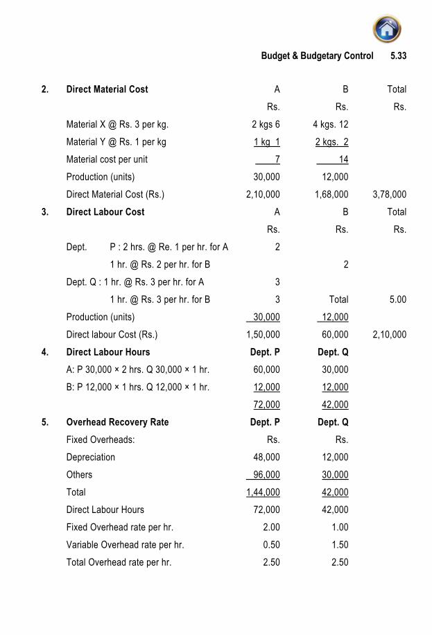
Budget & Budgetary Control 5.33
2. Direct Material Cost A B Total Rs. Rs. Rs. Material X @ Rs. 3 per kg. 2 kgs 6 4 kgs. 12 Material Y @ Rs. 1 per kg 1 kg 1 2 kgs. 2 Material cost per unit 7 14 Production (units) 30,000 12,000 Direct Material Cost (Rs.) 2,10,000 1,68,000 3,78,000 3. Direct Labour Cost A B Total Rs. Rs. Rs. Dept. P : 2 hrs. @ Re. 1 per hr. for A 2 1 hr. @ Rs. 2 per hr. for B 2 Dept. Q : 1 hr. @ Rs. 3 per hr. for A 3 1 hr. @ Rs. 3 per hr. for B 3 Total 5.00 Production (units) 30,000 12,000 Direct labour Cost (Rs.) 1,50,000 60,000 2,10,000 4. Direct Labour Hours Dept. P Dept. Q A: P 30,000 × 2 hrs. Q 30,000 × 1 hr. 60,000 30,000 B: P 12,000 × 1 hrs. Q 12,000 × 1 hr. 12,000 12,000 72,000 42,000 5. Overhead Recovery Rate Dept. P Dept. Q Fixed Overheads: Rs. Rs. Depreciation 48,000 12,000 Others 96,000 30,000 Total 1,44,000 42,000 Direct Labour Hours 72,000 42,000 Fixed Overhead rate per hr. 2.00 1.00 Variable Overhead rate per hr. 0.50 1.50 Total Overhead rate per hr. 2.50 2.50

Advanced Management Accounting 5.34
6. Overhead Expenses Dept P Dept Q Total Rs. Rs. Rs. Fixed Other than Depreciation 96,000 30,000 Variable 72,000 × Re. 0.50 36,000 42,000 × Rs. 1.50 _ 63,000 Total 1,32,000 93,000 225,000 Depreciation 48,000 12,000 60,000 Total Overheads 1,80,000 1,05,000 285,000 7. Cost Sheet Products A B Rs. Rs. Direct material per unit 7.00 14.00 Direct wages per unit 5.00 5.00 Overhead P per unit 5.00 2.50 Q per unit 2.50 2.50 _ Total cost per unit 19.50 24.00 Production 30,000 12,000 Total cost 5,85,000 2,88,000 8,73,000 8. Sales Rs. A 24,000 × Rs. 30 7,20,000 B 15,000 × Rs. 40 6,00,000 Total 13,20,000 9. Debtors Rs. Opening Balance 90,000 Sales 13,20,000 Total 14,10,000 Closing Balance 1,50,000 Cash Receipts 12,60,000

Budget & Budgetary Control 5.35
10. Raw Material Products Material X (kgs.) Y (kgs.) Total X Y Rs. Kg. Kg. A 30,000 units 2 1 60,000 30,000 B 12,000 units 4 2 48,000 24,000 1,08,000 54,000 Closing Stock 48,000 12,000 Total 1,56,000 66,000 Opening Stock 36,000 6,000 Material to be purchased 1,20,000 60,000 Purchase price per ??? Rs. 3 Rs. 1 Purchase value (Rs.) 3,60,000 60,000 4,20,000 11. Creditors Rs. Opening Balance 48,000 Purchases 4,20,000 Total 4,68,000 Closing Balance 48,000 Paid 4,20,000 12. Inventories as on 30-9,1989 Raw material :X 48,000 × Rs. 3 = 1,44,000 Y 12,000 × Re. 1 = 12,000 1,56,000 Finished Goods : A 6,600 × Rs. 19.50 = 1,28,700 B 3,000 × Rs. 24.00 = 72,000 2,00,700 (a) Cost of Goods Sold Budget Rs. Direct Materials (Note 2) 3,78,000 Direct Wages (Note 3) 2,10,000 Overheads (Note 6) 2,85,000 Total 8,73,000 Add : Op. Stock (Balance Sheet) 2,40,000

Advanced Management Accounting 5.36
Total 11,13,000 Less: Closing Stock (Note 12) 2,00,700 Cost of Goods sold 9,12,300 (b) Cash Budget Rs. Opening Balance (Balance Sheet)60,000 Receipts (Note 9) 12,60,000 Total receipts (A) 13,20,000 Payments : Creditors (Note 11) 4,20,000 Direct Wages (Note 3) 2,10,000 Overheads (Note 6) 2,25,000 Selling, Distribution and Administration Expenses, 1,80,900 Income Tax 60,000 Capital Expenditure 1,20,000 Total Payments (B) 12,15,900 Closing Balance (A – B) 1,04,100
(c) Projected Balance Sheet as at 30th September, 1989: Rs. Rs. Share Capital 12,00,000 Retained Income* 2,09,400 14,09,4000 Represented by :– Fixed Assets 12,00,000 Additions 1,20,000 13,20,000 Provision for Depreciation 3,60,000 9,60,000 Inventories :– Raw Materials 1,56,000 Finished Goods 2,00,700 3,56,700 Debtors 1,50,000
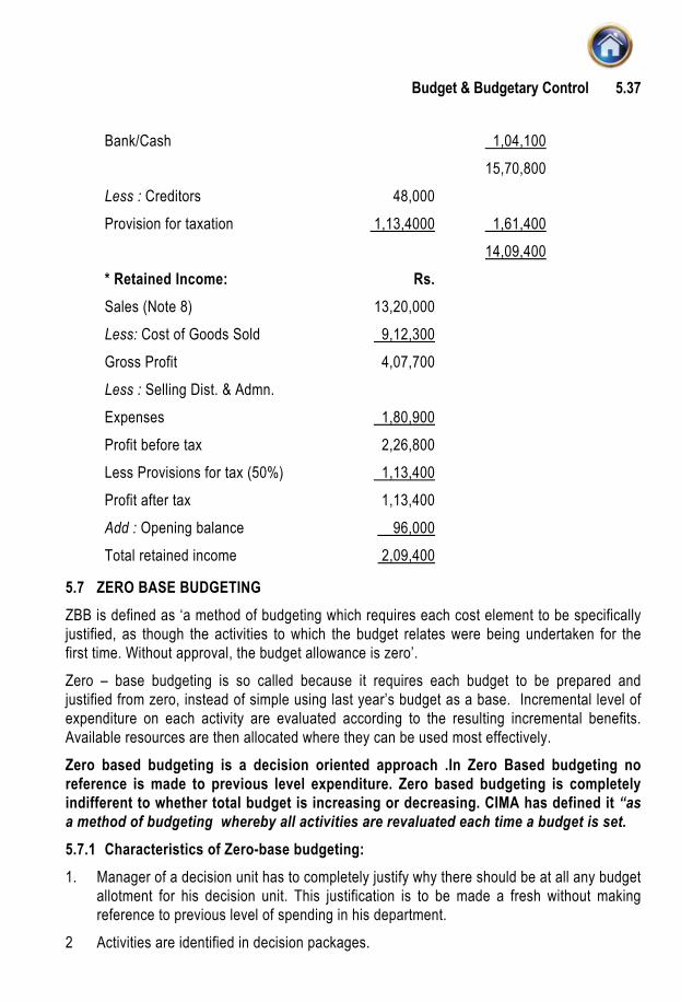
Budget & Budgetary Control 5.37
Bank/Cash 1,04,100 15,70,800 Less : Creditors 48,000 Provision for taxation 1,13,4000 1,61,400 14,09,400 * Retained Income: Rs. Sales (Note 8) 13,20,000 Less: Cost of Goods Sold 9,12,300 Gross Profit 4,07,700 Less : Selling Dist. & Admn. Expenses 1,80,900 Profit before tax 2,26,800 Less Provisions for tax (50%) 1,13,400 Profit after tax 1,13,400 Add : Opening balance 96,000 Total retained income 2,09,400
5.7 ZERO BASE BUDGETING ZBB is defined as ‘a method of budgeting which requires each cost element to be specifically justified, as though the activities to which the budget relates were being undertaken for the first time. Without approval, the budget allowance is zero’. Zero – base budgeting is so called because it requires each budget to be prepared and justified from zero, instead of simple using last year’s budget as a base. Incremental level of expenditure on each activity are evaluated according to the resulting incremental benefits. Available resources are then allocated where they can be used most effectively. Zero based budgeting is a decision oriented approach .In Zero Based budgeting no reference is made to previous level expenditure. Zero based budgeting is completely indifferent to whether total budget is increasing or decreasing. CIMA has defined it “as a method of budgeting whereby all activities are revaluated each time a budget is set. 5.7.1 Characteristics of Zero-base budgeting: 1. Manager of a decision unit has to completely justify why there should be at all any budget
allotment for his decision unit. This justification is to be made a fresh without making reference to previous level of spending in his department.
2 Activities are identified in decision packages.

Advanced Management Accounting 5.38
3 Decision packages are ranked in order of priority. 4 Packages are evaluated by systematic analysis. 5 under this approach there exist a frank relationship between superior and subordinates.
Management agrees to fund for a specified service and manager decision of the decision unit clearly accepts to deliver the service.
6 Decision packages are linked with corporate objectives, which are clearly laid down. 7 Available resources are directed towards alternatives in order of priority to ensure
optimum results. 5.7.2 Traditional Budgeting vs Zero- based budgeting.Following are the points of difference between traditional budgeting and zero based budgeting: 1. Traditional budgeting is accounting oriented. Main stress happens to be on previous level
of expenditure. Zero-based budgeting makes a decision oriented approach. It is very rational in nature and requires all programmes, old and new, to compete for scarce resources.
2. In traditional budgeting, first reference is made to past level of spending and then demand for inflation and new programmes. In zero based budgeting a decision unit is broken into understandable decision packages, which are ranked according to importance to enable to top management to focus attention to only on decision packages, which enjoy priority to others.
3. In tradition budgeting, some managers deliberately inflate their budget request so that after the cuts they still get what they want. In zero-base budgeting, a rationale analysis of budget proposals is attempted. The managers, who unnecessarily try to inflate the budget request, are likely to be caught and exposed. Management accords its approval only to a carefully devised result-oriented package.
4. Traditional budgeting is not as clear and as responsive as zero base budgeting is. 5. In traditional budgeting. Its for top management to decide why a particular amount should
be spent on a particular decision unit. In Zero-base budgeting, this responsibility is shifted from top management to the manager of decision unit.
6. Traditional budgeting makes a routine approach. Zero-base budgeting makes a very straightforward approach and immediately spotlights the decision packages enjoying priority over others.
5.7.3 Process of Zero-base Budgeting: The process of zero-base budgeting involves the following steps: 1. Determination of a set of objectives is one of pre-requisites and essential step in the
direction of ZBB technique. 2. Deciding about the extent to which the technique of ZBB is to be applied whether in all
areas of organizations’ activities or only in a few selected areas on trial basis.
Budget & Budgetary Control 5.39
3. Identify those areas where decisions are required to be taken. 4. Developing decision packages and ranking them in order of performance. 5. Preparation of budget that is translating decision packages into practicable units/items
and allocating financial/resources. In real terms the Zero base budgeting is simply an extension of the cost, benefit, analysis method to the area of corporate planning and budgeting. It, however, provides a number of advantages to the organizational efficiency and effectiveness. 5.7.4 Advantages of Zero-base budgeting: The advantages of zero-base budgeting are as follows: 1. It provides a systematic approach for the evaluation of different activities and rank them
in order of preference for the allocation of scarce resources. 2. It ensures that the various functions undertaken by the organization are critical for the
achievement of its objectives and are being performed in the best possible way. 3. It provides an opportunity to the management to allocate resources for various activities
only after having a thorough cost-benefit-analysis. The chances of arbitrary cuts and enhancement are thus avoided.
4. The areas of wasteful expenditure can be easily identified and eliminated. 5. Departmental budgets are closely linked with corporation objectives. 6. The technique can also be used for the introduction and implementation of the system of
‘management by objective.’ Thus, it cannot only be used for fulfillment of the objectives of traditional budgeting but it can also be used for a variety of other purposes.
5.7.5 Zero base budgeting s superior to traditional budgeting • Zero base budgeting s superior to traditional budgeting in the following manner : • It provides a systematic approach for evaluation of different activities. • It ensure that the function undertaken are critical for the achievement of the objectives. • It provides an opportunity for management to allocate resources to various activities after
a through – cost benefit analysis. • It helps in the identification of wasteful expenditure and then their elimination. If
facilitates the close linkage of departmental budgets with corporate objectives • It helps in the introduction of a system of Management by Objectives. 5.7.6 Disadvantage of ZBB: 1. The work involves in the creation of decision-making and their subsequent ranking has to
be made on the basis of new data. This process is very tedious to management. 2. The activity selected for the purpose of ZBB are on the basis of the traditional functional
departments. So the consideration scheme may not be implemented properly.

Advanced Management Accounting 5.40
5.8 PERFORMANCE BUDGETING (PB) Performance Budgeting provide a meaningful relationship between estimated inputs and expected outputs as an integral part of the budgeting system. ‘A performance budget is one which presents the purposes and objectives for which funds are required, the costs of the programmes proposed for achieving those objectives, and quantities data measuring the accomplishments and work performed under each programme. Thus PB is a technique of presenting budgets for costs and revenues in terms of functions. Programmes and activities are correlating the physical and financial aspect of the individual items comprising the budget. 5.8.1 Traditional budgeting vs. Performance budgeting 1. The traditional budgeting (TB) gives more emphasis on the financial aspect than the
physical aspects or performance. PB aims at establishing a relationship between the inputs and the outputs.
2. Traditional budgets are generally prepared with the main basis towards the objects or items of expenditure i.e. it highlights the items of expenditure, namely, salaries, stores and materials, rates rents and taxes and so on. In the PB latter the emphasis is more on the functions of the organisation, the programmes to discharge these function and the activities which will be involved in undertaking these programmes.
Steps in Performance Budgeting : According to the Administrative Reforms Commission (ARC) the following steps are the basic ones in PB : (a) establishing a meaningful functional programme and activity classification of government
operations ; (b) bring the system of accounting and financial management in accord with this
classification (c) evolving suitable norms, yardsticks, work units of performance and units costs, wherever
possible under each programme and activity for their reporting and evaluation. The Report of the ARC use the following terms in an integrated sequence : Function Programme Activity Project The team ‘function’ is used in the sense of ‘objective’. For achieving objectives ‘programmes’ will have to be evolved. In respect of time horizon, it is essentially a replacement of traditional annual fiscal budgeting by a more output-oriented, but still an annual, exercise. For an enterprise that wants to adopt PB, it is thus imperative that : (a) the objectives of the enterprise are spelt out in concrete terms. (b) the objectives are then translated into specific functions, programmes, activities and
tasks for different levels of management within the realities of fiscal; constraints ;

Budget & Budgetary Control 5.41
(c) realistic and acceptable norms, yardsticks or standards and performance indicators should be evolved and expressed in quantifiable physical units.
(d) a style of management based upon decentralised responsibility structure should be adopted, and
(e) an accounting and reporting system should be developed to facilities monitoring, analysis and review of actual performance in relation to budgets.
Performance Reporting at various levels of management: Report: A major part of the management account’s job consists of preparing reports to provide information for purposes of control and planning: The important consideration in drawing up of reports and determining their scope are the following: Significance : Are the facts in the reports reliable? Does it either called for action or
demonstrate the effect of action? It is material enough. Timeliness : How late can the information be and still be of use? What is the earliest
moment at which it could be used if it were available? How frequently is it required.
Accuracy : How small should be an inaccuracy which does not alter the significance of he information?
Appropriateness : Is the recipient the right person to take any action that is needed? Is there any other information which is required to support the information to anyone else jointly interested?
Discrimination : Will anything be lost by omitting the item? Will any of the items gain from the omission ? Is the responsibility for suppressing the item acceptable?
Presentation : Is the report clear and unbiased? Is the form of it is suitable to the subject? Is the form of it suitable to the recipient?
The following are certain types of reports which are to be prepared and submitted to management regularly at predetermined time interval:- 1. Top management: (Including Board of Directors and financial managers) i) Balance Sheet ii) Profit & Loss Statement iii) Position of stocks iv) Disposition of funds or working capital; v) Capital expenditure & forward commitments together with progress of projects in hands; vi) Cash-flow statements; vii) Sales, production, and other appropriate statistics.

Advanced Management Accounting 5.42
2. Sales Management: 1. Actual sales compared with budgeted sales to measure performance by: a) Products, b) Territories c) Individual salesmen, and d) Customers. 2. Standard profit and loss by product: a) For fixing selling prices, and b) To Concentrate on sales of most profitable products. 3. Selling expenses in relation to budget and sales value analyzed by: a) Products, b) Territories c) Individual salesmen, and d) Customers. 4. Bad debts and accounts which are slow and difficult in collection. 5. Status reports on new or doubtful customers.
3. Production Management: i) To Buyer: Price variations on purchases analysed by commodities. ii) To Foreman:
a) Operational efficiency for individual operators duly summarized as departmental average;
b) Labour utilization report and causes of lost time and controllable time; c) Indirect shop expenses against the standard allowed; and d) Scrap report.
iii) To Works Managers: a) Departmental operating statement; b) General works operating statements (Expenses relating to all works expenses
not directly allocable or controllable by departments); c) Plant utilization report; d) Department Scrap report; and e) Material usage report.

Budget & Budgetary Control 5.43
4. Special Reports: Theses reports may be prepared at the request of general management or at the initiative of the management accountant. The necessity for them may, in some cases, arise on account of the need for more detailed information on matters of interest first revealed; by the routine, reports. These reports may range over a very wide area. Some of the matters in respect of which such reports may be required can be: i) Taxation legislation and its effect on profits. ii) Estimates of the earning capacity of a new project. iii) Break-even analysis iv) Replacement of capital equipment. v) Special pricing analysis vi) Make or buy certain components vii) Statement of surplus available for payment of bonus under the labour appellate tribunal
formula.
5.9 BUDGET RATIO These ratios provide information about the performance level, i.e., the extent of deviation of actual performance from the budgeted performance and whether the actual performance is favourable or unfavorable. If the ratio is 100% or more, the performance is considered as favourable and if ratios is less than 100% the performance is considered as unfavourable. The following ratios are usually used by the management to measure development from budget. Capacity usage ratio: This relationship between the budgeted number of working hours and the maximum possible number of working hours in a budget period. Standard capacity employed ratio: this ratio indicates the extent to which facilities were actually utilized during the budget period. Level of activity ratio: This may be defined as the number of standard hours equivalent to work produced expressed as a percentage of the budget of standard hours. Efficiency ratio: this ratio may be defined as standard hours equivalent of work produced expressed as a percentage of the actual hours spent in producing the work. Calendar ratio: This ratio may be defined as the relationship between the number of working days in a period and the number of working das in the relative budget period. Budget Ratios : 1. Efficiency Ratio = (Standard hours ÷ Actual hours) × 100
2. Activity Ratio = (Standard hours ÷ Budgeted hours) × 100

Advanced Management Accounting 5.44
3. Calendar Ratio = (Available working days ÷ budgeted working days) × 100
4. Standard Capacity Usage Ratio = (Budgeted hours ÷ Max. possible hours in the budgeted period) × 100
5. Actual Capacity Usage Ratio = (Actual hours worked ÷ Maximum possible working hours in a period) × 100
6. Actual Usage of Budgeted Capacity Ratio = (Actual working hours ÷ Budgeted hours) × 100
Illustration Following data is available for T.T.D and Co: Standard working hours 8 hours per day of 5 days per week Maximum capacity 50 employees Actual working 40 employees Actual hours expected to be worked per four week 6,400 hours Std. hours expected to be earned per four weeks 8,000 hours Actual hours worked in the four week period 6,000 hours Standard hours earned in the four week period 7,000 hours. The related period is of 4 weeks. In this period there was a one special day holiday due to national event. Calculate the following ratios : (1) Efficiency Ratio, (2) Activity Ratio, (3) Calendar Ratio, (4) Standard Capacity Usage Ratio, (5) Actual Capacity Usage Ratio. (6) Actual Usage of Budgeted Capacity Ratio. Solution Maximum capacity in a budget period = 50 employees × 8 hrs.×5 days×4 weeks = 8,000 hrs. Budgeted hours 40 employees ×8 hrs.×5 days×4 weeks = 6,400 hrs. Actual hrs. = 6,000 hrs. (from the sum) Standard hrs. for actual output = 7,000 hrs. Budget no. of days = 20 days = 20 days (4 weeks ´5 days) Actual no. of days = 20 – 1 = 19 days

Budget & Budgetary Control 5.45
1. Efficiency ratio = Standard hrsActual hrs.
×100 = {(7,000÷6,000)×100} = 116.67%
2. Activity ratio = {(7,000÷6,400)×100} = 109.375%
3. Calendar Ratio = (Available working days ÷ budgeted working days) × 100
= {(19÷20)×100} = 95% 4. Standard Capacity Usage Ratio =
(Budgeted hours ÷ Max. possible hours in the budgeted period) × 100
= {(6,400÷8,000)×100} = 80% 5. Actual Capacity Usage Ratio =
(Actual hours worked ÷ Maximum possible working hours in a period) × 100
= {(6,000÷8,000)×100} = 75% 6. Actual Usage of Budgeted Capacity Ratio =
(Actual working hours ÷ Budgeted hours) × 100
= {(6,000÷6,400)×100} = 93.75%
5.10 BUDGET VARIANCE It is computed on the basis of fixed budgeting system where budget variance = budgeted cost – actual cost here. The items are classified first in respective responsibility category & then the differences are computed individually & totally. Illustration Nicefit Manufactures ready made garments by a simple process of cutting the clothes in various shapes and then sewing the corresponding pieces together to form the finished product. The sewing Department and the cutting department report to the production manager who along with Engineering Manager reports to the Director-Manufacturing. The Sales Manager, Publicity Manager and the Credit Manger report to the Director-Marketing, who along with Direct-Manufacturing reports to the Managing Director of the company. The Accounts Department reports the following for the last quarter of 1983: Budgeted Rs. Actual Rs. Bad debt Losses 5,000 3,000 Cloth used 31,000 36,000 Advertising 4,000 4,000 Audit fees 7,500 7,500

Advanced Management Accounting 5.46
Credit reports 1,200 1,050 Sales representative Travelling expenses 9,000 10,200 Sales commission 7,000 7,000 Cutting Labour 6,000 6,600 Thread 500 450 Sewing Labour 17,000 18,400 Credit Deptt. Salaries 8,000 8,000 Cutting utilities 800 700 Sewing utilities 900 950 Director Marketing salaries & Admn. Exp. 20,000 21,400 Production engineering expenses 13,000 12,200 Sales management office expenses 16,000 15,700 Production Manger office expenses 18,000 17,000 Direct Mfg. Salaries & Admn. Expenses 21,000 20,100 Using the above data, prepare responsibility Accounting reports for the director marketing, the Director-manufacturing and the production manager. Answer
Responsibility Accounting Reports For the production manager
Cutting Department Budgeted Rs. Actual Rs. Variance Rs. Cloth 31,000 36,000 5,000 (A) Cutting Labour 6,000 6,600 600 (A) Cutting utilises 800 700 100 (A) Total cutting Deptt. (A) 37,800 43,300 5,700 (A) Sewing Department: Thread 500 450 50 (F) Sewing Labour 17,000 18,400 1,400 (A) Sewing utilities 900 950 50(F) Total Sewing Dept. (B) 18,400 19,800 1,400 (A) Total (A + B) 56,200 63,100 6,900 (A)

Budget & Budgetary Control 5.47
For the director-Manufacturing Production Department * 56,200 63,100 6,900 (A) Production engineering expenses 13,000 12,200 800 (F) Production manager-office expenses 18,000 17,000 1,000 (F) Total 87,200 92,300 5,100 (A) (* As per responsibility accounting report for the production manager)
for the Direct-Marketing Sales representative: Travelling expenses 9,000 10,200 1,200 (A) Sales commission 7,000 7,000 -- Total (A) 16,000 17,200 1,200 (A) Sales Management: Office expenses 16,000 15,700 300 (F) Advertising 4,000 4,000 — Total (B) 20,000 19,700 300 (F) Credit Department: Salaries 8,000 8,000 Credit reports 1,200 1,050 150 (F) Bad debt Losses 5,000 3,000 2,000 (F) Total 14,200 12,050 2,150 (F) Total (A + B + C) 50,200 48,950 1,250 (F) Note: ‘F’ denotes favourable variance while ‘A’ denotes adverse variance. Illustration The following data relate to a company which had a profit approved for selling 5000 units per month at an average selling price of Rs. 10 per unit and budgeted variable cost of production was Rs. 4 per unit and fixed costs were budgeted at Rs. 20,000. Planned income being Rs. 10,000 per month. Because of shortage of raw—materials the plant could produce only 4000 units and the cost of production was increased by 0.50 per unit. Consequently Rs. 1.00 raised the selling price per unit. To modify production processes in order to meet materials shortage, the Company incurred an expenditure of Rs. 1,000 in Research and Development. Set out a Performance budget and a summary report there.

Advanced Management Accounting 5.48
Solution Performance Budget
Original Revised Actual Variance
Plan Rs. Budgeted Rs. Result Rs. Rs.
Revenue (5,000×10) 50,000
(4,000×10) 40,000
(4,000×11) 44,000 4,000 (F)
Variable (5,000×4) 20,000
Costs (4,000×4) 16,000
(4,000×4.5) 18,000 2,000 (A)
Contribution (5,000×4) 30,000
(4,000×6) 24,000
(4,000×6.5) 26,000 2,000 (F)
Fixed costs 20,000 20,000 21,000 1,000 (A)
Net Profit 10,000 4,000 5,000 1,000 (F)
Summary Report on Profit Plan
Planned Income (from Project plan) Rs. 10,000
Activity variance (lost contribution margin due
to shortage of materials) (6,000)
Selling price variance (increased
Selling price of Re. 1/- per unit) 4,000
Variance cost variance (increased production
Costs at 0.50 per unit) (2,000)
Fixed cost variance (new research programme to
Develop raw materials and processes) (1,000)
Actual income (from income statement) 5,000

Budget & Budgetary Control 5.49
SUMMARY • Three types of planning :
Budgetory Strategic Operational
• Budget Ratios: Efficiency Ratio = (Standard hours ÷Actual hours) × 100 Activity Ratio = (Standard hours ÷ Budgeted hours) × 100 Calendar Ratio = (Available working days ÷ budgeted working days) × 100 Standard Capacity Usage Ratio = (Budgeted hours ÷ Max. possible hours in the
budgeted period) × 100 Actual Capacity Usage Ratio = (Actual hours worked ÷Maximum possible
working hours in a period) × 100 Actual Usage of Budgeted Capacity Ratio = (Actual working hours ÷ Budgeted
hours) × 100 • Key requirements in the design of a budgetary planning and control process
Co-ordination Participative Budgeting Informtaion Identification of the principal budget factor How to identify the principal budget factor
1. In single product 2. In multi product
• Zero Based budgeting is defined as a method of budgeting whereby all activities are revaluated each time a budget is set.
SELF-EXAMINATION QUESTIONS 1. Difference between strategic, budgetary and operational planning. 2. What do you understand by ‘principal budget factor’. How is it identified. a. in case of single product organisation. b. in case of multi product organisation.

Advanced Management Accounting 5.50
3. What is zero base budgeting. What are its advantages and disadvantages. 4. What do you mean by performance budgeting. How is it different from traditional
budgeting. Discuss. 5. What are budget ratios. List six such ratios which you are aware of.

6 Standard Costing
LEARNING OBJECTIVES : After studying this unit you will be able to :
• Understand terms as standard Cost, standard Costing, standard Hour
• Understand how a standard costing system operates
• Calculate material, labour, overhead, sales value and sales margin variances
• Explain the terms operational and planning variances
• Explain the difference between actual profit and profit as per standard relating to the operating period
6.1 INTRODUCTION
You were introduced to Standard Costing in the earlier stages of your studies in which you understood the following;
• The evolution of Standard Costing
• The meaning of a Cost Sheet and its use for computing variances.
• The process of setting standards
• Computation of basic variances like Material Usage and Price, Labour Rate and
• Efficiency, Production Volume and Overhead Expenses.
• The reporting pattern of these variances
• Reconciliation of variances so as to arrive at the actual costing profit.
• Advantages and disadvantages of Standard Costing.
• The Accounting procedure for Standard Cost.

Advanced Management Accounting 6.2
In this chapter we shall extend our understanding of this important topic by studying elaborately the computation of various variances and the behavioral impact they can have on concerned personals.
6.2 DEFINITIONS
Cost variance is the difference between standard cost and the actual cost incurred. .
Variance analysis is the analysis of the cost variances into its component parts with appropriate justification of such variances, so that we can approach for corrective measures. 6.2.1 Classification of Variances Variances can be established under material, labour & overheads. There are three distinct groups of variances that arise in standard costing which are
1) Variances of Efficiency
Variances due to the effective or ineffective use of materials quantities, labour hours, once actual quantities are compared with the predetermined standards.
2) Variances of Price Rates
Variances arising due to change in unit material prices, standard labour hour rates and standard allowances for indirect costs.
3) Variances Due to Volume Variance due to the effect of difference between actual activity and the level of activity
assumed when the standard was set. 6.2.2 Why Standard Costing
Standard Costing main purpose is to
• Investigate the reasons
• Identify the problems
• Take corrective action.
Variances are broadly of two types, controllable and uncontrollable. Controllable variances are those which can be controlled by the departmental heads whereas uncontrollable variances are those which are beyond control.
For example, price variance is normally regarded as uncontrollable if the price increase is due to market fluctuations. It becomes controllable if the production controller has failed to place orders in time and urgent purchase was made at extra cost. In the former case, no responsibility is attached to any one whereas the departmental head has responsibility for the loss in the latter case. Since all price variances are uncontrollable and are of significant nature and are persistent, the standard may need revision.

Standard Costing 6.3
The possible reasons for each type of variances and the suggested course of action are given below. This list is only illustrative and not exhaustive.
Type of Variance Reasons of Variance Suggestive Course of ActionMATERIAL Material Price • Change in Basic Price
• Fail to purchase the
anticipated standard quantities at appropriate price
• Departmental head should take necessary action to purchase at right point of time
• Cash discount or interest rate for payment of purchase should be consider at the time of such payment
• Price check on the purchase of standard quality materials
Material Usage • Use of sub-standard material
• Ineffective use of materials
• Pilferage • Non standardised mix
• Regular Inspection of quality of materials
• Proper training of operators
• Ensure best utilisation of resources
LABOUR Labour Efficiency • Change in design and
quality standard • Poor working conditions • Improper scheduling
• Proper planning • Proper training • Healthy working
environment • Timelines for achieving
set targets Labour Rate • Improper placement of
labour • Increments / high labour
wages • Overtime
• Time Scheduling for work performance
• Proper job allocation according to capabilities of workers

Advanced Management Accounting 6.4
OVERHEADS Manufacturing
• Improper planning • Under or over absorption
of fixed overheads • Reduction of sales • Breakdowns • Power failure • Labour Trouble
• Efficient planning for better Capacity utilization
• Check on expenditure
Selling and Distribution • Increase in delivery cost • Increase in stock holding
period • Overtime
• Sales quotas • Sale Targets
Administrative • Over expenditure • Comparison of budgets with actuals
• Introduction of Operating costing
• Introduction of cost ratios
6.3 COMPUTATION OF VARIANCES
Let us now proceed to study with illustrations the method of computation of major variances described earlier. In all the problems illustrated in the following pages, ‘F’ means favourable variance and ‘A’ means adverse variance.
6.3.1 Direct Material Variances The total direct material cost variance for actual output can basically be divided into two types, namely (a) price variance and (b) usage variance. The method of calculating these variances is as under: SQ – Standard Quantity AQ – Actual Quantity SP – Standard Price AP – Actual Price
Direct Material Cost Variance
Cost Price Usage
(SQ× SP) – (AQ× AP) AQ (SP – AP) SP × (SQ – AQ)

Standard Costing 6.5
SQ – Standard Quantity AQ – Actual Quantity SCSM – Standard Cost per Unit as SCAM – Standard Cost per Unit as per Standard Mix per Actual Mix SPY = Standard Price of Yield SY = Standard Yield AY = Actual yield 6.3.2 Relaion Verification In relation to the verify the authenticity of the variance following are the identity proofs
• Cost Variance = Price Variance + Usage Variance
• Usage Variance = Mix Variance + Sub-usage Variance
6.3.3 Practical Problems Illustration -1 The standard quantity of material required is 4 kgs. per unit of actual output. The relevant figures are as under:
Material A B C D Standard mix % 30% 40% 20% 10% Price per kg. (Rs.) 1.25 1.50 3.50 3.00 Actual qty. used (Kg.) 1,180 1,580 830 440 Actual price per kg. (Rs) 1.30 1.80 3.40 3.00 Actual output: 1,000 units
Calculate price variance, mix variance, sub-usage variance and total material cost variance.
Solution
Notes:
1) Since the actual output is 1,000 units, the standard quantity of materials required for the actual output is 1,000 units × 4 kgs. = 4,000 kgs.
Material Variance
Mix Yield
(AQ× (SC SM – SC AM) SPY × (SY – AY)

Advanced Management Accounting 6.6
Statement showing computation of standard cost, standard cost of actual quantity and actual cost.
Material Std Cost (per Kg)
Act cost(per Kg)
Std Qty
Act Qty
Total Std Cost
Std. Cost of Actual Qty
Actual Cost
Rs Rs Kg Kg Rs Rs Rs A B C D E = A×C F = A×D G = B×D
A B C D
1.25 1.50 3.50 3.00
1.30 1.80 3.40 3.00
1,2001,600
800400
1,1801,580
830440
1,500 2,400 2,800 1,200
1,475 2,370 2,905 1,320
1,534 2,844 2,822 1,320
4,000 4,030 7,900 8,070 8,5202) Standard cost per unit of the standard mix
Rs. 7,900 = 4,000 Kgs. = Rs 1.975
3) Standard cost per unit of the actual mix
Rs. 8,070
= 4,030 Kgs. = Rs 2.002
Variances: i) Cost Variance = Std. cost – Actual cost
= Rs. 7,900 – Rs.8,520 = Rs. 620 (A) ii) Price Variance = Actual Qty. (Std. price – Actual price)
= Rs 8,070 – Rs 8,520 = Rs 450 (A) iii) Mix Variance = Actual Qty (Std cost per unit of std.mix – Std cost per unit of actual mix) = 4,030 Kg (Rs 1.975 – Rs 2.002) = Rs 110 (A) iv) Sub Usage = Std price per unit of std mix (Std Qty – Actual Qty) Variance = 4,030 Kg (Rs 1.975 – Rs 2.002) = Rs 110 (A) Verification: Cost variance = Price variance + Mix variance + Sub-usage variance
Rs. 620 (A) = Rs 450 (A) + Rs 110 (A) + Rs 60 (A)

Standard Costing 6.7
Illustration -2
The standard set for a chemical mixture of a firm is as under:
Standard Standard Price
Material Mix % Per Kg (Rs)
A 40 60
B 60 30 The standard loss in production is 10 %. During a period, the actual consumption and price paid for a good output of 182 kg. are as under:
Quantity Actual Price
Material in Kg Per Kg (Rs)
A 90 18
B 110 34 Calculate the variances. Solution
Take the good output of 182 kgs. The standard quantity of material required for 182 kg of output is
182
90 × 100 = 202.22 Kgs.
Statement showing the standard and actual costs and standard cost of actual mix
Standard cost Actual cost Std. cost of Actual quantity Component Qty. Rate Amount
Kg. Rs. Rs. Qty. Rate Amount
Oty. Rate AmountKg. Rs. Rs.
A (40% of 202.22 kg.) B (60% of 202.22 kg.)
80.89 20 1,617.80 121.33 30 3,639.90
90 18 1,620110 34 3,740
90 20 1,800 110 30 3,300
Total Input (-) Loss
202.22 26 5,257.70 20.22 —
200 26.40 5,360
200 25.50 5,100
Total output 182.00 28.89 5,257.70 182 29.45 — — —

Advanced Management Accounting 6.8
Standard yield in actual input is 90 % of 200 kg. i.e. 180 kg. Variances : i) Price Variance = Actual qty. (Std. price – Actual price.)
= Standard cost of actual qty. – Actual cost. = Rs. 5,100 — Rs. 5,360 = Rs. 260 (A)
ii) Usage Variance = Std. price (Std. qty. – Actual qty.) = Standard cost – Standard cost of actual quantity = Rs. 5,257.70 – Rs. 5,100 = Rs. 157.70 (F)
iii) Mix Variance = Total actual qty. of input (Std. cost per – Std. cost per unit of std. mix unit of actual mix)
= 200 (Rs.26 – Rs.25.50) = Rs. 100(F) iv) Yield Variance = Std. price of yield (Actual yield – Std. yield)
= Rs.28.89 (182 – 180) = Rs. 57.70 (F) v) Total Variance = Std. cost – Actual cost
= Rs. 5,257.70 – Rs. 5,360 = Rs. 102.30 (A) Verification: Usage Variance = Mix variance + Sub-usage variance
Rs. 157.70 (F) = Rs 100 (F) + Rs 57.70 (F) Cost variance = Price variance + Mix variance + Sub-usage variance
Rs. 102.30 (A) = Rs 260 (A) + Rs 110 (A) + Rs 60 (A)
6.3.4 Direct Labour Variances
The two basic variances that can be calculated in respect of direct labour are (a) rate variance and (b) efficiency variance. The formula’s for calculating labour variances are as under:
ST – Standard Time AT – Actual Time SR – Standard Rate AR – Actual Rate
Direct Labour Cost Variance
Cost Rate Efficiency
(ST*SR) – (AT*AR) AT (SR – AR) SR* (ST – AT)

Standard Costing 6.9
ST – Standard Time AT – Actual Time SR – Standard Rate AR – Actual Rate TSR – Standard Rate of Standard Gang SRAG – Standard Rate of Actual Gang Idle hours – Actual working hours – Actual paid hours Illustration -3 Given the following data, compute the variances.
Skilled Semi-Skilled Unskilled
Number of workers in standard gang 16 6 3 Standard rate per hour 3 2 1 Actual number of workers in the gang 14 9 2 Actual rate of pay per hour (Rs.) 4 3 2 In a 40- hour week, the gang as a whole produced 900 standard hours.
Solution In a 40 hour week, the standard gang should have produced 1,000 std. hours as shown below
Skilled 16 No. of workers × 40 hrs. 640 Semi – skilled 6 No. of workers × 40 hrs. 240 Unskilled 3 No. of workers × 40 hrs. 120
1,000 hours However, the actual output is 900 standard hours. Hence to find out the total labour cost variance, the standard cost (or cost charged to production) is to be computed with reference to 900 standard hours. This is done in the following statement:
Labour Variance
Mix Idle Time
AT ( SRSG – SRAG) SR* Idle hours

Advanced Management Accounting 6.10
Statement showing the Standard cost, Actual cost and Standard cost of Actual time for Actual output, i.e. 900
Standard hours Standard Cost Actual Cost Std Cost of actual time
Gang Hours
Rate Amt Hours
Rate Amt Hours Rate Amt
Skilled 576 3 1,728 560 4 2,240 560 3 1,680Semi-skilled 216 2 431 360 3 1,080 360 2 720Unskilled 108 1 108 80 2 160 80 1 80
Total 900 2,268 1000 3,480 1000 2,480Variances: i) Rate Variance = Actual time (Std. rate – Actual rate)
= (Standard cost of actual time – Actual cost) = Rs. 2,480 – Rs.3,480 = Rs. 1,000 (A)
ii) Gang Variance = Total actual time ( Std. rate of std. gang– Std. rate of actual gang) = 1,000 (Rs. 2.52 – Rs. 2.48) = Rs 40(F)
iii) Sub-efficiency = Std rate (Total std. time – Total actual time) Variance = Rs. 2.52 (900 hours – 1,000) = Rs. 252 (A) iv) Cost Variance = Std. labour cost – Actual labour cost = Rs. 2,268 – Rs. 3,480 = Rs. 1,212 (A) v) Efficiency variance = Std. rate (Std. time – Actual time) = Standard cost – Std. cost of actual time = Rs. 2,268 – Rs. 2,480 = Rs.212 (A) Illustration -4 A firm gives you the following data: Standard time per unit 2.5 hours Actual hours worked 2,000 hours Standard rate of pay Rs. 2 per hour 25 % of the actual hours has been lost as idle time. Actual output 1,000 units Actual wages Rs. 4,500 Calculate the idle time variance.
Standard Costing 6.11
Solution Standard cost charged to production Rs. 5,000 (1,000 units× 2.5 hours × Rs.2)
Actual wages paid Rs. 4,500
Actual wage rate per hour (Rs. 4,500 ÷ 2,000 hours) Rs. 2.25 Std. wage rate per hour Rs. 2.00Abnormal idle time (25% of 2,000 hours) 500 hrs. Variances : i) Rate Variance = Actual time (Std.rate – Actual rate)
= 2,000 hours (Rs.2 – Rs.2.25) = Rs.500 (A) ii) Efficiency Variance = Std. rate (Std.time – Actual time*)
= Rs.2 (2,500 hrs. –1500 hrs.) = Rs. 2,000 (F) iii) Idle time Variance = Idle time × Std.rate = 500 hrs. × Rs. 2 = Rs. 1,000 iv) Total Variance = Std.labour cost – Actual labour cost = Rs. 5,000 – Rs. 4,500 = Rs. 500 (F)
*Actual time less idle time.
6.3.5 Overhead Variances
Overhead variances arise due to the difference between actual overheads and absorbed overheads. The actual overheads can be known only at the end of the accounting period, when the expense accounts are finalised. The absorbed overheads are the overheads charged to each unit of production on the basis of a pre-determined overhead rate. This pre-determined rate is also known as standard overhead recovery rate, standard overhead absorption rate or standard burden rate. To calculate the standard overhead recovery rate, we have to first make an estimate of the likely overhead expenses for each department for the next year. The estimate of budget of the overheads is to be divided into fixed and variable elements. An estimate of the level of normal capacity utilisation is then made either in terms of production or machine hours or direct labour hours. The estimated overheads are divided by the estimated capacity level to calculate the pre-determined overhead absorption rate as shown below:
Std Fixed Overhead Rate = Budgeted Fixed Overheads
Normal Volume

Advanced Management Accounting 6.12
Std Variable Overhead Rate = Budgeted Variable Overheads
Normal Volume
Overhead variances can be classified in the following two major categories:
1) Variable Overhead Variances
2) Fixed Overhead Variances
Variable Overhead Variances These variances arises due to the difference between the standard variable overhead for actual output and the actual variable overhead.
Standard Actual Variable overhead variance = variable — variable
overhead overhead Variable overheads are usually measured in relation to output if the details of input quantities on which these variable overheads have been incurred are not readily available. In such cases, only variable overhead variance (as above) is calculated. In case details of input quantities of variable overheads are available or variable overheads are related to hours of production, the variable overhead variance can be analysed further as :-
a) Variable overhead budget variance (Expenditure variance) It is that part of variable overhead variance which arises due to the difference between
the budgeted variable overhead and the actual variable overhead incurred. Variable overhead budget variance = (Budgeted variable overhead for actual hours
– Actual variable overheads)
b) Variable overhead efficiency variance : It is that part of variable overhead variance which arises due to the difference between
standard hours required for actual output and the actual hours worked. It can be computed by multiplying the difference of standard and actual hours by the standard variable overhead rate per hour. If standard hours exceed the actual hours worked, the variance will be favourable and vice versa.
Variable overhead efficiency variance =Standard Variable overhead per hour × (Std. hours for actual output–Actual hours)
Illustration - 5 XYZ Company has established the following standards for variable factory overhead. Standard hours per unit : 6 Variable overhead per hour : Rs. 2/-

Standard Costing 6.13
The actual data for the month are as follows: Actual variable overheads incurred Rs. 2,00,000 Actual output (units) 20,000 Actual hours worked 1,12,000 Calculate variable overhead variances viz Solution Working notes:
1) Standard variable overhead = Standard cost of actual output = 20,000 units × 6 hours × Rs. 2
= Rs. 2,40,000 2) Budgeted variable overhead (for actual hours)
= 1,12,000 hours × Rs.2 = Rs.2,24,000
Variances i) Variable overhead variance = (Standard variable overhead – Actual variable overhead)
(refer Note 1 above) = (Rs. 2,40,000 – Rs. 2,00,000) = Rs. 40,000 (Favourable)
ii) Variable overhead budget variance = (Budgeted variable overhead for actual hours – (refer Note 2 above) Actual variable overhead)
= Rs. 2,24,000 – Rs. 2,00,000 = Rs. 24,000 (Favourable)
iii) Variable overhead efficiency variance = Standard variable overhead rate per hour [Std. hours for actual output – Actual hours]
= Rs. 2 [1,20,000 hours – 1,12,000 hours] = Rs.2 × 8,000 hours = Rs. 16,000 (Favourable)

Advanced Management Accounting 6.14
Fixed Overhead Variances Fixed overhead variances may be broadly classified into
a) Expenditure variance : It represents the difference between the fixed overheads as per budget and the actual fixed overheads incurred.
b) Volume Variance: This variance represents the unabsorbed portion of the fixed costs because of underutilization of capacity. In case a firm exceeds capacity, this variance is favourable in nature.
Illustration - 6 Fixed overhead as per budget i.e., estimated Rs.5,000 Budgeted hours, i.e., estimated 10,000
Actual hours worked 7,000 Actual fixed overheads Rs. 5,600 Compute the expenditure and volume variances. Solution
Standard fixed overhead rate: = Rs 5000 / 10000 hrs = Rs 0.50 per hour
a) Fixed overhead absorbed 7,000 hours × Re.0.50 = Rs 3,500 b) Fixed overheads budgeted Rs.5,000 c) Actual fixed overheads Rs.5,600 Variances Expenditure Variance = Budgeted overheads – Actual overheads = Rs. 5,000 – Rs. 5,600 = Rs. 600 (A)
Volume Variance = Std. fixed overhead rate of absorption × (Actual hrs. worked – Budgeted hrs. to be worked) = Re.0.50 (7,000hrs. – 10,000hrs.) = Rs. 1,500 (A)
Total variance = Fixed overheads absorbed – Actual fixed overheads = Rs. 3,500 – Rs. 5,600 = Rs.2,100 (A)

Standard Costing 6.15
Illustration – 7 You are given the following data :
Budgeted Actual
Fixed overhead for July Rs.10,000 Rs. 10,200 Units of production in July 5,000 5,200
Standard time for one unit 4 hours
Actual hours worked 20,100 hours
Calculate all variances relating to fixed overheads Solution (a) Total fixed overhead variance = Absorbed fixed overheads – Actual fixed overheads
= (5,200units× Rs. 2) – Rs. 10,200 = Rs.200 (F)
(b) Expenditure variance = Budgeted overheads–Actual overheads
= Rs. 10,000 – Rs. 10,200 = Rs. 200(A)
(c) Volume variance = Standard rate of absorption per unit ×
(Actual production – Budgeted production)
= Rs.2 (5,200 units —5,000 units)=Rs. 400 (F)
This can be divided into capacity variance and efficiency variance as shown below : Capacity variance = Standard rate of absorption per hour (Actual hours capacity –
Budgeted hours capacity)
= Re. 0.50 (20,100 hours – 20,000 hours) = Rs 50(F)
Efficiency variance = Standard rate of absorption per hour (Standard hours required – Actual hours)
= Re.0.50 (20,800 hours – 20,100 hours) = Rs.350 (F)
Working Notes : Std. hours required for actual production: 5,200 units × 4 hours = 20,800 hours Calender variance : Calender variance arises due to the fact that the estimated fixed overheads are the same for each month or period irrespective of the actual number of working days. It is that portion of the volume variance which is due to the

Advanced Management Accounting 6.16
difference between the number of working days in the budget period and the number of actual working days in the period to which the budget is applied. The number of working days in the budget period are arrived at simply by dividing the number of annual days by twelve. Illustration – 7
Budgeted No. of working days 24 Budgeted No. of hours per month 12,000 Fixed overhead rate Re.0.50 per hour Actual No. of working days in June 25 Compute the calendar variance.
Solution Budgeted daily hours per day of June = 12,000 hrs./24 days = 500 hrs.
Actual available hours for June = 500 hours × 25 days = 12,500 hours Calendar Variance = Std. fixed overhead rate per hr
(No. of hrs. in actual period – No. of hrs. in budgeted period) = Re.0.50 (12,500 hours – 12,000 hours) = Rs. 250 (F)
Alternatively, this variance can be calculated by using number of days instead of hours. In that case, overhead rate will be on per day basis. Overhead Expenses Variance: Normally, for several type of overhead expenses either a single recovery rate or two recovery rates, one representing fixed overheads and the other representing variable overheads, will be prepared. The following illustration shows how overhead expense rates are computed and variances analysed.
Illustration -8 The overhead expense budget for a cost centre is as under: Indirect material Re.0.40 per hour Indirect labour Re.0.60 per hour Maintenance Re. 0.40 per hour Power Re. 0.30 per hour Sundries Re. 0.30 per hour Total variable expenses Rs. 2.00 per hour Fixed overhead budgeted Rs. 240
Budgeted output = 9,600 units or 120 standard hours.
Standard Costing 6.17
At the end of a period the actual rates given by the accounts department are as under:
Power Re.0.32; maintenance Re.0.45; indirect labour Re.0.60; indirect material Re.0.50 and sundry expenses Re. 0.29 per hour; total variable expenses were Rs. 2.16 per hour. The actual output is 12,160 units for which the actual hours worked are 156. The fixed expenses amounted to Rs. 250. Compute the variances.
Solution
Overhead Expenses Schedule Budget: 120 Std. Hours Actual: 156 Hours
Expenses
Rate per hour Rs.
Expenses R s .
Rate per hour Rs.
Expenses R s .
0.40 0.60 0.40 0.30 0.30
48 72 48 36 36
0.50 0.60 0.45 0.32 0.29
78 94 70 50 45
2.00
2.00
240
240
2.16 337
250
Indirect material Indirect labour Maintenance Power Sundries Total variable overheads Fixed overheads Total overheads
480 587 Actual output = 12,160 units.
Hence standard hours produced or std. hours for actual production 120 std. hours
=
9,600 units
× 12,160 actual output = 152 hours.
Computation of variances: A. Fixed expenses (a) Charged to production (152 hours × Rs. 2 per hours) Rs. 304 (b) Fixed expenses as per budget Rs. 240 (c) Actual fixed overheads Rs. 250
Volume variance = Fixed overhead recovery rate (Actual volume in std. hrs. – Budgeted volume in standard hrs.)
= Rs.2 (152 – 120) = Rs.64 (F)

Advanced Management Accounting 6.18
Expenses variance = (Budgeted expenses – Actual expenses) = Rs.240 – Rs.250 = Rs. 10 (A)
Total variance = (Fixed overheads absorbed – Actual fixed overheads) = Rs.304 – Rs.250 = Rs.54 (F)
Volume variance: (a – b) Rs.64 (F) Expenses variance: (b – c) Rs. 10 (A) Total variance : (a – c) Rs.54 (F)
B. Variable expenses
(a) Charged to production: (152 hours × Rs.2) Rs.304 (b) Actual expenses Rs.337 Variable expenses variance (a – b) Rs.33 (A)
Fixed expenses
(a) Charged to production 152 hours (Std.hours) at Rs.2 per hour Rs.304
(b) Actual working hours × Std. rate: (156 hours × Rs. 2) Rs.312
(c) Fixed expenses as per budget Rs.240
(d) Actual fixed overheads Rs.250
Efficiency variance = Std. fixed overhead rate per hr. (Std. hrs. for actual production – Actual hrs)
= Rs. 2 (152 hours – 156 hours) = Rs.8 (A)
Capacity variance = Std. fixed overhead rate per hour (Actual capacity – Budgeted capacity)
= Rs.2 (156 hours – 120 hours) = Rs.72 (F)
Volume variance = Fixed overhead recovery rate per hr. (Actual volume in Standard hrs. – Budgeted volume in standard hrs.)
= Rs. 2 (152 hours – 120 hours) = Rs. 64 (F)
Expense variance = Budgeted expenses – Actual expenses
= Rs. 240 – Rs.250 = Rs. 10 (A)
Total variance = Fixed overheads absorbed – Actual fixed overheads

Standard Costing 6.19
= Rs. 304 – Rs. 250 = Rs. 54 (F)
OR
Efficiency variance : (a – b) Rs. 8 (A) Capacity variance : (b – c) Rs. 72 (F) Volume variance : (a – c) Rs.64 (F) Expenses variance : (c – d) Rs.10 (A) Total variance : (a – d) Rs.54 (F)
Illustration 9
Following is the standard cost card of a component:
Materials 2 Units at Rs. 15 Rs. 30
Labour 3 Hours at Rs.20 Rs. 60
Total overheads 3 Hours at Rs.10 Rs. 30
During a particular month 10,000 units of the component were produced and the same was found to be at 60% capacity of the budget. In preparing the variance report for the month, the cost accountant gathered the following information:
Labour Rs.6,50,000
Variable overheads Rs.2,00,000
Fixed overheads Rs.3,00,000
Material price variance Rs. 70,000 (A) Material cost variance Rs. 50,000 (A) Labour rate variance Rs. 50,000 (F)
Fixed overhead expenditure variance Rs. 50,000 (A) You are required to prepare from the above details: (1) Actual material cost incurred (2) Standard cost of materials actually consumed (3) Labour efficiency variance (4) Variable OH efficiency variance (5) Variance OH expenditure variance (6) Fixed OH efficiency variance

Advanced Management Accounting 6.20
(7) Fixed OH capacity variance (8) Fixed OH volume variance Solution 1. Actual material cost incurred Material cost variance = Standard cost of material of actual output - Actual material cost incurred
Or Actual material cost incurred =
−variance
cost Material
output actual ofmaterial ofcost Standard
= {10,000 units × 2 units × Rs. 15 + Rs. 50,000} = Rs.3,00,000 + Rs. 50,000 = Rs. 3,50,000 2. Standard cost of materials actually consumed Material price variance = (Standard cost - Actual cost) Actual quantity consumed
Or
+=variance
price Material
incurredcost material Actual
consumedactually materials
ofcost Standard
= Rs. 3,50,000 – Rs. 70,000 = Rs. 2,80,000 3. Labour efficiency variance (Refer to working note 1)
= hourper rate Standard
worked
hours Actual
output actualfor hours Standard
−
= {10,000 units × 3 hours – 35,000 hours} Rs. 20 = {Rs. 6,00,000 – Rs. 7,00,000} = Rs. 1,00,000 (Adv.) 4. Variable OH efficiency variance (Refer to working note 2)
=
−hoursActual
hoursStandard
hourper rate
overhead variableStandard
= Rs. 5 {30,000 hours – 35,000 hours} = Rs. 25,000 (Adv.)

Standard Costing 6.21
5. Variable OH expenditure variance (Refer to working note 1)
= −overhead
variableActual hours actualfor
overhead variableBudgeted
= {Rs. 5 × 35,000 hours – Rs. 2,00,000} = Rs. 25,000 (Adv.) 6. Fixed OH efficiency variance (Refer to working notes 1 & 2)
=
−hoursActual
output actual
for hours Standardhourper rate
overhead fixed Standard
= Rs.5 {30,000 hours – 35,000 hours} = Rs. 25,000 (Adv.) 7. Fixed OH capacity variance (Refer to working notes 1 & 2)
=
−hours
capacity Budgeted
hours capacity Actual
hourper rateoverhead fixed Standard
= Rs. 5 {35,000 hours – 50,000 hours} = Rs. 75,000 (Adv.) 8. Fixed OH volume variance (Refer to working note 2)
= Standard fixed overhead Actual Budgeted–
out output
= Rs.15 50,000 hours10,000 units 3 hours
−
= Rs.1,50,000 – Rs.2,50,000 = Rs. 1,00,000 (Adv.) Working notes : 1. Labour rate variance = (SR – AR) x AH
Or 50,000 = 20 x AH = 50,000 + 6,50,000 Or 20 x AH = 50,000 + 6,50,000 Or AH = 35,000

Advanced Management Accounting 6.22
2. Standard hours = 10,000 units × 3 hours = 30,000 hours
Budgeted hours = 30,000 hours 10060
×
= 50,000 hours
Budgeted fixed overhead = Actual fixed overhead + Expenditure variance = Rs.3,00,000 – Rs. 50,000 = Rs. 2,50,000
Standard fixed overheadrecovery rate per hour
= Rs.2,50,00050,000 hours
= Rs. 5 per hour
Total overhead rate per hour = Rs.10 Variable overhead rate per hour (Rs. 10 – Rs. 5) = Rs. 5
3. Standard fixed overhead per unit (3 hours × Rs.5/-) = Rs.15 Illustration 10 The Standard Cost Card of producing one unit of Item ‘Q’ is as under:
Rs. Direct material — A — 12 Kg. @ Rs.10/- 120
B — 5 Kg. @ Rs.6/- 30
Direct wages — 5 Hrs. @ Rs.3/- 15 Fixed production overheads 35
Total standard cost: 200
Standard gross profit 50
Standard sale price 250 Fixed Production overhead is absorbed on expected annual output of 13,200 units. Actual result for the month of September, 1997 are as under:
Actual production : 1,000 units
Rs.
Sales 1,000 units @ Rs.250 2,50,000
Direct material A 11,000 Kg. 1,21,00 B 5,200 Kg. 28,600

Standard Costing 6.23
Mate- Qty. Price Amount Qty. Price Amountrials (Kg) (Rs.) (Rs.) (Kg) (Rs.). (Rs.).
Direct wages 5,500 Hrs. 17,500
Fixed Overheads 39,000 2,06,100
Gross profit 43,900 You are required to calculate all variances. Material price variance is taken out at the time
of receipt of Material. Material purchased were:
12,000 Kg. of ‘A’ @ Rs.11 & 5,000 Kg. of ‘B’ @ Rs.5.50.
Solution Basic data :
(1) Statement showing standard and actual costs of material for 1,000 units of output and standard cost of actual input
Standard Cost Actual cost Standard cost of actual input = (Actual quantity × Standard price)
Actual Standard Amount Qty. (Kg) price/kg (Rs.)
(Rs.)
A 12,000 10 1,20,000 11,000 11 1,21,000 11,000 10 1,10,000
B 5,000 6 30,000 5,200 5.50 28,600 5,200 6 31,200
1,50,000 1,49,600 1,41,200
1,000 units Standard yield (units) = × 16,200 kgs = 952.941764 units approx.
17,000 kgs (2) Statement showing standard and actual labour cost of 1000 units
produced and standard cost of actual labour hrs.
Hours Rate p.h. Amount Hours Rate p.h. Amount Hours Rate p.h. Amount (Rs.) (Rs.) (Rs.) (Rs.) (Rs.) (Rs.)
5,000 3 15,000 5,500 3.1818 17,500 5,500 3 17,500
Advanced Management Accounting 6.24
(3) [Overheads] Budgeted Actual Fixed overhead (Rs.) 38,500 39,000 Hours 5,500 5,500 Output (units) 1,100 1,000 Standard time p.u. (hrs) 5
Standard fixed overhead p.u. (Rs.) 35
Standard fixed overhead rate p.h. (Rs.) 7
Computation of material variances (Refer to Basic data 1):
Material cost variance = Standard cost – Actual cost
= Rs.1,50,000 – Rs.1,49,600 = Rs.400 (Fav.)
Material price variance = Actual quantity (Std. price – Actual price)
= 11,000 kgs. (Rs.10 – Rs.11) + 5,200 kgs. (Rs.6 – Rs.5.50) = Rs.11,000 (Adv.) + Rs.2,600 (Fav.) = Rs.8,400 (Adv.)
Material usage variance = Standard price (Standard quanity – Actual quanity)
= Rs.10 (12,000 kgs – 11,000 kgs) + Rs.6 (5,000 kgs – 5,200 kgs) = Rs.10,000 (Fav.) + Rs.1,200 (Adv.) = Rs.8,800 (Fav.)
Material mix variance = Total actual quantity Std. price ofstd. mix per kg
Std price of actual mix per kg−
= 16,200 kgs Rs.1,50,000 Rs.1,41,200–17,000 kgs 16,200 kgs
= Rs.1,741.18 (Fav.)
Material yield variance = Std. rate (Actual yield – Std. yield) = Rs.150 {1,000 units – 952.9411764 units}
= Rs.7,058.82 (Fav.)

Standard Costing 6.25
Material purchase price variance:
= Actual quantity of material purchased (Std. price per kg – Actual price per kg)
= 12,000 kgs (Rs.10 – Rs.11) + 5,000 kgs (Rs.6 – Rs.5.50)
= Rs.12,000 (Adv.) + Rs.2,500 (Fav.) = Rs.9,500 (Adv.)
Computation of labour variances (Refer to basic data 2):
Labour cost variance = (Standard cost – Actual cost)
= Rs.15,000 – Rs.17,500 = Rs.2,500 (Adv.)
Labour rate variance = Actual hrs. (Std. rate – Actual rate)
= 5,500 (Rs.3 – Rs.3.1818)
= Rs.1,000 (Adv)
Labour efficiency variance = Std. rate p.h. (Std. hours – Actual hours)
= Rs.3 (5,000 hrs. – 5,500 hrs.)
= Rs.1,500 (Adv.)
Computation of fixed overhead variance:
Total fixed overhead variance: = Fixed overhead absorbed – Actual fixed overhead
= 1,000 units × Rs.35 – Rs.39,000
= Rs.35,000 – Rs.39,000 = Rs.4,000 (Adv.)
Fixed overhead expenditure variance:
= Budgeted fixed overhead – Actual fixed overhead
= Rs.38,500 – Rs.39,000 = Rs.500 (Adv.) Fixed overhead volume variance:
= Std. fixed overhead rate per unit {Actual output – Budgeted output} = Rs.35 {1,000 units – 1,100 units} = Rs.3,500 (Adv.)

Advanced Management Accounting 6.26
Efficiency variance: = Std. fixed overhead rate per unit { Actual output – Budgeted output} = Rs.35 {1,000 units – 1,100 units} = Rs.3,500 (Adv.)
Illustration 11 The following information is available in respect of Y Ltd. for a week : (a) 400 kg of raw material were actually used in producing product ‘EXE’. The purchase cost
thereof being Rs. 24,800. The standard price per kg of raw material is Rs. 60. The expected output is 12 units of product ‘EXE’ from each kg of raw material. Raw material price variance and usage variance as computed by cost accountant are Rs. 800 (adverse) and Rs. 600 (adverse) respectively.
(b) The week is of 40 hours. The standard time to produce one unit of ‘EXE’ is 30 minutes. The standard wage rate is Rs. 5 per labour hour. The company employs 60 workers who have been paid hourly wage rate as under :
Number of workers : 6 8 46Hourly wage rate (Rs.) : 4.80 5.20 5.00
(c) Budgeted overheads for a four-weekely period is Rs. 81,600. The actual fixed overheads spent during the said week are Rs. 19,800.
(d) Entire output of ‘EXE’ has been sold at its standard selling price of Rs. 15 per unit. You are required to : (i) Compute the variances relating to labour and overheads. (ii) Prepare a statement showing total standard costs, standard profit and actual profit
for the week. Solution Working notes : 1. Standard quantity and cost of raw material required for actual output :
Actual output of EXE (units) 4,680 Standard output per kg. of raw material (units) 12 Standard quantity of raw materials required for actual output (kgs.) 390 (4,680 units/12 units) Standard cost of 390 kgs. of raw material at Rs. 60 per kg* (Rs.) 23,400

Standard Costing 6.27
2. Basic data for the computation of labour variances : Standard labour data for Actual data
actual output
Std. time Rate Amount Standard Actual Rate Amounthours p.h. cost for hours p.h.
actual hours (Rs.) (Rs.) (Rs.) (Rs.) (Rs.) (Rs.)
2,340 5 11,700 12,000 240 4.80 1,152 (4,680 units × 1/2 hr.) 320 5.20 1,664
_____ ______ ______ 1,840 5.00 9,200 2,340 11,700 12,000 2,400 12,016
3. Basic data for the computation of fixed overhead variances : Budgeted Std. data Actual data
Budgeted fixed overhead (Rs.) 20,400 Actual fixed overhead (Rs.) 19,800 (for 1 week) Budgeted hours 2,400 Actual labour hours 2,400 (60 workers × 40 hrs. per week) Actual output (units) 4,680 Budgeted output (units) 4,800 Std. rate p.h. (Rs.) 8.50 Std. rate p.u. (Rs.) 4.25
(i) Computation of labour and overhead (variances) : Labour cost variance : (Refer to Working note 2) = (Std. cost of labour – Actual cost of labour) = Rs. 11,700 – Rs. 12,016 = Rs. 316 (Adv.) Labour rate variance : = Actual hours (Std. rate - Actual rate) = Rs. 12,000 – Rs. 12,016 = Rs. 16 (Adv.) Labour efficiency variance : = Standard rate per hr. (Std. hours – Actual hours paid) = (Rs. 11,700 – Rs. 12,000) = Rs. 300 (Adv.)

Advanced Management Accounting 6.28
Total fixed overhead cost variance : = (Fixed overhead absorbed – Actual fixed overhead) = {4,680 units × Rs. 4.25 – Rs. 19,800} = (Rs. 19,890 – Rs. 19,800} = Rs. 90 (Fav.) Fixed overhead volume variance : = Std. fixed overhead rate per unit {Actual output – Budgeted output) = Rs. 4.25 {4,680 units – 4,800 units} = Rs. 510 (Adverse) Fixed overhead expenditure variance : = {Budgeted fixed overhead – Actual fixed overhead} = {Rs. 20,400 – Rs. 19,800} = Rs. 600 (Fav.)
(ii) Statement showing total standard cost, standard profit and actual profit for the week
Rs. Rs. Sales 70,200 (4,680 units × Rs. 15) Less : Standard costs of :
Direct material 23,400 Direct labour 11,700 Overheads 19,890 54,99
0(4,680 × Rs. 4.25) (Refer to working notes 1 to 3) Standard profit 15,210
Less : Adjustment for variance : Raw material :
Price variance : 800 (A) Usage variance : 600 (A)
Labour : 1,400 (A) Rate Variance : 16 (A)
Efficiency variance :300 (A)

Standard Costing 6.29
Overhead : 316 (A) Expenditure variance : 600 (F) Volume variance : 510 (A) 90 (F) 1,626
Actual profit 13,584 Illustration 12 Assuming the expenses to be fixed, calculate from the following data : (a) Efficiency variance, (b) Volume variance, (c) Calendar variance and (d) Expense
variance Budget Actual
No. of working days per month 20 22 Man hours per day 8,000 8,400 Output per man hour in units 1.0 1.2 Standard overhead rate per man hour Rs.2 Actual fixed expenses per month Rs.3,25,000
Solution Actual output : 8,400 hours × 22days × 1.2 units per hour = 2,21,760 units. Standard output per man hour: 1 Standard hours produced or std. hrs. for actual production :2,21,760 units×1 hr. = 2,21,760 hrs. Budgeted hrs. in budgeted days: 8,000 hours × 20 days = 1,60,000 hours Budgeted hours (capacity) in actual working days: 8,000 hrs. × 22 days = 1,76,000 hours Actual hours worked: 8,400 hours × 22 days = 1,84,800 hours Overheads as per budget: 8,000 hours × 20 days × Rs. 2 per hour = Rs.3,20,000
Rs. (a) Standard cost charged to production : 2,21,760 hours × Rs.2 4,43,520 (b) Actual hours worked × Standard rate : 1,84,800 hours × Rs.2 3,69,600 (c) Budgeted hours in actual days × Std. rate: 1,76,000 × Rs.2 3,52,000 (d) Overheads as per budget 3,20,000 (e) Actual overheads 3,25,000 Efficiency variance = Std.fixed overhead rate per hour (Std. hrs. for production – Actual hrs.) = Rs.2 (2,21,760 hours – 1,84,800 hours) = Rs.73,920 (F)

Advanced Management Accounting 6.30
Capacity variance = Standard fixed overhead rate per hour (Actual capacity – Budgeted capacity) = Rs.2 (1,84,800 hours – 1,76,000 hours) = Rs.17,600 (F) Calendar variance = Standard fixed overhead rate per hour (Budgeted hrs. in actual days – Budgeted hrs. in budgeted days) = Rs.2 (1,76,000 hours – 1,60,000 hours) = Rs.32,000 (F) Volume variance = Standard fixed overhead rate per hour (Actual volume in hrs. – Budgeted volume in hrs.) = Rs.2 (2,21,760 hours – 1,60,000 hours) = Rs. 1,23,520(F) Expenses variance = Budgeted expenses – Actual expenses = Rs.3,20,000 – Rs.3,25,000 = Rs.5,000 (A) Total variance = Overheads charged to production – Actual overheads = Rs. 4,43,520 – Rs.3,25,000 = Rs. 1,18,520 (F)
OR
Rs.Efficiency variance : (a – b) 73,920 (F)Capacity variance : (b – c) 17,600 (F)Calendar variance : (c – d) 32,000 (F)Volume variance : (a – d) 1,23,520 (F)Expense variance : (d – e) 5,000 (A)Total variance : (a – e) 1,18,520 (F)
Illustration 13 Mr. M provides the following information relating to 1,000 units of product ‘ZED’ during the month of April, 1998 Standard price per kg. of raw material – Rs.3 Actual total direct material cost – Rs.10,000 Standard direct labour hours – 1,600 Actual direct labour hours – 1,800 Total standard direct labour cost – Rs.8,000 Standard variable overhead per direct labour hour – Re.1 Standard variable cost per unit of ZED – Rs.1.60 Total standard variable overheads – Rs.1,600 Actual total variable overheads – Rs.1,620

Standard Costing 6.31
The material usage variance is Rs. 600 (adverse) and the overall cost variance per unit of ZED is Re.0.07 (adverse) as compared to the total standard cost per unit of ZED of Rs. 21. You are required to compute the following: (a) Standard quantity of raw-material per unit of ZED. (b) Standard direct labour rate per hour. (c) Standard direct material cost per unit of ZED. (d) Standard direct labour cost per unit of ZED. (e) Standard total material cost for the output. (f) Actual total direct labour cost for the output (g) Material price variance. (h) Labour rate variance. (i) Labour efficiency variance. (j) Variable overhead expenditure variance. (k) Variable overheads efficiency variance. Solution Working Notes : 1. Standard cost of raw-material consumed : Rs. Rs.
Total standard cost of ZED (1,000 units × Rs.21) 21,000 Less: Standard cost : Labour 8,000
Overheads 1,600 9,600 Standard cost of raw materials used 11,400
2. Standard cost of raw–material per finished unit: Total cost of m aterial
= R s. 11,400 = Rs. 11.40
Output 1,000 units 3. Standard quantity of raw - material per finished unit and total quantity of raw material required :
Standard cost of material per unit = Rs. 11.40 = 3.8 kgs. per finished unit Standard rate per kg. Rs. 3.00
Total quantity – 3.8 kg. × 1,000 units = 3,800 kgs.

Advanced Management Accounting 6.32
4. Total material cost variance : Actual cost of raw material Rs.10,000 Standard cost of raw material Rs.11,400 Total material cost variance Rs. 1,400 (F)
5. Actual quantity (A Q) of raw–material (in kgs): Material usage variance = Standard rate (Standard quantity – Actual quantity). or, Rs. 600 (A) = Rs. 3 (3,800 Kgs. – AQ) or, 3AQ = 12,000 kgs. or, AQ = 4,000 kgs.
(Material usage variance is as given in the question and standard quantity is as per (3) above )
6. Actual rate of raw material per kg. Actual material cost = Rs. 10,000
= Rs. 2.50 per kg. (*As per (5) above.) Actual quantity 4,000 kgs.
7. Standard direct labour rate Standard direct labour hours = 1,600 (given) Standard direct labour cost = Rs. 8,000 (given) Rs . 8,000
Standard direct labour hour rate = = Rs. 5 1,600 hrs .
8. Actual labour cost and actual labour rate per hour: Actual total cost of 1,000 units Rs. 21,070 1,000 units (Rs. 21 + Re. 0.07)
Less : Actual cost of material Rs. 10,000
Actual variable overheads Rs. 1,620 Rs. 11,620 Actual direct labour cost Rs. 9,450
Rs . 9 ,450 Actual direct labour rate per hr. =
1,800 hrs . = Rs.5.25
9. Standard labour hours to produce one unit: Standard hours = 1,600 hours = 1.6 hours Output in units 1,000 units

Standard Costing 6.33
10. Standard labour cost per unit: Standard labour cost per unit = 1.6 hours × Rs. 5 = Rs.8
11. Actual hourly rate of variable overheads : Actual variable overheads
= Rs.1,620
= Re. 0.90 Actual hours 1,800 hours
Computations: (a) Standard quantity of raw material per unit of ZED : 3.8 kg. (Refer to working
note 3). (b) Standard direct labour rate per hour Rs. 5 (Refer to working note 7). (c) Standard direct material cost per unit of ZED : Rs. 11.40 (Refer to working
note 2 ) . (d) Standard direct labour cost per unit of ZED: Rs. 8 (Refer to working note 10). (e) Standard total material cost for the output: Rs. 11,400 (Refer to working note 1). (f) Actual total direct labour cost for the output: Rs. 9,450 (Refer to working note 8). (g) Material price variance = Total material cost variance – Material usage variance.
= Rs. 1,400 (favourable)* – Rs. 600 (Adverse) (*Refer to working note 4)
Alternatively, = Rs. 2000 (Favourable) = Actual quantity (Standard rate – Actual rate) = 4,000 units (Rs. 3 – Rs. 2.50)* (* Refer to working note 6) = Rs. 2,000 (Favourable) (h) Labour rate variance: = Actual hours (Standard rate – Actual rate) = 1,800 hours (Rs. 5 – Rs. 5.25) = Rs. 450 (Adverse) (i) Labour efficiency variance: Standard rate (Standard hours – Actual hours) = Rs. 5 per hour (1,600 hours – 1,800 hours) = Rs. 1,000 (Adverse) (j) Variable overhead expenditure variance : = Actual hours (Standard rate – Actual rate) = 1,800 hours (Re. 1 – Re. 0.90)* = Rs. 180 (Favourable) (*Refer to working note)

Advanced Management Accounting 6.34
(k) Variable overhead efficiency variance = Standard rate (Standard hours – Actual hours) = Re. 1 per hour (1,600 hours – 1,800 hours) = Rs. 200 (Adverse) 6.3.4 Sales variances: The sales variances can be computed in two ways. They are : (a) Sales turnover or value method. (b) Profit or sales margin method. (a) Sales turnover or sales value method : In the sales turnover method, the variances are computed on the basis of sales value. This method will give the sales manager an idea of the effect of various factors affecting sales such as prices, quantity and sales mix on the overall sales value. The sales value variances are more or less similar to material cost variances or labour cost variances. 1. Sales value variance :It is the difference between the budgeted sales and actual sales. The variance can be bifurcated into sales price variance and sales volume variance. 2. Sales price variance : Actual quantity of Sales (Actual price – Budgeted price) or Actual sales minus actual quantity at budgeted prices. 3. Sales volume variances : Budgeted price (Actual quantity – Budgeted quantity) or Actual quantity at budgeted price minus budgeted sales. As in the case of materials, the sales volume variance can be bifurcated into sales mix variance and sales quantity variance. The former shows the difference in sales value due to the fact that the actual sales mix is different from what was expected as the budgeted mix.The latter shows the effect of total quantity being larger or smaller than what was budgeted. 4. Sales mix variance : For calculating the sales mix variance, we have to calculate the average budgeted price per unit of budgeted mix and the average budgeted price per unit of actual mix. The sales mix variance can then be calculated as below: Total actual sales quantity (Budgeted price per unit of actual mix – Budgeted price per unit of budgeted mix) 5. Sales quantity variance : Budgeted price per unit of budgeted mix (Actual total sales qty. – Budgeted total sales qty.)

Standard Costing 6.35
Illustration Compute the sales turnover variances from the following figures: -
Product Budget Quantity Price
Rs.
Actual Quantity Price
Rs.
A B C
2,000 1,500 1,000
2.50 5.00 7.50
2,400 1,400 1,200
3.00 4.50 7.00
Solution Basic calculation:
Product Budgeted price
Actual price
Budgeted quantity
Actual quantity
Budgeted sales
Actual quantity at budgeted
sales Price
Actual sales
a b c d (e)=a × c f=(a × d) g=(b × d)
A B C
D
Rs. 2.50 5.00 7.50
10.00
Rs. 3.004.507.00
10.50
2,0001,5001,000
500
2,4001,4001,200
400
Rs. 5,0007,5007,5005,000
Rs. 6,000 7,000 9,000 4,000
Rs. 7,200 6,300 8,400 4,200
5,000 5,400 25,000 26,000 26,100
Computation of Variances : Sales price variance = Actual quantity (Actual price – Budgeted price)
= Actual sales – Standard sales = Rs.26,100 – Rs. 26,000 = Rs.100(F)
Sales volume variance = Budgeted price (Actual quantity – Budgeted quantity) = Std. sales – Budgeted sales = Rs.26,000 – Rs.25,000 = Rs.1,000 (F)
Total variance = Actual sales – Budgeted sales = Rs.26,100 – Rs.25,000 = Rs.1,100 (F)

Advanced Management Accounting 6.36
The sales mix and the sales quantity variances are worked out as below: Rs . 25,000
Average budgeted price per unit of budgeted mix: = Rs. 5.00 5,000 units
Rs . 26 ,000 Average budgeted price per unit of actual mix : = Rs. 4.815
5,400 units
Hence, Sales mix variance = Actual total qty. (Budgeted price per unit of actual mix – Budgeted price per unit of budgeted mix) = 5,400 units (Rs.4.815—Rs.5.00) = Rs. 1,000 (A) Sales quantity variance = Budgeted price per unit of budgeted mix = (Actual total qty. – Budgeted total qty.) = Rs.5 (5,400 – 5,000) = Rs. 2,000 (F)Note: Instead of computing average price, one may use total figures to do away with the
effect of rounding off. For example, in case of sales mix variance figures may be as under:
= 5,400 Units Rs. 26,000 Rs. 25,0005,400 units 5,000 units
−
= Rs. 26,000 – Rs 27,000 = Rs.1,000 (A) (b) Profit or sales margin method: The purpose of measuring the variances under this method is to identify the effect of changes in sale quantities and selling prices on the profits of the company. The quantity and mix variances should be analysed in conjunction with each other because the sales manager is responsible for both of these variances. Where a company is engaged in the manufacture and sale of multiple products, the variances between budgeted sales and actual sales may arise due to the following reasons: (a) Changes in unit price and cost. (b) Changes in physical volume of each product sold. This is quantity variance. (c) Changes in the physical volume of the more profitable or less profitable products. This is mix variance. There are five distinct variables that can cause actual performance to differ from budgeted performance. They are: (a) Direct substitution of products. (b) Actual quantity of the constituents of sales being different from the budgeted quantity. (c) Actual total quantity being different from the budgeted total quantity.

Standard Costing 6.37
(d) Difference between actual and budgeted unit cost. (e) Difference between actual and budgeted unit sale price. The sales management should consider particularly the interaction of more than one variable in making decisions. For example, decrease in selling price coupled with a favourable product quantity variance may help to assess the price elasticity of demand. The formulae for the calculation of sales margin variances are as under: (1) Total Sales Margin Variance (TSMV): It is the difference between the budgeted margin
and the actual margin. (2) Sales Margin Price Variance (SMPV) : This variance arises because of the difference
between the budgeted price of the quantity actually sold and the actual price thereof. SMPV = Actual quantity (Actual margin per unit – Budgeted margin per unit). (3) Sales Margin Volume Variance (SMVV) : This variance arises because of the difference
between the budgeted and actual quantities of each product both evaluated at budgeted margin.
SMVV = Budgeted margin per unit (Actual units – Budgeted units) This can be further sub-divided into the following two variances: (4) Sales Margin Quantity Variance (SMQV): This variance arises because of the
difference between the budgeted total quantity and the actual total quantity and is ascertained by multiplying this difference by budgeted margin per unit of budgeted mix.
(5) Sales Margin Mix Variance (SMMV): This variance arises because of the change in the quantities of actual sales mix from budgeted sale mix and can be computed as below:
SMMV = Total actual quantity sold × (Budgeted margin per unit of actual mix -Budgeted margin per unit of budgeted mix). Illustration 15 Compute the sales margin variances from the following data:
Products Budgeted quantity
Actual quantity
Budgeted sale price
Rs.
Actual sale price
Rs.
Standard cost per
unit Rs.
A B
1,200 800
2,000 1,000
5.00 2.50
4.50 2.00
3.00 1.50

Advanced Management Accounting 6.38
Solution 1. The margin for each product may be calculated as under:
Products Budgeted price
Rs.
Actual price
Rs.
Std. cost Rs.
Budgeted margin
Rs.
Actual margin
Rs. A B
5.00 2.50
4.50 2.00
3.00 1.50
2.00 1.00
1.50 0.50
For computing the various sales margin variances the following calculations be made:
Margin Quantity Budget Actual Budget Actual
Budgeted margin
Budgeted margin
on actual sales
Actual margin
Products
(a) (b) (c) (d) (e) = (a×c) (f) = (a) × (d) (g) = (b)× (d)
A B
Rs. Rs. 2.00 1.50 1.00 0.50
1,200 2,000
800 1,000
Rs. 2,400
800
Rs. 4,000 1,000
Rs. 3,000
500 Total 2,000 3,000 3,200 5,000 3,500
Budgeted margin per unit of budgeted mix:
Rs. 3,2002,000units
= Rs. 1.60
Budgeted margin per unit of actual mix :
Rs. 5,2003,000units
= Rs. 1.667
Computation of Variances :
Sales margin price variance = Actual quantity (Actual margin–Budgeted margin) = Actual margin – Budgeted margin on actual sale = Rs.3,500 – Rs.5,000 = Rs. 1,500 (A)
Sales margin volume variance = Budgeted margin (Actual quantity – Budgeted quantity)
= Budgeted margin on actual sales – Budgeted margin.
= Rs.5,000 – Rs. 3,200 = Rs. 1,800 (F)

Standard Costing 6.39
Total sales margin variance = Actual margin – Budgeted margin = Rs.3,500 – Rs.3,200 = Rs. 300 (F) The sales margin mix variance and sales margin quantity variance are worked out as under:
Sales margin mix variance = Total actual quantity sold (Budgeted margin per unit of actual mix – Budgeted margin per unit of budgeted mix)
= 3,000 units (Rs. 1.667 – Rs. 1.60) = Rs. 200 (F) Sales margin quantity variance = Budgeted margin per unit of budgeted mix (Total actual quantity – Total budgeted quantity)
= Rs. 1.60 (3,000 – 2,000) = Rs. 1,600 (F) The sales variances above have been calculated on the basis of both the methods, viz., turnover method and margin method. Students are advised to grasp both the methods. Further, mix and quantity variances have been calculated according to quantity technique. Illustration 16 Stand cost Corporation produces three products A,B and C. The master budget called for the sale of 10,000 units of A at Rs. 12 6,000 units of B at Rs. 15 and 8,000 units of C at Rs.9. In addition, the standard variable cost for each product was Rs. 7 for A, Rs.9 for B and Rs.6 for C. Infact, the firm actually produced and sold 11,000 units of A at Rs.11.50, 5,000 units of B at Rs. 15.10 and 9,000 units of C at Rs. 8.55. The firm uses two input to produce each of the products X and Y. The standard price of material X is Rs.2 and for a unit of material Y is Re. 1. The materials budgeted to be used for each product were :
Products Materials
X Y (units) (units) A 2 3 B 4 1 C 1 4
The firm actually used 54,000 units of X at a cost of Rs. 1,09,620 and 72,000 units of Y at a cost of Rs. 73,000. Required: Determine the mix, quantity and rate variances for sales as well as the yield, mix and price variance for materials.

Advanced Management Accounting 6.40
Solution Sales variances (Sales Value Method)
Basic Calculations :
Budgeted Sales Actual Sales Actual Product Qty. Rate Amount Qty. Rate Amount Quantity ×
Budgeted price Units Rs. Rs. Units Rs. Rs. Rs. A 10,000 12 1,20,000 11,000 11.50 1,26,500 1,32,000B 6,000 15 90,000 5,000 15.10 75,500 75,000 C 8,000 9 72,000 9,000 8.55 76,950 81,000 24,000 2,82,000 25,000 2,78,950 2,88,000
Computation of sales variances : (1) Sales value variance = Actual sales – Budgeted sales
= Rs. 2,78,950 – Rs. 2,82,000 = Rs. 3,050 (A)
(2) Sales price variance = Actual quantity (Actual price – Budgeted price) = Rs. 2,78,950 – Rs. 2,88,000
= Rs. 9,050 (A) (3) Sales quantity variance = Budgeted price (Actual Qty. –Budgeted Qty.) = Rs. 2,88,000 – Rs. 2,82,000 = Rs. 6,000 (F) (4) Sales mix variance = Total actual qty. (Budgeted price of actual mix – Budgeted price of budgeted mix)
= 25,000 . 2,88,000 . 2,82,000–
25,000 24,000Rs Rs
units units
= 25,000 units (Rs. 11.52 – Rs. 11.75) Rs. 5,750 (A)
(5) Sales sub quantity variance = Budgeted price of budgeted mix (Total actual quantity – Total budgeted qty.)
= Rs. 11.75 (25,000 – 24,000) = Rs. 11,750 (F)

Standard Costing 6.41
Check
Sales value variance = Sales price variance + Sales quantity variance Rs. 3,050 (A) = Rs. 9,050 (A) + Rs. 6,000 (F) Sales quantity variance = Sales mix variance + Sales sub-quantity variance Rs. 6,000 (F) = Rs. 5,750 (A) + Rs. 11,750 (F)
Alternative solution (sales margin method) Basic calculations :
Budgeted margin Actual margin Actual quantity × Budgeted margin
Product Qty. Rate Amount Qty. Rate Amount Units R s R s . Units R s . R s R s .
A 10,000 5 50,000 11,000 4.50 49,500
55,000
B 6,000 6 36,000 5,000 6.10 30,500
30,000 C 8,000 3 24,000 9,000 2.55 22,95
027,000
24,000 1,10,000 25,000 1,02,95 1,12,000
Computation of variances: Sales margin variance = Actual margin – Budgeted margin
= Rs. 1,02,950 – Rs. 1,10,000 = Rs. 7,050 (A)
Sales price margin variance = Actual quantity (Actual margin – Budgeted margin) = Rs. 1,02,950 – Rs. 1,12,000 = Rs. 9,050 (A)
Sales margin mix variance = Total actual quantity (Budgeted margin of actual mix –Budgeted margin of budgeted mix)
= 25,000 units .1,12,000 .1,10,000–25,000 24,000Rs Rs
units units
= Rs. 2583 (A) Sales margin sub quantity variance = Budgeted margin of budgeted mix ×
(Total actual Qty. –Total budgeted Qty.) Rs. 1,10,000
= 24,000 units (25,000 units – 24,000 units) = Rs. 4,583 (F)

Advanced Management Accounting 6.42
Q t y Rate Amount Qty. Rate AmountUnits Rs. Rs. Units Rs. Rs.
Material Variances : Basic calculations Standard and actual costs of material for actual output i.e. 11,000 units of A, 5,000 units of B and 9,000 units of C and standard cost of actual input material.
Material Standard cost Actual cost Actual quantity × standard price
X 51,000* 2 1,02,000 54,000 1,09,620 1,08,000 Y 74,000** 1 74,000 72,000 73,000 72,000 1,25,000 1,76,000 1,26,000 1,82,620 1,80,000 * 11,000 × 2 + 5,000 × 4 + 9,000 × 1 = 51,000 **11,000 × 3 + 5,000 × 1 + 9,000 × 4 = 74,000.
Computation of variances : Material cost variance = Standard cost – Actual cost
= Rs. 1,76,000 – 1,82,620 = Rs. 6,620 (A) Material price variance = Actual quantity (Standard price – Actual price)
= Rs. 1,80,000 – Rs. 1,82,620 = Rs. 2,620 (A) Material mix variance = Total quantity (Standard price of standard mix
– Standard price of actual mix)
= 1,26,000 units .1,76,000 .1,80,000–1, 25,000 1, 26,000Rs Rs
units units
= Rs. 2,592(A) Material yield variance = Standard price of standard mix ×
(Total standard quantity – Total actual quantity) Rs. 1,76,000
= 1,25,000 units (Rs.1,25,000 – Rs.1,26,000)
= Rs. 1,408 (A)
Check:
Material cost variance = Material price variance + Material mix variance + Material yield variance
Rs. 6,620(A) = Rs. 2,620(A)+ Rs. 2,592(A) + Rs. 1,408(A)

Standard Costing 6.43
Illustration 17 A. Trident Toys Ltd. had drawn up the following Sales Budget for August, 1998
‘Bravo’Toys 5,000 units at Rs. 100 each ‘Champion’Toys 4,000 units at Rs. 200 each ‘Super ’Toys 6,000 units at Rs 180 each The actual sales for August, 1998 were : ‘Bravo’Toys 5,750 units at Rs. 120 each ‘Champion’Toys 4,850 units at Rs. 180 each ‘Super ’Toys 5,000 units at Rs. 165 each
The costs per unit of Bravo, Champion and Super Toys were Rs. 90, Rs. 170 and Rs. 130 respectively. Analyse the variances to show : (a) the effects on turnover :
(i) Sales price variance (ii) Sales mix variance (iii) Sales quantity variance (iv) Total sales value variance
(b) the effects on profit : (i) Sales margin : Price variance (ii) Sales margin : Mix variance (iii) Sales margin : Quantity variance (iv) Total sales margin variance.
Solution A. (a) Analysis of variances to show the effects on turnover : Working Notes : (1) Budgeted sales :
Budgeted sales units at budgeted (or standard) prices.
Units Price Amount Rs. Rs.
Bravo 5,000 100 5,00,000 Champion 4,000 200 8,00,000 Super 6,000 180 10,80,000
15,000 23,80,000

Advanced Management Accounting 6.44
(2) Actual sales : Actual sales units at actual prices
Units Price Amount Rs. Rs.
Bravo 5,750 120 6,90,000 Champion 4,850 180 8,73,000 Super 5,000 165 8,25,000
15,600 23,88,000 (3) Standard sales:
Actual sales units at Budgeted (or Standard) prices.
Units Price Amount Rs. Rs.
Bravo 5,750 100 5,75,000 Champion 4,850 200 9,70,000 Super 5,000 180 9,00,000
15,600 24,45,000 Computation of Variances : (i) Sales price variance = Actual quantity (Actual price – Budgeted price)
or Actual sales – Standard sales
= Rs.23,88,000 – Rs.24,45,000 = Rs.57,000 (A) (ii) Sales mix variance = Total actual quantity (Budgeted price of actual mix –
Budgeted price of budgeted mix)
= 15,600 units
000,15
000,80,23.Rs–600,15
000,45,24.Rs
= Rs. 24,45,000 – Rs. 24,75,200 = Rs. 30,200 (A) (iii) Sales quantity variance = Budgeted price of budgeted mix ×
(Total actual quantity – Total budgeted quantity) Rs. 23,80,000
= 15,000 units ( 15,600 units – 15,000 units)
= Rs. 24,75,200 – Rs. 23,80,000 = Rs. 95,200 (F) (iv) Total sales value variance = Actual sales – Budgeted sales = Rs.23,88,000 – Rs.23,80,000 = Rs. 8,000 (F)

Standard Costing 6.45
(b) Analysis of variances to show the effects on profit : Working Notes : (1) Budgeted margin per unit
Sales price Cost Margin
Rs. Rs. Rs. Bravo 100 90 10 Champion 200 170 30 Super 180 130 50
(2) Actual margin per unit Sales price Cost Margin Rs. Rs. Rs.
Bravo 120 90 30 Champion 180 170 10 Super 165 130 35
(3) Budgeted profit Units Margin Total profit
Rs. Rs. Rs.
Bravo 5,000 10 50,000 Champion 4,000 30 1,20,000 Super 6,000 50 3,00,000
15,000 4,70,000
(4) Actual profit Units Margin Total profit
Rs. Rs. Rs.
Bravo 5,750 30 1,72,500 Champion 4,850 10 48,500 Super 5,000 35 1,75,000
15,600 3,96,000

Advanced Management Accounting 6.46
(5) Standard profit Actual Budgeted Total quantity margin profit
Rs. Rs. Rs.
Bravo 5,750 10 57,500 Champion 4,850 30 1,45,500 Super 5,000 50 2,50,000
15,600 4,53,000Computation of variances: (i) Sale margin price variance Actual quantity (Actual margin – Budgeted margin)
or Actual profit – Standard profit
Rs. 3,96,000 – Rs. 4,53,000 = Rs. 57,000 (A) (ii) Sales margin mix variance
= Total actual quantity (Budgeted margin on actual mix – Budgeted margin on budgeted mix)
=15,600 units . 4,53,000 . 4,70,000–
15,600 15,000Rs Rs
units units
= Rs. 4,53,000 – Rs. 4,88,800 = Rs. 35,800 (A) (iii) Sales quantity variance
= Budgeted margin on budgeted mix (Total actual qty. – Total budgeted qty.) Rs. 4,70,000
= 15,000 units ( 15,600 units – 15,000 units) = Rs. 4,88,800 – Rs. 4,70,000 = Rs. 18,800 (F)
(iv) Total sales margin variance = Actual profit – Budgeted profit = Rs. 3,96,000 – Rs. 4,70,000 = Rs. 74,000 (A)
6.3.5 Market size and market-share variances : Market size variance :
Budgetedmarketsharepercentage
× —
Actual Budgetedindustry industrysales volume sales volumein units in units
× arg
Budgetedaveragecontributionm inper unit

Standard Costing 6.47
Market share variance :
Actual Budgetedmarket marketshare — sharepercentage percentage
×
Actualindustrysalesvolumein units
×
Budgetedaveragecontributionmarginper unit
Illustration 18
Super computers manufactures and sells three related PC models : 1. PC — Sold mostly to college students 2. Portable PC— Smaller version of PC positioned as home computer 3. Super PC — Sold mostly to business executives Budgeted and actual data for 1995 is as follows:
Budgeted for 1995
Selling Variable Contribution Sales price cost margin volume per unit per unit per unit in units Rs. Rs. Rs. P C 24,000 14,000 10,000 7,000Portable PC 16,000 10,000 6,000 1,000Super PC 1,00,000 60,000 40,000 2,000Total: 10,000
Actuals for 1995
Selling Variable Contribution Sales price cost margin volume per unit (Rs.) per unit (Rs.) per unit (Rs.) in units P C 22,000 10,000 12,000 8,250 Portable PC 13,000 8,000 5,000 1,650 Super PC 70,000 50,000 20,000 1,100 Total : 11,000
Super computers derived its total unit sales budget for 1995 from the internal management estimate of a 20% market share and an industry sales forecast by computer manufacturers association of 50,000 units. At the end of the year the association reported actual industry sales of 68,750 units.

Advanced Management Accounting 6.48
Required: (i) Compute the individual product and total sales volume variance. (ii) Compute total sales quantity variance. (iii) Compute the market size and market share variances. (iv) Compute individual product and total sales mix variances. (v) Comment on your results. Solution 18 Working Notes: 1. Statement of budgeted average contribution margin per unit for the year 1995
Products/ Budgeted Budgeted Total Different contribution sales volume budgeted PC models margin per unit (units) contribution of each product (Rs.) margin (Rs.) PC 10,000
7,000 7,00,00,000Portable PC 6,000 1,000 60,00,000Super PC 40,000 2,000 8,00,00,000Total: 10,000 15,60,00,000
Rs. 15,60,00,000 Budgeted average contribution margin per unit =
10,000 units
= Rs.15,600. Actual sales of 3 – C models
2. Actual market share percentage = × 100 Actual industry sales
11,000 units = 68,750 units
× 100
= 16% Actual sale of product
3. Actual sales mix percentage of product = Total Actual sale of 3 PC models
× 100

Standard Costing 6.49
= Budgeted market industry — industryshare percentage sales in sales in
units units
Actual sales mix percentage of product PC = × =8,250 units 100 75%
11,000units
Actual sales mix percentage of product Portable PC =
× =1,650 units 100 10%11,000units
Actual sales mix percentage of product Super PC = × =1,100 units 100 10%11,000units
(i) Computation of individual product and total sales volume variance
Sales volume variance =
Actual Budgeted Budgeted—sales sales contribution
×volume volume margin perin units in units unit
Individual product sales volume variance : PC = (8,250 units – 7,000 units) × Rs.10,000 = Rs. 1,25,00,000 (Fav.) Portable PC = (1,650 units – 1,000 units) × Rs.6,000 = Rs. 39,00,000 (Fav.) Super PC = (1,100 units – 2,000 units) × Rs.40,000 = Rs. 3,60,00,000 (Adv.) Total sales volume variance = Rs. 1,96,00,000 (Adv.) (ii) Computation of total sales quantity variance: Total sales quantity variance:
=
Total actual sales – Total budgeted salesunits units
×Budgeted averagecontribution marginper unit
= (11,000 units – 10,000 units) × Rs.15,600 = Rs.1,56,00,000 (Fav.) (iii) Computation of the market size and market share variances 1. Market size variance:
Actual Budgeted Budgeted
× contribution margin per unit
= 0.20 (68,750 units – 50,000 units) × Rs. 15,600 = Rs.5,85,00,000 (Fav.)

Advanced Management Accounting 6.50
2. Market share variance:
= Actual market Budgeted market–share percentage share percentage
×
Actualindustrysalesvolumein units
× Budgeted averagecontributionmargin per unit
= (0.16 – 0.20) × 68,750 units × Rs.15,600 = Rs.4,29,00,000 (Adv.)
(iv) Computation of individual product and total sales mix variances 1. Individual product sales mix variance:
Sales mix variance :
Actual Budgetedsales mix sales mixpercentage – percentageof product of product
×
Actualtotalsalesvolumein units
×
Budgeted Budgeted averageindividual — contributioncontribution marginmargin
= (0.75 – 0.70) × 11,000 units × (Rs.10,000 – Rs.15,600) = Rs. 30,80,000 (Adv) Portable PC *** = (0. 15 – 0. 10) ×11,000 units × (Rs.6,000 – Rs.15,600) = Rs. 52,80,000 (Adv) Super PC *** = (0. 10 – 0.20) × 11,000 units × (Rs.40,000 – Rs.15,600) = Rs.2,68,40,000 (Adv) Total sales mix variance = Rs. 3,52,00,000 (Adv.) * Refer to working note 1. ** Refer to working note2. *** Refer to working note 3. Note: Sales variances can also be calculated by using sales value approach. (v) Comment on above results: 1. Favourable sales quantity variance of Rs. 1.56 crores was because of growth in industry as a
whole. However, the firm could not retain the budgeted market share of 20%. As a result the benefit of increased market size i.e. Rs.5.85 crores is partly offset by loss due to fall in market share i.e. Rs.4.29 crores.
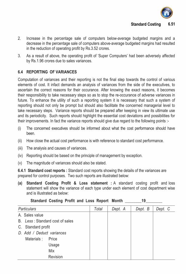
Standard Costing 6.51
2. Increase in the percentage sale of computers below-average budgeted margins and a decrease in the percentage sale of computers above-average budgeted margins had resulted in the reduction of operating profit by Rs.3.52 crores.
3. As a result of above, the operating profit of ‘Super Computers’ had been adversely affected by Rs.1.96 crores due to sales variances.
6.4 REPORTING OF VARIANCES Computation of variances and their reporting is not the final step towards the control of various elements of cost. It infact demands an analysis of variances from the side of the executives, to ascertain the correct reasons for their occurance. After knowing the exact reasons, it becomes their responsibility to take necessary steps so as to stop the re-occurance of adverse variances in future. To enhance the utility of such a reporting system it is necessary that such a system of reporting should not only be prompt but should also facilitate the concerned managerial level to take necessary steps. Variance reports should be prepared after keeping in view its ultimate use and its periodicity. Such reports should highlight the essential cost deviations and possibilities for their improvements. In fact the variance reports should give due regard to the following points :- (i) The concerned executives should be informed about what the cost performance should have
been. (ii) How close the actual cost performance is with reference to standard cost performance. (iii) The analysis and causes of variances. (iv) Reporting should be based on the principle of management by exception. (v) The magnitude of variances should also be stated. 6.4.1 Standard cost reports : Standard cost reports showing the details of the variances are prepared for control purposes. Two such reports are illustrated below: (a) Standard Costing Profit & Loss statement : A standard costing profit and loss
statement will show the variance of each type under each element of cost department wise and is illustrated as below:
Standard Costing Profit and Loss Report Month ________19________
Particulars Total Dept. A Dept. B Dept. C A. Sales value B. Less : Standard cost of sales C. Standard profit D. Add / Deduct variances
Materials : Price Usage Mix
Revision

Advanced Management Accounting 6.52
Labour : Rate of pay Efficiency
Overhead : Efficiency Calendar Capacity Expense
Total E. Actual profit
The adverse variance may be shown in red or in parenthesis. (b) Material usage variance report : This report is sent to the heads of departments for necessary corrective action. A typical report is as under:
Material Usage Variance Report - Dept. A Month______19 ________
Standard Actual This month’s Cumulative Material requirement consumption- variance variance Qty. Value Qty. Value Kgs. Kgs. Kgs. Rs. Kgs. Rs.
A 1,200 1,100 100 100 400 400 B 1,800 2,000 (200) (100) 200 100 C 4,100 4,000 100 200 (500) (1000) D 1,000 950 50 25 75 38 Total 225 (462)
6.4.2 Preparation of Original Budget, Standard Product Cost Sheet and the Reconciliation of Budgeted Profit and Actual Profit : Generally, under variance analysis we compute various variances from the actual and the standard/budgeted data. Sometimes all or a few variances and actual data are made available and from that we are required to prepare standard product cost sheet, original budget and to reconcile the budgeted profit with the actual profit. Preparation of these statements is illustrated below : Illustration 19 The budgeted output of a single product manufacturing company for the year ending 31st March was 5,000 units. The financial results in respect of the actual output of 4,800 units achieved during the year were as under:
Rs. Direct material 29,700

Standard Costing 6.53
Direct wages 44,700 Variable overheads 72,750 Fixed overheads 39,000 Profit 36,600 Sales 2,22,750 The standard wage rate is Rs. 4.50 per hour and the standard variable overhead rate is Rs. 7.50 per hour. The cost accounts recorded the following variances for the year:
Variances Favourable Adverse Rs. Rs.
Material price – 300 Material usage – 600Wage rate 750 –Labour efficiency – 2,250Variable overhead expenses 3,000 –Variable overhead efficiency – 3,750Fixed overhead expense – 1,500Selling price 6,750 –
Required: (i) Prepare a statement showing the original budget. (ii) Prepare the standard product cost sheet per unit. (iii) Prepare a statement showing the reconciliation of originally budgeted profit and the
actual profit. Solution Working Notes :
Rs.
(a) Actual sales 2,22,750 Less : Price variance (Favourable) 6,750 Standard sales 2,16,000 Units sold 4,800
Budgeted price per unit: =
=Rs. 2,16,000 Rs. 454,800 units

Advanced Management Accounting 6.54
(b) Material used 29,700 Rs. Less :Price variance (Adverse) 300
Usage variance (Adverse) 600 900Standard cost 28,800
Standard material cost per unit: = =Rs. 28,800 Rs. 64,800 units
(c) Direct wages spent 44,700 Add: Wage rate variance (Favourable) 750
45,450 Less: Efficiency variance (Adverse) 2,250
Standard wages 43,200
Standard wage rate per unit: =Rs. 43,200 Rs. 94,800 units
(d) Standard direct wage rate is Rs.4.50 per hour. Hence standard time per unit: Rs. 9 ÷ 4.50 hour = 2 hours
(e) Variable overheads : Standard rate Rs.7.50 per hour Variable overhead per unit: 2 hrs. × Rs.7.50 = Rs. 15
(Note : Alternatively, this may be calculated by adjusting variances as in other cases). (f) Fixed overhead spent Rs.39,000 Less : Fixed overhead expense variance (Adverse) Rs.1,500
Budgeted overheads Rs. 37,500
Std. fixed overhead rate per unit : =Rs. 37,500 Rs. 7.50
5,000 units (g) Fixed overhead recovered: 4,800 units × Rs.7.50 = Rs.36,000 (h) Fixed overhead volume variance Rs.36,000 – Rs.37,500 = Rs.1,500 (Adverse) (i) Budgeted sales: 5,000 units × Rs.45 = Rs.2,25,000 (j) Standard sales: 4,800 units × Rs.45 = Rs.2,16,000

Standard Costing 6.55
(k) Actual sales = Rs.2,22,750 (1) Sales volume variance: = Rs.9,000 (Adverse) Rs. 2,16,000 – Rs.2,25,000 (m) Sales price variance:
Rs.2,22,750 – Rs.2,16,000 = Rs. 6,750 (Favourable)
(i) Original budget: Rs.Budgeted sales : (A) (5,000 units × Rs.45) 2,25,000Budgeted costs Direct material (5,000 units × Rs.6) 30,000Direct wages (5,000 units × Rs.9) 45,000Variable overheads (5,000 units × Rs.15) 75,000Fixed overheads (5,000 units × Rs.7.50) 37,500Total budgeted costs : (B) 1,87,500Profit : (A) – (B) 37,500
(ii) Standard product cost sheet per unit Rs.
Direct materials 6.00 Direct wages 9.00 Prime cost 15.00 Variable overheads 15.00 Fixed overheads 7.50 Total cost 37.50 Profit 7.50 Selling price 45.00
(iii) Statement showing Reconciliation of the original Budgeted Profit and the Actual Profit. Rs. R s . Budgeted profit 37,500 Less: Sales margin volume variance (Adverse)*
or loss of profit on sales volume variance
= × 2Rs. 9,000 16 % * *3 1,500
Standard profit 36,000

Advanced Management Accounting 6.56
*Sales margin volume variance (Adverse) (200 units × Rs.7.50 = Rs.1,500)
**Profit as % of selling price : × =100 2Rs. 7.50 16 %
65 3 Add : Sales price variance (Favourable) 6,750 42,750 Add: Favourable cost variances:
Wage rate 750 Variable overhead expenses 3,000 3,750
Less : Adverse cost variances 46,500 Material price 300 Material usage 600 Labour efficiency 2,250 Variable overhead efficiency 3,750
Fixed overhead expense 1,500 8,400 38,100
Less: Fixed overhead volume variance (Adverse) 1,500 [See working note (h)]
36,600 Illustration 20 Jumbo Enterprises manufactures one product, and the entire product is sold as soon as it is produced. There are no opening or closing stocks and work-in-progress is negligible. The company operates a standard costing system and analysis of variances is made every month. The standard cost card for the product is as follows :–
Rs. Direct material 0.5 kgs. at Rs. 4 per kg. 2.00 Direct wages 2 hours at Rs. 2 per hour 4.00 Variable overheads 2 hours at Re. 0.30 per hour 0.60 Fixed overheads 2 hours at Rs. 3.70 per hour 7.40 Standard cost 14.00 Standard profit 6.00 Standard selling price 20.00

Standard Costing 6.57
Selling and administration expenses are not included in the standard cost, and are deducted from profit as a period cost. Budgeted output for April 1997 was 5,100 units. Actual results for April 1997 were as follows : Production of 4,850 units was sold for Rs. 95,600 Material consumed in production amounted to 2,300 kgs. at a total cost of Rs. 9,800. Labour hours paid for amounted to 8,500 hours at a cost of Rs. 16,800. Actual operating hours amounted to 8,000 hours. Variable overheads amounted to Rs. 2,600. Fixed overheads amounted to Rs. 42,300. Selling and administration expenses amounted to Rs. 18,000. You are required to (a) Calculate all variances. (b) Prepare an operating statement for the month ended 30th April 1997. Solution (a) Calculation of Variances: (i) Material price variance = Actual quantity (Std. rate – Actual rate) = Rs. 9,200 – Rs. 9,800 = Rs. 600 (A) (ii) Material usage variance = Std. rate (Std. quantity – Actual quantity) = Rs. 4 (2,425 kg. – 2,300 kg.) = Rs. 500 (F) (iii) Labour rate variance = Actual hours (Std. rate – Actual rate) = Rs. 17,000 – Rs. 16,800 = Rs. 200 (F) (iv) Labour efficiency variance = Std. rate (Std. hours – Actual hours) = Rs. 2 (9,700 – 8,000) = Rs. 3,400 (F) (v) Labour idle time variance = Std. rate × Idle time = Rs. 2 × 500 hrs = Rs. 1,000 (A) (vi) Variable overheads expenditure variance = (Budgeted variable overheads –Actual variable overheads) = ( 8,000 hrs. × Re. 0.30) – Rs. 2,600.

Advanced Management Accounting 6.58
= Rs. 200 (A) (vii) Variable overheads efficiency variance: = Std. rate (Std. hours – Actual hours) = Re. 0.30 (9,700 – 8,000) = Rs. 510 (F) (viii) Fixed overhead expenditure variance : = (Budgeted fixed overheads – Actual fixed overheads) = (5,100 units × Rs. 7.40) – Rs. 42,300 = Rs. 4,560 (A)
(ix) Fixed overheads volume variance: = Budgeted fixed overheads per unit (Budgeted volume – Actual volume) = Rs. 7.40 (5,100 units – 4,850 units) = Rs. 1,850 (A)
(x) Fixed overheads efficiency variance : = Budgeted fixed overheads per hour (Std. hrs. – Actual hrs.) = Rs. 3.70 (9,700 hrs. – 8,000 hrs.)
= Rs. 6,290 (F)
(xi) Fixed overheads capacity variance: = Budgeted fixed overheads per hour (Budgeted capacity – Actual capacity) = Rs. 3.70 {(5,100 × 2) – 8,000)} = Rs. 8,140 (A)
(xii) Sales price variance = Actual qty. (Budgeted rate – Actual rate) = Rs. 97,000 – Rs. 95,600 = Rs. 1,400 (A) (xiii) Sales volume variance = Std. profit per unit (Budgeted sales volume – Actual sales volume) = Rs. 6 (5,100 – 4,850)

Standard Costing 6.59
= Rs. 1,500 (A) (b) Operating Statement for the month ended 30th April 1997 :
Budgeted profit before selling & R s .
R s .
administration expenses (5,100 units × Rs. 6) 30,600 Sales variances : Price 1400(A) Volume 1500(A) 2,900(A) Actual sales minus standard cost of sales 27,700 Cost variances: (F) (A) Rs. Rs. Material price – 600 Material usage 500 – Labour rate 200 – Labour efficiency 3,400 – Labour idle time – 1,000 Variable overheads expenditure – 200 Variable overheads efficiency 510 – Fixed overheads expenditure – 4,560 Fixed overheads efficiency 6,290 – Fixed overheads capacity – 8,140 10,900 14,500 3,600 (A)
Actual profit before selling & administration expenses 24,100 Less: Selling & administration expenses 18,000 Actual profit for the month 6,100 Note: A = Adverse F = Favourable. Check (Not required) : Rs. Rs. Sales 95,600 Less : Cost of materials 9,800 Labour 16,800 Variable overheads 2,600
Fixed overheads 42,300 Selling &Adm. expenses 18,000 89,500
Net profit 6,100

Advanced Management Accounting 6.60
Illustration 21 The working results of a company for two corresponding years are shown below: Year 1 Year 2 Rs. in lakhs Rs. in lakhs
Sales 1,200 1,540Direct Material 600 648 Direct Wages and Variable Overheads 360 412 Fixed Overheads 160 300 1,120 1,360Profit 80 180
In year 2, there has been an increase in the selling price by 10%. Following are the details of material consumption and utilization of direct labour hours during the two years.
Year 1 Year 2
Direct Material Consumption in m/t 5,00,000 5,40,000Direct Labour Hours 75,00,000 80,00,000
You are required to : (i) Keeping year 1 as base year, analyse the results of year 2 and work out the amount
which each factor has contributed to change in profit. (ii) Find out the break even sales for both years. (iii) Calculate the percentage increase in selling price that would be needed over the sale
value of year 2 to earn a margin of safety of 45%. Solution (i) Reconciliation statement showing which factor has contributed change in profit (Rs. in lacs) Favourable Adverse Increase in contribution due to increase in volume (Rs.280 lacs – Rs.240 lacs) 40 — (Refer to working note 3) Sales price variance 140 (Refer to working note 3)

Standard Costing 6.61
Material usage variance 52 (Refer to working note 4) Material price variance — 0 (Refer to working note 4) Direct labour rate variance — 28 (Refer to working note 4) Direct labour efficiency variance 36 — (Refer to working note 4) Fixed overhead expenditure variance
(Refer to working note 3) — 140 268 168
Total change in profit 100
(ii) Break-even sales (Year 1) = Fixed cos tP / V ratio
(Refer to working note 3) Break-even sales (Year 2) (Refer to working note 3)
= . 300
. 480 100.1,540
Rs lacsRs lacsRs lacs
×
= Rs. 962.50 Lacs
(iii) Percentage increase in selling price needed over the sales value of year 2 to earn a margin of safety of 45% in year 2.
P/V ratio = (Rs. 480 lacs/Rs. 1,540 lacs) × 100 = 31.169%
Break-even sales = × =Rs. 962.50 lacs 100 62.5%Rs. 1,540 lacs
(as % to sales)
If Margin of safety to be earned is 45% then Break-even point should be 55%
Contribution increase required = × × =62.5 31.169 100 35.4193%55
Revised contribution = 1,540 lacs × 35.4193% = 545.45 lacs Present contribution = Rs. 480 lacs Increase in selling price required = Rs. 65.45 lacs (Rs. 545.45 lacs – Rs. 480 lacs)

Advanced Management Accounting 6.62
Percentage increase in selling price
over the sales value of year 2 =
× =Rs. 65.45 lacs 100 4.25%
Rs. 1,540 lacs Working notes :
1. Budgeted sales in year 2
If actual sales in year 2 is Rs. 110 then budgeted sales is Rs. 100.
If actual sales in year 2 is Re.1 then budgeted sales =
Rs. 100Rs. 110
If actual sales in year 2 are Rs.15,40,00,000 then budgeted sales are
=
×Rs. 100 Rs. 15,40,00,000 = Rs.1,400 Lacs.Rs. 110
2. Budgeted figures of direct material; direct wages; and variable overhead worked out on the basis of % of sales in year 2 :
Direct material cost
Direct material % to sales (in year 1) = Sales × 100
=
× =600 100 50%
1,200 Budgeted figure of direct
material (in year 2) = 50% × Rs. 1,400 lacs = 700 lacs
Direct wages and variable overhead = Direct wages and var iable overhead
(% to sales in year 1) Sales
=
× =360 100 30%
1,200 Budgeted figure of direct wages
and variable overhead (in year 2) = 30% × 1,400 lacs = 420 lacs
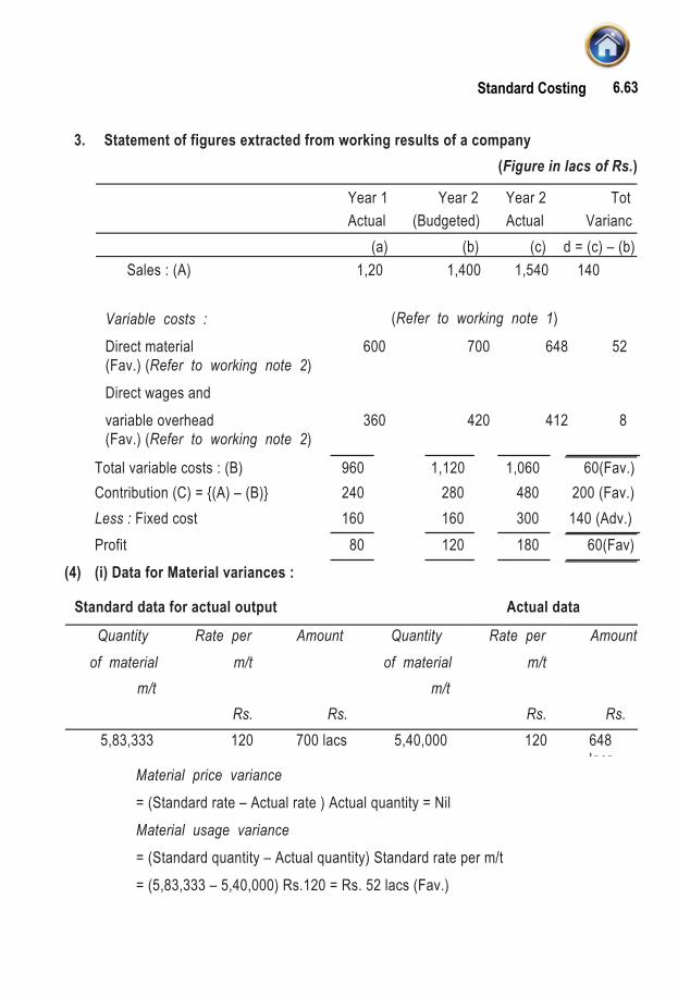
Standard Costing 6.63
3. Statement of figures extracted from working results of a company (Figure in lacs of Rs.)
Year 1 Year 2 Year 2 Tot Actual (Budgeted) Actual Varianc (a) (b) (c) d = (c) – (b)
Sales : (A) 1,20 1,400 1,540 140
Variable costs : (Refer to working note 1)
Direct material 600 700 648 52 (Fav.) (Refer to working note 2) Direct wages and variable overhead 360 420 412 8 (Fav.) (Refer to working note 2)
Total variable costs : (B) 960 1,120 1,060 60(Fav.) Contribution (C) = {(A) – (B)} 240 280 480 200 (Fav.) Less : Fixed cost 160 160 300 140 (Adv.) Profit 80 120 180 60(Fav)(4) (i) Data for Material variances :
Standard data for actual output Actual data
Quantity Rate per Amount Quantity Rate per Amountof material m/t of material m/t
m/t m/t Rs. Rs. Rs. Rs.
5,83,333 120 700 lacs 5,40,000 120 648 lacs
Material price variance = (Standard rate – Actual rate ) Actual quantity = Nil Material usage variance = (Standard quantity – Actual quantity) Standard rate per m/t = (5,83,333 – 5,40,000) Rs.120 = Rs. 52 lacs (Fav.)

Advanced Management Accounting 6.64
(ii) Data for labour variances overhead variances Standard data for actual output Actual data
Labour Rate per Amount Labour Rate per Amount hours Hour hours hour
Rs. Rs. Rs. Rs.
87,50,000 4.80 4.20 lacs 80,00,000 5.15 412 lacs Labour rate variance : = (Standard rate – Actual rate) Actual labour hours = (Rs.4.80 – Rs.5.15) 80,00,000 = Rs. 28 lacs (Adv.) Labour and variable overhead efficiency variance : = {Standard labour hours – Actual labour hours} × Standard rate per hour = {87,50,000 – 80,00,000} Rs. 4.80 = Rs. 36 lacs (Adv.)
Illustration 22 Ravi, Richard, Rahim and Roop Singh are regional salesmen distributing the product of Super Perfumes Ltd. The selling price of the product is Rs. 400 per unit. The sales quota and the standard selling expenses for the year are : -
Salesmen Sales quota Standard selling expenses Rs. Rs. Ravi 7,50,000 2,25,000 Richard 9,00,000 2,47,500 Rahim 11,50,000 2,87,500 Roop Singh 6,00,000 2,25,000 Actual data for the year were as follows : -
Ravi Richard Rahim Roop Singh Days on field work 200 175 225 250Kilometres covered 20,000 18,000 18,000 30,000 Rs. Rs. Rs. Rs.Sales 8,00,000 10,00,000 10,50,000 5,20,000Salary 80,000 80,000 80,000 80,000Free samples 9,000 7,500 5,375 8,000Postage and stationery 8,000 9,000 10,000 6,000Other expenses 9,000 5,000 4,000 10,000

Standard Costing 6.65
The salesmen are allowed conveyance allowance of Rs. 1.50 per kilometre and a daily allowance of Rs. 80 per day for the days spent on field work. Ravi gets a commission of 6 percent on sales and others are given a commission of 5 percent on sales. Corporate sales office expenses are chargeable at the rate of Rs. 30 per unit sold in the case of Ravi and Richard and Rs. 40 per unit in the case of Rahim and Roop Singh. Prepare a schedule showing the selling cost variances by salesmen. Solution (b) Working notes:
Ravi Richard Rahim Roop Singh(i) Standard sales units : 1,875 2,250 2,875 1,500 Sales quota ÷ Rs. 400 (ii) Standard selling expenses per unit (Rs.) 120 110 100 150 (Std. selling expenses/Std. sales units) (iii) Actual sales units : 2,000 2,500 2,625 1,300 Actual sales ÷ Rs. 400 (iv) Actual selling costs Rs. Rs. Rs. Rs. Daily allowance 16,000 14,000 18,000 20,000 Conveyance allowances 30,000 27,000 27,000 45,000 Salaries 80,000 80,000 80,000 80,000 Free samples 9,000 7,500 5,375 8,000 Postage & stationery 8,000 9,000 10,000 6,000 Other expenses 9,000 5,000 4,000 10,000 Commission on sales 48,000 50,000 52,500 26,000 Corporate sales office expenses 60,000 75,000 1,05,000 52,000
Total actual selling cost 2,60,000 2,67,500 3,01,875 2,47,000
(v) Standard selling cost 2,40,000 2,75,000 2,62,500 1,95,000 (Actual units sold × Std. selling expenses per unit)

Advanced Management Accounting 6.66
Since all the selling expenses have been related to sales units, only one variance can be calculated by comparing the standard and actual selling costs as is shown in the schedule below:
Schedule showing the selling cost variances by salesman Total
Rs. Rs. Rs. Rs. Rs. Standard selling
expenses (Refer to Working Note (v)) 2,40,000 2,75,000 2,62,500 1,95,000 9,72,500 Actual selling expenses (Refer to Working Note (iv)) 2,60,000 2,67,500 3,01,875 2,47,000 10,76,375 Selling cost variance (20,000) 7,500 (39,375) (52,000) (1,03,875)
(A)(F) (A) (A) (A)
A = Adverse F = Favourable
6.5 ACCOUNTING PROCEDURE FOR STANDARD COST The standard cost operations can be recorded in the books of account. Two important accounting procedures for standard costs are :- 6.5.1 Partial plan : This system uses current standards in which the inventory will be valued at current standard cost figure. Under this method the work-in-progress account is charged at the actual cost of production for the month and is credited with the standard cost of the month’s production of finished product. The closing balance of work-in-progress is also shown at standard cost. The balance after making the credit entries represent the variance from standard for the month. The analysis of the variance is done after the end of the month. This method is simple in operation because variances are analysed after the end of month but may present difficulties if the firm makes a variety of products. The following illustration will explain the operation of the recording of standard cost under this method. Illustration 24 Material purchased 10,000 pieces at Rs. 1.10 Rs. 11,000 Materials consumed 9,500 pieces at Rs. 1.10 Rs. 10,450 Actual wages paid 2,475 hours at Rs. 3.50 Rs. 8,662.50 Actual factory expenses incurred Rs. 17,000 (Budgeted Rs. 16,500) Units produced: 900 units and sold at Rs. 60 per unit. The standard rates and prices are as under: Direct materials Re. 1.00 per unit Standard input 10 pieces per unit

Standard Costing 6.67
Direct labour rate Rs. 3.00 per hour Standard requirement 2.5 hours per unit Overheads Rs. 6.00 per labour hour Solution (A) The cost sheet for 900 units will appear as under :
Cost Std. qty. Std. rate Std.cost Rs. Direct material 9,000 1.00 9,000 Direct labour 2,250 3.00 6,750 Overheads 2,250 6.00 13,500 29,250
(B) Calculation of variances: Material price variance = 9,500 Pcs. (Re. 1.00 – Rs.1.10) = Rs. 950 (A) Material usage variance = Re. 1.00 (9,000 pcs. – 9,500 pcs.) = Rs. 500 (A) Labour rate variance = 2,475 hrs. (Rs. 3.00 – Rs. 3.50) = Rs. 1,237.50 (A)
Labour efficiency variance = Rs. 3.00 (2,250 hrs. – 2,475 hrs.) = Rs. 675(A) Overhead variances : (a) Charged to production as per cost sheet Rs. 13,500 (b) Actual hours × Std. rate: 2,475 hrs. × Rs. 6 Rs. 14,850 (c) Overheads as per budget Rs. 16,500 (d) Actual overheads Rs. 17,000
Efficiency variance : (a – b) Rs. 1,350 (A) Capacity variance : (b – c) Rs.1,650 (A) (idle time) Expense variance : (c – d) Rs. 500 (A) Total variance : (a – d) Rs. 3,500 (A)

Advanced Management Accounting 6.68
(C) The. journal entries for recording these transactions are as under : Dr. Cr Rs. Rs. (i) Material Control A/c Dr. 11,000
To General Ledger Adjustment A/c 11,000 (Being the purchase value of 10,000 pieces of materials at Rs. 1.10 each) (ii) Work-in-Progress A/c Dr. 10,450 To Material Control A/c 10,450 (Being the cost of 9,500 pieces of materials actually issued to production at the actual price of Rs. 1.10 each) (iii) Work-in-Progress A/c Dr. 8,662.50 To Wages Control A/c 8,662.50 (Being the actual amount of direct wages paid for 2,475 hours at Rs. 3.50 per hour, (iv) Work-in-Progress A/c Dr. 17,000 To Overhead Expense Control A/c 17,000 (Being the actual overhead expenses incurred) (v) Finished Stock Control A/c Dr. 29,250 To Work-in-Progess A/c 29,250 (Being the standard cost of production transferred to finished goods account) (vi) Cost of Sales A/c Dr. 29,250 To Finished Stock Control A/c 29,250 (Being the standard cost of goods sold transferred to Cost of Sales A/c)
After the basic transactions are posted, the materials control account will show the actual value of stock of material in hand and the work-in-progress account will show a balance representing the cumulative variances on all the accounts and closing balance of work-in- progress at standard cost. The variances have already been analysed in Para (B) above

Standard Costing 6.69
and they will be carried to the respective accounts pending investigation before being finally disposed off. In this problem we have assumed that there is no closing balance of work-in- progress. (D) The journal entries for transferring the variances to their respective accounts
are as under
Rs. Rs. Material price variance A/c Dr. 950.00 Material usage variance A/c Dr. 500.00 Labour rate variance A/c Dr. 1,237.50 Labour efficiency variance A/c Dr. 675.00 Overhead efficiency variance A/c Dr. 1,350.00 Overhead capacity variance A/c Dr. 1,650.00 Overhead expense variance A/c Dr. 500.00
To work-in-progress A/c 6,862.50 (E) The ledger accounts will appear as under:
Dr. Material Control A/c Cr. Rs. Rs. To Opening balance - By Work-in-Progress A/c 10,450 To General Ledger By Balance c/d 550 Adjustment A/c 11,000 11,000 11,000
Work-in-Progress Control A/c
Rs. Rs.To Opening balance – By Finished stock control A/c 29,250.00To Material control A/c 10,450.00 By material price variance A/c 950.00To Wages control A/c 8,662.50 By material usage variance A/c 500.00To Overheads control A/c 17,000.00 By labour rate varianve A/c 1,237.50 By labour efficiency variance A/c 675.00 By overhead efficiency A/c Variance A/c 1,350.00 By overhead capacity Variance A/c . 1,650.00 By overhead expense Variance A/c 500.00 36,112.50 36,112.50

Advanced Management Accounting 6.70
6.5.2 Single Plan : The main purpose of standard costing is cost control. To achieve this purpose, the variances should be analysed according to their causes. Analysis should be timely so that much time is not lost in taking corrective action wherever needed. In the partial plan, we have seen that the variances are analysed at the end of period. The single plan system envisages the posting of all items in the debit side of the work-in-progress account at the standard cost leaving the credit side to represent the standard cost of finished production and work-in-progress. This system enables the ascertainment of variances as and when the transaction is posted to work-in-progress account. In other words, the analysis of variances is done from the original documents like invoices, labour sheets, etc., and this method of analysis is known as analysis at source. Since, the single plan system contemplates the analysis of variances at source, the installation of this system requires more planning so that effective documentation at each stage is introduced for proper recording and analysis of variance. Thus for example, the issue of bill of materials to the stores enables the storekeeper to calculate the standard value of materials. If any material is requisitioned beyond the standard, he can mark the same for material usage variance account. In the production department, as and when the finished output is recorded, the standard waste and actual waste can be compared and necessary entries can be made by the shop supervisors for posting the excessive usage to appropriate variance accounts. Scheme of entries : So far as materials are concerned, material price variances are recorded at the time of receipt of the material and the material quantity variances are recorded as far as possible when excess materials are used. The entries will be as illustrated below: 1. Dr. Material Control A/c Dr. or Cr. Material Price Variance A/c Cr. Creditors A/c. This entry enables the firm to debit the material control account with the actual purchases at
standard cost and credit the creditor ’s account at the actual cost of actual prices thereby transferring the variances to price variance account.
2. Dr. Work-in-progress Control A/c Dr. or Cr. Material Usage Variances A/c Cr. Material Control A/c This entry charges the work-in-progress control account with the standard cost of standard quantity and credit the material control account at the standard cost of actual issue, the variance being transferred to usage variance account. 3. Dr. Wages Control A/c Dr./Cr. Labour Rate Variances A/c Cr. Cash

Standard Costing 6.71
This entry is passed to record the wages at standard rate thereby transferring rate variances to the appropriate account. 4. Dr. Work-in-progress Control A/c Dr. or Cr. Overhead Expense Variances A/c Cr. Overhead Expense Control A/c. The complete procedure in recording the transactions under this system is given in the following illustration: Illustration 25
Standard cost sheet per unit output is as under Rs. Direct material 3 pcs. @ Rs. 2.15 6.45 Direct Labour: Dept. A 2 hrs @ Rs. 1.75 3.50 Dept. B 4 hrs. @ Rs. 1.50 6.00 9.50 Overheads : Dept. A 2 hrs. @ Re. 0.50 1.00 Dept. B 4 hrs. @ Re. 1.00 4.00 5.00 20.95
Transactions for the period are as under : Materials purchased and consumed:
8,600 pcs. @ Rs. 2.50 each Labour time spent
Dept. A. 5,200 hours Dept. B. 12,000 hours
There is no change in labour rates. Actual factory overheads are :
Dept. A. Rs. 3,000 Dept B. Rs. 12,500
Units produced: Dept. A. 2,800 Dept. B. 2,800

Advanced Management Accounting 6.72
Budgeted overheads: Dept. A. Rs. 3,000 Dept. B. Rs. 12,000
Solution (A) Computation of variance:
(i) Material price variance: 8,600 pcs. (Rs. 2.15 – Rs. 2.50) = Rs. 3,010 (A) (ii) Material usage variance: Rs. 2.15 (8,400 Pcs. – 8,600 Pcs.) = Rs. 430 (A)
[Standard requirement of materials = 2,800 units produced × 3 pcs. per unit = 8,400 pcs.]
(iii) Labour efficiency variance: Dept. A: Standard time required = 2,800 pcs. × 2 hrs. = 5,600 hours. Dept. B: Standard time required = 2,800 pcs. × 4 hrs. = 11,200 hours.
Variances : Dept. A: 1.75 (5,600 – 5,200) = Rs. 700 (F) Dept. B: 1.50 (11,200 – 12,000) = Rs. 1,200 (A)
(iv) Overheads variances: (a) Charged to production: Dept. A Dept. B Total Rs . Rs . Rs. Dept. A. 5,600 × 0.50 2,800 Dept. B. 11,200 × 1.00 11,200 14,000 (b) Actual hours at std. rate : Dept. A. 5,200 × 0.50 2,600
Dept. B. 12,000 × 1.00 12,000 14,600 (c) Budgeted overheads 3,000 12,000 15,000
(d) Actual expense 3,000 12,500 15,500 Efficiency variance : (a – b) 200(F) 800(A) 600(A) Capacity variance : (b – c) 400(A) – 400(A) Expense variance : (c – d) – 500(A) 500(A) Total variance : (a – d) 200(A) 1,300(A) 1,500(A)

Standard Costing 6.73
(B) Journal entries :
Dr. Cr. Rs. Rs.
(i) Material Control A/c Dr. 18,490 Material price variance A/c Dr. 3,010 To Creditors A/c 21,500 (ii) Work-in-Progress Dept. A. A/c Dr. 18,060 Material usage variance A/c Dr. 430 To Material Control A/c 18,490 (iii) Work-in-progress Dept. A. A/c Dr. 9,800 To wages control A/c 9,800 (iv) Wages Control A/c Dr. 700 To Labour Efficiency Variance Dept A A/c 700 (v) Work-in-Progress Dept. B A/c. Dr. 16,800 Labour Efficiency Variance Dept. B A/c Dr. 1,200 To Wages Control A/c 18,000 (vi) Work-in-Progress Dept. A A/c Dr. 2,800 Overhead Capacity Variance Dept. A. A/c Dr. 400 To Overhead Efficiency Variance Dept. A. A/c 200 To Overhead Expense Control Dept. A A/c 3,000 (vii) Work-in-Progress Dept. B A/c Dr. 11,200 Overhead Efficiency Variance A/c Dr. 800 Overhead Expenses Variance A/c Dr. 500 To Overhead Control Dept. B A/c 12,500 (viii) Work-in-Progress Dept. B A/c Dr. 30,660 To Work-in-Progress Dept. A A/c 30,660 (Being the transfer at standard cost of finished Production of Department A to Department B for processing in Department B) (ix) Finished Stock control A/c Dr. 58,660 To Work-in-Progress Dept. B A/c 58,660

Advanced Management Accounting 6.74
(C) Ledger Accounts: Dr. Material Control A/c Cr.
Rs. Rs. To Creditors 18,490 By Work-in-Progress (Dept. A) A/c 18,060 By Material usage variance A/c 430 18,490 18,490
Dr. Wages Control A/c Cr. Rs. Rs. To Cash By Work-in-Progress (Dept. A) A/c 9,800 (or Wages payable A/c) 27,100 By Work-in-Progress (Dept. B)A/c 16,800 To Labour efficiency 700 By Labour efficiency variance Variance (Dept, A) A/c (Dept. B) A/c 1,200 27,800 27,800
Dr. Work-in-Progress (Dept. A) Control A/c Cr. Rs. Rs. To Material Control A/c 18,060 By Work-in-Progress (Dept.B) A/c 30,660 To Wages Control A/c 9,800 To Overhead Control 2,800 (Dept. A) A/c 30,660 30,660
Dr. Work-in-Progress (Dept. B) Control A/c Cr. Rs. Rs. To Work-in-Progress By Finished Stock.Control A/c 58,660 (Dept. A) A/c 30,660 To Wages Control A/c 16,800 To Overhead Control (Dept. B) A/c 11,200 58,660 58,660
Dr. Overhead Expense Control (Dept. A) A/c Cr. Rs. Rs.To Cash 3,000 By Work-in-Progress (Dept. A) A/c 2,800To Overhead Efficiency 200 By Overhead Capacity Variance A/c 400Variance A/c
3,200 3,200

Standard Costing 6.75
Dr. Material Price Variance A/c Cr. Rs. Rs. To Creditros 3,010 By Costing P & L A/c 3,010
Dr. Material Usage Variance A/c Cr. Rs. Rs.
To Material Control A/c 430 By Costing P & L A/c 430
Dr. Labour Efficiency Variance A/c Cr. Rs. Rs.
To Wages Control A/c 1,200 By Wages Control A/c 700(Efficiency of Dept. B) By Costing P & L A/c 500
1,200 1,200
Dr. Overhead Efficiency Variance A/c Cr. Rs. Rs. To Overhead Expenses By Overhead Exp. Control Control (Dept. B) A/c 800 (Dept. A) A/c 200 By Costing P & L A/c 600 800 800 Dr. Overhead Capacity Variance A/c Cr.
Rs. Rs. To Overhead Expenses 400 By Costing P & L A/c 400
Control (Dept. A) A/c Dr. Overhead Expenses Variance A/c Cr. Rs. Rs. To Overhead Expenses 500 By Costing P & L A/c 500 Control (Dept. B) A/c Dr. Creditors A/c Cr. Rs. Rs. To Balance 21,500 By Material Control A/c 18,490 By Material Variance A/c 3,010 21,500 21,500

Advanced Management Accounting 6.76
Dr. Overhead Expenses Control (Dept ‘B’) A/c Cr. Rs. Rs. To Cash 12,500 By Work-in-Progress Dept. A A/c 11,200 By Overhead Efficiency Variance (Dept. B) A/c 800 By Overhead Expenses Variance 500 (Dept. B) A/c 12,500 12,500 Dr. Finished Stock Control A/c Cr.
Rs. Rs. To Work-in-Progress 58,660 By Balance c/d 58,660 Dept. B A/c
Recapitulation : (1) Current standards are used in both the systems. (2) Under the partial plan, material stocks are carried at actual cost whereas the same are
carried out at standard cost under the single plan. (3) The work-in-progress and finished goods are valued at standard cost under both the
methods. (4) Computation of variances :
(a) In partial plan, material price variance is computed on material used in finished goods and work-in-progress whereas in single plan it is computed on the material quantity purchased.
(b) The partial plan is suitable where simple analysis of variance is sufficient at the end of the period whereas the single plan is preferred if frequent detailed analysis of variance is desired, as (a) the comparison of actual with standard cost of each operation or operator or (b) the daily reporting of standard cost of excess material used.
6.6 BEHAVIOURAL ASPECTS OF STANDARD COSTING 1. Projection of fixed overheads and estimated selling price in a Standard Cost Sheet is a
circular exercise with no added value.
In an award winning article,” COST / MANAGEMENT ACCOUNTING: THE 21ST CENTURY PARADIGM”, published in Management Accounting (USA), December 1995, William L Ferrara argues that while preparing a Standard Cost Sheet, one of the objectives of which is to assist management in pricing products, a professional cannot

Standard Costing 6.77
project fixed overheads until and unless he is aware of the production quantum to be effected. The forecast of future production can only be made if a tentative selling price of the product is known because, in a competitive market, it is the selling price which decides the sale quantity and therefore the production volume. The authors contend that in case the selling price is known at the time of projecting fixed overheads then the re computation of the same is a valueless exercise.
2. Traditional costing tools like standard costing induce a static behaviour in the employees. During the past decade and a half, various writers such as Johnson and Kaplan, Ferrara
and Monden etc have questioned the productivity and use of traditional systems such as standard costing and variance analysis. They argue that the use of standard costing renders employees static and curbs innovation and that companies following traditional standard costing find it difficult to improve upon standards because of severe resistance from employees who are convinced that the established best practise cannot be improved further.
3. Fear of adverse variances forces managers to give undue importance to material price, labour rate and efficiency and capacity utilisation. These concepts are detrimental to the modern day world class manufacturing environment characterised by concepts of JIT and TQM.
In a World Class Manufacturing environment, characterised by Just in Time policies, the focus of the management is to produce only as much as is required. This requires purchase of small quantities of raw material, increase in the number of set ups and minimal importance to capacity utilisation. Policies like this result in increased adverse variances related to raw material prices, labour efficiency and production volume. Critics argue that the fear of such adverse variances affects goal congruence and forces managers to behave against their company’s policies.
4. Traditional costing does not provide the management with what is the allowable cost; rather it emphasises on the standard or actual costs. This is looked upon as one of the major reasons for lack of innovation especially in the global era where competition amongst companies is unprecedented. It is argued that techniques like Target costing are much more motivating when compared to Traditional costing since the former encourage the use of concepts like value engineering and value analysis.
SELF-EXAMINATION QUESTIONS 1. Fill in the banks :
(a) Compilation of direct material and labour standards entails setting up of —— and —————standards.
(b) Time and motion study is used to set ............ standard. (c) Overhead expense standards are based on the budgeted.......................

Advanced Management Accounting 6.78
(d) A standard hour is a ......... hour meant for.................. (e) Standard costing is necessary for jobbing industry to...........a price and ............ a
profitable job. (f) Standard costing works on the principle of .................... (g) The problem of price fluctuations can be overcome to some extent by the use of
................ techniques. (h) The suitable type of standard for control purposes is ................
2. State whether the following statements are true or false: (a) The industrial engineering department is responsible for setting physical standards. (b) Constant shortage of a material of specified quality in a factory may pose a problem
in setting physical standards. (c) If labour time standard is based on the maximum effciency, the unit cost will be
higher. (d) Setting of overhead expense standards involves the selection of a suitable level of
output and budgeting of expense for that level of output. (e) Where products of different sizes, shapes and quality are manufactured in a factory,
standard hours is the proper basis of comparison of the output. (f) Jobs differ from one another and hence it is not possible to use standard costing in
jobbing industries. (g) Inventory of finished goods for financial accounting purposes should be based on
standard costs adjusted for price or expenditure variances. (h) Standard costing does not help the manager in decision making. (i) Standard costs
help price fixing when demand is elastic. (j) Standard costs reflect optimum operations by bringing economic and technical
factors together. 3. Explain briefly how standards are compiled for material and labour costs for a product 4. Fill in the blanks :
(a) Variance analysis involves the .............and .........................of variances. (b) Broadly variances may be of three types.......................... (c) Selling and distribution expenses can be analysed under ......................... (d) Cost ratios may be useful to control .................. overheads.

Standard Costing 6.79
5. State whether the following statements are true or false: (a) Variances can be classified into controllable and uncontrollable. (b) All price variances are uncontrollable. (c) Operation cost method is not suitable for controlling administration overheads. (d) Work units can be established for measuring the output in relation to cost, to control
selling and distribution costs. 6. In group A, the names of variances are given and in group B, examples of the reasons
for cost variances are given. Match them. Group A Group B A. Material Price Variance. (1) A non-standard mixture used B. Labour Rate Variance. (2) Changes in basic price of raw materials. C. Overhead Volume Variance. (3) Poor working conditions. D. Materials Usage Variance. (4) Using skilled labour in place of unskilled labour. E. Labour Efficiency Variance. (5) Slackness in production 7. Explain briefly the nature and purpose of material and labour variances. 8. Fill in the blanks :
(a) In a textile mill, different varieties of cotton are blended in different proportions. If the blend deviates from the standard blend, we get ..................................... variance.
(b) The relation between the finished product and the raw material input is known as.............
(c) If a skilled workman is used in place of an unskilled workman ...............variance arises.
(d) Volume variance arises because of .................. expenses. 9. Compute the material variances from the following data. Actual quantity consumed 100 Kgs. Actual price per kg. Rs. 19 Standard price per kg. Rs. 20 Production in standard units is 45 units; one standard unit requires 2 kg. of material. 10. The standard time per unit is 2 hours at Re. 1/- per hour. During a period, 500 units are
made and the records showed the actual payment of wages of Rs. 1,800 for 1200 hours worked. Compute the labour cost variances.

Advanced Management Accounting 6.80
11. Given the following data compute the overhead expense variances. Fixed Variable
Actual overheads per month Rs.1,200 Rs.4,000 Budget for 10,000 hours Rs.1,000 Rs.3,500 Standard hours produced 10,400 Actual hours worked 10,000
12. The income statement of XYZ Co. is presented below: XYZ Company
Income statement for the year ended Dec. 31, 1996
Product Product Total AR-10 ZR-7
Budget Actual Budget Actual Budget ActualSales (units) 2,000 2,800 6,000 5,600 8,000 8,400Total sales of market (units) – – – – 40,000 45,654Sales revenue (Rs.) 6,000 7,560 12,000 11,760 18,000 19,320Cost of goods sold (Rs.) 2,400 2,800 6,000 5,880 8,400 8,680Fixed costs (Rs.) 1,800 1,900 2,400 2,400 4,200 4,300Total costs (Rs.) 4,200 4,700 8,400 8,280 12,600 12,980
Net profit (Rs.) 1,800 2,860 3,600 3,480 5,400 6,340Using the above information compute: (a) Market size variance. (b) Market share variance.
13. Fill in the blanks : (a) The three plans of accounting for standards are ..................... (b) In partial system work-in-progress account is credited at ............ cost. (c) In single plan system work-in-progress account is charged at ............ cost. (d) Under dual plan standards are used .............
14. State whether the following statements are true or false. (a) In partial plan, the analysis is made at source.

Standard Costing 6.81
(b) Dual plan helps to express the variances in the form of efficiency indices. (c) Dual plan helps to convert standards into actuals by using the ratios. (d) Single plan uses current standards.
15. The following are the two journal entries for the transaction noted below. State the plan to which these entries are applicable.
(a) Standard Clearing A/c Dr. To Material Control A/c
For charging the actual quantity of material consumed at standard price. (b) Material Control A/c Dr.
Dr. or Cr. Material Control Variance A/c To Creditors
(For charging the standard cost of material to material control account there by transferring the price variance to price variance account.)
16. How are variances disposed off in a standard costing system? Explain. 17. “Calculation of variances in standard costing is not an end in itself, but a means to an
end. “Discuss. 18. GLOBAL LTD. is engaged in marketing of wide range of consumer goods. A, B, C and D
are the zonal sales officers for four zones. The company fixes annual sales target for them individually.
Your are furnised with the following : (1) The standard costs of sales target in respect of A, B, C and D are Rs. 5,00,000,
Rs. 3,75,000, Rs. 4,00,000 and Rs. 4,25,000 respectively. (2) A, B, C and D respectively earned Rs. 29,900, Rs. 23,500, Rs. 24,500 and Rs.
25,800 as commission at 5% on actual sales effected by them during the previous your.
(3) The relevant variances as computed by a qualified cost accountant are as follows:
A B C D Rs. Rs. Rs. Rs.
Sales price variance 4,000 (F) 6,000 (A) 5,000 (A) 2,000 (A) Sales volume variance 6,000 (A) 26,000 (F) 15,000 (F) 8,000 (F)Sales margin mix variance 14,000 (A) 8,000 (F) 17,000 (F) 3,000 (A)
(A) = Adverse variance and (F) = Favourable variance

Advanced Management Accounting 6.82
You are required to : (i) Compute the amount of sales target fixed and the actual amount of contribution
earned in case of each of the zonal sales officer. (ii) Evaluate the overall performance of these zonal sales officers taking three relevant
base factors and then recommend whose performance is the best.
ANSWERS TO SELF - EXAMINATION QUESTIONS 1. (a) quantity price (b) labour time (c) output (d) hypothetical, measuring output. (e) quote,
choose (f) exception (g) forecasting (h) attainable level of good performance. 2. (a)True (b) True (c) False (d) True (e) True(f) False, (g) True, (h) False (i) True (j) True 4. (a) Calculation, interpretation (b) efficiency, price and volume (c) order processing,
warehousing, sales promotion and distribution (d) administration. 5. (a) True (b) False (c) False (d) True 6. A,2 ; B,4 ; C, 5 ; D, 1 ; E, 3. 8. (a) mix (b) yield (c) substitution (d) fixed. 9. Usage variance Rs. 200 (A) Price variance Rs. 100 (F) 10. Efficiency variance Rs. 200 (A) Rate of pay variance Rs. 600 (A) 11. Types of variances
Fixed Variable Efficiency variance Rs. 40(F) Capacity variance Nil Expense variance Rs. 200 (A) Rs. 500 (A) 12. (a) Market size variance; Rs. 1,357 (Favourable) (b) Market share variance; Rs. 877 (Adverse) 13. (a) Partial, single and dual (b) actual (c) standard (d) bogey 14. (a) False (b) True (c) True (d) True. 15. (a) Dual (b) Single
18. (i) Actual margin A B C D Rs. ’000 90 77 92 80
(ii) The performance of the officer C is best.

7 Costing of Service Sector
LEARNING OBJECTIVES : After finishing this chapter, you will be able to understand and appreciate the peculiarities involved in the costing of service sector. Through this chapter you will gain an understanding as to the various methods applied by service sector entities to determine their unit costs.
7.1 INTRODUCTION
Service sector companies provide their customers with services or intangible products. The activities of service sector may be used for both: (i) Provision of services to outside customers (ii) Provision of services internally (i.e. captive consumption). The types of services that may be provided, by service sector are of diverse nature and have their own peculiarities and requirements in respect of the cost accounting treatment, however, the general principles of costing discussed in earlier chapters relating to manufacturing sector also apply to service sector.
7.2 MAIN CHARACTERISTICS OF SERVICE SECTOR
(i) Activities are labour intensive: Due to their inherent nature, the activities of service sector are generally labour intensive. The direct material cost is either small or non-existent. The labour cost (i.e. salary and wages) constitutes a significant portion of the total operating costs of a service sector entity. For example, cost of stationery used by a professional consultant for expressing an opinion in black and white, for a client will be small or even non existent in case he gives verbal opinion. In the preceding example direct labour cost (i.e. the salary of the consultant) constitutes a significant portion of the total operating cost as compared to the material cost which constitutes a negligible portion.
(ii) Cost-unit is usually difficult to define: The selection of cost unit for service sector is relatively difficult to ascertain as compared to the selection of cost unit for manufacturing sector.

Advanced Management Accounting 7.2
The following table provides some examples of the cost units for service sector.
(A) To External Customers Cost Unit
(i) Hotel Bed nights available, Bed night occupied
(ii) School Student hours, Full time students
(iii) Hospital Patient per day, Room per day
(iv) Accounting firm Charged out client hours
(v) Transport Passenger km., quintal km.
(B) Internal services Cost Unit (i) Staff canteen Meals provided, No. of staff
(ii) Machine maintenance Maintenance hours provided to user department
(iii) Computer department Computer time provided to user department
(iii) Product costs in service sector: Costs are classified as product or period costs in manufacturing sector for various reasons viz.
(i) To determine the unit manufacturing costs so that inventories can be valued and the selling prices be determined & verified.
(ii) To report production costs on income statement.
(iii) To analyse costs for control purposes.
The only difference between manufacturing and service sector is that in service sector there is no physical product that can be stored, assembled and valued. Services are rendered and cannot be stored or placed in a vault. In service sector the cost of material is insignificant. Rendering a loan service, representing someone in court of law or selling an insurance policy are typical services performed by professionals. For computing unit cost of these services the most important cost would be professional’s labour cost. The direct labour cost is traceable to service rendered. In addition to labour cost the service sector like manufacturing sector incurs various overhead cost. In service sector those overhead costs which are incurred for offering a service are classified as service overhead (like factory overhead in manufacturing sector). In order to arrive at the correct cost incurred for rendering services, it is imperative that such overheads be allocated/apportioned over the cost units.
7.3 COLLECTION OF COSTING DATA IN SERVICE SECTOR Costs are accumulated under various heads for control purposes and for decision making. Costs thus, collected are usually grouped under fixed costs and variable costs. The format in which costs data is presented depends upon the nature of industry and the need of the

Costing of Service Sector 7.3
management. In the Cost Accounting book of PE-II level we have discussed in the chapter of operating costing the costing methods appropriate for different types of service sector i.e. Transport Sector, Hospital, Hotel, College etc. Often composite cost units such as passenger km, bed, nights etc. are used by these organisation for ascertaining the cost per unit in respect of these services respectively. For preparing a cost sheet under operating costing, costs are usually accumulated for a specified period viz. a month, a quarter or year etc. Since there is no direct relationship between the costs and level of services there is tendency in service sector to view all the costs as over- heads. If such a view is taken the cost control will be achieved by controlling the inputs rather than the outputs i.e. control will be relatively ineffective. This gives an impetus for the application of Activity Based Costing in service sector, with a desire to secure better understanding of costs, as an aid to decision making and cost control. Although the Activity Based Costing was initially developed for manufacturing sector, it can be applied with equal effectiveness to service sector for understanding cost behaviour of service sector entities as well.
7.4 COSTING METHODS USED IN SERVICE SECTOR Like manufacturing sector companies in the service sector, generally adopt one out of the following two basic costing methods to assign costs to services. These are:
1. Job costing method: In job costing method the cost of a particular service is obtained by assigning costs to a distinct identifiable service. In service sector like Accounting firm, Advertising campaigns etc. job costing method is used. For assigning indirect costs (overheads) models such as Activity Based Costing may be used.
2. Process costing method: In process costing system the cost of a service is obtained by assigning costs to masses of similar unit and then computing unit cost on an average basis. Retail banking, Postal delivery, Credit card etc. uses process costing method.
3. Hybrid costing method: Many companies uses a method of costing which is neither job costing nor process costing method. They in fact uses a hybrid costing method which combines elements of both job costing and process costing methods.
The job costing and process costing for manufacturing sector have been discussed in the Cost Accounting book of PE-II level. The same cost principles as discussed for manufacturing sector will apply to service sector.
7.4.1 Job costing method in service sector: The two significant costs which are incurred in service sectors are :
(i) Direct labour
(ii) Service overheads For ascertaining the price of a service provided by service sector if job costing method is followed, the costs for each job are to be monitored continuously. There are two main uses of this job cost information :

Advanced Management Accounting 7.4
1. To guide decisions on job pricing 2. To assist in enhancing profitability by cost planning and cost control The five steps which are generally adopted for assigning costs to individual jobs are as follows:
(i) Identify the job that is chosen as cost object : For instance, litigation work for Motorola India Ltd. by Dua & Associates by assuming that work requires 100 budgeted hours of professional labour.
(ii) Identify the direct cost categories for the job: In the above example the professional hours required for doing litigation work is a direct cost.
(iii) Identify indirect costs (overheads) associated with the job: This step requires identification of indirect costs incurred for providing services. These costs may include the costs of support labour, computer time, travel, telephone/fax machine, photocopying etc.
(iv) Select the cost allocation base to be used in assigning each indirect cost to the job: This step requires the selection of cost allocation base that has a cause and effect relationship between changes in it and changes in the level of indirect costs. The allocation base suitable for allocating indirect cost of law firm is professional labour hours.
(v) Identify the rate per unit of the cost allocation base used to allocate cost to the job: The budgeted indirect cost allocation rate is computed by using following formula
Budgeted total indirect cost Budgeted indirect cost rate =
Budgeted total quantity of cost allocation base The indirect cost of job is computed as = Budgeted indirect cost rate × Professional labour
hours reqd. for job Example Dua and Associates is a law firm specialising in carrying out litigation work for clients. It has 25 professionals who work for clients (5 partners and 20 associates). The average budgeted total compensation per professional for 1999 is Rs. 1,04,000. Each professional is budgeted to have 1,600 billable hours to clients in 1999. Dua and Associates is a highly respected firm and all professionals work for clients to their maximum 1,600 billable hours. All professional labour costs are traceable to jobs on a per hour basis. The budgeted indirect cost (legal support) in 1999 is Rs. 22,00,000. The indirect costs are allocated to the jobs using professional labour hours as the allocation base. In this example for ascertaining the cost of job company consider single direct cost rate (i.e. Professional labour) and single indirect cost rate.
Cost Accumulation
Cost Allocation

Costing of Service Sector 7.5
The job costing method example given above uses single direct cost and single indirect cost for computing the cost of the job. The use of single direct cost and single indirect cost is likely to overstate job with more professional hours and understate the jobs with less professional hours. This requires refinement of costing system. The refinement in costing system means changes in existing costing system that results in a better measure of the way the jobs uses the resources of the organisation. Many organisations in service sector for refining their costing system are using activity based costing (ABC). Activity based costing focusses on activities as the fundamental cost objects. It uses the cost of these activities as the basis for assigning costs of services to jobs. For understanding the implementation of ABC in service sector consider the above example.
In the above example Dua and Associates for refining its costing method reviewed its work activities and collected information about how each litigation work vary in their use of resources. They identified that the direct costs are of the following five categories. These are:
1. Professional Partner labour
2. Professional Associate labour
3. Office support labour.
4. Phone/fax/photocopying : Traced on as identified basis or per monthly billing from third parties.
5. Travel : Traced on as identified basis, per monthly billing from third parties.
Similarly, indirect costs are identified into two categories. These are:
1. General support: The allocation base is budgeted professional labour hours.
2. Out of town support: The allocation base in law firm is lawyer days at non-local site.
With refined costing system service organisation has more accurate cost information for services. This helps them to adjust their pricing policies for services
7.4.2 Process costing method in service sector : In this method the cost of service is obtained by assigning costs to masses of units and then computing unit costs on an average basis. Let us explain this with an illustration.
Illustration
The loan department of a Canara Bank performs several functions in addition to home loan application processing task. It is estimated that 25% of the overhead costs of loan department are applicable to the processing of home-loan application. The following information is given concerning the processing of a loan application :

Advanced Management Accounting 7.6
Direct professional labour :
Rs. Loan processor monthly salary : 80,000 (4 employees @ Rs. 20,000 each) Loan department overhead costs (monthly) Chief loan officer’s salary 5,000 Telephone expenses 750 Depreciation Building 2,800 Legal advice 2,400 Advertising 400 Miscellaneous 650 Total overhead costs 12,000 You are required to compute the cost of processing home loan application on the assumption that one hundred home loan applications are processed each month. Solution:
Statement showing computation of the cost of processing a typical home loan application
Rs.
Direct professional labour cost 80,000
(4 employees @ Rs.20,000 each) Service overhead cost (25% of Rs. 12,000) 3,000 Total processing cost per month 83,000 No. of applications processed per month 100 Total processing cost per home loan application 830 7.4.3 Customer Costing in service sector : The customer costing is a new approach to management. The central theme of this approach is customer satisfaction. In some service industries, such as public relations, the specific output of industry may be difficult to identify and even more difficult to quantify. Further, where there are multiple customers, identifying support activities i.e. common costs with particular customer may be more problematic. In such cases, it is important to cost customers. An analysis based on Activity Based Costing of customers profitability provides valuable information to help management in pricing customer. Consider a banking sector. A bank’s activities for customer will include the following types of activities. These are :

Costing of Service Sector 7.7
(i) Stopping a cheque
(ii) Withdrawal of cash
(iii) Updation of pass book
(iv) Issue of duplicate pass book
(v) Returning a cheque because of insufficient funds
(vi) Clearing of a customer cheque. Different customers or categories of customers use different amount of these activities and so customer profiles can be build up and customer can be charged according to the cost to serve them.
For example (i) In Computer Institute the cost of providing a course for enrolled students may be determined by a variety of factors, such as type of course (Oracle or Java) and the level of course (introduction or advanced). (ii) A hotel may have activities that are provided for specific types of customers such as well laid gardens, swimming pool and a bar. Older guest may appreciate and use the garden, families the swimming pool and business guests the bar. If the activities are allocated to relevant guest a correct cost per bed occupied can be calculated for each type of category. For customer costing purpose, the costs are divided into following categories. These are:
(i) Customer Specific costs : These are the direct and indirect cost of providing service to each customer plus customer related cost assigned to them. For example cost of ex- press courier service to a client/customer who requests overnight delivery of some agreement.
(ii) Customer-line categories : These are the cost which are broken into the broad segments of customers and not individual customer.
(iii) Company costs: These are those costs which are not allocated to either customer line or individual customers but charge to company. The example is the cost of advertisement to promote sale of service.
7.5 PRICING OF SERVICE SECTOR In the chapter of pricing strategies and transfer pricing in this book we have discussed the methods followed for pricing by manufacturing sector. The service sector follows a different approach for pricing their service. Although a service has no physical existence it must be priced and billed to customers. Most service organizations use a form of time and material pricing to arrive at the price of a service. Service companies such as appliance repair shops, automobile repair business arrive at prices by using two computations, one for labour and other for materials and parts. As with a cost based approach a mark up percentage is used to add the cost of overhead to the direct cost of labour, materials and parts. If materials and

Advanced Management Accounting 7.8
parts are not part of service being performed, then only direct labour costs are used as basis for determining price. For professionals such as accountants and consultants a factor representing all overhead costs is applied to the base labour costs to establish a price for the services.
Illustration Motorcraft has just completed repair work on Car No. DL 6CB 2051 of Mr. X. The parts used to repair the vehicle cost Rs. 500. The company’s 40% mark up rate on parts covers parts–related overhead costs. Labour involved 9 hours of time from a Motorcraft service engineer whose wages are Rs. 50 per hour. The current overhead work up rate on labour is 80%. You are required to compute how much Mr. X will be billed for his car repairs. Solution :
Computation of the amount Mr. X should be billed for his car repairs. Parts charges:
Rs. Rs.
Repairs parts used 500 Overhead charges
(40% of Rs. 500) 200 Total parts charges 700 Labour charges: 9 hours @ Rs. 50 per hour 450 Overhead charges
(80% of Rs. 450) 360 Total labour charges 810
Total billing amount 1510
Self Examination Questions 1. Mention the main characteristics of service sector. 2. Explain briefly the costing methods which are used in service sector for ascertaining the
costs of services rendered.
3. Write be short notes on : (i) Customer costing in service sector. (ii) Pricing by service sector.

8 Transfer Pricing
LEARNING OBJECTIVES : Through this chapter you will get a thought that how much profitability can be earned by each of the division of the same organisation and accordingly have a check on the functionality and inter divisional transfer goods.
8.1 INTRODUCTION The whole organisation can be divided into a number of divisions, the performance of each division can be measured in terms of both the income earned and the costs which are incurred. In profit centred divisional approach the manager of each division is responsible for cost, income and profit of his division. Further he is given freedom to make all decisions affecting his division. In such a decentralised organisation there may be transfer of goods from one division to another division. The price charged for transfer of goods of one division to another division is the cost to receiving division and income of supplying division. It means that the transfer price fix will affect the profitability of both division.
8.1.2 Definition – Transfer Price Transfer price is the price which one division of an organisation charges for a product or service supplied to another division of the same organisation.
8.2 OBJECTIVES OF TRANSFER PRICING SYSTEM The main-objectives of intra-company transfer pricing are as below: i) Emphasis on Profits ii) Maximum Utilisation of plant capacity iii) Optimise allocation of financial resources
8.3 METHODS OF TRANSFER PRICING The methods of pricing usually employed in industry when goods or services are transferred from one unit to the other can be broadly classified under the following three categories:

Advanced Management Accounting 8.2
i) At cost or variants of cost e.g. actual manufacturing cost; standard cost; full cost and full cost plus mark up.
ii) At market price. iii) At bargained or negotiated prices. A brief discussion of these methods is given below. 8.3.1 Pricing at Cost (a) Actual manufacturing cost:
In this method goods or services are transferred at their actual cost of production. It is useful for those units where the responsibility of profit performance is centralised. Under this method, it is difficult to measure the performance of each profit centre.
(b) Standard cost: Under this method all transfers of goods and services are made at their standard cost. Any difference between actual and standard cost viz., variances are usually absorbed by the supplying unit. In some cases, variances are transferred to the user unit as well. This will result in the inventory being carried at identical standard cost by both the supplying and receiving units. Here also the profit performance responsibility is centralised and thus it cannot be measured for individual units involved.
(c) Full cost: Full cost means cost of production plus expenses like selling and distribution, administration, research and development cost etc. In this method, the supplying unit is not allowed to make any profit on transfers to other units. But it is free to earn profit on outside sale. One good thing about this method is that the supplying unit is allowed to recover the full cost of the goods/services transferred.
(d) Full cost plus mark up: Under this method the supplying unit transfers goods and services at full cost plus some mark-up. The markup added to full cost is either expressed as a percentage of full cost or of capital employed. Selling expenses here are recovered by the supplying unit without incurring them, especially when the goods/services are transferred internally. Due to this defect the use of full cost plus method is not appreciated by the internal receiving units. To overcome this defect either the use of standard cost plus or actual cost plus are preferred. Use of either of the preceding method facilitates the task of measuring profit performance and efficiency of the units involved.
8.3.2 Pricing at market price: Under this method, the transfer prices of goods/services transferred to other units/divisions are based on market prices. In a competitive market goods/services cannot be transferred to its users at a higher price. Such a competitive market provides an incentive to efficient production. Since market prices will, by and large be determined by demand and supply in the long run, it is

Transfer Pricing 8.3
claimed that profits which results under this method, will provide a good indicator of the overall efficiency of the various units.
Competitive market prices provide reliable measures of divisional income because these prices are established independently rather than by individuals who have an interest in the results. The main limitations of this method are:
i) Difficulty in obtaining market prices.
ii) Difficulty in determining the elements of selling and distribution expenses such as commission, discounts, advertisement and sales promotion etc., so that necessary adjustment may be made in the market price to provide benefit of these expenses, to the profit centre, receiving the goods.
Illustration
SV Ltd. manufactures a product which is obtained basically from a series of mixing operations. The finished product is packaged in the company-made glass bottles and packed in attractive cartons. The company is organised into two independent divisions viz. one for the manufacture of the end-product and the other for the manufacture of glass bottles. The product manufacturing division can buy all the bottle requirements from the bottle manufacturing division. The General Manager of the bottle manufacturing division has obtained the following quotations from the outside manufacturers for the supply of empty bottles.
No. of empty bottles Total purchase value (Rs.)
8,00,000 14,00,000
12,00,000 20,00,000
A cost analysis of the bottle manufacturing division for the manufacture of empty bottles reveals the following production costs:
No. of empty bottles Total cost (Rs.)
8,00,000 10,40,000
12,00,000 14,40,000
The production cost and sales value of the end product marketed by the product manufacturing division are as under:
Volume (Bottles Total cost of end product Sales value of end product) (excluding cost of empty (Packed in bottles)
Rs. Rs.
8,00,000 64,80,000 91,20,000 12,00,000 96,80,000 1,27,80,000
There has been considerable discussion at the corporate level as to the use of proper price for

Advanced Management Accounting 8.4
transfer of empty bottles from the bottle manufacturing division to product manufacturing division. This interest is heightened because a significant portion of the Divisional General Manager ’s salary is in incentive bonus based on profit centre results. As the corporate management accountant responsible for defining the proper transfer prices for the supply of empty bottles by the bottle manufacturing division to the product manufacturing division, you are required to show for the two levels of volumes of 8,00,000 and 12,00,000 bottles, the profitability by using (i) market price and (ii) shared profit relative to the costs involved basis for the determination of transfer prices. The profitability position should be furnished separately for the two divisions and the company as a whole under each method. Discuss also the effect of these methods on the profitability of the two divisions. Solution
Statement showing profitability of two divisions at two different levels of output using different transfer prices
No. of bottles 8,00,000 12,00,000 Rs. Rs.Sales value (Packed Product) : (A) 91,20,000 1,27,80,000Less : Costs Product Manufacturing Division 64,80,000 96,80,000Bottle Manufacturing Division 10,40,000 14,40,000Total costs : (B) 75,20,000 1,11,20,000Profit :{(A) – (B)} 16,00,000 16,60,000
Profit pro-rated to Bottle Mfg. Division and Product
Mfg. Division. Share of Bottle Manufacturing Division: 16,00,000 × 10,40,000/75,20,000 2,21,27616,60,000 × 14,40,000/1,11,20,000 2,14,964Balance profit relates to Product Mfg. Division 13,78,724 14,45,036 16,00,000 16,60,000 Rs. Rs.Transfer prices of bottles Costs 10,40,000 14,40,000Profit as computed above 2,21,276 2,14,964Total price 12,61,276 16,54,964Transfer price per bottle Rs. 1.577 Rs. 1.379
From the above computations, it is observed that shared profit relative to the cost involved is Rs. 2,21,276 (Re. 0.2766 per bottle) at 8,00,000 production level and Rs. 2,14,964 (Re. 0.179

Transfer Pricing 8.5
per bottle) at 12,00,000 production level. The profit of Product Mfg. Division is Rs.13,78,724 (Rs.1.723per bottle) at 8,00,000 production level and Rs. 14,45,036 (Rs. 1.2042 per bottle) at 12,00,000 production level.
Profitability based on market price
No. of bottles 8,00,000 12,00,000Bottle Mfg. Division Rs. Rs.Market price 14,00,000 20,00,000Less: Cost 10,40,000 14,40,000Profit (i) 3,60,000 5,60,000Product Mfg. Division Sales 91,20,000 1,27,80,000Less: Bottle cost 14,00,000 20,00,000Product cost 64,80,000
96,80,000
Profit (ii) 12,40,000 11,00,000Total profit : (i) + (ii) 16,00,000 16,60,000
Profit based on Profit based on cost (Rs.Lakhs) Market price (Rs.Lakhs)
Bottle Product Bottle ProductProduction level
Mfg. Div. Mfg. Div. Mfg. Div. Mfg. Div.8,00,000 bottles 2.21 13.79 3.60 12.4012,00,000 bottles 2.15 14.45 5.60 11.00
Observations:
1. Market price methods gives a better profitability to Bottle Mfg. Division at both the production levels.
2. Market price method gives a lower profitability to Product Mfg. Division as compared to Bottle Mfg. Division.
3. Under Cost-based method, there is a better profit at lower level of production in Bottle Mfg. Division. However in Product Mfg. Division 12,00,000 production level gives a higher profit. But in Market price method, the position is quite reverse.
8.3.3 Bargained or Negotiated prices Under this method each decentralised unit is considered as an independent unit and such units decide the transfer price by negotiations or bargaining. Divisional managers have full freedom to purchase their requirement from outside if the prices quoted by their sister unit are lower. A system of negotiated prices develops business like attitude amongst divisions of the company.

Advanced Management Accounting 8.6
Less: Variable cost : (B) 1,14,000
In order to avoid any reduction in overall profits of the company, the top management may impose restriction on the external purchase/sale of goods. In order to have an effective system of intra-company transfer pricing; the following points should be kept in view: 1) Prices of all transfers in and out of a profit centre should be determined by negotiation
between the buyer and the seller 2) Negotiations should have access to full data on alternative sources and markets and to
public and private information about market prices. 3) Buyers and sellers should be completely free to deal outside the company. Illustration Fasteners Ltd. is having production shops reckoned as cost centres. Each shop charges other shops for material supplied and services rendered. The shops are motivated through goal congruence, autonomy and management efforts. Fastner Limited is having a welding shop and painting shop. The welding shop welds annually 75,000 purchased items with other 1,50,000 shop made parts into 12,000 assemblies. The assemblies are having variable cost of Rs. 9.50 each and are sold in market at Rs. 12 per assembly. Out of the total production, 80% is diverted to painting shop at same price ruling in the market. Welding shop incurs a fixed cost of Rs. 25,000 per annum. The painting shop is having fixed cost of Rs. 30,000 and its cost of painting including transfer price from welding shop comes to Rs. 20 per unit. This shop sells all units transferred to it by welding shop at Rs. 25 per assembly. You are required to: (a) Find out profit of individual cost centres and overall profitability of the concern. (b) Recommend course of action if painting shop wishes to purchase its full requirement (at
market price which is Rs. 10 per assembly) either from open market or from welding shop at market price of Rs. 10 per assembly.
Give reasons for your recommendations. Solution
Fastners Limited (a) Present profitability of individual shops and overall profitability Particulars Welding shop Painting shop
Qty. Rate Value Qty Rate Value Unit Rs. Rs. Unit Rs. Rs. Sale in open market 2,400 12.00 28,800 9,600 25.00 2,40,000Transfer to painting shop 9,600 12.00 1,15,200 Total sales : (A) 12,000 1,44,000 9,600 2,40,000 (9600 units × Rs.20) 1,92,000 (12,000 units × 9.50) Contribution : {(A) – (B)} 30,000 48,000Less: Fixed cost 25,000 30,000

Transfer Pricing 8.7
Profit 5,000 18,000Overall profit for the company (Rs. 5,000 + Rs. 18,000) = Rs. 23,000 (b) (i) When painting shop purchases all its requirement from open market at a price of
Rs. 10 per unit Welding shop Painting shop
Qty. Rate Value Qty Rate Value Unit Rs. Rs. Unit Rs. Rs. Sale 2,400 12.00 28,800 9,600 25.00 2,40,000Less: Variable cost 2,400 9.50 22,800 9,600 18.00* 1,72,800
Contribution 6,000 67,200Less: Fixed cost 25,000 30,000
Profit/(Loss) (19,000) 37,200
Overall profit for the company Rs. 37,200 – Rs. 19,000 = Rs. 18,200 *It is given in the question that cost of painting including transfer price from welding shop is Rs. 20 per unit. The transfer price from welding shop is Rs. 12 per unit. Therefore, the variable cost of Rs. 8 (Rs. 20 – Rs. 12) is incurred by painting shop exclusively. The painting shop will be purchasing its requirement from open market at Rs. 10 per unit. Therefore, the variable cost per unit in painting shop will be Rs. 18 (Rs. 10 + Rs. 8). This point should be noted carefully. (b) (ii) When all the requirements of painting shop is met by transfer from welding shop at a transfer price of Rs. 10 per unit
Welding shop Painting shop Qty. Rate Value Qty Rate Value Unit Rs. Rs. Unit Rs. Rs.
Sale in the open market 2,400 12.00 28,800 9,600 25.00 2,40,000Transfer to painting shop 9,600 10.00 96,000Total sales 12,000 1,24,800Less:Variable cost (12,000 units×Rs.9.50) 1,14,000(9,600 units×Rs.18) 1,72,800Contribution 10,800 67,200Less: Fixed cost 25,000 30,000
Profit/(Loss) (14,200) 37,200
Overall profit of the company = Rs. 37,200 – Rs. 14,200 = Rs. 23,000

Advanced Management Accounting 8.8
For the purpose of comparison, the results of the three alternatives are summarised below: Welding shop Painting shop Rs. Rs. Profit under (i) 5,000 18,000 Profit/(Loss) under (b)(i) (19,000) 37,200 Profit/(Loss) under (b)(ii) (14,200) 37,200 Rs.
The overall profit under (a) 23,000 b(i) 18,200 b(ii) 23,000
Alternative (b)(ii) should be accepted due to the following reasons: (a) It gives a maximum overall profit of Rs. 23,000. The discussion is confined to either b(i)
or b(ii). (b) Each shop is treated as a separate cost centre and not a profit centre. (c) The policy of overall goal congruence of the company is followed. Illustration Division A of Better Margins Ltd. has been given a budgeted target of selling 2,00,000 components COM 21, it manufactures at a price which would fetch a return of 25% on the average assets employed by it. The following figures are relevant: Fixed overhead Rs. 4,00,000 Variable cost Re. 1 per unit Average assets : Sales debtors 2,00,000 Stocks 6,00,000 Plant and other assets 4,00,000 However, the marketing department of the company finds out by a survey that the maximum number of COM 21, the market can take, at the proposed price is only 1,40,000 units. Fortunately Division B is willing to purchase the balance 60,000 units. The Manager, Division A is willing to sell to Division B at a concessional price of Rs. 4 per unit. But the Manager, Division B is ready to pay Rs. 2.25 only per unit, as he feels he can himself make COM 21 in his Division at that price. Rather than sell to Division B at Rs. 2.25, the Manager, Division A feels he will restrict the activity of his Division to the manufacture and sale of 1,40,000 components only. By this, he

Transfer Pricing 8.9
could reduce Rs. 80,000 in stocks, Rs. 1,20,000 of plant and other assets and Rs. 40,000 in selling and administration expenses. As a Cost Accountant, you are asked to work out the various computations and show that selling 60,000 COM 21 to Division B at Rs. 2.25 per unit would be in the interest of the organisation. Solution Neither selling price nor total sales is given. Division A of Better Margins Ltd. expects a return of 25% on average assets employed i.e., Rs. 12,00,000. Total sales will be: Rs. (a) Profit (25% of 12,00,000) 3,00,000 (b) Fixed overhead 4,00,000 (c) Variable cost (2,00,000 × Re. 1) 2,00,000 Total sales 9,00,000 Sales per unit (Rs. 9,00,000 ÷ 2,00,000 units) Rs. 4.50 Transfer to Division B Sale to outside and sale to outside parties parties only
Sales (units) 2,00,000 1,40,000
Sales value (1,40,000 units @ Rs. 4.50) 6,30,000 6,30,000 (60,000 units @ Rs. 2.25) 1,35,000 Nil 7,65,000 6,30,000
Less: Variable cost (Re. 1 per unit) 2,00,000 1,40,000
Contribution 5,65,000 4,90,000 Less: Fixed overhead 4,00,000 3,60,000 *
Net profit 1,65,000 1,30,000 Average assets employed 12,00,000 10,00,000Return on investment 13.75% 13.00%
If the component is transferred to Division B as well as sold to outside parties, it is more profitable as the contribution, net profit and return on investment is more than the existing proposal. Therefore selling the components to Division B at Rs. 2.25 per unit is in the overall interest of the company. *Reduction in selling and administration expenses (fixed in nature) by Rs. 40,000.

Advanced Management Accounting 8.10
Illustration A boatyard is divided into three profit centres whose managers are rewarded according to results. Transactions between these profit centres are frequent. Sales centre (S) buys and sells new boats. If it needs to take part-exchange from a customer in order to sell a new boat, it transfers the part-exchanged boat to B at an agreed price. Brokerage (B) buys and sells second-hand boats: (i) in part-exchange from S (B names the price at which it can buy a comparable boat that is
in a suitable condition for resale to an end-user customer, but deducts the likely cost of repairs) and
(ii) from other sources, on a normal trading basis. Repairs (R) does repairs for (i) B (to put boats into saleable condition) and (ii) other customers. The following situation arises: Scan sell to a customer for Rs. 35,000 a new boat which would cost Rs. 29,000. To do so, it needs to offer Rs. 16,000 in part-Exchange for the customer’s old boat. However, the customer’s boat is estimated by R to need repairs that will cost: Materials Rs. 300 Labour 60 hours at Rs. 15 per hour B can buy for Rs. 15,000 a boat comparable to the one being offered by the customer in part-exchange but which needs no repair. B could then sell that boat for Rs. 19,000. Other data: R’s labour rate per hour is made up as follows: Rs. Variable cost 6.00 Fixed cost 4.50 (based on 20,000 budgeted hours p.a.) Profit 4.50 15.00 – 45% of R’s time is reserved for work from B – Annual fixed cost is budgeted at: S Rs. 70,000 B Rs. 80,000

Transfer Pricing 8.11
You are required, in relation to the above situation, to set out the contribution to profit for each profit centre that would result : (i) assuming that all estimates and budgets materialised as expected, (ii) assuming that all estimates and budgets materialised as in (i), except that the repairs
undertaken by R took an extra 10 hours and Rs. 100 of materials due to a problem not noticed by B or R.
Solution (a)(i) Statement showing the contribution to profit for each assuming that all estimates and budgets materialised as expected. Sales Centre (S) Rs. Rs. Rs. New Board Sold – Selling price 35,000 – Purchase price 29,000
Gross margin 6,000 Less: Second hand boat Part-exchange of old boat 16,000
Broker’s Price 15,000 Less: Repairs 1,200 (13,800) 2,200 Contribution 3,800 Brokerage Centre (B)
Second-hand boat sold 19,000 Less: Paid to Centre S 13,800 Paid to Centre R 1,200 15,000 Contribution 4,000 Repair Centre (R) Sales to Centre B 1,200 Less: Materials 300
Direct labour variable cost 360 660 Contribution 540
(ii) Assuming Additional Costs It is noticed that all estimates and budgets are materialised except that repairs undertaken by R took an extra 10 hours and Rs. 100 of materials due to a problem not noticed by B or R.
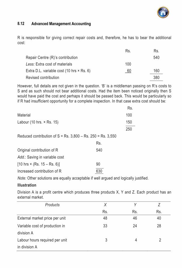
Advanced Management Accounting 8.12
R is responsible for giving correct repair costs and, therefore, he has to bear the additional cost:
Rs. Rs. Repair Centre (R)’s contribution 540 Less: Extra cost of materials 100 Extra D.L. variable cost (10 hrs × Rs. 6) 60 160 Revised contribution 380
However, full details are not given in the question. ‘B’ is a middleman passing on R’s costs to S and as such should not bear additional costs. Had the item been noticed originally then S would have paid the cost and perhaps it should be passed back. This would be particularly so if R had insufficient opportunity for a complete inspection. In that case extra cost should be:
Rs. Material 100 Labour (10 hrs. × Rs. 15) 150 250 Reduced contribution of S = Rs. 3,800 – Rs. 250 = Rs. 3,550
Rs. Original contribution of R 540 Add.: Saving in variable cost [10 hrs × (Rs. 15 – Rs. 6)] 90 Increased contribution of R 630 Note: Other solutions are equally acceptable if well argued and logically justified. Illustration Division A is a profit centre which produces three products X, Y and Z. Each product has an external market.
Products X Y Z Rs. Rs. Rs.
External market price per unit 48 46 40
Variable cost of production in 33 24 28 division A Labour hours required per unit 3 4 2 in division A

Transfer Pricing 8.13
Product Y can be transferred to Division B, but the maximum quantity that might be required for transfer is 300 units of Y.
The maximum external sales are:
X 800 units Y 500 units Z 300 units
Instead of receiving transfers of product Y from Division A, Division B could buy similar product in the open market at a sightly cheaper price of Rs. 45 per unit.
What should the transfer price be for each unit for 300 units of Y, if the total labour hours available in Division A are:
(a) 3,800 hours
(b) 5,600 hours
Solution Working Notes: (i) Hours required to meet maximum demand: External sales Hours reqd. Total Hrs.
per unit (i) (ii) (iii) = (i) × (ii) X 800 units 3 2,400 Y 500 units 4 2,000 Z 300 units 2 600 Total 5,000 (ii) Contribution per unit:
Product X Y Z Rs. Rs. Rs. Selling price 48 46 40
Less : Variable cost 33 24 28
Contribution per unit : (A) 15 22 12
Labour hours required per unit : (B) 3 4 2
Contribution per hour (Rs) : (A) / (B) 5 5.5 6
Ranking III II I

Advanced Management Accounting 8.14
(a) If only 3,800 hours are available in Division A. 300 units of Z (maximum), which will take* 600 hrs. 500 units of Y (maximum), which will take 2,000 hrs. 400 units of X to use remaining hrs. 1,200 hrs. 3,800 hrs. *Note : Labour hours required per unit are given in the question. If 300 units of Y are to be
transferred to ‘B’ division, then 1,200 hours will have to be used for production of Y instead of X. It means Division A will sacrifice production of 400 units of X, which are yielding Rs. 5 per hr. Given above is the optimum mix for Division A for 3,800 hrs. If 300 units of Y are to be transferred to ‘B’ division with time constraint of 3,800 hours, then additional 300 units of Y will have to be produced sacrificing the production of 400 units of X which is yielding contribution.
Transfer priceRs. (i) Variable cost of Y 24.00 Opportunity cost (ii) Contribution relating to ‘X’ forgone for
producing additional units of Y (4 hrs × Rs. 5*) 20.00
44.00 *Y takes 4 hours and in each hour production of X would have generated contribution of Rs. 5. (b) If 5,600 hours are available Maximum time required to meet external sales (Refer to Working note 1) 5,000 hrs.
Hours now available 5,600 hrs. (i) It means 600 hrs can be easily used for the production of Y and transfer price will be
variable cost only i.e. (600 hrs. ÷ 4 hrs) × Rs. 24 Rs. 3,600 Note: Y takes 4 hours per unit (ii) For producing additional 150 units,
production of X will be disturbed. Variable costs (i) 150 units of X @ Rs. 24 Rs. 3,600 Opportunity cost

Transfer Pricing 8.15
(ii) Contribution of ‘X’ units forgone (600 hrs. × Rs. 5) Rs. 3,000* 6,600Total price for 300 units 10,200∴Average transfer price should be Rs. 34 per unit *Contribution per hr. of X forgone.
Illustration Your company fixes the inter-divisional transfer prices for its products on the basis of cost, plus a return on investment in the division. The Budget for Division A for 1998-99 appears as under: Investment in Division A
Rs. Fixed Assets 5,00,000 Current Assets 3,00,000 Debtors 2,00,000 Annual fixed cost of the division 8,00,000 Variable cost per unit of product 10 Budgeted volume 4,00,000 units per year Desired ROI 28% Determine the transfer price for Division A. Solution The desired rate of return is 28% on investments. Investments include: (i) Fixed assets after depreciation (ii) Net working capital. In the question, current assets and debtors are given but current liabilities and creditors are not indicated. Therefore, these are assumed to have nil value. Investments
Rs. Fixed assets 5,00,000
Net working capital Rs. Current assets 3,00,000 Debtors 2,00,000 5,00,000
Total investments 10,00,000 The desired rate of return is 28%

Advanced Management Accounting 8.16
∴ The profit margin will be
28 .10,00,000
100Rs × Rs. 2,80,000
Budgeted volume 4,00,000 units Rs. Profit margin per unit (Rs. 2,80,000 ÷ 4,00,000 units) 0.70 Fixed cost per unit 2.00 (Rs. 2,80,000 ÷ 4,00,000 units) Variable cost per unit 10.00 Transfer price per unit 12.70 Ilustration A company is organised on decentralised lines, with each manufacturing division operating as a separate profit centre. Each division manager has full authority to decide on sale of the division’s output to outsiders and to other divisions. Division C has always purchased its requirements of a component from Division A. But when informed that Division A was increasing its selling price to Rs. 150, the manager of Division C decided to look at outside suppliers. Division C can buy the component from an outside supplier for Rs. 135. But Division A refuses to lower its price in view of its need to maintain its return on the investment. The top management has the following information : C’s annual purchase of the component 1,000 units A’s variable costs per unit Rs. 120 A’s fixed cost per unit Rs. 20 Required :
(i) Will the company as a whole benefit, if Division C bought the component at Rs. 135 from an outside supplier ?
(ii) If A did not produce the material for C, it could use the facilities for other activites resulting in a cash operating savings of Rs. 18,000. Should C then purchase from outside sources ?
(iii) Suppose there is no alternative use of A’s facilities and the market price per unit for the component drops by Rs. 20. Should C now buy from outside ?

Transfer Pricing 8.17
Solution (i) The company as a whole will not benefit if Division C bought the component from
an outside supplier at Rs. 135/- per unit Rs. Purchase cost from outside supplier 1,35,000 (1,000 units × Rs. 135 per unit) Less : Saving in variable cost of division 1,20,000 A by reducing Divisions’ output (1,000 units × Rs. 120 per unit) Net cost (benefit) to the company as a whole 15,000 The company as a whole will not benefit, as it will be required to incur an additional cost of Rs. 15,000 if Division C bought the company from outside supplier. (ii) The company will be benefitted if C purchased the component from an out-side
supplier and Division A uses the facilities for other activities. Rs. Rs. Purchase cost from outside supplier (1,000 units × Rs. 135) 1,35,000 Less : Savings in variable cost of Division A for the units purchased by Division C from outside (1,000 units × Rs. 120 per unit) 1,20,000 Cash operating saving of Division A for the use of facilities for other activities 18,000 1,38,000 Net cost (benefit) to the company as a whole (3,000) It is advisable that Division C should purchase the component from outside sources as this decision will benefit the company by Rs. 3,000. (iii) The company will be benefitted if C purchased the component from an out-side
supplier and there is no alternative use of Division A’s facilities. Purchase cost from outside supplier Rs. (1,000 units × Rs. 115) 1,15,000 Less : Saving in variable cost of Division A by reducing division’s output 1,20,000 (1,000 units × Rs. 120) Net cost (benefit) to the company (5,000) It is advisable that the Division C should buy the component from outside as this decision will benefit the company by Rs. 5,000.

Advanced Management Accounting 8.18
Illustration Division Z is a profit centre, which produces four products –A, B, C and D. Each product is sold in the external market also. Data for the period is as follows:
A B C DMarket price per unit Rs. 150 Rs.146 Rs.140 Rs.130Variable cost of production per unit Rs. 130 Rs.100 Rs. 90 Rs. 85Labour hours required per unit 3 4 2 3
Product D can be transferred to division Y, but the maximum quantity that might be required for transfer is 2,500 units of D. The maximum sales in the external market are : A 2,800 units B 2,500 units C 2,300 units D 1,600 units Division Y can purchase the same product at a slightly cheaper price of Rs.125 per unit instead of receiving transfers of product D from division Z. What should be transfer price for each unit for 2,500 units of D, if the total labour hours available in division Z are: (i) 20,000 hours? (ii) 30,000 hours? Solution Working note : Ranking of products when availability of time is the key factor
Product A B C D Rs. Rs. Rs. Rs.
Market price per unit 150 146 140 130 Less: Variable cost of production per unit 130 100 90 85Contribution per unit 20 46 50 45Contribution per hour 6.66 11.50 25 15
(Rs.20/3 hrs.) (Rs.46/4 hrs.) (Rs.50/2 hrs.) (Rs.45/3 hrs.) Ranking IV III I II
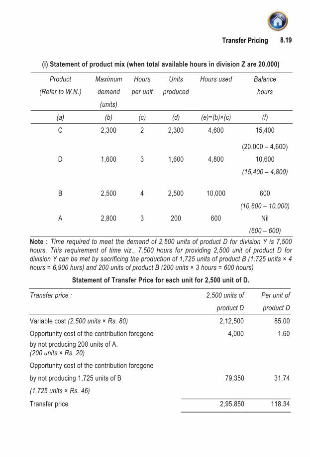
Transfer Pricing 8.19
(i) Statement of product mix (when total available hours in division Z are 20,000)
Product Maximum Hours Units Hours used Balance (Refer to W.N.) demand per unit produced hours
(units)
(a) (b) (c) (d) (e)=(b)×(c) (f)
C 2,300 2 2,300 4,600 15,400
(20,000 – 4,600) D 1,600 3 1,600 4,800 10,600 (15,400 – 4,800)
B 2,500 4 2,500 10,000 600 (10,600 – 10,000)
A 2,800 3 200 600 Nil (600 – 600)
Note : Time required to meet the demand of 2,500 units of product D for division Y is 7,500 hours. This requirement of time viz., 7,500 hours for providing 2,500 unit of product D for division Y can be met by sacrificing the production of 1,725 units of product B (1,725 units × 4 hours = 6,900 hurs) and 200 units of product B (200 units × 3 hours = 600 hours)
Statement of Transfer Price for each unit for 2,500 unit of D.
Transfer price : 2,500 units of Per unit of
product D product D
Variable cost (2,500 units × Rs. 80) 2,12,500 85.00Opportunity cost of the contribution foregone 4,000 1.60by not producing 200 units of A. (200 units × Rs. 20) Opportunity cost of the contribution foregone by not producing 1,725 units of B 79,350 31.74(1,725 units × Rs. 46)
Transfer price 2,95,850 118.34

Advanced Management Accounting 8.20
(ii) Statement of product mix (when total available hours in division Z are 30,000)
Product Maximum Hours Units Hours Balance
(Refer to W.N.) demand per unit produced used hours
(units)
(a) (b) (c) (d) (e)=(b)×(c) (f)
C 2,300 2 2,300 4,600 25,400
(30,000 – 4,600)
D 1,600 3 1,600 4,800 20,600
(25,400 – 4,800)
B 2,500 4 2,500 10,000 10,600
(20,600 – 10,000)
A 2,800 3 2,800 8,400 2,200
(10,600 – 8,400)
Note : The required time for producing 2,500 units of product D for divison Y is 7,500 hours. This requirement can be met to the extent of 2,200 hours out of the balance hours (as shown in the last column of the above table). The remaining re-quirement of 5,300 hours can be met by sacrificing the output of 1,766.66 units of product A. Statement of Transfer Price for each unit for 2,500 units of D
2,500 units of Per unit of product D product DVariable cost (2,500 units × Rs. 80) 2,12,500 85.00Opportunity cost of the contribution foregone by not producing 1,766.66 units of product A. 35,333.20 14.13(1,766.66 units × Rs. 20)
Transfer price 2,47,833.20 99.13
Illustration AB Ltd. manufactures foam, carpets and upholstery in the three divisions. Its oeprating state- ment for 1995-96 showing the performance of these divisions drawn for the use of management is reproduced below :

Transfer Pricing 8.21
(Rupees in ’000)
Sales revenue
Manufacturing Divisions Total 4,000
Foam Carpets Upholstery Sales revenue 1,600 (A) 1,200 1,200 4,000
Manufacturing Costs : Variable 1,200 700 680 2,580Fixed (Traceable) — 100 20 120
1,200 800 700 2,700
Gross Profit 400 400 500 1,300
Expenses : Administration 134 116 172 422Selling 202 210 232 644 336 326 404 1,066 (B)
Net Income 64 74 96Division’s Ranking 3rd 2nd Ist
(A) Sales include foam tansferred to the Upholstery division at its manufacturing cost of Rs. 2,00,000.
(B) Common expenses of Rs. 1,30,000 and Rs. 1,00,000 on account of administration and selling respectively stand apportioned to these divisions at 10% of Gross Profit in case of administration and 2.5% of Sales in case of selling expenses. Rest of Rs. 8,36,000 of the expenses are traceable to respective divisions.
The manager of the foam division is not satisfied with the above approach of presenting operating performance. In his opinion his division is best among all the divisions. He requests the management for preparation of revised operating statement using contribution approach and showing internal transfer at market price. You are required to : (a) Draw the revised operating statement using contribution approach and pricing the
internal transfer at market price. (b) Compute relevant ratios to show comparative profitability of these divisions and rank
them in the light of your answer at (a) above. Further, offer your comments on the contention of the manager of foam division.

Advanced Management Accounting 8.22
(c) State why the contribution approach and pricing of internal transfers at market price are more appropriate in realisitic assessment of the performance of various divisions.
Solution (a) Revised Operating Statement using Contribution approach
(Rs. ’000)
Divisions : Foam Carpets Upholstery Total Sales revenue 1,680 1,200 1,200 4,080(Refer to working note 1) Less : Variable manufacturing costs : 1,200 700 760 2,660(Refer to working note 2) Contribution : (A) 480 500 440 1,420Traceable Costs : Fixed manufacturing costs — 100 20 120Administration expenses 94 76 122 292(Refer to working note 3) Selling expenses 162 180 202 544(Refer to working note 4) Total : (B) 256 356 344 956
Net Contribution or Operating income : [(A) – (B)] 224 144 96 464Less : Common expenses (Rs. 130 + Rs. 100) 230Net income of the company 234Working Notes :
1. Computation of sales revenue of Foam division (Rs. ’000) Sales of foam division to outside customers 1,400 (Rs. 1,600 – Rs. 200) Less : Variable manufacturing costs 1,000 (Rs. 1200 – Rs. 200) Mark-up on outside sale 400

Transfer Pricing 8.23
Percentage of mark-up 40% (Rs. 400/Rs. 1000) × 100 Transfer price of foam to upholstery division 280 Sales of foam division to outside customers 1,400
Total 1,680 2. Computation of variable manufacturing costs of
Upholstery Division in (Rs. ’000) (Rs. 680 – Rs. 200 + Rs. 280) = Rs. 760
3. Computation of Traceable Administration Expenses
(Rs. ’000)
Divisions : Foam Carpets Upholstery Total
Given Administration expenses 134 116 172 422Less : Common expenses 40 40 50 130 (10% of Gross Profit) Traceable Administration expenses 94 76 122 292
4. Computation of Traceable Selling Expenses (Rs. ’000)
Divisions : Foam Carpets Upholstery TotalGiven Selling expenses 202 210 232 644Less : Common expenses 40 30 30 100 (2.5% of Sales) Traceable selling expenses 162 180 202 544
(b) Comparative Profitability & Ranking Statement (based on contribution approach relevant ratios calculated
by using figures of (a) part) (Rs. ’000)
Divisions : Foam Carpets Upholstery Contribution 28.57 41.67 36.67 margin ratio (in %) (Rs. 480/1680) × 100 (Rs. 500/1200) × 100 (Rs. 440/1200) × 100Ranking III I II Net Contribution 13.33 12 8

Advanced Management Accounting 8.24
ratio (in %) (Rs. 224/1680) × 100 (Rs. 144/1200) × 100 (Rs. 96/1200) × 100Or (Operating income ratio) Ranking I II III
Comment : The Manager of Foam Division, appears to be correct in raising objection over the approach used for presenting operating performance of three divisions for the year 1995–1996. His division is the best among all, on the basis of (Net Contribution/Sales) ratio which is the highest inspite of its contribution margin ratio to be the lowest. (c) The use of contribution approach for reporting is more realistic for assessing the perfor-
mance of various divisions as it considers variable and traceable costs only and avoids common costs while finding out profitability. This approach enables the management to rightly interpret the information. Further pricing of internal transfers at market price will give due credit to specific profit centre i.e. transferor.
Illustration City Instrument Company (CIC) consists of the Semi-conductor Division and the Mini-computer Division each of which operates as an indepedent profit centre. Semi-conductor Division em- ploys craftsmen, who produce two different electronic components, the new-high performance Super-chip and an older product called Okay-chip. These two products have the following cost characteristics :
Super-chip Okay chip
Material Parts Rs. 20 Parts Rs. 10
Labour 2 hours × Rs. 140 Rs. 280 1/2 hour × Rs. 140 Rs. 70
Annual Overhead in Semi-conductor Division is Rs. 40,00,000 all fixed. Owing to high skill level necessary for the craftsmen, the Semi-conductor Division’s capacity is set at 50,000 hours per year. To date, only one customer has developed a product utilising super-chip, and this customer orders a maximum of 15,000 super-chips per year at a price of Rs. 600 per chip. If CIC cannot meet his entire demand, the customer curtails his own production. The rest of the semi-conductor’s capacity is devoted to Okay-chips, for which there is unlimited demand at Rs. 120 per chip. The Mini-computer Division produces only one product, a process control unit, which requires a complex circuit board imported at a price of Rs. 600. The control unit’s costs are
Control Unit Material Circuit board Rs. 600 Other parts 80Labour 5 hours @ Rs. 100 500

Transfer Pricing 8.25
The Mini-Computer Division is composed of only a small assembly plant and all overhead is fixed at a total of Rs. 8,00,000 per year. The current market price for the control unit is Rs. 1,400 per unit. A joint research project has just revealed that with minor modifications, a single super-chip could be substituted for the circuit board currently used by the Mini-computer division. The modifica- tion would required an extra one hour of labour by Mini-computer’s staff, for a total of 6 hours per control unit. Mini-computer has therefore asked Semi-conductor division to declare a transfer price at which Semi-conductor division would sell super-chip internally. Required : (i) Mini-computer expects to sell 5,000 control units this year. From the overall view point of
CIC, how many super-chips should be transferred to Mini-computer Division to replace circuit boards ?
(ii) If the demand for the control unit is sure to be 5,000 units, but its price is uncertain, what should be the transfer price of super-chip to ensure proper decisions ? (All other data unchanged)
(iii) If demand for the control unit rises to 12,000 units at a price of Rs. 1,400 per unit, how many of 12,000 units should be built using Super-chip ? (All other data unchanged.)
Solution : Working Notes : 1. Contribution per hour of Super-chips and Okay-chips:
Super-chips Okay-chips Selling price per unit (Rs.) 600 120 Less : Variable cost per unit (Rs.) 300 80 Contribution per unit (Rs.) 300 40 Hours required per unit 2 0.5 Contribution per hour 150 (Rs. 300/2 hrs.) (Rs. 40/0.5 hrs.)
2 . Details of hours utilised in meeting the demand of 15,000 units of Super-chips and utilising the eremaining hours for Okay-chips out of available hours of 50,000 per annum:
Hours utilised for manufacturing 15,000 units of Super-chips 30,000 (15,000 units × 2 hours)
Hours utilised for manufacturing 40,000 units of Okay-chips 20,000 (40,000 units × 0.5 hours) 50,000

Advanced Management Accounting 8.26
3 . Contribution of a process control unit (using an imported complex circuit board) : Rs. Selling price per unit : (A) 1,400 Variable costs : Circuit board (Imported) 600 Other parts 80
Labour cost 500 (5 hours × Rs. 100) Total variable cost : (B) 1,180 Contribution per unit (Rs.) {(A) – (B)} 220 4 . Contribution of a process control unit (using a Super chip) : Rs. Selling price per unit : (A) 1,400 Variable costs : Super chip 300 (Material + Labour costs) Other parts 80
Labour cost 600 (6 hours × Rs. 100) Total variable cost : (B) 980 Contribution per unit : {(A) – (B)} 420 5 . Incremental contribution per unit of a process control unit, when instead of using
imported complex circuit board Super-chip is used : Incremental contribution per unit (Rs.) : 200 {Rs. 420 – Rs. 220} {Refer to working notes 3 & 4} (i) Super-chip to be trasferred to Mini Computer Division to replace Circuit Boards : Out of 50,000 available hours 30,000 hours are utilised for meeting the demand of
15,000 units of Super-chips, the rest 20,000 hours may be used for manufacturing 40,000 Okay-chips, which yields a contribution of Rs. 40 per unit for Rs. 80/- per hour (Refer to Working note 1) or a contribution of Rs. 160 per two-equivalent hours.
In case the company decides to forego the manufacturing of 20,000 units of Okay- chips in favour of 5,000 additional units of Super-chips to be used by Mini-Computer
Division (instead of complex imported Circuit Board) for manufacturing process control

Transfer Pricing 8.27
units. This decision would increase the existing contribution of Mini-Computer Division by Rs. 200/- per two-equivalent hours (Refer to Working note 5).
After taking into account the profit foregone of Okay-chips, the existing contribution of Mini-Computer Division of CIC would increase by Rs. 40 per two equivalent hours.
Hence the entire requirement of 5,000 units of Super-chips be produced and transferred to Mini-Computer Division.
(ii) Minimum transfer price of Super-chip to Mini Computer Division : = Variable cost of a Super-chip + Opportunity cost of foregoing the production
of an Okay-chip and using the craftman time for Super-chip
= Rs. 300 + 2 hours × Rs. 80 = Rs. 460 (iii) Super-chips to be produced for the production of 12,000 units of process con- trol
units : After meeting out the order of 15,000 Super-chips per year, the concern is left out with
20,000 hours. Use of Super-chips for control units production would increase the exist- ing contribution of Mini-Computer Division by Rs. 200/- per unit. Out of the remaining 20,000 craftmen hours, 10,000 units of Super-chips can be made, which may be used for the production of 10,000 process control units.
8.4 CONFLICT BETWEEN A DIVISION AND THE COMPANY Usually a conflict between a division of the company and the company as a whole is faced by the management of decentralised units when products or services are exchanged among different divisions of the company. Such a conflict becomes more significant in the case of those concerns where profitability is used as a criteria for evaluating the performance of each division. The essence of decentralisation is reflected in the freedom to make decisions. Under such a set up it is expected that the top management should not interfere with the decision making process of its subordinates heading different units. In other words, management of decentralised units is given autonomy with regard to decision making. The management of such companies also expects that each division should not only achieve its own objective necessary for evaluating the performance but should also achieve the objective of goal congruence. In case of failure of a division to achieve the objective of ‘goal congruence’ the management of the company may dictate their ‘transfer price’. Such interference of management of the company is usually the main basis of conflict between a division and the company as a whole. Further this conflict is aggravated if the management advocates the transfer of goods and services at cost. As such the transfer price will not reflect a good picture about the performance of the transferring division. The profitability of the transferring division will not be known by the use of such a transfer price.
Advanced Management Accounting 8.28
Each division appreciates the transfer of its goods/services at usual selling price/market price so as to arrive at the correct return/profitability figure, used for measuring the performance. There is no incentive to the transferring division if goods and services are transferred at variable cost. 8.5 MULTINATIONAL TRANSFER PRICING In the discussions above, we have focused on how transfer pricing policies affect the motivation of managers. However, in multinational companies, other factors may dominate. Multinational companies use transfer prices to minimize worldwide income taxes, import duties, and tariffs. For example, Nike might prefer to make its profits in a country, with its maximum corporate tax rate of 28%, rather than in some other place where the rate is 35%. Suppose a division in a high-income-tax-rate country produces a sub-assembly for another division in a low-income-tax-rate country. By setting a low transfer price, the company can recognize most of the profit from the production in the low-income-tax-rate country, thereby minimizing taxes. Likewise, items produced by divisions in a low-income-tax-rate country and transferred to a division in a high-income-tax-rate country should have a high transfer price to minimize taxes. Sometimes import duties offset income tax effects. Most countries base import duties on the price paid for an item, whether bought from an outside company or transferred from another division. Therefore, low transfer prices generally lead to low import duties. Consider a populated PCB maufactured by Alcatel Ltd. (Switzerland) with an 8% income tax rate and transferred to a division in India with a 40% income tax rare. In addition, suppose India imposes an import duty equal to 20% of the price of the item and that Alcatel cannot deduct this import duty for tax purposes. Suppose the full unit cost of a of populated PCB is Rs. 100, and the variable cost is Rs. 60. If tax authorities allow either variable- or full-cost transfer prices, which should Alcatel choose? By transferring at Rs. 100 rather than at Rs. 60, the company gain Rs. 4.80 per unit: Effect of Transferring at Rs. 100 instead of at Rs. 60 Income of the Swiss division is Rs. 40 higher;therefore it pays 8% x Rs. 40 more income taxes (Rs. 3.20)Income of the Indian division is Rs. 40 lower; therefore it pays 40% x Rs. 40 less income taxes (Rs.16.00) Import duty is paid by the India division on an additional Rs.100 – Rs.60 = Rs.40; there fore it pays 20% x Rs.40 more duty (Rs. 8) Net saving from transferring at Rs. 100 instead of Rs. 60 Rs. 4.80 Financial restricitions imposed by some governments may be avoided by an effective use of transfer price. For example, in case a country restricts the amount of dividend paid to foreign owners, it may be easier for a company to get cash from a foreign division in form of payments for poduct transferred rather than cash dividend. In summary, transfer pricing is more complex in a multinational company than it is in a domestic company. Multinational companies try to achieve more objectives through transfer- pricing policies, and some of the objectives can confil

Transfer Pricing 8.29
SELF-EXAMINATION QUESTIONS 1. What are the three general methods for determining transfer prices? 2. In transfer pricing, what is a common conflict between a division and the company as a
whole? 3. A company is organised on decentralised lines, with each manufacturing division
operating as a separate profit centre. Each divisional manager has full authority to decide on sale of the division’s output to outsiders and to other divisions.
Division C has always purchased its requirements of a component from Division A. But when informed that Division A was increasing its selling price to Rs. 150, the manager of Division C decided to look at outside suppliers.
Division C can buy the component from an outside supplier for Rs. 135. But Division Arefuses to lower its price in view of its need to maintain its return on the investment.
The top management has the following information : C’s annual purchase of the component 1,000 units A’s variable costs per unit Rs. 120 A’s fixed cost per unit Rs. 20 Required : (i) Will the company as a whole benefit, if Division C bought the component at Rs. 135 from
an outside supplier? (ii) If A did not produce the material for C, it could use the facilities for other activities
resulting in a cash operating savings of Rs. 18,000. Should C then purchase from outside sources?
(iii) Suppose there is no alternative use of A’s facilities and the marker price per unit for the component drops by Rs. 20. Should C now buy from outside?
4. Discuss briefly the concept of multinational transfer pricing? ANSWERS TO SELF-EXAMINATION QUESTIONS
3. (i) The company as a whole will not benefit, as it will be required to incur an additional cost of Rs. 10,000.
(ii) The Division C should purchase from outside as it will benefit the company by Rs. 3,000.
(iii) The Division C should buy the component from outside as this will benefit the company by Rs. 5,000.
9 Uniform Costing and Inter Firm Comparison
9.1 UNIFORM COSTING Meaning Uniform Costing is not a distinct method of costing. In fact, when several undertakings start using the same costing principles and/or practices they are said to be following uniform costing. The basic idea behind uniform costing is that the different concerns in an industry should adopt a common method of costing and apply uniformly the same principles and techniques for better cost comparison and common good. The principles and methods of compilation, analysis, apportionment and absorption of overheads differ from one concern to the other in the same industry; but if a common or uniform pattern is adopted by all, it helps mutually in cost control and cost reduction. Therefore, it is necessary that a uniform method of costing should be adopted by the member unit of an industry. 9.1.1 Objectives of Uniform Costing: The main objectives of Uniform Costing are as follows :— 1. Facilitates Comparison: To facilitate the comparison of costs and performances of
different units in the same industry; it provides objective basis. 2. Eliminates Unhealthy Competition: To eliminate unhealthy competition among the
different units of an industry. 3. Improves Efficiency: To improve production capacity level and labour efficiency by
comparing the production costs of different units with each other. 4. Provides Relevant Data: To provide relevant cost information/data to the Government for
fixing and regulating prices of the products. 5. Ensures Standardisation: To bring standardisation and uniformity in the operation of
participating units. 6. Reduces Cost: To reduce production, administration, selling and distribution costs, and to
exercise control on fixed costs.

Advanced Management Account 9.2
9.1.2 Essential requisites for the installation of Uniform Costing System : A successful system of uniform costing has the following requirements :— 1. The firms in the industry should be willing to share/furnish relevant data/information. 2. A spirit of cooperation and mutual trust should prevail among the participating firms. 3. Mutual exchange of ideas, methods used, special achievements made, research and
know how etc. should be frequent. 4. Bigger firms should take the lead towards sharing their experience and know-how with
the smaller firms to enable the latter to improve their performance. 5. Uniformity must be established with regard to several points before the introduction of
uniform costing in an industry. In fact, uniformity should be with regard to following points: (a) Size of the various units covered by uniform costing. (b) Production methods. (c) Accounting methods, principles and procedures used.
9.1.3 Advantages of Uniform Costing : The advantages accruing from the use of uniform costing system are as follows :- 1. The management of each firm will be saved from the exercise of developing and
introducing a costing system of its own. 2. A costing system devised by mutual consultation and after considering the difficulties and
circumstances prevailing in different firms is readily adopted and successfully implemented.
3. It facilitates comparison of cost figures of various firms to enable the firms to identify their weak and strong points besides controlling costs.
4. Optimum achievement of efficiency is attempted by all the firms by utilising the experience of other concerns in the industry.
5. Standing in the industry of each firm will be known by making a comparison of its cost data with others.
6. Services of cost consultants or experts may be available jointly to each firm in the industry by sharing their experiences and expenses.
7. Research and development benefits of bigger firms may be made available to smaller firms.
8. It helps in the reduction of labour turnover, as a uniform wage system is the pre-condition of a uniform costing system.
9. It helps Trade Associations in negotiating with the Government for any assistance or concession in the matters of taxation, exports, subsidies, duties and prices determination etc.

Uniform Costing and Inter Firm Comparison 9.3
10. Unhealthy competition is avoided among the firms in the same industry in framing pricing policies and submitting tenders.
11. Prices fixed on the basis of uniform costing are representative of the whole industry and thus are reliable.
12. Uniform costing provide a basis for the comparative assessment of the performance of two firms in the same industry but in different sectors.
13. It helps the Government in regulating the prices of essential commodities such as bread, sugar, cement, steel etc.
9.1.4 Limitations of Uniform Costing :
1. Sometimes it is not possible to adopt uniform standards, methods and procedures of costing in different firms due to differing circumstances in which they operate. Hence, the adoption of uniform costing becomes difficult in such firms.
2. Disclosure of cost information and other data is an essential requirement of a uniform costing system. Many firms do not wish to share such information with their competitors in the same industry.
3. Small firms in an industry believe that uniform costing system is only meant for big and medium size firms, because they cannot afford it.
4. It induces monopolistic trend in the business, due to which prices may be increased artificially and supplies withheld.
9.2 INTER-FIRM COMPARISON
Meaning
It is technique of evaluating the performance, efficiency, costs and profits of firms in an industry. It consists of voluntary exchange of information/data concerning costs, prices, profits, productivity and overall efficiency among firms engaged in similar type of operations for the purpose of bringing improvement in efficiency and indicating the weaknesses. Such a comparison will be possible where uniform costing is in operation.
An inter-firm comparison indicates the efficiency of production and selling, adequacy of profits, weak spots in the organisation, etc. and thus demands from the firm’s management an immediate suitable action. Inter-firm comparison may enable the management to challenge the standards which it has set for itself and to improve upon them in the light of the current information gathered from more efficient units. Such a comparison may be carried out in electrical industry, printing firms, cotton spinning firms, pharmaceuticals, cycle manufacturing, etc.

Advanced Management Account 9.4
9.2.1 Requisites of inter-firm comparison system : The following requisites should be considered while installing a system of inter-firm comparison :– 1. Centre for Inter-Comparison: For collection and analysing data received from member
units, for doing a comparative study and for dissemination of the results of study a Central body is necessary. The functions of such a body may be :– (a) Collection of data and information from its members; (b) Dissemination of results to its members; (c) Undertaking research and development for common and individual benefit of its
members; (d) Organising training programmes and publishing magazines.
2. Membership: Another requirement for the success of inter-firm comparison is that the firms of different sizes should become members of the Centre entrusted with the task of carrying out inter-firm comparison.
3. Nature of information to be collected: Although there is no limit to information, yet the following information useful to the management is in general collected by the Centre for inter-firm comparison. a. Information regarding costs and cost structures. b. Raw material consumption. c. Stock of raw material, wastage of materials, etc. d. Labour efficiency and labour utilisation. e. Machine utilisation and machine efficiency. f. Capital employed and Return on capital. g. Liquidity of the organisation. h. Reserve and appropriation of profit. i. Creditors and debtors. j. Methods of production and technical aspects.
4. Method of Collection and presentation of information: The Centre collects information at fixed intervals in a prescribed form from its members. Sometimes a questionnaire is sent to each member ; the replies of the questionnaire received by the Centre constitute the information/data. The information supplied by firms is generally in the form of ratios and not in absolute figures. The information collected as above is stored and presented to its members in the form of a report. Such reports are not made available to non-members.
9.2.2 Advantages of Inter-firm comparison : The main advantages of inter-firm comparison are :– 1. Such a comparison gives an overall view of the industry as a whole to its members– the
present position of the industry, progress made during the past and the future of the industry.

Uniform Costing and Inter Firm Comparison 9.5
2. It helps a concern in knowing its strengths or weaknesses in relation to others so that remedial measures may be taken.
3. It ensures an unbiased specialized reporting on particular problems of the concern. 4. It develops cost consciousness among members of the industry. 5. It helps Government in effecting price regulation. 6. It helps to improve the quality of products manufactured and to reduce the cost of
production. It is thus advantageous to the industry as well as to the society. 9.2.3 Limitations of inter-firm comparison The following are the limitations in the implementation of a scheme of inter-firm comparison : 1. Top management feels that secrecy will be lost. 2. Middle management is usually not convinced with the utility of such a comparison. 3. In the absence of a suitable Cost Accounting System, the figures supplied may not be
reliable for the purpose of comparison. 4. Suitable basis for comparison may not be available.
SUMMARY: • When several undertakings start using the same costing principles and/or practices
they are said to be following uniform costing. • The main objectives of Uniform Costing are as follows :
Facilitates Comparison Eliminates Unhealthy Competition Improves Efficiency Provides Relevant Data Ensures Standardisation Reduces Cost
• It is technique of evaluating the performance, efficiency, costs and profits of firms in an industry
An inter-firm comparison indicates the efficiency of production and selling, adequacy of proof- its, weak spots in the organisation, etc. and thus demands from the firm’s management an immediate suitable action
• Requisites of inter-firm comparison system are as follows: Centre for Inter-Comparison Membership Nature of information to be collected Method of Collection and presentation of information

Advanced Management Account 9.6
SELF-EXAMINATION QUESTIONS 1. Define Uniform costing. Explain its objectives. 2. What are the requisites for the installation of a Uniform Costing System? 3. What are the advantages of Uniform Costing ? State its limitations. 4. Enumerate the points on which uniformity is essential before introducing Uniform costing
system. 5. What to you mean by inter-firm comparison ? Give its advantages and limitations. 6. Describe the requisites to be considered while installing a system of inter-firm
comparison by an industry.

10 Cost Sheet, Profitability Analysis and Reporting
10.1 INTRODUCTION
A Cost Sheet or Cost Statement is “a document which provides for the assembly of the detailed
Cost of a Cost Centre or Cost Unit”. It is a detailed statement depicting the sub-division of cost arranged in a logical order under different heads.
The main advantages of a Cost Sheet are as follows :
1. It provides the total cost figure as well as cost per unit of production.
2. It helps in cost comparison.
3. It facilitates the preparation of cost estimates required for submitting tenders.
4. It provides sufficient help in arriving at the figure of selling price.
5. It facilitates cost control by disclosing operational efficiency.
10.2 COST SHEETS IN THE TRADITIONAL ERA OF COST AND MANAGEMENT ACCOUNTING
The traditional era of cost accounting can be divided into the following two phases;
• 1st half of the 20th century – Costs were classified as Direct Costs and Manufacturing overheads.
• 2nd half of the 20th century – Costs were classified as Direct Costs, Fixed overheads and Variable overheads.

Advanced Management Accounting 10.2
10.2.1 Debatable issues regarding the use of Cost Sheet during the 1st half of the 20th century Product Cost Sheets prepared during this era appeared to be as shown below:
Capacity : ———— units (in Rs.) Description Total cost Direct Cost Overheads Cost per unit per unit per unit
Bill of MaterialCost xxx xxx ———- xxx Direct Labour xxx xxx ———- xxx Manufacturing overheads xxx ———- xxx xxx Marketing and administrative xxx ———- xxx xxx Overheads Total cost per unit xxx Add desired profit xxx Desired selling price/unit xxx There are two issues of contention which immediately cross ones mind on looking at the cost sheet shown above. They are; 1. #What volume of activity should be used to project overheads so as to arrive at unit cost? 2. What should be the criteria to determine desired profit? #Possible answers to the volume of activity question, which needs to be addressed to determine the total unit cost, usually lean in the direction of expected volume, normal level of production or capacity of the plant. The answer to the second question is generally subjective. However, the use of ‘cost of capital’ concepts remains the most widespread. # In case one looks carefully at the Cost Sheet drawn above, it shall be clear that whose ever prepares the Cost Sheet has got enough information on the volume of activity to be conducted by the concerned company, because only if this information is available can one actually predict the amount of manufacturing overheads to be incurred in a future period. In a competitive market, one may safely argue, one can only know the volume of activity to be performed by having in his mind a tentative Market Price, strangely however, this is one of the primary objective of a Cost Sheet. Similarly the issue of desired profit, the calculation and computation of which is extremely subjective and hence contentious. 10.2.2 Cost Sheet prepared during the 2nd half of the 20th century As mentioned above, there are very subtle differences in the two types of cost sheets mentioned above. Unlike Cost Sheets of the 1st half the ones prepared during the latter period were characterised by the fixed and variable concepts. By doing so, they answered, to a certain extent, one of the contentious issues mentioned that is:

Cost Sheet, Profitability Analysis and Reporting 10.3
• Since variable cost of units is determined by engineering standards and other analytical techniques, they do away with the volume of activity question, which essentially then pertains to fixed costs. Product Cost Sheets prepared during this era appeared to be as shown below;
Capacity : ———— units (in Rs.) Description Total Cost Total Fixed Total Variable Fixed Cost Variable Cost Total Cost
Cost Cost per unit per unit per unit
Bill of Material xxx ———- xxx ———- xxx xxx Cost Direct Labour xxx ———- xxx ———- xxx xxx Manufacturing xxx xxx xxx xxx xxx xxx overheads Marketing and xxx xxx xxx xxx xxx xxx Administrative Overheads Total cost per unit xxx xxx xxx Add desired profit xxx Desired selling xxx price/unit 10.2.3 Activity Based Costing The contentious issue of volume of activity remained in this era although it then concerned only the fixed overheads. As pointed out above, the concept of imputing fixed cost per unit had its own shortcomings. To a large extent, such anomalies are done away with the use of Activity Based Costing (ABC). A Cost Sheet prepared with ABC concepts is shown below;
Cost Sheet (ABC) Variable costs Rs per Unit Direct materials Xx Direct labour Xx Variable manufacturing overhead Variable with number of units Xx Variable with product complexity(number of batches) Xx

Advanced Management Accounting 10.4
Variable with product diversity(number of products) Xx Variable marketing and administrative Xx Total variable cost per unit Xx Fixed cost Fixed manufacturing overhead Xx Fixed marketing and administrative Xx Total fixed cost per unit Xx Grand total cost per unit Xx Desired profit (mark up) Xx Target selling price per unit Xx A careful study of the differences in this era and the Activity Based Cost Sheet shows that ABC recognises two additional variable costs and is essentially designed to improve the accuracy of the total unit cost thereby impacting favourably the fixation of selling price. These two additional variable costs are as follows;
• Costs, which vary with product complexity, such as number of batches.
• Costs that vary with product diversity, such as number of products. Although, there are many critics of ABC who contend that the technique is nothing but an improvement over the traditional concepts, it is easy to see how ABC would be a better tool during times when customers become demanding in terms of ‘features’ of products because of which companies have to cater to slightly different types of production processes for essentially the same product. The Textile Machinery and Picture Tube industry in India faced such a situation during the mid 1990s when the government had allowed foreign companies to enter the Indian markets and the import duties on second hand goods, SKDs and CKDs were reduced drastically. Customers then had more choices; product diversity and complexity were the need of the hour. The benefits of ABC during such times are immense. 10.2.4 Market driven standard costs Unlike traditional costing concepts where a target selling price is established after computing the cost of a product, Target Cost Sheets use the selling price it believes the market will allow in order to determine the allowable cost. Hence, the allowable or target cost per unit is a market driven standard cost that has to be met if the desired profit are to be achieved. Cost per unit is computed as follows:
Target Cost Sheet (Rs per unit) Selling price (prevailing in a competitive setting) Xx Less desired profit Xx Target or allowable cost Xx

Cost Sheet, Profitability Analysis and Reporting 10.5
Hence in Target Costing what counts is the need to produce at an allowable cost. This idea may mean that now the distinction between fixed and variable components is immaterial. It also implies that in case one intends to continuously improve, this allowable target cost should be reduced over time. Such reductions shall need an empowered workforce because it is the one, which is nearest to the action and so in the best position to lead towards a path of continuous improvement. 10.3 PROFITABILITY STATEMENTS 10.3.1 Direct product profitability (DPP) : As traditional absorption costing, which normally uses labour hours as a basis for absorption, is rarely suitable for service and retail organizations other methods had to be devised. One relatively new way of spreading overheads in retail organisations, which is used in the grocery trade in particular, is direct product profitability (DPP). DPP started in the USA in the 1960s at General Electric, and was then taken up and used by Proctor and Gamble in the 1980s. In 1985 the Food Marketing Institute in the USA laid down a standard approach to the system and two years later DPP was taken up by the Institute of Grocery Distribution in the U.K. The system described below was introduced in the late 1980s and has since undergone transformation as activity based costing. In recent years DPP has developed considerably in parallel with activity-based costing. DPP has become much more sophisticated and is now very similar to activity-based costing. One of the reasons for its development during the 1990s has been the development of EPOS and EFTPOS (electronic point of sale and electronic funds transfer) systems that have enabled access to the detailed data needed for direct product cost and profitability calculations. Even in 1993 Doherty et al said that : “DPP in retailing is not and cannot be fully-fledged costing system, where every last penny of expense has to be recovered. The level of cost information available to retailers is generally not detailed enough to allow for that.” Since then technology has improved and it is quite possible to cost product lines with reasonable accuracy. Benefits of DPP • Better cost analysis
• Better pricing decisions
• Better management of stores and warehouse space The rationalisation of product ranges. Direct product profitability statement : Retail organisations traditionally deducted the boughtin cost of goods from the selling price to give a gross margin. The gross margin is useless measure for controlling the costs of the organisation itself or making decisions about the profitability of the different products. This is because none of the costs generated by the retail organisation itself are included in its calculation. For example, it does not include the storage costs of the different goods and these costs vary considerably from one good to another. A method was needed which related the indirect costs to the goods according to the

Advanced Management Accounting 10.6
way the goods used or created these costs. Indirect costs, for DPP may be analysed into basic cost categories as follows : (i) Overhead cost : This is incurred through an activity that is not directly linked to a
particular product. (ii) Volume related cost : The cost is incurred in relation to the space occupied by products.
This includes storage and transport costs. (iii) Product batch cost : This cost is often a time based cost. If product items (that is a
number of identical products which are handled together as a batch) are stocked on shelves a labour time cost is incurred.
(iv) Inventory financing costs : This is the cost of tying up money in stock and is the cost of the product multiplied by interest rate per day or per weak.
Table 1, given below shows the DPP for good A. Directly attributable costs have been grouped into three categories and are deducted from the gross margin to determine the good’s DPP.
Table 1. Direct product profit for good A
Rs Rs.
Selling price p.u. 1.50 Less : Bought-in price 0.80 Gross margin 0.70 Less : Direct product costs : Warehouse costs 0.16 Transport costs 0.18 Store costs 0.22 0.56 Direct product profit p.u. 0.14 Warehouse and store costs will include items such as labour, space and insurance costs, while transport costs will include labour, fuel and vehicle maintenance costs. The usual way to spread these costs across the different goods sold is in relation to volume or area occupied, as most costs increase in direct proportion to the volume of the good or the space it occupies. However, there are some exceptions to this; for example, insurance costs may be better spread on value or on a risk index. Risk is greater with refrigerated or perishable goods. Refrigeration costs must only be related to those products that need to be stored in the refrigerator.
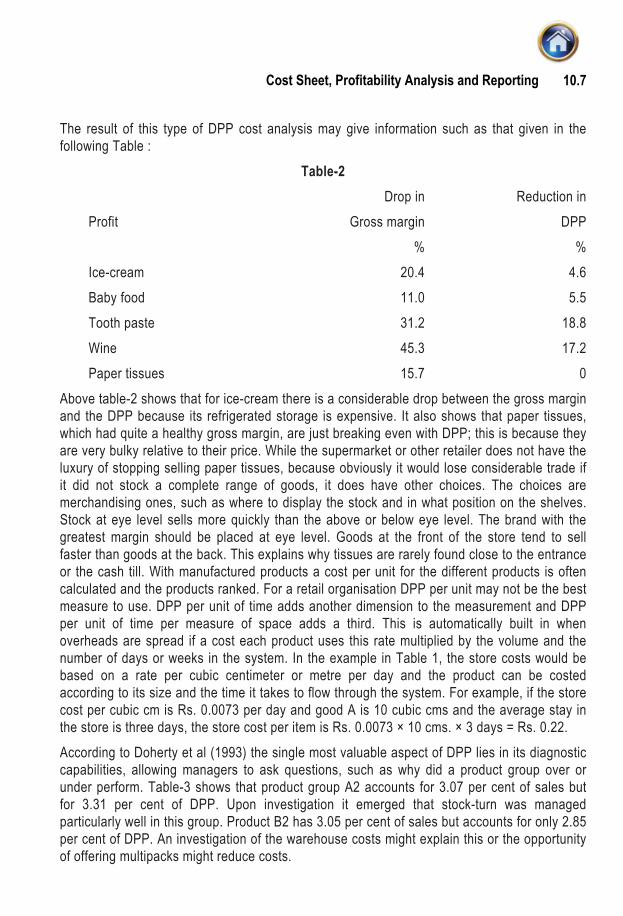
Cost Sheet, Profitability Analysis and Reporting 10.7
The result of this type of DPP cost analysis may give information such as that given in the following Table :
Table-2 Drop in Reduction in Profit Gross margin DPP % % Ice-cream 20.4 4.6 Baby food 11.0 5.5 Tooth paste 31.2 18.8 Wine 45.3 17.2 Paper tissues 15.7 0
Above table-2 shows that for ice-cream there is a considerable drop between the gross margin and the DPP because its refrigerated storage is expensive. It also shows that paper tissues, which had quite a healthy gross margin, are just breaking even with DPP; this is because they are very bulky relative to their price. While the supermarket or other retailer does not have the luxury of stopping selling paper tissues, because obviously it would lose considerable trade if it did not stock a complete range of goods, it does have other choices. The choices are merchandising ones, such as where to display the stock and in what position on the shelves. Stock at eye level sells more quickly than the above or below eye level. The brand with the greatest margin should be placed at eye level. Goods at the front of the store tend to sell faster than goods at the back. This explains why tissues are rarely found close to the entrance or the cash till. With manufactured products a cost per unit for the different products is often calculated and the products ranked. For a retail organisation DPP per unit may not be the best measure to use. DPP per unit of time adds another dimension to the measurement and DPP per unit of time per measure of space adds a third. This is automatically built in when overheads are spread if a cost each product uses this rate multiplied by the volume and the number of days or weeks in the system. In the example in Table 1, the store costs would be based on a rate per cubic centimeter or metre per day and the product can be costed according to its size and the time it takes to flow through the system. For example, if the store cost per cubic cm is Rs. 0.0073 per day and good A is 10 cubic cms and the average stay in the store is three days, the store cost per item is Rs. 0.0073 × 10 cms. × 3 days = Rs. 0.22. According to Doherty et al (1993) the single most valuable aspect of DPP lies in its diagnostic capabilities, allowing managers to ask questions, such as why did a product group over or under perform. Table-3 shows that product group A2 accounts for 3.07 per cent of sales but for 3.31 per cent of DPP. Upon investigation it emerged that stock-turn was managed particularly well in this group. Product B2 has 3.05 per cent of sales but accounts for only 2.85 per cent of DPP. An investigation of the warehouse costs might explain this or the opportunity of offering multipacks might reduce costs.

Advanced Management Accounting 10.8
Table–3 DPP values by Product Group. From Doherty et al 1993.
Product Sales as a % DPP as a %
Group of total sales of total DPP
A1 3.20 3.40
A2 3.07 3.31
B1 2.84 2.89
B2 3.05 2.85
C1 2.75 2.66
A3 2.26 2.48
10.3.2 Customer profitability analysis : In many organisations it is just as important to cost customers as it is to cost products. Different customers or groups of customers differ in their profitability. This is a relatively new technique that ABC makes possible because it creates cost pools for activities. Customers use some activities but not all, and different groups of customers have different ‘activity profiles’. Service organisations, such as a bank or a hotel, in particular need to cost customers. A bank’s activities for a customer will include the following types of activities :
• Withdrawal of cash
• Unauthorised overdraft
• Request for a statement
• Stopping a cheque
• Returning a cheque because of insufficient funds. Different customers or categories of customers will each use different amounts of these activities and so customer profitability profiles can be built up, and customers can be charged according to the cost to serve them. A hotel may have activities that are provided for specific types of customers, such as well laid-out gardens, a swimming pool and a bar. Older guests may appreciate and use the garden, families use the swimming pool and business guests use the bar. If the activities are charged to the relevant guests a correct cost per bed occupied can be calculated for this type of category. This will show the relative profitability and lead to strategies for encouraging the more profitable guests. Even a manufacturing organisation can benefit from costing its customers. Not all customers cost the same to serve even if they require the same products. Some customers may be located a long way from the factory and transport may cost more. Other customers may be disruptive and place rush orders that interrupt production scheduling and require immediate, special transport. Some customers need after sales service and help with technical matters, etc.

Cost Sheet, Profitability Analysis and Reporting 10.9
Illustration : A manufacturing organisation has four different customers A, B, C and D. A single product is sold to them at different prices because of trade discount offered. Data is give for cost per unit of business activity. You are required to prepare customer profitability statement.
Information on four customers
Customers A B C D
No. of units sold 60,000 80,000 1,00,000 70,000
Selling price net of discount 25p 23p 21p 22p
No. of sales visits 2 4 6 3
No. of purchase orders 30 20 40 20
No. of deliveries 10 15 25 14
Kilometres per journey 20 30 10 50
No. of rush deliveries — — 1 2
Cost of each activity
Sales visit Rs. 210 per visit
Order placing Rs. 60 per order
Product handling Rs. 0.10 per item
Normal delivery cost Rs. 2 per kilometre
Rushed delivery cost Rs. 200 per delivery
Customer profitability Statement
Customers A B C D
Rs. Rs. Rs Rs.
Revenue net of discount 15,000 18,400 21,000 15,400
(60,000 × Rs. 0.25) (80,000 units × 0.23) (1,00,000 × 0.21) (70,000 × 0.22)
Costs :
Sales visits 420 840 1,260 630
Ordering processing 1,800 1,200 2,400 1,200
Product handling 6,000 8,000 10,000 7,000
Normal Delivery 400 900 500 1,400

Advanced Management Accounting 10.10
Rush deliveries — — 200 400
8,620 10,940 14,360 10,630
Operating profit 6,380 7,460 6,640 4,770
Percentage profitability 43% 41% 32% 31%
It is apparent from above solution that all four customers are profitable, but customers C and D not particularly so when compared with customers A and B. There are several reasons for this range in profitability one reason is the negotiation of favourable terms such as higher trade discount as compared to other customers.
Benefits of customer profitability analysis.
1. It helps the supplier to identify which customers are eroding overall profitability and which customers are contributing to it.
2. It can help to provide a basis for constructive dialogue between buyer and seller to improve margins.
10.4 THE BALANCED SCORECARD
The Balanced Scorecard can be defined as ‘an approach to the provision of information to management to assist strategic policy formulation and achievement’. It emphasizes the need to provide the user with a set of information, which addresses all relevant areas of performance in an objective and unbiased fashion. The information provided may include both financial and non financial elements, and cover areas such as profitability, customer satisfaction, internal efficiency and innovation’. It shall be clear from the above definition that the central idea of the Balanced Scorecard is that managers should develop the measures on which they manage the business from four different perspectives:
1. customer satisfaction
2. internal business process e.g., operating cycle time.
3. kaizen approach (can we continue to improve and create value)
4. financial e.g., operating income by segments.

Cost Sheet, Profitability Analysis and Reporting 10.11
The following figure summarises the ideas of a Balanced Scorecard:
FINANCIALPERSPECTIVE
To succeed financially howshould a company appearto its stakeholderse.g. Quaterly sales growth,
CUSTOMERPERSPECTIVE
To achieve its vision how should a company appear to its shareholders e.g. I n f or m at io n on new products, their % age sales, On time delivery,
INTERNAL BUSINESSPERSPECTIVE
To satisfy its shareholders and c us tom ers wha t business process should a c om pan y ado pt e .g . Technology capability.
VISION &STRATEGY
INNOVATION &LEARNING
PERSPECTIVE
To achieve its vision how should a company sustain its ability to change and innovate e.g. Technology leadership, Product focus etc
The ultimate result of using the Balanced Scorecard approach should be an improved longterm financial performance. Since the scorecard gives equal importance to the relevant non – financial measures, it should discourage the short termism that leads to cuts in spending on new product development, human resource development etc which are ultimately detrimental for the future prospects of the company. The responsibility to devise and implement a Balanced Scorecard should be that of the managers working with the business. Since every company is different, it shall need to work out for itself the various financial and non – financial measures, which need to be focussed upon for its own development. Since the Balanced Scorecard is recommended as a management tool used both for internal and external reporting purposes, it is again the manager’s responsibility to decide as to what information needs to be disclosed and how any problems of confidentiality can best be overcome.

Advanced Management Accounting 10.12
The following are some reasons why Balanced Scorecards sometimes fail to provide for the desired results;
• Managers mistakenly think that since they already use non – financial measures, they already have a Balanced Scorecard.
• Senior executives misguidedly delegate the responsibility of the Scorecard implementation to middle level managers.
• Company’s try to copy measures and strategies used by the best companies rather than developing their own measures suited for the environment under which they function.
• There are times when Balanced Scorecards are thought to be meant for reporting purposes only. This notion does not allow a Business to use the Scorecard to manage Business in a new and more effective way.
It may be noted that the above-mentioned difficulties refer to the internal use of the Scorecard, unless it is used internally successfully, it should not be used as a basis for external reporting.
SELF- EXAMINATION QUESTIONS 1. How is a conventional Cost Sheet different from Cost Sheets prepared for ABC and
Target Costing purposes. Disucss 2. Briefly explain the meaning of Direct Product Profitability Statement and Customer
Profitability Statement. 3. Explain the Procedure of work-in-progress inventory under job order costing method.

11Linear Programming
LEARNING OBJECTIVES :
After studying this unit you will be able to :
� Formulate a problem in LP
� Understand the circumstances in which LP technique can be used
� Calculate marginal rates of substitution and opportunity cost using the graphic method
� Construct the initial tableau using the Simplex Method
� Explain the meaning odf entries in each column of final tableau
� Describe hoe technique of Linear Programming can be used in decision making,planning and control
11.1 INTRODUCTION
Linear programming is a mathematical technique for determining the optimal allocation of re-sources and achieving the specified objective when there are alternative uses of the resourceslike money, manpower, materials, machines and other facilities. The objective in resource allo-cation may be either cost minimization or profit maximization. The technique of linear program-ming is applicable to all problems in which the total effectiveness about the use of resources canbe expressed as a linear function of individual allocations, and the limitations on resources giverise to linear equalities or inequalities of individual allocations. The adjective linear, is to beparticularly noted here. It implies that all the limitations or constraints and the objective must beexpressed as linear functions.
Although the technique of linear programming is applicable to all such problems, there are somemore easy methods for solving specific categories of problems. Special algorithms have beenevolved to ease up computational task. The algorithms have acquired special names of theirown. This has led to the following categories of the linear programming problems :
(i) General Linear Programming Problems.
(ii) Transportation Problems.
(iii) Assignment Problems.

11.2 Advanced Management Accounting
We know that there is an opportunity cost for scarce resources that should be included in therelevant cost calculation for decision making and variance calculations. In practice severalresources may be scarce. The opportunity cost of these scarce resources can be determined bythe use of linear programming techniques. Our objective in this chapter is to examine linearprogramming techniques and to consider how they can be applied to some specific types ofdecisions that a firm may have to make.
11.1.1 General Linear Programming Problems :An examination of the following simple exampleshould illustrate the basic concepts of linear programming problem (abbreviated as LPP).
Illustration
A small scale industry unit manufactures two products, X1 and X
2 which are processed in the
machine shop and the assembly shop. The time (in hours) required for each product in theshops are given in the matrix below. Profit per unit is also given along.
Machine shop Assembly shop Profit per unit
Product X1
2 hours 4 hours Rs. 3
Product X2 3 hours 2 hours Rs. 4
Total time available (hours) 16 16
(in a day)
Assuring that there is unlimited demand for both products how many units of each should beproduced every day to maximize total profit ?
Let x1 and x2 be the number of units of X1 and X2 respectively that maximize the profit.
To begin solving the problem, let us restate the information in mathematical form. To do so, weintroduce a term "objective function". This refers to the expression which shows the relationshipof output to profit.
3x1 = total daily profit from the sale of x1 units product X1
4x2 = total daily profit from the sale of x
2 units product X
2
Objective function Max Profit = 3x1 + 4x2
Department time constraints
Time used in making x1 and x
2 units of two products must not exceed the total daily time
available in two shops. In other words, (the hours required to make 1 unit of product X1)multiplied by (the number of units of product X
1) plus ( the hours required to make 1 unit of
product X2) multiplied by (the number of units of product X2) must be less than or equal tothe daily time available in each shop. Mathematically it is stated as
2x1 + 3x
2 ≤ 16 Machine shop constraint
4x1 + 2x2 ≤ 16 Assembles shop constraint
In order to obtain meaningful answers, the values calculated for x1 and x2 cannot be negatives;they must represent real product X1 and product X2. Thus, all elements of the solution to theformulated linear programming problem must be either greater than or equal to 0 (x1 > 0, x2 > 0).The machine and assembly shops contraints are called structural constraints.

11.3Linear Programming
The problem can be summarized in a mathematical form as below :
Maximize:
Profit = 3x1 + 4 x
2
Subject to the constraints
2x1 + 3 x2 ≤ 16
4x1 + 2x
2 ≤ 16
x1 ≥ 0, x
2 > 0.
M ethod of L inear Program m ing
G raphica l M ethod S im plex M ethod
11.2 GRAPHICAL METHOD
The graphical method discussed here provides necessary grounding in understanding thecomputational steps of the simplex algorithms, it itself being of little use in handling practicalproblems. It is possible to solve conveniently linear programming problems graphically as longas the number of variables (products, for example) are not more than two. Before we proceed toexplain the graphical method, let us first know how linear inequalities are handled graphically.
11.2.1 Linear inequalities in one variable and the solution space
Any relation or function of degree one that involves an inequality sign is a linear inequality. It maybe of one variable, or, may be of more than one variable. Simple examples of linear inequalitiesare those of one variable only; viz. x > 0, x < 0, etc.
x > 0 x < 0
-3 -2 -1 0 1 2 3 -3 -2 -1 0 1 2 3
The values of the variables that satisfy an inequality are called the solution space, and is abbre-viated as S.S. The solution spaces for (i) x > 0, (ii) x < 0 are shown by the dark portion in theabove diagrams.
11.2.2 Linear inequalities in two variables : Now we turn to linear inequalities in two variablesx, and y, and shade a few S.S.
x>0 x ≥ 0x>0y >0
x ≥ 0y ≥ 0
x
yyy
xx
y
x

11.4 Advanced Management Accounting
Note : The pair of inequalities x ³ 0, y ³ 0 playan important role in linear programmingproblems.
Let us now consider a linear inequality in twovariables given by
3x + y < 6.
The inequality mentioned above is true for certainpairs of numbers, (x, y) that satisfy 3x + y < 6. Bytrial, we may arbitrarily find such a pair to be (1,1)because 3 × 1 + 1 = 4, and 4< 6.
Linear inequalities in two variables may be solvedeasily by extending our knowledge of straight lines.
For this purpose, we replace the inequality by anequality and seek the pairs of number that satisfy 3x + y = 6. We may write 3x + y = 6 as y = 6– 3x, and draw the graph of this linear function.
Let x = 0 so that y = 6. Let y = 0, so that x = 2
Any pair of numbers (x,y) that satisfies the equation y = 6 – 3x falls on the line AB.
Therefore, if y is to be less than 6 – 3x for thesame value of x, it must assume a value that isless than the ordinate of length 6 – 3x.
All such points (x,y) for which the ordinate isless than 6 – 3x lie below the line AB.
The region where these points fall is indicated byan arrow and is shaded too in the diagram above.
Now we consider two inequalities
3x + y < 6 and x – y < – 2
being satisfied simultaneously by x and y.
The pairs of numbers (x, y) that satisfy both theinequalities may be found by drawing the graphsof the two lines y = 6 – 3x and y = 2 + x, anddetermining the region where both the inequalities hold. It is convenient to express each equalitywith y on the left-side and the remaining terms in the right-side.
The first inequality 3x + y < 6 is equivalent to
y < 6 – 3x
and requires the value of y for each x to be less than that of y = 6 – 3x. This inequality istherefore satisfied by all points lying below the line y = 6 – 3x. The region where these points fallhas been shaded in the previous diagram.
x0
B
(2, 0)
Figure 2
6 - 3 x
yA
(0, 6)
(x, y)
A
0
y
X
B

11.5Linear Programming
y
x
yA
C
BD
yy = + 2 x
x(0 ,2 )
(-2 ,0 )
0
We consider the second inequality x – y < – 2, and note that this is equivalent to y > 2 + x.
It requires the value of y for each x to be larger than that of y = 2 + x. This inequality is, therefore,satisfied by all points lying above the line y = 2 + x.
The region is indicated by an arrow on the line y = 2 + x
For x = 0, y = 2 + 0 = 2. For y = 0, 0 = 2 + x \ x = – 2.
By superimposing the above two graphs we determine the common region ACD in which thepairs (x,y) satisfy both the inequalities.
Note : [1] The inequalities 3x + y < 6 and x - y < 2 differ from the preceding ones in that these alsoinclude equality signs. It means that the points lying on the corresponding lines are also includedin the region.
[2] The procedure may be extended to any number of inequalities.
11.2.3 Graphical solution for linear programming problem : We consider the problem ofmaximizing a linear function Z = x + 2 y subject to the restrictions
x > 0, y > 0, x < 6, y < 7, x + y < 12

11.6 Advanced Management Accounting
We note that the above inequalities may be grouped as follows:
⎭⎬⎫
⎩⎨⎧
≤≥
6
0
x
x
⎭⎬⎫
⎩⎨⎧
≤≥
7
0
y
y, x+ y ≤ ⋅12
y
��
9=x
X
y
�
y ≥ 0, y ≤ 7x ≥ 0, x ≤ 6
y
XO
x +y =
12
x + y ≤ 12
y = 7

11.7Linear Programming
By superimposing the above three diagrams, we determine the common region in the xy planewhere all the five inequalities are simultaneously satisfied.
This common region is known as feasible region or the solution set (or the polygonal convexsets).
A region is said to be bounded if it can be totally included within a (very large) circle. The shadedregion enclosed by deep lines in the previous diagram is bounded, since it can be includedwithin a circle.
Corresponding to an arbitrary definite value for Z, Z = x + 2y becomes an equation of a straightline. Let Z =2, 4, etc.
For Z = 2, we have x + 2 y = 2.
Let x = 0, so that y = 1.
Let y = 0, so that x = 2.
Next, let us suppose Z = 4.
In this case Z = x+2y takes the form x + 2 y = 4.
Let x = 0, so that y = 2.
Let y = 0, so that x = 4.
On drawing the graphs for both the abovelines we observe that each one of them in-tersects the feasible region. Here we arekeen to determine a point in the feasibleregion which makes Z maximum (i.e., aslarge as possible) we would prefer any pointin the feasible region that lies on x+ 2y =4over any point that lies on x + 2 y =2.
y
0
Z=0Z=2Z=4 Z = 7
Z = 1 9
X
x
(0 ,7 )
0 (6 ,0 )
(6 ,6 )
(0 ,0 )
y

11.8 Advanced Management Accounting
Following the same reasoning we find that we can get point in the feasible region for
which Z is maximum. The maximum value for Z is achieved when the line x + 2 y = Z is movedparallel to itself upward as far as possible subject to the restriction that it must intersect thefeasible region (shown by the deep line in the diagram on previous page). This is seen to occurwhen it passes through the point (5,7) the point of intersection of x + y = 12 and y = 5. It is notedthat this point (5,7) is one of the corner points (or extreme points) of the solution set.
We may similarly find the point in the feasible region for which Z is minimum. It is found to occurat (0,0) which is again a corner point of the solution set but situated opposite to the point forwhich Z is maximum. The values of x and y so determined constitutes the solution to theproblem.
Thus the objective function attains a maximum or a minimum value at one of the cornerpoints of the feasible solution known as extreme points of the solution set. Once theseextreme points (the points of intersection of lines bounding the region) are known, a compact matrixrepresentation of these points is possible. We shall denote the matrix of the extreme points by E.
The coefficients of the objective function may also be represented by a column vector. We shallrepresent this column vector by C.
The elements in the product matrix EC shows different values, which the objective functionattains at the various extreme points. The largest and the smallest elements in matrix EC arerespectively the maximum and the minimum values of the objective function. The row in matrixEC in which this happens is noted and the elements in that row indicate the appropriate pairingand is known as the optimal solution.
In the context of the problem under consideration.
x y
E =
⎟⎟⎟⎟⎟⎟
⎠
⎞
⎜⎜⎜⎜⎜⎜
⎝
⎛
66
06
75
70
00
, C = ⎥⎦
⎤⎢⎣
⎡2
1
EC =
⎟⎟⎟⎟⎟⎟
⎠
⎞
⎜⎜⎜⎜⎜⎜
⎝
⎛
66
06
75
70
00
⎥⎦
⎤⎢⎣
⎡2
1 =
⎟⎟⎟⎟⎟⎟
⎠
⎞
⎜⎜⎜⎜⎜⎜
⎝
⎛
×+××+××+××+××+×
2616
2016
2715
2710
2010
=
⎟⎟⎟⎟⎟⎟
⎠
⎞
⎜⎜⎜⎜⎜⎜
⎝
⎛
18
6
19
14
0
The given objective function viz. Z = x + 2y is maximum at the points (5, 7) present in the third rowof the matrix E. Thus the optimal solution is x = 5, y = 7, and the maximum value of the objectivefunction is 19.
x
y
x
y

11.9Linear Programming
We now list the steps to be followed under graphical solution to a linear programming problem.
Step1. Determine the region that satisfies the set of given inequalities.
Step 2. Ensure that the region is bounded*. If the region is not bounded, either there areadditional hidden conditions which can be used to bound the region or there is nosolution to the problem.
Step 3. Construct the matrix E of the extreme points, and the column vector C of the objectivefunction.
Step 4. Find the matrix product EC. For maximization, determine the row in EC where thelargest element appears; while for minimization, determine the row in EC where thesmallest element appears.
Step 5. The objective function is optimized corresponding to the same row elements of theextreme point matrix E.
Note : If the slope of the objective function be same as that of one side of feasible region,there are multiple solutions to the problem. However, the optimized value of theobjective function remains the same.
11.2.4 Application of Graphical Method
Illustration
A manufacturer produces two products A and B, and has his machines in operation for 24 hoursa day. Production of A requires 2 hours of processing in machine M1 and 6 hours in machine M2.Production of B requires 6 hours of processing in machine M1 and 2 hours in machine M2. Themanufacturer earns a profit of Rs. 5 on each unit of A and Rs. 2 on each unit of B. How manyunits of each product should be produced in a day in order to achieve maximum profit?
Solution
Let x1 be the number of units of type A product to be produced, and x2 is that of type B product tobe produced. The formulation of the L.P.P. in this case is as below :
Maximize Z = 5x1 + 2x2
subject to the constraints.
x1 ≥ 0, x2 ≥ 0,
2x1 + 6x2 ≤ 24,
6x1 + 2x2 ≤ 24.
For the line 2x1 + 6x
2= 24,
let x1 = 0, so that x2 = 4;
let x2 = 0, so that x1 = 12;
* It is inconceivable for a practical problem to have an unbounded solution.
x 1
x 2
(12,0)E1 (0,0)
E4 (4,0)
E3 (3,3)
(0,12)
6x1 +2x
2 =24 2x1+6x2=24E2 (0,4 )

11.10 Advanced Management Accounting
For the line 6x1 + 2x2 = 24;
let x1 = 0, so that x
2 = 12;
let x2 = 0, so that x
1 = 4.
The shaded portion in the diagram is the feasible region and the matrix of the extreme points E1,E2, E3 and E4 is
x1 x2
E =
4
3
2
1
E
E
E
E
0
3
4
0
4
3
0
0
⎟⎟⎟⎟⎟
⎠
⎞
⎜⎜⎜⎜⎜
⎝
⎛
The column vector for the objective function is C = 2
1
2
5
x
x⎥⎦
⎤⎢⎣
⎡
The column vector the values of the objective function is given by
EC = ⎟⎟⎟⎟⎟
⎠
⎞
⎜⎜⎜⎜⎜
⎝
⎛
04
33
40
00
⎥⎦
⎤⎢⎣
⎡2
5 =
⎟⎟⎟⎟⎟
⎠
⎞
⎜⎜⎜⎜⎜
⎝
⎛
×+××+××+××+×
2054
2353
2450
2050
=
4
3
2
1
E
E
E
E
20
21
8
0
⎟⎟⎟⎟⎟
⎠
⎞
⎜⎜⎜⎜⎜
⎝
⎛
Since 21 is the largest element in matrix EC, therefore the maximum value is reached at theextreme point E3 whose coordinates are (3,3).
Thus, to achieve maximum profit the manufacturer should produce 3 units each of both theproducts A and B.
Illustration
A company produces two types of presentation goods A and B that require gold and silver. Eachunit of type A requires 3 gms. of silver and 1 gm. of gold while that of B requires 1 gm. of silver and2 gms. of gold. The company can procure 9 gms of silver and 8 gms. of gold. If each unit of typeA brings a profit of Rs. 40 and that of types B Rs. 50, determine the number of units of each typethat the company should produce to maximize the profit. What is the maximum profit?
Solution
Let x1 be the number of units of type A of presentation goods to be produced and x2 is that of typeB. The formulation of L.P.P. based on the given data may be stated as follows:
Maximize Z = 40 x1 + 50 x2
Subject to the constraints
x1 ≥ 0,

11.11Linear Programming
x2 ≥ 0,
3x1 + x
2 ≤ 9,
x1 + 2x
2 ≤ 8.
For the line 3x1 + x2 = 9,
Let x1 = 0,so that x
2 = 9;
Let x2 = 0,so that x1 = 3;
For the line x1 + 2x2 = 8,
Let x1 = 0,so that x2 = 4;
Let x2 = 0,so that x
1 = 8.
The shaded portion in the diagram represent the feasible region, and the matrix of the extremepoints Ei , i = 1, 2, 3, 4 is
x1 x2
E =
4
3
2
1
E
E
E
E
0
3
4
0
3
2
0
0
⎟⎟⎟⎟⎟
⎠
⎞
⎜⎜⎜⎜⎜
⎝
⎛
The column vector for the objective function is C = 2
1
50
40
x
x⎥⎦
⎤⎢⎣
⎡
The column vector for the values of the objective function is given by
EC = ⎟⎟⎟⎟⎟
⎠
⎞
⎜⎜⎜⎜⎜
⎝
⎛
0
3
4
0
3
2
0
0
⎥⎦
⎤⎢⎣
⎡50
40 =
⎟⎟⎟⎟⎟
⎠
⎞
⎜⎜⎜⎜⎜
⎝
⎛
×+××+××+××+×
500403
503402
504400
500400
=
4
3
2
1
E
E
E
E
120
230
200
0
⎟⎟⎟⎟⎟
⎠
⎞
⎜⎜⎜⎜⎜
⎝
⎛
Since 230 is the maximum value in EC, this value is reached at the extreme point E3 whosecoordinates are (2,3).
Thus, for maximising profit, the company should produce 2 units of type A and 3 units of type B ofpresentation goods.
The maximum profit is Rs. 230.
Illustration
A dealer wishes to purchase a number of fans and sewing machines. He has only Rs. 5,760 toinvest and has space utmost for 20 items. A fan costs him Rs. 360 and a sewing machine Rs.
[Since the dealer cannot buy negative quantities]
[Since he has space only for 20 items]
[Since the total investment cannot exceed the amount in hand]
E (0 ,0 )1
(8 ,0 )
E (2 ,3 )3
(0 ,9 )
X 2
X 1E (3 ,0 )4

11.12 Advanced Management Accounting
240. His expectation is that he can sell a fan at a profit of Rs. 22 and a sewing machine at a profitof Rs. 18. Assuming that he can sell all the items that he can buy, how should he invest his moneyin order to maximize his profit? Formulate this problem as a linear programming problem andthen use graphical method to solve it.
Solution
Let x1 be the number of fans and x
2 be the number of sewing machines purchased by this dealer
The formulation of the problem as per given information is as under.
Maximize Z = 22 x1 + 18 x
2
Subject to the constraints
x1 ≥ 0, x2 ≥ 0
x1 + x2 ≤ 20,
360x1 + 240x2 ≤ 5760,
For the line x1 + x2 = 20,
let x1 = 0, so that x2 = 20;
let x2 = 0, so that x
1 = 20.
For the line 360x1 + 240x
2 = 5760;
i.e. 3x1 + 2x2 = 48,
let x1 = 0,so that x2 = 24;
let x2 = 0,so that x
1 = 16.
The shaded portion in the diagram isthe feasible region, and the matrix E ofthe extreme points, Ei, i=1, 2, 3, 4 isgiven by
x1 x2
E =
4
3
2
1
E
E
E
E
0
12
20
0
16
8
0
0
⎟⎟⎟⎟⎟
⎠
⎞
⎜⎜⎜⎜⎜
⎝
⎛
The column vector for the objective functionis
C = 2
1
18
22
x
x⎟⎟⎠
⎞⎜⎜⎝
⎛
x2
������
�������
�
����
���
���
xx
�
�
xx�
�
����
� ������� � ���
��
������

11.13Linear Programming
The column vector for the values of the objective function is given by
EC = ⎟⎟⎟⎟⎟
⎠
⎞
⎜⎜⎜⎜⎜
⎝
⎛
⎟⎟⎟⎟⎟
⎠
⎞
⎜⎜⎜⎜⎜
⎝
⎛
18
22
0
12
20
0
16
8
0
0
= ⎟⎟⎟⎟⎟
⎠
⎞
⎜⎜⎜⎜⎜
⎝
⎛
×+××+××+×
×+×
1802216
1812228
1820220
180220
=
4
3
2
1
E
E
E
E
352
392
360
0
⎟⎟⎟⎟⎟
⎠
⎞
⎜⎜⎜⎜⎜
⎝
⎛
Since 392 is the largest element of matrix EC, therefore the maximum profit is reached at theextreme point E3 whose coordinates are (8,12). Thus, to maximize his profit the dealer shouldbuy 8 fans and 12 sewing machines.
Illustration
A company produces two products X and Y, each of which requires three types of processing.The length of time for processing each unit and the profit per unit are given in the followingtable :
Product X Product Y Available
(hr/unit) (hr/unit) capacity per day (hr.)
Process I 12 12 840
Process II 3 6 300
Process III 8 4 480
Process per unit (Rs.) 5 7
How many units of each product should the company produce per day in order to maximizeprofit?
Solution
Let x be the number of units of type X and ybe the number of units of type Y products tobe produced. The formulation of the prob-lem based on the given data is as follows:
Maximize Z = 5x + 7y
Subject to the constraints
x ≥ 0, y ≥ 0,
12x + 12y ≤ 840,
3x + 6y, ≤ 300
8x + 4y ≤ 480
XY
XY
x+2y = 100
(0,70)
(70,0)(100,0)
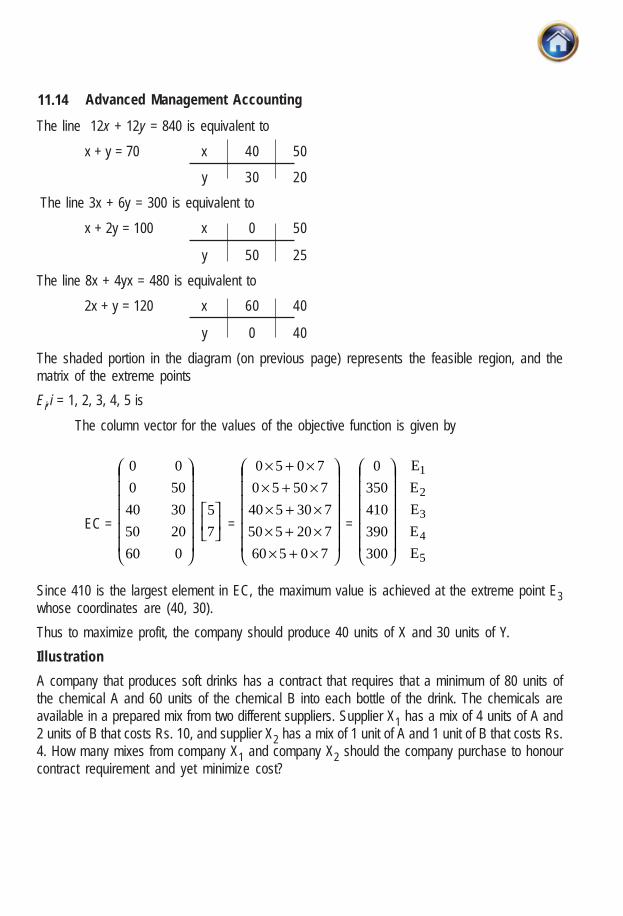
11.14 Advanced Management Accounting
The line 12x + 12y = 840 is equivalent to
x + y = 70 x 40 50
y 30 20
The line 3x + 6y = 300 is equivalent to
x + 2y = 100 x 0 50
y 50 25
The line 8x + 4yx = 480 is equivalent to
2x + y = 120 x 60 40
y 0 40
The shaded portion in the diagram (on previous page) represents the feasible region, and thematrix of the extreme points
Ei,i = 1, 2, 3, 4, 5 is
The column vector for the values of the objective function is given by
EC =
⎟⎟⎟⎟⎟⎟
⎠
⎞
⎜⎜⎜⎜⎜⎜
⎝
⎛
0
20
30
50
0
60
50
40
0
0
⎥⎦
⎤⎢⎣
⎡7
5 =
⎟⎟⎟⎟⎟⎟
⎠
⎞
⎜⎜⎜⎜⎜⎜
⎝
⎛
×+××+××+×
×+××+×
70560
720550
730540
75050
7050
=
5
4
3
2
1
E
E
E
E
E
300
390
410
350
0
⎟⎟⎟⎟⎟⎟
⎠
⎞
⎜⎜⎜⎜⎜⎜
⎝
⎛
Since 410 is the largest element in EC, the maximum value is achieved at the extreme point E3whose coordinates are (40, 30).
Thus to maximize profit, the company should produce 40 units of X and 30 units of Y.
Illustration
A company that produces soft drinks has a contract that requires that a minimum of 80 units ofthe chemical A and 60 units of the chemical B into each bottle of the drink. The chemicals areavailable in a prepared mix from two different suppliers. Supplier X1 has a mix of 4 units of A and2 units of B that costs Rs. 10, and supplier X2 has a mix of 1 unit of A and 1 unit of B that costs Rs.4. How many mixes from company X1 and company X2 should the company purchase to honourcontract requirement and yet minimize cost?

11.15Linear Programming
Solution
The problem may be summarized as follows:
Chemical Chemical Cost per mix
A B Rs.
Supplier X1 4 2 10
Supplier X2 1 1 4
Units required 80 60
Let x1 be the number of mixes to be purchased from supplier X1 and x2 be of those to bepurchased from supplier X2.
The conditions of the problem when symbolised, take the form:
Minimize Z = 10 x1 + 4 x2
Subject to the resrictions
x1 ≥ 0, x2 ≥ 0
4x1 + x
2 ≥ 80,
2x1 + x2 ≥ 60.
For the line 4x1 + x
2 = 80,
let x1 = 0, so that x2 = 80;
let x2 = 0, so that x1 = 20.
For the line 2x1 + x2 = 60,
let x1 = 0, so that x
2 = 60;
let x2 = 0, so that x1 = 30.
Feasible region is shaded in the diagram which appears to be unbounded. We now try to deter-mine the additional hidden conditions in the problem for which the feasible region becomesbounded.
Each bottle of the drink contains 80 units of the chemical A and 60 units of the chemical B. If thedrinks are made from the mixes of company X1 only, each bottle would require 20 mixes to meetthe chemical A requirement and 30 mixes to meet the chemical B requirement. Therefore, 30mixes would meet all minimum requirements. Any lesser amount of mixes would not meet theminimum requirement for chemical B.
Similarly, if the drinks are made from the mixes of company X2 only, each bottle would require 80mixes to meet both the chemical requirements.
��
��
��
2x + x = 60
1
2
4x+
x=
8 0
12
������
������
������
�������
������

11.16 Advanced Management Accounting
Since the company that manufac-tures drinks wants to make a blend-ing of the mixes purchased from boththe companies X1 and X2, it is pos-sible that the company would needless than the maximum amount ofboth supplies to meet the guaranteedminimum.
Thus we add the two additional hid-den conditions x1 ≤ 30, x2 ≤ 80.
With these two additional restrictionsthe above diagram takes the form :
x1 x2
The matrix of the extreme points, in this case, is E =
4
3
2
1
E
E
E
E
80
0
40
80
30
30
10
0
⎟⎟⎟⎟⎟
⎠
⎞
⎜⎜⎜⎜⎜
⎝
⎛
The column vector for the objective function is C = ⎟⎟⎠
⎞⎜⎜⎝
⎛4
10
2
1
x
x
The column vector for the values of the objective function is given by
EC = ⎟⎟⎟⎟⎟
⎠
⎞
⎜⎜⎜⎜⎜
⎝
⎛
80
0
40
80
30
30
10
0
⎥⎦
⎤⎢⎣
⎡4
10 =
⎟⎟⎟⎟⎟
⎠
⎞
⎜⎜⎜⎜⎜
⎝
⎛
×+××+××+××+×
4801030
401030
4401010
480100
=
4
3
2
1
E
E
E
E
620
300
260
320
⎟⎟⎟⎟⎟
⎠
⎞
⎜⎜⎜⎜⎜
⎝
⎛
Since 260 is the smallest element in EC, the minimum value is reached at the extreme point E2,whose coordinates are (10,40).
Thus, to honour the contract and yet to minimize cost, the company should purchase 10 mixesfrom X1 and 40 mixes from X2.
Summary of Graphical Method
It involves:
(i) Formulating the linear programming problem, i.e.,expressing the objective function andconstraints in the standardised format.
X 1
X = 301
E4
(3 0 ,8 0)E1
(0 ,8 0) X = 802
(0 ,6 0 )
2 x + x = 601 24 x + x = 801 2
O

11.17Linear Programming
(ii) Plotting the capacity constraints on the graph paper. For this purpose normally two terminalpoints are required. This is done by presuming simultaneously that one of the constraintsbis zero. When constraints concerns only one factor, then line will have only one originpoint and it will run parallel to the other axis.
(iii) Identifying feasible region and coordinates of corner points. Mostly it is done by breadingthe graph, but a point can be identified by solving simultaneous equation relating to twolines which intersect to form a point on graph.
(iv) Testing the corner point which gives maximum profit. For this purpose the coordinatesrelating to the corner point should put in objectives function and the optimal point shouldbe ascertained.
(v) For decision – making purpose, sometimes, it is required to know whether optimal pointleaves some resources unutilized. For this purpose value of coordinates at the optimalpoint should be put with constraint to find out which constraints are not fully utilized.
11.3 TRIAL & ERROR METHOD OF SOLVING LINEAR PROGRAMMING PROBLEM
11.3.1 Method of Solving LPP: Trial & Error Method (or Algebraic Approach)
Graphical method cannot be used when there are more than 2 variables in a LPP., in such acase we use the simplex method which is highly efficient and versatile as also amenable tofurther mathematical treatment and offers interesting economic interpretations. However, itsunderlying concepts are rather lengthy to discuss and the student should patiently go through thefollowing material on the trial and error method to gain a good grasp over the simplex technique.
Slack Variable
Consider the following example :
Example : Maximize Z = 3x1 + 4x
2
subject to 2x1 + 3x
2 + ≤ 16
4x1 + 2x2 ≤ 16
x1, x2 ≥ 0.
The ≤ type inequalities can be transformed into equalities by the addition of non negativevariables, say x3 and x4 (known as slack variables) as below. The slack variables represent idleresources, therefore, they are to be positive or non negative. Further the contribution per unit of aslack variable is always taken as zero in the objective function of a LPP. This is so because profitsare not made on unused resources.
⎭⎬⎫
⎩⎨⎧
=++=++
16124
16132
421
321
xxx
xxx...(A)
And the objective function may be rewritten as below.
Maximize Z = 3x1 + 4x
2 + 0x
3+ 0x
4

11.18 Advanced Management Accounting
Surplus Variable
In ³ type inequalities, we subtract a variable (called the surplus variable) to make it an equality.The value of this variable can be interpreted as the excess amount of the resources utilized overand above the given level. The contribution per unit of a surplus variable is also taken as zero inthe objective function.
11.3.2 The linear programming Theorems : The trial and error and simplex methods arebased on the concept of slack variables and theorems described below:
Extreme point theorem : It states that an optimal solution to a LPP occurs at one of the verticesof the feasible region. This should be obvious from the discussion on the graphical method.
Now the vertices are defined by the intersection of equations. The first step of the method is,therefore, to convert the inequalities into equalities by the addition (or subtraction) of the slack (orsurplus variables) depending on the direction of the inequality.
It is to be noted that the system of equations (A) above has more variables than the number ofequations. Such a system of equations has an infinite number of solutions; yet it has finite andfew vertices, the co-ordinates of which can be determined by applying the Basis theorem.
Basis theorem : It states that for a system of m equations in n variables (where n > m) has asolution in which at least (n-m) of the variables have value of zero as a vertex. This solution iscalled a basic solution.
Extreme point theorem can be extended to state that the objective function is optimal at least atone of the basic solutions. Some of the vertices may be infeasible in that they have -ve co-ordinates and have to be dropped in view of the non-negativity condition on all variables includ-ing the slack and surplus variables.
Consider the following LPP for elucidating the basis theorem.
Maximize Z = 3x1 + 4x2
Subject to 2x1 + 3x
2 < 16
4x1 + 2x2 < 16
x1 , x
2 >
0.
Introducing slack variables x3 and x4, we have
Maximize Z = 3x1 + 4x2 +0x3 + 0x4
Subject to 2x1 + 3x2 + 1x3 + 0x4 = 16
4x1 + 2x
2 + 0x
3 + 1x
4 = 16 ... (B)
x1 , x2 , x3 , x4 > 0.
Here n (number of variables) = 4 and m (number of equations) = 2. Thus n - m = 2. Accordingto the Basis theorem we set 2 (= n – m) variables in (B) equal to zero at a time, solve the resultingsystem of equations and obtain a basic solution. Thus if we zeroise x1 and x2, the resultingsystem of equations would be

11.19Linear Programming
⎭⎬⎫
⎩⎨⎧
=+=+
1610
1601
43
43
xx
xx......(C) Set 1 (x1
= x2 = 0)
These equations directly yield x3 = 16 and x4 = 16 as the basic solution i.e. the co-ordinate of avertex.
The other sets of equations, upon zeroising two variables at a time in (B), would be as follows:
⎥⎦
⎤⎢⎣
⎡=+=+
1624
1632
21
21
xx
xxSet 2 (x
3 = x
4 = 0)
⎥⎦
⎤⎢⎣
⎡=+=+1614
1602
41
41
xx
xxSet 3 (x2 = x3 = 0)
⎥⎦
⎤⎢⎣
⎡=+=+
1604
1612
31
31
xx
xxSet 4 (x2 = x4 = 0)
⎥⎦
⎤⎢⎣
⎡=+=+
1602
1613
32
32
xx
xxSet 5 (x
1 = x
4 = 0)
⎥⎦
⎤⎢⎣
⎡=+=+
1612
1603
42
42
xx
xxSet 6 (x1 = x3 = 0)
It is a simple matter to solve these six sets of simultaneous equations and obtain the six basicsolutions i.e. co-ordinates of the six vertices of the feasible region. The solutions are given below.The student may verify these by solving each of the sets of simultaneous equations.
Set Solution
1 x3 =16, x
4 = 16
2 x1 = 2, x2 = 4
3 x1 = 8, x
4 = –16
4 x1 = 4, x3 = 8
5 x2 = 8, x
3 = –8
6 x2 = 16/3, x4 = 16/3
Since solutions of set 3 and 5 yield a negative co-ordinate each, contradicting thereby the non-negativity of constraints, thus these are infeasible and are to be dropped from consideration.
Now according to the basis theorem the optimal solution lies at one of these vertices. By substi-tuting these co-ordinates the values of objective function are derived below:

11.20 Advanced Management Accounting
Set Solution Z (Profit)
1 x3 = 16, x4 = 16 0
2 x1 = 2, x
2 = 4 22
3 Infeasible
4 x1 = 4, x
3 = 8 12
5 Infeasible
6 x2 = 16/3, x
4 = 16/3 21
1
3
Thus solution of set 2 is optimal with a profit of 22. In this way we can solve a LPP simply byemploying the theorems stated above; but the simplex method is a further improvement over thetrial and error method. Following three are the inefficiencies in the trial and error method.
11.3.3 Inefficiencies of Trial and Error Method :
(a) In a LPP where m and n are larger, solving of numerous sets of simultaneous equationswould be extremely cumbersome and time-consuming.
(b) Scanning the profit table we notice that we jump from profit 0 to 22 to 211/3 i.e. there are upsand downs. The simplex method ensures that successive solutions yield progressively higherprofits, culminating into the optimal one.
(c) Some of the sets yield infeasible solutions. There should be means to detect such sets andnot to solve them at all.
11.4 THE SIMPLEX METHOD
The simplex method is a computational procedure - an algorithm - for solving linear programmingproblems. It is an iterative optimizing technique. In the simplex process, we must first find an initialbasis solution (extreme point). We then proceed to an adjacent extreme point. We continuemoving from point to point until we reach an optimal solution. For a maximization problem, thesimplex method always moves in the direction of steepest ascent, thus ensuring that the value ofthe objective function improves with each solution.
The process is illustrated with the help of the following example:
Illustration
Maximize Z = 3x1 + 4x
2
Subject to 2x1 + 3x
2 ≤ 16 (machining time)
4x1 + 2x
2 ≤ 16 (assembly time)
x1 ≥ 0, x2 ≥ 0

11.21Linear Programming
Solution
Step 1. Obtaining an initial solution: Obtain an initial solution that satisfies all the constraints ofthe problem. The simplex process requires that all constraints be expressed as equations. There-fore we must convert all inequalities into equalities.
Consider the constraint 2x1 + 3x2 < 16
Value on the left hand side of the inequality represents the amount of machine time a particularsolution uses, while the quantity on right side of inequality sign represents the total amount ofmachine time available. Let x3 be a variable which represents the unused machine time in thissolution so that
2x1 + 3x2 + x3 = 16
Similarly, let x4 represent the amount of assembly time that is available but not used so that
4x1 + 2x2 + x4 = 16
The variables x3 and x4 are referred to as slack variables.
Thus slack variables represent the quantity of a resource not used by a particular solution, andthey are necessary to convert the constraint inequalities to equalities.
As we proceed with the simplex method, it will be helpful to place certain information in a tableknown as a simplex tableau.
The simplex solution is as follows.
1 2 3 4 5 6
Fixed Program Profit Qty. 3 4 0 0 ReplacementRatio (basic Per unit x1 x2 x3 x4 Ratio
variables)
x3 0 16 2 3 1 0 16/3
I 2/3 x4 0 16 4 2 0 1 8
NER 3 4 0 0
1/4 x2 4 16/3 2/3 1 1/3 0 8
II x4 0 16/3 8/3 0 –2/3 1 2
NER 1/3 0 –4/3 0
III x2 4 4 0 1 1/2 –1/4
x1 3 2 1 0 –1/4 3/8
NER 0 0 –5/4 –1/8
The main simplex table, aside from headings, is seen divided into 3 horizontal sub-tables,I to III. There are 6 main headings 1 to 6 as explained below for sub-table I.

11.22 Advanced Management Accounting
Col. 1. Fixed ratio—explanation deferred.
Col. 2. Program —it contains the basic variables that are included in the solution. Initially, insub-table 1, there are slack variables, this means we do not produce x1 and x2 products,thus the profit is zero.
Col. 3. In the column labeled 'Profit' are listed the objective co-efficients of the basic variablesthat are included in the specific program. Thus, the profit co-efficients of x3 and x4 areall zero.
Col. 4. In the column labelled 'QTY' are listed the values of the basic variables included in thesolution. Since our initial program consists of 16 units of x3, and 16 units of x4, thesevalues are listed in 'QTY' column. Any variable which is not listed under the 'Program'column is known as the non-basic variable, the value of each non-basic variable iszero.
The total profit contribution resulting from a specific program can be calculated bymultiplying corresponding entries in the "profit per unit" column and the "quantity" columnand adding the product. Thus, total profit contribution in our first program is16(0) + 16(0) i.e. zero.
Col. 5. This heading is divided in as many sub-headings as the number of real and slackvariables. It indicates each of the variables with profit/unit as read from the objectivefunction at its top. The body of the sub-table carries the co-efficients of the variables asread from the constraints. That the co-efficients of the basic variables constitute a unitmatrix in this initial sub-table is to be noted. The numbers under the non basic variablesrepresent substitution ratio. For example, the number 2 gives the rate of substitutionbetween x1, and x3. If we wish to produce 1 unit of x1, 2 unit x3, must be sacrificed. Thenumber 4 has similar interpretation. To produce 1 unit of x1, 4 units of x4 must besacrificed. By using the same explanation, to produce 1 unit of x2 , we must sacrifice 3units of x3 and 2 units of x4.
Col. 6. Replacement ratio as discussed earlier.
The numbers in the net evaluation row (NER) Cj – Zj give the net effect of exchange betweenone unit of each variable and basic variable. They are always zero under the basic variables.Under the non-basic variables, they can be positive, negative or zero. Thus numbers in NER,under each column represent the opportunity cost of not having one unit of the respective columnvariable in the solution, in other words, the number represent the potential improvement in theobjective function that will result by introducing into the program one unit of the respective col-umn variable.
11.4.1 Test for Optimality : In so far as the total profit contribution (obtained by multiplyingcorresponding entries in the 'Profit' column and 'QTY' column and adding the product) resultingfrom the initial program is zero, it can be improved and hence is not optimal program. Inmaximization problem, the program is optimal if each Cj–Zj, is either zero or negative.
Computational aspects for the derivation of improved solutions are explained step by step below.

11.23Linear Programming
Step 1. Select the incoming variable in sub-table I in the NER. The NER entries in the first sub-table are simply the profit unit figures as read from the objective function or copied from headings5. However there is a more rigorous method of making these entries which alone has to befollowed in making entries in the subsequent NER's and explanation on which is deferred. Selec-tion of the incoming variable is simple indeed. The positive (Cj–Zj) in NER indicate the mag-nitude of opportunity cost of not including 1 unit of variables x1 and x2 respectively atthis stage. We select the one with highest entry in NER as incoming variable and thishappens to be x2, with a value of 4. We note this selection by putting an arrow below 4 in the NERof sub-table I. The column with the arrow is known as the key column.
Step 2. Select the outgoing variable, for this we have to calculate how many units of x2 can bebrought in without exceeding the existing capacity of any one of the resources? Thus, we mustcalculate the maximum allowable number of units of x2, that can be brought into the programwithout violating the non-negative constraints. For this, we compute the replacement ratio of col.6. This is done by dividing col. 4 by the key column and we get 16/3 and 8 and as the ratio. Thevariable x3, against the least ratio of 16/3 is selected as the outgoing variable and the fact is notedby putting an arrow against the least ratio of 16/3. This is maximum quantity of x2 that can beproduced at this stage without violating the non negative constraint. This row with the arrow iscalled the key row. The element at the intersection of the key row and the key column is knownas the pivot or key element and it is encircled.
Step 3. Having noted the incoming variable (x2 ) and the outgoing variable (x3 ) we are ready toperform the row operations on sub-table-I and fill in columns 4 and 5 of sub-table II.
Before that however, we fill in cols. 2 and 3 of sub-table II which is straight forward; x3 is replacedby x2 in col. 2, x4 stays in it and in col. 3 the profit/unit figure corresponding to x2 is copied fromheading while other figures remain the same.
11.4.2 Transformation of key row : The rule for transforming the key row is: Divide all thenumbers in the key row by the key number. The resulting numbers form the corresponding row inthe next table.
The key row of sub-table-I (under col. 4 and 5) is divided by the pivot element and this becomesthe corresponding row of the sub-table-II. It reads 16/3, 2/3, 1, 1/3, 0
11.4.3 Transformation of the non-key rows : The rule for transforming a non-key row is:Subtract from the old row number (in each column) the product of the corresponding key-rownumber and the corresponding fixed ratio formed by dividing the old row number in the keycolumn by the key number. The result will give the corresponding new row number.
This rule can be placed in the following equation form:
Fixed ration = numberkey
columnkeyinnumberrowOld
These are entered in the non key row under column I in the sub-table-I itself.
New row number = old row number
– (corresponding number in key row × corresponding fixed ratio)

11.24 Advanced Management Accounting
The key row in sub-table-I is multiplied by the fixed ratio of the non key row. This leads to
162
3
32
32
2
3
4
33
2
32 1
2
3
2
30
2
30× = × = × = × = × =, , , ,
This, however, is a rough work. Entries are not made any where. The result of this multiplicationare subtracted from the non-key row of sub-table-I to yield the non key row of the sub-table-II asbelow:
16 – 32
3 =
163
, 4 –43
= 8
3, 2 – 2 =0, 0 –
23
= – 23
, 1–0 = 1
These entries are made for the non-key row of sub-table-II.
Step IV. This consists of deriving the NER of sub-table-II. Each of its elements is derived bymultiplying col. 3 of sub-table-II with col. 5, summing these up and subtracting the sum from theprofit/unit is heading 5. Computations for each element in the 2nd NER are shown below:
3
1
3
80
3
243 =⎟
⎠⎞⎜
⎝⎛ ×+×−
4 – (4 × 1 + 0 × 0) = 0
3
4
3
20
3
140 −=⎟
⎠⎞⎜
⎝⎛ −
×+×−
0 – (4 × 0 + 0 × 1) = 0
But what is the underlying logic? The constraints in the sub-table – II have become
2
3x x x x1 2 3 4+ 1 +
1
3+ 0 =
16
3
8
3x
1 +0x
2 –
2
3 x
3 + 1x
4=
16
3
i.e. x2
=16
3–
2
3x
1–
1
3x
3(i)
x4 =
16
3–
8
3x
1+
2
3x
3(ii)
Substituting these values of x2 and x
4 in the original objective function
Z = 3x1 + 4x
2 + 0x
3 + 0x
4

11.25Linear Programming
We get the following modified function,
Z = 3x1 + 4 ⎭⎬⎫
⎩⎨⎧ −− 31 3
1
3
2
3
16xx
+ 0x3 + 0⎭⎬⎫
⎩⎨⎧ +− 31 3
2
3
8
3
16xx
= x1 ⎭⎬⎫
⎩⎨⎧ ×−×− 0
3
84
3
23 + 0x2 + x3 ⎭
⎬⎫
⎩⎨⎧ ×+×−
3
20
3
140 + 0x4 + 4 ×
16
3
i.e. , Z = 1
3x1 + 0x2 –
43
x3 + 0x4 + 643
These co-efficients have been entered in the 2nd NER
[This might appear to be mathematical jugglery but there is a sound interpretation to this.]
The reason for this becomes clear if we keep in mind that 13 x1 + 0x2–
43 x3 + 0x4 + 64
3
becomes the modified objective function corresponding to the solution stage given by the program2 i.e. , sub-table-II, that has fully utilised the machining capacity. Thus the production of 1 unit ofX
1 at this stage will mean (according to the 1st original constraint 2x
1 +3x
2 ≤ 16) that 2 units of
machining capacity (required for producing 1 unit of X1) must be reallocated from X
2. Since each
unit of X2 requires 3 units of machining capacity, current level of production will thus be reduced
by 23 unit which will mean reduction of Rs. 8
3 (= 4 × 23 ) in the contribution. Thus, introduction
of 1 unit of X1 at this stage results in a decrease of Rs. 8
3 in the profit contribution of X2. Hence
the introduction of 1 unit X1 at this stage will give a net profit i.e., of 3 – 83 = Rs. 1
3 Similar
interpretation can be made for the co-efficients in the modified objective function].
By applying these 4 steps on sub-table-II we derive sub-table-III. Since its NER does not have anypositive element i.e. opportunity cost, we stop here. This is an indication of the optimal solutionwith x1=2 and x2 = 4 (and Z = 22), for if we derive another sub-table by bringing in x3 or x4 into thesolution we shall decrease the profit. To sum up, when, in a maximization problem, all theelements in an NER are negative or zero we stop further iterations. The student may himselfderive sub-table-III as an exercise.
It is obvious that the student needs a plenty of practice to be thorough with the computationallytedious though otherwise very elegant and versatile simplex method. As a tip, the fractions in thesimplex tables must be retained and by trying to decimalise them the student may land himself introuble. Numerous examples and exercises follow to give understanding and practice to thestudents.
Illustration
An electronics firm is undecided as to the most profitable mix for its products. The products nowmanufactured are transistors, resistors and carbon tubes with a profit (per 100 unit) of Rs. 10, Rs.

11.26 Advanced Management Accounting
6 and Rs. 4 respectively. To produce a shipment of transistors containing 100 units requires 1hour of engineering, 10 hours of direct labours and 2 hours of administrative service. To produce100 resistors are required 1 hour, 4 hours and 2 hours of engineering, direct labour and admin-istrative time respectively. To produce on shipment of the tubes (100 units) requires 1 hour ofengineering, 5 hours of direct labour and 6 hours of administration. There are 100 hours ofengineering services available, 600 hours of direct labour and 300 hours of administration. Whatis the most profitable mix?
Solution
Let us tabulate the data in convenient manner.
Products
Transistors Resistors Carbon Tubes Availability
Engineering 1 1 1 100
Labour 10 4 5 600
Admnstraton 2 2 6 300
Profit (per 100 units) (Rs.) 10 6 4
Symbolically, Maximize 10x + 6y + 4z
here x, y, z represents units of Transistors, Resistors and Carbon tubes (in 100 units)
Subject to 1x + 1y + 1z ≤ 100 and x ≥ 0
10x + 4x + 5z ≤ 600 and y ≥ 0
2x + 2y + 6z ≤ 300 and z ≥ 0
Introducing slack variables
Maximize 10x + 6y + 4z
Subject tox + y + z + S1 = 100
10x + 4y + 5z + S2 = 600
2x + 2y + 6z + S3 = 300
x ≥ 0, y ≥ 0, z ≥ 0, S1 ≥ 0, S
2 ≥ 0, S
3 ≥ 0
P ro g -
ra m
P ro fit/
U n it
Q ty . 1 0
x
6
y
4
z
0
S 1
0
S 2
0
S 3
R e p la c e m e n t
R a tio
S 1 0 1 0 0 1 1 1 1 0 0 1 0 0F .R = 1 /1 0
S 2 0 6 0 0 1 0 4 5 0 1 0 6 0 ←_
1 /5 S 3 0 3 0 0 2 2 6 0 0 1 1 5 0
N e t E v a lu a tio n R o w 1 0 6 4 0 0 0

11.27Linear Programming
Hence the most profitable mix is y = 4006 Resistors and x = 100
3 Transistors. The maximum
profit is 400 + 10003 = 733 1
3
11.5 SIMPLEX METHOD FOR MINIMIZATION PROBLEMS
The simplex algorithm applies to both maximization and minimization problems. The onlydifference in the algorithm involves the selection of the incoming variable. In the maximizationproblem it is the one with highest +ve NER element. Conversely, it is the most – ve variable thatis selected as the incoming variable in a minimization problem. And if all elements in the NERare either positive or zero, it is the indication for the optimal solution and we stop there.
Let us take an example straightway to explain the solution procedure.
Illustration
A small township of 15,000 people requires, on the average, 300,000 gallons of water daily. Thecity is supplied water from a central water-works where the water is purified by such conventionalmethods as filteration and chlorination. In addition, two different chemical compounds : (i) softeningchemical and (ii) health chemical, are needed for softening the water and for health purposes.The waterworks plans to purchase two popular brands that contain these chemicals. One unit ofChemico Corporation's product gives 8 pounds of softening chemical and 3 pounds of healthchemical. One unit of Indian Chemical's product contains 4 pounds and 9 pounds per unit,respectively, for the same purposes.
To maintain the water at a minimum level of softness and to meet a minimum programme ofhealth protection, experts have decided that 150 and 100 pounds of the two chemicals thatmake up each product must be added to water daily. At a cost of Rs. 8 and Rs. 10 per unitrespectively for Chemico's and Indian Chemical's products, what is the optimal quantity of eachproduct that should be used to meet the minimum level of softness and minimum health stand-ard?
S1 0 40 0 6/10 5/10 1 –1/10 0 400/6=67
F.R =2/3 x 10 60 1 4/10 5/10 0 1/10 0 600/4=150
F.R.=2 S3 0 180 0 12/10 5 0 –2/10 1 150
Net Evaluation Row 0 2
↑
–1 0 –1 0
X1
y 6 400/6 0 1 5/6 10/6 –1/6 0
x 10 100/3 1 0 1/6 –2/3 1/6 0
S3 0 100 0 0 4 –2 0 1
Net Evaluation Row 0 0 – ve –ve –ve 0

11.28 Advanced Management Accounting
Solution
The relevant data may be tabulated as below :
Brand
Chemical Chemico Indian Daily Requirement
(i) Softening 8 4 150
(ii) Health 3 9 100
Cost/Unit of each brand (Rs.) 8 10
Let us formulate the LPP as below
Minimize (cost), Z = 8x + 10y
Subject to
8x + 4y ≥ 150
3x + 9y ≥ 100
and x ≥ 0, y ≥ 0
Here x and y represents units of softening and health chemical units respectively.
Subtracting surplus variables to convert inequalities into equalities.
8x + 4y - S1 = 150
3x + 9y - S2 = 100
11.5.1 Physical Interpretation of Surplus Variables : Let S1 and S2 represent the extra units(if any) of the two chemicals over 150 and 100 units respectively. Their magnitude being such asto just convert the inequalities into equalities, thereby restricting them to non-negative value. Theproblem may then be restated as below:
Minimise (cost) Z = 8x + 10y + 0S1 + 0S2
Subject to 8x + 4y - S1 = 150
3x + 9y - S2 = 100
and S1 ≥ 0, S2 ≥ 0, x ≥ 0, y ≥ 0.
11.5.2 Artificial Slack Variables : If x and y are set equal to zero S1 and S
2 turn out to be
negative, violating the non-negativity restriction. Therefore, to circumvent this, we introduce anothersimilar device of artificial slack variables. Let us represent these by A
1 and A
2 respectively. The
problem then becomes :
Minimize cost Z = 8x + 10y + 0S1 + 0S
2 + MA
1 + MA
2
Subject to⎭⎬⎫
⎩⎨⎧
=+−+=+−+
100AS93
150AS48
22
11
yx
yxAll variables > 0

11.29Linear Programming
Physical Interpretation of the Artificial Variables.
These are imaginary brands, each unit containing 1 unit of the pertinent chemical. Both arerestricted to non-negatives. Whereas surplus variables have zeros as their cost co-efficient, eachartificial variable is assigned an infinitely large cost co-efficient (usually denoted by M).
Uses of artificial variables
1. It is our basic assumption that none of the basic variables in the L.P. problem can have anegative value. Thus, artificial variable is added to act as basic variable in a particularequation and hence it avoids the possibility of getting negative values for basic variables.
2. These artificial variables are such that their objective function co-efficients impose a hugeand hence unacceptable penalty. In the case of maximization problem, the objective functionis modified by subtracting a quantity (MA1) where M is arbitrarily large value and A1 is theartificial variable. For minimization problem, the objective function is modified by adding thequantity MA1. Thus artificial variables enable us to make a convenient and correct start inobtaining an initial solution.
3. The artificial variables with the high penalty once replaced by a real variable will never enterthe optimal program. Hence the solution to the modified problem will give the optimal solu-tion to the original problem.
11.5.3 Designing the Initial Program : It is obtained by letting each of the variables x,y, S1 and
S2 assume value of zero, i.e., retaining artificial variables in the initial solution.
11.5.4 Initial Solution : It is to be noted that in the NER we do not copy the co-efficients from thecost objective but derive them by step IV of Section 14.4.3 as below :
x 8–8M – 3M = 8–11M
y 10–4M – 9M = 10–13M
S1 0 + M – 0 = M
S2
0 – 0 + M = M (A)
A1 M – M – 0 = 0
A2
M – 0– M = 0
Prog
ram
Cost per
Unit
Qty. 8
x
10
y
0
S1
0
S2
M
A1
M
A2
Replacement
Ratio
A1 M 150 8 4 –1 0 1 0 150/4
A2 M 100 3 9 0 –1 0 1 100/9←
Net Evaluation Row 8–11M 10–13M M M 0 0

11.30 Advanced Management Accounting
The reason for this is explained below. The problem is rewritten below:
Minimize Z = 8x + 10y + 0S1+ 0S
2 + MA
1 + MA
2
Subject to 8x + 4y – S1 + A1= 150 ... (i)
3x + 9y – S2 + A2= 100 ... (ii)
All variables ≥ 0.
From (i) A1 = 150 – 8x – 4y + S
1
From (ii) A2 = 100 – 3x – 9y + S2
Substituting these in the objective function,
Z = 8x + 10y + 0S1 + 0S
2+ M (150–8x – 4y + S
1) + M(100 – 3x – 9y + S
2)
= (8 – 11M) x + (10 – 13M) y + MS1+ MS
2+ 0A
1+ 0A
2.
These co-efficients correspond to set A above.
Now consider the initial solution with an initial cost of (150 + 100) M for further inspiration.
10–13M is the most – ve and, therefore, the column, under 'y' is the key column. Also, the ratio100/9 is less than 150/4 (on extreme right). The pivot element, then, is 9. The outgoing variableis A2 being replaced by y. The cost of the existing solution, 250 M is forbiddingly high. The stageis set for revising the initial program.
The key row is revised by dividing it through by 9, the pivot element and the results are as follows:
1003
, 39
, 1,0, -1
9, 0,
19
.
The fixed ratio for revising the non-key row is 4/9. The revised figures for this row are computedbelow:
150 – 100 × 49
= 1350 400
9
950
9
– =
8 – 3 × 9
4 =
9
1272 − =
9
6
4 – 9 × 49
= 0
– 1 – 0 = –1
0 + 49
= 4
91 – 0 = 1
0 – 1 × 49
= 9
4−

11.31Linear Programming
The new table is shown below:
Revising the key row by dividing it through by 60
9 i.e. multiply by
9
60, we get
950
60, 1, 0,
–9, , ,
–
60
4
60
9
60
4
60
For the non-key row the fixed ratio is 3/9 ¸ 60/9 = 3/60. Revising the non-key row.
100
9
950
9
3
60
35
6– × =
3
9
60
9
3
600– × =
13
6 00 1– × =
0 13
60
1
20+ × =
–1
9
4
9
3
60 15–
–2× =
03
60
1
20– –=
1
9
4
9
3
60
2
15+ × =
Prog
ram
Cost/
Unit
Qty. 8
x
10
y
0
S1
0
S2
M
A1
M
A2
A1 M 950/9 60/9 0 –1 4/9 1 –4/9 950/60←
y 10 100/9 3/9 1 0 –1/9 0 1/9 100/3
Net Evaluation Row 42/9–
60M/9 0 M
10/9–
4M/9 0
13M–10
9

11.32 Advanced Management Accounting
The result are tabulated below:
Hence the optimal cost is 95
68
35
610× + ×
= 760 350
3+
= 1110
6 = 185 Answer.
11.6 MARGINAL VALUE OF A RESOURCE
Let us consider the first example under section 15.4 once again to explain this concept. In thesaid example there are two resources machining and assembly. The optimal tableau of thatexample is reproduced below. We see in its NER -5/4 and –1/8 below x3 and x4. The marginalvalue of the machining and assembly resources are then respectively 5/4 and 1/8. The implica-tion of this is that if now (at the optimal stage) we wish to bring in x3 in the solution, the total profitwill be reduced from 22 (the optimal) by 5/4 times the no. of units of x3 brought in the program.This is demonstrated below where we bring x3 in this program.
Optimal table of first Example in Section 15.4 follows (rest omitted). x3 is brought in the next tooptimal table.
*Profit has been reduced from 22 to 12 because 8 units of x3 have been brought in the new solution, thereby the net reductionof profit 10 naturally equals 8 × 5/4.
Prog
ram
Cost/
Unit
Qty. 8
x
10
y
0
S1
0
S2
M
A1
M
A2
x 8 95/6 1 0 –3/20 1/15 3/20 –1/15
y 10 35/6 0 1 1/20 –2/15 –1/20 2/15
NER (all non-negative) 0 0 7/10 4/5 M– 7/10 M–4/5
1/2
x2
x1
4
3
4
2
x1
0
1
x2
1
0
x3
1/2
–1/4
x4
–1/4
3/8
8�
–8
Optimal NER 22* 0 0 –5/4 –1/8 Bring x3 insolution
X3
x1
0
3
8
4
0
1
2
1/2
1
0
–1/2
1/4
12* 0 0 5/2 0 –3/4
x3

11.33Linear Programming
Please note that marginal value of resource is synonymous with opportunity cost or shadow price.
11.7 SOME REMARKS
1. It may be desired to convert a maximization problem into a minimization one and viceversa. Mathematically, this can be accomplished by reversing signs though of just theobjective function.
2. Inequalities in the wrong direction: Consider the problem:
Maximize Z = x1 + 5x2
Subject to 3x1 + 4x
2 ≤ 6 ... (i)
x1 + 3x
2 ≥ 2 ... (ii)
x1 , x2 ≥ 0[Whether to introduce slack or surplus or artificial variables depends on the type ofinequality and has nothing to do with type of the problem i.e., maximization orminimization].
The 2nd inequality is in the wrong direction. Upon introducing the "surplus" variable.
x1 + 3x2 – S2 = 2
If S2 is taken in the initial solution it would be – ve when x1 and x2 are zero. To circumvent this,an artificial variable is also introduced in this inequality. The problem becomes:
Maximize Z = x1 + 5x2 - MA2
Subject to 3x1 + 4x2 + S1 = 6
x1 + 3x2 – S2 +A2 = 2
x1 , x
2, S
1, S
2, A
2 > 0
(Note that in maximization problems M always has -ve sign and in minimization problemsM always has a + ve sign in the objective function).
The initial solution consists of S1 and A2. Several examples on inequalities in the wrong directionfollow. Surplus variables can never come in initial solution.
3. Any linear programming problem can be re-formulated into what is known as its dual. Any ofthe primal (the original) or the dual may be selected for iterating by the simplex method. Theselection is made on the basis of computational burden. Also the dual provides interestinginsights into the methodology of the LP solution. This matter is discussed in a followingsection at a greater length.
4. If two or more variables share the maximum positive co-efficient in the net evaluation row anyone may be chosen for introduction for the new solution arbitrarily, viz., in Z = 2x1 + 2x2 + x3it matters little if x1 or x2 is chosen.
5. Lower bounds may be specified in an LPP. For example, over and above to the three usualconstraints, it may be stipulated that x1 cannot be less than 25 or 40 or l1.i.e., x1 > l1. This can

11.34 Advanced Management Accounting
be handled quite easily by introducing a variable y1 such that x1 = l1 + y1. Substitute x1 = l1+ y1 wherever it occurs and solve the LPP. Computations would be greatly reduced. Pleasesee illustration on page no. 15.32 in this connection.
6. In all the simplex tables there is bound to be a unit matrix of size p × p where p is the no. ofrows (excluding net evaluation row). The columns that constitute such a unit matrix need notbe adjacent.
7. In view of the tediousness of computational aspects it is useful to make a check at eachiteration. This can be done by deriving the net evaluation row in two ways. (i) just like anyother row in the simplex tableau by deriving its fixed ratio (ii) by summing the product of thequantities column with the profit/cost column and subtracting this sum from the original profitcontribution or cost co-efficient of variable. These should tally. Also, having obtained theoptimal solution it is desirable to verify it if it obeys the given constraints.
8. The simplex method, the graphical and trial and error methods, the dual approach provideseveral ways of doing an LPP. The student may want to do each LPP in more than one wayfor the sake of verification of the answer and practice.
Illustration
A manufacturer of three products tries to follow a policy of producing those which contribute mostto fixed cost and profit. However, there is also a policy of recognising certain minimum salesrequirements. Currently these are:
Product Unit per week
X 20
Y 30
Z 60
There are three producing departments. The product time in hour per unit in each departmentand the total times available for each week in each department are:
Time required per product, in hours Total hours available
Product X Y Z
Department 1 0.25 0.20 0.15 420
2 0.30 0.40 0.50 1,048
3 0.25 0.30 0.25 529
The contribution per unit of product X,Y, Z is Rs. 10.50, Rs. 9.00 and Rs. 8.00 respectively. Thecompany has scheduled 20 units of X, 30 units of Y and 60 units of Z for production in thefollowing week.
You are required to state:
(a) Whether the present schedule is an optimum one from a profit point of view and if it is not,what it should be;

11.35Linear Programming
(b) The recommendations that should be made to the firm about their production facilities(following the answer to (a) above).
Solution
Let us formulate the L.P.P.
Objective: Maximize 10.50X + 9.00Y + 8.00Z
Subject to 0.25X + 0.20Y + 0.15Z ≤ 420
0.30X + 0.40Y + 0.50Y ≤ 1048
0.25X + 0.30Y + 0.25Z ≤ 529
0 ≤ X > 20 0 ≤ X means
0 ≤ Y > 30 X ³ 0, etc.
0 < Z > 60
Since the company is already producing minimum of Y and Z it should, at least, produce maxi-mum of X limited by the first constraint. It can be arithmetically verified that there is a scope forimprovement.
Substituting (Please refer to point 5 in Section 15.7) :
X = x1 + 20
Y = x2 + 30
Z = x3 + 60
This problem becomes
Maximize 10.50x1 + 9.00 x2 + 8.00 x3 + a constant
Subject to 0.25 x1 + 0.20x2 + 0.15x3 ≤ 400
0.30 x1 + 0.40x
2 + 0.50x
3 ≤ 1000
0.25 x1 + 0.30x2 + 0.25x3 ≤ 500
x1 ≥ 0, x
2 ≥ 0, x
3 ≥ 0
The student may now derive the optimal solution, as an exercise.
� Miscellaneous Illustrations
Illustration
The owner of Fancy Goods Shop is interested to determine, how many advertisements to re-lease in the selected three magazines A,B and C. His main purpose is to advertise in such a waythat exposure to principal buyers of his goods is maximized. Percentages of readers for eachmagazine are known. Exposure in any particular magazine is the number of advertisementsreleased multiplied by the number of principal buyers. The following data are available:

11.36 Advanced Management Accounting
Magazines
Particulars A B C
Readers 1.0 lakh 0.6 lakh 0.4 lakh
Principal Buyers 20% 15% 8%
Cost per Advertisement 8,000 6,000 5,000
The budgeted amount is at the most 1.0 lakh for the advertisement. The owner has alreadydecided that magazine A should have no more than 15 advertisements and that B and C eachgets at least 8 advertisements. Formulate a Linear Programming Model for this problem.
Solution
Let x1, x2 and x3 denote the number of advertisements to be released in three magazines A, B andC respectively. Let Z denote the total exposure to the principal buyers of the goods.
Since the exposure in any magazine is the number of advertisements multiplied by the number ofprincipal buyers, therefore, the value of Z is given by :
Z = (0.20 × 1,00,000) x1 + (0.15×60,000) x2 + (.08 × 40,000) x3
= 20,000 x1 + 9000 x2 + 3,200 x3
The owner of Fancy Goods shop wishes to maximise the total exposure to principal buyers,hence the objective function is given by
Maximize Z = 20,000 x1 + 9,000 x
2 + 3,200 x
3
subject to the following constraints :
(i) The budgeted amount for the advertisement is at the most Rs. 1,00,000.
Hence, 8,000 x1 + 6,000 x
2 + 5,000 x
3 ≤ 1,00,000.
(ii) Also, the magazine A should have no more than 15 advertisements, B and C each should getat least 8 advertisements.
Hence, x1 ≤ 15
and x2 ≥ 8, x3 ≥ 8
Thus, the linear programming model for the problem is
Maximise Z = 20,000 x1 + 9,000 x2 + 3,200 x3
subject to
8,000 x1 + 6,000 x2 + 5,000 x3 ≤ 1,00,000
x1 ≤ 15, x
2 ≥ 8, x
3 ≥ 8
Where x1, x
2, and x
3 ≥ 0.

11.37Linear Programming
Illustration
A Mutual Fund Company has Rs. 20 lakhs available for investment in Government Bonds, bluechip stocks, speculative stocks and short-term deposits. The annual expected return and riskfactor are given below:
Type of investment Annual Expected Return (%) Risk Factor (0 to 100)
Government Bonds 14 12
Blue Chip Stocks 19 24
Speculative Stocks 23 48
Short-term Deposits 12 6
Mutual fund is required to keep at least Rs. 2 lakhs in short-term deposits and not to exceedaverage risk factor of 42. Speculative stocks must be at most 20 percent of the total amountinvested. How should mutual fund invest the funds so as to maximize its total expected annualreturn? Formulate this as a Linear Programming Problem. Do not solve it.
Solution
Let x1, x2, x3 and x4 denote the amount of funds to be invested in government bonds, blue chipstocks, speculative stocks and short term deposits respectively. Let Z denote the total expectedreturn.
Since the Mutual Fund Company has Rs. 20 lakhs available for investment,
x1+ x
2+ x
3+ x
4 ≤ 20,00,000 ... (i)
Also, Mutual fund is required to keep at least Rs. 2 lakhs in short-term deposits,
Hence, x4 ≥ 2,00,000 ...(ii)
The average risk factor is given by
12x1 + 24x
2 + 48x
3 + 6x
4
x1 + x2 + x3 + x4
Since the average risk factor Mutual Fund should not exceed 42, we get the following constraint.
12x1 + 24x
2 + 48x
3 + 6x
4
x1 + x
2 + x
3 + x
4 ≤ 42
or 12x1 + 24x2 + 48x3 + 6x4 ≤ 42 (x1+x2+x3+x4)
or –30x1 – 18x
2 + 6x
3 – 36x
4 ≤ 0 ...(iii)

11.38 Advanced Management Accounting
Further, speculative stock must be at most 20 per cent of the total amount invested, hence
x3 ≤ 0.20 (x
1 + x
2 + x
3 + x
4)
or – 0.2x1 – 0.2 x2 – 0.8x3– 0.2x4 ≤ 0 ...(iv)
Finally, the objective is to maximise the total expected annual return, the objective function forMutual Fund can be expressed as
Maximise Z = 0.14x1 + 0.19x2 + 0.23x3 + 0.12x4 ...(v)
Summarising equations (i) to (v), the linear programming model for the Mutual Fund company isformulated as below:
Objective function :
Maximize Z = 0.14x1 + 0.19x2 + 0.23x3 + 0.12x4
Subject to the constraints
x1
+ x2
+ x3
+ x4 ≤ 20,00,000
x4 ≥ 2,00,000
– 30x1 – 18x2 + 6x3 – 36x4 ≤ 0
– 0.2x1 – 0.2x
2+ 0.8x
3 – 0.2x
4 ≤ 0
where x1 ≥ 0, x2 ≥ 0, x3 ≥ 0 and x4 ≥ 0
Illustration
A firm produces three products A, B and C. It uses two types of raw materials I and II of which5,000 and 7,500 units respectively are available. The raw material requirements per unit of theproducts are given below:
Raw Material Requirements per unit of Product
A B C
I 3 4 5
II 5 3 5
The labour time for each unit of product A is twice that of product B and three times that ofproduct C. The entire labour force of the firm can produce the equivalent of 3,000 units. The(marks) minimum demand of the three products is 600, 650 and 500 units respectively. Also, theratios of the number of units produced must be equal to 2 : 3 : 4. Assuming the profits per unit ofA,B and C as Rs. 50, 50 and 80 respectively.
Formulate the problem as a linear programming model in order to determine the number of unitsof each product which will maximize the profit.

11.39Linear Programming
Solution
Let the firm produce x1 units of product A, x2 units of products B and x3 units of product C.
The profit per unit of products A, B and C is Rs. 50, and Rs. 80 respectively. Since the objectiveof the firm is to maximize the profit, therefore, the objective function is given by
Maximise Z = 50x1 + 50x2 + 80x3
The firm uses two types of raw materials I and II of which 5,000 and 7,500 units respectively areavailable. As per the given data, the raw material constraints can be formulated as given below:-
3x1 + 4x2 + 5x3 ≤ 5,000 ...(i)
and 5x1 + 3x2 + 5x3 ≤ 7,500 ...(ii)
The labour time for each unit of product A is twice that of product B and three times thatof product C. Also the entire labour force can produce the equivalent of 3000 units.
∴ xx x
12 3
2 33000+ + ≤
or 6x1 + 3x
2 + 2x
3 ≤ 18000 ...(iii)
The minimum demand of the three products is 600, 650 and 500 units respectively.
Hence, x1 ≥ 600, x2 ≥ 650 and x3 ≥ 500 ...(iv)
Since the ratios of the number of units produced must be equal to 2 : 3 : 4, therefore,
1/2 x
1= 1/
3 x
2, and 1/
3 x
2 = 1/
4 x
3
or 3x1 = 2x
2 and 4x
2 = 3x
3...(v)
The linear programming model can be formulated as follows:
Maximise Z = 50x1 + 50x
2 + 80x
3
Subject to the constraints :
3x1 + 4x
2 + 5x
3 ≤ 5000
5x1 + 3x
2 + 5x
3 ≤ 7500
6x1 + 3x
2 + 2x
3 ≤ 18000
3x1 = 2x2 and 4x2 = 3x3
x1 ≥ 600, x2 ≥ 650 and x3 ≥ 500.

11.40 Advanced Management Accounting
11.8 PRACTICAL APPLICATIONS OF LINEAR PROGRAMMING
In addition to its wide use in industrial and administrative applications, linear programming hasextensive application to agricultural, aircraft and several military problems. These are brieflydiscussed below. The student need not memories the numerical examples. They are givenmerely to enhance understanding of applications. However, he is advised to keenly study theformulation of various LPPs given as examples.
Illustration
For a company engaged in the manufacture of three products viz., X, Y and Z, the available dataare give in Tables 1, 2 and 3 below:
Table 1 : Minimum sales requirements
Product Minimum Sales
Requirements per month
X 10
Y 20
Z 30
Table 2 : Operations, Required Processing Times and Capacity
Operations Time (Hrs) required per item of Total available
X Y Z hours per month
1 1 2 2 200
2 2 1 1 220
3 3 1 2 180
Table 3 : Profit (Rs.) per unit
Product Profit (Rs.)/Unit
X 10
Y 15
Z 8
Find out the product mix to maximize profit.
Solution
Let x, y and z denote the number of units produced per month for the products X, Y and Zrespectively.

11.41Linear Programming
Minimum sales requirements give following constraints :
x ≥ 10
y ≥ 20 where x, y, z ≥ 0
z ≥ 30
Operations, processing times and capacity lead to following constraints:
x + 2y + 2z ≤ 200
2x + y + z ≤ 220
3x + y + 2z ≤ 180
The objective function is
Maximize 10x + 15y + 8z
Thus, we have to solve the following problem
Maximize P = 10x + 15y + 8 z
Subject to x + 2y + 2z ≤ 200 ................................................................... (i)
2x + y + z ≤ 220 ................................................................. (ii)
3x + y + 2z ≤ 180 ................................................................ (iii)
x ≥ 10 ................................................................................... (iv)
y ≥ 20 .................................................................................... (v)
z ≥ 30 ................................................................................... (vi)
x,y,z, ≥ 0.
Let us make following substitutions
x = a + 10
y = b + 20
z = c + 30
Where a, b, c ³ 0.
Substituting these values in the objective function and constraints (i), (ii), & (iii), the problembecomes
Maximize P = 10a + 15b + 8c + 640
subject to (a + 10) + 2(b + 20) + 2(c + 30) ≤ 200
2(a + 10) + (b + 20) + (c + 30) ≤ 220
3(a + 10) + (b + 20) + 2 (c + 30) ≤ 180
where a,b,c ≥ 0
or Maximize P = 10a + 15b + 8c + 640

11.42 Advanced Management Accounting
subject to a + 2b + 2c ≤ 90
2a + b + c ≤ 150
3a + b + 2c ≤ 70
where a,b,c ≥ 0.
Adding slack variables S1, S2, and S3, we get
Maximize P = 10a + 15b + 8c + 640 + 0S1 + 0S
2 + 0S
3
Subject to a + 2b + 2c + S1 = 90
2a + b + c + S2 = 150
3a + b + 2c + S3 = 70
The initial feasible solution is obtained by setting a = b = c = 0. The solution is S1 = 90, S2 = 150,S3 = 70, P = 640. This solution and further improved solutions are presented in following matrixform:
Since all NER elements are less than or equal to zero, the previous table gives the optimalsolution. The solution is
a = 10, b = 40 and c = 0Substituting these values
x = 10 + 10 = 20, y = 40 + 20 = 60,z = 0 + 30 = 30
and the value of objective function is given byP = Rs. 10 × 20 + Rs. 15 × 60 + Rs. 8 × 30 = Rs. 200 + Rs. 900 + Rs. 240
= Rs. 1340
Prog. Profit Qty 10a
15b
8c
0S1
0S 2
0S3
Replacementratios
S1
S2
S3
000
9015070
123
211
212
100
010
001
4515070
10 15 8 0 0 0
bS 2
S3
1500
4510525
1/23/25/2
100
101
1/2–1/2–1/2
010
001
907010
5/2 0 –7 –15/2 0 0b 15 40 0 1 4/5 3/5 0 –1/5S2 0 90 0 0 –3/5 –1/5 1 –3/5a 10 10 1 0 2/5 –1/5 0 2/5
0 0 –8 –7 0 –1
↑
↑

11.43Linear Programming
The optimal product mix is to produce 20 units of X, 60 units of Y and 30 units of Z to get a profitof Rs. 1340.
Illustration
The Delhi Florist Company is planning to make up floral arrangements for the upcoming festival.The company has available the following supply of flowers at the costs shown:
Type Number available Cost per flower
Red roses 800 Rs. 0.20
Gardenias 456 Rs. 0.25
Carnations 4,000 Rs. 0.15
White roses 920 Rs. 0.20
Yellow roses 422 Rs. 0.22
These flowers can be used in any of the four popular arrangements whose makeup and sellingprices are as follows:
Arrangement Requirements Selling price
Economy 4 red roses Rs. 6
2 gardenias
8 carnations
May time 8 white roses Rs. 8
5 gardenias
10 carnations
4 yellow roses
Spring colour 9 red roses Rs. 10
10 carnations
9 white roses
6 yellow roses
Deluxe rose 12 red roses Rs. 12
12 white roses
12 yelow roses
Formulate a linear programming problem which allows the florist company to determine howmany units of each arrangement should be made up in order to maximize profits assuming allarrangements can be sold.
The formulated LP problem is not required to be solved.

11.44 Advanced Management Accounting
Solution
The profits for each arrangement are:
Economy = 6.00 – 4 (0.20) – 2(0.25) – 8 (0.15) = Rs. 3.50
May time = 8.00 – 8 (0.20) – 5 (0.25) – 10 (0.15) – 4 (0.22) = Rs. 2.77
Spring colour = 10.00 – 9 (0.20) – 10 (0.15) – 9 (0.20) – 6 (0.22) = Rs. 3.58
Deluxe rose = 12.00 – 12 (0.20) – 12 (0.20) – 12 (0.22) = Rs. 4.56
Let x1, x2, x3, x4 be number of units arrangements of type Economy, May time, Spring colour &Deluxe rose.
Then the objective is Maximise Z = 3.5x1 + 2.77x2 + 3.58x3 + 4.56x4
subject to 4x1
+ 9x3 + 12x
4≤ 800
2x1 + 5x2 ≤ 456
8x1
+ 10x2 + 10x
3≤ 4000
8x2 + 9x3 + 12x4 ≤ 920
4x2 + 6x3 + 12x4 ≤ 422
All xi's ≥ 0.
Illustration
A local travel agent is planning a charter trip to a major sea resort. The eight day/seven-nightpackage includes the fare for round-trip travel, surface transportation, board and lodging andselected tour options. The charter trip is restricted to 200 persons and past experience indicatesthat there will not be any problem for getting 200 persons. The problem for the travel agent is todetermine the number of Deluxe, Standard, and Economy tour packages to offer for this charter.These three plans each differ according to seating and service for the flight, quality ofaccomodation , meal plans and tour options. The following table summarises the estimatedprices for the three packages and the corresponding expenses for the travel agent. The travelagent has hired an aircraft for the flat fee of Rs. 2,00,000 for the entire trip.
Price and costs for tour packages per person
Tour Plan Price Hotel Costs Meals & other Expenses
(Rs.) (Rs.) (Rs.)
Deluxe 10,000 3,000 4,750
Standard 7,000 2,200 2,500
Economy 6,500 1,900 2,200
In planning the trip, the following considerations must be taken into account :
(i) At least 10 percent of the packages must be of the deluxe type.
(ii) At least 35 percent but not more than 70 percent must be of the standard type.

11.45Linear Programming
(iii) At least 30 percent must be of the economy type.
(iv) The maximum number of deluxe packages available in any aircraft is restricted to 60.
(v) The hotel desires that at least 120 of the tourists should be on the deluxe and standardpackages together.
The travel agent wishes to determine the numer of packages to offer in each type so as tomaximize the total profit.
(a) Formulate the above as a linear programming problem.
(b) Restate the above linear programming problem in terms of two decision variables, takingadvantage of the fact that 200 packages will be sold.
(c) Find the optimum solution using graphical methods for the restated linear programmingproblem and interpret your results.
Solution
Let x1, x2, x3 denote the number of Deluxe, Standard & Economy tour packages to be offered to200 persons that will maximize the profit. In other words, the total number of tours of three typesoffered by the concern is restricted to 200 only to maximize its profits.
The contribution (per person) arising out of each type of tour package offered is as follows:
Packages Price Hotel Costs Meals & other Net Profit
offered (Rs.) (Rs.) Expenses (Rs.) (Rs.)
(1) (2) (3) (4)=(1)–[(2)+(3)]
Deluxe 10,000 3,000 4,750 2,250
Standard 7,000 2,200 2,500 2,300
Economy 6,500 1,900 2,200 2,400
The travel agent has to pay the flat fee of Rs. 2,00,000 for the chartered aircraft for the entire trip.Consequently the objective function (profit function) will be:
Max Z = Rs. 2,250 x1 + Rs. 2,300x2 + Rs. 2,400x3 – Rs. 2,00,000
The objective of the profit function is to maximize the profit.
The constraints based on the given conditions (i) to (v) are as folllow:
x1 ≥ 20 from condition (i) x3 ≥ 60 from condition (iii)
x2 ≥ 70 from condition (ii) x1 ≤ 60 from conditions (iv)
x2 ≤ 140 from condition (ii) x1 + x2 ≥ 120 from condition (v)
Also x1 + x2 + x3 = 200, x1, x2, x3 ≥ 0

11.46 Advanced Management Accounting
On combining suitably, the above constraints reduce to the following constraints:
20 ≤ x1 ≤ 6070 ≤ x2 ≤ 140
x3 ≥ 60
x1 + x2 ³ 120x
1 + x
2 + x
3 = 200 & x
1, x
2, x
3 ³ 0
(a) The linear programming problem formulated from the given data is :Max Z = Rs. 2,250 x1 + Rs. 2,300x2 + Rs. 2,400x3 – Rs. 2,00,000Subject to constraints
20 ≤ x1 ≤ 6070 ≤ x2 ≤ 140 x3 ≥ 60
x1 + x2 ≥ 120
x1 + x2 + x3 = 200x1, x2, x3 ≥ 0
(b) Since x1 + x2 + x3= 200 or x3 = 200 – (x1 + x2)
Substitute the value of x3 in the relations mentioned under (a), the linear programming problemreduces to the following :
Maximize Z = – 150x1 + 100x2 + 2,800,000Subject to20 ≤ x
1 ≤ 60
70 ≤ x2 £ 140120 ≤ x1+x2 ≤ 140
& x1, x
2 ≥ 0
(c) Refer to the figure drawn for the optimum solution of the restated L.P. problem under (b).
≥
x 1
x = 702
x1= 2 0 x1= 6 0
x 2= 1 4 0
x 2

11.47Linear Programming
Point Co-ordinates of the corner Values of the objective
points of the feasible region function Z = – 150x1 – 100x
2
(values of x1 and x
2 ) + 2,80,000
A (50,70) Rs. 2,65,500
B (60,70) Rs. 2,64,000
C (60,80) Rs. 2,63,000
D (20,120) Rs. 2,65,000
E (20,100) Rs. 2,67,000
The maximum profit is attained at the corner point E whose co-ordinates are (20,100)
Interpretation: The profit of the objective function stated under (a) becomes maximum ie.Rs. 2,67,000 when
x1 = 20; x2 = 100 and x3 = 80 x3 = 200 – (x1+x2)
= 200 – (20+100)
Illustration
WELL TYPE Manufacturing Company produces three types of typewriters; Manual type-writer,Electronic typewriters, and Deluxe Electronic typewriters. All the three models are required to bemachined first and then assembled. The time required for the various models are as follows:
Type Machine Time Assembly Time
(in hour) (in hour)
Manual Typewriter 15 4
Electronic Typewriter 12 3
Deluxe Electronic Typewriter 14 5
The total available machine time and assembly time are 3,000 hours and 1,200 hours respec-tively. The data regarding the selling price and variable costs for the three types are :
Manual Electronic Deluxe Electronic
Selling Price (Rs.) 4,100 7,500 14,600
Labour, Material and other
variable costs (Rs.) 2,500 4,500 9,000
The company sells all the three types on credit basis, but will collect the amounts on the first ofnext month. The labour, material and other variable expenses will have to be paid in cash. Thiscompany has taken a loan of Rs. 40,000 from a co-operative bank and this company will have torepay it to the bank on 1st April, 1999. The TNC bank from whom this company has borrowed Rs.60,000 has expressed its approval to renew the loan.
≥
{ }∴

11.48 Advanced Management Accounting
The Balance Sheet of this Company as on 31.3.99 is as follows:
Liabilities Rs. Assets Rs.
Equity Share capital 1,50,000 Land 90,000
Capital Reserve 15,000 Building 70,000
General Reserve 1,10,000 Plant & Machinery 1,00,000
Profit & Loss a/c 25,000 Furniture & Fixtures 15,000
Long term loan 1,00,000 Vehicles 30,000
Loan from TNC Bank 60,000 Inventory 5,000
Loan from Co-op. Bank 40,000 Receivables 50,000
Cash 1,40,000
Tota l 5,00,000 To t a l 5,00,000
The company will have to pay a sum of Rs. 10,000 towards the salary from top managementexecutives and other fixed overheads for the month. Interest on long term loans is to be paid everymonth at 24% per annum. Interest on loans from TNC and Co-operative Banks may be taken tobe Rs. 1,200 for the month. Also this company has promised to deliver 2 Manual typewriters and8 Deluxe Electronic typewriters to one of its valued costomers next month.
Also make sure that the level of operations in this company is subject to the availability of cashnext month. This company will also be able to sell all their types of typewriter in the market. TheSenior Manager of this company desires to know as to how many units of each typewriter must bemanufactured in the factory next month so as to maximize the profits of the company. Formulatethis as a linear programming problem. The formulated problem need not be solved.
Solution
Let X1, X2 and X3 denote the number of Manual, Electronic and Deluxe Electronic typewritersrespectively to be manufactured in the factory next month. We are given the following data.
Manual Electronic Deluxe Electronic
Typewriter Typewriter Typewriter
Selling Price p.u. (Rs.) 4,100 7,500 14,600
Labour, Material and other 2,500 4,500 9,000
variable costs p.u. (Rs.)
Profit contribution p.u. (Rs.) 1,600 3,000 5,600
The objective of the company is to maximize the profit hence the objective function is given by
Maximize Z = 1600 X1 + 3000 X2 + 5600 X3 – (Rs. 10,000 + Rs. 2,000 + Rs. 1,200)
From the data given for time required for various models and the total number of hours availablefor machine time and assembly time, we get the following constraints:
15X1 + 12 X2 + 14X3 ≤ 3,000 (machine time restriction)
and 4X1 + 3X2 + 5X3 ≤ 1,200 (assembly time restriction)

11.49Linear Programming
The level of operations in the company is subject to the availability of cash next month. That is,the cash required for manufacturing various models should not exceed the cash available for thenext month.
The cash requirements for X1 units of Manual, X2 units of Electronic and X3 units of DeluxeElectronic typewriters are;
2,500 x1 + 4,500 x2 + 9,000 x3 ...(i)
The cash availability for the next month from the balance sheet is as below:
Cash availability (Rs.) = Cash balance (Rs. 1,40,000) + Receivables (Rs. 50,000)
– Loan to repay to co-operative bank (Rs. 40,000)
– Interest on loan from TNC & co-operative banks (Rs. 1200)
– Interest on long term loans ⎟⎠⎞⎜
⎝⎛ ×
12
000001240 ,,.Rs.
– (Top management salary and fixed overheads) (Rs. 10,000)
Or cash availability = Rs. 1,40,000 + Rs.50,000 – (Rs.40,000 + Rs.1,200 + Rs.2,000 + Rs.10,000)
= Rs. 1,90,000 – Rs. 53,200
= Rs. 1,36,800 ...(ii)
From (i) & (ii), we get
2,500 X1 + 4,500 X
2 + 9,000 X
3 ≤ Rs. 1,36,800
Further, the company has promised to deliver 2 Manual typewriters and 8 Deluxe ElectronicTypewriters to one of its customers.
Hence, x1 ≥ 2, x
2 ≥ 0, and x
2 ≥ 8
The linear programming formulation of the given problem is as follows:
Maximize Z = 1,600 x1 + 3,000 x2 + 5,600 x3 – (Rs. 10,000 + Rs. 2000 + Rs. 1,200)
Subject to the constraints :
15X1 + 12X2 + 14X3 ≤ 3,000
4X1 + 3X
2 + 5X
3 ≤ 1,200
2500X1 + 4,500X2 + 9,000 X3 ≤ 1,36,800
X1 ³ 2, X2 ³ 0, X3 ³ 8,
X1, X2 and X3 can take only positive integral values.
Illustration
Consider a company that must produce two products over a production period of threemonths of duration. The company can pay for materials and labour from two sources:company funds and borrowed funds.

11.50 Advanced Management Accounting
The firm faces three decisions :
(1) How many units should it produce of Product 1?
(2) How many units should it produce of Product 2?
(3) How much money should it borrow to support the production of the two products?
In making these decisions, the firm wishes to maximize the profit contribution subject to theconditions stated below:
(i) Since the company's products are enjoying a seller's market, it can sell as many units as itcan produce. The company would therefore like to produce as many units as possiblesubject to production capacity and financial constraints. The capacity constraints, togetherwith cost and price data, are given in Table-1.
TABLE-1 Capacity, Price and cost data
Selling Cost of Required Hours per unit in
Price Production Department
Product (Rs. per unit) (Rs. per unit) A B C
1 14 10 0.5 0.3 0.2
2 11 8 0.3 0.4 0.1
Available hours per production period
of three months 500 400 200
(ii) The available company funds during the production period will be Rs. 3 lakhs.
(iii) A bank will give loans upto Rs. 2 lakhs per production period at an interest rate of 20 percentper annum provided the company's acid (quick) test ratio is at least 1 to 1 while the loan isoutstanding. Take a simplified acid-test ratio given by
Surplus cash on hand after production + Accounts receivable
Bank Borrowing Interest accrued thereon+
(iv) Also make sure that the needed funds are made available for meeting the production costs.
Formulate the above as a Linear Programming Problem.
Solution
Let x1 = No. of units of product 1 produced
x2 = No of units of product 2 produced
x3 = Amount of money borrowed
The profit contribution per unit of each product is given by the selling price minus the variablecost of production. Total profit may be computed by summing up the profit from producing thetwo products minus the cost associated with borrowed funds (if any):

11.51Linear Programming
The objective function is thus stated as
Maximize Z = (14–10) x1 + (11–8) x2 – 0.05x3 (Note that the interest rate is 20%
= 4x1 + 3x2 – 0.05 x3 per annum, hence 5% for a period
subject to the following constraints : of three months)
The production capacity constraints for each department as given by table 1 are:
0.5x1 + 0.3x
2 ≤ 500 ...(1)
0.3x1 + 0.4x2 ≤ 400 ...(2)
0.2x1 + 0.1x2 ≤ 200 ...(3)
The funds available for production include both Rs. 3,00,000 cash that the firm possesses andany borrowed funds maximum up to Rs. 2,00,000. Consequently production is limited to theextent that funds are available to pay for production costs. The constraint expressing this relation-ship is
Funds required for production £ Funds available
i.e. 10x1 + 8x2 ≤ Rs. 3,00,000 + x3
or 10x1 + 8x
2–x
3 ≤ Rs. 3,00,000 ...(4)
The borrowed funds constraint (from condition (iii) of the Question) is
x3 ≤ Rs. 2,00,000 ....(5)
The constraint based on the acid – test condition is developed as follows :
Surplus cash on hand after production + Accounts receivableBank Borrowing + Interest accrued thereon ≥ 1
(3,00,000 – 10 x – 8 ) 14 11
( . )3 1 2 1+ + +
+x x x x
x x2
3 30 05 ≥ 1
or 3,00,000 + x3 + 4x1 + 3x2 ≥ (x3 + 0.05x3)
or – 4x1–3x2 + 0.05x3 ≥ 3,00,000 .....(6)
Thus, the linear programming problem is given by
Maximize Z = 4x1 + 0.3x2 – 0.05x3
subject to 0.5x1 + 0.3x2 ≤ 500 .....(1)
0.3x1 + 0.4x2 ≤ 400 .....(2)
0.2x1 + 0.1x2 ≤ 200 .....(3)
10x1 + 8x2 – x3 ≤ Rs.3,00,000 .....(4)
x3 ≤ Rs.2,00,000 .....(5)
–4x1 – 3x2 + 0.05x3
≤ Rs.3,00,000 .....(6)
where x1, x2, x3 ³ 0.

11.52 Advanced Management Accounting
Industrial Applications
These are basically product-mix problems in which the general objective is to derive the optimalproduction and procurement plan for the time period under consideration. The measure ofeffectiveness is either a defined return that is sought to be maximized or a defined cost that isto be minimized. Some examples follow:
Production Planning - product - mix problem :
An industrial concern has available a certain production capacity on various manufacturingprocesses and has the opportunity to utilize this capacity to manufacture various products. Typically,different products will have different selling prices, will require different amounts of productioncapacity at the several processes, and therefore will have different unit profits; there may also bestipulations on maximum and/or minimum production levels. The problem is to determine theoptimal mix so that the total profit is maximized.
Illustration
The Voltex Company produces an air conditioner/heating unit. The company currently has firmorders for 6 months into the future. The company can schedule its production over the next 6months to meet orders on either a regular or on overtime basis. Consider orders and the associ-ated production costs for the next 6 months as follows:
Month Jan. Feb. Mar. Apr. May Jun.
Orders 590 610 650 700 500 700
Cost/unit (Rs.)
Regular Production 50 52 51 55 47 50
Cost/Unit (Rs.)
Overtime Production 62 58 63 60 55 52
Maximum no. of units which can be produced on regular and overtime basis are 500 and 300respectively.
With 75 airconditioners in stock at the beginning of January, the company wishes to have at least100 air conditioners in stock at the end of June. The inventory-carrying costs for air-conditionersis Rs. 10 per unit per month.
Solution
Let xij = number of units produced in month i (i = 1, 2 ......, 6),
on a regular or overtime basis (j = 1, 2)
yi – number of units of ending inventory in month i (i = 1,2...., 6)
Minimize (cost) Z = 50x11
+ 62x12
+ 52x21
+ 58x22
+
51x31 + 63x32 + 55x41 + 60x42 +
47x51
+ 55x52
+ 50x61
+ 52x62
+
10(y1 + y2 + y3 + y4 + y5 + y6)

11.53Linear Programming
Subject to (January) 75 + x11 + x12 – 590 = y1
y1 + x
21 + x
22 – 610 = y
2
y2 + x31 + x32 – 650 = y3 Monthly
y3 + x
41 + x
42 – 700 = y
4Inventory constraints
y4 + x51 + x52 – 500 = y5
y5 + x
61 + x
62 – 700 = y
6
y6 ³ 100 (Ending Inventory Constraints)
x11 ≤ 500; x12 ≤ 300
x21 ≤ 500; x22 ≤ 300 xij ≥ 0, all i and j
x31 ≤ 500; x32 ≤ 300 yi ≥ 0, all i
x41
≤ 500; x42
≤ 300
x51 ≤ 500; x52 ≤ 300
x61
≤ 500; x62
≤ 300.
Blending Problems : These problems are likely to arise when a product can be made from avariety of available raw materials of various compositions and prices. The manufacturing processinvolves blending (mixing) some of these materials in varying quantities to make a productconforming to given specifications. The supply of raw materials and speicifications serve asconstraints in obtaining the minimum cost material blend. The solution would state the numberof units of each raw material which are to be blended to make one unit of product.
Illustration
A refinery makes 3 grades of petrol (A, B, C) from 3 crude oils (d, e, f). Crude can be used in anygrade but the others statisfy the following specifications.
Grade Specifications Selling Price
per litre
A Not less than 50% crude d 8.0
Not more than 25% crude e
B Not less than 25% crude d 6.5
Not more than 50% crude e
C No specifications 5.5
There are capacity limitations on the amount of the three crude elements that can be used;
Crude Capacity Price per litre
d 500 9.5
e 500 5.5
f 300 6.5
It is required to produce the maximum profit.

11.54 Advanced Management Accounting
Formulation
Let there be x1 litres of d in A
x2 litres of e in A
x3 litres of f in A
y1 litres of d in B
y2 litres of e in B
y3 litres of f in B
z1 litres of d in C
z2 litres of e in C
z3 litres of f in C
Then > i.e. – x1 + x2 + x3 ≤ 0
> i.e. – x1 + 3x
2 – x
3 ≤ 0
> i.e. – 3y1 + y
2 + y
3 ≤ 0
> i.e. – y1 + y
2 + y
3 ≤ 0
Also x1 + y
1 + z
1 ≤ 500,000
x2 + y2 + z2 ≤ 500,000
x3 + y3 + z3 ≤ 300,000
Profit = – 1.5x1 + 2.5x
2 + 1.5x
3 – 3.0y
1 + 1.0 y
2 + 0.y
3 – 4.0z
1 + 0.z2 + 1.0z3
Diet Problems are not much different from the blending problem as brought out by the followingexample.
Illustration
The vitamins V and W are found in two different foods, F1 and F2. The amount of vitaminin each of the two foods, respective prices per unit of each food, and the daily vitaminrequirements are given in the following table. The data indicate that one unit of F1 contains2 units of vitamin V and 3 units of vitamin W. Similarly one unit of F2 contains 4 units ofvitamin V and 2 units vitamin W. Daily requirements of vitamin V is at least 40 units andvitamin W of at least 50 units.
x1
x1 + x2 + x3
12
x2
x1 + x2 + x3
14
y1
y1 + y2 + y3
14
y2
y1 + y2 + y3
12

11.55Linear Programming
The problem is to determine optimal quantities of foods F1 and F2 to be bought so that thedaily vitamin requirements are met and, simultaneously the cost of buying the goods isminimized.
Food Daily
Vitamin F1 F2 Requirements
V 2 4 40
W 3 2 50
Cost/Unit of food 3 2.5
Formulation :
Let x1 and x2 be quantities of F1 and F2 respectively.
Minimize 3x1 + 2.5x
2
subject to 2x1 + 4x
2 ≥ 40
3x1 + 2x2 ≥ 50
x1 ≥ 0
x2 ≥ 0
Trim Problems are applicable to paper industry where paper of standard width has to becut into smaller width as per customer requirements with the objective of minimizing thewaste produced.
Illustration
The Fine Paper Company produces rolls of paper used in cash registers. Each roll ofpaper is 500 ft. in length and can be produced in widths of 1, 2, 3 and 5 inch. Thecompany's production process results in 500' rolls that are 12 inches in width. Thus thecompany must cut its 12 inch roll to the desired width. It has six basic cutting alternativesas follows:
Cutting No. of Rolls Waste
Alternative 1" 2" 3" 5" (Inches)
1 6 3 0 0 0
2 0 3 2 0 0
3 1 1 1 1 1
4 0 0 2 1 1
5 0 4 1 0 1
6 4 2 1 0 1

11.56 Advanced Management Accounting
The maximum demand requirements for the four rolls are as follows:
Roll Width (inches) Demand Requirements (Rolls)
1 3000
2 2000
3 1500
5 1000
The company wishes to minimize the waste generated by its production meeting its demandrequirements. Formulate the LP model.
Formulation. Let xi be the number of times cutting alternative i (j = 1,2, .....6) is employed.
Minimise (waste produced) Z = 1x3 + 1x4 + 1x5 + 1x6 subject to
6x1 + 1x3 + 4x6 ≤ 3000
3x1 + 3x2 + 1x3 + 4x5+ 2x6 ≤ 2000
2x2 + 1x3 + 2x4 + 1x5+ 1x6 ≤ 1500
1x3 + 1x4 ≤ 1000
xj ≥ 0, for all j
Distribution Problems
Illustration
At three factories, a company has a total of 2000 bags of a particular food to be shipped to fivewarehouses. The demands of the warehouses, the supplies available at different factories, andthe transportation costs per bag are given in the following matrix.
Factory
1 2 3 Demand
1 .50 .65 .54 320
2 .48 .55 .60 470
Warehouse 3 .72 .60 .58 440
4 .53 .51 .57 350
5 .45 .49 .59 420
Supply 900 500 600
Formulate the LP model. (as an exercise for you)
Production Distribution Problems : These problems occur when the products needed by thevarious destinations in a transportation problem do not exist in finished form but rather must bemanufactured at the sources before shipment.

11.57Linear Programming
Illustration
A decision is to be made how many units of a product to manufacture at each of the 4 factoriesto be transported to five markets. The following table lists the availabilities and demands andprofit per unit for the distribution form each market. These profits take into account the sale pricein each market, the variable cost in each factory and the transportation costs from each factoryto each market.
Factory
1 2 3 4 Requirements
1 5 6 3 8 420
2 7 8 5 4 490
Market 3 3 6 7 7 510
4 4 9 2 7 530
5 4 7 5 3 550
Availability 700 500 800 1000
Formulate the LP Model. (as an exercise for you)
Marketing Applications
Advertising-mix problem is analogous to the product-mix problem as brought out by an exam-ple in the earlier section.
Financial Applications : The investment portfolio selection problems can be satisfactorilyhandled by linear programming as brought out by the following example although integer pro-gramming is more generally used in this function :
Illustration
The Agro Promotion Bank is trying to select investment portfolio for a cotton farmer. The bankhas chosen a set of five investment alternatives, with subjective estimates of rates of return andrisk, as follows:
Investment Annual Rate Risk
of Retrun
Tax-free municipal bonds 6.0 1.3
Corporate bonds 8.0 1.5
High grade common stock 5.0 1.9
Mutual fund 7.0 1.7
Real estate 15.0 2.7
The bank officer in charge of the portfolio would like to maximize the average annual rate ofreturn on the portfolio. However, the wealthy investor has specified that the average risk of the

11.58 Advanced Management Accounting
portfolio should not exceed 2.0; and does not want more than 20% of the investment to be put intoreal estate. Formulate an LP model for the problem.
Formulation
Let xij be the percent of portfolio allocated to investment j ( j = 1,2,3,4,5).
Maximize (average annual rate of return on the portfolio) Z = 6%x1 + 8%x2 + 5% x3 + 7%x4 +
15% x5
subject to (Average risk constraint) 1.3x1 + 1.5x2 + 1.9x3 + 1.7x4 + 2.7x5 ≤ 2.0
(Real estate constraint) x5 ≤ 0.2
(Total investment constraint) x1 + x2 + x3 + x4 + x5 = 1.0
x1, x2, x3, x4, x5 ≥ 0.
Administrative Applications
The use of linear programming as a tool of administrative problem-solving is well-documented inboth academic circles and the area of business operations. Included in these areas of applicationare the following:
Personnel Assignment Problems
Bidding Problems as illustrated by following example:
Illustration
A company is to subcontract work on four assemblies. The five sub–contractors have agreed tosubmit a bid price on each assembly type and a limit on the total number of assemblies (in anycombination) for which they are willing to contract. These bids, the contract times, and therequirements for assemblies are given in the following matrix.
Sub–contractor
A B C D E Assemblies
Required
1 3.45 3.80 3.00 3.10 3.70 500
2 3.40 3.13 3.50 3.10 3.20 300
Assembly 3 3.35 3.50 3.50 3.20 3.40 300
4 3.60 3.00 3.00 3.30 3.90 400
Contract
Limits 250 280 330 360 380
Formulate the LP model. (Hint : Treat the problem as a transportation problem).

11.59Linear Programming
Balancing Production, Inventories and Work-force
The sales program cannot usually be accepted as the production program since it is likely toimpose fluctuating load on the work facilities and equipment. Anyhow, in theory at least, the salesprogram is a possible production plan on one extreme out of infinite possible plans. The salesprograms in the production plan would keep the inventories at a minimum level (zero) but thefluctuations in the rates of production and workforce would be at their highest cost. The otherextreme production plan would be to have a constant production rate (at the average salesrequirements) so the cost of changing the production rate and work-force are minimal, but theinventory-carrying costs are at their highest. In between, these two extremes are infinite numberof plans involving varying amounts of inventory-carrying costs on the one hand and costs associ-ated with changing production rate and work-force level on the other hand.
Example on the production smoothing problem would serve as an illustration of their problemtoo. Overtime production premiums constitute the "costs associated with the change of the work-force level".
Agriculture Applications
These deal with somewhat different resource, but the objectives are nevertheless same - tomaximize the return from the allocation activity or to minimize some defined cost. Two typicalproblems are illustrated by the following couple of examples.
Illustration
A farmer has 1,000 acres of land on which he can grow corn, wheat or soyabeans. Each acre ofcorn costs Rs. 100 for preparation, requires 7 man-days of work and yields a profit of Rs. 30. Anacre of wheat costs Rs. 120 for preparation, requires 10 man-days of work and yields a profit ofRs. 40. An acre of soyabeans costs Rs. 70 to prepare, requires 8 man days of work and yields aprofit of Rs. 20. If the farmer has Rs. 100,000 for preparation and can count on 8000 man-days ofwork, how many acres should be allocated to each crop to maximize profits? Formulate an LPmodel.
Formulation: Let x1, x2 and x3 designate the average of corn, wheat and soyabeans respectively.
Maximize Z = 30x1 + 40x
2 + 20x
3
subject to (Money) 100x1 + 120x2 + 70x3 £ 100,000
(Man-day) 7x1 + 10x2 + 8x3 £ 8000
(Acreage) x1 + x
2 + x
3£ 1000
x1, x
2, x
3 ≥ 0
Illustration
The managers of several cattle feed lots are interested in determining how many of each ofseveral types of livestock feed to purchase in order to satisfy the nutritional requirements for theirlivestock. They wish to purchase these foods in a manner that minimizes the cost of feeding theirlivestock. Relevant costs and nutritional data is as below.

11.60 Advanced Management Accounting
Required Units of Nutritional Elements Minimum
Nutrient Alfa Corn Soyabeans Sorghum Nutrient
Requirement
Nutrient A 40 50 30 60 500
Nutrient B 30 60 35 40 750
Nutrient C 25 30 25 50 600
Cost per unit Rs.1.00 Rs. 1.25 Rs.0.95 Rs.1.35
Formulation
Let xj to be number of units of food type j = (1,2,3,4) used
Minimize (Cost) = 1.00x1 + 1.25x
2 + 0.95x
3 + 1.35x
4
Subject to (Nutrient A) 40x1 + 50x
2 + 30x
3 + 60x
4 ≥ 500
(Nutrient B) 30x1 + 60x
2 + 35x
3 + 40x
4 ≥ 750
(Nutrient C) 25x1 + 30x2 + 25x3 + 50x4 ≥ 600
x1, x2, x3, x4 ³ 0
Flight Scheduling Applications
Linear programming has been effectively applied to a variety of operational scheduling problems.
The most common example of this type is the flight scheduling problem.
Illustration
North-East Aircraft company, which operates out of a central terminal has 8 aircraft of Type I, 15aircraft of Type II, and 12 aircraft of Type III available for to-day's flights. The tonnage capacities(in thousands of tons) are 4.5 for Type, 1,7 for type II and 4 for Type III.
The company dispatches its planes to cities A and B. Tonnage requirements in thousands of tonsare 20 at city A and 30 at city B: excess tonnage capacity supplied to a city has no value. A planecan fly once only during the day.
The cost of sending a plane from the terminal to each city is given by the following table:
Type I Type II Type III
City A 23 5 1.4
City B 58 10 3.8
Formulate the LPP model to minimize the air-transportation cost
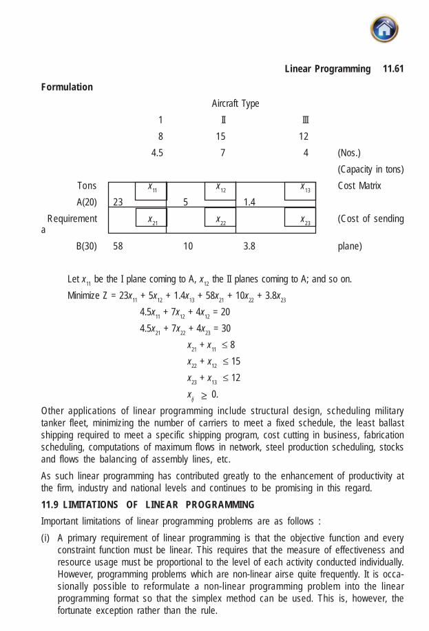
11.61Linear Programming
Formulation
Aircraft Type
1 II III
8 15 12
4.5 7 4 (Nos.)
(Capacity in tons)
Tons x11
x12
x13
Cost Matrix
A(20) 23 5 1.4
Requirement x21 x22 x23 (Cost of sendinga
B(30) 58 10 3.8 plane)
Let x11
be the I plane coming to A, x12
the II planes coming to A; and so on.
Minimize Z = 23x11 + 5x12 + 1.4x13 + 58x21 + 10x22 + 3.8x23
4.5x11
+ 7x12
+ 4x12
= 20
4.5x21 + 7x22 + 4x23 = 30
x21
+ x11
≤ 8
x22 + x12 ≤ 15
x23 + x13 ≤ 12
xij ≥ 0.
Other applications of linear programming include structural design, scheduling militarytanker fleet, minimizing the number of carriers to meet a fixed schedule, the least ballastshipping required to meet a specific shipping program, cost cutting in business, fabricationscheduling, computations of maximum flows in network, steel production scheduling, stocksand flows the balancing of assembly lines, etc.
As such linear programming has contributed greatly to the enhancement of productivity atthe firm, industry and national levels and continues to be promising in this regard.
11.9 LIMITATIONS OF LINEAR PROGRAMMING
Important limitations of linear programming problems are as follows :
(i) A primary requirement of linear programming is that the objective function and everyconstraint function must be linear. This requires that the measure of effectiveness andresource usage must be proportional to the level of each activity conducted individually.However, programming problems which are non-linear airse quite frequently. It is occa-sionally possible to reformulate a non-linear programming problem into the linearprogramming format so that the simplex method can be used. This is, however, thefortunate exception rather than the rule.

11.62 Advanced Management Accounting
(ii) It may not be possible to solve those problems using linear programming, in which non-linerarity arises because of joint interactions between some of the activities regardingthe total measure of effectiveness or total usage of some resource. Hence linear pro-gramming problem requires that the total measure of effectiveness and total resourceusage resulting from the joint performance of the activities must equal the respectivesums of these quantities resulting from each activity being performed individually.
In some situations, it may not be true. For example, consider a situation where by aproduct is produced with the scrap material from the primary product. The materialwould still have to be procured if only one of the two products were produced. However,the total material requirements if both products are produced is less than the sum ofrequirements is each were produced individually. It may not be possible to handle suchsituation with linear programming problems.
(iii) In linear programming problem, fractional values are permitted for the decisions vari-ables. However, many decision problems require that the solution for decision variableshould be obtained in non-fractional values. Rounding-off the values obtained by linearprogramming techniques may not result into an optimal solution in such cases.
(iv) In linear programming problem, coefficients in the objective function and the constraintequations must be completely known and they should not change during the period ofstudy i.e. they should be known constraints. In practical situation, it may not be possibleto state all coefficients in the objective function and constraints with certainity. Further-more, these coefficients may actually be random variables, each with an underlyingprobablility distribution for the values. Such problems cannot be solved using linearprogramming.
SUMMARYLinear Programming: The method of maximising (or minimising) a linear function ofseveral variables (called objective function) subject to the condition that the variables arenon negative and satisfy a set of linear equations and / or in equations (called linear constraints)hence called linear programming.
It involves three steps:
1. To identify the objective function as a linear function of its variables and state all thelimitation on resources as linear equation and / or in equations (constraints) – This iscalled a linear programming problem.
2. To use mathematical techniques to find all possible set or values of the variables(unknowns), satisfying the constraints. This is called a set of feasible solution.
3. To select the particular set of values of the variables obtained in step 2 above that leadto our objective pr maximum profit or least cost etc – This is called Optimum solutionof the Linear programming problem.

11.63Linear Programming
SELF-EXAMINATION QUESTIONS
1. The following is the production chart for a firm that produces both commercial use andscientific use calculators. The firm uses two departments in the assembling process.
Department D1
Department D2
Commercial-use 1 hour/unit 5 hours/unitScientific use 1 hour/unit 1 hour/unitAvailable hours 12 hours 12 hours
Profit for each unit of commercial use calculators is Rs. 30, and that for each unit of scien-tific use calculators is Rs. 60. Determine the number of calculators of each variety the firmshould produce in order to achieve the maximum profit. Also determine the maximum profit.
2. A tonic feed for cattle is to be prepared using two types of grain X1 and X2. Each unit of grainX1 weights 4 gms, and contain 2 gms of protein. Each unit of grain X2 weights 5 gms. andcontains 1 gm. of protein. The feed is to weight at most 40 gms. and must contain at least 10gms. of protein. If the grain X1 costs 30 paise a unit and that X2 costs 10 paise a unit,determine by graphical method the amount of two types of grain to be used in the prepara-tion of the feed to minimize the cost yet meeting the requirements. Also determine the mini-mum cost.
3. A manufacturer makes two products P1 and P2 using two machines M1 and M2. Product P1requires 2 hours on machine M1 and 6 hours on machine M2. Product P2 requires 5 hourson machine M1 and no time on machine M2. There are 16 hours of time per day availableon machine M1 and 30 hours on M2. Profit margin from P1 and P2 is Rs. 2 and Rs. 10 perunit respectively. What should be the daily production mix to optimise profit? Also determinethe maximum daily profit.
4. A firm manufactures two products A and B on which profits earned per unit are Rs. 3 and Rs.4 respectively. Each product is processed on two machines, M1 and M2. The product Arequires one minute of processing time on M1 and two minutes on M2 while B requires oneminute on M1 and one minute on M2. Machine M1 is available for use for not more than 7hours 30 minutes, while M2 is available for 10 hours during any working day. Find thenumber of units of products A2 and B to be manufactured to get the maximum profit.
5. A company produces two products X and Y, each of which requires processing in threemachines. The first machine can be used at most 70 hours; the second machine at most 40hours; and the third machine at most 90 hours. The product X requires 2 hours on machine1,1 hour on machine 2, and 1 hour on machine 3; the product Y requires 1 hour each onmachines 1 and 2, and 3 hours on the third machine. The profit is Rs. 50 per unitof X and Rs. 30 per unit of Y. How many units of each product should the companyproduce to maximize profit?
6. A carpenter has 90,80 and 50 running feet respectively of teak, plywood and rosewood. Theproduct A requires 2,1 and 1 running feet and the product B requires 1,2, and 1 running feetof teak, plywood and rosewood respectively. If A would sell for Rs. 48 and B for Rs. 40 perunit, how much of each should he make and sell in order to obtain maximum gross incomeout of his stock of wood?

11.64 Advanced Management Accounting
7. A machine producing either product A or B can produce A by using 2 units of chemicals and1 unit of a compound and can produce B by using 1 unit of chemicals and 2 units of thecompound. Only 800 units of chemicals and 1,000 units of the compound are available. Theprofits available per unit of A and B are respectively Rs. 30 and Rs. 20. Draw a suitablediagram to show the feasible region. Also, find the optimum allocation of units between A andB to maximize the total profit. Find the maximum profit.
8. A media specialist has decided on the allocation of advertisement in three media vehicles.Let x1 be the number of messages carried on the i-th media, i =1,2,3. the unit costs of amessage in the 3 media are Rs. 1000, Rs. 750 and Rs. 500. The total budget available is Rs.20,000 for the campaign period of a year. The first medium is a monthly magazine and it isdesired to advertise not more than one insertion in one issue. At least six messages shouldappear in the 2nd medium. The number of messages in the third medium should appear inbetween 4 and 8. The expected effective audience for unit message in the media vehicles isshown below:
Vehicle Expected effective audience1 80,0002 60,0003 45,000
It is desired to build the linear programming model to maximise the total effective audience.
9. A fertilizer company produces two types of fertilizer called grade I and II. Each of these typesis processed through two critical chemical plants. Plant A has maximum of 120 hours avail-able in a week and plant B has a maximum of 180 hours available. Manufacturing 1,000 kgof grade I fertilizer requires approximately 6 hours in Plant A and 4 hours in Plant B: manufac-turing 1,000 kg of grade II fertilizer requires 3 hours on plant A and 10 hours in plant B. Themaximum that the company can sell of grade I fertilizer is 18,000 kg. If profit is Rs. 450 per1,000 kg of grade I fertilizer and Rs. 550 per 1,000 kg of grade II fertilizer, it is required tobuild a mathematical model for amounts of the fertilizers that maximize the profit.
Also solve the problem graphically.(Answer : I = 13.75 units
I I = 12.50 unitsZ = Rs. 13062.50)
10. The Manager of Sohan Oil Co., wishes to find the optimal mix of two possible blendingprocesses. For process 1, an input of 1 unit of crude oil A and three units crude oil Bproduces an out put of 5 units of gasoline X and two units of gasoline Y. For process 2, aninput of 4 units of crude oil A and 2 unit of crude oil B produces an output of 3 units ofgasoline X and 8 units of gasoline Y. Let x1 and x2 be the number of units the companydecides to use of process 1 and process 2, respectively. The maximum amount of crude oilA available is 100 units and that of crude oil B is 150 units. Sales commitments require thatat least 200 units of gasoline X and 75 units of gasoline Y are produced. The unit profits ofprocess 1 and process 2 are p1 and p2 respectively. Formulate the blending problem as alinear programming model.

11.65Linear Programming
ANSWER TO SELF-EXAMINATION QUESTIONS
1. Commercial use calculator 0, Scientific use calculator 12; Max. profit = Rs. 720.
2. 5/3 units of X1 and 20/3 units of X2; Min. Cost = 350/3 paise
3. 0 unit of P1 and 3.2 unit of P2; Max Profit = Rs. 32.
4. 0 unit of A and 450 units of B.
5. 30 units of X and 10 units of Y.
6. 40 units of A and 10 units of B.
7. In figure 16, the shaded region is the feasible region.
Optimum allocation : 200 units of A and 400 units of B;
Max. Profit = Rs. 14,000.
8. Maximize Z = 80,000 x1 + 60,000 x2 + 45,000 x3
Subject to 1,000x1 + 750x2 + 500x3
≤ 20,000 (budget)
x1 ≤ 12
x2 ≥ 6
x3 ≥ 4
x3 ≤ 8
x1, x
2, ≥ 0
9. Let x1 be the amount in 1,000 kg. of grade I fertilizer produced and x2 the amount in 1,000 kgof grade II produced. The total profit
Z = 450 x1 + 550x
2 is to be maximized
subject to constraints 6x1 + 3x
2 ≤ 120 Plant A Capacity
2x1 + 10x
2 ≤ 180 Plant B Capacity
x1 ≤ 18
x1, x
2 ≥ 0.
10. Maximize Z = P1 x1 + P2 x2
Subject to x1 + 4x2 ≤ 100
3x1 + 2x2 ≤ 150
5x1 + 3x2 ≥ 200
2x1 + 8x2 ≥ 75
x1, x2 ≥ 0
(2 0 0 , 4 0 0 )(0 , 5 0 0 )
(4 0 0 , 3 0 0 )
(0 ,0 ) (4 0 0 ,0 )
2 x+
x=
80 0
12
x +x =
1
22
1 0 00
X 2
X�
(0 , 8 0 0 )
⎤⎥⎦
Availability
Demand⎤⎥⎦

12The Transportation Problem
LEARNING OBJECTIVES :
After studying this unit you will be able to :
� Formulate a transportation problem
� Find initial basic feasible solution by various methods
� Find minimum transportation cost schedule
� Ascertain minimum transportation cost schedule
� Discuss appropriate method to make unbalanced transportation problems balanced
� Examine prohibited and prefered routes
� Formulate and solve transportation problem
12.1 INTRODUCTION
This chapter is devoted to special problems that belong to the so called transportation class.These special problems are quite important from the practical point of view. Their practicalimportance arises because several real situations can be described by systems of equationsthat fall into the transportation class. Sizeable applications of linear programming problems havebeen made in this filed.
A typical transportation problem is concerned with selecting routes in a production distribution networkamong manufacturing plants and distribution warehouses or among regional distribution warehousesand local distribution outlets. The objective is to schedule transportation of products from sources todestination in such a way as to minimise the totak transportation cost.
A transportation problem can be paraphrased by considering m factories which supply to nwarehouses or distribution centers. The factories produce goods at level a
1, a
2,…am and the
demand are requirements of the distribution centers for these goods are b1, b
2….b
n respectively.
If the unit cost of shipping from i-th factory to warehouse j is cij what shipping pattern minimizes
the transportation cost?
Let xij denote number of units transported from factory I to destination j

12.2 Advanced Management Accounting
n
j=1∑ xij = ai, I = 1 ….m …………………..(1)
m
1=j∑ xij = b
jj = 1….n …………………(2)
Minimize Z = m n
i=j j=1∑ ∑ cij, x
ij…………………(3)
xij > 0 for all I,j
Equation 1 is interpreted as the sum of what leaves each factory (or origin) for the variouswarehouses (or destinations) is equal to what is produced at the factory, (2) implies that the sumof what arrives at each warehouse from the various origins in equal to the demand at thewarehouse. The double sum of equation 3 represents the total transportation cost. The non-negative conditions (4) arise because negative values for any x
ij have no physical meaning.
Solution to the problem described by equations 1 to 4 is given under the condition that
m n
i=j j=1i ja a=∑ ∑
From the physical point of view this condition means that the system of equations is in balancei.e., total production is equal to the total requirements. Equations (1) and (2) may be expandedas below.
X11 +x12…+x1n = a1
X12 +x22+ …+x2n= a2
Xm1+xm2+xmn = am
X11+x12+ ….+xm1 =b1
X12 +x22+ ….+xm2 = b2
:
:
:
X1n
+x2n
+ ….xmn
= bn
This is a system of (m+n) equations in mn unknown; but the equations are not independent. Twoimportant observations about the system of equations are worth noting.
i) The co-efficient of xij’s are either 1 or 0
ii) Any xij appears only once in the first m equations and once in the last n equations.
Our problem is to determine xij, the quantity that is to be shipped from the i-th origin to the j-thdestination in such a way that the total transportation cost is minimum. The quantities of interestcan be tabulated as below.

12.3The Transportation Problem
Destinations
Origins D1 D2… Di…. Da Available
01 c11 c12…. cij… c1n a1
02 c21 c22…. C2j… c2n a2
: : : : : :
0i c i1 ci12…. Cij…. cin ai
0m
cmi
cm2…. C
mj… c
mna
m
Required b1 b2… bj… bn Total
The method for solving the class of problems consist of finding a basic feasible solution. If it isnot optimal (an interactive procedure is used to improve it) then optimality test is applied to makeit an optimal solution.
12.2 METHODS OF FINDING INITIAL SOLUTION TO TRANSPORTATION PROBLEMS
12.2.1 Northwest corner Rule: The idea is to find an initial to find an initial basic feasiblesolution i.e., a set of allocations that satisfied the row and column totals. This method simplyconsists of making allocations to each row in turn, apportioning as much as possible to its firstcell and proceeding in this manner to its following cells until the row total in exhausted.
The algorithm involved under north-west corner rule consists for the following steps:
Steps:
1. Before allocation ensure that the total of availability and requirement is equal. If not thenmake same equal.
2. The first allocation is made in the cell occupying the upper left hand corner of the matrix.The assignment is made in such a way that either the resource availability is exhaustedor the demand at the first destination is satisfied.
3. (a) If the resource availability of the row one is exhausted first, we move down the secondrow and first column to make another allocation which either exhausts the resourceavailability of row two or satisfies the remaining destination demand of column one.
(b) If the first allocation completely satisfies the destination demand of column one, wemove to column two in row one, and make a second allocation which either exhausts theremaining resource availability of row one or satisfies the destination requirement undercolumn two.
4. The above procedure is repeated until all the row availability and column requirementsare satisfied. Consider, for example, the following sample problem. This method does notuse transportation costs which we shall bring in later in the other method.

12.4 Advanced Management Accounting
Row wise allocation as above, is made below. The maximum that can be allocated.
In cell (1, 1) 8 is allocated. This satisfies completely the requirements of column 1, butavailabilities of row 1 are not completely exhausted. Therefore, we proceed to cell (1,2) inrow 1 and allocate the remaining 2 units. We can start at cell (2,2) only since first column’srequirements have been completely satisfied, there is nothing that we can allocate in its firstcell (2,1). By the aforesaid procedure, we allocate 6 units to cell (2,2) and another 6 unitsto cell (2,3) exhausting completely the availabilities of row 2. This process is continueduntil we reach the cell (5,6).
12.2.2 The Least cost method:
i) Before starting the process of allocation ensure that the total of availability and demandis equal. The least cost method starts by making the first allocation in the cell whoseshipping cost (or transportation cost) per unit is lowest.
ii) This lowest cost cell is loaded or filled as much as possible in view of the origincapacity of its row and the destination requirements of its column.
iii) We move to the next lowest cost cell and make an allocation in view of the remainingcapacity and requirement of its row and column. In case there is a tie for the lowestcost cell during any allocation, we can exercise our judgment and we arbitrarilychoose cell for allocation.
iv) The above procedure is repeated till all row requirements are satisfied.
12.2.3 Vogel’s Approximation Method (VAM)
The Vogel’s Approximation Method (VAM) is considered to be superior to the northwestcorner rule in that it usually provides an initial solution that is optimal or nearly so. Therefore,we shall also stick to it for the discussion ahead. However, the readers may like to try theirhand on the following solved examples by the northwest corner rule and least-cost methodfor sake of practice. But we here apply VAM method.

12.5The Transportation Problem
VAM entails the following steps :
Step 1: For each row of the transportation table identify the smallest and next smallestcosts. Find the difference between the two costs and display it to the right of that row as“Difference” (Diff.). Likewise, find such a difference for each column and display it belowthat column. In case two cells contain the same least cost then the difference will be takenas zero.
Step 2: From amongst these row and column differences, select the one with the largestdifference. Allocate the maximum possible to the least cost cell in the selected column orrow. If there occurs a tie amongst the largest differences, the choice may be made for arow or column which has least cost. In case there is a tie in cost cell also, choice may bemade for a row or column by which maximum requirement is exhausted. Hatch that columnor row containing this cell whose totals have been exhausted so that this column or row isignored in further consideration.
Step 3: Recompute the column and row differences for the reduced transportation tableand go to step 2. Repeat the procedure until all the column and row totals are exhausted.
The VAM is applied to the previous problem on the table above as an illustration. Enteredin the table are the given unit shipping costs.
The arrow indicates that the last column having the largest difference from amongst allrows and columns is selected for allocation. Cell (2, 6) with the least cost is picked up and

12.6 Advanced Management Accounting
allocated 12 units. Row 2 is hatched since its total is exhausted.
This procedure is continued in the following tables until all the colums and rows are hatched.
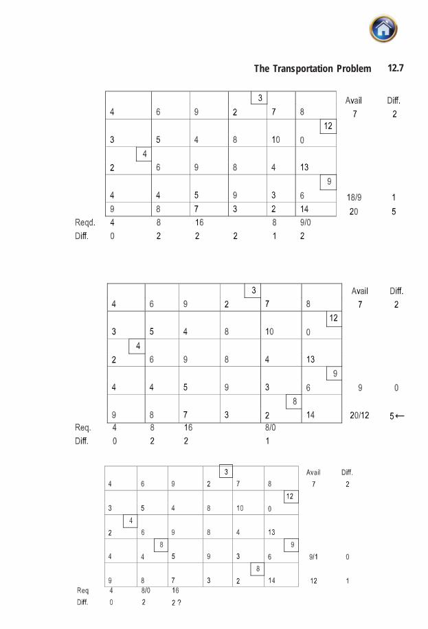
12.7The Transportation Problem
�

12.8 Advanced Management Accounting
Since only one column is left in the table above there is no question of finding the differencesand 16 units are allocated to the various cells of this column straightway as below
So many tables above have been drawn merely for exposition. All we shall see with thefollowing examples the initial allocation by VAM can as well be obtained in just one table.
The superiority of VAM lies in the fact that, unlike the Northwest Corner rule, not onlyavailabilities and requirements are taken into account but also due regard is paid to theunit costs. A row and column difference actually indicates the minimum unit penalty incurredby failing to make an allocation to the smallest cost cell in the row or column.
12.3 OPTIMALITY TEST:
Now we know how to obtain the initial basic feasible solution but it remains to be testedwhether it is optimal or not if it is not so, how do we go about deriving the optimal solution?Before we taken up this matter it is necessary to explain the concept of independence andnon-independence amongst allocations. Towards this, consider the following transportationtables of different problems. The allocations in these are shown by plus signs.

12.9The Transportation Problem
The lines constitute, in these allocation pattern what is known as loops. A loop may or maynot involve all the allocations. It consists of (at least 4) horizontal and vertical lines with anallocation at each corner which, in turn is a join of a horizontal and vertical line. At thisstage the last loop above is to be particularly noted. Here, two lines intersect each other atcell (2,4) and do not simply join; therefore, this is not to be regarded as a corner. Suchallocations in which a loop can be formed are known as non-independent, whereas thosein which a loop cannot be formed as regarded as independent. Towards explanation of thisnomenclature consider the following allocation pattern with a loop in it.
It is possible to progressively adjust the allocations along the corners of the loop withoutviolating the row and column totals. One adjusted allocations pattern for the above table isshow below as an example.

12.10 Advanced Management Accounting
But such a possibility of reallocation does not exist where a loop cannot be formed i.e.,allocations are independent.
Coming back now to the optimality test to be described shortly it can be applied to atransportation table if it satisfies the following conditions.
(1) it contains exactly m+n-1 allocations where m and n represent the number of rows andcolumn of the table.
(2) These allocations are independent i.e. a loop can not be performed by them
Without giving the proof, we may also mention that whenever there are m+n-1 allocationand a tick is placed in an empty cell one and only one loop can be passed through theticked cell and some are all of the m+n-1 allocation.
Cell Evaluations:
Consider the initial solution to the transportation problem on hand as obtained by VAM andreproduced above.
The allocations are m+n-1 in number and independent. It may be stated in passing thatinitial allocations obtained by Northwest Corner rule or VAM are always in independentpositions though they may be m+n-1 or less than m+n-1 in number. The motivation in theoptimality test is to see if it is possible to improve upon the existing solution. In the simplexlanguage, are any of the net evaluations negative? Before we attempt this for the problemon hand let us see what net evaluations mean in the context of transportation problems. Asin the simplex method, we want to replace a basic variable with a non-basic variable i.e.,want to zeroise an existing allocation cell and instead make some allocation in an emptycell. The problem then boils down to determination of an “outgoing allocation” and an“incoming allocation” that brings us closest to the optimal, if at all possible.

12.11The Transportation Problem
Towards this, we arbitrarily select the empty cell (1, 2), put a tick in it meaning that we wantto make some allocation in it and zeriosie one (or more) existing allocating. For reasonmentioned above, one and only one loop can be formed in the allocation pattern. It isshown in the table above. If we bring one unit to the ticket cell, other allocations on thecorners of the loop would be adjusted as below.
This would mean lowering of the cost by6×1-9×1+5×1-4×1 = 2This then is the net evaluation of the ticketed cell and obviously it would pay to bring thiscell into solution since the cost would be reduced by 2 per unit transferred to this along theloop. Likewise, we can compute cell evaluations for all the empty cells and select that asthe incoming one which has the most –ve cell evaluation.The procedure would consist of ticking each empty cell, forming a loop involving the tickand computing the cell evaluation for a unit transfer to the ticket cell along the loop. Obviouslythis would be a rather lengthy procedure. Fortunately there exists a much easier way ofcomputing cell evaluations for all empty cells at one stroke. This is what we described asthe optimality test above and it is applicable to transportation tables containing exactly m+m –1 independent allocations. It consists of the following steps:1. Determine a set of m +n numbers
ui ; i = 1, 2…m
vj ; j = 1, 2…n

12.12 Advanced Management Accounting
such that, for each occupied cell
cij = ui +vj
2. Compute the cell evaluation Δij for each empty cell (I, j) by the relationship
Δij = cij – (ui +vi)
Let us apply this optimality test to the problem on hand. Below is the table indicating just theunit costs in allocated cells in the problem on hand. We set u1 = 0 for row 1. it could beassigned any other value but zero has been assigned for ease in subsequent computations.
Also it is desirable to select that row or column which contains maximum number ofallocations. In this case row 1 has a maximum of 3 allocations. Now, we wish to find thevalue of v1, v3 and v4 for the column of these 3 allocations which can be accomplished asbelow.
U1 +v
1 = 4 Since u
1 = 0 therefore, v
i = 4
U1 +v
3 = 9 v
3 = 9
U1 +v
4 = 2 v
4 = 2
Values of v1 = 4, v
3 = 9, v
4 = 2 have been entered at the foot of each volume. Now let us
proceed with v1, v
3 and v
4 in turn.
v1: u
3 +v
1 = 2 since v
1 = 4, therefore, u
3 = -2 is entered
v3: u4 +v3 = 5 since v3 = 9, therefore, u4 = -4 is entered
v4: No more allocation in its column and we ignore it.
Having established and entered values of u2 and u4 let us take up these in turn.
u2: No more allocation in its row and we ignore it.
u4: u4 +v2 = 4 since u4 = -4 Therefore, v2 = 8 is entered
u4 +v6 = 6 since u4 = -4 therefore, v6 = 10 is entered
Proceeding is this manner we fill up all ui’s and vj’s
In the following table, we derive ui +v
j for each empty cell.

12.13The Transportation Problem
The following table gives te cell evaluations derived by subtracting above figures from theoriginal unit costs.
Since some of the Δijs are –ve the initial solution is not optimal. It would pay the most to
zeroise an existing allocation and allocate as much as possible to the most –ve Δij cell (6,
1). There are two cells having the same most –ve Δij. We pick up one of them arbitrarily for
ticking.
This is done below is the allocation table by ticking cell (1,6) and involving it in the only loop.
Transferring the maximum amount to the ticked cell
Reallocation is done by transferring the maximum amount to the ticketed cell. The rule forobtaining the maximum amount (say, θ max) that can be transferred to the ticked cell isderived below:
θ
θ θ

12.14 Advanced Management Accounting
Starting with the ticked cell θ is added to and subtracted from the corner allocationsalternately.
θ max = min of 3 - θ = 0
9 - θ = 0 = 3 Thus θ max = 3
Reallocation along this loop is shown below for clarity:
Complete reallocations follow:
The optimality test is performed below:

12.15The Transportation Problem
Since none of the Δij is –ve this solution is optimal.
Least cost 4×4 = 16
3×2 = 6
3×8 = 24
0×12 = 0
4×2 = 8
8×4 = 32
4×5 = 20
6×6 = 36
12×7 = 84
8×2 = 16
242 Answer
12.4 SPECIAL CASES
12.4.1 Unbalanced transportation problem
Illustration
A company has factories at A, B and C which supply warehouse at D, E, F and G. Monthlyfactory capacities are 160, 150 and 190 units respectively. Monthly warehouse requirementsare 80, 90, 110 and 160 units respectively. Units shipping costs (in Rs.) are as follows:
Solution
Availabilities = 160 +150 +190 = 500
Requirements = 80 +90 +110 +160 = 440
Availabilities –Requirement = 500 –440 = 60

12.16 Advanced Management Accounting
Therefore, a dummy warehouse H is introduced, and initial solution is obtained below byVAM in just one table.
12.4.2 Degeneracy : We know that a transportation problem has m +n –1 basic variableswhich means that the number of occupied cells is such a solution is one less than thenumber of rows plus the number of columns. It may happen sometimes that the number ofoccupied cells is less than m +n –1. Such a solution is called a degenerate solution. Wehandle such a situation by introducing an infinitesimally small allocation e in the least costand independent cell.
In this example, since there are only 6 (one less than m+n –1) allocations, an infinitesimallysmall allocation e is placed in the least cost and independent cell (1, 5). This solution istested for optimality below. (N.B.: if allocations we m +n –2 we would place two e’s, e1, e2which are virtually zero in the 2 least cost independent cells). This device enables us toapply to optimality test (m +n –1) allocations.
Δ

12.17The Transportation Problem
Since there are –ve Äij ‘s the initial solution is not optimal. Reallocation is donebelow by ticking the most -ve Äij cell (1, 3) and involving it in the loop.
√
√
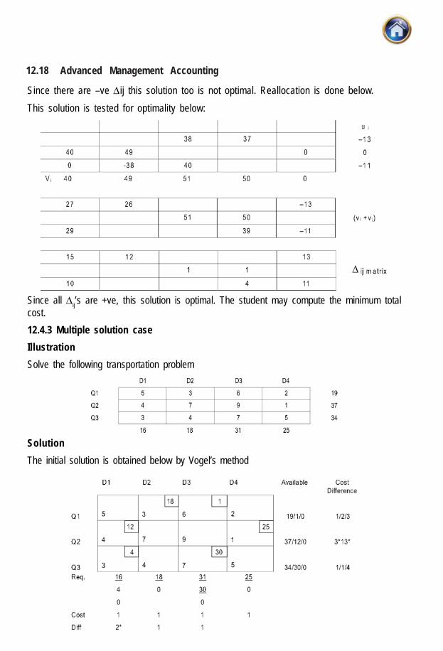
12.18 Advanced Management Accounting
Since there are –ve Δij this solution too is not optimal. Reallocation is done below.
This solution is tested for optimality below:
Since all Δij’s are +ve, this solution is optimal. The student may compute the minimum totalcost.
12.4.3 Multiple solution case
Illustration
Solve the following transportation problem
Solution
The initial solution is obtained below by Vogel’s method

12.19The Transportation Problem
Since there are 6 ( = m + n - 1) allocations the optimality test is performed below straightway:
Since all Δis ‘s are positive the initial solution itself is optimal. Also, since one Δij is zero thereexists other optimal solution, too i.e. A zero Δij for an unused square means that if this route werebrought into the solution, the shipping assignments would change, yet the total transportationcost would be same. To determine what this alternative optimal solution is, we follow the sameprocedure used for bringing any route into the solution.
12.5 MAXIMIZATION TRANSPORTATION PROBLEMS
Illustration
A company has 3 factories manufacturing the same product and 5 sole agencies in differentparts of the country. Production costs differ from factory to factory, and the sales prices fromagency to agency. The shipping cost per unit product from each factory to any agency isknown. Given the following data, find the production and distribution schedules mostprofitable to the company

12.20 Advanced Management Accounting
Solution
The profit matrix is derived below from the equation;
Profit = Sales –production cost –shipping cost.
The above profit matrix is converted into a loss matrix so that minimization transportation algo-rithms can be applied.
This is done by subtracting each entry of the above table from 14 (the largest number in thetable). Subsequently we get the following loss table.
Since the problem is unbalanced, a dummy warehouse is added and the initial solution isobtained by VAM below:
Since there are 8 ( = m + n - 1) allocations the optimality test is straightway performed below

12.21The Transportation Problem

12.22 Advanced Management Accounting
50×9 = 450
100×11 = 1,100
25×9 = 225
125×1 = 125
30×8 = 240
75×10 = 750
20×14 = __280
Rs. 3,170 Answer
12.6 PROHIBITED ROUTES:
Sometimes in a given transportation problem, some routes may not be available. Therecould be several reasons for this such as bad road conditions or strike etc. In such situations,there is a restriction on the route available for transportation. To handle such type of asituation, a very large cost (or a negative profit for the maximization problem) represented by∞ or M is assigned to each of such routes which are not available. Due to assignment ofvery large cost, such routes would automatically be eliminated in the final solution. Theproblem is the solved in its usual way.
Illustration
Solve the following transportation problem:
Note: It is not possible to transport any quantity from factory 2 to godown 5. State whetherthe solution derived by you is unique.
Solution
The initial solution is found by VAM below:

12.23The Transportation Problem
The above initial solution is tested for optimality. Since there are only 8 allocations and werequire 9(m+n-1 =9) allocations, we put a small quantity in the least cost independent cell(2, 6) and apply the optimality test. Let u
3 = 0 and then we calculate remaining ui and v
j
Now we calculate Δij = cij – (ui +vj) for non basic cells which are given in the table below:
Since all Δij are positive, the initial solution found by VAM is an optimal solution. The finalallocations are given below:
Factory to Godown Unit Cost Value
1 2 20 5 100
1 6 40 3 120
2 1 10 9 90
2 3 10 6 60
3 3 30 6 180
3 4 20 2 40
3 5 40 2 80
4 1 50 9 450
Total cost Rs. 1,120
The above solution is not unique because the opportunity cost of cell (1,2) is zero. Hencealternative solution exists. Students may find that the alternative solution is as given below:

12.24 Advanced Management Accounting
Factory to Godown Unit Cost Value
1 1 10 7 70
1 2 20 5 100
1 6 30 3 90
2 3 10 6 60
2 6 10 5 50
3 3 30 6 180
3 5 40 2 80
3 4 20 2 40
4 1 50 9 __450
Total cost (Rs.) 1,120
Illustration
The Link manufacturing company has several plants, three of which manufacture twoprincipal products, standard card table and deluxe card table. A new deluxe card table willbe introduced which must be considered in term of selling price & costs. The sellingprices are: Standard Rs. 14.95, Deluxe Rs. 18.95, and new Deluxe Rs. 21.95.
Requirements Variable costs Available plant capacity
Model Quantity Plant A Plant B Plant C Plant Capacity
Standard 450 8.00 7.95 8.10 A 800
Deluxe 1,050 8.50 8.60 8.45 B 600
New Deluxe 600 9.25 9.20 9.30 C 700
Solve this problem by the transportation technique for the greatest contribution.
Solution
(The student should be in a position to follow the computational steps below withoutexplanation)
6.95 7.00 6.85 Note: 6.95 = 14.95 – 8.00
10.45 10.35 10.50 10.45 = 18.95 – 8.50
12.70 12.75 12.65
Contribution matrix
The following relative loss matrix has been obtained by subtracting each figure in the abovecontribution matrix from the highest figure of 12.75 and multiplying by 100 to get wholenumbers for case in subsequent arithmetic.

12.25The Transportation Problem
The above allocation has been obtained by Vogel’s rule.
Since there are 4 i.e., less than m+ n-1 allocations, a small allocation e is placed in theleast cost independent cell (3, 1). The optimality test is performed below:
uj
580 580 575 575
230 225 225 (ui + vj) matrix
5 0 5 0
vi 0 –5 –5
0 15
15 Δij matrix
8
Since no Δij is –ve this initial solution itself is optimal. Also since there is one zero Δij thereexists alternate optimal solution too. The largest contribution is given by.
6.95×450 +10.45×350 +12.75×600 +10.50×700 =21,785 answer.
Note: in the examples solved herein we see that sometimes we get allocation less than m+n-1 in the initial solution. We place’s in the least cost independent cells. It is alsopossible that we get less than m +n –1 allocations in an intermediate reallocation in whichcase we would place e’s in the most –ve Δ
ij independent cell.
12.7 MISCELLANEOUS ILLUSTRATIONS
Illustration
A company wishes to determine an investment strategy for each of the next fouryears. Five investment types have been selected, investment capital has been allocated foreach of the coming four years, and maximum investment levels have been established foreach investment type. An assumption is that amounts invested in any year will remaininvested until the end of the planning horizon of four years. The following table summariesthe data for this problem. The values in the body of the table represent net return oninvestment of one rupee up to the end of the planning horizon. For example, a rupee

12.26 Advanced Management Accounting
invested in investment type B at the beginning of year 1 will grow to Rs. 1.90 by the end ofthe fourth year, yielding a net return of Rs. 0.90.
Investment made Investment Type Rs. Available
at the beginning (in ‘000)
of year
A B C D E
Net Return Data
1 0.80 0.90 0.60 0.75 1.00 500
2 0.55 0.65 0.40 0.60 0.50 600
3 0.30 0.25 0.30 0.50 0.20 750
4 0.15 0.12 0.25 0.35 0.10 800
Maximum
Rupee
investment (in ‘000) 750 600 500 800 1,000
The objective is this problem is to determine the amount to be invested at the beginning ofeach year in an investment type so as to maximize the net rupee return for the four-yearperiod. Solve the above transportation problem and get an optimal solution. Also calculatethe net return on investment for the planning horizon for four-year period.
Solution
We note that this transportation problem is an unbalanced one and it is a maximizationproblem. As a first step, we will balance this transportation problem.
Step 1:
Investment type
Years A B C D E Available Rs.(in ‘000)
NET RETURN DATA
1 0.80 0.90 0.60 0.75 1.00 500
2 0.55 0.65 0.40 0.60 0.50 600
3 0.30 0.25 0.30 0.50 0.20 750
4 0.15 0.12 0.25 0.35 0.10 800
Dummy 0 0 0 0 0 1000
Maximum 750 600 500 800 1,000 3,650
Rs. Investment
(in ‘000)

12.27The Transportation Problem
Step 2: We shall now convert the above transportation problem (a profit matrix) into a lossmatrix by subtracting all the elements from the highest value in the table viz. 1.00.
Investment type
Years A B C D E Available Rs.(in ‘000)
Net Loss Data (Rs.)
1 0.20 0.10 0.40 0.25 .0 500
2 0.45 0.35 0.60 0.40 0.50 600
3 0.70 0.75 0.70 0.50 0.80 750
4 0.85 0.88 0.75 0.65 0.90 800
Dummy 1.00 1.00 1.00 1.00 1.00 1,000
Maximum 750 600 500 800 1,000 3,650
Rs. Investment
(in ‘000)
For convenience, let us express the net loss data in the body of the above table inpaise. Thereafter, we shall apply VAM to get an initial solution.
Differences 25 25 20 15 50
25 40 10 10 30
15 – 5 15 10
15 – 25 35 10
15 – 25 – 10

12.28 Advanced Management Accounting
The initial solution got above by VAM is given below
We will now test the above solution for optimality.
Total number of allocations should be m +n –1 = 9 but there are only 8 allocations in theabove solution which are one less than 9, hence the initial solution found above isdegenerate. We introduce a small quantity e in an independent least cost cell which is (1,B) in this case to make the total number of allocation equal to 9. We introduce u
i’s and v
j’s
such that �ij =Cij –(ui +vj) (for i, j = 1, -5). We assume that u4 = 0 and various uj’s and vj’s and�ij’s are calculated as below. Values of various �ij’s are also written in the left hand cornerof the box for non basic cells.
����������� ����ij’s are negative, the above initial solution is not optimal. Introducing
in the cell (Dummy, B) with mos ����� �����ij an assignment e. The value of e and the new
solution as obtained from above is shown below. The values of ui’s, v
j’s are also calculated.
������ ���� ����� ������� ������ ����� ������������ ����ij =C
ij –(u
i +v
j) > 0 for
non allocated cells is also fulfilled.

12.29The Transportation Problem
������ ���� �ij’s are positive, hence, the second solution obtained above is optimal. Theallocation is given below.
In the year Investment type Amount (in ‘000)
1 E 500
2 B 600
3 D 750
4 A 250
4 C 500
4 D 50
The net return on investment for planning horizon of four years period is given by:
500×1.0+600 ×0.65 +750 ×0.50 +250 ×0.15 +500×0.25 +50×0.35 = Rs. 1,445 thousands
Illustration
XYZ and Co. has provided the following data seeking your advice on optimum investmentstrategy:
Investment made at Net return data (in paise) Amount
the beginning of year of selected investments available (lakhs)
P Q R S
1 95 80 70 60 70
2 75 65 60 50 40
3 70 45 50 40 90
4 60 40 40 30 30
Maximum Investment
(Lakhs) 40 50 60 60 —

12.30 Advanced Management Accounting
The following additional information are also provided:
— P, Q, R and S represents the selected investments.
— The company has decided to have four years investment plan.
— The policy of the company is that amount invested in any year will remain so until theend of the fourth year.
— The values (Paise) in the table represent net returns on investment of one Rupee tillthe end of the planning horizon (for example, a Rupee invested in investment P at thebeginning of year 1 will grow to Rs. 1.95 by the end of the fourth year, yielding a return of 95paise). Using the above, determine the optimum investment strategy.
SolutionThe given problem is an unbalanced transportation problem, which is converted into abalanced one by adding a dummy investment as given below:
Yeart Net return data (in paise) Amount
of investments available (lakhs)
P Q R S Dummy
1 95 80 70 60 0 70
2 75 65 60 50 0 40
3 70 45 50 40 0 90
4 60 40 40 30 0 30
Maximum Investment 40 50 60 60 20 —
The values in the table represent net return on investment of one rupee till the end of thefourth year. The objective of the company is to maximize the net return. For achieving thisobjective, let us convert this maximization problem into minimization problem by subtractingall the elements of the above payoff matrix from the highest payoff i.e. 95, and apply Vogel’sapproximation method for finding the initial feasible solution.

12.31The Transportation Problem
The solution obtained by VAM is as given below:
This initial solution is tested for optimality. There are 8 (=m +n-1) independent allocations.Let us introduce ui, vj, i = (1,2,3,4); j = (1, 2, 3, 4, 5) such that �ij = Cij –(ui +vj) for allocatedcells. We assume u1 = 0 and remaining uj’s, vj�� �����ij’s are calculated below.
On calculating� �ij’s for non-allocated cells, we found that their values are positive, hencethe initial solution obtained above is optimal. The optimal allocations are given below:
Year Invest in Net return
1 Invest Rs. 40 lakhs in investment P 0.95×Rs. 40 lakhs = Rs. 38,00,000
Rs. 30 lakhs in investment Q 0.80×Rs. 30 lakhs = Rs. 24,00,000
2 Invest Rs. 20 lakhs in investment Q 0.65×Rs. 20 lakhs = Rs. 13,00,000
Rs. 20 lakhs in investment R 0.60×Rs. 20 lakhs = Rs. 12,00,000
3. Invest Rs. 40 lakhs in investment R 0.50×Rs. 40 lakhs = Rs. 20,00,000
Rs. 50 lakhs in investment S 0.40×Rs. 50 lakhs = Rs. 20,00,000
4 Invest Rs. 10 lakhs in investment S 0.30×Rs. 10 lakhs = Rs. 3,00,000
Total Rs. 1,30,00,000
����������� ����ij ‘s = 0 the solution is not unique. Alternate solution exist.
Illustration
A particular product is manufactured in factories A, B, C, and D; and is sold at Centres 1, 2and 3. The cost in Rs. Of product per unit and capacity in kgms per unit time of each plantis given below:

12.32 Advanced Management Accounting
Factory Cost (Rs.) per unit Capacity (kgms) per unit
A 12 100
B 15 20
C 11 60
D 13 80
The sales price in Rs. Per unit and the demand in kgms per unit time are as follows:
Sales Centre Sales price (Rs.) per unit Demand (kgms) per unit
1 15 120
2 14 140
3 16 60
Find the optimal sales distribution.
Solution
The given problem is a transportation problem. The profit matrix for various factories andsales counters is calculated below:
Factory Sales Centres Capacity (kgms per unit
1 2 3
A 3 2 4 100
B 0 –1 1 20
C 4 3 5 60
D 2 1 3 80
Demand (kgms) 120 140 60
Since this is an unbalanced transportation problem (demand >capacity), let us introduce adummy factory with profit as Rs. 0 per until for various sales Centres and capacity equal tosixty units. The resulting matrix would be as below:
Factory Sales Centres Capacity (kgms per unit
1 2 3
A 3 2 4 100
B 0 –1 1 20
C 4 3 5 60
D 2 1 3 80
Dummy 0 0 0 60
Demand (kgms) 120 140 60

12.33The Transportation Problem
The above profit matrix can be converted into a loss matrix by subtracting all its elementsfrom the highest payoff of the matrix i.e. 5. The loss matrix so obtained is given below.
Factory Sales Centres Capacity (kgms per unit
1 2 3
A 2 3 1 100
B 5 6 4 20
C 1 2 0 60
D 3 4 2 80
Dummy 5 5 5 60
Demand (kgms) 120 140 60
The initial solution is obtained by applying Vogel’s approximation method.
The solution obtained by VAM is as given below:

12.34 Advanced Management Accounting
The initial solution is tested for optimality. The total number of independent allocations is6 which is one less than (m +n –1) allocations. Let us introduce a small quantity e in theleast cost independent cell (A, 3). We also introduce ui, vj, i = (1,2,3,4,5); j = (1,2,3) suchthat �ij =Cij – (ui +vj) for allocation cells.
We assume v2 = 0 and remaining vi’s, vj’s and �ij are calculated as below:
Since all �ij > 0 for the non allocated cells, hence the solution given by above matrix is optimal. The
optimal solution for the given problem is given below:
From Factory To sales Centre Quantity Profit per unit Total profit
(Rs.) (Rs.)
A 1 100 3 300
B 2 20 -1 -20
C 3 60 5 300
D 1 20 2 40
D 2 60 1 60
Dummy 2 60 0 0
Total profit 680
(Note: Since some of the �ij, are equal to zero, alternate solution also exists).
Illustraton
Factory Dstination
1 2 3 Supply to be exhausted
A 5 1 7 10
B 6 4 5 80
C 3 2 5 15
Demand 75 20 50

12.35The Transportation Problem
Since there is not enough supply, some of the demands at the three destinations may not besatisfied. For the unsatisfied demands, let the penalty costs be rupees 1,2 and 3 fordestinations (1), (2) and (3) respectively. Find the optimal allocation that minimises thetranportation and penalty cost.
Solution
Since demand (= 75+ 20 + 50 = 145) is greater than supply (= 10 + 80 +15 = 105) by 40 units,the given problem is an unbalanced one. We introduce a dummy factory with a supply of 40units. It is given that for the unsatisfied demands, the penalty cost is rupees 1,2 and 3 fordestinations (1), (2) and (3) respectively. Hence, the transportation problem becomes
The initial solution is obtained below by vogel’s method”

12.36 Advanced Management Accounting
The initial solution is given is the table below:
We now apply the optimality test to find whether the initial solution found above is optimal ornot.
The number of allocations is 6 which is equal to the required m +n –1 (=6) allocations.Also, these allocations are independent. Hence, both the conditions are satisfied.
Let us now introduce ui, and vj; i = (1,2,3,4) and j = (1,2,3) such that �ij = Cij –(ui +vi) forallocated cells. We assume that u2 =0 and remaining ui’s, v’j’s and �j’s are calculated.Since all �ij,’s for non basic cells are positive, therefore, the solution obtained above is anoptimal one. The allocation of factories to destinations and their cost is given below:-
Factor Destination units Cost Total cost
A 2 10 Re. 1 Rs. 10
B 1 20 Rs. 6 Rs. 120 Transportation
B 2 10 Rs. 4 Rs. 40 cost
B 3 10 Rs. 6 Rs. 40 Penalty cost
C 1 15 Rs. 3 Rs. 300
Dummy 1 40 Re. 1 Rs. 40
Rs. 555
Illustratoin
ABC enterprises is having three plants manufacturing dry-cells, located at different locations.Production cost differs from plant to plant. There are five sales offices of the companylocated in different regions of the country. The sales prices can differ from region to region.The shipping cost from each plant to each sales office and other data are given by followingtable:

12.37The Transportation Problem
Production cost per unit Production data table Plant No.
Maximum capacity in
No. of units
20 150 1
22 200 2
18 125 3
Shipping cost & demand & sales price table
Shipping cost
Sales office 1 Sales office 2 Sales office 3 Sales office 4 Sales office 5
Plant 1 1 1 5 9 4
Plant 2 9 7 8 3 6
Plant 3 4 5 3 2 7
Demand & sales prices
Sales office 1 Sales office 2 Sales office 3 Sales office 4 Sales office 5
Demand 80 100 75 45 125
Sales price 30 32 31 34 29
Find the production and distribution schedule most profitable to the company
Solution
The given information can be tabulated in following transportation problem:
Where entries in the cells of the above table indicate profit per unit received by selling one unitof item from plant i (1 =1,2,3) to the sales office (i=1,2,3,4,5). The profit per unit is calculatedusing the following formula.
Profit = Sales price –(Production cost +Shipping cost)
The objective of the company is to maximize the profit. For achieving this objective, let usconvert this maximization problem into minimization problem by subtracting all the elements ofthe above payoff matrix from the highest payoff i.e. Rs. 14.

12.38 Advanced Management Accounting
The problem is an unbalanced transportation problem since capacity (=475 units) is 50 unitsmore than the demand. Hence a dummy sales office is added with cost equal to zero for allplants and demand equal to 50 units. Now, let us apply Vogel’s Approximation method to theresultant balanced matrix for finding the initial feasible solution.
The initial solution obtained by VAM is given below which is tested for optimality.

12.39The Transportation Problem
These are m +n –1 =8 independent allocations. Let us now introduce ui, v
j, I = (1,2,3); j = (1,2—
—6) such that � ij = C
ij –(u
i +v
j) for allocation cells. We assume u
2 = 0 and remaining u
i’s v
j’s and
�ij’s are calculated as below:
������ ����� ����ij’s are negative, therefore, the above solution is not optimal. Introduce in
the cell (2,4) with ���� ����� �����ij�� ���������� �� �������������������������� ��
�� ������ ����������������������������������������� ����� ����������� � ��
���� ���������������� ����������i’s v
j ������
ij’s are again calculated.

12.40 Advanced Management Accounting
������ ���� �ij’s for non-basic cells are positive, therefore, the solution obtained above is an
optimal one. The allocation of plants to sales officers and their profit amount is given below:
Plant Sales units profit per profit
Office unit
1 1 50 9 450
1 2 100 11 1,100
2 4 25 9 225
2 5 125 1 125
2 Dummy 50 0 0
3 1 30 8 240
3 3 75 10 750
3 4 20 14 280
Total 3,170
SUMMARY
• Finding of initial base feasible solution
� North west corner method
� Least cost method
� Vogels approximation method
• Optimality test can be applied if it satisfies the given two conditions:
� It contains exactly m+n-1 allocations where m and n represent the number ofrows and column of the table.
� These allocations are independent i.e. a loop can not be performed by them.
SELF EXAMINATION QUESTIONS
1. Find the optimal solution of the following transportation problem :
D1
D2
D3
D4
Available
O1
23 27 16 18 30
O2 12 17 20 51 40
O3 22 28 12 32 53
Required 22 35 25 41 123
The cell entries are unit transportation costs.
(Answer : Opt. z = 2221).

12.41The Transportation Problem
Requirem
ents
2. Solve the following transportation problem :
D1 D2 D3 D4 D5 Available
O1 9 12 9 6 9 5
O2
7 3 7 7 5 4
O3
6 5 9 11 3 2
O4 6 8 11 2 2 9
Required 4 4 6 2 4 20
(Answer : Opt. z = 102).
3. Solve the following transportation problem :
Available
8 7 3 60
3 8 9 70
11 3 5 80
Required 50 80 80
(Answer : Opt. z = 75).
4. Solve the following transportation problem :
Stores1 2 3 4 5 6
1 9 12 9 6 9 10 5Factories 2 7 3 7 7 5 5 6
3 6 5 9 11 3 11 24 6 8 11 2 2 10 9
Availability 4 4 6 2 4 2

13The Assignment Problem
LEARNING OBJECTIVES :
After studying this unit, you will be able to :
� Use assignment technique, which is a special form of transportation problem.
� Use Hungarian Assignment Method.
� Negotiate with restrictions on assignments.
� Deal with unbalanced assignment problems.
� Prepare table with dummy rows and columns.
13.1 INTRODUCTION
The Assignement Problem is another special case of LPP. It occurs when n jobs are to beassigned to n facilities on a one-to-one basis with a view to optimising the resource required.
13.2 THE ASSIGNMENT ALGORITHM
The assingment problem can be solved by applying the following steps :
Step 1: Subtract the minimum element of each row from all the elements in that row. Fromeach column of the matrix so obtained, subtract its minimum element. The resulting matrixis the starting matrix for the following procedure.
Step 2: Draw the minimum number of horizontal and vertical lines that cover all the zeros.If this number of lines is n, order of the matrix, optimal assignment can be made by skippingsteps 3 and 4 and proceeding with step 5. If, however, this number is less than n, go to thenext step.
Step 3: Here, we try to increase the number of zeros in the matrix. We select the smallestelement out of these which do not lie on any line. Subtract this element from all such(uncovered) elements and add it to the elements which are placed at the intersections ofthe horizontal and vertical lines. Do not alter the elements through which only one linepasses.
Step 4: Repeat steps 1, 2 and 3 until we get the minimum number of lines equal to n.
Step 5 (A) Starting with first row, examine all rows of matrix in step 2 or 4 in turn until a rowcontaining exactly one zero is found. Surround this zero by , indication of an assignment

13.2 Advanced Management Accounting
there. Draw a vertical line through the column containing this zero. This eliminates anyconfusion of making any further assignments in that column. Process all the rows in thisway.
(B) Apply the same treatment to columns also. Starting with the first column, examine allcolumns until a column containing exactly one zero is found. Mark around this zero anddraw a horizontal line through the row containing this marked zero. Repeat steps 5A and B,until one of the following situations arises:
(i) No unmarked ( ) or uncovered (by a line) zero is left,
(ii) There may be more than one unmarked zero in one column or row. In this case, put around one of the unmarked zero arbitrarily and pass 2 lines in the cells of the remainingzeros in its row and column. Repeat the process until no unmarked zero is left in the matrix.
Illustration
An Accounts Officer has 4 suboridnates and 4 tasks. The subordinates differ in efficiency.The tasks also differ in their intrinsic difficulty. His estimates of the time each would take toperform each task is given in the matrix below. How should the tasks be allocated one toone man, so that the total man hours are minimized?
I II III IV
1 8 26 17 11
2 13 28 4 26
3 38 19 18 15
4 19 26 24 10
Let us apply the above steps take the above example.
Solution
Step 1
By subtracting the minimum element of each row from all its elements in turn, the givenmatrix reduces to
0 18 9 3
9 24 0 22
23 4 3 0
9 16 14 0
Next we subtract the minimum element of each column from all elements in turn, obtaining,
0 14 9 3
9 20 0 22
23 0 3 0
9 12 14 0

The Assignment Problem 13.3
Step 2
We draw the minimum number of lines to cover all zeros in the last matrix above as follows.To do so the first line is row 3 that contains the highest number of zeros. It can be seen that4( = n) lines cover all the zeros; hence optimal assignment is possible and it is obtained bythe application of step 5 straight away below.
0 14 9 3
9 20 0 22
23 0 3 0
9 12 14 0The optimal assignment, then is
1 → I, 2 → III, 3 → II, 4 → IV.
Minimum time taken = 8 + 4 + 19 + 10 = 41 hours.
Illustration
A manager has 5 jobs to be done. The following matrix shows the time taken by the j-th job(j = 1,2...5) on the i-th machine (i = 1,2,3...5). Assign 5 jobs to the 5 machines so that thetotal time taken is minimized.
Jobs1 2 3 4 5
I 9 3 4 2 10II 12 10 8 11 9III 11 2 9 0 8IV 8 0 10 2 1V 7 5 6 2 9
SolutionSubtracting the minimum element of each row from all its elements in turn, the givenmatrix reduces to
7 1 2 0 84 2 0 3 1
11 2 9 0 88 0 10 2 15 3 4 0 7
Now subtracting the minimum element of each column from its column, the matrixreduces to
3 1 2 0 70 2 0 3 07 2 9 0 7
4 0 10 2 0
1 3 4 0 6

13.4 Advanced Management Accounting
Next, we draw the minimum number of lines as follows:
3 1 2 0 7
0 2 0 3 0
7 2 9 0 7
4 0 10 2 0
1 3 4 0 6
Matrix A
Since there are only 3 lines (less than 5) optimal assignment cannot be made as yet. We,therefore, perform step 3 on the last matrix above. The minimum uncovered element is 1. Itis subtracted from all the uncovered elements and adding it to those at intersection of twolines, giving thereby the following matrix.
2 0 1 0 6
0 2 0 4 0
6 1 8 0 6
4 0 10 3 0
0 2 3 0 5
As can be seen below, minimum number of lines that cover all zeros is 5.
2 0 1 0 6
0 2 0 4 0
6 1 8 0 6
4 0 10 3 0
0 2 3 0 5
Optimal assignment is, therefore, possible and is made as per step 5 below:
2 0 1 0 6
0 2 0 4 0
6 1 8 0 6
4 0 10 3 0
0 2 3 0 5
Optimal assignment, then is
I → 2, II → 3, III → 4, IV → 5, V → 1.
Minimum time = 3 + 8 + 0 + 1 + 7 = 19.
Illustration
5 salesmen are to be assigned to 5 districts. Estimates of sales revenue in thousands ofrupees for each salesmen are given below.

The Assignment Problem 13.5
A B C D E
1 32 38 40 28 40
2 40 24 28 21 36
3 41 27 33 30 37
4 22 38 41 36 36
5 29 33 40 35 39
Find the assignment pattern that maximizes the sales revenue.
Solution
In order to convert this maximization problem into a minimization problem to be able toapply the assignment algorithm, we subtract each element from the highest, 41 and obtainthe following loss matrix.
9 3 1 13 1
1 17 13 20 5
0 14 8 11 4
19 3 0 5 5
12 8 1 6 2
Applying step 1 to the loss matrix we derive the following matrix, in which 4 lines are drawnto cover all zeros.
8 0 0 7 0
0 14 12 14 4
0 12 8 6 4
19 1 0 0 5
11 5 0 0 1
The minimum uncovered element is 4 that is subtracted from all elements and added to allelements at intersections. This yields the following matrix in which 5 lines are needed tocover all zeros.
12 0 0 7 0
0 10 8 10 0
0 8 4 2 0
23 1 0 0 5
15 5 0 0 1

13.6 Advanced Management Accounting
Step 5 (A) and (B) is applied below to obtain the optimal assignment.
12 0 0 7 0
0 10 8 10 0
0 8 4 2 0
23 1 0 0 5
15 5 0 0 1
Condition (ii) of Step B arises above; therefore cell (2,1) is arbitrarily chosen and putaround it and a line is also drawn in the second row.
12 0 0 7 0
0 10 8 10 0
0 8 4 2 0
23 1 0 0 5
15 5 0 0 1
This process is repeated below by putting around cell (3,4) arbitrarily chosen. Therefore,2 lines are drawn to cover 4th row and 3rd column.
12 0 0 7 0
0 10 8 10 0
0 8 4 2 0
23 1 0 0 5
15 5 0 0 1
The same process is continued to yield the optimal pattern as shown below:
12 0 0 7 0
0 10 8 10 0
0 8 4 2 0
23 1 0 0 5
15 5 0 0 1
Optimal assignment, then is
1 → B, 2 → A, 3 → E, 4 → C, and 5 → D.
The maximum assignment profit is given by Z = 38 + 40 + 37 + 41 + 35 = 191 thousandrupees.
13.2.1 Rationale of the Assignment Algorithm
Step 1: The relative cost of assigning facility i to job j is not changed by the subtraction ofa constant from either a column or a row of the original cost matrix.

The Assignment Problem 13.7
Step 2: An optimal assignment exists if total reduced cost of the assignment is zero. This isthe case when the minimum number of lines necessary to cover all zeros is equal to theorder of the matrix. If, however, it is less than n, a further reduction of the cost matrix has tobe undertaken.
Step 3: The underlying logic can be explained by means of Matrix A of Example 2, in whichonly 3( = n–2) lines can be drawn.
An optimal assignment is not possible. Further reduction is necessary. This reduction ismade by subtracting the smallest non-zero element from all elements in the matrix which is1.
This yields the following matrix:
2 0 1 –1 6
–1 1 –1 2 –1
6 1 8 –1 6
3 –1 9 1 –1
0 2 3 –1 5
This matrix contains -ve values. Since the objective is to obtain an assignment with thereduced costs of zero, the -ve numbers must be eliminated. This can be done by adding 1to each of the rows and columns crossed by 3 lines shown in matrix A of Example 2. Doingso in the above table yields the following matrix:
2 0 1 0 6
0 2 0 4 0
6 1 8 0 6
4 0 10 2 0
0 2 3 0 5
All this, in fact, amounts to step 3 i.e., add the least non-zero uncovered element to elementsat intersections, subtract it from all the uncovered elements and leave other elementsunaltered.
13.3 UNBALANCED ASSIGNMENT PROBLEMS
Like the unbalanced transportation problems there could arise unbalanced assignmentproblems too. They are to be handled exactly in the same manner i.e., by introducingdummy jobs or dummy men, etc. The following unbalanced problem serves as an example.
Illustration
To stimulate interest and provide an atmosphere for intellectual discussion, a finance facultyin a management school decides to hold special seminars on four contemporary topics–leasing, portfolio management, private mutual funds, swaps and options. Such seminarsshould be held once a week in the afternoons. However, scheduling these seminars (onefor each topic, and not more than one seminar per afternoon) has to be done carefully so

13.8 Advanced Management Accounting
that the number of students unable to attend is kept to a minimum. A careful study indicatesthat the number of students who cannot attend a particular seminar on a specific day is asfollows:
Leasing Portfolio Private Mutual Swaps and
Management Funds Options
Monday 50 40 60 20
Tuesday 40 30 40 30
Wednesday 60 20 30 20
Thursday 30 30 20 30
Friday 10 20 10 30
Find an optimal schedule of the seminars. Also find out the total number of students whowill be missing at least one seminar.
Solution
This is an unbalanced minimization assignment problem. We first of all balance it byadding a dummy topic:
Leasing Portfolio Private Swaps and Dummy
Management MutualFunds Options
Monday 50 40 60 20 0
Tuesday 40 30 40 30 0
Wednesday 60 20 30 20 0
Thursday 30 30 20 30 0
Friday 10 20 10 30 0
Subtracting the minimum element of each column from all the elements of that column,we get the following matrix :
Leasing Portfolio Private Swaps and Dummy
Management Mutual Funds Options
Monday 40 20 50 0 0
Tuesday 30 10 30 10 0
Wednesday 50 0 20 0 0
Thursday 20 10 10 10 0
Friday 0 0 0 10 0
The minimum number of lines to cover all zeros is 4 which is less than the order of thesquare matrix, (i.e. 5), the above matrix will not give the optimal solution. Subtract the

The Assignment Problem 13.9
minimum uncovered element (=10) from all uncovered elements and add it to the elementslying on the intersection of two lines, we get the following matrix:
Leasing Portfolio Private Swaps and Dummy
Management Mutual Funds Options
Monday 30 20 40 0 0
Tuesday 20 10 20 10 0
Wednesday 40 0 10 0 0
Thursday 10 10 0 10 0
Friday 0 10 0 20 10
Since the minimum number of lines to cover all zeros is 5 which is equal to the order of thematrix, the above matrix will give the optimal solution which is given below:
Leasing Portfolio Private Swaps and Dummy
Management Mutual Funds Options
Monday 30 20 40 0 0
Tuesday 20 10 20 10 0
Wednesday 40 0 10 0 0
Thursday 10 10 0 10 0
Friday 0 10 0 20 10
and the optimal schedule is
No. of students missing
Monday: Swaps and options 20
Tuesday: No seminar 0
Wednesday: Portfolio Management 20
Thursday: Pvt. Mutual funds 20
Friday: Leasing 10
70
Thus, the total number of students who will be missing at least one seminar = 70
Illustration
A solicitor's firm employs typists on hourly piece-rate basis for their daily work. There arefive typists for service and their charges and speeds are different. According to an earlierunderstanding only one job is given to one typist and the typist is paid for full hours even ifhe works for a fraction of an hour. Find the least cost allocation for the following data:

13.10 Advanced Management Accounting
Typist Rate per hour No. of pagesJob No. of pages
(Rs.) typed/hour
A 5 12 P 199
B 6 14 Q 175
C 3 8 R 145
D 4 10 S 198
E 4 11 T 178
Solution
The following matrix gives the cost incurred if the ith typist (i = A, B, C, D, E) executes the jthjob (j = P, Q, R, S, T):
Job
Typist P Q R S T
A 85 75 65 125 75
B 90 78 66 132 78
C 75 66 57 114 69
D 80 72 60 120 72
E 76 64 56 112 68
Subtracting the minimum element of each row from all its elements in turn, the abovematrix reduces to
Job
Typist P Q R S T
A 20 10 0 60 10
B 24 12 0 66 12
C 18 9 0 57 12
D 20 12 0 60 12
E 20 8 0 56 12
Now subtract the minimum element of each column from all its elements in turn, the abovematrix reduces to
2 2 0 4 0
6 4 0 10 2
0 1 0 1 2
2 4 0 4 2
2 0 0 0 2

The Assignment Problem 13.11
Since there are only 4 lines (< 5) to cover all zeros, optimal assignment cannot be made.The minimum uncovered element is 2.
We subtract the value 2 from all uncovered elements, add this value to all junction valuesand leave the other elements undisturbed. The revised matrix looks as:
2 2 2 4 0
4 2 0 8 0
0 1 2 1 2
0 2 0 2 0
2 0 2 0 2
Since the minimum number of lines required to cover all the zeros is only 4 (< 5), optimalassignment cannot be made at this stage also.
The minimum uncovered element is 1. Repeating the usual process again, we get thefollowing matrix:
2 1 2 3 0
4 1 0 7 0
0 0 2 0 2
0 1 0 1 0
3 0 3 0 3
Since the minimum number of lines to cover all zeros is equal to 5, this matrix will giveoptimal solution. The optimal assignment is made in the matrix below:
Typist/Job P Q R S T
A 2 1 2 3 0
B 4 1 0 7 0
C 8 0 2 0 2
D 0 1 0 1 0
E 3 0 3 0 3
Cost (Rs.)
Thus typist A is given job T : 75
Typist B is given job R : 66
Typist C is given job Q : 66
Typist D is given job P : 80
Typist E is given job S : 112
Total Rs. 399
Note: In this case the above solution is not unique. Alternative solution also exists.

13.12 Advanced Management Accounting
Illustration
WELLDONE Company has taken the third floor of a multi-storeyed building for rent with aview to locate one of their zonal offices. There are five main rooms in this floor to beassigned to five managers. Each room has its own advantages and disadvantages. Somehave windows, some are closer to the washrooms or to the canteen or secretarial pool.The rooms are of all different sizes and shapes. Each of the five managers was asked torank their room preferences amongst the rooms 301, 302, 303,304 and 305. Theirpreferences were recorded in a table as indicated below:
MANAGERM1 M2 M3 M4 M5
302 302 303 302 301303 304 301 305 302304 305 304 304 304
301 305 303302
Most of the managers did not list all the five rooms since they were not satisfied with someof these rooms and they have left off these from the list. Assuming that their preferencescan be quantified by numbers, find out as to which manager should be assigned to whichroom so that their total preference ranking is a minimum.
Solution
Let us first formulate the preference ranking assignment problem.
MANAGERS
Room No. M1 M2 M3 M4 M5
301 – 4 2 – 1302 1 1 5 1 2303 2 – 1 4 –304 3 2 3 3 3305 – 3 4 2 –
We have to find an assignment so that total preference ranking is minimum. In a cell (-)indicates that no assignment is to be made in that particular cell. Let us assign a very largeranking value M to all such cells.
Step 1 : From each row, subtract the minimum element of that row, from all the elementsof that row to get the following matrix.
MANAGERSRoom No M1 M2 M3 M4 M5
301 M 3 1 M 0302 0 0 4 0 1303 1 M 0 3 M304 1 0 1 1 1305 M 1 2 0 M

The Assignment Problem 13.13
Draw the minimum number of lines in the above table to cover all zeros. In this case thenumber of such lines is five, so the above matrix will give the optimal solution. Theassignment is made as below:
MANAGERS
Rooms No. M1 M2 M3 M4 M5
301 M 3 1 M 0
302 0 0 4 0 1
303 1 M 0 3 M
304 1 0 1 1 l
305 M 1 2 0 M
Thus, the assignment is
M1 → 302, M2 → 304, M3 → 303, M4 → 305, M5 → 301
and the total minimum ranking = 1 + 2 + 1 + 2 + 1 = 7
Illustration
XYZ airline operating 7 days a week has given the following timetable. Crews must have aminimum layover of 5 hours between flights. Obtain the pairing flights that minimizes layovertime away from home. For any given pairing the crew will be based at the city that results inthe smaller layover.
Chennai-Mumbai Mumbai-Chennai
Flight Number Depart. Arrive Flight Number Depart. ArriveA1 6 AM 8 AM B1 8 AM 10 AMA2 8 AM 10 AM B2 9 AM 11 AMA3 2 PM 4 PM B3 2 PM 4 PMA4 8 PM 10 PM B4 7 PM 9 PM
Solution
To begin with, let us first assume that the crew is based at Chennai. The flight A1, whichstarts from Chennai at 6 AM, reaches Mumbai at 8 AM. The schedule time for the flight atMumbai is 8 AM. Since the minimum layover time for crew is 5 hours, this flight can departonly on the next day i.e. the layover time will be 24 hours. Similarly, layover times for otherflights are also calculated and given in the following table.
Crew based at Chennai
Flight No. B1 B2 B3 B4
A1 24 25 6 11A2 22 23 28 9A3 16 17 22 27A4 10 11 16 21

13.14 Advanced Management Accounting
The layover times for various flight connections when crew is assumed to be based atMumbai are similarly calculated in the following table.
Crew based at Mumbai
Flight No. B1 B2 B3 B4
A1 20 19 14 9
A2 22 21 16 11
A3 28 27 22 17
A4 10 9 28 23
Now since the crew can be based at either of the places, minimum layover times can beobtained for different flight numbers by selecting the corresponding lower value out of theabove two tables. The resulting table is as given below:
Flight No.
Flight No. B1 B2 B3 B4
A1 20* 19* 6 9 *
A2 22 21* 16* 9
A3 16 17 22 17*
A4 10 9 * 16 21
A * with an entry in the above table indicates that it corresponds to layover time when thecrew is based at Mumbai. We will now apply the assignment algorithm to find the optimalsolution. Subtracting the minimum element of each row from all the elements of that row,we get the following matrix.
Flight No.
Flight No. B1 B2 B3 B4
A1 14 13 0 3
A2 13 12 7 0
A3 0 1 6 1
A4 1 0 7 12
Since there is a zero in each column, there is no need to perform column reduction. Theminimum number of lines to cover all zeros is four which is equal to the order of the matrix.Hence, the above table will give the optimal solution. The assignment is made below:
Flight No.
Flight No. B1 B2 B3 B4
A1 14 13 0 3
A2 13 12 7 0
A3 0 1 6 1
A4 1 0 7 12

The Assignment Problem 13.15
The optimal assignment is
From flight No. To flight No. Layover time
A1 B3 6
A2 B4 9
A3 B1 16
A4 B2* 9
40 hours
Illustration
An organisation producing 4 different products viz. A,B, C and D having 4 operators viz.P,Q,R and S, who are capable of producing any of the four products, works effectively 7hours a day. The time (in minutes) required for each operator for producing each of theproduct are given in the cells of the following matrix along with profit (Rs. per unit).
Operator Product
A B C D
P 6 10 14 12
Q 7 5 3 4
R 6 7 10 10
S 20 10 15 15
Profit (Rs./Unit) 3 2 4 1
Find out the assignment of operators to products which will maximize the profit.
Solution
Using the information that the factory works effectively 7 hours (= 420 minutes) a day, andthe time required by each operator for producing each of the products, we obtain thefollowing production and profit matrices.
In order to apply assignment algorithm for minimizing losses, let us first convert this profitmatrix to a loss matrix by subtracting all the elements of the given matrix from its highestelement which is equal to Rs. 560. The matrix so obtained is given below:
Production Matrix (units)Operator Product
A B C D
P 70 42 30 35
Q 60 84 140 105
R 70 60 42 42
S 21 42 28 28
Profit Matrix (in Rs.)Operator Product
A B C D
P 210 84 120 35
Q 180 168 560 105
R 210 120 168 42
S 63 84 112 28

13.16 Advanced Management Accounting
Now apply the assignment algorithm to the above loss matrix. Subtracting the minimumelement of each row from all elements of that row, we get the following matrix:
Now subtract the minimum element of each column from all the elements of that column toget the following matrix:
Draw the minimum number of lines to cover all zeros. The minimum number of lines tocover all zeros is three which is less than the order of the square matrix (i.e. 4), thus theabove matrix will not give the optimal solution. Subtract the minimum uncovered element (=62) from all uncovered elements and add it to the elements lying on the intersection of twolines, we get the following matrix:
Operator ProductA B C D
P 350 476 440 525
Q 380 392 0 455
R 350 440 392 518
S 497 476 448 532
Operator ProductA B C D
P 0 126 90 175Q 380 392 0 455R 0 90 42 168S 49 28 0 84
Operator ProductA B C D
P 0 98 90 91Q 380 364 0 371R 0 62 42 84S 49 0 0 0
Operator ProductA B C D
P 0 36 90 29Q 380 302 0 309R 0 0 42 22S 111 0 62 0

The Assignment Problem 13.17
The minimum number of lines which cover all zeros is 4 which is equal to the order of thematrix, hence, the above matrix will give the optimal solution. Specific assignments in thiscase are as shown below:
Illustration
A firm produces four products. There are four operators who are capable of producing anyof these four products. The processing time varies from operator to operator. The firmrecords 8 hours a day and allow 30 minutes for lunch. The processing time in minutes andthe profit for each of the products are given below:
Operators Products
A B C D
1 15 9 10 6
2 10 6 9 6
3 25 15 15 9
4 15 9 10 10
Profit (Rs.) per unit 8 6 5 4
Find the optimal assignment of products to operators.
Solution
The firm records 8 hours a day and allows 30 minutes for lunch, hence the net workingtime available per day is 7 hours and 30 minutes i.e. 450 minutes. The number of units ofeach product which could be produced in 450 minutes by the four operators is calculatedin the table given below:
Operator ProductA B C D
P 0 36 90 29Q 380 302 0 309R 0 0 42 22S 111 0 62 0
Operator Product Profit (Rs.)P A 210Q C 560R B 120S D 28
Total Profit (Rs.) 918

13.18 Advanced Management Accounting
Operators Products
A B C D
1 30 50 45 75
2 45 75 50 75
3 18 30 30 50
4 30 50 45 45
Profit (Rs.) per unit 8 6 5 4
Since we are given the profit per unit of each product, the profit matrix is computed as givenbelow:
Operators Profits Matrix in Rs. of Products
A B C D
1 240 300 225 300
2 360 450 250 300
3 144 180 150 200
4 240 300 225 180
The above profit matrix is converted into a loss matrix by subtracting all the elements of theprofit matrix from its highest pay off Rs. 450. The loss matrix so obtained is given below:
Operators Loss matrix – Products
A B C D
1 210 150 225 150
2 90 0 200 150
3 306 270 300 250
4 210 150 225 270
Let us now apply the assignment algorithm that is 'Hungarian Rule' to the above loss matrix.Accordingly, subtract the minimum element of each row from all its elements in turn, theabove matrix thus reduces to
Operators Loss matrix – Products
A B C D
1 60 0 75 0
2 90 0 200 150
3 56 20 50 0
4 60 0 75 120
Subtract the minimum element of each column from all the elements of the column inturn. Draw the minimum number of lines in the resultant matrix so as to cover all zeros, weget

The Assignment Problem 13.19
Operators Loss matrix - Products
A B C D
1 4 0 25 0
2 34 0 150 150
3 0 20 0 0
4 4 0 25 120
Since the minimum number of lines to cover all zeros is three which is one less than theorder of the matrix, we subtract the minimum uncovered element (= 4) from all uncoveredelements and add it to the elements lying at the intersection of two lines. The matrix soobtained is given below:
Operators Loss matrix - Products
A B C D
1 0 0 21 0
2 30 0 146 150
3 0 24 0 4
4 0 0 21 120
Since the minimum number of lines to cover all zeros is 4 which is equal to the order of thematrix, the above matrix will give optimal solution. The optimal assignments are givenbelow:
Operators Loss matrix - Products
A B C D
1 0 0 21 0
2 30 0 146 150
3 0 24 0 4
4 0 0 21 120
The optimal assignment is as shown below:
Operators Products Profit (Rs.)
1 D 300
2 B 450
3 C 150
4 A 240
Rs. 1140

13.20 Advanced Management Accounting
Illustration
A manufacturing company, four has zones A, B, C, D and four sales engineers P, Q, R, Srespectively for assignment. Since the zones are not equally rich in sales potential, thereforeit is estimated that a particular engineer operating in a particular zone will bring the followingsales:
Zone A : 4,20,000
Zone B : 3,36,000
Zone C : 2,94,000
Zone D : 4,62,000
The engineers are having different sales ability. Working under the same conditions, their yearlysales are proportional to 14, 9, 11 and 8 respectively. The criteria of maximum expected totalsales is to be met by assigning the best engineer to the richest zone, the next best to the secondrichest zone and so on.
Find the optimum assignment and the maximum sales.
Solution
It is given that the yearly sales of four sales engineers are proportional to 14, 9, 11 and 8respectively. The sum of proportions is 14+9+11+8=42.
Let us assume that Rs. 1,000 is equivalent to one unit. The sales units of four engineers in fourdifferent zones have been calculated as in the following table :
Sales Zones
Engineer A B C D
P (14/42)×420 (14/42)×336 (14/42)×294 (14/42)×462
= 140 = 112 = 98 = 154
Q (9/42)×420 (9/42)×336 (9/42)×294 (9/42)×462
= 90 = 72 = 63 = 99
R (11/42)×420 (11/42)×336 (11/42)×294 (11/42)×462
= 110 = 88 = 77 = 121
S (8/42)×420 (8/42)×336 (8/42)×294 (8/42)×462
= 80 = 64 = 56 = 88
The problem here is to find the optimum assigment in the following sales table so as tomaximise the total sales of the company.
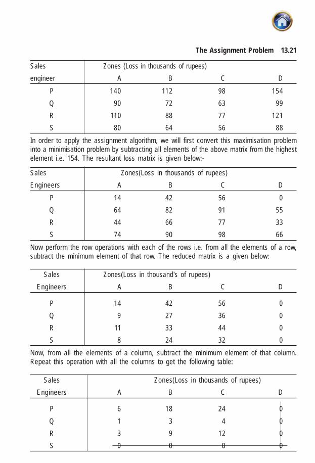
The Assignment Problem 13.21
Sales Zones (Loss in thousands of rupees)
engineer A B C D
P 140 112 98 154
Q 90 72 63 99
R 110 88 77 121
S 80 64 56 88
In order to apply the assignment algorithm, we will first convert this maximisation probleminto a minimisation problem by subtracting all elements of the above matrix from the highestelement i.e. 154. The resultant loss matrix is given below:-
Sales Zones(Loss in thousands of rupees)
Engineers A B C D
P 14 42 56 0
Q 64 82 91 55
R 44 66 77 33
S 74 90 98 66
Now perform the row operations with each of the rows i.e. from all the elements of a row,subtract the minimum element of that row. The reduced matrix is a given below:
Sales Zones(Loss in thousand's of rupees)
Engineers A B C D
P 14 42 56 0
Q 9 27 36 0
R 11 33 44 0
S 8 24 32 0
Now, from all the elements of a column, subtract the minimum element of that column.Repeat this operation with all the columns to get the following table:
Sales Zones(Loss in thousands of rupees)
Engineers A B C D
P 6 18 24 0
Q 1 3 4 0
R 3 9 12 0
S 0 0 0 0

13.22 Advanced Management Accounting
The minimum number of lines drawn to cover all zeros is 2 which is less than the order ofthe matrix (i.e.4), hence we can not make assignments. Subtract the minimum uncoveredelement from all the uncovered elements and add it to the elements lying at the intersectionof two lines, we get:
Sales Zones (Loss in thousand of rupees)
Engineers A B C D
P 5 17 23 0
Q 0 2 3 0
R 2 8 11 0
S 0 0 0 0
The minimum number of lines drawn again to cover all the zeros is 3 which is one lessthan the order of the matrix. Repeat the above step which gives the following table:
Sales Zones (Losss in thousands of rupees)
Engineers A B C D
P 5 15 21 0
Q 0 0 1 0
R 2 6 9 0
S 2 0 0 3
The minimum number of lines to cover all zeros is still one less than the order of the matrix.Repeat the above step again, which gives the following table:
Sales Zones (Loss in thousands of rupees)
Engineers A B C D
P 3 13 19 0
Q 0 0 1 2
R 0 4 7 0
S 2 0 0 5

The Assignment Problem 13.23
The minimum number of lines drawn to cover all the zeros is 4 which is equal to the orderof the matrix. Hence, the above table will give the optimum assignment. The assignmentsare as follows:
Sales Zones (Loss in thousands of rupees
Engineers A B C D
P 3 13 19 0
Q 0 0 1 2
R 0 4 7 0
S 2 0 0 5
Engineers Zones Sales (in Rs.)
P D 1,54,000
Q B 72,000
R A 1,10,000
S C 56,000
3,92,000
It can be seen from the above assignments that the best engineer P is assigned to therichest zone D, the next best engineer R is assigned to second richest zone A, the next bestengineer Q is assigned to zone B and so on. Hence, the optimum assignment matches thecompany's criteria of achieving the maximum expected total sales.
SELF EXAMINATION QUESTIONS
1. Solve the following assignment problems:
(a)
Jobs
Men 1 2 3 4 5
1 2 9 3 7 1
2 6 8 7 6 1
3 4 6 5 3 1
4 4 2 7 3 1
5 5 3 9 5 1

13.24 Advanced Management Accounting
(b)
8 4 2 7 10 9 5 5 43 8 9 2 64 3 1 0 39 5 8 9 5
(c)Jobs
Men 1 2 3 4 5 61 5 0 6 8 7 42 5 2 3 0 6 73 3 4 4 3 5 24 3 9 7 2 7 65 9 8 7 8 4 56 1 8 7 4 2 3
2. A company has 4 machines on which to do 3 jobs. Each job can be assigned to one andonly one machine. The cost of each machine is given in the following table:
Jobs MachineW X Y Z
A 18 24 28 32B 8 13 17 19C 10 15 19 22
What are the job assignments which will minimize the cost ?(Answer: A/W, B/X, C/Y)3. A management consulting firm has a backlog of 4 contracts. Work on these contractsmust be started immediately. Three project leaders are available for assignment to thecontracts. Because of the varying work experience of the project leaders, the profit toconsulting firm will vary based on the assignment as shown below. The unassigned contractcan be completed by subcontracting the work to an outside consultant. The profit on thesubcontract is zero.
Project ContractLeader 1 2 3 4A 13 10 9 11B 15 17 13 20C 6 8 11 7Dummy 0 0 0 0
Find the optimal assignment. Note that the problem is basically not only unbalanced (thoughnow balanced by inclusion of dummy) but also a maximization one.Answer: A → 1, B → 4, C → 3, Dummy → 2

14.1Critical Path Analysis
14Critical Path Analysis
LEARNING OBJECTIVES :
After studying this unit you will be able to :
� Explain the generic term network analysis
� Draw diagram & chart representing inter-relationships between various elementsof the project and finally establishing critical path
� Identify Dummy Activities
� Identify earliest and latest event times of each event. Identify different types of FloatHelp in Decision Making about project times and resource allocation Calculatingprobability of completing network in a given time
14.1 INTRODUCTION
Planning, Scheduling and Controlling are three important functions of management. Plan-ning involves the formulation of objectives and goals that are subsequently translated intospecific plans and projects. Scheduling is concerned about the implemention of activitiesnecessary to achieve the laid down plans. The function of control is to institute a mecha-nism that can trigger a warning signal if actual performance is deviating (in terms of time,cost and some other measures of effectiveness) from the plan. If such a deviation is unac-ceptable to the concerned manager, he will be required to take corrective action to bringperformance in conformity with the plans. The PERT and CPM models are extremely usefulfor the purpose of planning, scheduling and controlling the progress and completion oflarge and complex projects or for carrying out the analysis of these three managerial func-tions. Before we describe the basic concepts used in the construction and analysis of thesemodels, let us first understand the meaning of a project.
What is a project?
A project can be defined as a set of large number of activities or jobs that are performed ina certain sequence determined logically or technologically and it has to be completedwithin (i) a specified time, (ii) a specified cost and (iii) meeting the performance standards.Examples of a project from fairly diverse fields are given below:
1. Introducing a new product in the market.
2. Construction of a new bridge over a river or construction of a 25 storied building.

14.2 Advanced Management Accounting
3. Executing a large and complex order on jobbing production.
4. Sending a spacecraft to the mars.
14.2 GENERAL FRAMEWORK OF PERT/CPM
A network is a graphical representation of a project, depicting the flow as well as thesequence of well-defined activities and events. Developed during the 1950s, both CPM(Critical Path Method) and PERT (Programme Evaluation and Review Technique) arenetwork tehcniques/models. The network approach helps project managers in planning,scheduling and controlling. As a planning tool it helps the manager to estimate the require-ments of resources viz., materials, equipment, manpower, cost and time for each activity ortasks of the project. This approach cannot make decisions by its own. It only providesadditional information to executives to facilitate decision making process. Also it does notprovide solution to every management problem. It certainly helps in identification of thoseactivities, jobs or events which control the completion of the project.
The working methodology of critical path analysis (CPA) which includes both CPM andPERT, consists of following five steps:
1. Analyse and break down the project in terms of specific activities and/ or events.
2. Determine the interdependence and sequence of specific activities and prepare a net-work.
3. Assign estimates of time, cost or both to all the activities of the network.
4. Identify the longest or critical path through the network.
5. Monitor, evaluate and control the progress of the project by replanning, reschedulingand reassignment of resources.
The central task in the control aspect of these models is to identify the longest path throughthe network. The longest path is the critical path because it equals the minimumtime required to complete the project. All other paths other than the critical path (i.e.non-critical or slack paths) offer flexibility in scheduling and transferring resources, becausethey take less time to complete than the critical path.
14.3 ADVANTAGES OF CRITICAL PATH ANALYSIS
There are a number of advantages in using critical path analysis.
1. It allows for a comprehensive view of the entire project. Because of the sequential andconcurrent relationships, time scheduling becomes very effective. Identifying the criti-cal activities keeps the executive alert and in a state of preparedness, with alternativeplans ready in case these are needed. Breaking down the project into smaller compo-nents permits better and closer control.
2. Critical path analysis offers economical and effective system of control based on theprinciple of management by exception i.e. need for corrective action arises only inexceptional situations and in most of other cases, performance is in conformity with theplans.
3. It is a dynamic tool of management which calls for constant review, a reformulation of

14.3Critical Path Analysis
the network, and finding the current path of relevance and optimum resources alloca-tion.
14.4 FUNDAMENTALS OF A CPA NETWORK
♦ ♦ ♦ ♦ ♦ Activity
An activity is any portion of a project which consumes time or resources and has a definablebeginning and ending. For example, "laying of pipe" is an activity requiring the use ofresource mainly effort. Activity may involve labour, paper work, contractual negotiations,machinery operations, etc. Commonly used terms synonymous with "activity" are "task" and"job".
Tail Head
3
14
10
4
11
14
24
3 5
1 4 6
2
7
1 3
7
Figures 1 and 2
Figures 3 to 6

14.4 Advanced Management Accounting
Activities are graphically represented by arrows, usually with description and time estimateswritten along the arrows. The tail of the arrow portraying an activity represents the startingpoint of the activity and its head represents its completion. The arrow may be straightslanting, or bent but not broken (see figure-1). The arrow is not a vector and need not bedrawn to scale.
♦♦♦♦♦ Events
The beginning and ending points of an activity or a group of activities are called events.Synonyms of an event are "node" and "connectors" An event is often represented graphi-cally by a numbered circle (see figure-2), although any geometric figure such as square,oval, rectangle etc. will serve the purpose. We shall, however, stick to the most commonlyused convention for representing an event viz, the circle. A few examples of events are asfollows: (i) Material procured, (ii) Design completed, (iii) Project started, (iv) Bricks laid, etc.
All activities in a network must commence from some event. Such events are called the tailevents because they are connected to the tail of an activity. These are shown in figure 3.Similarly, all activities in a network must have terminal points called the head event, becauseit is at the head of an activity. These are shown in figure-4. Figure-5 depicts the tail andhead events connected by arrows representing activities i.e. it depicts the dual role of anevent. Event 14 is the head event for one activity and tail event for another.
In a network, symbol "i" is used for the tail event (also called preceding event) and "j" for thehead event (or succeeding event) of an activity. The activity, then being i-j.
If an event represents the joint completion of more than one activity, it is called a mergeevent. If an event represents the joint initiation of more than one activity, it is called a burstevent.
A network is, then, a graphical representation of a project plan, showing the inter-relation-ship of the various activities. Networks are also called arrow diagrams (see figure-6). Whenthe results of time estimates and computations have been added to a network, it may beused as a project schedule.
14.4.1 Conventions adopted in drawing networks: There are two conventions normallyadopted while drawing networks. In the early stages of network drawing, it is suggested thatthe conventions should be respected until sufficient experience has been gained to justifydropping them. These conventions are:
(a) Time flows from left to right.
(b) Head events always have a number higher than that of the tail events.
The above stated conventions allow activities to be referred uniquely by their tail and headevent numbers, so that "activity 3-4" means only "the activity which starts from event 3 andproceeds to event 4"; it cannot mean "the activity which starts from event 4 and finishes atevent 3".

14.5Critical Path Analysis
14.4.2 Graphical representation of events and activities: Events are represented bynumbers within circles. Activities are represented by arrows, the arrow-heads represent thecompletion of the activities. The length and orientation of the arrow are of no signifi-cance whatsoever (chosen only for the convenience of drawing). The activity of leav-ing place A and walking to place B can equally well be represented by figure-7.
14.4.3 Fundamental properties governing the representation of events and activi-ties: The representation of events and activities is governed by one simple dependencyrule which requires that an activity which depends upon another activity is shown to emergefrom the head event of the activity upon which it depends and that only dependent activitiesare drawn in this way. Thus, if activity B depends upon activity A, then the two activities aredrawn in figure-8.
The dependency rule gives rise to two fundamental properties of events and activities:
1 2
1 2
1
2
1
2
1 2
1 2 3A B
Figure 7
Figure 8

14.6 Advanced Management Accounting
1. An event cannot occur until all activities leading to it are complete.
2. No activity can start until its tail event is reached.
The above two properties can be combined into a single one, namely that "no activity may
start until all previous activities in the same chain are completed.
14.4.4 Logical sequencing and connection of activities: A project entails several activi-
ties. The arrows are arranged to show the plan of logical sequence in which the activities of
the project are to be accomplished. The sequence is ascertained for each activity by
answering the following three queries viz:
(i) Which activity or activities must be completed before the start of a particular activity?
(ii) Which activity or activities should follow this?
(iii) Which activities can be accomplished simultaneously?
The activity or activities which immediately come before another activity without any inter-vening activities are called predeccessor activities to that activity. The activities whichfollow another activity without any intervening activities are called successor activities tothat activity.
In a project of laying a pipe line, the three activities involved may be trenching, laying pipeand welding pipe. To decide the logical connection between these three activities, it isnecessary that they be carried out in series, the reasoning being that the pipe cannot be laiduntil trenching has been done and welding cannot be undertaken until the pipe has beenlaid. This way we decide the logical sequencing between different activities.
Errors in logical sequencing: Two types of errors in logic may arise while drawing anetwork, particularly when it is a complicated one. These are known as looping and dangling.
(1) Looping: Normally in a network, the arrow points from left to right. This conventionis to be strictly adhered, as this would avoid illogical looping, as shown wronglybelow:
1 2 3 4
Figure 9

14.7Critical Path Analysis
(2) Dangling: The situation represented by the following diagram is also at fault, sincethe activity represented by the dangling arrow 9-11 is undertaken with no result.
To overcome the problem arising due to dangling arrows, following rules may be adopted.
(i) All events, except the first and the last, must have at least one activity enteringand one activity leaving them.
(ii) All activities must start and finish with an event.
(3) Duplicate activities: Consider the following figure 11:
Figure 11
In the above figure, activities A and B may be called duplicate activities because they havesame head event (i.e 6) and the same tail event (i.e.7). One remedy for such a situation isthe introduction of a dummy activity.
(4) Dummy activity: It is a hypothetical activity which consumes no resource and time. Itis represented by dotted lines and is inserted in the network to clarify activity pattern underthe following situations:
(i) It is created to make activities with common starting and finishing events distin-guishable.
(ii) to identify and maintain the proper precedence relationship between activitiesthat are not connected by events.
8 9 10
11
Figure 10
A
86 7
B
Yx
A

14.8 Advanced Management Accounting
(iii) to bring all "loose ends" to a single initial and a single terminal event in eachnetwork using dummies, if necessary.
For example, problem of duplicate activities in the figure-11 above may be circumvented asshown in figure-12.
Figure 12
Figure-13 shows three cases for the following set of dependency relationships:
Activity C is dependent upon both A and B.
Activity D is dependent upon A alone.
Figure 13
The first portrayal (on top left of figure-13) is clearly wrong since it shows D as dependentupon not only A but also B which is not desired. The other portrayal (ii) is also wrong sinceA is being shown twice and thus contravenes the fundamental axiom of network that theremust be one arrow for each activity. The way out to this dilemma is the representation bymeans of the dummy activity. In the third portrayal of figure -13, C is dependent upon both Aand B (via dummy) whereas D is dependent upon just A.
8
7
x
A
B
Y6
1 4
3
2 5
2 3 5
1 4 6
2 3 4
1 3 5DA
A
B CA
DB
C
B C
A D

14.9Critical Path Analysis
1 5 6 72
4
3
8
y
x
14.4.5 Numbering the events: The event numbers in a network should in some respectreflect their logical sequences. When a complicated network has been drawn then theproblem of assigning numbers to the events involved in the network arises. A rule devised byD.R. Fulkerson, involving the following steps may be followed to resolve the problem ofnumbering the events.
(i) An "initial"event is one which has arrow/arrows coming out of it and none of thearrow entering it. In a network there will be only one such event. Call it “1”.
(ii) Delete all arrows coming out from the event 1. This will give us at least one more"initial event".
(iii) Number these events as “2, 3....”
(iv) Delete all emerging arrows from these numbered events which will create newinitial events. Then follow step (iii).
(v) Continue the above steps till last event is obtained which has no arrows comingout of it. Consider the numbering of events in the following figure.
Figure 14

14.10 Advanced Management Accounting
Figure 15
A
B
C
F
G
A
B
C
F
H
G
A
B
C
F
H
G
A
B
C
F
H
G
B
C
A F
G
H
A
B
C
F
H
G

14.11Critical Path Analysis
Here we proceed from left to right. The event with least x-co-ordinate is assigned thesmallest integer, say 1. Other events are assigned progressively higher integers with regardto x-co-ordinate. If two or more events (4 and 5 above) have the same x-co-ordinate, theone towards arrow should have higher number.
Furthermore, it is not necessary, and in fact also not desirable to number the events con-secutively. It would be a better scheme to number the events as 10, 20, 30, 40, 50, 60, 70,in the above diagram instead of 1,2,3,4,5,6,7. This affords insertion of more activities andevents omitted by oversight or having become necessary in view of certain logic revisions.
It was mentioned earlier that it is desirable that all the activity arrows point from left to right.If the arrow is vertical it may point downwards or upwards.
For the sake of presentability it is to be recommended that activities emanating from oneevent or converging to another may make as great angles between themselves as possible.
A few more conventions are given below:
(i) Keep the arrow to the extreme right. (ii) As far as possible avoid drawing arrows thatcross each other. Usually by suitable 'stretching' the network diagram it is possible to avoidthis. (iii) Where, however, crossing is unavoidable, bridging may be done. This applies todummies as well. Draw boldly a big network. Smaller ones are confusing. Use of penciland rubber is recommended.
Exercise : Depict the following dependency relationships by means of network diagrams.The Alphabets stand for activities.
1. A and B control F; B and C control G.
2. A and B control F; B controls G while C controls G and H.
3. A controls F and G; B controls G; while C controls G and H.
4. A controls F and G; B and C control G with H depending upon C.
5. F and G are controlled by A, G and H are controlled by B with H controlled by B and C.
6. A controls F, G and H; B controls G and H with H controlled by C.
Answer. The required networks are given in figure-15
B
C
D
E
A
G
H
Figure 16
F

14.12 Advanced Management Accounting
KJ L
M
BA C E
KI
D
F G
Figure 18
Figure 17
LJH M
Exercise : Find out the superfluous (unnecessary) dummy activities in the networks below.
14.4.6 Basic steps involved in drawing a CPM/PERT network : Network is defined asa diagram representing the activities and events of a project, their sequence and inter-relationships.
The basic steps involved in drawing a network are:
(i) Breaking up of the entire project into smaller systems known as tasks.
(ii) For each task ascertain the activities and events to be performed.
(iii) For each activity determine the preceding and succeeding activities.
(iv) For each activity determine or estimate the time and other resources needed.
(v) Draw a network depicting the assembly of tasks into a project.
14.4.7 Network Construction
Illustration
The activities involved in the computer installation process are detailed below. You arerequired to draw the network.
Activity Predecessor Activities
A. Physical Preparation None
B. Organisational Planning None
C. Personnel Selection B
D. Equipment Installation A
E. Personnel Training C

14.13Critical Path Analysis
F. Detailed Systems Design C
G. File Conversion F
H. Establish Standards and Controls F
I. Programme Preparation H
J. Programme Testing I
K. Parallel Operations D, E, G, J.
L. Finalise Systems Documentation I
M. Follow up. K, L
Figure 19
B
A
B
A
C
A
D
B
C
A < D(iii)
A
B
D
C
F
E
JF < GF < H(v)H < II < JB C F H
E G I
C < E (iv)C < F
D, E, G andJ < K (vi)
A
B C F H
IE G
D
K
J
B < C (ii)NONE < A
NONE < B
A
D
(i)

14.14 Advanced Management Accounting
Solution
The network is shown in figure 19. The construction has been carried out step by stepwhich is explained below. The symbol '<' is to be read as "precedes" in these figures.
(i) Since A and B are preceded by no activity, they are shown emanating from the startevent. We do not put arrows and the head events for A and B because they have beendrawn as such only tentatively in the following step (s) their position may have to bechanged.
(ii) Here C is shown as dependent upon B. Again we neither show arrow and nor the headevent of C because its position is tentative.
(iii) D is shown as dependent upon A.
(iv) We show here C preceding E and F.
(v) F is shown preceding G and H, H precedes I and I precedes J.
(vi) K is shown as dependent upon D,E,G and J, the latter four therefore, are made toconverge on the same head event.
(vii) L is shown as dependent upon I and M as dependent on K and L. Note carefully thatK and L are the terminal activities and, therefore, converge on the last event.
About this point the student is cautioned since the beginners do tend to show the lastactivities dangling and do not converge them to the common last event.
Of course, the network would be constructed in just one diagram (as shown in Figure-19).We drew so many for explanation only. However, for a stylish presentation it is desirable thatthis one diagram is suitably sketched i.e. faired up in another diagram. The student maynumber the events as an exercise.
A
B C F H
IE G
D J
K
L
I < LL < M
Figure 19 contd.
M

14.15Critical Path Analysis
AB
NONE < ANONE < B
C
A
B
E F
DC
A
B
D < FE < F
D
C
B
B < DC < D
A
C
B
G
D
E F
H
B, C < GF < H
A < C
Figure 20
A
Example : Construct the network for the following activity data:
Activity Preceded by
A None
B None
C A
D B,C
E D
F E
G B,C
H F
I F,G
J H,I
K B
L F,G,K

14.16 Advanced Management Accounting
Figure 20 (Contd.)(The students may remember the events as an exercise)
H
F
GC
A
B
E
D
I
��
� �
�
��
�
J
L
B < KF, G , K < L
F < H, IG < I
K
B
A
C G
D
E F
HI J
I, H < J

14.17Critical Path Analysis
Solution: The network is shown in figure-20 step by step with dependency relationshipsthat are incorporated at each step which the student should, by now, be able to follow.Please carefully review the steps where dummies are incorporated.
14.4.8 Concurrent activities: Activities may not always be discrete i.e. they may be donein part allowing the subsequent activities to commence before the preceding activity is fullycompleted. Activities of this kind are to be frequently encountered in batch production. If, forexample, a batch of 50 spindles is to be processed on two machines obviously it is notnecessary to process all the items of the batch on the first machine and then transfer theseto the next machine. A few items processed on the first machine may be transferred to thesecond machine before completion of the entire batch on the first machine. Since this is amatter of great practical importance we shall dwell upon it at a greater length. Suchsimultaneous or concurrent activities are to be encountered in sewage work e.g,., trenching,laying pipe, welding pipe and back filling, all going on simultaneously with suitable lags onconstruction work.IllustrationA batch of 4 axles is to be proceeded on the following three machines in this sequence:
Lathe (L), Milling (M) and Grinding (G)
Instead of first working on these 4 axles on lathe and then on milling and finally on grindingin sequence, it is desired to process the first axle on the lathe and as and when it isprocessed, it is taken up on milling and the 2nd axle on the lathe, and so on. In other words,each of the three activities L,M and G have been quartered for the sake of concurrentoperations. You are required to draw the network.
SolutionThe dependency relationships are sorted out hereunder:
Quartered Activity Preceded by
L1 None
L2 L1
L3
L2
L4
L3
M1 L1
M2 L2, M1
M3 L3, M2
M4 L4, M3
G1
M1
G2
M2, G
1
G3 M3, G2
G4 M4,G3
The network is now constructed below. (The student is urged to draw his own network. Mereunderstanding of our solution is not enough.)

14.18 Advanced Management Accounting
Figure 21
(N.B.: The concurrent activities so drawn are known: as 'ladders' in the network jargon.)
Illustration
Draw a network diagram for the following data.
Task Immediate Predecessor
A —
B —
C B
D B
E B
F E
G A, D,C.
Solution
The required network is given below.
1 2 4 8
3 5 6 9 10 12
7 11 13 14
L1 L
2L
3 L4
M1
M3 M
4
G4
G3
G2G
1
M2
1 2 3
4
5
6
AC
D
F
B
E
G
Figure 22

14.19Critical Path Analysis
Illustration
Draw a network diagram for the following data.
Activity Preceding activities
A —
B A
C A
D B
E A
F B, E
G C
H D, F
I G
J H, I
Solution: The required network is given below:
Figure 23
14.5 CRITICAL PATH ANALYSIS
You have already been familiarised with the logic of the critical path analysis by way ofintroduction of this chapter.
The purpose of the analysis is two-fold: (i) to find the critical path, i.e. the sequence ofactivities with the longest duration. Once it is found it is marked in bold sequence ofarrows on the network. For a simple network as of figure -24 the various sequences can beenumerated and the durations of activities encompassed by them simply added, to find thecritical sequence. As stated earlier, one could indeed end up with more than one criticalsequence; and (ii) to find the float associated with each non-critical activity.
♦ ♦ ♦ ♦ ♦ Systematic analysis: The enumeration method would be too cumbersomecomputationally for any real life project, Even the computer would be hard pressed toproceed this way. There is a systematic way that cuts short the analysis time to manageableproportions.
1 2 4 6 8 9
73
5
A B
E
D
F
H J
IGC

14.20 Advanced Management Accounting
It is accomplished by performing the following steps:
1. Calculate the time schedule for each activity. This represents the time by which anactivity must begin and the time before which it must be completed. The time sched-ule data for each activity includes, the earliest start, earliest finish, the latest start,latest finish, and finally the float, which is the spare time associated with an activity.
2. Calculate the time schedule for the completion of entire project. This represents thescheduled date for the completion of the entire project and the probability of complet-ing the project on or before the deadline.
3. Identify the critical activities. These activities are the ones which must be started andcompleted on schedule, or else the project is likely to be delayed.
4. Determine the critical path for the network. This path represents the critical activitieswhich must be closely followed in order to complete the project on time.
14.5.1 Scheduling computations: After preparing the network diagram, we wish to knowhow long it will take to complete the project and also to identify the activities in the networkthat are to be placed under strict control. The basic scheduling computations involve aforward and then a backward pass through the network. The process of tracing the networkfrom START to END is called forward pass, and from END to START is called backwardpass. Based on a specified occurrence time for the initial network event, the forward passcomputations give the earliest start and finish times for each activity. By the specification ofthe latest allowable occurrence time for the terminal network event, the backward passcomputation will give the latest allowable start and finish times for each activity.
14.5.2 Forward pass computations: As stated above, the purpose of the forward pass isto compute the earliest start (EST) and finish time (EFT) for each activity. The EST timeindicates the earliest time that a given activity can be scheduled. Earliest finish time for anactivity indicates the time by which the activity can be completed, at the earliest. To com-pute these time estimates, we will first of all compute the earliest allowable occurrencetime for various events of the network.
It is a convention to keep the earliest allowable occurrence time of the START event as zero.
To understand, how this time estimate for other events is computed, let us consider thefollowing network diagram.
Figure 24
61 2
8
3
4
5 6
10 20
6
16
E5 = 36E
2 = 6E
1 = 0
E4 = 16
E6 = 52
E3 = 14
0

14.21Critical Path Analysis
♦ ♦ ♦ ♦ ♦ Earliest allowable occurrence time of an event or Earliest Event Time :
In the network shown above, event 1 stands for the beginning of the activity 1 – 2 and wecan say that it occurs at the time zero i.e. E1 = 0. Event 2 stands for the finish of the activity1–2 thus event 2 can occur at the earliest time E2 which is computed as
E2 = 0 + D12 = 0 + 6 = 6
where D12 stands for the duration of activity 1 – 2
Event 3 stands for finish of the activity 2–3 and its earliest time is
E3 = E
2 + D
23 = 6 + 8 =14
The event 4 can occur either at the end of the activity 3 – 4 or at the finish of activity2 – 4. In this case, there will be two time estimates as follows:
E4 = E3 + D34 = 14 + 0 = 14
E4 = E2 + D24 = 6 + 10 = 16
In case two or more time estimates exist for a particular event, then the time esti-mate with maximum value is retained as the earliest event time and other values arediscarded. This maximum value represents the completion of all the activities ending atthe event under consideration. In the above example, the earliest event time for event 4 willbe 16.
A general rule can also be given here for determining the earliest event time as below:
Ej = Max (Ei + Dij)
where Ej is the earliest time for event j, Ei is the earliest time for event i, and Dij is theduration of the activity i-j.
♦ ♦ ♦ ♦ ♦ Earliest start and earliest finish times of an activity
After computing the earliest event time of various events, one can easily compute the earlieststart and finish times of all the activities on the network. The earliest start time of anactivity is given by the earliest allowable occurrence time of the tail event of thatactivity. Thus, in our example, the earliest start time of the activity 1–2 will be given by theearliest time of the event 1 i.e. it will be 0. The earliest start time for the activities2 – 3 and 2 – 4 will be given by the earliest time of event 2 which is equal to 6. The earliesttime for the activities 3–4 and 3–5 will be 14 which is the earliest time for the event 3 andso on.
The earliest finish time of an activity will be simply equal to the earliest start timeof the activity plus the duration of that activity. Hence, in our example, earliest finishtime of activity 1–2 will be 0+6 = 6, for activity 2–3, it will be 6+8 = 14 and for activity 2–4,it will be 6+10 = 16 and so on.
The complete computations for all the activities are shown in columns (3) and (4) of table -1given on the next page.
(*Note: In various networks we have omitted subscripts for Ei 's and Lj 's)

14.22 Advanced Management Accounting
14.5.3 Backward pass computations: The purpose of the backward pass is to computethe latest start and finish times for each activity. These computations are precisely a "mirrorimage" of the forward pass computations. The term "latest allowable occurrence time ofan event" (denoted by Li ) is used in the sense that the project terminal event must occur onor before some arbitrary scheduled time. Thus, the backward pass computations arestarted rolling back by arbitrarily specifying the latest allowable occurrence timefor the project terminal event. If no schedule date for the completion of the project isspecified, then the convention of setting the latest allowable time for the terminal eventequal to its earliest time, determined in the forward pass, is usually followed, i.e. L = E* forthe terminal event of the project. This convention is called the zero slack convention.Following this, one can also interpret the latest allowable activity finish time (LFT)as the time to which the completion of an activity can be delayed without directlycausing any increase in the total time to complete the project.
To explain the computation, let us again consider the network diagram in figure-24. Theterminal event is 6 so we set L6 = E6 = 52 and we start rolling back. The latest allowableoccurrence time for the events 5 and 4 are L5 = 52 – 16 = 36 and L4 = 36–20 = 16 respec-tively. It may be noted here that we can roll back to event 3 via activity 3-5 as well as activity4–3. So there are two latest allowable occurrence times for the event 3 as given below;
L3 = L4 – D34 = 16 – 0 = 16
L3 = L5 – D35 = 36 – 6 = 30
We retain the minimum value as the latest occurrence time for the event 3 and ignore othervalues. Therefore, the latest allowable occurrence time for the event 3 is 16. Similarly
L2 = L3 – D23 = 16 – 8 = 8
and L2 = L4 – D24 = 16 – 10 = 6
The latest occurrence time for the event 2 is thus 6 and the latest occurrence time for theevent 1 is equal to its earliest time i.e. zero.
In general, the latest allowable occurrence time of an event can be calculated by selectingan appropriate formula among the following two:
Li = Lj – Dij
or Li = minimum (Lj – Dij)
The second formula is used for the event having two or more latest allowable occurrencetime estimates.
♦ ♦ ♦ ♦ ♦ Latest start and latest finish times of an activity
After computing latest allowable occurrence time for various events, one can compute thelatest start and latest finish times of an activity. The latest finish time of an activity isequal to the latest allowable occurrence time of the head event of that activity.
i.e. LFT (i – j) = Lj

14.23Critical Path Analysis
The latest start time of an activity is equal to its latest finish time minus its dura-tion.
i.e LST (i – j) = LFT (i – j) – Dij
These computations are shown in column (4) and column (6) of table-1 given below:
Table 1
START FINISH
Activity Duration Earliest time Latest time Earliest time Latest Time
(1) (2) (3) (4) (5) (6)
1–2 6 0 0 6 6
2–3 8 6 8 14 16
2–4 10 6 6 16 16
3–4 0 14 16 14 16
3–5 6 14 30 20 36
4–5 20 16 16 36 36
5–6 16 36 36 52 52
14.5.4 The critical path determination: After having computed various time estimates,we are now interested in finding the critical path of the network. A network will consist of anumber of paths. A path is a continuous series of activities through the network that leadsfrom the initial event (or node) of the network to its terminal event. For finding the criticalpath, we list out all possible paths through a network along with their duration. In thenetwork under consideration, various paths have been listed below.
Path Length (in days)
1–2–3–5–6 36
1–2–4–5–6 52
1–2–3–4–5–6 50
♦ ♦ ♦ ♦ ♦ Critical path: A path in a project network is called critical if it is the longest path. Theactivities lying on the critical path are called the critical activities.
In the above example, the path 1–2–4–5–6 with the longest duration of 52 days is thecritical path and the activities 1–2, 2–4, 4–5 and 5–6 are the critical activities.
14.5.5 Calculation of Floats: It may be observed that for every critical activity in a net-work, the earliest start and latest start time are the same. This is so since the criticalactivities cannot be scheduled later than their earliest schedule time without delaying thetotal project duration, they do not have any flexibility in scheduling. However, non-criticalactivities do have some flexibility i.e. these activities can be delayed for some time withoutaffecting the project duration. This flexibility is termed as slack in case of an event and asfloat in case of an activity.
(*Note: In various networks we have omitted subscripts for Eis and Ljs)

14.24 Advanced Management Accounting
Some people do not make any distinction between a slack and a float.
♦♦♦♦♦Slack time for an event
The slack time or slack of an event in a network is the difference between the latestevent time and the earliest event time. Mathematically it may be calculated using theformula Li –Ei. where Li is the latest allowable occurrence time and Ei is the earliest allow-able occurrence time of an event i.
♦♦♦♦♦Total float of an activity: The total activity float is equal to the difference between theearliest and latest allowable start or finish times for the activity in question. Thus, for anactivity (i-j), the total float is given by
TFij = LST – EST or TFij = LFT – EFT
In other words, it is the difference between the maximum time available for the activity andthe actual time it takes to complete. Thus, total float indicates the amount of time by whichthe actual completion of an activity can exceed its earliest expected completion time with-out causing any delay in the project duration.
♦♦♦♦♦Free Float: It is defined as that portion of the total float within which an activity can bemanipulated without affecting the float of the succeeding activities. It can determined bysubtracting the head event slack from the total float of an activity.
i.e FFij = TFij – (slack of event j)
The free float indicates the value by which an activity in question can be delayed beyondthe earliest starting point without affecting the earliest start, and therefore, the total float ofthe activities following it.
♦♦♦♦♦Independent float : It is defined as that portion of the total float within which an activitycan be delayed for start without affecting float of the preceding activities. It is computed bysubtracting the tail event slack from the free float of an activity.
IF ij = FFij – (slack of event i)
The independent float is always either equal to or less than the free float of an activity. If anegative value is obtained, the independent float is taken to be zero .
♦ ♦ ♦ ♦ ♦ Interfering float: Utilization of the float of an activity can affect the float of subsequentactivities in the network. Thus, interfering float can be defined as that part of the total floatwhich causes a reduction in the float of the successor activities. In other words, it can bedefined as the difference between the latest finish time of the activity under considerationand the earliest start time of the following activity, or zero, whichever is larger. Thus, interferingfloat refers to that portion of the activity float which cannot be consumed without affectingadversely the float of the subsequent activity or activities.
Illustration
Activity Duration
1–2 4 days
1–3 12 days

14.25Critical Path Analysis
1–4 10 days
2–4 8 days
2–5 6 days
3–6 8 days
4–6 10 days
5–7 10 days
6–7 0 days
6–8 8 days
7–8 10 days
8–9 6 days
With the help of the activities given above draw a network. Determine its critical path,earliest start time, earliest finish time, latest start time, latest finish time, total float, free floatand independent float.
Solution
The network based on the activities given in the example is as follows:
Figure - 25
1 1 8 9
3
5
7
2
6E = 12L =1212
E = 0L = 0
E = 22L = 22
E = 12L = 14
E = 32L = 32
E = 38L = 38
E = 10L = 12
E = 22L = 22
E = 4L = 4
6
6
4
10 104
0
8
8
10
10
7
8

14.26 Advanced Management AccountingT
he t
ime
estim
ates
and
flo
ats
are
calc
ulat
ed a
s be
low
:
Job
orD
urat
ion
EST
EF
TL
STLF
TSl
ack
ofac
tivi
tyof
an
(= E
i)(E
i+D
ij)
(Lj–
Dij)
(= L
j)ta
ilhe
adT
otal
flo
atF
ree
float
In
depe
nden
tac
tivi
tyev
ent
even
t(L
ST-
(Tot
al F
loat
(Fre
e flo
at-
Dij
(Li–
Ei)
(Lj–
Ej)
EST
)-S
lack
of
slac
k of
head
eve
nt)
tail
even
t)
1-2
40
40
40
00
00
1-3
120
122
140
22
00
1-4
100
102
120
02
22
2-4
84
124
120
00
00
2-5
64
106
120
22
00
3-6
812
2014
222
02
20
4-6
1012
2212
220
00
00
5-7
1010
2012
222
02
20
6-7
022
2222
220
00
00
6-8
822
3024
320
02
22
7-8
1022
3222
320
00
00
8-9
632
3832
380
00
00
Cri
tial p
ath
is r
epre
sent
ed b
y 1-
2-4-
6-7-
8-9.
(Not
e: I
n th
is ta
ble
we
have
giv
en d
etai
led
calc
ulat
ions
mer
ely
for
expl
anat
ion.
)

14.27Critical Path Analysis
1 3 15
E = 13L = 13
E=0L=0
E = 17L = 18
6
4
2
4
3
5
6 1
E = 3L = 3
E = 19L = 19
14
E = 14L = 17
10
4
1
Illustration
Analyse the network below for the critical path and for different floats
Figure 26
Network Analysis Table
Activity Duration Start Finish Float
E L E L Total FreeInd. Interfering
1-2 3 0 0 3 3 0 0 0 0
1-3 4 0 9 4 13 9 9 9 0
1-4 14 0 3 14 17 3 0 0 3
2-3 10 3 3 13 13 0 0 0 0
2-6 5 3 14 8 19 11 11 11 0
3-5 4 13 14 17 18 1 0 0 1
3-6 6 13 13 19 19 0 0 0 0
4-5 1 14 17 15 18 3 2 0 1
5-6 1 17 18 18 19 1 1 0 0
(N.B.: Activities must always be arranged in the i-j sequence.)
Explanation: Consider activity 1 – 3. The slack of head event 3 is 13 – 13 = 0. Therefore,free float = 9 – 0 = 9. Likewise slack of tail event 1 is 0 – 0 = 0. Therefore independent float= 9.
Illustration
Analyse the network below for the critical path and calculate total float, free float and inde-pendent float for each activity.

14.28 Advanced Management Accounting
1
8 9 10
2
4
37
5
6
F/15
D/2 M/20K/20
Critical Path: 2–3–5–6–7–8–9–10
E = 83L = 83
E = 63L = 63
E = 34L = 34
E = 25L = 25
E = 21L = 21
E = 6L = 6
C/2E = 4L = 4
E = 0L = 0
B/4
A/36
E = 36L = 41
E/10
G/9
J/9
I/9
L/8
E = 43L = 43
H/4
Figure - 27Solution
Network Analysis Table
i-j D Start Finish Floats
E L E L T F I
1- 2 4 0 0 4 4 0 0 0
1-4 36 0 5 36 41 5 0 0
2-3 2 4 4 6 6 0 0 0
3-5 15 6 6 21 21 0 0 0
3-8 10 6 33 16 43 27 27 27
4-8 2 36 41 38 43 5 5 0
5-6 4 21 21 25 25 0 0 0
5-8 9 21 34 30 43 13 13 13
6-7 9 25 25 34 34 0 0 0
7-8 9 34 34 43 43 0 0 0
7-9 8 34 55 42 63 21 21 21
8-9 20 43 43 63 63 0 0 0
9-10 20 63 63 83 83 0 0 0
Critical Path : BCHIJKM = 83 weeks.
Illustration
A small assembly plant assembles PCs through 9 interlinked stages according to followingprecedence / process:

14.29Critical Path Analysis
Stage DurationFrom to (Hours)
1 – 2 41 – 3 121 – 4 102 – 4 82 – 5 63 – 6 84 – 6 105 – 7 106 – 7 06 – 8 87 – 8 108 – 9 6
(i) Draw an arrow diagram (network) representing the above assembly work.
(ii) Tabulate earliest start, earliest finish, latest start and latest finish time for all the stages.
(iii) Find the critical path and the assembly duration.
(iv) Tabulate total float, free float and independent float.
Solution
(i) The network diagram representing the given assembly work is as follows:
>
> > > >
>
>
>
>>
>
E = 4L = 4
E = 0L = 0
E = 10L = 12
E = 38L = 38
E = 32L = 32
E = 22L = 22
E = 12L = 12
E = 12L = 14
1010
10
10
68
48
6
2
41 6 8
5
9
3
812
Figure 28
>
7
0

14.30 Advanced Management Accounting
Stage orActivity
(1)
1 – 21 – 31 – 42 – 42 – 53 – 64 – 65 – 76 – 76 – 87 – 88 – 9
Duration(Hours)
(2)
41210868
101008
106
EarliestStart
(EST)
(3)
00044
12
1210222222
EarliestFinish(EFT)
(4)
41210121020222022303238
LatestStart(LST)
(5)
02246
14121222242232
LatestFinish(LFT)
(6)
41412121222222222323238
Floats
Total(LST–EST)
or(LFT–EFT)
(7)
022022020200
Free(Total Float–Slack of
Head event)(8)
002002020200
Independent(Free Float)– Slack oftail event)
(9)
002000000200
(ii) The earliest start, earliest finish, latest start and latest finish times for all the stagesare calculated in the table given below:
(iii) The critical path for the above network is given by 1 – 2 – 4 – 6 – 7 – 8 – 9. The assemblyduration is 38 hours.
(iv) The total float, free float and independent float are given by columns (7), (8) and (9)respectively of the above table.
14.6 Distinction between PERT & CPM
PERT CPM
PERT is used for non-repetive Jobs like planning the CPM is used for non-Repetitive Job
assembly of the space platform like building a house
It is a probabilistic Model It is a deterministic Model
It is event oriented It is activity oriented
It incorporates Statistical Analysis It does not incorporates StatisticalAnalysis
It serve as useful control device It is difficult to use CPM as a controldevice
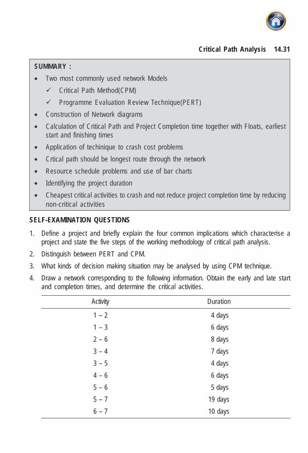
14.31Critical Path Analysis
SUMMARY :
• Two most commonly used network Models
� Critical Path Method(CPM)
� Programme Evaluation Review Technique(PERT)
• Construction of Network diagrams
• Calculation of Critical Path and Project Completion time together with Floats, earlieststart and finishing times
• Application of techinique to crash cost problems
• Crtical path should be longest route through the network
• Resource schedule problems and use of bar charts
• Identifying the project duration
• Cheapest critical activities to crash and not reduce project completion time by reducingnon-critical activities
SELF-EXAMINATION QUESTIONS
1. Define a project and briefly explain the four common implications which characterise aproject and state the five steps of the working methodology of critical path analysis.
2. Distinguish between PERT and CPM.
3. What kinds of decision making situation may be analysed by using CPM technique.
4. Draw a network corresponding to the following information. Obtain the early and late startand completion times, and determine the critical activities.
Activity Duration
1 – 2 4 days
1 – 3 6 days
2 – 6 8 days
3 – 4 7 days
3 – 5 4 days
4 – 6 6 days
5 – 6 5 days
5 – 7 19 days
6 – 7 10 days

14.32 Advanced Management Accounting
5. A work project consists of twelve activities labelled A through L. Upon being asked to specifythe order in which the jobs had to be done, the managers answered as follows :
A, B and C are the first activities of the project and can start simultaneously and immediately;A and B precede D while B precedes E, F and H. Activities F and C precede G while E andH precede I and J. C, D, F and J precede K which in turn, precedes L. Further I, G and L arethe terminal activities of the project.
The completion times of the various activities are listed here :
Activity Time (days)A 6B 4C 10D 1E 6F 3G 14H 1I 9J 2K 7L 5
(a) Draw a network diagram corresponding to this project.
(b) Obtain the lengths of all the paths and determine critical path.
ANSWER TO SELF-EXAMINATION QUESTIONS
5. The network diagram is shown in Figure below :
4
2
1
3 7 8
5 9
6
E
B
C
A
D
G
F
HI
L
K
J
Figure 29

14.33Critical Path Analysis
The various paths and their lengths are as follows :
Path Length
1-3-7-8-9 19
1-2-3-7-8-9 17
1-2-4-5-7-8-9 19
1-2-5-7-8-9 24* Critical
1-2-5-9 19
1-2-4-5-9 14
1-2-6-7-8-9 19
1-2-6-9 21
1-6-7-8-9 22
1-6-9 24* Critical

15Programme Evaluationand Review Technique
LEARNING OBJECTIVES :
After studying this chapter, you will be able to :
� Explain generic term network analysis and such related terms as Critical PathAnalysis. Critical Path Method (CPM) and Programme Evaluation and ReviewTechnique (PERT).
� Work out how network analysis helps managers to plan when to start various tasksto monitor actual progress and to know when control action is needed to preventdelay in completion of the project
� Draw diagram and chart representing inter-relationships between various elementsof the project and finally establishing critical path
� Identify dummy activities
� Identify earliest event times and latest even times for each event
� Identify total float, free float and independent float
� Crash times, costs and consumption of resources
� Help in decision making about project times and resource allocation
� Calculate the probability of completing the network in a given time when multipletime estimates of activity duration are available
15.1 INTRODUCTION
Hitherto our emphasis has been on CPM which is applicable where activity durations canbe estimated from experience, past historical records and work study techniques fairlyprecisely. CPM is incapable of handling uncertainty in timing which is a rule rather than aexpection for innovational projects such as introducing a new product or oil explorationproject. PERT (Program Evaluation and Review Technique) is more relevant for handingsuch projects which have a great deal of uncertainity associated with the activity durations.

15.2 Advanced Management Accounting
To take these uncertainity into account, three kinds of times estimates are generally obtained.These are:
(a) The Optimistic Times Estimate : This is the estimate of the shortest possible time inwhich an activity can be completed under ideal conditions. For this estimate, no provisionfor delays or setbacks are made. We shall denote this estimate by to.
(b) The Pessimistic Time Estimate : This is the maximum possible time which an activitycould take to accomplish the job. If everything went wrong and abnormal situations prevailed,this would be the time estimate. It is denoted by tp.
(c) The Most Likely Time Estimate : This is a time estimate of an activity which lies betweenthe optimistic and the pessimistic time estimates. It assumes that things go in a normal waywith few setbacks. It is represents by tm.
Beta distribution is a assumed for these “guess estimates” and PERT analysts have foundthat beta-distribution curve happens to give fairly satisfactory results for most of the activities.For a distribution of this type, the standard deviation is approximately one sixth of the range,i.e.
-
6
p o
t
t tS =
The variance, therefore; is
2 2 -
6
p o
t
t tS
⎛ ⎞= ⎜ ⎟⎝ ⎠
Exppected time : The expected time (te) is the average time taken for the completion ofthe job. By using beta-distribution, the expcetion time can be obtianed by following formula.
4
6
o m p
e
t t tt
+ +=
Probability estimate in PERT : Those experience and possessing expertise in the varioustechnical aspects of the projects are required to make three times estimates from which iscomputed t
e the expected times and S
t the standard deviation of the activity duration. The
expected time may then be used as the activity duration and the critical path may be foundby the analytical method explained earlier. But to what use is St put? Well this provides quitea useful information at the expense of completing a project by a given date. Here is theprocedure.
15.2 PROBABILITY OF ACHIEVING COMPLETION DATE
Suppose we wish to find out the probability that a project will be completed with thescheduled completion time. The time te as determined by b distribution after taking intoaccount three times estimates viz. to, tp and tm only represents a fifty pre cent chance thatthe activity will be completed with the time te. If the distribution curve for activity-i-j is as

15.3Programme Evaluation and Review Technique
shown in the following figure, the vertical line corresponding to te would divide the area
under the curve into two equal parts and the probability of completing the job in time tewould be ½. The probability of completing job within some other time Σ would be the areaunder curve upto the verticial line at Σ divided by the total area under the following curve,i.e. the probability of completing of completing the activity i-j within time Σ is P, then
area under ACEP=
area under ACB
Figure 1
In general, a project consisting of several activities will have a normal distribution, that is,or the project as a whole, the distribution cuvre is as shown below, and the probability ofcompleting the project in time is equal to the mean value Te which is ½.
Figure 2
If the scheduled time is Ts, the probability of completing the project within time Ts is theratio,
area under ACEP=
area under ACB
PR
OB
AB
ILIT
Y F
UN
CTI
ON

15.4 Advanced Management Accounting
In order to apply the above analysis to a network it is necessary to reduce the random curveobtained from the particular network into normal form. The advantage of this is that we canuse information and data available about the normal curve in the books of Statistics.
A standardized normal curve has an area equal to unity and a standard deviation ‘I’. further,it is symmetrical about the mean value te. Hence the area under the curve AC is 50% of thetotal area under the curve ACB. The area under the curve ACD depends on the location ofTs along the time axis. The point te can be taken as the reference point and the distance te.Ts can expressed in terms of standard deviation. For example, if Ts is on the right te at adistance of 1 standard deviation then the area enclosed by ACD is 84.1%. If Ts is on the leftof te at a distance of 1 standard deviation then area enclosed is 15.9%. These facts can bestated in a distance of -1 corresponds to 15.9% probability. By using proper statistical tablesand using the probabilities as obtained above, the value of standard normal variate (Z) canbe determined. But we know from statistics that
1 cpT –TZ =
. .S D
where T1 denotes the duration in which we wish to complete the project and T
cp represent
the duration on the critical path, S.D. stnds for standard deviation of the earliest finish ofa nwetwok.
Complute variance, Vt (=S2t) of all the activity duraitons of the critical path. Sum these up
and take square root. This yields the S.D. of the earliest finish time of a network. Let thecritical path duration be designeted by T
cp. Assuming normal distribution for the total duration,
you should be in a position to find the confidence interval for Tcp
. Note that 3SD give thelimits of the total possible duration with 99% confidence. Put it in another way.
Suppose you wish that the project be completed within a duration to T1. Find T1–Tcp
Z,SD
=
the standard normal variate.
Look to the standard normal probability distribution tables (Appendix 1) for the probability ofcompleting the projcet within the given duration of T1.
Illustration
If the critical path of a project is 20 months alongwith a standard duration of 4 months, whatis the probability that the project will be completed within :
(a) 20 months (b) 18 months (c) 24 months?
Solution
(a)20–20
Z = 4
= 0; Probability = 0.50
(b)18–20
Z = 4
= –0.50; Probability = 0.31
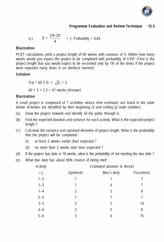
15.5Programme Evaluation and Review Technique
(c)24–20
Z = 4
= 1; Probability = 0.84
Illustration
PERT calculations yield a project length of 60 weeks with variance of 9. Within how manyweeks would you expect the project to be completed with probability of 0.99? (That is theproject length that you would expect to be exceeded only by 1% of the times if the projectwere repeated many times is an identical manner).
Solution
Tcp = 60 S.D. = 9 = 3.
60 + 3 × 2.3 = 67 weeks (Answer)
Illustration
A small project is composed of 7 activities whose time estimates are listed in the tablebelow. Activities are identified by their beginning (i) and ending (j) node numbers.
(a) Draw the project network and identify all the paths through it.
(b) Find the expected duration and variance for each activity. What is the expected projectlength ?
(c) Calculate the variance and standard deviation of project length. What is the probabilitythat the project will be completed :
(i) at least 3 weeks earlier than expected ?
(ii) no more than 3 weeks later than expected ?
(d) If the project due date is 18 weeks, what is the probability of not meeting the due date ?
(e) What due date has about 90% chance of being met?
Activity Estimated duration in Weeks
i–j Optimistic Most Likely Pessimistic
1–2 1 1 7
1–3 1 4 7
1–4 2 2 8
2–5 1 1 1
3–5 2 5 14
4–6 2 5 8
5–6 3 6 15

15.6 Advanced Management Accounting
Solution
(a) The nework is drawn in Fig. 3. The various paths are as follows.
Figure 3
(b) Expected duration and variances for various activities are compluted below.
te
Vt
1+1×4+7 7 –1
1–2; 2; = 16 6
⎡ ⎤= ⎢ ⎥⎣ ⎦
1+16+7 7 –1
1–3; 4; = 16 6
⎡ ⎤= ⎢ ⎥⎣ ⎦
2+8+8 8 – 2
1–4; 3; = 16 6
⎡ ⎤= ⎢ ⎥⎣ ⎦
1+4+1 1 –1
2–5; 1; = 06 6
⎡ ⎤= ⎢ ⎥⎣ ⎦
2+20+14 14 – 2
3–5; 1; = 46 6
⎡ ⎤= ⎢ ⎥⎣ ⎦
2+20+8 8 – 2
4–6; 1; = 16 6
⎡ ⎤= ⎢ ⎥⎣ ⎦
3+24+15 15 – 3
5–6; 7; = 46 6
⎡ ⎤= ⎢ ⎥⎣ ⎦
2

15.7Programme Evaluation and Review Technique
(c) Expected project Length = 17 weeks (Answer)
Variance of the critical path 1–3–5–6 = 1+4+4 = 9 (Answer)
∴Standard Deviation = 9 = 3 (Answer)
(i) Probability = 0.159 (Answer)
(ii) Probability = 0.841 (Answer)
(d) Tcp
= 17; T1 = 18;
Therefore, probability of meeting the due date = 0.63.
And probability of not meeting the date = 0.37 (=1–0.63)
(e) At 90% Probability, Z = 1.3 approximately.
∴1.3 = or T2 = 20.9 weeks approximately.
IllustrationFind event variances in the network of previous illustration.
SolutionEvent variance for both the TE and TL of each event are derived below. The computationalprocedure should be self evident. We shall put to use hte variances of the various activitiesderive in part (b) of solution to example 3 above.
Earliest Time, TE (D=Duration)Event Longest path leading to it *Variance
1 Nill (D=0) 0
2 1–2 (D=2) 1
3 1–3 (D=3) 1
4 1–4 (D=4) 1
5 1–3, 3–5 (D = 4 + 6 = 10) 1 + 4 = 5
6 1–3, 3–5, 5–6 (D=17) 1 + 4 + 4 = 9
Suppose we wish to find the projbability of reaching event 5 in 9 days. This can be computedas below:
* (N.B. If there are two equal longest path, higher of the two variances would be picked up).

15.8 Advanced Management Accounting
Probability (from Appendix 1) of reaching event 5 in 9 days is equal to 0.5 – .1723 = .3275.Likewise we can determine probabilities of reaching other events.
Longest Time TL
Event Longest path from it to last event 6 Variance
1 1–3, 3–5, 5–6 9
2 2–5, 5–6 4
3 3–5, 5–6 8
4 4–6 1
5 5–6 4
6 Nill 0
Illustration
Shown below is a PERT network and a related set of activity times:
i–j A B C D E F G H I J K L
to 10 12 8 4 0 12 6 9 4 0 5 9
tm 13 15 11 7 0 18 12 12 6 0 8 12
tp 22 18 20 16 0 36 18 27 8 0 11 33
Figure 4
Required
(a) Determine the expected completion time of each activtiy.
(b) Determine the earliest expected completion time, the latest expected completiontime and float of each activity.
2

15.9Programme Evaluation and Review Technique
(c) What is the total project completion time, and what are activities on the criticalpath?
(d) Determine S.D. of expected completion time for only those activities on the criticalpath.
(e) Determine the probability that the project will be completed within 41 weeks.
Solution
Figure 5
p m o p ot + 4t + t t – tte = ;
6 6⎛ ⎞= ⎜ ⎟⎝ ⎠
Time estimates Start Finishi–j t
o4t
mtp
te
E L E L Float Vt
S.D
1–2 10 52 22 14 0 17 14 31 171–3 8 44 20 12 0 0 12 12 0 4 21–4 12 60 18 15 0 10 15 25 102–6 4 28 16 8 14 31 22 39 173–4 0 0 0 0 12 25 12 25 133–5 12 72 36 20 12 12 32 32 0 16 43–7 6 48 18 12 12 20 24 32 84–6 9 48 27 14 15 25 29 39 105–6 4 24 8 6 32 33 38 39 15–7 0 0 0 0 32 32 32 32 0 0 06–8 5 32 11 8 38 39 46 47 1
7–8 9 48 33 15 32 32 47 47 0 16 4
tV = 36∑

15.10 Advanced Management Accounting
Hence S.D. of the critical path = 36 = 6.
Probability of completion critical path in 41 weeks is computed below:
41 – 47z = –1.
6=
∴ Probability = 0.159 (Answer).
Exercise
1. The following table lists the jobs of a network alongwith their time estimates.
i–j Optimistic Most Likely Pesstimistic
Duration Duration Duration
1–2 3 6 15
1–6 2 5 14
2–3 6 12 30
2–4 2 5 8
3–5 5 11 17
4–5 3 6 15
5–8 1 4 7
6–7 3 9 26
7–8 4 19 28
(a) Draw the project network.
(b) Calculate the length and variance of critical path.
(c) What is the approximate probability that jobs on the critical path will be completed bythe due date of 41 days?
(d) What is the approximate probability that jobs on the next most critical path will becompleted by the due date?
Answer : (b) Length = 36 days; Variance = 25; (c) 0.84; (d) 0.84
2. Below are given the three times estimates of each activity of a project network.Construct the network. Find the variance of each activity and variances of T
E and T
L of each
event.
i–j 1–2 1–3 1–4 2–5 3–5 4–6 5–6
to 7 15 7 9 20 14 2
tm
10 18 8 12 24 18 3
tp
12 20 9 17 26 20 7

15.11Programme Evaluation and Review Technique
Answer :
T E T L
i–j Variance Event No Variance Event No Variance1–2 0.69 1 0 1 2.141–3 0.45 2 0.69 2 2.461–4 0.11 3 0.45 3 1.692–5 1.77 4 0.11 4 1.003–5 1.00 5 1.45 5 0.694–6 1.00 6 2.14 6 05–6 0.69
15.3 A FEW COMMENTS ON ASSUMPTIONS OF PERT & CPM
1. Beta distribution may not always be applicable.
2. The formulae for the expected duration and S.D. are simplifications. Maccrinnon andRyavec reached the conclusion that in certain cases the errors, because of theseassumption, may even be to the tune of 33%.
3. The errors owing to the aforesaid simplification and assumption may be compoundedor may cancel each other to an extent.
4. In computing the S.D. of the critical path independence of activities is implied.Limitations of resources may invalidate the independence which exists by the verydefinition of an activity.
5. It may not always be possible to sort out completely identifiable activities and to statewhere they begin and where they end.
6. In projects fraught with in certainty it is natural that there exist alternatives with differingoutcomes. For example, if a particular hardness is not obtained in a metal, an alloymight have to be used that is more expensive and also inferior on certain technicalconsiderations. There have been theoretical developments in this regard, and it maybe worthwhile to incorporate the concept of decision tree analysis depending uponthe situation.
7. Time estimates have an element of subjectiveness and, to that extent, the techniquescould be weak. The contractors react to this weakness shrewdly whilst bidding. Ifthere are cost plus contracts they would deliberately “under estimate” the time forchances of being awarded with the contract. Incentive type contracts might lead toan opposite bias.
8. Cost-time trade offs, for deriving the cost curve slopes, to be discussed soon, aresubjective again and call for a great deal of expertise of the technology as well asgenuine effort to estimate. Often the engineers tend to be lax here; occasionally withthe honest deliberation event, the guesses may be wide off the mark.

15.12 Advanced Management Accounting
15.4 DISTINCTION BETWEEN PERT AND CPM
The PERT and CPM models are similar in terms of their basic structure, rationale andmode of analysis. However, there are certain distinctions between PERT and CPM networkswhich are enumerated below: .
(i) CPM is activity oriented i.e. CPM network is built on the basis of activities. Also resultsof various calculations are considered in terms of activities of the project. On theother hand, PERT is event oriented.
(ii) CPM is a determistic model i.e. It does not take into account the uncertainties involvedin the estimation of time for execution of a job or an activity. It completely ignores theprobabilistic element of the problem. PERT, however, is a probabilistic model. It usesthree estimates of the activity time; optimistic, pessimistic and most likely; with a viewto take into account time uncertainty. Thus, the expected duration of each activity isprobabilistic and expected duration indicates that there is fifty per cent probability ofgetting the job done within that time.
(iii) CPM places dual emphasis on time and cost and evaluates the trade-off betweenproject cost and project time. By deploying, additional resources, it allows the criticalpath project manager to manipulate project duration within certain limits so thatproject duration can be shortened at an optimal cost. On the other hand, PERT isprimarily concerned with time. It helps the manager to schedule and coordinatevarious activities so that the project can be completed on scheduled time.
(iv) CPM is commonly used for those projects which are repetitive in nature and whereone has prior experience of handling similar projects. PERT is generally used forthose projects where time required to complete various activities are not known aspriori. Thus, PERT is widely used for planning and scheduling research anddevelopment projects.
15.5 UPDATING THE NETWORK
The progress of various activities in a project network is measured periodically. Normally,either most of the activities are ahead or behind the schedule. It is therefore, necessary toupdate or redraw the network periodically to know the exact position of completion of eachactivity of the project. The task of updating the network may be carried out once in a month.Sometimes the updating of the network may provide useful information to such an extentthat it may demand the revision of even those very activities which have not started. Eventhe logic may also change i.e. some of the existing activities may have to be dropped andnew activities may be added up. In brief the network should be amended accordingly in thelight of new developments.
It is also not unlikely that the total physical quantum of work accomplished at a point of timemay exceed what was planned but the progress against the critical path alone may beslower than the scheduled pace. To understand how the task of updating is carried out,consider the following example:

15.13Programme Evaluation and Review Technique
Illustration
After 15 days of working the following progress is noted for the network of an erection job.
a) Activity 1-2, 1-3 and 1-4 completed as per original schedule.
b) Activity 2-4 is in progress and will be completed in 3 more days.
c) Activity 3-6 is in progress and will need 18 days more for completion.
d) Activity 6-7 appears to present some problem and its new estimated time of completionis 12 days.
e) Activity 6-8 can be completed in 5 days instead of originally planned for 7 days.
Figure 6
You are required to :
(i) Update the above diagram after 15 days of the start of work based on the assumptionsgiven above.
(ii) Write down the critical path with total project duration.
Solution
The new formulation of the problem is as follows:
(i) Activities 1-2, 1-3 and 1- 4 need 9, 10 and 6 days respectively as per originalprogramme.
(ii) Activity 2-4 needs 15 + 3-9 = 9 days instead of original programme of 7 days.
(iii) Activity 3-6 needs 15 + 18 -10 = 23 days.
(iv) Activity 3-4 needs 5 days.
(v) Activities 2-5, 4-7 and 5-7 need 18, 20 and 8 days respectively.
(vi) Activity 6-7 needs 12 days as no work was scheduled to be started for this activity on15th day.
(vii) Activities 6-8 and 7-8 need 5 and 6 days respectively.

15.14 Advanced Management Accounting
The new diagram based on the above listed activities will be as follows:
Figure 8
15.6 PROJECT CRASHING
In the discussion on PERT, we saw how the probability of completion of a project can becomputed for a specified duration. There are usually compelling reasons to complete theproject earlier than the originally estimated duration of the critical path computed on thebasis of normal activity times, by employing extra resources. An example would be introductionof a new project. The motive in hastening the project might be to ensure that the competitorsdo not steal a march. In the present section we will deal with those situations which willspeak of the effect of increase or decrease in the total duration for the completion of aproject and are closely associated with cost considerations. In such cases when the timeduration is reduced, the project cost increases, but in some exceptional cases project costis reduced as well. The reduction in cost occurs in the case of those projects which makeuse of a certain type of resources, for example, a machine and whose time is more valuablethan the operator’s time. Before we take up an example of project cost control, it is better tounderstand well the following preliminaries and their definitions.
Activity Cost : It is defined as the cost of performing and completing a particularactivity or task.
Crash Cost Cc : This is the direct cost that is anticipated in completing an activitywithin the crash time.
Crash time, Ct : This is the minimum time required to complete an activity.
Normal Cost, Nc : This is the lowest possible direct cost required to complete anactivity.
Normal time, Nt : This is the minimum time required to complete an activity at normalcost.
Activity cost slope: The cost slope indicates the additional cost incurred per unit of timesaved in reducing the duration of an activity. It can be understood more clearly by consideringthe figure 8.

15.15Programme Evaluation and Review Technique
Let OA represent the normal time duration for completing a job and OC the normal costinvolved to complete the job. Assume that the management wish to reduce the time ofcompleting the job to OB from normal time OA. Therefore under such a situation the cost ofthe project increases and it goes up to say OD (Crash Cost). This only amounts to savingthat by reducing the time period by BA the cost has increased by the amount CD. The rateof increase in the cost of activity per unit with a decrease in time is known as cost slope andis described as below.
Figure 8
CD OD – OCActivity cost slope =
AB OA – OB=
Crash Cost – Normal Cost
Tormal Time – Crash Time=
Optimum duration : The total project cost is the sum of the direct and the indirectcosts. In case the direct cost varies with the project duration time, the total project costwould have the shape indicated in the following figure:

15.16 Advanced Management Accounting
Figure 9
At the point A, the cost will be minimum. The time corresponding, to this point A is calledthe optimum duration and the cost as optimum cost for the project.The example below which the student should go through carefully is intended to explaincost implications of hastening a project.IllustrationThe following data pertains to the network drawn in figure 10-A given on the next page. It isdesired to compress the project to the least possible duration day by day and estimate theextra cost.
i–j Tn
Te
Cost slope1–2 3 2 7001–3 7 4 2002–3 5 3 1002–4 8 6 2003–4 4 2 400
SolutionThe critical path is 1-2-3-4 in figure A. It can be, seen that the critical path 1-2-3-4 is longer thaneither of the paths; 1-3-4 and 1-2-4 by one day. Therefore, the project can be compressed byone day along the critical path, 2-3 having the least cost slope is therefore crashed by a day.The revised network is depicted in figure B where all activities have become critical. Thefollowing choices of compression exist now. Each set of activities is so chosen that itreduces all the paths by a day.Crash each activity in one of the following sets by a day.
1–2 2–4 1–31–3 3–4 2–3
2–4Cost = 900 Cost = 600 Cost = 500
The last set of crashing 1-3, 2-3 and 2-4 is the least expensive and these activities arecrashed accordingly.

15.17Programme Evaluation and Review Technique
Figure 10 [(A) to (E)]

15.18 Advanced Management Accounting
Extra cost = 200
100
200
Rs. 500
This is shown in figure C. Activity 2-3 having been crashed to the limit is dropped out fromfurther consideration. In C. the following choices of crashing each activity a day exist:
1–2 1–3 2–4
3–4 1–2 3–4
Extra cost Rs. 1100 Rs. 900 Rs. 600
Extra cost The last is selected Extra Cost = Rs. 600
The revised network is shown in figure D where 2-4 joins 2-3 in that it is also crashed tolimit. The only possibility of compressing the network in figure D is to crash 1-2 and 1-3 bya day each. This is done and the final network is shown in figure E.
Extra cost = Rs. 900
Although 1-3 and 34 have not reached their crashing limits in figure E there is no use alsoto crash these since this would not compress the project which can be compressed to 8days only.
Total extra cost = 100 + 500 + 600 + 900 = Rs. 2.100.
[If. however. just the least duration plan was required one could go about the problem in amuch simpler way as follows. Draw the network with te’s. This is done in the figure 10F.
Figure 10 (F)
The network is analysed with 1-24 as the critical path of 8 day’s duration. The other pathshave to be contracted to 8 day’s duration. This can be done in one of the following ways:(i) Increase 1-3 and 3-4 by a day each with cost reduction of Rs. 200 + 400 = 600.(ii) Increase 2-3 and 1-3 by a day and 2 days respectively with cost reduction of Rs. 100
+ 400 = 500.

15.19Programme Evaluation and Review Technique
Obviously the 1st course is to be preferred and the network. if now revised. would beidentical with the one of figure E.
Often. however. management would be interested in the least total cost duration rather thanthe least possible duration.Now, suppose there is an indirect cost of Rs. 800 per day. What would then be the least costproject duration for the example on hand ? The various cost data are tabulated below:
Duration Direct (Crashing) cost Indirect cost Total cost12 0 9600 960011 100 8800 890010 600 8000 8600
9 1200 7200 84008 2100 6400 8500
Thus 9 days is the least toal cost duration and rationally the management should go in forthis unless high opportunity losses compel them to select a lower duration project plan.IllustrationConsider the following network and the table for a particular project which consists of 7activities.
Figure 11
(The number indicated along the activity arrows are the normal duration.)
Activity Noraml Crash Cost slopesTimes Cost Time Cost ΔT ΔC ΔC/ΔT(days) Rs. (days) Rs.
1–2 3 360 2 400 1 40 40 2–3 6 1440 4 1620 2 180 90 2–4 9 2160 5 2380 4 220 55 2–5 7 1120 5 1600 2 480 240 3–4 8 400 4 80 4 400 100 4–5 5 1600 3 1770 2 170 85 5–6 3 480 2 760 1 280 280
7560 9330The indirect cost is Rs. 160/-per day. Determine optimum duration in the above case.

15.20 Advanced Management Accounting
Solution
The normal duration of the project is obtained from the critical path and not by merelysumming up the normal duration of all the activities. The overall normal duration in theabove project is 25 days and the total direct cost is Rs. 7560/-. If due to some reason it isfelt that the project is to be hastened, the question then to be answered is: “what is theminimum time required for the completion of the project?”
According to the crash time given in the table; the critical path based on these crash timeestimates still appears as 1-2-3-4-5-6 and the crash duration is 15 days. Hence, the projectmay take 15 to 25 days depending upon the money the management is prepared to spend.If the management decides to complete the project in 15 days, then the direct cost will beRs. 9330/-. The figure has been arrived by speeding up or crashing all the activities asmentioned in the, given table. But there are several non-critical activities in the project,which need not be crashed to reduce the project duration. Speeding up of such non criticalactivities involves extra amount. As any extra amount spent on these activities is not going toreduce the project duration, therefore it is better not to reduce the duration of these non-critical activities. Duration of these non-critical activities should be reduced only when theybecome critical activities, during the process of reducing the project duration time.
The two objectives behind the reduction of project time are:
(1) To complete the project before a certain target date.
(2) To reduce the overall cost of the project. This objective can only be achieved whenthe indirect cost per day is greater than some of the cost slopes as given in the table.In the exercise under consideration, the five activities 1-2, 2-3, 2-4, 3-4 and 4-5 havecost slopes lower than the indirect cost. In such a situation, the management wouldbe very much interested in cutting down the project time, thereby decreasing the totalindirect cost. In order to solve this example we proceed as follows:
First step is to identify those activities along the critical path whose cost slopes are lessthan the indirect cost. In our network such activities are 1-2,2-3,3-4 and 4-5. We take theseactivities in the order of increasing cost slopes. Activity 1-2 has a slope of Rs. 40/per day.This activity can be cut down by 1 day at a cost of Rs. 40/-. The next activity in the order ofcheapness is 4-5. This can be cut down by 2 days at a cost of E-s. 170. Next we may takethe activity 2-3 whose cost slope is Rs. 90/-. This activity can be contracted by 2 days at acost of Rs. 180. So far three activities viz. 1-2,4-5 and 2-3 have been contracted by a totalof 5 days at an overall cost of Rs, 390/-.
From the given table, we notice that the next activity in the order of priority is 3-4 with a costslope Rs. 100/- per day. This activity can be cut down by 4 days. But a look on the networkafter the performance of above reduction in time reveals that activity 2-4 has float of only 3days.

15.21Programme Evaluation and Review Technique
Figure 12
Hence we can not cut down the duration for the activity 3-4 by four days without affecting theactivity 2-4. Therefore one should cut down the duration on activity 3-4 by 3 days at a costof Rs. 300/- and now by this process a new sub-critical path viz. 1-2-4-5-6 may come intoexistence.
According to the given Table, activity 3-4 can be further contracted by 1 day. But this cannotbe achieved without contracting activity 2-4. Therefore, the cost slope must include both ofthese activities i.e. activities 2-4 and 3-4. The combined cost slope of these : two activitiesis Rs. 55 + Rs. 100 = Rs. 155. The project duration has now been reduced to 116 days, asbelow:
Activity Duation reduced by Cost slope Cost of contraction
(Days) (Rs.) (Rs.)
1–2 1 40/- 40/-
4–5 2 85/- 170/-
2–3 2 90/- 180/-
3–4 3 100/- 300/-
3–4,2–4 1 155/- 155/-
9 845/-
During the above process a total reduction of 9 days has been achieved at an extra cost ofRs. 845/-. Also the indirect cost @ Rs. 160/- per day for 9 days resulting in Rs. 1440/- hasbeen saved.
In other words, the project duration has been reduced from 25 days to 16 days. As a resultof this duration of project its direct cost has now become Rs. 8405/- and Rs. 2560/- as itsindirect cost. The overall project cost with the new time schedule i.e. 16 days is Rs. 8405 +Rs. 2560 = Rs. 10965/- as against the overall cost of Rs. 11560, it thus results in a netsaving of Rs. 595/-
Exercise 3. A small maintenance project consists of jobs in the table below. With each jobis listed its normal time and a minimum, or crash time, in days. The cost (in Rs. per day) ofeach job is also given.

15.22 Advanced Management Accounting
Job Normal day Minimum (crash) Cost/day
i-j duration day duration
1-2 9 6 20
1-3 8 5 25
1-4 15 10 30
2-4 5 3 10
3-4 10 6 15
4-5 2 1 40
(a) What is the normal project length and the minimum project length?
(b) Determine the minimum crashing cost of schedules ranging from normal length downto, and including, the minimum length schedule. That is, if L = length of the schedule,find the costs of schedules which are L, L - 1, L-2 and so on days long.
(c) Overhead costs total Rs. 60 per day. What is the optimum length schedule in terms ofboth crashing and overhead cost? List the scheduled duration of each job for your solution:
Answer : (a) 20 days: 12 days
(b) Length (days Crashing Cost Total Cost
Rs. Rs.
20 0 1200
19 15 1155
18 30 1110
17 45 1065
16 85 1045
15 130 1030
14 195 1035
13 260 1040
12 335 1055
(c) Optimum length = 15 days.
Illustration
The Arcot Machinery Company has been offered a contract to build and deliver nineextruding pressess to the Home Bottling Company. The contract price negotiated iscontingent upon meeting a specified delivery time, with a bonus offerd for early delivery.The marketing department has established the following cost and time information:

15.23Programme Evaluation and Review Technique
Normal time (weeks) Normal Cost Crash Time Crash Cost
Activity a b m (Rs.) (weeks) (Rs.)
1–2 1 5 3 5000 1 9000
2–3 1 7 4 8000 3 14000
2–4 1 5 3 4000 2 6000
2–5 5 11 8 5000 7 6000
3–6 2 6 4 3000 2 5000
4–6 5 7 6 2000 4 3600
5–7 4 6 5 10000 4 14000
6–7 1 5 3 7000 1 10600
Normal delivery time is 16 weeks for a contract price of Rs. 62,000.
On the basis of the calculated profitability for each delivery time specified in the followingtable, what delivery schedule do you recommend that the company may implement?
Contract Delivery Time Contract Amount
(weeks) (Rs.)
15 62,500
14 65,000
13 70,000
12 72,500
(Here a = to : optimistic time, b=tp; pessimistic time, m=tm; most likely time.)
Solution
Let us first calculate the expect duration of each activity.
Normal Time (weeks) Expected Normal Crash Crash Cost
Activity a b m duration Cost T ime Cost Slope
(weeks) Rs. (weeks) (Rs.)
1-2 1 5 3 3 5000 1 9000 2000
2-3 1 7 4 4 8000 3 14000 6000
2-4 1 5 3 3 4000 2 6000 2000
2-5 5 11 8 8 5000 7 6000 1000
3-6 2 6 4 4 3000 2 5000 1000
4-6 5 7 6 6 2000 4 3600 800
5-7 4 6 5 5 10000 4 14000 4000
6-7 1 5 3 3 7000 1 10600 1800

15.24 Advanced Management Accounting
The network for the given problem is drawn below:
Figure 13
The critical path is 1-2-5-7 with total duration 0116 weeks. Cost of all activities is Rs.44,000.Contract price is Rs. 62,000 for normal delivery time of 16 weeks. Hence the profit is of Rs.18000.
For calculating the most profitable delivery schedule, let us start crashing the activities onthe critical path. Cost slopes for various activities are given in the above table.
Step 1: The critical activity 2-5 has the least cost slope of Rs. 1,000, so we crash thisactivity by 1 day. Crashing cost is Rs. 1000. The contract amount for delivery time of 15weeks is Rs. 62,500
Profit = Rs. 62,500 - (Rs. 44,000 + Rs. 1,000)
= Rs. 62,500 -Rs. 45,000 = Rs. 17,500
Step 2: Now there are two critical paths viz. 1-2-4-6-7 and 1-2-5-7 with duration of 15 weeks. Sowe crash activity 1-2 by 1 day at crash cost of Rs. 2000. Project duration is 14 weeks.
Profit = Rs. 65,000 - Rs. (45,000 + 2,000) = Rs. 18,000.
Step 3: We again crash activity 1-2 by 1 day. So the project duration is 13 weeks
Profit = Rs. 70,000 - (Rs. 47,000 + Rs. 2,000)
= Rs. 70,000 - Rs. 49,000 = Rs. 21,000
Step 4: Now we crash activity 4-6 for path 1-2-4-6-7 at crash cost of Rs. 800 andactivity 5-7 for path 1-2-5-7 at crash cost of Rs. 4000. Project duration is now 12weeks.
Profit = Rs. 72,500 - (Rs. 49,000 + Rs. 4000 + Rs. 800)
= Rs. 72,500 - Rs. 53,800 = Rs. 18,700
No further crashing is possible.
From step 3, it can be seen that the profit is maximum when the project duration is 13weeks. Hence, the company should implement the delivery schedule of 13 weeks at acontract amount of Rs. 70,000 to gain maximum profit of Rs. 21,000
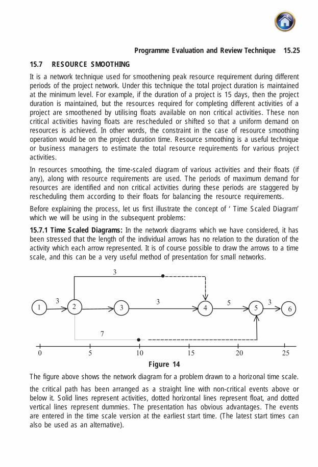
15.25Programme Evaluation and Review Technique
15.7 RESOURCE SMOOTHING
It is a network technique used for smoothening peak resource requirement during differentperiods of the project network. Under this technique the total project duration is maintainedat the minimum level. For example, if the duration of a project is 15 days, then the projectduration is maintained, but the resources required for completing different activities of aproject are smoothened by utilising floats available on non critical activities. These noncritical activities having floats are rescheduled or shifted so that a uniform demand onresources is achieved. In other words, the constraint in the case of resource smoothingoperation would be on the project duration time. Resource smoothing is a useful techniqueor business managers to estimate the total resource requirements for various projectactivities.
In resources smoothing, the time-scaled diagram of various activities and their floats (ifany), along with resource requirements are used. The periods of maximum demand forresources are identified and non critical activities during these periods are staggered byrescheduling them according to their floats for balancing the resource requirements.
Before explaining the process, let us first illustrate the concept of ‘ Time Scaled Diagram’which we will be using in the subsequent problems:
15.7.1 Time Scaled Diagrams: In the network diagrams which we have considered, it hasbeen stressed that the length of the individual arrows has no relation to the duration of theactivity which each arrow represented. It is of course possible to draw the arrows to a timescale, and this can be a very useful method of presentation for small networks.
Figure 14
The figure above shows the network diagram for a problem drawn to a horizonal time scale.
the critical path has been arranged as a straight line with non-critical events above orbelow it. Solid lines represent activities, dotted horizontal lines represent float, and dottedvertical lines represent dummies. The presentation has obvious advantages. The eventsare entered in the time scale version at the earliest start time. (The latest start times canalso be used as an alternative).

15.26 Advanced Management Accounting
Illustration
Consider a project consisting of thirteen activities having duration and resource requirementsshown below:
Activity Duration (days) Labourers required
A 2 2L
B 4 2C,2L
C 4 4C
D 3 2L
E 4 6C
F 7 2L
G 2 4C
H 5 4C,2L
J 2 2C
K 5 2C
L 2 2L
M 3 4L
N 2 4L
Here L stands for labourers and C stands for carpenters, we shall analyse this project fromthe point of view of resources to bring out the necessary steps involved in the analysis andsmoothing of resources.
From the values given in Table above Ei’s and Li’s are calculated and given in the networkbelow (fig. I 5)
The critical path for this network is 0–1–3–5–7–8–9–10 and is shown by dotted lines, Infigure 16 is shown the time-scaled version of the same network. The critical path is shownalong the horizontal line. The last two rows (also referred to as resource accumulationtable) in figure 16 give the number of abourers and carpenters required each day. It can beseen that the demand on the resources is not even. On the 7th and 8th days the demand forcarpenters is as high as 14, whereas on the 11th, 12th and 13th days it is two only. If thecarpenters and labourers are to be hired for the entire project duration of 22 days, thenduring most of the days they will be idle and the company will have to hire at leas L 14carpenters and 4 labourers.
We will attempt to re-schedule our activities in-such a way as to utilize the resources in a fairlyuniform manner. As mentioned above the maximum demand on the resources occurs on the6th, 7th, 8th, 9th and 10th days. The activities on these days will have to be shifted depending

15.27Programme Evaluation and Review Technique
Figure 15
upon their floats such that the demand comes down. As can be seen from the above time-scaled version, activity 3-8 has maximum float, therefore we will try to shift activity 3-8 sothat is starts on the 16th day instead of the 7th day. This reduces the demand on thecarpenters from 14 to 10 on the 7th and 8th days so that the maximum demand for thecarpenters on any day is now 10 and not 14. The modified resource accumulation tableand the time-scaled version of the project is shown on next page in figure 17.
Figure 16
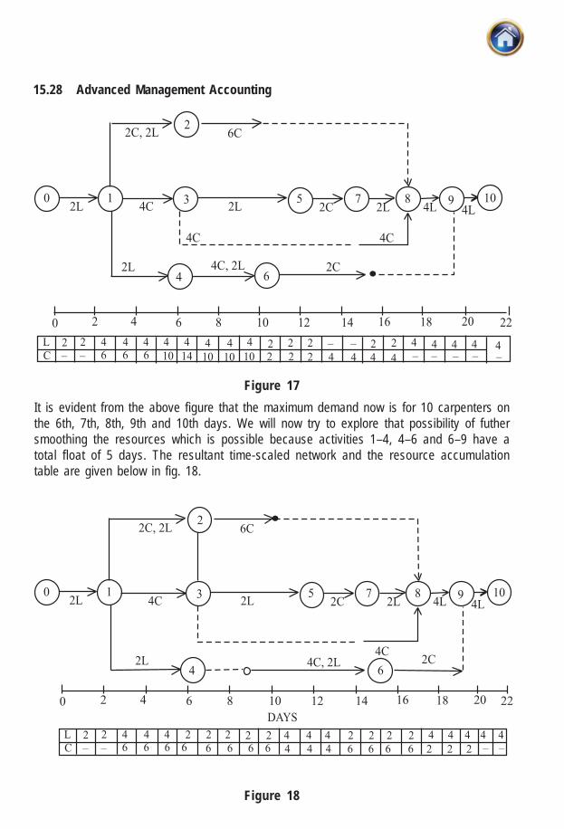
15.28 Advanced Management Accounting
Figure 17
It is evident from the above figure that the maximum demand now is for 10 carpenters onthe 6th, 7th, 8th, 9th and 10th days. We will now try to explore that possibility of futhersmoothing the resources which is possible because activities 1–4, 4–6 and 6–9 have atotal float of 5 days. The resultant time-scaled network and the resource accumulationtable are given below in fig. 18.
Figure 18

15.29Programme Evaluation and Review Technique
As can be seen from the above figure the requirement for labourers is 4 and the requirementfor carpenters reduces to 6 as against 14 carpenters originally estimated. Hence, byjudiciously utilizing the float, we can smooth the demand on the resources.
15.8 RESOURCE LEVELLING
It is also a network technique which is used for reducing the requirement of a particularresource due to its paucity. The process of resource levelling utilize the large floats availableon non-critical activities of the project and thus cuts down the demand on the resource. Inresource levelling, the maximum demand of a resource should not exceed the availablelimit at any point of time. In order to achieve this, non critical activities are rescheduled byutilising their floats. Some times, the use of resource levelling may lead to enlonging thecompletion time of the project. In other words, in resource levelling, constraint is on the limitof the resource availability.
15.9 MISCELLANEOUS ILLUSTRATIONS
Illustration
A project consists of eight activities with the following relevant information:
Activity Immediate Predecessor Estimated Duration (Days)
Optimistic Most Likely Pessimistic
A – 1 1 7
B – 1 4 7
C – 2 2 8
D A 1 1 1
E B 2 5 14
F C 2 5 8
G D,E 3 6 15
H F,G 1 2 3
(i) Draw the PERT network and find out the expected project completion time.
(ii) What duration will have 95% confidence for project completion?
(iii) If the average duration for activity F increases to 14 days, what will be its effect on theexpected project completion time which will have 95% confidence?

15.30 Advanced Management Accounting
Solution
(i) The required network is drawn below:
The expected time for each activity shown in the network above is calculated in the followingtable:
Activity Estimated Duration (Days) Expected Variance
Duration
a + 4m +b
b⎛ ⎞⎜ ⎟⎝ ⎠
b – a
b⎛ ⎞⎜ ⎟⎝ ⎠
A 1–2 1 1 7 2 1B 1–3 1 4 7 4 1C 1–4 2 2 8 3 1D 2–5 1 1 1 1 0E 3–5 2 5 14 6 4F 4–6 2 5 8 5 1G 5–6 3 6 15 7 4
H 6–7 1 2 3 2 1/9
The critical path is given by 1-3-5-6-7 or B-E-G-H and the expected project completion timeis 19 days. .
(ii) The variance for critical path is 1 + 4 + 4 + 1/9 = 82/9
Standard deviation of critical path = σ1 =82
9 = 3.02 (approx.)
To calculate the project duration which will have 95% chances of its completion, weutilise the value of Z corresponding to 95% confidence which is 1.645.
Optimistic Most likely Pessimistica m b

15.31Programme Evaluation and Review Technique
Thus, X – 19
3.02 = 1.645,
or X = 1.645 × 3.02 + 19 = 23.97 days = 24 days
Hence, 24 days of project completion time will have 95% probability of its completion.
(iii) If the average duration for activity F increases to 14 days, then the path 1-4-6-7 i.e.,C-F-H will also become critical path with expected project completion time of 19days. Now, activities C and F are also critical activities. Since we and, given only theaverage duration for activity F, it is assumed that the variance for this activity is zero.Further, since PERT analysis is based on the assumption that the activities areindependent in terms of their variance, therefore, standard deviation of critical pathscan be computed as:
1 = 1+4+4+ 0 1
9σ + + =
110 +
9 =318. approx
We now wish to calculate the expected project completion time that will have 95%confidence level,
P (Z < 1.645) = 0.95
X – X – 191.645
3.18
μσ
= =
or X = 19 + 1.645 x 3.18 = 24.23 days.
Hence the project duration of 24.23 days will have 95% confidence of completion.
Illustration
The following information is given below:
Activity (1–2) (2–3) (2–4) (3–5) (4–6) (5–6) (5–7) (6–7)
Pessimistic time 3 9 6 8 8 0 5 8
(in weeks)
Most likely time 3 6 4 6 6 0 4 5
(in weeks)
Optmistic time 3 3 2 4 4 0 3 2
(in weeks)
Draw the network diagram for the above. Calculate :
(i) Variance to each activity.
(ii) Critical path and expected project length.
(iii) The probability that the project will be completed in 23 weeks is drawn below:

15.32 Advanced Management Accounting
Solution
The required network is drawn below:
Figure 20
The expected time marked in the above network diagram for various activities is calculatedin the table below:
Times (in weeks) Expected VarianceActivities Optimistic Most like Pessimistic time (weeks)
(to) (t
m) (t
p)
0 m p
e
t +4t +tt =
6
p 0t – t
6⎛ ⎞⎜ ⎟⎝ ⎠
1–2 3 3 3 3 02–3 3 6 9 6 12–5 2 4 6 4 4/93–5 4 6 8 6 4/94–6 4 6 8 6 4/95–6 0 0 0 0 05–7 3 4 5 4 1/96–7 2 5 8 5 1
(i) Variance of each activities has been calculated in the last column of the above table.(ii) Critical path is given by 1–2–3–5–6–7 and the expected project length is 20 weeks.(iii) Variance of the critical path = σ2 = 0 + 4/9 + 0 + 1 = 22/9 = 2.444
Mean = x = 20 weeksTo calculate the probability of completing the project in 23 weeks, we will first calculate thenormal Z as below:
D – x 23 20Z = 1.92
2.444σ−= =
P (x < 23) = P (z < 1.92) = 0.9726 (from the Normal table)Thus, the probability that the project will be completed in 23 weeks is 97.26%.

15.33Programme Evaluation and Review Technique
Illustration
A small maintenance project consists of the following twelve jobs whose precedencerelations are identified with their node number:
Job (i–j) (1,2) (1,3) (1,4) (2,3) (2,5) (2,6)
Duration (in days) 10 4 6 5 12 9
Job (i–j) (3,7) (4,5) (5,6) (6,7) (6,8) (7,8)
Duration (in days) 12 15 6 5 4 7
(i) Draw an arrow diagram representing the project.
Figure 21
(ii) Calculate earliest start, earliest finish, start and latest finish time for all jobs.
(iii) Find the critical path and project duration.
(iv) Tabulate total float, free float and independent float.
Solution : (i) The required arrow diagram is drawn in figure 21.

15.34 Advanced Management Accounting
(ii) The earliest start, earliest finish, latest start and latest finish time for all the jobs arecalculated in the table given below:
Job Dura- Ealiest time Latest time Slcak of Total Free Indep.
(ij) tion Start Finish Start Finish tail head float=TF float=FF floatin days EST EFT LST event event =(LST- =(TF- Stock)(FF-Slock)
(Ei) (Lj) (Li–Ej) (Lj–Ei) EAST) of head of tailevent event
1–2 10 0 10 0 10 0 0 0 0 01–3 4 0 4 17 21 0 6 17 11 111–4 6 0 6 1 7 0 1 1 0 02–3 5 10 15 16 21 0 6 6 0 02–5 12 10 22 10 22 0 0 0 0 02–6 9 10 19 19 28 0 0 9 9 93–7 12 15 27 21 33 6 0 6 6 04–5 15 6 21 7 22 1 0 1 1 05–6 6 22 28 22 28 0 0 0 0 06–7 5 28 33 28 33 0 0 0 0 06–8 4 28 32 36 40 0 0 8 8 87–8 7 33 40 33 40 0 0 0 0 0
(iii) The critical path is 1 2 5 6 7 8 and the project duration is 40 days.
(iv) Total float, free float and independent float for various activities are calculated in theabove table.
Illustration
A small project consists of seven activities for which the relevant data are given below:
Activity Preceding Activities Activities Duration
(Days)
A – 4
B – 7
C – 6
D A,B 5
E A,B 7
F C,D,E 6
G C,D,E 5
(i) Draw the network and find the project completion time.
(ii) Calculate total for each of the activities.
(iii) Draw the time scaled diagram.

15.35Programme Evaluation and Review Technique
Figure 22
Solution
(i) The required network is given in figure 22.
The critical path is 1–3–5–7 with duration of 20 days. Thus, the project completion times is20 days.
(ii) The total float for various activities is calculated as below:
Start Finish Total float
Activity Duration Earliest Latest Earliest Latest
A 1–2 4 0 3 4 7 3
B 1–3 7 0 0 7 7 0
C 1–4 6 0 8 6 14 8
Dummy 1 2–3 0 4 7 4 7 3
D 3–4 5 7 9 12 14 2
E 3–5 7 7 7 14 14 0
Dummy 2 4–5 0 12 17 12 14 2
F 5–7 6 14 17 20 20 0
G 5–6 5 14 15 19 20 1
Dummy 3 6–7 0 19 20 19 20 1
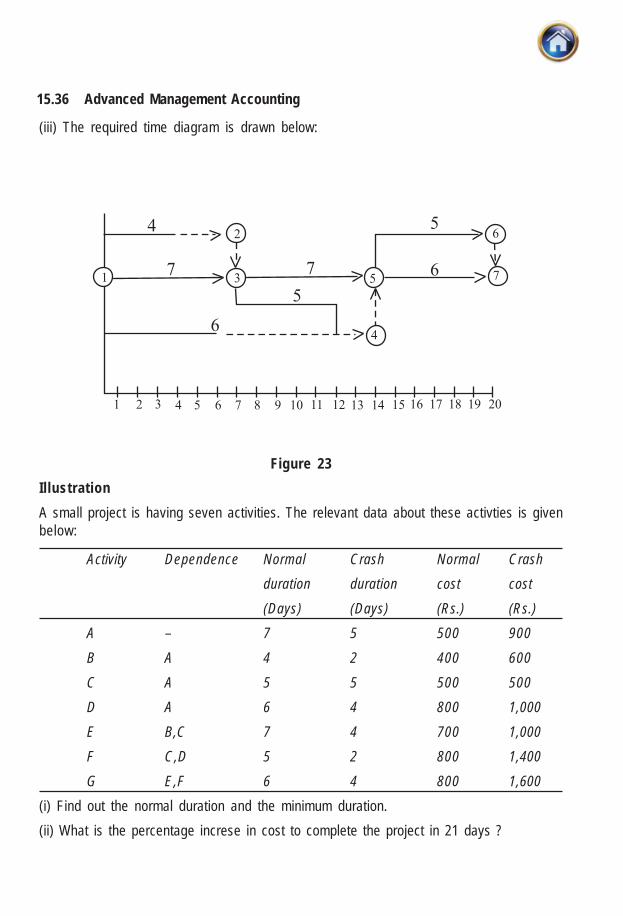
15.36 Advanced Management Accounting
(iii) The required time diagram is drawn below:
Figure 23
Illustration
A small project is having seven activities. The relevant data about these activties is givenbelow:
Activity Dependence Normal Crash Normal Crash
duration duration cost cost
(Days) (Days) (Rs.) (Rs.)
A – 7 5 500 900
B A 4 2 400 600
C A 5 5 500 500
D A 6 4 800 1,000
E B,C 7 4 700 1,000
F C,D 5 2 800 1,400
G E,F 6 4 800 1,600
(i) Find out the normal duration and the minimum duration.
(ii) What is the percentage increse in cost to complete the project in 21 days ?

15.37Programme Evaluation and Review Technique
Solution
The network is given below:
Figure 24
(i) The critical path of the project is A C E G or 1–2–3–4–6–7 with normal duration of25 days.
The minimum duration of the project is 18 days.
(ii) The cost slope for various activities is given below:
Activity Normal Crash Normal Crash Costduration duration cost(Rs.) cost(Rs.) slope (Rs.)
A(1-2) 7 5 500 900900 – 500
2007 – 5
=
B(2-4) 4 2 400 600600 – 400
1004 – 2
=
C(2-3) 5 5 500 500 N.A
D(2-5) 6 4 800 10001000 – 800
1006 – 4
=
E(4-6) 7 4 700 10001000 – 700
1007 – 4
=
F(5-6) 5 2 800 14001400 – 800
2005– 2
=
G(6-7) 6 4 800 16001600 – 800
4006 – 4
=
Total 4,500

15.38 Advanced Management Accounting
Step-I: Various paths of the network are given below:
1-2-3-4-6-7 with duration = 25 days
1-2-4-6-7 with duration = 24 days
1-2-3-5-6-7 with duration = 23 days
1-2-5-6-7 with duration = 24 days
In order to determine the cost of completing the project in 21 days, let us crash that activityon the critical path which has minimum cost slope. It can be seen that the minimum costslope of Rs. 100 corresponds to activity E( 4-6) and it lies on the critical path. Hence, wecrash activity E (4-6) by 1 day at an additional cost of Rs. 100.
Step-2: Various paths now are
1-2-3-4-6-7 with duration = 24 days
1-2-4-6-7 with duration = 23 days
1-2-3-5-6- 7 with duration = 23 days
1-2-5-’6-7 with duration = 24 days
An examination of the above four paths clearly points out that there are two critical pathsnamely 1-2-3-4-6-7 and 1-2-5-6-7, each with duration = 24 days. To reduce the projectduration by three days more, there are following possible combination of activities.
1. Crash activities 4 - 6 on the path 1-2-3-4-6-7 and 5 - 6 on the path 1-2-5-6-7 by one dayeach at an addition cost of Rs. 100 + Rs. 200 = Rs. 300
2. Crash activities 4-6 on path 1-2-3-4-6-7 and 2-5 on path 1-2-5-6-7 by one day each atan additional cost of Rs. 100 + Rs. 100 =Rs. 200
3. Crash activity 1-2 by one day at an additional cost of Rs. 200.
It can be observed that the additional cost of reducing the project duration by one day incombination 2 as well as combination 3 is Rs. 200. Hence any of these two can be selectedfor crashing. However, since crashing activity 1-2 by 1 day reduces the duration of all thepaths by 1 day, we will crash it by 1 day. The project duration becomes = 23 days at anadditional cost = Rs. 200.
Step-3: Crash activity 1-2 by 1 day further, it would reduce the project duration to 22 daysat an additional cost = Rs. 200.
Step-4: Activity 1-2 can not be crashed further. So, we now select the combination 2stated above for crashing. Crash activities 4-6 and 2-5 by one day each at anadditional cost of Rs. 100 + Rs. 100 = Rs. 200.
The project duration now becomes equal to 21 days.
Hence, in order to complete the project in 21 days, an additional cost of Rs. 100 + Rs. 200+Rs. 200 + Rs. 200 = Rs. 700 will be incurred.
The normal cost of completing the project in 25 days = Rs. 4500.

15.39Programme Evaluation and Review Technique
Hence, the percentage increase in cost to complete the project in
21 days = Rs. 700
100 15.5%Rs. 4500
× =
SUMMARY :Three kinds of times estimates� The Optimistic Time Estimate
� The Pessimistic Time Estimate
� The Most Likely Time Estimate
Variance : 2 2 -
6
p o
tt t
S⎛ ⎞= ⎜ ⎟⎝ ⎠
Expected time : The expected time (te) is the average time taken for the completion ofthe job. By using beta-distribution, the expcetion time can be obtianed by following formula.
4
6
o m p
e
t t tt
+ +=
Activity Cost : It is defined as the cost of performing and completing a particularactivity or task.
Crash Cost Cc :This is the direct cost that is anticipated in completing an activitywithin the crash time.
Crash time, Ct : This is the minimum time required to complete an activity.
Normal Cost, Nc : This is the lowest possible direct cost required to complete anactivity.
Normal time, Nt : This is the minimum time required to complete an activity at normalcost.
Activity cost slope : The cost slope indicates the additional cost incurred per unit oftime saved in reducing the duration of an activity
Resource smoothing
It is a network technique used for smoothening peak resource requirement during differentperiods of the project network. Under this technique the total project duration is maintainedat the minimum level.
Resource levellingIt is also a network technique which is used for reducing the requirement of a particularresource due to its paucity. The process of resource levelling utilize the large floatsavailable on non-critical activities of the project and thus cuts down the demand on theresource. In resource levelling, the maximum demand of a resource should notexceed the available limit at any point of time. In order to achieve this, non criticalactivities are rescheduled by utilising their floats.

15.40 Advanced Management Accounting
SELF-EXAMINATION QUESTIONS
1. Below we give a PERT network with the related time data. Your are required to findthe probability of completing the project in 27 days.
Figure 25
Activity A B C D E F G
ta 6 5 4 4 4 4 2
tm 9 8 7 7 7 10 5
tp 18 17 22 16 10 22 8
Answer : Critical path = 23 days, prob = 0.903.
2. The following table gives the activities in a construction project and other relevantinformation:
Activity Normal time Crash time Normal cost Total CrashDays days (Rs.) cost (Rs.)
1-2 20 17 600 7201-3 25 25 200 2002-3 10 8 300 4402-4 12 6 400 7003-4 5 2 300 4204-5 10 5 300 600
(a) Draw the network for the project.
(b) Find the total, free and independent floats for each activity.
(c) Using all information “crash” or “shorten” the project step by step until the shortestduration is reached. .

15.41Programme Evaluation and Review Technique
3. Projects India Limited undertakes special contracts. The following table givesestimates of time and cost for activities involved in completing one contract whichhas been just offered to them.
Activity Previous Normal time Normal cost Minimum Cost of
activities days (Rs.) time minimum time
A – 12 10,000 8 14,000
B – 10 5,000 10 5,000
C A 0 0 0 0
D A 6 4,000 4 5,000
E B,C 16 9,000 14 12,000
F D 16 3,200 8 8,000
60 31,200 44 44,000
“Previous activities” must be completed before the activity in question can be started. Theminimum time represents the shortest time in which the activity can be completed giventhe use of special costly methods of operation. Assume that it is possible to reduce thenormal time to the minimum time is small steps and the extra cost incurred will beproportional to the time saved.
(a) Draw a network diagram and identify the critical path for normal procedures
(b) Recommend what programme be followed if the job must be completed in 30 daysand calculate the total cost for the programme.
4. Alpha construction company has an opportunity to submit a bid for the constructionof a new apartment building. From specifications provided by the developer, a PERTnetwork for the project has been developed, and is shown below. Also shown for eachactivity are estimates of most optimistic, most likely, and most pessimistic completiontimes in weeks (a, m and b, respectively).
Activity a m b Activity Description
A 5 8 17 Excavate basement
B 5 8 11 Building concrete elevator tower
C 3 5 7 Pour concrete foundation
D 0 0 0
E 6 9 18 Excavate parking ramp area
F 5 8 17 Install temporary manual elevator
G 5 7 12 Erect main building
H 0 0 0
I 0 0 0

15.42 Advanced Management Accounting
J 0 0 0
K 4 7 10 Install automatic elevator
L 7 10 31 Complete interior work
M 4 6 11 Erect parking ramp.
Figure 26
Required:
(1) Determine the critical path and its S.D.
(2) Alpha’s management policy with respect to submitting bids is to bid minimum amountthat will provide a 92% probability of at best breaking even. Materials for this projectwill cost Rs. 900,000 and all other costs will vary at a rate Rs. 10,000 for every weekspent working on the project. What amount should be bid under this policy?
(3) Assume that Alpha’s bid was accepted and that the project has been in progress for20 weeks. Activities A, Band C have been completed. Activities E, F and G are inprogress, with the following estimates made of time required to complete them:
Activity a m b
E 1 2 3
F 3 5 10
G 3 6 9
No change has been made in the time estimates for activities K, Land M. Draw a revisedPERT network representing the remainder of the project excluding completed activities.Determine the critical path for the remainder of the project and the remaining projectcompletion time.

15.43Programme Evaluation and Review Technique
5. Table on next page shows jobs, normal and crash time and cost for a project:
Indirect cost for the project is Rs. 300 per day.
(i) Draw the network of the project.
(ii) What is the normal duration and cost of project?
(iii) Find the optimum duration and minimum project cost.
(iv) If all activities are crashed, what will be the project duration and corresponding cost?
Job Normal Crash
i-j Time Days Cost (Rs.) Time (Days) Cost (Rs.)
1-2 6 1,400 4 1,900
1-3 8 2,000 5 2,800
2-3 4 1,100 2 1,500
2-4 3 800 2 14,000
3-4 Dummy - - -
2-5 6 900 3 1,600
4-6 10 2,500 6 3,500
5-6 3 500 2 800
Answer. (ii) 20 days, Rs. 15,200 (iii) 12 days, Rs.13,132 (iv) 12 days. Rs. 13,500
Figure 27
In the network above are indicated the duration in days, and number of men required foreach activity. You are required to find the number of days in which the project can becompleted with (i) unlimited resources and (ii) with a total of only 5 men available.
Answer : (i) 8 days, (ii) 9 days
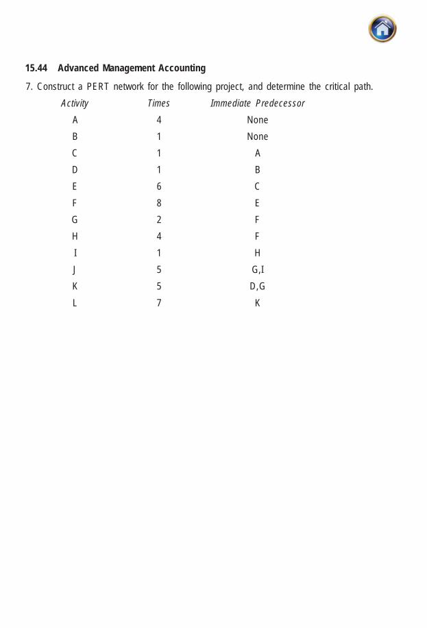
15.44 Advanced Management Accounting
7. Construct a PERT network for the following project, and determine the critical path.
Activity Times Immediate Predecessor
A 4 None
B 1 None
C 1 A
D 1 B
E 6 C
F 8 E
G 2 F
H 4 F
I 1 H
J 5 G,I
K 5 D,G
L 7 K

16Simulation
LEARNING OBJECTIVES :
After studying this chapter, you should be able to :
� explain the term simulation and reasons for using simulation;
� identify the steps in the simulation process;
� review the reasons why simulation may be preferable to other decision models;
� simulate a situation based on real data;
� make useful contribution in (investment decision or capital budgeting) throughsimulation;
� establish how simulation permits study of a system under controlled conditions.
16.1 INTRODUCTION
For various managerial problems discussed so far, we have been able to find a mathematicalsolution. However, in each of these cases the problem (e.g. linear programming or CPM/PERT) was simplified by certain assumptions so that the appropriate mathematicaltechniques could be employed. There are certain managerial situations which are socomplex that mathematical solution is impossible given the current state of the art inmathematics. In many other cases, the solutions which result from simplifying assumptionsare not suitable for the decision makers. In these cases, simulation offers a reasonablealternative.
16.2 WHAT IS SIMULATION?
Simulation is a quantitative procedure which describes a process by developing a model ofthat process and then conducting a series of organised trial and error experiments to predictthe behavior of the process over time. Observing the experiments is much like observingthe process in operation. To find how the real process would react to certain changes, wecan introduce these changes in our model and simulate the reaction of the real process tothem. For example, in designing an airplane, the designer can build a scale model andobserve its behavior in a wind tunnel. In simulation, we build mathematical models whichwe cannot solve and run them on trial data to simulate the behavior of the system.

16.2 Advanced Management Accounting
16.2.1 Steps in the simulation process : All simulations vary in complexity from situationto situation. However, in general, one would have to go through the following steps:-
1. Define the problem or system you intend to simulate.
2. Formulate the model you intend to use.
3. Test the model, compare its behavior with the behavior of the actual problemenvironment.
4. Identify and collect the data needed to test the model.
5. Run the simulation.
6. Analyze the results of the simulation and, if desired, change the solution you areevaluating.
7. Rerun the simulation to test the new solution.
8. Validate the simulation, that is, increase the chances that any inferences you drawabout the real situation from running the simulation will be valid.
It may be noted that the fundamental principle of simulation is to make use of some devicethat can represent the phenomenon of a real-life system to enable us to understand theproperties, behavior and functional characteristics of the system. The device used can beany convenient means-a mathematical formula or a physical model.
The aircraft simulator to train pilots on new models of aircraft represents the use of physicalmodel as a means of experimentation. The mathematical models of real-life situations ininvestment analysis, scheduling or inventory control can be experimented; these are knownas symbolic simulation models. These models can be either deterministic or probabilistic.The deterministic models can provide answers to ‘what if’ type of questions in businessproblems. The probabilistic simulation models deal with random phenomenon and themethod of simulation applied is known as Monte Carlo simulation.
16.3 MONTE CARLO SIMULATION
The Monte Carlo method is the earliest method of simulation; the method employs randomnumbers and is used to solve problems that depend upon probability, where physicalexperimentation is impracticable and the creation of a mathematical formula impossible.It is method of Simulation by the sampling technique. That is, first of all, the probabilitydistribution of the variable under consideration is determined; then a set of random numbersis used to generate a set of values that have the same distributional characteristics as theactual experience it is deviced to simulate. The steps involved in carrying out Monte CarloSimulation are:
(i) Select the measure of effectiveness of the problem, that is, what element is used tomeasure success in improving the system modelled. This is the element one wants tomaximise or minimise. For example, this might be idle time of a service facility, orinventory shortages per period etc.

16.3Simulation
(ii) Identify the variables which influence the measure of effectiveness significantly. Forexample, the number of service facilities in operation or the number of units in inventoryand so on.
(iii) Determine the proper cumulative probability distribution of each variable selected understep (ii). Plot these, with the probability on the vertical axis and the values of variableson horizontal axis.
(iv) Get a set of random numbers.
(v) Consider each random number as a decimal value of the cumulative probabilitydistribution. With the decimal, enter the cumulative distribution plot from the verticalaxis. Project this point horizontally, until it intersects cumulative probability distributioncurve. Then project the point of intersection down into the vertical axis.
(vi) Record the value (or values if several variables are being simulated) generated instep (v) into the formula derived from the chosen measure of effectiveness. Solve andrecord the value. This value is the measure of effectiveness for that simulated value.
(vii)Repeat steps (v) and (vi) until sample is large enough for the satisfaction of the decisionmaker.
In assigning a set of random numbers, we have to decide on the entire range of randomnumbers. If the cumulative probabilities are in two digits the range of random numbers tobe assigned are 00 to 99; and if in three digits, the range is from 000 to 999, and so on.
In view of the enormous computations involved, computer is usually a necessary adjunctthough below we shall deal with quite a few simple simulation problems towards itsexposition.
Example : (For finding the value π experimentally by simulation):
In the figure below is shown the arc of a circle of a unit radius in the first quadrant. Alsoshown is a square OABC of side of one unit.
Fig. 1
A B
y
C
y
xO x
r = 1P

16.4 Advanced Management Accounting
The equation of the circle is given by x2 + y2 = 1. Two* random numbers, each less thanunity (viz., x = 0.1906 and y = 0.3698) are picked up and the point P corresponding to theseis shown plotted. Obviously, if x2 + y2 < 1, P is inside or on the circle but if x2 + y2 > 1, P isbeyond the circle but within the square.
In this manner, hundreds or thousands of pairs of random numbers are picked up and it isascertained if the points corresponding to them fall in/on the arc or beyond the square.Suppose that n out of the total of N points fall in/on the arc.
Now the area enclosed by the arc = π π
4412 = and the area enclosed by the square = 12=1
π /4 π1
4= =nN
orn
N
The experiment value of π is thus obtained. Obviously larger the sample size N, closershall be the true value of π.
This way, the Monte Carlo methods can be applied to solve complex and stochastic/deterministic queuing, inventory control, production scheduling, etc. problems. The methodshave since recently been also applied in moon landing and studying galactic collisions,atomic behavior and in military.
Illustration
Nine villages in a certain administrative area contain 720, 130, 150, 240, 960, 100, 52, 35,532 fields respectively. Make a random selection of six fields using the random numbertables.
Solution
1 2 3 4Village No. No. of Villages Cumulative No. Random nos. fitted
Of Villages against the villageAs per column 3.
1 720 720 0091,06842 130 850 0839,08143 150 10004 240 12405 960 27006 100 23007 52 23528 36 2388 23779 532 2920 2471
* See the Appendix on an excerpt of random nos. at the end of the chapter. How to use it is explained by examplebelow it. However, the nos. we are using have been taken from the other excerpt.

16.5Simulation
The first random no. picked up from the random no. tables is 2377. Since it is immediately< 2388 in Col. 3; it is fitted against village 8 in Col. 4. The next random no. 5997 is > 2920in Col. 4; therefore, it is dropped. In this manner, the following random nos. are, either fittedin Col. 4 or dropped; 8269 (D= drop), 8385 (D), 6198 (D), 0091 (Fl) = fitted against villageno. 1 col. 4) 4829 (D), 3322 (D), 0684 (Fl), 3267 (D), 8209 (D), 5166 (D), 0839 (F2),0814 (F2), 7409 (D), 2471 (F9). We stop here because 6 fields have been selected, twoeach from village nos. I and 2 and one each from village nos. 8 and 9.
Illustration
Frontier Bakery keeps stock of a popular brand of cake. Daily demand based on pastexperience is as given below:-
Experience indicates
Daily demand : 0 15 25 35 45 50
Probability : .01 .15 .20 .50 .12 .02
Consider the following sequence of random numbers:-
R. No. 48, 78, 09, 51, 56, 77, 15, 14, 68, 09
Using the sequence, simulate the demand for the next 10 days.
Find out the stock situation if the owner of the bakery decides to make 35 cakes every day.Also estimate the daily average demand for the cakes on the basis of simulated data.
Solution
According to the given distribution of demand, the random number coding for variousdemand levels is shown in Table below :
Random Number Coding
Demand Probability Cum. Prob. Random nos. fitted
0 0.01 0.0 00
15 0.15 0.16 01-15
25 0.20 0.36 16-35
35 0.50 0.86 36-85
45 0.12 0.98 86-97
50 0.02 1.00 98-99
The simulated demand for the cakes for the next 10 days is given in the Table below. Alsogiven in the table is the stock situation for various days in accordance with the bakerydecision of making 35 cakes per day.

16.6 Advanced Management Accounting
Determination of Demand and Stock Levels
Day Random Number Demand Stock
1 48 35
2 78 35 –
3 09 15 20
4 51 35 20
5 56 35 20
6 77 35 20
7 15 15 40
8 14 15 60
9 68 35 60
10 09 15 80
Expected demand = 270/10 = 27 units per day.
Illustration
A company manufactures around 200 mopeds. Depending upon the availability of rawmaterials and other conditions, the daily production has been varying from 196 mopped to204 mopped, whose probability distribution is as given below:-
Production per day Probability
196 0.05
197 0.09
198 0.12
199 0.14
200 0.20
201 0.15
202 0.11
203 0.08
204 0.06
The finished mopeds are transported in a specially designed three storeyed lorry that canaccommodate only 200 mopped. Using the following 15 random numbers 82, 89, 78, 24,53, 61, 18, 45, 04, 23, 50, 77, 27, 54, 10, simulate the process to find out:
(i) What will be the average number of mopeds waiting in the factory?
(ii) What will be the average number of empty spaces on the lorry?

16.7Simulation
Solution
The random numbers are established as in Table below:
Production Probability Cumulative Random NumberPer day Probability
196 0.05 0.05 00-04197 0.09 0.14 05-13198 0.12 0.26 14-25199 0.14 0.40 26-39200 0.20 0.60 40-59201 0.15 0.75 60-74202 0.11 0.86 75-85203 0.08 0.94 86-93204 0.06 1.00 94-99
Based on the 15 random numbers given we simulate the production per day as above intable 2 below.
Random No. Estimated No. of mopeds waiting No. of emptyProduction spaces in the lorryPer day
Opening Current Current TotalBalance Excess short waiting
produ- produc-ction tion
1 82 202 – 2 – 2 –2 89 203 2 3 – 5 –3 78 202 5 2 – 7 –4 24 198 7 – 2 5 –5 53 200 5 – – 5 –6 61 201 5 1 – 6 –7 18 198 6 – 2 4 –8 45 200 4 – – 4 –9 04 196 4 – 4 0 –10 23 198 0 – 2 0 211 50 200 0 – – – –12 77 202 0 2 – 2 –13 27 199 2 – 1 1 –14 54 200 1 – – 1 –15 10 197 1 – 3 – 2
Total 42 4

16.8 Advanced Management Accounting
Average number of mopeds waiting =42
= 2.8015
Average number of empty spaces in lorry = 4 = 0.26615
(Note : Some of the authors have solved this problem without adjusting excess/short pro-duction. However, we feel that above approach in better.)
Illustration
Ramu and Raju are workers on a two-station assembly line. The distribution of activitytimes at their stations is as follows:–
Time in Time frequency Time frequency
Sec. For Ramu for Raju
10 4 4
20 6 5
30 10 6
40 20 7
50 40 10
60 11 8
70 5 6
80 4 4
(a) Simulate operation of the line for eight times. Use the random numbers given below:
Operation 1 Operation 2
14 61 36 97
01 82 76 41
96 00 55 56
44 03 25 34
(b) Assuming Raju must wait until Ramu completes the first item before starting work, willhe have to wait to process any of the other eight items? Explain your answer, based uponyour simulation.
Solution
Cumulative frequency distribution for Ramu is derived below. Also fitted against it are theeight given random numbers. In parentheses are shown the serial numbers. of randomnumbers.

16.9Simulation
10 4 01(2) 00(7) 03(8)20 1030 20 14(l)40 4050 80 44(4) 61(5)60 91 82(6)70 96 95(3)80 100
Thus the eight times are: 30, 10, 70, 50, 50, 60, 10 and 10 respectively.
Likewise the eight times for Raju are derived from his cumulative distribution below:-
1 2 3 4Frequency Cumulative 2 × col. 3
10 4 4 820 5 9 18 13(7)30 6 15 30 25(4)40 7 22 44 36(1), 34(8)
41(6),50 10 32 64 55(3)60 8 40 80 76(2)70 6 46 9280 4 50 100 97(5)
(Note that cumulative frequency has been multiplied by 2 in Co. 4 in order that all the givenrandom numbers are utilised).
Thus, Raju’s times are 40,60,50,30,80,40,20 and 40 seconds respectively.
Ramu’s and Raju’s times are displayed below to observe for waiting time, if any.
1 2 3 4Ramu Cum. time Raju Raju’s cumulative time
initial with 30 seconds included
30 30 40 7010 40 60 13070 110 50 18050 160 30 21050 210 80 29060 270 40 33010 280 20 35010 290 40 390
Since col. 4 is consistently greater than col. 2 no subsequent waiting is involved.

16.10 Advanced Management Accounting
Illustration
Dr. STRONG is a dentist who schedules all her patients for 30 minutes appointments.Some of the patients take more or less than 30 minutes depending on the type of dentalwork to be done. The following summary shows the various categories of work, theirprobabilities and the time needcd to complete the work :
Category Time required Probability of category
Filling 45 minutes 0.40Crown 60 minutes 0.15Cleaning 15 minutes 0.15Extraction 45 minutes 0.10Checkup 15 minutes 0.20
Simulate the dentist’s clinic for four hours and determine the average waiting time for thepatients as well as the idleness of the doctor. Assume that all the patients show up at theclinic at exactly their scheduled arrival time starting at 8.00 a.m. Use the following randomnumbers for handling the above problem:
40 82 11 34 25 66 17 79SolutionIf the numbers 00-99 are allocated in proportion to the probabilities associated with eachcategory of work, then various kinds of dental work can be sampled, using random numbertable:
Type Probability Random NumbersFilling 0.40 00-39Crown 0.15 40-54Cleaning 0.15 55-69Extraction 0.10 70-79Checkup 0.20 80-99
Using the given random numbers, a work sheet can now be completed as shown on nextpage:
Future Events
Patient Scheduled Arrival R. No. Category Service Time1 8.00 40 Crown 60 minutes2 8.30 82 Checkup 15 minutes3 9.00 11 Filling 45 minutes4 9.30 34 Filling 45 minutes5 10.00 25 Filling 45 minutes6 10.30 66 Cleaning 15 minutes7 11.00 17 Filling 45 minutes8 11.30 79 Extraction 45 minutes

16.11Simulation
Now, let us simulate the dentist’s clinic for four hours starting at 8.00 A.M.
Status
Time Event Number of the patient Patients
Being served (time to go) waiting
8.00 lst patient arrives lst (60) –
8.30 2nd arrives lst (30) 2nd
9.00 lst departs
9.00 3rd arrives 2nd(15) 3rd
9.15 2nd departs 3rd(45)
9.30 4th arrives 3rd (30) 4th
10.00 3rd depart
5th arrives 4th (45) 5th
10.30 6th arrives 4th (15) 5th &6th
10.45 4th departs 5th (45) 6th
11.00 7th arrives 5th (30) 6th & 7th
11.30 5th departs
8th arrives 6th (15) 7th & 8th
11.45 6th departs 7th (45) 8th
12.00 End 7th (30) 8th
12.30 – 8th (45) –
The dentist was not idle during the entire simulated period:
The waiting times for the patients were as follows:
Patient Arrival Service Starts Waiting
(Minutes)
1 8.00 8.00 0
2 8.30 9.00 30
3 9.00 9.15 15
4 9.30 10.00 30
5 10.00 10.45 45
6 10.30 11.30 60
7 11.00 1l.45 45
8 11.30 12.30 60
Total 285
The average waiting time of a patient was = 285
8 = 35.625 minutes.

16.12 Advanced Management Accounting
Illustration
A bakery chain delivers cakes to one of its retail stores each day. The number of cakesdelivered each day is not constant but has the following distribution:-
Cakes delivered per day Probability
10 0.05
11 0.10
12 0.15
13 0.35
14 0.20
15 0.10
16 0.05
The number of customers desiring cakes each day has the distribution:
No. of customers Probability
5 0.10
6 0.15
7 0.20
8 0.40
9 0.10
10 0.05
Finally, the probability that a customer in need of cakes wants 1, 2, or 3 cakes is describedby
Cakes to a customer Probability
1 0.40
2 0.40
3 0.20
Estimate by Monte Carlo methods the average number of cakes left over per day and theaverage number of sales per day owing to lack of cakes. Assume that left over cakes aregiven away at the end of each day.

16.13Simulation
Solution
The first cumulative probability distribution is derived below:
Cumulative probability distribution of cakes delivered per day
Cakes per day Cumulative Ten random
Probability nos. fitted in
10 0.05 .0153(9)
11 0.15 .1342(6)
12 0.30 .2291(4)
13 0.65 .5878(2),.4391(5),.5210(7),.3411(8)
14 0.85 .8136(1),.7923(10).
15 0.95
16 1.00 .9655(3)
Thus, the cakes delivered in each of the 10 days are: 14, 13, 16, 12, 13, 1l, 13, 13, 10, 14.
Likewise the no. of customers per day are derived below from the cumulative probabilitydistribution.
No. of customers Cumulative probability Ten random nos. fitting in
5 0.10 .0906(9)
6 0.25 .2416(4),.1934(10)
7 0.45.3501(l),.3396(3),.2587(5),.3072(6)
8 0.85 .5054(2)
9 0.95 .8511(7), .8698(8)
10 1.00
Thus the number of customers for the ten days are 7, 8, 7, 6, 7, 7, 9, 9, 5, 6, and the totalno. of customers = 71.

16.14 Advanced Management Accounting
Thus cakes delivered per day and the no. of customers per day are laid out below.
Days
1 2 3 4 5 6 7 8 9 10
No. of Customers
desiring cake on nth Day 7 8 7 6 7 7 9 9 5 6
No. of 1
cakes desired 2
by each customer 3
3
2
1
2
No. of cakes wanted 14
No. of cakes delivered 14 13 16 12 13 11 13 13 10 14
Lift overs NIL
Shortage NIL
This table has to be filled in by selecting no. of cakes demanded by each customer fromthe third cumulative distribution derived below. In the first day, there are seven customers.Thus 7 random nos. have been fitted in the cumulative probability distribution below. These,in turn, have been put under day 1 of the above table. The student may fill in the remainingcolumns himself, as an exercise.
Cumulative probability distribution of the no. of cakes wanted by the customers.
(7 random nos. fitted in below give the entries under day of 1 for the above table.)
No. of Cakes Cumulative probability 7 random numbers fitted in for day 1
1 0.40 .23(1), .00(6)
2 0.80 .49(2), .61(5), .48(7)
3 1.00 .82(3), .84(4)
Thus the no. of cakes wanted by the 7 customers in the first day are 1, 2, 3, 3, 2, 1, 2. Theseare entered under day 1. Left-overs and shortages are also computed which may be doneby student for the remaining columns.
16.4 SIMULATION AND INVENTORY CONTROL
The Monte Carlo simulation is widely used to solve inventory problems characterised byuncertainty of demand and lead time. The distribution of demand during the lead time canbe obtained from an empirical analysis of past data or by computer simulation using randomnumbers. The cumulative probability distribution of demand during the lead time is used as

16.15Simulation
a basis to determine the annual inventory costs and stock-out costs for different levels of thesafety stock. The management can experiment the effect of various inventory policies byusing simulation and finally select an optimum inventory policy. The purpose of simulation,as applied to inventory, is to facilitate the management in selecting an inventory policy thatwill result in minimum annual inventory costs-ordering, carrying and stock-out costs. Theapplication of simulation to inventory control is explained below with the help of an example.
The distribution of demand during the lead time and the distribution of the lead time are setout in Tables 1 and 2.
Table 1 : Distribution of Demand during Lead time
Quantity demanded Probabilityduring lead time
0 0.101 0.452 0.303 0.15
Table 2 : Distribution of Lead time
Lead time (weeks) Probability2 0.203 0.654 0.15
Suppose, the management wants to ascertain the annual inventory costs, if they wish toreorder when the quantity on hand is 6 units and order each time a quantity of 12 units.Assume that all orders are delivered for the entire quantity. The cost of ordering isRs. 120, and the cost of holding the inventory in stock is Rs. 5 per unit per week. Further,the management has found that when it runs out-of-stock, it costs Rs. 75 per unit.
Table 5 illustrates the manual simulation for 15 weeks. Before proceeding with simulatingthe demand for each week, we calculate first the cumulative probability and assign randomnumbers for each value of the two variables-demand and lead time. These are set out inTables 3 and 4.
Table 3
Demand Cumulative Random No.s
Probability assigned
0 0.10 00 to 09
1 0.55 10 to 54
2 0.85 55 to 84
3 1.00 85 to 99

16.16 Advanced Management Accounting
Table 4
Lead Title Cumulative Random Nos.Probability assigned
2 0.20 00 to 193 0.85 20 to 844 1.00 85 to 99
We assume that the stock on hand at the start of the simulation process is 10 units. Further,we also assume that all orders are placed at the beginning of the week and all deliveriesagainst orders are received at the beginning of the week.
The simulated demand for work 1 is 1 unit (corresponding to the random number 49 inTable 3), and the closing inventory is 9 units. The inventory-carrying cost works out to9 × 5 = Rs. 45 (Rs. 5 per unit per week). The inventory-carrying costs are calculated for theremaining weeks in the same way. At the end of week 4, the closing inventory is 6 units(reorder point). So an order is placed at the beginning of week 5 for a quantity of 12 units(ordering quantity). The simulated lead time is 3 weeks (corresponding to random number84 in Table 4). This order quantity is, therefore, received at the beginning of week 8. Wenotice from Table 5 that another order is placed at the beginning of week 12, when thestock on hand is 6 units, which is equal to the reorder point. Again, the simulated lead timeis 3 weeks. Before this quantity is received At the beginning of week 15, we find that thequantity available at the beginning of week 14 is 1 unit and the simulated demand for thatweek is 2 units, giving rise to a stock out of 1 unit. The stock-out cost is Rs. 75.
Table 5. Simulation of Demand and Lead Time for 15 weeks.
Week Stock Demand Quantity Stock Inventory Stock out Lead Timeon hand received on hand carrying Quantity Costs Random Leadbeginning Random Quantity end of costs No. Timeof week No. demanded week period
1 10 49 1 – 9 452 9 67 2 – 7 353 7 06 0 – 7 354 7 30 1 – 6 305 6 95 3 – 3 15 84 36 3 01 0 – 3 157 3 10 1 – 2 108 2 70 2 12 12 609 12 80 2 – 10 50
10 10 66 2 – 8 4011 8 69 2 – 6 3012 6 76 2 – 4 20 79 313 4 86 3 – 1 514 1 56 2 – – – 1 7515 – 84 2 12 10 50

16.17Simulation
For the simulated period of 15 weeks, the total inventory costs are:-
Inventory carrying costs = Rs. 440
Ordering costs (2 orders × 20) = Rs. 240
Stock-out costs (1 stock-out) = Rs. 75
Total = Rs. 735
By simulating over a period of 2 to 3 years (i.e. 100 or 150 weeks), we can obtain a moreaccurate picture of the annual inventory costs.
By varying the values of the variables (the ordering quantity and the reorder point), themanagement can find out the effect of such a policy in terms of the annual inventory costs.In other words, simulation permits the management to evaluate the effects of alternateinventory policies. Also, if there is a change in the ordering, stock-out and inventory-carryingcosts, their impact on the annual inventory costs can be determined by using simulation.
16.5 MISCELLANEOUS ILLUSTRATIONS
Illustration
A company manufactures 30 items per day. The sale of these items depends upon demandwhich has the following distribution:
Sales (Units) Probability
27 0.10
28 0.15
29 0.20
30 0.35
31 0.15
32 0. 05
The production cost and sale price of each unit are Rs. 40 and Rs. 50 respectively. Anyunsold product is to be disposed off at a loss of Rs. 15 per unit. There is a penalty of Rs.5 per unit if the demand is not met.
Using the following random numbers estimate total profit / loss for the company for the next10 days: 10, 99, 65, 99, 95, 01, 79, 11, 16, 20
If the company decides to produce 29 items per day, what is the advantage or disadvantageto the company?
Solution
First of all, random numbers 00-99 are allocated in proportion to the probabilities associatedwith the sale of the items as given below:

16.18 Advanced Management Accounting
Sales (units) Probability Cumulative Random numbersprobability assigned
27 0.10 0.10 00-0928 0.15 0.25 10-2429 0.20 0.45 25-4430 0.35 0.80 45-7931 0.15 0.95 80-9432 0.05 1.00 95–99
Let us now simulate the demand for next 10 days using the given number in order toestimate the total profit/loss for the company. Since the production cost of each item is Rs.40 and sale price is Rs. 50, therefore the profit per unit of the sold item will be Rs. 10.There is a loss of Rs. 15 per unit associated with each unsold unit and a penalty of Rs. 5per unit if the demand is not met. Accordingly, the profit / loss for next ten days are calculatedin column (iv ) of the table below if the company manufactures 30 items per day.
(i) (ii) (iii) (iv) (v)Day Random Estimated Profit/Loss per day when Profit/loss per day when
number sale production = 30 items per day production = 29 items per day1 10 28 28 × Rs. 10 – 2 × Rs. 1.5=250 28 × Rs. 10 – 1 × Rs. 15=2652 99 32 30 × Rs. 10 – 2 × Rs.5=290 29 × Rs. 10 – 3 × Rs. 5 = 2753 65 30 30 × Rs. 1 0=300 29 × Rs.10 – 1 × Rs.5=2854 99 32 30 × Rs. 10 – 2 × Rs.5=290 29 × Rs. 10 – 3 × Rs.5=2755 95 32 30 × Rs. 10 – 2 × Rs.5=290 29 × Rs. 10 – 3 × Rs.5=2756 01 27 27 × Rs. 10 – 3 × Rs. 1 5=225 27 × Rs. 10 – 2 × Rs. 5=2407 79 30 30 × Rs.10 = 300 29 × Rs. 10 – 1 × Rs. 5=2858 11 28 28 × Rs. 10 – 2 × Rs. 1 5=250 28 × Rs. 1 0 -1 × Rs. 15=2659 16 28 28 × Rs.10 – 2 × Rs.15=250 28 × Rs.10 - 1× Rs.15= 26510 20 28 28 × Rs. 10 – 2 × Rs. 1 5=250 28 × Rs. 1 0 - 1 × Rs. 1 5=265
Total Profit = Rs.2695 Rs.2695
The total profit for next 10 days will be Rs. 2695 if the company manufactures 30 items per day.In case, the company decides to produce 29 items per day, then the profit of the company fornext 10 days is calculated in column (v) of the above table. It is evident from this table that thereis no additional profit or loss if the production is reduced to 29 items per day since the total profitremains unchanged i.e. Rs. 2695.
Illustration
An Investment Corporation wants to study the investment projects based on three factors : marketdemand in units, price per unit minus cost per unit, and the investment required. These factorsare felt to be independent of each other. In analysing a new consumer product, the corporationestimates the following probability distributions:

16.19Simulation
Annual (Price-Cost) Probability Investment Required
demand per unit Rs. ProbabilityUnits Probability Rs.25,000 0.05 3.00 0.10 27,50,000 0.2530,000 0.10 5.00 0.20 30,00,000 0.5035,000 0.20 7.00 0.40 35,00,000 0.2540,000 0.30 9.00 0.2045,000 0.20 10.00 0.1050,000 0.1055,000 0.05
Using simulation process, repeat the trial 10 times, compute the return on investment for eachtrial, taking these three factors into account. Approximately, what is the most likely return? Usethe following random numbers for annual demand, (price-cost) and the investment required:28, 57, 60, 17, 64, 20, 27, 58, 61, 30; 19, 07, 90, 02 57,
28, 29, 83, 58, 41, 18, 67, 16, 71, 43, 68, 47, 24, 19, 97
Solution
The yearly return can be determined by the formula:
Return (R) = (Price – Cost) Number of units demanded
Investment
×
The results of the simulation are shown in the table given below:
Trials Random Simulated Random Simulated Random Simulated SimulatedNumber of Demand Number Profit number investment Return (%)Demand (‘000) for profit for (‘000) Demand ×
(Price-Cost) investment Profit perper unit Investment
1 28 35 19 5.00 18 2750 6.362 57 40 07 3.00 67 3000 4.003 60 40 90 10.00 16 2750 14.554 17 35 02 3.00 71 3000 3.505 64 40 57 7.00 43 3000 9.336 20 35 28 5.00 68 3000 5.837 27 35 29 5.00 47 3000 5.838 58 40 83 9.00 24 2750 13.109 61 40 58 7.00 19 2750 10.1810 30 35 41 7.00 97 3500 7.00

16.20 Advanced Management Accounting
Result: Above table shows that the highest likely return is 14.6% which is corresponding tothe annual demand of 40,000 units resulting a profit of Rs. 10 per unit and the requiredinvestment will be Rs. 27,50,000.
IllustrationThe occurrence of rain in a city on a day is dependent upon whether or not it rained on theprevious day. If it rained on the previous day, the rain distribution is given by:
Event Probability
No rain 0.50
1 cm. rain 0.25
2 cm. rain 0.15
3 cm. rain 0.05
4 cm. rain 0.03
5 cm. rain 0.02
If it did not rain the previous day, the rain distribution is given by:
Event Probability
No rain 0.75
1 cm. rain 0.15
2 cm. rain 0.06
3 cm. rain 0.04
Simulate the city’s weather for 10 days and determine by simulation the total days without rainas well as the total rainfall during the period. Use the following random numbers:
67 63 39 55 29 78 70 06 78 76
for simulation. Assume that for the first day of the simulation it had not rained the day before.
SolutionThe numbers 00-99 are allocated in proportion to the probabilities associated with each event.If it rained on the previous day, the rain distribution and the random number allocation aregiven below:
Event Probability Cumulative Random
Probability numbers
assigned
No rain 0.50 0.50 00-49
1 cm. rain 0.25 0.75 50-74
2 cm. rain 0.15 0.90 75-89
3 cm. rain 0.05 0.95 90-94
4 cm. rain 0.03 0.98 95-97
5 cm. rain 0.02 1.00 98-99
Table I : Rain on previous day

16.21Simulation
Similarly, if it did not rain the previous day, the necessary distribution and the randomnumber allocation is given below:
Event Probability Cumulative Random
Probability numbers
assigned
No rain 0.75 0.75 00-74
1 cm. rain 0.15 0.90 75-89
2 cm. rain 0.06 0.96 90-95
3 cm. rain 0.04 1.00 96-99
Table 2: No rain on previous day
Let us now simulate tile rain fall for 10 days using the given random numbers. For tile firstday it is assumed that it had not rained the day before:
Day Random Event
Numbers
1 67 No rain (from table 2)
2 63 No rain (from table 2)
3 39 No rain (from table 2)
4 55 No rain (from table 2)
5 29 No rain (from table 2)
6 78 1 cm. rain (from table 2)
7 70 1 cm. rain (from table 1)
8 06 No rain (from table 1)
9 78 1 cm. rain (from table 2)
10 76 2 cm. rain (from table 1)
Hence, during the simulated period, it did not rain on 6 days out of 10 days. The total rainfell during the period was 5 cm.
Illustration
The output of a production line is checked by an inspector for one or more of three differenttypes of defects, called defects A, B and C. If defect A occurs, the item is scrapped . If defectB or C occurs, the item must be reworked. The time required to rework a B defect is 15minutes and the time required to rework a C defect is 30 minutes. The probabilities of anA, B and C defects are .1 5, .20 and .10 respectively. For ten items coming off the assembly

16.22 Advanced Management Accounting
line, determine tile number of items without any defects, the number scrapped and thetotal minutes of rework time. Use the following random numbers,
RN for defect A
48 55 9 1 40 93 01 83 63 47 52
RN for defect B
47 36 57 04 79 55 10 13 57 09
RN for defect C
82 95 1 8 96 20 84 56 11 52 03
Solution
The probabilities of occurrence of A, B and C defects are 0.15, 0.20 and 0.I0 respectively. So,tile numbers 00-99 are allocated in proportion to the probabilities associated with each of thethree defects
Defect A Defect B Defect C
Exists Random Exists ? Random Exists ? Random
numbers numbers numbers
assigned assigned assigned
Yes 00-14 Yes 00-19 Yes 00-09
No 15-99 No 20-99 No 10-99
Let us now simulate the output of the assembly line for 10 items using the given random numbersin order to determine the number of items without any defect, the number of items scrapped andthe total minutes of rework time required:
Item RN for RN for RN for Whether Rework Remarks
No. defect A defect B defect C any defect time (in
exists minutes)
1 48 47 82 None – –
2 55 36 95 None – –
3 91 57 18 None – –
4 40 04 96 B 15 –
5 93 79 20 None – –
6 01 55 84 A – Scrap
7 83 10 56 B 15 –
8 63 13 11 B 15 –
9 47 57 52 None – –
10 52 09 03 B,C 15+30=45 –

16.23Simulation
During the simulated period, 5 out of the ten items had no defects, one item was scrapped and90 minutes of total rework time was required by 3 items.
Illustration
The management of ABC company is considering the question of marketing a new product.The fixed cost required in the project is Rs. 4,000. Three factors are uncertain viz. the sellingprice, variable cost and the annual sales volume. The product has a life of only one year. Themanagement has the data on these three factors as under:
Selling Probability Variable Probability Sales ProbabilityPrice Cost volumeRs. Rs. (Units)3 0.2 1 0.3 2,000 0.34 0.5 2 0.6 3,000 0.35 0.3 3 0.1 5,000 0.4
Consider the following sequence of thirty random numbers:
81 32 60 04 46 31 67 25 24 10 40 02 39 68
08 59 66 90 12 64 79 31 86 68 82 89 25 1198 16
Using the sequence (First 3 random numbers for the first trial, etc.) simulate the average profit forthe above project on the basis of 10 trials.
Solution
First of all, random numbers 00–99 are allocated in proportion to the probabilities associatedwith each of the three variables as given under:
Selling Price Probabilities Cumulative Random numbersRs. Probabilities assigned
3 0.2 0.2 00-194 0.5 0.7 20-695 0.3 1.0 70-99Variable cost (Rs.)
1 0.3 0.3 00-292 0.6 0.9 30-893 0.1 1.0 90-99Sales Volumes (Units)2,000 0.3 0.3 00-293,000 0.3 0.6 30-595,000 0.4 1.0 60-99

16.24 Advanced Management Accounting
Let us now simulate the output of ten trials using the given random numbers in order to find theaverage profit for the project:
S. No. Random Selling Random Variable Random Sales Volume
No. Price (Rs.) No. Cost (Rs.) No. (‘000 units’)
1 81 5 32 2 60 5
2 04 3 46 2 31 3
3 67 4 25 1 24 2
4 10 3 40 2 02 2
5 39 4 68 2 08 2
6 59 4 66 2 90 5
7 12 3 64 2 79 5
8 31 4 86 2 68 5
9 82 5 89 2 25 2
10 11 3 98 3 16 2
Profit = (Selling Price – Variable cost) × Sales Volume – Fixed cost.
Simulated profit in ten trials would be as follows:
S.No. Profit1 (Rs.5 – Rs.2) × 5,000 units – Rs. 4,000 = Rs. 11,0002 (Rs.3 – Rs. 2) × 3,000 units – Rs. 4,000 = Rs. – 1,0003 (Rs. 4 – Re. 1) × 2,000 units – Rs. 4,000 = Rs. 2,0004 (Rs.3 – Rs. 2) × 2,000 units – Rs. 4,000 = Rs. – 2,0005 (Rs.4 – Rs. 2) × 2,000 units – Rs. 4,000 = 06 (Rs.4 – Rs. 2) × 5,000 units – Rs. 4,000 = Rs. 6,0007 (Rs.3 – Rs. 2) × 5,000 units – Rs. 4,000 = Rs. 1,0008 (Rs.4 – Rs. 2) × 5,000 units – Rs. 4,000 = Rs. 6,0009 (Rs. 5 – Rs. 2) × 2,000 units – Rs. 4,000 = Rs. 2,00010 (Rs.3 – Rs. 3) × 2,000 units – Rs. 4,000 = Rs.-4,000
Total Rs.2 1,000
Therefore average profit per trial = Rs. 21,000
10Rs. 2,100=
Example on the use of random number table. Suppose we want five 3-digit random nos.We can enter any where in the table e.g. the last column, first 3 digits of 5 consecutive nosgive us the answers : 413, l72, 207, 511, l72. Thus we can enter the table randomly but thenon proceed serially.

16.25Simulation
16.6 RANDOM NUMBERS TABLE8481 5016 0080 4376 2579 8293 5950 1048 0650 41350744 3447 6173 3288 6378 6704 0966 9986 5202 17285558 7239 2976 4836 6134 5120 1541 6514 3581 20799371 1463 2164 2301 3142 3866 8707 9980 2011 51113033 1660 6365 9054 1155 8844 4085 9589 2924 17251053 7320 6532 7214 8972 6466 1217 0100 1458 94164389 3504 4086 9434 0136 5695 6876 7937 5476 33962158 8854 9534 1196 4941 2697 7497 1149 1952 34826749 3676 4943 1406 8614 2060 6433 1660 8875 31942878 3447 4804 6761 5309 0636 0522 2004 3207 46840591 6549 2206 6185 6188 2649 2389 9483 0924 13891025 3438 0546 2545 1089 1280 6701 9742 3453 55734244 9217 1628 4524 0163 9895 9586 2083 8459 06441331 9032 1388 5661 0472 7128 1902 0343 7724 05288853 3490 2589 8744 1221 4667 8396 4779 9937 72065059 4192 6331 5485 5922 0982 9390 8993 3621 26020821 4340 3194 0118 4773 8668 1891 7989 9190 22965262 1746 7108 6496 2570 4243 5029 8949 4989 50081210 1858 9365 6562 0269 9923 1796 6626 8591 19903642 6629 5775 3219 8801 4047 6861 0765 2379 34949598 5322 3747 0363 5995 5504 6804 7033 0957 95563894 3173 2853 9312 2498 8878 4956 8748 6247 66733603 3011 6762 0848 8316 3485 6388 8925 3790 08981121 2978 6313 5857 8457 1395 7240 8630 3895 63481930 4583 4227 4120 6893 7005 2264 6067 5627 79856309 9158 2830 3262 9809 4606 8669 1154 5841 76954460 3143 5383 0327 9668 1697 8335 0860 2188 19088371 5095 7273 1866 4193 4163 2035 2812 4996 71429397 5540 9298 9076 1299 0669 0088 1809 0631 31629304 1468 4013 7465 0861 6787 3581 7977 8409 47085606 2435 8546 3209 4802 6690 8527 2210 6706 19306693 8333 082 7546 2910 8553 8725 1237 4423 15700556 7715 8994 4245 1540 8150 3889 5273 6977 27036973 9299 4959 7146 1426 7086 8743 6982 5547 33944920 1223 5208 6661 4907 1102 0501 3625 8513 31920132 0098 8241 0858 7627 4174 1170 3142 2455 48914051 3101 9854 4488 6931 3266 3147 2500 8011 88480267 5612 5504 7917 7928 8034 9989 4353 2675 94970609 9469 3149 4086 8911 8547 3518 9349 1836 05482593 1666 5750 5105 4287 4380 7860 7792 1625 76598812 9491 2602 4100 4962 1037 9778 1778 4223 31933540 5985 0019 7155 1471 185l 8682 9957 3772 47069535 5375 1239 1624 5378 6803 7177 7911 4660 56693174 7677 8282 6669 5879 7874 9931 6581 9784 26078864 4760 1129 6205 4949 4205 0222 7479 6470 81945245 7341 0593 5656 6799 3071 1751 4339 5630 94965468 6038 4511 1440 2135 5777 9903 1048 6726 86023951 7928 6818 4161 4840 1392 1323 5014 7538 98547319 4064 4024 5401 2834 7518 3978 3742 1005 46195892 8731 6269 5189 2071 4084 9789 3620 9819 4548

16.26 Advanced Management Accounting
(ii) What will be the average number of empty spaces on the lorry ?
l l l
SELF-EXAMINATION QUESTIONS
1. Define a Simulation model. Distinguish between deterministic and stochastic simulationmodel.
2. Discuss Monte Carlo simulation. Illustrate how would you use it in situations of
(i) Queuing and (ii) Inventory Control.
3. Explain in being advantages and disadvantages of using simulation technique.
4. A retailer deals in a perishable commodity. The daily demand and supply are variables. Thedata for the past 500 days show the following demand and supply.
Supply DemandAvailability (kg) No. of days Demand (kg) No. of days
10 40 10 5020 50 20 11030 190 30 20040 150 40 10050 70 50 40
The retailer buys the commodity at Rs. 20 per kg and sells it at Rs. 30 per kg. Any commodityremains at the end of the day, has no saleable value. Moreover, the loss (unearned profit) onany unsatisfied demand is Rs. 8 per kg. Given the following pair of random numbers, simulate6 days sales, demand and profit.
(31,18); (63,84); (15,79); (07,32); (43,75); (81,27)
The first random number in the pair is for supply and the second random number is fordemand viz. in the first pair (31,18) use 31 to simulate supply and 18 to simulate demand.
5. A company manufactures around 200 mopeds. Depending upon the availability of rawmaterials and other conditions, the daily production has been varying from 196 mopeds to204 mopeds whose probability distribution is as given below :
Production per day Probability
196 0.05197 0.09198 0.12199 0.14200 0.20201 0.15202 0.11203 0.08204 0.06

16.27Simulation
The finished mopeds are transported in a specially designed three storeyed lorry that canaccommodate only 200 mopeds. Using the following 15 random numbers 82, 89, 78, 24,53, 61, 18, 45, 04, 23, 50, 77, 27, 54, 10 simulate the process to find out :
(i) What will be the average number of mopeds, waiting in the factory ?
(ii) What will be the average number of empty spaces on the lorry ?

17Learning Curve Theory
LEARNING OBJECTIVES :
After studying this unit, you will be able to :
� Understand, visualize and explain learning curve phenomenon.
� Measure how in some industries and in some situations the incremental cost per unit ofoutput continues to fall for each extra unit produced
� Understand how the percentage learning rate applies to the doubling of output
� Know that cumulative average time means the average time per unit for all units producedso far back to and including the first unit produced.
� Successfully use learning curve theory in such situations as pricing decisions, workscheduling and standard setting
� Describe and identify the situations where learn effect can be incorporated
� Calculate average hours/cost per unit of cumulative productions and incremental hours/cost per order using the learning curve
17.1 INTRODUCTION
Learning is the process by which an individual acquires skill, knowledge and ability. When a newproduct or process is started, performance of worker is not at its best and learning phenomenontakes place. As the experience is gained, the performance of worker improves, time taken perunit reduces and thus his productivity goes up. This improvement in productivity of workers is dueto learning effect. Cost predictions especially those relating to direct labour must allow for theeffect of learning process. This technique is a mathematical technique. It is a graphical tech-nique used widely to predict cost. Learning curve is a geometrical progression, which revealsthat there is steadily decreasing cost for the accomplishment of a given repetitive operation, asthe identical operation is increasingly repeated. The amount of decrease will be less and lesswith each successive unit produced. The slope of the decision curve is expressed as a percent-age. The other names given to learning curve are Experience curve, Improvement curve andProgress curve. It is essentially a measure of the experience gained in production of an article byan organisation. As more units are produced, people involved in production become more effi-cient than before. Each additional unit takes less time to produce. The amount of improvement

17.2 Advanced Management Accounting
or experience gained is reflected in a decrease in man-hours or cost. The application of learningcurve can be extended to commercial and industrial activities as well as defence production.
The learning effect exists during a worker’s start up or familiarization period on a particular job.After the limits of experimental learning are reached, productivity tends to stabilise and no furtherimprovement is possible. The rate at which learning occurs is influenced by many factors includ-ing the relative unfamiliarity of workers with the task, the relative novelty and uniqueness of thejob, the complexity of the process, the impact of incentive plans, supervision, etc.
17.2 DISTINCTIVE FEATURES OF LEARNING CURVE THEORY IN MANUFACTURINGENVIRONMENT
The Theory of learning curve was first introduced by T.P. Wright of Curtiss—Wright, Buffalo,U.S.A. engaged in production of airframes. As the production quantity of a given item doubled, thecost of that item decrease at a fixed rate. This phenomenon is the basic premise on which thetheory of learning curve has been formulated. The key words, ‘doubled’ and ‘rate’ are importantas the quantity produced doubles, the absolute amount of cost increase will be successivelysmaller but the rate of decrease will remain fixed. This is the essence of the learning curve theoryand it occurs due to following distinctive features of manufacturing environment :
(i) Better tooling methods are developed and used;
(ii) More productive equipments are designed and used to make the product;
(iii) Designed bugs are detected and corrected;
(iv) Engineering changes decrease over the time. Designed engineering are prompted to achievebetter design for reducing material and labour cost.
(v) Earlier teething problems are overcome. As the product involves monthly, management isprompted to strive for better planning and better management.
(vi) Rejections and rework tend to diminish over time.
There happen a significant influence of all these features on labour as the quantity producedincreases and the cost per unit drops. The reasons for this are that each unit will entail : (a) lesslabour; (b) less material; (c) more units produced from the same equipments; (d) cost of fewerdelays and less loss time. Every Time Study engineer or industrial engineer experienced in workmeasurement has seen this phenomenon happening. Learning curve applications are fast grow-ing with time in manufacturing environment. A company should never blindly adopt anothercompany's learning curve. The product approach for a company should be to develop knowl-edge of its own learning preference in its plant.
17.3. THE LEARNING CURVE RATIO
In the initial stage of a new product or a new process, the learning effect pattern is so regular thatthe rate of decline established at the outset can be used to predict labour cost well in advance.The effect of experience on cost is summaries in the learning ratio or improvement ratio :
Learning Curve Ratio = unitsNfirstofcostlabourAverageunits2NfirstofcostlabourAverage

17.3Learning Curve Theory
If the average labour cost for the first 500 units of a product is Rs. 25 and the average labour costof first 1,000 units is Rs. 20, the learning ratio will be determined as follow :
Learning curve ratio = 25Rs.
20Rs. × 100 or 80%
This learning curve ratio of 80% means that every time output doubles, the average cost declinesto 80% of the previous amount. Since the average cost per unit of 1,000 units is Rs. 20, theaverage cost of first 2,000 units is likely to be 80% of this, i.e., Rs. 16 per unit. The amount ofproduction improvement in the manufacture of an article will determine the percentage of thelearning curve. The effect of learning can be presented clearly in a diagram drawn known aslearning curve. The units chosen in the progression must always have a ratio of two (Unit 2 to unit1, unit 50 to unit 25, unit 300 to unit 150, etc.). An 80% leaning curve is drawn using the followingdata.
Incremental Cumulative Average time Cumulative
quantity quantity per unit time taken
(1) (2) (3) (4) (5)
1 1 100 100
1 2100
80)(100 ×80 160
2 4100
80)(80 ×64 256
4 8100
80)(64 ×51 408
8 16100
80)(5 ×141 656
| | | | | | | | | | | | | | | | |0 1 2 3 4 5 6 7 8 9 10 11 12 13 14 15 16
100
80
60
40
20
0
Y
X
LEARNING PHASE
STEADY SUTEPHASE
CUMULATIVE OUTPUT
CU
MU
LA
TIV
E A
VE
RA
GE
PE
R U
NIT

17.4 Advanced Management Accounting
Learning Curve
Columns (2) and (4) have been used for drawing the learning curve. Last column is not used indrawing the 80 per cent learning curve. This column shows how the cumulative time consump-tion will increase with decrease in cumulative average per unit. Cumulative quantity is plotted onX-axis and cumulative average time consumption per unit is plotted on Y-axis. After the learningeffect phase is over, steady-state phase will start. Learning effect advantage will not be there issteady-state phase, when the product or the process gets well stabilised.
17.4 LEARNING CURVE EQUATION
Mathematicians have been able to express relationship in equations. The basic equation
Yx = KXs ...(1)
where,
X is the cumulative number of units or lots produced
Y is the cumulative average unit cost of those units X or lots.
K is the average cost of the first unit or lot
s is the improvement exponent or the learning coefficient or the index of learning which iscalculated as follows :
s = 2ofarithmlogratiolearningofarithmlog
Learning curve equation Yx = KXs becomes a linear equation when it is written in its logarithmicform :
log Yx = log K + s log X ...(2)
Each of the above two equations defines cumulative average cost. Either of them can be con-verted to a formula for the total labour cost of all units produced up to a given point. Total costunder equation I can be found out by the following formula :
Total cost = XYx = KXs = KXs+1 ...(3)
17.5 LEARNING CURVE APPLICATION
Knowledge of learning curve can be useful both in planning and control. Standard cost for newoperations should be revised frequently to reflect the anticipated learning pattern. Its main usesare summarised below :
17.5.1 Helps to analyse CVP Relationship during familiarisation phase : Learning curvehelps to analyse cost-volume-profit relationship during familiarisation phase of product or pro-cess and thus it is very useful for cost estimates. Learning curve is of immense value as a tool forforecasting.
Illustration
XYZ Co., has observed that a 90% learning curve ratio applies to all labour related costs eachtime a new model enters production. It is anticipated that 320 units will be manufactured during

17.5Learning Curve Theory
1999. Direct labour cost for the first lot of 10 units amounts to 1,000 hours at Rs. 8 per hour.Variable overhead cost is assigned to products at the rate of Rs. 2 per direct labour hour. You arerequired to determine :
(i) Total labour and labour-related costs to manufacture 320 units of output.
(ii) Average cost of (a) the first 40 units produced (b) the first 80 units, (c) the first 100 units.
(iii) Incremental cost of (a) units 41–80 and (b) units 101–200.
Solution
Table showing cost projections based on 90 per cent learning curve.
Incremental Cumulative Average Cumulative Incremental
quantity quantity time per unit time taken hours
10 10 100 1,000 —
10 20 90 1,800 800
20 40 81 3,240 1,400
40 80 72.9 5,832 2,592
80 160 65.61 10,497.6 4,665.6
160 320 59.049 18,895.68 8,398.08
Following cost information can be derived from the data given in the above table :
(i) Total cost of 320 units = 18,895.68 × Rs. 10 = Rs. 1,88,956.80
(ii) Average cost of first 40 units = 81 × Rs. 10 = Rs. 810 per unit.
Average cost of first 80 units = 72.9 × Rs. 10 or Rs. 729 per unit.
(iii) Incremental cost of units 41 – 80 = 2592 × Rs. 10 or Rs. 25,920.
The basic learning curve formula must be used to derive the average cost of the first 100 unitsand the incremental cost of units 101 – 200.
We know that Yx = KXs
The first production lot contained 10 units. K = 1,000 hrs. (time taken for the first lot) and X = 10(the number of lots needed to produce 100 units).
Taking the logarithm of the above relation, we get
log Y10 = log 1000 + (–0.1518 log 10)
= 3.0 – 0.1518
= 2.8482
Y10 = 705

17.6 Advanced Management Accounting
Y10 means that average processing time for the first 10 lots of output was 705 hours per lot. Eachlot includes 10 units of output. Therefore, average processing time for each of the first 100 unitsis 70.5 hours. The labour rate is Rs. 10 per hour. Therefore, the average cost of the first 100 unitswas Rs. 705 per unit. The incremental cost of units 101 – 200 corresponds to the incrementalcost of lots 11 – 20. This is equal to the total cost of first 20 lots minus the total cost of the first 10lots.
Y10 = 705
Y10 = (1000) (20 – 0.1518) = 634.5
Time for first 20 lots = 20(634.5) = 12,690 hours
Time of first 10 lots = 10 (705) = 7,050 hours
5,640 hours
This means that incremental cost of lots 11 – 20 will be :
(5,640 hrs. × Rs. 10) = Rs. 56,400
17.5.2 Helps in budgeting and profit planning : Incorporation of the learning curve intro-duces new complexity and sophistication in the process of budgeting and profit planning. Budgetexecutive should select those costs which reflect learning effect and then he should be able toincorporate this effect in process of developing budgets or in the exercises relating to projectplanning.
17.5.3 Helps in pricing : The use of cost data adjusted for learning effect helps in developmentof advantageous pricing policy. Suppose, firm A is preparing a bid to produce 220 MW turboset.Hitherto, company had produced a set of 100 MW only. There is a strong possibility of productionover-run. Firm A is competing with Firm B. Firm A is not aware of the learning effect, while FirmB is aware of the learning effect. In this situation, Firm B will definitely go away with the contract.
17.5.4 Design makers : It helps design engineers in making decisions based upon expected(predictable from past experience) rates of improvement.
17.5.5 Helps in negotiations : It is very helpful to Government in negotiations about the con-tracts. Government receives full advantage of the decreasing unit cost in establishing the con-tract price.
17.5.6 Helps in setting standards : The learning curve is extremely useful in setting standardsin learning phase.
17.6 LIMITATIONS OF LEARNING CURVE THEORY
Following limitations of learning curve must be kept in view :
1. All activities of a firm are not subject to learning effect. Following types of activities aresubject to learning effect :
(a) Those, that have not been performed in this present operational mode.

17.7Learning Curve Theory
(b) Those which are being performed by new workmen, new employees or others notfamiliar with the particular activity. In contrast, activities being performed by experi-enced workmen, who are thoroughly familiar with those activities will not be subject tolearning effect.
(c) Those involving utilization of material not used by firm so far.
2. It is correct that learning effect does take place and average time taken is likely to reduce.But in practice it is highly unlikely that there will be a regular consistent rate of decrease, asexemplified earlier. Therefore any cost predictions based on covernational learning curvesshould be viewed with caution.
3. Considerable difficulty arises in obtaining valid data, that will form basis for computation oflearning effect.
4. Even slight change in circumstances quickly renders the learning curve obsolete. While theregularity of conventional learning curves can be questioned, it would be wrong to ignorelearning effect altogether in predicting future costs for decision purposes.
Illustration
Illustrate the use of leaning curves for calculating the expected average unit cost of making.
(a) 4 machines; (b) 8 machines
Using the data below :
Data :
Direct labour needed to make first machine 1,000 hours
Learning curve = 90%
Direct labour cost Rs. 15/per hour
Direct materials cost Rs. 1,50,000
Fixed cost for either size orders — Rs. 60,000.
Solution
Learning curve (90%) for calculating the expected average unit cost
Cumulative Cum. Avg. Cum. Avg. Materials Overheads Total
order size hours labour cost
@ Rs. 15 per hr.
1 1,000 Rs. 15,000 — — —
2 (90% of 1,000) = 900 13,500 — — —
(a) 4 (90% of 900) = 810 12,150 1,50,000 60,000 2,22,150
(b) 8 (90% of 810) = 729 10,935 1,50,000 30,000 1,90,935

17.8 Advanced Management Accounting
Illustration
XYZ & Co. has given the following data :
80% Average – Time Curve
Cumulative Average Total Marginal
Units (x) Hours Hours Hours
1 100 100 100
2 80 160 60
3 ? ? ?
4 64 256 ?
Required : Fill in the blanks
Solution
We know that : Y = axb
where, Y = average time per unit
a = total time for the first unit
x = the cumulative number of units manufactured.
b = the learning index
The learning coefficient, b, is determined as follows :
b = 2log
)decrease%1(log − = 2log
)20.01(log − = 2log
80.0log =
3010.0
1090309.9 − = – 0.322
By inserting the proper values into the equation, average time for any given number of units canbe computed. For three cumulative units, we find that
Y = 100 (3)–.322 = 100. *322.3
1
= 100.4244.1
1 = 100 (.7020) or 70.2
*Log 3 = 0.47712
0.32349
0.15363 Antilog = 1.4244

17.9Learning Curve Theory
Now it is possible to complete the table :
80% Average-Time Curve
Cumulative Average Total Marginal
Units Time Time Time
1 100 100 100 (100 – 0)
2 80 160 (80 × 2) 60 (160 – 100)
3 70.2 210.6 (70.2 × 3) 50.6 (210.6 – 160)
4 64 256 (64 × 4) 45.4 (256 – 210.6)
Each of the values in the table can be determined by means of the formulas :
Units Average time = axb
1 100 (1)–.322 = 100. 322.1
1 = 100
2 100 (2)–.322 = 100. 322.2
1 = 80
3 100 (3)–.322 = 100. 322.3
1 = 70.2
4 100 (4)–.322 = 100. 322.4
1 = 64
Units Total Time = axb+1
1 100 (1)–.322 + 1 = 100 (1).678 = 100
2 100 (2)–.322 + 1 = 100 (2).678 = 160
3 100 (3)–.322 + 1 = 800 (3).678 = 210.6
4 100 (4)–.322 + 1 = 100 (4).678 = 256
Marginal Time = a(b + 1)xb
Units Formula (continuous) (From table above)
1 100 (– .322 + 1) (1)–.322 = 100 (.678) 1 ÷ 1.322 = 67.8 100
2 100 (– .322 + 1) (2)–.322 = 100 (.678) 1 ÷ 2.322 = 54.2 60
3 100 (– .322 + 1) (3)–.322 = 100 (.678) 1 ÷ 3.322 = 47.6 50.6
4 100 (– .322 + 1) (4)–.322 = 100 (.678) 1 ÷ 4.322 = 43.4 45.4

17.10 Advanced Management Accounting
Illustration
A customer has asked your company to prepare a bid on supplying 800 units of a new product.Production will be in batches of 100 units. You estimate that costs for the first batch of 100 unitswill average Rs. 100 a unit. You also expect that a 90% learning curve will apply to the cumulativelabour cost on this contract.
Required : (a) Prepare an estimate of the labour costs of fulfilling this contract.
(b) Estimate the incremental labour cost of extending the production run to produce an additional800 units.
(c) Estimate the incremental labour cost of extending the production run from 800 units to 900units.
Solution
(a) Average cost decreases by 10 per cent every time when the cumulative production doubles.
Therefore,
Average cost of first 200 units = 0.9 × Avg. cost of 100 units
Average cost of first 400 units = 0.9 × Avg. cost of 200 units
Average cost of first 800 units = 0.9 × Avg. cost of 400 units
Combining these, we find that average cost of the first 800 units
= 0.9 × 0.9 × 0.9 × Rs.100 = Rs. 72.90
Total cost = 800 × Rs. 72.90 = Rs. 58,320
(b) Average cost of the first 1,600 units = 0.9 × Rs. 72.9 = Rs. 65.61
∴ Total cost of 1,600 units = 1,600 × Rs. 65.61 = Rs. 1,04,976
Additional cost of 2nd 800 units
= Rs. 1,04,976 – Rs. 58,320 = Rs. 46,656 or Rs. 58.32 per unit
(c) Because this increase will not increase cumulative production to twice of some figurewe already have, formula has to be used :
Y = axb where b = .0458 ÷ 0.301 = – 0.15216
log ax cost = log 10,000 – 0.15216 log 9
= 4 – 0.1452 = 3.8548
Average cost = Rs. 71.5833 per unit
Total cost = 900 × 71.5833 = Rs. 64,425
Incremental cost = Rs. 64,425 – Rs. 58,320 = Rs. 6,105 or Rs. 61.50 per unit.

17.11Learning Curve Theory
SUMMARY
• Learning Curve Effect applies only to direct labour costs and those variable overheads,which are direct function of labour hours of input. It does not apply to material costs, non-variable costs or items which vary with output.
• Incremental hours cannot be directly determined from the learning curve graph or formula,as the results are expressed in terms of cumulative average hours.
SELF-EXAMINATION QUESTIONS
1. What is learning curve. How the learning curve ratio to calculated ?
2. Explain the application of learning curve in business situations.

18Testing of Hypothesis
18.1 INTRODUCTION
The estimation of population parameters and the testing of hypothesis concerning thoseparameters are similar techniques, but at the same time there are major difference in theinterpretation of results arising from each method. When we are concerned with measurement,say, of expenditure on entertainment, the appropriate methods will be the process of elimination.Hypotheses using is very helpful in examining the validity or otherwise of theories such aswage increase leads to rising prices, advertisements leads to increase amount of sales.
18.2 CONCEPT OF HYPOTHESIS : Any statement or question about a statistical populationon the values of its parameters is called a statistical hypothesis. The procedure whichenables us to examine whether a certain hypotheses is true or not is called testing ofhypothesis. For this purpose, we have to collect relevant information, and process it usingstatistical techniques and then test the above statement. In general formulation of hypothesisis generally concerned with the causes of a certain phenomenon or a relationship betweentwo or more variables under estimation.
18.2.1 Concept of Null hypothesis: A null hypothesis can be defined as a statisticalhypothesis which states that there are no differences between the observed and expecteddata. It is a statement about a population parameter and the test is used to decide whetheror not to accept the hypothesis. A null hypothesis is denoted by H
0 is always one of status
quo or no difference. When the statement of the null hypothesis is false, some thing elsemust be true. In view of this probability, when ever a null hypothesis is specified an alternativehypothesis denoted by H
1 should be mentioned. H
1 is the opposite statement of H
0. So when
one hypothesis is accepted, it implies rejection of the other.
18.2.2 Level of significance and critical region:
The decision about rejection or acceptance of the null hypotheses is based on probabilityconcept. Assuming the null hypothesis to be true we calculate the probabilities of obtaininga different equal to or greater than the observed difference. If this probability is found to besmall say less than 0.05, then conclusion is that the observed value of the statistic is ratherunusual and has been arisen because the underlying assumption (i.e. null hypothesis) isnot true. In this case, we conclude that the observed difference is significant at 5% level ofsignificance. However, when probability is not very small, say more than 0.05, the observeddifference cannot be considered to be unusual and is attributed to sampling fluctuationonly.

18.2 Advanced Management Accounting
The set of values of the test statistic which leads to rejection of the null hypothesis is calledcritical region of the test and the probability with which a true null hypothesis is rejected bythe test is known as ‘size’ of the critical region.
18.3 TAILS OF A TEST:
In statistics, the rejection region in hypothesis testing can be on both sides of the probabilitiesmore with the non-rejection region in between the two rejection regions. A hypothesis testwith two rejection region is called a two tail test and a test with one rejection region iscalled a one-tail test. The one rejection region can be on either side-right or left. If therejection region is on the right side of the above, then the test is known as the right-trail test.When the test has a rejection region on the left side, then it is called a left tail test.
For example θ be any population parameter whose hypothesised value be θ0, we have
constructed
H0 : θ = θ0 against
H1: θ = θ ≠ θ0
which is shown below:
he shaded area on either side is 2/α
Non
Rejection
Area
(Two tail test)
On Tail test
We set H0 = θ = θ0
H1 = θ < θ0
Then we show the following diagram
Non rejection region

18.3Testing of Hypothesis
Rejection region
(example of a right-tail test)
18.4 PROCEDURE IN HYPOTHESIS TESTING:
There are five steps involved in testing on hypothesis which are as follows:
(a) Formulate a Hypothesis: The first step is to set up two hypothesis instead of one insuch a way that if one hypothesis is true, the other is false. Alternatively; if one hypothesisis false or rejected then the other is true or accepted.
(b) Set up a suitable significance level: After formulating the hypothesis, the next steps isto test its validity at a certain level of significance. The confidence with which a nullhypothesis is rejected or accepted depends on the significance level used for thepurpose.
(c) Select test criterion: The next steps in hypothesis testing in the selection of anappropriate statistical technique as a test criterion. There are many techniques fromwhich one is to be chosen. For example, when the hypothesis partners to a large ofmore than 30, the Z test implying normal distribution is used for population mean. If thesample is small (n<30) the t test will be more appropriate. The test criteria that arefrequently used in hypothesis testing are Z, t, f and x2.
(d) Compute: After selecting the sampling technique to less the hypotheses, the next stepincludes various computations necessary for the application of that particular test.These computations include the testing statistic as also its standard error.
(e) Making decision: The final step in hypothesis testing is to draw a statistical decreases,involving the acceptance or rejection of the null hypothesis.

18.4 Advanced Management Accounting
18.5 HYPOTHESIS TESTING FOR POPULATION MEAN:
(a) Large samples
Critical values of Z for selected levels of significance
Level of significance (∝) 0.10 0.05 0.01 0.005
Two Tail Critical values of |Z| 1.645 1.96 2.58 2.81
Right tail Critical value of Z 1.28 1.645 2.33 2.58
Left tail Critical value of Z -1.28 -1.645 -2.33 -2.58
e.g. (1) In order to test whether average weekly maintenance cost of a fleet of buses is morethan Rs. 500, a random sample of 50 buses was taken. The mean and the standard deviationwere found to be Rs. 508 and Rs. 40 (Use 05.0=α )
Solution
We set up 0 :H μ = 500
Against 0 :H μ > 500
The significance level is 0.05 and H1 is a right tail one
The test criterion is the Z test.
Computations: X
� � ��� � � � ����
n n 50
X
X-� ��� ���z= = =1.414
� ���
At ∝= 0.05, the critical value of Z = 1.645 (i.e. right tail) and the computed value of Z = 1.414does met fall in the rejection region, we accept null hypothesis H0 that ì = 500. One conclusionis that the average maintenance cost is not more than Rs. 500.
(2) The quality control department of a processing company specifies that the mean netweight per pack of its produce must be 20 gms. Experience has shown that the weight areapproximately normally distributed with a S-d, of 1.5 gms. A random sample of 15 packsyield a mean weight if 19.5 gms. Is this sufficient evidence to indicate that the true meanweight of the packs has decreased (use 5% significance levels).
Solution
We set up H0 = ì = 20 against
H1 = ì < 20
The significance level is 0.05 and H1 is a left tail one.
The test criterion is the Z test as n< 30 but s is known

18.5Testing of Hypothesis
Computations: X
� � ��� � � � ����
n n 50
∴ X
X-� ���� ��z= = =-1.29
� ����
At 0.05 level of significance the critical value of Z (Left tail) is -1.645.
As it can be seen that computed Z does not fall in the rejection region.
So we accept H0 and reject H1. own conclusion is these no sufficient evidence to indicatethat the true mean has decreased.
(3) A company is engaged in the packaging of a suppressing quantity tea in jar of 500 gmeach. The company is of the view that as long as jars contains 500 gms of tea, the processis in control. The standard deviation is 50 gm. A simple of 225 jars is taken at random andthe sample average is found to be 510 gm. Has the process gone out of control.
Solution
We set up 0 :H μ = 500 gms
Again 0 : 500H μ ≠ gms
In order to solve the problems, we have to assume a level of significance, 0.05α = .
The computation for the test is as follows
X
X-� ��� ���z= = =3
50�
225
For two sided Critical region, Z / 2α = 1.96 for 0.05α = (Table). Here computed value ofZ does not fall in the critical region so we accept H
0 and reject H
1. This means process is
not in control.
(b) Hypothesis test about a population mean for small samples:
The Z test used earlier, is based on the assumption that the sampling distribution of themean is a normal distribution. This is applicable when the sample is large that is its size isat least 30, when a sample is small, the assumption of normal distribution does not wholegoods an as such, the Z test will not be appropriate. Instead another test known as t-testused. The procedure of testing the hypothesis is the same except that instead of Z value,the t value is used. Also for tie as sample be less than 30, population SD σ be known we
have to null Z test. In t test σ x = S÷ 1n − Where S is the sample Sd. Actually when s is

18.6 Advanced Management Accounting
unknown, we est imate i t using unbiased est imator as σ∧
=2( )
1
x x
n
−−
∑ , but S
=2( )x x
n
−∑ and xn
σσ = , So we get 1
x
s
nσ =
−
e.g. (i) Ten individuals are chosen at random from a population and their height are foundto be (inches) 63, 63, 66, 67, 68, 69, 70, 70, 71 and 71. In the light of this data, there is asuggestion that the mean height in the population is 66. Use 5% significance level fortesting purposes.
Solution:
We set H0 : μ= 66” against
H1: μ≠66”
x x− x (x: x )2
63 -4.8 23.04
63 -4.8 23.04
66 -1.8 3.24
67 -0.8 0.64
68 0.2 0.04
69 1.2 1.44
70 2.2 4.84
70 2.2 4.84
71 3.2 10.24
71 3.2 10.24
67867.8
10x = =
2( ) 81.609.066 3.011
1 9
xi x
nσ
−= = = =
−∑
3.0110.95
10x
n
σσ∴ = = ==
We compute 67.8 66
1.890.95/
x ut
nσ− −
= = =

18.7Testing of Hypothesis
Two tailed table value of t with 9d. σ f at 5% level is found to be 2.26.
As computed value as t < tabulated ‘t’. So computed t does not lie in the critical region. Weaccept H0 and conclude that the experiment provides no ground for doubt that the meanheight is 66".
e.g.(2) A soap manufacturing company was distributing a particular brand of soap through alarge number of retail shops. Before a heavy advertisement campaign, the mean sales perweek per shop was 140 dozens. After the campaign, a sample of 26 shops was taken andthe mean sales was found to be 147 dozens with standard deviation 16. What conclusiondo you draw on the impact of advertisement on sales? Use 5% significance level.
Solution
We set up H0 =μ= 66” = 140
Again H1=μ≠140”
It is given S = 16, n = 26, x = 147
163.2
1 25x
s
n n
σσ∧
= = = =−
Now 147 140
2.193.2
x
x ut
σ− −
= = =
From the table, for (26-1) = 25 d.o.f., t005
= 2.06. Since Computed value of t> t005
, we rejectthe null hypothesis. That is, the advertisement many be considered to have changed theaverage sales volume.
18.6 HYPOTHESIS TEST CONCERNING PROPORTION:
A random sample of size n shows that the proportion of numbers processing certain attributes(e.g. defectiveness or un biased ness etc.) is P. it is required to that the hypotheses that theproportion P in the population is equal to specific value P0 i.e. H0 = (P= P0).
The various procedures given for hypothesis testing of mean still hold good except weassume the normality of the population and the normal approximation of sampling distribution
of the sample proportion p. In this test we use test static O
P
P PZ
σ−
=
Where(1 )O O
P
P P
nσ −
= or O OP Q
n
e.g. The product manager wishes to determine whether or not to change the packagedesign for her product. She feels that it will be worth considering only if more than 60% ofthe non-users prefer the new box to the old one. She selects or random sample of 100

18.8 Advanced Management Accounting
persons who are non-users and finds that 73 persons prefer the new box. Should shechange the design? (Significance level = 0.05)
Solution
We set up H0 = P = 0.6
Against H1 = P> 0.6
Significance level α = 0.05 implies Z0.05 = 1.645 as the test is one-tailed.
Sample proportion P = 73
100 = 0.73
σP = 0.6 0.4
0.04898100
x=
Computed Z = 0.73 0.6
2.650.04898
−=
As computed Z > Tabulated value as Z (= 1.645)
Since the decision rule suggest that the null hypothesis should be rejected, we canconclude that the sample gives sufficient evidence that more than 60% of the non-usersprefer the new box design and the product manger should change the package design ofher product at the specified significance level.
Exercise:
(i) A manufacturer for a new motorcycle claims for it an average mileage of 60 km/the witha standard deviation of 2 km under city conditions. However, the average mileage is 64trials is found to be 57 km. is the manufacturer’s claim justified.
Answer: Z = -12. Manager’s claim can met be justified]
Test of Significance (1)
1. A sample of size 400 was drawn and the sample mean was found to be 99. Testwhether the sample could have come from a normal population with mean 100 andSD 8 at 5% level of significance.
2. A sample of 1,000 students from Bombay university was taken and their averageweight as found to be 112 pounds with a standard deviation of 20 ponds. Could themean weight of the students in the university be considered to be 120 pounds?
3. A sample of 400 items is taken from a normal population whose mean is 4 andwhose variance is also 4. if the sample mean is 4.45, can the sample be regarded asa truly random sample?
4. The mean IQ of a sample of 1,600 children was 99. is it likely that this was a randomsample from a normal population with mean IQ 100 and SD 15?

18.9Testing of Hypothesis
5. A random sample of 200 tins of coconut oil gave average weight of 4.95 kgs. With aSD of 0.21. Do we accept the hypothesis of net weight of 5 kgs. Per tin at 1% level ofsignificance?
6. An automatic machine was designed to pack exactly 2 kg. of vanaspati. A sample of100 tins was examined to test the machine. The average weight was found to be 1.94kg. with SD 0.10 kg. is the machine working properly?
7. A Company has been producing steel tubes of mean inner diameter of 2.00 cms. Asample of 10 tubes gives a mean inner diameter of 2.01 cms and variance of 0.004sq. cms. Does the sample mean significantly differ from the actual mean?
8. Ten packets are taken at random from an automatic filling machine. The mean netweight of the 10 packets is 11.8 kg. and SD is 0.15 kg. Does the sample meansignificantly differ from the intended weight of 12 kg.?
9. A random sample of size 20 from a normal population gives a sample mean of 42and sample SD of 6. Test the hypothesis that the population mean is 44. State clearlythe alternative hypothesis you allow for and the level of significance adopted.
10. Ten individuals are chosen at random from population and their heights are found tobe (in inches); 63, 63, 66, 67, 68, 69, 70, 70, 71, and 71. in the light of data, discussthe suggestion the mean height of the population is 66 inches.
11. A fertilizer mixing machine is et to give 12 kg. of nitrate for every quintal bag offertilizer. Ten 100 kg. bags are examined. The percentages of nitrate are 11, 14, 13,12, 13, 14, 11, and 12 respectively. Is there any reason to believe that the machine isdefective?
12. A random sample of 16 values from a large population showed a mean of 41.5 andsum of squares of deviations from the mean equal to 135. Can it be assumed that themean of the population is 43.5?
13. A random sample of size 10 was taken from a normal population whose variance isknown to be 7.056 sq. inches. If the observations are 65, 71, 64, 71, 70, 69, 64, 63, 67and 68. Test the hypothesis that the population mean in 69 inches. Use 5% level ofsignificance.
14. A dice was rolled 400 times and ‘six’ resulted 80 times. Do the data justify the hypothesisof an unbiased dice?
15. In a sample of 500 from a village in Bihar. 280 are found to be wheat eaters and therest rice eaters. Can we conclude that the food articles are equally popular.
16. In a random sample of 400 persons from a large population 120 are female. Can itbe said that males and females are in the ration 5:3 in the population? [Use 10%significance level.]
17. In a survey of 70 business firms. It was found that 45 were planning the expand theircapacities next year. Does it sample information contradict the hypothesis that 70%of the firms in general are planning to expand next year?

18.10 Advanced Management Accounting
18. Certain experimental breeding shows 5321 yellow peas and 1804 green peas. Theexpectation is 25% green peas on a scientific hypothesis. Can this divergences fromthe expected value have arisen from sample fluctuations only?
19. In a sample of 500 people in Kerala 280 are tea drinkers and the rest are coffeedrinkers. Can you assume that both coffee and tea are equally popular in this state.Use 1% level.
Test of Significance (2)
1. A new variety of potato grown on 250 plots gives rise to a mean yield of 82 tons peracre with a SD of 14.6 tons per acre. Is it reasonable to assert that the new variety issuperior in yield to the standard variety with a established yield of 80.2 tons per acre.
2. A machine part was designed to withstand a minimum average pressure of 120 units.A random sample of size 100 from a large batch was tested and it was found that theaverage pressure which these parts can withstand is 105 units with a SD of 20 units.Test whether the batch meet the specification.
3. A manufacturer of ball point pens claim that a certain pen, he manufactures has amean writing life of 400 pages with a SD of 20 pages. A purchasing agent selects asample of 100 pens and them to test. The mean writing life for the same was 390pages. Should the purchasing agent rejects the manufacture’s claim?
4. The average number of defective articles in a certain factory is claimed to be lessthan the average for all the factories. The average for all the factories is 30.5. Arandom sample of 100 defective articles showed sample mean to be 28.8 and SD tobe 6.35. Test the claim of the factory.
5. The mean life of a sample of 400 fluorescent light bulbs produced by a company isfound to be 570 hours with a SD of 150 hours. Test on the basis of this data whethermean life of the bulbs manufactured by the company is 1,600 hours. (Use 1%significant level).
6. it is claimed that students entering a college have an average IQ higher than 100. Arandom sample of 16 is taken and the sample mean is found to be 106. The sampleSD is 10. is the claim supportable? [for 15 degrees of freedom p (t>1.75) = 0.05]
7. The highest of ten children selected at random from a given locality had a mean63.2 cm and variance 6.25 cm. Test at 5% level of significance that children of thelocality are on average less than 65 cm in all.
8. The heights of 10 students of college are 70, 70, 62, 67, 61, 68, 64, 66, 64, 68inches. Is it reasonable to believe that average height of all students of the college isgreater than 64 inches?
9. The mean weekly sales of the chocolate bar in a candy store was 146.3 bars perstore. After an advertisement campaign the mean weekly sales in 22 stores for atypical week increased to 153.7 and a SD of 17.2. Was the advertisementsuccessful?

18.11Testing of Hypothesis
10. A sample of six bags gave the following weights in (’00) gms. 37, 25, 34, 52, 30, 20.Test whether the weights of the bags is below the average expected value of 3,500gms or not.
11. The weight of 10 machine parts from a large consignment were fond to be 670, 700,620, 680, 610, 680, 700, 640, 640, 660 gm. Is it reasonable to believe that the averageweight of the machine part is greater than 640 gm? [Given t = 1.83 for 9d of f at 5%level of significance]
12. In a sample of 400 burners, there are 12 burners whose internal diameters are notwithin the tolerance limit. Is this a sufficient evidence of contradicting that themanufacturing process is turning out to be more than 2% defective?
13. In a big city 325 men out of 600 men were found to be smoker. Does this informationsupport conclusion that the majority of men in the city were smoker?
14. The manufacturer of a patent medicine claimed that it was 90% effective in relievingan allergy for a period of 8 hrs. in a sample of 200 people who had the allergy, themedicine provide relief for 160 people. Determine whether the manufacture’s claimis legatine.
15. In a sample 400 parts manufactured by a factory, the number of defective parts wasfound to be 30. The company, however, claimed that only 5% of their product isdefective. Is the claim tenable?
16. A manufacturer claimed that at least 95% of the equipment which he supplied to afactory conformed to specifications. An examination of a sample of 200 pieces ofequipment revealed that 18 were faulty. Test his claim at 5% level of significance.
17. A candidate in a election form a large constituency thinks that he will win the electionif at least 45% of the electorate vote for him. He therefore conducts sample survey toenable him to decide whether he should stand for the election or not. The surveycovers 10,000 voters and it is found that 4,420 voters would vote for him. Advise himas to whether he should stand for the election.
18.7 TEST FOR EQUALITY OF TWO MEANS ( LARGE SAMPLES) (n1+n2-2 30)
For two independent random samples of large size n1 and n2, from two populations bythe sample means x1 and x2 respectively to test equality two means we set up null
hypothesis1 1 2:H μ μ= against alternative hypothesis 1 1 2:H μ μ≠ (two tailed test)
Or 1 1 2:H μ μ> (Right Tailed Test) or 1 1 2:H μ μ< (Left tailed test)
For this test, we apply Z test as z = 1 2
1 2
x x
x x
σ−−
Where 1 2
2 2
1 2
1 2x x n n
σ σ σ− = +

18.12 Advanced Management Accounting
Where 1 2,σ σ are two population sd’s.
If instead of 1σ and 2σ , sample of s1 and s2 are given then:
1 2
2 2
1 2
1 2x x n n
S Sσ − = +
Eg: (i) A simple sample of the height of 6400 Englishmen has a of 67.85 inches and SD of2.56 inches, where a simple sample of heights of 1600 Austrians has a mean of 68.55inches and a standard deviation of 2.52 . Do you think that the Austrians are on averagetaller than the Englishmen (use ignificance level)
Solution: 0 1 2:H μ μ= against 1 1 2:H μ μ> where 1μ and 2μ are denoting mean height of
Austrian, and Englishmen respectively given : Austrian 1 1 11600, 68.55, 2.52n x s= = = and
1 2 26400, 67.85, 2.56n x s= = = Englishmen
Where 1 2
2 2 2 21 2
1 2
(2.52) (2.56)
1600 6400x x n nS Sσ − = + = +
We compute 1 2
1 2
2 2
68.55 67.85
(2.52) (2.56)1600 6400
x x
x xZ
σ− −= =−
+
= 9.9
Taking =0.05, Zα =2.58
As calculated 9.9Z Zα= >
H0 is rejected , Austrian’s are on the average taller than the Englishmen.
Eg. (2 ) A man buys 50 electric bulbs of Philips and 50 electric bulbs of HMT. He finds thatPhilips bulbs gave an average life of 1500 hours with a standard deviation of 60 hours and‘HMT’ bulbs gave an average life of 1512 hours with a standard deviation of 80 hours. Ifthere is a significant difference in the mean life of the two makes of bulbs, (use =0.01)
Solution: We set 0 1 2:H μ μ= against 1 1 2:H μ μ> where 1μ and 2μ = mean life of Philips
and HMT 2 2 250, 1512, 80n x s= = = e lectr ic bulbs respect ively given.
Philips1 1 150, 1500, 60n x s= = = and HMT

18.13Testing of Hypothesis
We compute
1 2
2 2 2 2
1 2
1 2
1500 1512
(60) (80)50 50
x xZ
n nS s
− −= =++
= - 0.848
Since Z computed
=-0.848.2
0.848 ( 2.58)Zα− > = − at 0.01α = level of significance 0H is
accepted. Mean life of the two marks is almost the same.
Test for equality of Two Means for small sample, Population (S.D.’s are unknown). (n1 + n
2
- 2<30) Two populations are independent:
If the two population standard deviation are assumed to be equal with unbiased estimates
of the common variance given by
2 2
1 22 1 2
1 2 2
n nS
n ns s+
=+ −
Where s1 and s
2 are the two sample standard deviations.
In this case we use Fisher’s t distribution where
1 2
1 2
1 1
x xt
sn n
−=
+
Where d.o.f will be (n1+ n
2 – 2)
18.7.1 TEST FOR EQUALITY OF TWO MEANS – PAIRED t TEST
This test used when for the same sample values which indicate an increase or decrease inthe variable is given. Before and after values of the variable are normally given or thedifferences may be given directly.
Here d = (Xafter – Xbefore)
We take 0 : 0Hd
μ= against 1 : 0H
d
μ≠
Or 1 : 0Hd
μ> or 1 : 0H
d
μ<
dd n= ∑ and
2 22
( ) ( )1
1 1
d d ds d
n n n
⎡ ⎤−= = −⎢ ⎥
− − ⎢ ⎥⎣ ⎦
∑ ∑∑

18.14 Advanced Management Accounting
and d
ts
n
= (d. o. f n - 1)
Eg: (a) Two types of batteries are tested for their length of life and the following data areobtained:
No of samples Mean life in Hrs Variance
type A 9 600 121
type B 8 640 144
Is there is a significant difference in the two means?
(Value of t for 15 degrees of freedom at 5% level is 2.131)
Solution: We set up null hypothesis 0 1 2: ( )H μ μ=
Against 1 1 2: ( )H μ μ≠
Given 1 21 29, 8, 600, 640n n x x= = = =
2 2
1 2121, 144s s= =
The appropriate test statistic is Fisher’s t which under H0 follows t distribution with (n
1+n
2-
2) d.o.f.
An estimate of the common but unknown sd ( σ ..... ) is obtained from
9 121 8 144149.4 12.2
9 8 2s
× + ×= = =
+ −
We compute t..
600 640 40
12.2 0.4861 112.2
9 8
− −=×
+
d.o.f. = (n1 + n2 - 2) = 9 + 8 - 2 = 15
Computed t �� 6.7 which is larger than tabulated t (=2.13 for 15 d.o.f. of and �� = 0.05 )
x before
110 120 123 132 125 Total So we reject c and accept 1H .
x after 120 118 125 136 121 Our conclusion is there is
d -10 2 -2 -4 4 -10 significant difference in the
d2 100 4 4 16 16 140 two means.

18.15Testing of Hypothesis
(2) A IQ test was administered to 5 persons before and after they were trained. The resultsare given below:
I II III IV V
IQ before training 110 120 123 132 125
IQ after training 120 118 125 136 121
Test whether there is any change in IQ after the training programme. (Given t0.01,4=4.6)
Solution: This problem is a case for paired t test as the scores before training (x before) andafter training (x after) are not independent, but the latter to be affected by the former i.e. theyare correlated.
We take d = (x before - xafter)
And set up null hypothesis 0:0 =d
Hμ
against 0:1 ≠d
Hμ
2−==∴ ∑n
dd
⎥⎥⎦
⎤
⎢⎢⎣
⎡−
−= ∑ ∑
n
dd
nS
22 )(
1
1
= ⎥⎦⎤
⎢⎣⎡ −
5
100140
4
1 = 30
4
120 =
We computed 82.06
62
6
2
5
30
2 −=−=−=−=∧ t
Critical region at 1% level of significance 6.4≥t
Since the computed 82.0=t is less than 4.6, 0
t cannot be rejected and we conclude
that
there is no significant change in the mean IQ after the training programme.
18.8 TEST FOR EQUALITY OF PROPORTION
If P1 and P
2 be the proportions in two large random samples of sizes n
1 and n
2 drawn
respectively from two populations. To test whether the two proportions are equal or not weset hull hypothesis .

18.16 Advanced Management Accounting
210 : ppH = against 211 : ppH ≠ or 211 : ppH > or 211 : ppH <
Where P1 and P2 are two population proportions.
To examine, 0H we use Z test as
)11
(21
21
nnpq
ppZ
+
−=
Where p = combined sample proportions = 21
2211
nn
pnpn
++
and q = 1 - p
Eg:1. A machine puts out 10 defective units in a sample of 200 units. After the overhaulingthe machine puts out 4 defective units in a sample of 100 units. Has the machine beenimproved. (use 05.0=α )
Solution: Null hypothesis is that the proportions of defective before and after overhaulingare equal. Alternative hypothesis is that the proportion of defectives has decreased afteroverhauling.
0 1 2:H p p= against 1 1 2:H p p>
we have 1 1
10200, 0.05
200n p= = =
2 2
4100, 0.04
100n p= = =
Pooled proportion 1 1 2 2
1 2
n p +n p 10+4P= = =0.047
n +n 200+100
Q = 1 – p =0.953
Z =
1 2
1 2
0.05 0.040.385
1 1 1 1( ) 0.047 0.953200 100
p p
pqn n
− −= =⎛ ⎞+ × +⎜ ⎟⎝ ⎠
Since Z computed
(=0.385) is less than its critical value at then is accepted.
18.9 CHI SQUARE DISTRIBUTION (X2 DISTRIBUTION)
Chi-Square Distribution has only one parameter called the degrees of freedom. (d.o.f). Theshape of chi-square distribution depends on the number of degrees of freedom.
The important uses of x2 test are:
(a) As a test for specified test

18.17Testing of Hypothesis
(b) As a test for goodness of fit
(c) As a test for independence of attributes
18.9.1 TEST FOR VARIANCE OF POPULATION
(i.e. for Specified sd.)
The test-statistics in this case is chi-square and is given by 2
22
( 1)n sx
σ−=
(All notations have their usual meanings )
Hypothesis Decision Rule
2 20 0
2 21 0
:
:
H against
H
σ σσ σ
=
≠
Accept H0 if computed x2 lies between
2
12
x α− and
2
2
xα for ( n- 1) d. o. f
2 20 0
2 21 0
:
:
H against
H
σ σσ σ
=
> Accept H0 if computed x2 is not more than 2xα for
(n – 1) d. o. f
2 20 0
2 21 0
:
:
H against
H
σ σσ σ
=
<Accept H0 if computed 2
1x α− for (n – 1) d.o. f
Eg.1. Weights in kg of 10 students given below:
38,40,45,53,47,43,55,48,52,49
Can we say that variance of the distribution of weights of all students from which the abovesample was drawn is equal to 20 square kgs?
(use 5% significance level, given that 20.025 19.023x = and 2
0.975 2.70x = for 9 d.o.f)
Solution: We set 20 : 20H σ =
Against 21 : 20H σ ≠
:x ( )x x−2
( )ix x−
38 -9 81
40 -7 49
45 -2 4
53 6 36

18.18 Advanced Management Accounting
47 0 0
43 -4 16
55 8 64
48 1 1
52 5 25
49 2 4
470ix =∑ 0 780 = 2( )ix x−∑
47047
10ix
xn
= = =∑
22
( ) 280
1 9ix x
sn
−= =
−∑
Now, 2
22
2809( 1) 9 14
20
n sx
σ
×−= = =
As computed x2 = 14which lies between 20.975 ( 2.70)x = and 2
0.025 ( 19.023)x = . So we accept
H0 and infer that the population variance my be 20 sq kgs.
Eg.(2.) Specifications for the manufacture of parameter type of ornaments state that thevariance in weight shall not exceed 0.015 mgm squared. A random sample of 15 suchornaments yields variance of 0.027. Can we say that specification are being met?( 0.05)useα =
Solution: We set 20 : 0.015H σ = against
21 : 0.015H σ >
We compute 2
22
( 1) (15 1) 0.02725.2
0.015
n sx
σ− − ×= = =
For 14 d. o . f 2 23.68xα = where 0.05α =
Computed is more than the table value and we reject . Thus, the specifications are notbeing met.

18.19Testing of Hypothesis
(B) The Goodness of Fit Test
Pearsonian Chi-Square is
2k2 i i
i=1 i
(O -E )x =
E∑
Where Ei = Expected frequency
Oi = Observed frequency
K = Number of Categories
Eg: (1) A normal die is thrown 120 times and the following frequency distribution is observed.
Face : 1 2 3 4 5 6
Observed freq : 15 22 20 14 18 31
Can you regard the die as honest. (Givenx2= 13.6 at 5% level of significance for 5 d.o.f. Sowe cannot reject the null hypothesis at 1% level of significance. The conclusion is that thedata are in agreement with the hypothesis of an unbiased die.
Eg.(2) A Personal Manager is interested in trying to determine whether absenteeism isgreater on one day of the week than on another. His records for the past year show thefollowing sample distribution.
Day of Week : Monday Tuesday Wednesday Thursday Friday
No. of absentees : 66 56 54 48 75
Test whether the absentee is uniformly distributed over the week.
Solution: We set up H0 : Number of absence is uniformly distributed over the week against
H1: Number of absence is not uniformly distributed over the week.
The number of absentees during a week are 300 and if absentism is equally probable onall days, then we should expect absentees on each day of the data as follows:
Category Oi Ei Oi-Ei (Oi-Ei)2
2i i
i
(O -E )E
Monday 66 60 6 36 0.60
Tuesday 57 60 -3 9 0.15
Wednesday 54 60 -6 36 0.60
Thursday 48 60 -12 144 2.40
Friday 75 60 -15 225 3.75
Total 7.50
The critical value of x2 = 9.49 at 0.05α = and d.o.f. = (5-1) =4
As calculated value of x2 = 7.5 is less than its critical value, the null hypothesis is accepted.

18.20 Advanced Management Accounting
Test for Independence of Attributes
Frequencies related to two attributes may be tested to find whether an association betweenthe attributes exist or not for the two –way table between the attributes the expectedfrequencies are calculated for each cell of the observed frequencies. The Chi-squarevalue is less than evaluated using the formula
i
Row Total×ColumnTotalÎ =
Total frequency
and then
22 i i
i
(O -E )x =
E∑
The corresponding null hypothesis is HO (attributes are independent) against alternativehypothesis H1 (attributes are not dependent)
Rejection Rule: If the calculated value of Chi-Square is greater than or equal to the tabulatedvalue for (r-1)(c-1) d.o.f. where r = number of rows, and c=number of columns, thenH1rejected otherwise accepted.
Note: for 2×2 tables, the Chi-square formula for test of independence of attributes becomes
simplified and can be used directly as
22
1 2 1 2
N(ad-bc)x =
R R C C
Where given table explains the notation,
2 X 2 table Row table
a b R 1
c d R2
Column 1 2C C N = Total Frequency Total
Rejection Rule: The null hypothesis is rejected when the Chi-square value, is equal to orexceeds the tabulated value for (2-1)(2-1) =1 d.o.f.
Yates’ Correction: For (2 x 2) table, there is always only one degree of freedom. To getbetter result of x2 it is necessary to make a correction to the above formula and correctedformula is given by
2
2
1 2 1 2
NN ad-bc -
2x =
R R C C
⎧ ⎫⎨ ⎬⎩ ⎭

18.21Testing of Hypothesis
18.10 TESTS OF HYPOTHESIS ABOUT THE VARIANCE OF TWO POPULATIONS
While comparing the variance of two populations, data are collected from two independent
random samples drawn each from the two different populations. If 2
1σ ∧
and 2
2σ ∧
are the
unbi-ased estimate* on the basis of the sample variance s2 is given by of the population
variance based on sample sizes n1 and n
2 respectively, the ratio
Ù
Ù
2�
12
�2
has a F-distribution
with n1 -1 d. o .f for the numerator and n
2-1 d.o.f. for the denominator. By using the suffix 1
with the larger sample variance. it is ensured, in case of two-tailed test
Ù
Ù
2�
1 ³12�
2. so that
if a rejection of H0 takes place, the rejection region appears in the upper-tail of tile F-distribution. A Summary of procedure is given below :
Hypotheses Rejection region Nature of H1
Type of test Decision rule appears in
2 21 2:OH σ σ= H1 carries ≠ Two-tailed Accept H0
Both tail if / 2aF F≤
2 21 1 2:H σ σ≠ Reject Ho if F>Fa/2
2 21 2:OH σ σ≤ H
1 carries a One tailed Accept H
oif F<F
a
Right tail strict inequality
2 21 1 2:H σ σ> > Reject Ho if F>Fa
For one-tailed test Ho is set in such a way that the rejection region appears in the upper tail.
This is done by a judicious numbering of the populations, so that the alternative hypothesis
takes the form2 2
1 21 :H σ σ∧ ∧
< . If H1 is of the form, 2 2
1 2σ σ∧ ∧
< we compute the ratio 2
2σ∧ /
2
1σ∧ (instead of
2
2σ∧ /
2
1σ∧ ) which also has a F distribution. but with n -1 d.o.f. for the numerator

18.22 Advanced Management Accounting
and n1 - 1 d.o.f for the denominator. The critical value m the left tail of the F distribution isfound from the table of critical values in the right tail of F distribution. For example, thereciprocal of F0.095(d.o.f. d.o.f ) in the right tail-will be F0.095 (d.o.f . d.o.f } in the left-tail,:
Example. The standard deviations calculated from two random samples of size 9and 13are 2 and ! .9 respectively. May the samples be regarded as drawn from n o r m a lpopulations with the same standard deviation ? Value of F0.025 from tables with d.o. f. 8 and2 is 3.51.
Solution . We set 2 20 1 2:H σ σ=
2 21 21:H σ σ≠
The unbiased estimate of the population variances in the two populations are given by2
211 1
1 1
ns
nσ∧
=− and
221
2 21 1
ns
nσ∧
=−
Where n1 . n2 s1 s 2 have their usual meaning. Here n1=9, n2 = 13, s1 = 2, s2 = 1.9
2
19
4 4.58
σ∧
∴ = × =
2
213
3.61 3.9112
σ∧
= × =
21
22
4.51.15
3.91F
σ
σ
∧
∧= = =
Since 1.15 < 3.51. the given table value, the null hypothesis cannot be rejected
Example. Following results were obtained from two samples, each drawn from twodifferent populations A and B.
Population A B
Sample I II
Sample size n1=25 n2=17
Sample s.d. s1=3 s2=2
Test the hypothesis that the variance of Brand A is more than that of Brand B.
(i) If 2 2
1 21 :H σ σ∧ ∧
< , can we reject the null hypothesis? Use 0.05α =

18.23Testing of Hypothesis
Solution : (i) 2 2 2 2
11 2 1 2: :OH andHσ σ σ σ∧ ∧
∧ ∧≤ >
22 1 11
1
25 99.375
1 24
n s x
nσ∧
= = =−
22 2 22
2
2
1
2
2
17 44.25
1 16
9.3752.206
4.25
.
n s
n
F
σ
σ
σ
∧
∧
∧
×= = =−
= = =
From the table, F0.05
= 2.24 for 24 and 16 d.o.f. Computed F (2.206) being less than F0.05
, wecannot reject H
O. i.e., variance of brand A is not more than that of brand B.
(ii) 4.25
0.4539.375
F = =
F005 (24; 16) = 2.24 is in the right-tail of the distribution. By virtue of the reciprcal property.F0.95 (l 6,24) = 1 /2.24 = 0.446 is the left-tail of the distribution. Computed F (0.453) being> F (0.446), we reject the null hypothesis.
Note: Had it been a case of two tailed test the table value for = 0.05 would have meantα =0.10.
18.11 ANALYSIS OF VARIANCE-A TEST FOR HOMOGENEITY OF MEAN,
This is one of the most elegant and versatile statistical techniques and finds wide applicationin determining whether or not the means of more than two populations are equal. Basicallyit is a procedure by which the variation in the data is split into different componentsattributable to several factors.
Underlying Assumptions
1. Each of the samples is a simple random sample.
2. Populations from which the samples arc selected are normally distributed.
3. Each oi ;hu populations has (he tame variance.
4. Each o-j /he samples is independent of other samples.
If, however the sample sizes are large enough, we do not need the assumption of normality.We shall explain the use of the F-distribution mainly by means of numerical exam-pies.
The technique of analysis of variance is referred to as ANOVA. A table showing the source ofvariation, the sum of squares, degrees of freedom, mean square (variance), and the formulafor the F ratio is known as ANOVA table.

18.24 Advanced Management Accounting
Let us adopt a standard arrangement of the data.
A sample observation x0 has two subscripts. The subscript / denotes the row or sam-ple
observation, while the subscript / denotes the column or population from which theobservation came. Thus x
0 is the i-th? observation from the j-th population. That is x
0 is
N 21( )μ σ .
F-Test: This is another test of significance based on variance named after its pro-pounderR A Fisher. Its application is there in case of inference when two or more sam-ples areinvolved and the test is made on the basis of variances. The variances of random
Samples drawn from a normal universe have a distribution that is skewed positively; there-fore we have to have a separate distribution called F-distribution to test the significancebased on variances.
Its application is normally in case of data in the form of a table with certain rows andcolumns. If there is only one attribute then it is called a one-way classification and it has asmany columns as are the groups of samples of a given size. If, however, there are morethan one characteristics then there is a table with a large number of rows and columns.
The various sums of squares involved in this are as follows: First consider the one wayclassified data
Typically the observations can be written in the following manner:
Treatments Total
1: x11 x12 X13....................................... x1 n1 (n1 observation) T 1
2: x21 x22 x23....................................... x2 n2 (n2 observation) T 2
3: x31
x32
x33
.......................................
xt n
t (n
t observation) T
I
Grand total G
Let N =n1 + n
2 …………... + n
t
(i) Total sum/of the squares (TSS):
22 ( )i j
i j
GTSS x i
n= −∑ ∑
(Raw TSS-Correction Factor)
(ii) Sum of Squares due to treatments (SST):
22
( )j
j
TG
SST iin N
= −∑

18.25Testing of Hypothesis
(iii) Sum of Squares due to Error (SSE):SSE = TSS - SST = (i) - (ii)
The null hypothesis is H0 : 1 2 1( ..... )μ μ μ= = =ANOVA. Table for One-Way classification
Source of Degrees of Sum of Mean Sum FVariable Freedom Squares of Squares
Between Treatments t-1 SST MST= 1
SST
t −MST
MSE
Error N-t SSE MSE=1
SSE
N −Total N-1 TSS
If the derived value is more than the table value, the difference is significant and the nullhypothesis is rejected. If the derived value is less than the table value the difference is notsignificant and the null hypothesis is accepted. The actual application will be clear fromthe following illustrations.
Example:
The three samples below have been obtained from normal populations with equal variances.
8 7 1210 5 97 10 1314 9 1211 9 14
Test the hypothesis at 5% level that the population means are equal.
(The Table value of F at 5% level of significance for v1 = 2 and v
2 = 12 is 3.88)
Solution:
We set H0 : 1 2 3μ μ μ= =
H1 : At least two of the population means are unequal
Grand Total 8 7 12 27
Group mean1x 10 5 9 24
7 10 13 3014 9 12 3511 9 14 3450 40 60 T=150
Grand mean10 8 12 x = 10

18.26 Advanced Management Accounting
The sum of squares for columns = SSC = 2( )j
j
r x x−∑ where jx is the mean of the jth
sample, r is the number of rows, and x is the meanj of the sample (columns) means.∴SSC=5 {(10- 10)2 + (8- 10)2+ (12- 10)2-} = 5x8 = 40
The sum of squares for columns = MSC = 1
SSC
c − where c stands for number of columns.
∴ MSC=40
2020
=
The sum of squares for the error = SSE = 2( )ij j
i j
X X−∑ ∑ , where xij is the jth observation
in the jth sample and is the mean of the j th column.
∴SSE = (8 – 10)2+(10-10)2+(7-10)2+(14-10)2+(11-10)2
+ (7- 8)2 + (5 -8)2 + (I0-8)2 + (9-8)2 + (9-8)2
+ (12 - I2)2+(9- 12)2 +(13- !2)2+ (12- 12)2+ (14-12)2
= 4 + 0 + 9 + 16+ I + 1+9 + 4+1 + 1+0 + 9+1+0 + 4 = 60
Variance within columns = MSE = SSE 60
= =5c(r-1) 3×4
Total sum of squares of variations = SST = SSC + SSE = 40 + 60 =100
d.o.f. = c - 1 = 2: d.o.f.2 = c (r - I) = 3 x 4 = 12
MSC 20F= = =4
MSE 5
Source of Sum of Degrees Mean FVariation Squares of freedom square
Between samples SSC = 40 d.o.f.1 =2 MSC = 20MSC
F=MSE
(column means)Within samples SSE=60 d.o.f.2 =12 MSE = 5 = 4
Total SST = 100 cr – 1 = 14
At 5% level the table value of F for v1 = 2 and v2= 12 is given to be 3.88. but the computedvalue of F is greater than this table value. We, therefore, reject HO. and conclude that thepopulation means are not equal.
Alternative approach for computation of SSC. SST; SSE.

18.27Testing of Hypothesis
Correction factor. C = 2T
rc . where T is the grand total of values in all the samples, r is the
number of rows, and t. is the number of columns.
150 1501500
5 3
x
x= =
Now SSC =
2J
j
T
-Cr
∑, where T stands for the total of the j1h column.
∴SST =2 2 2 2 2 2 2 2 2 2 2 2 2 2 2 2
X Y-C=(8 +10 +7 +14 +11 +7 +5 +10 +9 +9 +12 +9 +13 +12 +14 )-1500I J∑ ∑
= 1600 – 1500 = 100
SSE = SST-SSC= 100-40 = 60
18.12 ANALYSIS OF VARIANCE IN MANIFOLD CLASSIFICATION:
In manifold classification there are two or more characteristics which are considered.
The table dealing with data on such grouping has a number of columns and rows. Theanalysis in that case will get extended to include the sum of squares between rows, whichwas not there in one-way classification.
In a two-way classification, the observations are as follows.
Rows Columns
0 1 2 ………….. c
1 x11
x12
………….. x1c
R1
2 x21
x22
………….. x2c
R2
.. .. .. ………….. …….
r xr1
xr2
………….. xrc
Rr
Total c1
c2
………….. cc
G (Grand Total
Let N = rc and the two null hypotheses are
H01 : (Row means are equal)
H02 : (column means are equal)
(i) Total sum of squares (TSS):
22
iji j
GTTS= x -
N∑ ∑

18.28 Advanced Management Accounting
(ii) Sum of Squares due to Columns (SSC):
2 2Cj
j=i
C GSSC=
rN∑
(iii) Sum of Squares due to Rows (SSR):
2Cc 2
j=i
R GSSR= -
c N∑
(iv) Sum of Squares due to Error (SSE)
SSE = TSS-SSC-SSR
ANOVA Table for two-way Classification
Source of variation Sum of Squares d.o.f. Mean squares Variance ratio
Between columns SSC (c-1)SSC
c-1= MSC C
MSCF
MSE
Between Rows SSR (r-1) SSC
=MSRr-1 R
MSCF
MSEc
Error SSR (c-1)(r-1)SSC
=MSR(r-1)(c-1)
Total SST cr - 1
Example: A farmer applies three types of fertilizers on 4 separate plots. The figure on yieldper acre are tabulated below:
Yield TotalFertilisers / Plots A B C D TNitrogen 6 4 8 6 24Potash 7 6 6 9 28Phosphates 8 5 10 9 22total 21 15 24 24 84
Find out if the plots are materially different in fertility as also if the three fertilizers make anymaterial difference in yields.
Solution: Let us first determine the correction factor,
2 2T (84)C= = =558
rc 12

18.29Testing of Hypothesis
The sum of squares between columns is SSC =
2j
j
( x )-C
n∑∑
2= 2 2 2(21) (15) (24) (24) 1818= + + + -588= -588=606-588=18
3 3 3 3 3
⎡ ⎤⎢ ⎥⎣ ⎦
The sum of squares between rows is, SSR = r
2I
i=1
T /c-C∑
2 2 2(24) (28) (32) 576 784 1024=[ + + ]-588=[ + + ]-588,=2384/4-588=596-588=8
4 4 4 4 4 4
The total sum of squares is. SST =
R c2
iji-i j=1
x -C∑ ∑
2 2 2 2 2 2 2 2 2 2 2=[(6) +(7) +(8) +(4) +(6) +(5) +(6) +(10) +(6) +(9) +(9) ]-588
=[36+49+64+16+36+25+64+36+100+36+36+81+81]-588
=624-588=36
The error sum of squares is. SSE = SST - (SSR + SSC) = 36 - (8 + 18) = 10.
The table for Analysis of Variance.
Source of Sum of Degrees of Mean F-Ratiosvariation squares freedom squares
Between plots 18 4.1=3 MSC = 18/(4-1)=6 Fc=
6
1.667
3.6=
Between fertilizers 8 3-1=2 MSR = 8/(3-1) = 4 FR =
4
1.667
2.4=
Error (SSE) 10 3 X 2 =6 MSE=10/6=1.667
Total 36 cr – 1 = 12 – 1 = 11
The F-value for (3,6) degrees of freedom is 7.76 and for (2,6) degrees of freedom is
5.14both at 5% level of significance The computed F values being lower, they do not showany significant difference, and whatever difference exists is due to sampling error.

18.30 Advanced Management Accounting
SELF-EXAMINATION QUESTIONS
1. A supplier of components to the electronic industry makes a sophisticated productwhich sometimes fails immediately it is used He controls his manufacturing processso that the proportion of faulty products is supposed to be only 5%. Out of 400 suppliesin one batch. 26 prove to be faulty. Has the process gone out of control to producetoo man) faulty components?
2 Ten objects are chosen at random from a large population and their weights arefound to be in gms. 63, 63. 64, 65. 66.69. 70. 70 and 71. In the light of the above datadiscuss the suggestion that the mean weight in the universe is 65 gms.
3. On a certain day, 74 trains were arriving on time at Delhi station during the rush hourand 83 were late. At New Delhi station there were 65 on time and 107 late. Is thereany difference in the proportions arriving on time at the two stations?
4. Set up ANOVA table for the following per hectre yield for three varieties of wheat, eachgrown on four plots and carry out the test for the varieties.
Per hectare yield (in hundred Kgs.)
Plot of land Variety of Wheat
A1 A2 A3
1 6 5 5
2 7 5 4
3 3 3 3
4 8 7 4
Answers
1. Zcomputed = 1.37, manufacturing process in probably not out of control ;
2. tcomputed = 2.02. Mean weight of the universe is likely to be 65 gms;
3. Proportion of trains arriving on time at the two stations are same.
4. Source of Sum of squares d.o.f. Mean square Variance ratio
Variation
Between varieties 8(SSC) c-1=2 4(MSC)
F=MSC
MSE
(Column means )
Within samples 24(SSE) c(r-1) = 9 2.67(MSE) =4/2.67=1.5
(Error)

18.31Testing of Hypothesis
Chi Square Test.
1. The theory predicts the proportion of beans in the 4 groups A, B, C and D should be9:3:3:1. In an experiment among 1600 beans, the numbers in the 4 groups were 882,313, 287 and 118. Does the experimental result support the theory?
Answer. � 2 = 4.72 < 7.8, Yes
2. The following table gives the number of aircraft accidents that occur during variousdays of the week. Find whether the accidents are uniformly distributed over theweekdays.
Days : Mon Tues Wed Thurs Fri Sat Sun
No of accident : 14 16 8 12 11 9 14
Answer. � 2 = 4.16 < 12.59, Yes]
3. Three Hundred digits were chosen at random from a set of tables. The frequenciesof the digits were as follows:
Digits 0 1 2 3 4 5 6 7 8 9
Frequency 28 29 33 31 26 35 32 30 31 25
Using � 2 test assess the hypothesis that the digits were distributed in equal number in thetable.
Answer: Yes, � 2 = 2.864 <16.92]
4. A die tossed 120 times with the following results.
Face 1 2 3 4 5 6 Total
Frequency 30 25 18 10 22 15 120
Test the hypothesis that the dice is unbiased. [Ans. No, � 2 = 12.90 > 11.07]
5. A Bird watcher sitting in a park has spotted a number of birds belonging to 5 categories.The exact classification is given below:
Category : 1 2 3 4 5 6
Frequency : 6 7 13 17 6 5
Examine whether or not the data is compatible with the assumption that This particular isvisited by birds belonging to these six categories in the Proportion 1: 1: 2: 3: 1: 1.
Yes, � 2 = 0.47 < 11.07]
6. From the table given below, test whether the colour of the son’s eyes is associatedwith that of father’s eyes.
Eye colour of sons
Not light Light
Eye colour Not light 230 148of fathers Light 151 471
(Given � 2 = 3.84 at 1df &5% significance)Answer: 133.39 > 3.84, there is relation]

18.32 Advanced Management Accounting
7. The following are collected on two characters.
Cinema goers Non cinema goers
Literate 92 48
Illiterate 208 52
Based on this can you conclude that there is a relation between habit of cinema going andliteracy (Given 5% points of � 2 distribution are 3.841, 5.991 and 9.488 for degrees offreedom 1, 2 and 4 respectively)
Answer: � 2 = 9.9 > 3.84, Yes there is relation]
8. Calculate the expected frequencies for the following data presuming the two attributesviz. conditions of home and condition of child are independent.
Condition Condition of home
of child Clean Dirty
Clean 70 50
Fairly clean 80 20
Dirty 35 45
Answer: � 2 = 25.633 > 5.99, there is an association between the two]
9. In an examination on immunization of cattle from tuberculosis the following resultwere obtained.
Affected Unaffected
Inoculated 12 28
Not inoculated 13 7
Examine the effect of vaccine in controlling the incidence of the disease.
Answer: � 2 6.729 > 3.84 , Yes.]
10. Two sample polls of votes for two candidates A and B for public office are taken, onefrom among residents of rural areas and the other from urban areas. The results aregiven in the table. Examine whether the nature of the area is related to votingpreference in this election.
Vote for
Area A B Total
Rural 620 380 1000
Urban 550 450 1000
Total 1170 830 2000
Answer: � 2 =10.089 > 3.84, Nature of area is related to voting]

18.33Testing of Hypothesis
11. Two groups of 100 people each were taken for testing the use of a vaccine.
15 persons contracted the disease out of the inoculated persons while 25 contracted thedisease in the other group. Test the efficiency of vaccine using � 2 – test.
Answer. Not effective, � 2 =3.125 < 3.84]
12. In a survey of 200 boys, of which 75 were intelligent. 40 had skilled fathers, while 85of the unintelligent boys had unskilled fathers. Do these data support the hypothesisthat skilled fathers have intelligent boys.
Answer Yes, � 2 = 8.89 > 3.84]
13. Out of 800 persons 25% were literates and 300 had enjoyed T.V. programmes. 30%of those who had not enjoyed T.V. Programmes wereliterate. Test at 5% level ofsignificance whether T.V. Programmes influence literacy.
Degree of freedom : 1 2 3 4
Chi – Square at 5% level : 3.841 5.999 7.815 9.448
Answer: � 2 = 17.78 ( Ho is rejected T.V. program significantly influence literacy]
14. Out of 8000 graduates in a town 800 are females. Out of 1600 graduates employees120 are females. Test whether there is any distinction made in the appointment onthe basis of female or male criterion.
Answer: [� 2 = 13.89. Yes distinction is made]
Test of Hypothesis Exercise:
1. Two types of new cars produced in India are tested for petrol mileage. One groupconsisting of 36 cars averaged 14 kms per litre. While the other group consisting of72 cars averaged 12.5 kms per litre. Test whether there is any existence of significantdifference in the petrol consumption of these two types of cars. (use)
Answer: There is significant difference in petrol consumption of the two types of new cars.
2. 500 units from a factory are inspected and 12 are found to be defective. 800 unitsfrom another factory are inspected and 12 are found to be defective Can it be concludedthat at 5% level of significance production at the second factory is better than in firstfactory.
Answer: Production in second factory is better than in the first factory.
3. Two independent random sample were taken two normal population and the followinginformation were obtained:
Population 1 Population II
Sample size 10 12
Sample mean 20 27
Population sd 8 6
It is likely that the mean of the first population is less than that of the second. (use 1% oflevel of significance.) ( Answer : No, Z = - 2.28)

18.34 Advanced Management Accounting
TEST OF HYPOTHESIS OR TEST OF SIGNIFICANCE
EXERCISE
1. A manufacturer of golf balls introduces a new type of ball (brand 2) which he claimsis superior to the previous brand (brand 1) in terms of the distance it will carry underidentical playing conditions. To test this claim a golfer, selected at random, hits 35shots using the old brand (brand 1) while another randomly selected golfer hits 40shots with new brand (brand 2).The distance in meters for each brand are recordedand summarized as follows (the raw data are shown in the computer solution below);
Brand 1 Brand 2
n1 = 35 n2 = 40
=202.9 meters =223.7 meters
s1 = 29.9 meters s2 = 35.0 meters
Test the hypothesis;
(a). that the balls are no different , (b). that brand 1 is inferior to brand 2.
2. The means of two large samples of sizes 1000 and 2000 are 67.5 and 68.0 respectively,Test the equality of means of the two populations each with s.d. 2.5.
3. Two independent random samples were taken from two normal populations and thefollowing information is given:
Population I Population II
Sample size n1 = 10 n
2 = 12
Sample mean
Population s.d.
Is it likely that the mean of Population I is smaller than that of Population II?
(Use 1% level of significance). Also find 99% confidence limits for the difference ofpopulation means.
4. Two types of batteries are tested for their length of life and the following data areobtained:
No. of sample Mean life in Hours Variance
Type A 9 600 121
Type B 8 640 144
Is there a significant difference in the two means? Value of t for 15 degrees of freedom at5% level is 2.131.
5. A machine produces 16 defective in a batch of 500. After overheating it produced 3defective in a batch of 100. Has the machine improved? (Use 5% level of significance).

18.35Testing of Hypothesis
6. In a large city A, 20 per cent of a random sample of 900 school children had defectiveeye – sight. In another large city B, 15 percent of a random sample of 1600 childrenhad the same defect. In this difference between the two proportions significant?
7. In a certain district A , 450 persons were considered regular consumers of Tea out ofa sample of 1000 persons. In another district B. 400 were regular consumers of Teaout of a sample of 800 persons. Do these facts reveal a significant difference betweenthe two districts as far as tea – drinking habit is concerned ? ( Use 5% level)
8. A set of 10 students is selected at random from a college and they were given anintensive coaching on mathematics and their scores are given below:
Scores before coaching 10 8 7 9 8 10 9 6 7 8
Score after training 12 8 8 10 8 11 9 8 9 9
Do you think that there is any significant effect due to coaching?
Answer: Yes, t =3.87 >2.262]
9. Memory Capacity of 9 students was tested before and after training. State whether thetraining was effective or not from the following score:
Students 1 2 3 4 5 6 7 8 9
Before 10 15 9 3 7 12 16 17 4
After 12 17 8 5 6 11 18 20 3
Answer: No,t =1.3<1.86]
10. A drug to 10 patients and the increments in their blood pressure were recorded as 3,6, - 2, 4, - 3, 4, 6, 0, 0, 2. Is it reasonable to believe that the drug has no effect onchange of blood pressure ? [Use 5% value of t for 9df = 2.26.].
Answer: Yes, t = 2 < 2.26]
11. Marks obtained by 10students are given below:
58 60 65 73 67 63 75 68 72 69
Can we say that sd of the distribution of marks of all students from which the above samplewas drawn is equal to 4.47? [Use 5% significance level, given tha�� � 2 0.0 25 �� ����
and� � 2 0.975 = 2.7 for 9 df]
Answer: ���� � 2� �� ���� �� � 0.975 2]
12. A manufacturer claims that variance in any of his lot of items cannot be more than 1cm2. A sample of 25 items has a variance 1.2 cm2. Test the claim at 5% leve�
[Given � 20.05
, 2 4
= 36.415]
Answer: � 2 = 28.8<36.415, H1; > t is rejected i.e. , claim is justified]
13. A random sample of size 20 from a normal population gives a sample mean of 42 andsample sd of 6. Test the hypothesis that population sd is 9.
Answer: Yes, Ho is accepted]

18.36 Advanced Management Accounting
14. Specification for the manufacturing of a particular type of product state that variancein weight not exceed 1 gm. A random sample of 9 such product yields a variance of2.5 gm. Can we say that specifications are being met?
[Use = 0.05]
Answer: No, Ho is rejected.]
15 The standard deviation calculated from two random samples of size 9 and 13 are 2and 1.9 respectively. May the sample be drawn from the normal population withsame sd.? [Given F
0.05 (8, 12) = 2.85, F
0.05 (12, 8) = 3.28]
Answer: F = 115, H0 ; ( ) is accepted.]
16. In a sample of 8 observations the sum of deviations of items from the mean was 94.5.In another sample of 10 observations, the value was found to be 101.7. Testwhether the difference is significant at 10% level. [Given f
0.05 (7, 9) = 3.29 and f
0.05 (8,
10) = 3.07]
Answer: H0 is accepted, Not significant]
17. Two sources of raw materials are under consideration by a company. Both sourcesseem to have similar characteristics, but the company is not sure about their respectiveuniformity. A sample of ten lots from source A yields a variance of 225 and sample ofeleven lots from source B yields a variance of 200. Is it likely that the variance ofsource A is significantly greater than the variance of source B? [Use = 0.01]
Answer: Yes, F = 1.136]
18. Specifications for the manufacture of a particular type of ornament state that thevariance in weight shall not exceed 0.015 mg. squared. A random sample of 15 suchornaments yields a variance of 0.027. Can we say that specifications are not beingmet? [The value of χ2 is 23.685 for 14d. of f. at 0.05 level]
Answer: No. H1 is accepted χ2 = 27]
19. Weight in Kg. of 10 students are 38, 40, 45, 53, 47, 43, 55, 48, 52 and 49. Can wesay that the variance of the distribution of weight of all students from which the abovesample of 10 students was drawn, is equal to 20squares Kgs?
Answer: H1 is accepted, χ2 =14]
20. A random sample of size nine is drawn from a normal population constitutes theobservation 163, 164, 165, 166, 167, 168, 168, 170 and 172. Test the hypothesis thatthe population S.D. is 12, its mean is being given to be 166.
Answer: H1 is accepted , χ2 = 0.5625]

19Time Series Analysis & Forecasting
19.1 INTRODUCTION
From economic situation, if it relates to an individual firm, industry or a nation as a whole,we can observe a continuous movement of economic activity. In order to describe this flowof economic activity, the statistician uses a time series. The term ‘Time Series’ means a setof observations concurring any activity against different periods of time. The duration of timeperiod may be hourly, daily, weekly, monthly or annually.
Following are few examples of time series data:
a) Profits earned by a company for each of the past five years.
b) Workers employed by a company for each of the past 15 years.
c) Number of students registered for CA examination in the institute for the past fiveyears.
d) The weekly wholesale price index for each of the past 30 week.
e) Number of fatal road accidents in Delhi for each day for the past two months.
19.2 IMPORTANCE OF TIME SERIES ANALYSIS
There are several reasons for undertaking a time series analysis. Firstly, the analysis of atime series helps to understand the past performance. Secondly, a time series analysishelps directly in business planning. A firm can know the long-term trend in the sale of itsproduct.
Thirdly, a time series analysis helps one to study such movement as cycles that fluctuatesin two or more series regarding the rate or type of growth.
From the above discussion, we can conclude that time series analysis has great advantagesin business and industry.

19.2 Advanced Management Accounting
19.3 COMPONENTS OF A TIME SERIES
A time series may contain one or more of the following four components:
1. Secular trend (T)
2. Seasonal variation (S)
3. Cyclical variation (C)
4. Irregular variation (I)
There are two approaches for the relationship amongst these components.
(a) Y = T×S×C×I (multiplicative model)
(b) Y = T+S+C+I (additive model)
Where Y is the result of the four components.
The effects of these components might be multiplicative or additive or might be a combinationof several other form. On account of this, different assumptions will give different results.However, multiplicative components is most frequently used.
19.3.1 TREND
The trend is the long-term movement of a time series. Any increase or decrease in thevalues of a variable occurring over a period of several years gives a trend. If the values of avariables remain statutory over several years, then no trend can be observed in the timeseries. To study the growth in industrial production from the year 1995 to 2005, we need tofind the trend values in industrial production for this time period which may be increasing ordecreasing.
These trends may be either linear or non-linear. There are other types of trends like parabolic(or quadratic) and logarithmic (or exponential). However we are more concerned here withstraight line (i.e. linear) trends.
The various methods of fitting a straight line to a time series such as free hand method, themethod of semi-averages, the method of moving averages and the method of least squares.
(a) The Freehand Method: It is the simplest method of finding a trend line. Theprocedure involves first the plotting of the time series on a graph and fitting a straightline through the plotted points in such a way that the straight line shows the trends ofthe series.
e.g. Sales of products ‘A’ 1999-2005
Year (x) Sales (y) (Rs. in Million)1999 102000 202001 152002 252003 372004 352005 40
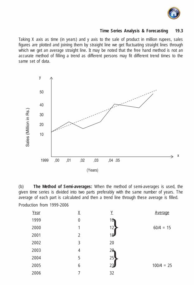
19.3Time Series Analysis & Forecasting
Taking X axis as time (in years) and y axis to the sale of product in million rupees, salesfigures are plotted and joining them by straight line we get fluctuating straight lines throughwhich we get an average straight line. It may be noted that the free hand method is not anaccurate method of filling a trend as different persons may fit different trend times to thesame set of data.
(b) The Method of Semi-averages: When the method of semi-averages is used, thegiven time series is divided into two parts preferably with the same number of years. Theaverage of each part is calculated and then a trend line through these average is filled.
Production from 1999-2006
Year X Y Average
1999 0 10
2000 1 12 60/4 = 15
2001 2 18
2002 3 20
2003 4 20
2004 5 25
2005 6 23 100/4 = 25
2006 7 32
}
}

19.4 Advanced Management Accounting
The average of first part of the data is 15 and that of the second part is 25. As 15 is theaverage of 1999, 2000, 2001 and 2002. 15 is plotted in between 2000 and 2001 which isthe middle of the 4 years period. Similarly 25 is plotted in between 204 and 2005. Thenthese points are joined by a straight line which is a semi-average trend line.
(c) The method of moving average: The method of moving averages is used not onlyto fit trend lines but also to seasonal and cyclical variation.
e.g. Find out the three year moving averages starting from 1989.
Year: 1989 1990 1991 1992 1993 1994 1995 1996 1997 1998 19992000
Sales: 10 15 20 25 15 12 15 24 15 21 15 24
(Rs. in million)
Solution: Taking the first three years 1989, 1990 and 1991, we add up their sales 10+15+20 = 45. This figure is written is column (3) against the mid year that is 1990. Nowdropping the year 1989 and including the year 1992 in the calculation and thus moving inthis manner the process is continued until we reach the last three years 1998, 1999 and2000. It may be noted that there are no moving total for the 1st and last year.

19.5Time Series Analysis & Forecasting
The next step involves the calculation of moving average by dividing the moving total by 3.
Table:
Year Sales 3 year moving 3 year moving
Rs. in Million total average
1989 10 — —
1990 15 45 15
1991 20 60 20
1992 25 60 20
1993 15 52 17
1994 12 42 14
1995 15 51 17
1996 24 54 18
1997 15 60 20
1998 21 54 18
1999 18 63 21
2000 24 — —
Effective Application of Moving Average Method:
To ensure result of moving average method to be appropriate and effective, it is required toascertain first whether a regular periodic cycle in the time series exists. In several casesone would find that there is a certain regularity in the series to allow the use of the movingaverage method. If may be also noted that if the basis nature of the time series is linear, itwill give a linear trend. In case of curvilinear nature, the trend will be curve. Moreovermoving average method helps to element seasonal fluctuation, for a time series.
Method of Least squares: Among the method of fitting straight line to a series of data, thismethod is the most frequently used method. The equation of a straight line is Y = a+ b´where X is the time period, say, year and Y is the value of the item measured against time,a is the Y- intercept and b is the coefficient of X indicating slope of the trend line.
In order to find a and b the following two equations are solved:
ΣY = ax + b Σx
ΣXY = a Σx + bΣx2
Where n is the total number of observations in a series. These equations are called normalequations.
e.g. Old number of years:
Year: 1996 1997 1998 1999 2000
Y 270 285 295 315 330

19.6 Advanced Management Accounting
Fit a linear trend to these data using method of least squares:
Solution:
Year x y xy x2
1996 -2 270 -540 4
1997 -1 285 -285 1
1998 0 295 0 0
1999 1 315 315 1
2000 2 330 -660 4
Total 0 =Σx 1,495 = Σy 150 =Σx y 10 = Σx2
Substituting these values in two normal equations.
We get
1495 = 5a +b (0) ………………..(1)
150 = a (0) +b (10) ……………..(2)
Equations (1) gives a = 1,495/5 = 299
Equations (2) gives b = 150/10 = 15
The straight line trend we get is
Y = 299 +15x (origin: year 1998)
(x = 1- year unit)
e.g. Even Number of years:
Year: 1985 1986 1987 1988 1989 1990
Y 15 14 18 20 17 24Fit a trend to these data using method of least squares.
Solution
Year x y xy x2
1985 -5 15 -75 25
1986 -3 14 -42 9
1987 -1 18 -18 1
1988 1 20 20 1
1989 3 17 51 9
1990 5 24 120 25
Total 0 =Σx 108 = Σy 56 =Σx y 70 = Σx 2

19.7Time Series Analysis & Forecasting
Two normal equations are:
ΣY = an +b Σx
ΣXY= aΣx +bΣx2
Substituting the values in the two equations, we get
108 = 6a +b (0) …………(1)
56 = a(0) +b (70)………(2)
Solving we get a = 108/6 = 18
And b = 56/70 = 0.8
The trend equation is Y = 18 +0.8 ´
Origin year: Mid of 1987-88
Unit of X = ½ year
Note:
(i) Putting values of x for different years we get values of y which are trend values (y)
(ii) For forecasting, to calculate the value of x, for a given future year and substituting thevalue of x in the trend equation to get the forecasted value.
Higher Degree Polynomial Trends:So far we have discussed linear trend which in fact is a polynomial trend of the first degree.However instead of straight line trend, some parabolic trend may be best fit when we haveto use second degree polynomial trend. This trend equation is
Y = a+bx+cx2
In this also method of least sequence is to be used where there are normal equationsΣ Y = na +b Σx + c Σx2
Σxy = a Σx +b Σx2 +c Σx3
Σx2y = aΣx2 +bΣx3 +c Σx4
e.g. fit quadratic trend:Year : 1995 1996 1997 1998 1999Production Of cars: 2 4 8 14 22(‘0000)
Solution
Year x x2 y xy x2y x3 x4
1995 -2 4 2 -4 8 -8 161996 -1 1 4 -4 4 -1 11997 0 0 8 0 0 0 01998 1 1 14 14 14 1 11999 2 4 22 44 88 8 16
Total 0 10 50 50 114 0 34

19.8 Advanced Management Accounting
Applying these values in the above equations, we get
50 = 5a +10c …………………..(1)
50 = 10b ……………………….(2)
114 = 10a +34c ……………….(3)
From (2) we find b = 50/10 = 5
Again, 50 = 5a + 10c ………………..(1)
114 = 10a + 34 c……………...(2)
(3) 114 = 10a + 34c
(1)×2 100 = 10a + 20c
14 = 14C
∴c = 1
From (1), 50 = 5a +10 ∴ a = 8
Required trend equation is
Y = a+ bx +cx2
Y = 8+5x +x2 origin year 1997
Unit of x = 1 year
Exercise
(1) Assuming an additive model, obtain 3 year-moving average to obtain the trend freeseries for year 1992 to 1996 from the following data:
Year: 1991 1992 1993 1994 1995 1996 1997
Export: 126 130 137 141 145 155 159
(Rs. in lakhs)
Answer: 131, 136, 141, 147, 153
(2) Use a 4 yearly moving average method to calculate trend for the following data:
Year: 1978 1979 1980 1981 1982 1983 1984 1985 1986 1987 1988
Production: 614 615 652 678 681 655 717 719 708 779 757
Answer: ___, ___, 648, 661.4, 674.63, 687.9, 690.1, 715.3, 735.8, ___, ____.
(3) Give below are the figures of production (in million tons) of wheat
Year: 1989 1990 1991 1992 1993 1994 1995
Production: 80 90 92 83 94 99 92
Fit a straight line trend to these figures.
Answer: Y = 90 +2x, origin year 1992, x unit = 1 year]

19.9Time Series Analysis & Forecasting
(4) Fit a straight line by the least squares method to the following figures of production ofSugar factory:
Year 1979 1980 1981 1982 1983 1984 1985
Production 76 87 95 81 91 96 90
Estimate the production for 1986.
Answer: Y=88+2x; 96 (‘000 tons)
(5) The following table given the annual profit (in thousand Rs.) in a factory
Year: 1991 1992 1993 1994 1995 1996 1997
Profit 60 72 75 65 80 85 90
Fit a straight line trend by the method of least squares. Also find annual trend of the profit.Also calculate the projected profit for 1998.
Answer: Y = 75.286 +4.321x, 4.321, 92.57 (‘000 Rs.)
(6) Below are given the annual consumption in thousand tons of a town
Year 1985 1986 1987 1988 1989 1990 1991
Consumption 70 75 90 91 95 98 100
(‘000 tons)
Fit a straight line trend by the method at least square and indicate the trend values by taking1988 as origin. Shift the origin to 1990 and find out the revised trend equation.
Construct the annual trend equation into monthly trend equation.
Answer. Y = 88.43 + 5.04x, Y = 98.51 +5.05x, Y = 7.37 +0.035 x]
(7) Fit a quadratic trend to the following data:
Year 1988 1989 1990 1991 1992
Value 180 192 195 204 202
Answer: Y = 197.74 +5.6x -1.57x2]
Detrending: The process of eliminating the trend is referred to as detrending and the trenditself can be represented either as a straight line or some type of smooth curve. What is leftafter elimination of trend is short term variation, expressed as:
S × C × I Under multiplicative model,
And S + C + I Under additive model.
19.3.2 The Calculation of Seasonal Variations
These are short-term movements which recur after a period. The period is normally lessthan a year-it may be a month or a quarter of the year. For example, the prices of grain varybetween the harvest season and the non-harvest season.

19.10 Advanced Management Accounting
For purpose of time series analysis we isolate the seasonal element. There are two majorreasons for this : (i) to study seasonal variation; and (ii) to eliminate them.
I. Seasonal Variations in themselves give a clear idea about the relative position ofeach season on the basis of which it is possible to plan for the season.
II. It is necessary to eliminate seasonal factor to get the cyclical or irregular factors.The is called deseasonalization of the data.
First we take an illustration of isolating short-term and seasonal fluctuations by the additivemodel.
Illustration:
Year Quarter Output Moving Moving Moving Short-term
Q Y total total Average Fluctuation
(4) (8) (T) Y-T=S+C+I
1971 1 35
2 86
312
3 67 627 78 -11
315
4 124 653 82 +42
338
1972 1 38 700 88 -50
362
2 109 776 97 +12
414
3 91 837 105 -14
423
4 176 895 112 +64
472

19.11Time Series Analysis & Forecasting
Year Quarter Output Moving Moving Moving Short-termQ Y total total Average Fluctuation
(4) (8) (T) Y-T=S+C+I1973 1 47 957 120 -73
4852 158 1020 128 +30
5353 104 1084 136 -32
5494 226 1117 140 +86
5681974 1 61 1166 146 -85
5982 177 1210 151 +26
6123 134 1235 154 -20
6234 240 1275 159 +81
6521975 1 72 1311 164 -92
6592 206 1385 173 +33
7263 1414 307
Calculations of seasonal fluctuations :
Year Q.1 Q.2 Q.3 Q.4
1971 -11 42
1972 -50 +12 -14 +64
1973 -73 +30 -32 +86
1974 -85 +26 -20 +81
1975 -92 +33
Total -300 +101 -77 +273
Average -75 +25 -19 +68

19.12 Advanced Management Accounting
Other Methods of finding short period variations
I. Simple Average : The method is very simple: average the data by months or quartersor years and them calculate the average for the period. Then find out, whatpercentage it is to the grand average.
Seasonal Index = Monthly or quarterly average
×100Grand Average of the months or the quarters
Same results are obtained if the totals of each month or each quarter are obtained insteadof the average of each month or each quarter.
Illustration
Year 1st Quarter 2nd Quarter 3rd Quarter 4th Quarter
1970 3.7 4.1 3.3 3.5
1971 3.7 3.9 3.6 3.5
1972 4.0 4.1 3.3 3.1
1973 3.3 4.4 4.0 4.1
Total 14.7 16.5 14.2 14.2
Quarterly 3.68 4.12 3.55 3.55
Average
Seasonal Index 98.7 110.8 95.3 95.3
The grand average = 3.68 4.12 3.55 3.55 14.90
3.724 4
+ + + = =
Seasonal Index = Quarterly Average
×100Grand Average
Seasonal Index for the quarters : 1st : 3.68
100 98.73.72
× =
2nd :4.12
100 110.83.72
× =
3rd and 4th3.55
100 95.33.72
× =
Example
Using the method of monthly averages determine the monthly indices for the following dataof production of a commodity for the year 1979,1980,1981.

19.13Time Series Analysis & Forecasting
Month 1979 1980 1981
Production in lacs of tons
January 12 15 16
February 11 14 15
March 10 13 14
April 14 16 16
May 15 16 15
June 15 15 17
July 16 17 16
August 13 12 13
September 11 13 10
October 10 12 10
November 12 13 11
December 15 14 15
Solution
Here, instead of dividing the monthly average by the overall average, we divide the monthlytotals by the average of totals.
Production in Lacks of tons
Year 1979 1980 1981 Seasonal Index
Month Totals (percentages)
January 12 15 16 43 104.9
February 11 14 15 40 97.5
March 10 13 14 37 90.2
April 14 16 16 46 112.2
May 15 16 15 46 112.2
June 15 15 17 47 114.6
July 16 17 16 49 119.5
August 13 12 13 38 92.6
September 11 13 10 34 82.9
October 10 12 10 32 78
November 12 13 11 36 87.8
December 15 14 15 44 107.3
Total 492
Average 41
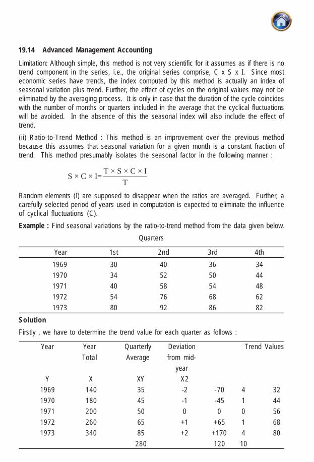
19.14 Advanced Management Accounting
Limitation: Although simple, this method is not very scientific for it assumes as if there is notrend component in the series, i.e., the original series comprise, C x S x I. Since mosteconomic series have trends, the index computed by this method is actually an index ofseasonal variation plus trend. Further, the effect of cycles on the original values may not beeliminated by the averaging process. It is only in case that the duration of the cycle coincideswith the number of months or quarters included in the average that the cyclical fluctuationswill be avoided. In the absence of this the seasonal index will also include the effect oftrend.
(ii) Ratio-to-Trend Method : This method is an improvement over the previous methodbecause this assumes that seasonal variation for a given month is a constant fraction oftrend. This method presumably isolates the seasonal factor in the following manner :
T × S × C × IS × C × I=
T
Random elements (I) are supposed to disappear when the ratios are averaged. Further, acarefully selected period of years used in computation is expected to eliminate the influenceof cyclical fluctuations (C).
Example : Find seasonal variations by the ratio-to-trend method from the data given below.
Quarters
Year 1st 2nd 3rd 4th
1969 30 40 36 34
1970 34 52 50 44
1971 40 58 54 48
1972 54 76 68 62
1973 80 92 86 82
Solution
Firstly , we have to determine the trend value for each quarter as follows :
Year Year Quarterly Deviation Trend Values
Total Average from mid-
year
Y X XY X2
1969 140 35 -2 -70 4 32
1970 180 45 -1 -45 1 44
1971 200 50 0 0 0 56
1972 260 65 +1 +65 1 68
1973 340 85 +2 +170 4 80
280 120 10

19.15Time Series Analysis & Forecasting
The value of the constants a and b in the equation of a straight line are as following :
Y 280a= = =56
N 5∑
, 2
XY 120a= = =12
X 10∑∑
The quarterly increment therefore is 12/4=3.
Since there are 4 quarters we have to take the point in between the 2nd and the 3rd quartereach year. Thus following are trend values for various quarters of the respective years.
Year 1st 2nd Yearly Trend 3rd 4th
Values
1969 27.5 30.5 32 33.5 36.5
1970 39.5 42.5 44 45.5 48.5
1971 51.5 54.5 56 54.5 60.5
1972 63.5 66.5 68 69.5 72.5
1973 75.5 78.5 80 81.5 84.5
Actual Quarterly Values As % of quarterly Trend Values :
1969 109.1 131.1 107.5 93.1
1970 86.1 122.4 109.9 90.7
1971 77.7 106.4 93.9 79.3
1972 85.0 114.3 97.8 85.5
1973 106.0 117.1 105.5 97.0
Total 463.9 591.3 514.6 445.6
Average 92.78 118.26 102.92 89.12
Seasonal Index
Adjusted 92.0 117.4 102.1 88.4
Since the total of the seasonal index is 403.08 = (92.88+118.26+102.92+89.12).
Each index has to be adjusted by multiplying it by 400
403.08 and the final indices are thus
available.
(iii) Ratio-to-Moving Average Method : In this method instead of calculating the annualtrend by the method of least squares the moving average is used. It is more suitable whenseasonal variations for the months are to be calculated:

19.16 Advanced Management Accounting
Link Relative Method
(i) To Calculate Seasonal Link Relative for each season where
Link Relative = Current Season Figure
×100Previous Season Figure
(ii) Calculate average of the link relatives for each season. Arithmetic mean is generallyused but even median could be used.
(iii) Convert there averages into chain relatives on the basis of first season.
(iv) Calculate the Chain relative of the first season on the basis of the last season.
(v) For correction, the chain relative of the first season calculated by the first method isdeducted from the chain relative of the first season calculated by the second method.The difference is divided by the number of seasons. The resulting figure multiplied by1,2,3, etc. are deducted respectively from the chain relatives of 2nd,3rd ,4th, etc. seasons.
(vi) The seasonal indices are available when we express the corrected chain relatives aspercentages of their respective averages.
Example : Apply the method of link relatives to the following data and calculate seasonalindices.
Quarter 1969 1970 1971 1972 1973
I 4.5 4.8 4.9 5.2 6.0
II 5.4 5.6 6.3 6.5 7.0
III 7.2 6.3 7.0 7.5 8.4
IV 6.0 5.6 6.5 7.2 6.7
Solution : Let us first calculate link relatives of the seasonal figures.
These are given below in the table:
Quarters
Year I II III IV
1969 120 133 83
1970 80 117 113 89
1971 88 129 111 93
1972 80 125 115 96
1973 83 117 120 80
Mean 82.8 121.6 118.4 88

19.17Time Series Analysis & Forecasting
Chain Relatives 100100 121.6
100
×
121.6 118.4
100
× 143.9 88
100
×
= 121.6 = 143.9 = 126.6
Corrected chain100 121.6-1.2 143.9-2.4 126.6-3.6
= 120.4 = 141.5 = 123
Seasonal Indices100 100
121.2
× 120.4 100
121.2
× 141.5 100
121.2
× 123.0 100
121.2
×
= 82.5 = 99.4 = 116.7 = 101.5
Note : The link relatives are calculated by dividing the value of one quarter by the value ofthe previous quarter and expressing them as percentages.
For example, Link Relative of 1969-Quarter II =5.4
1004.5
×
= 120
Link Relative of 1969-Quarter III =7.2
1005.4
×
= 133
The figure correction has been calculated as follows :
Chain relative of the first quarter on the basis of first quarter = 100
Chain relative of first quarter on the basis on the last quarter = 82.8 126.6
104.8100
× =
The difference between these chain relatives = 104.8 – 100 = 4.8
Difference per quarter 4.8
124
=
Seasonal variation indices have been calculated as follows
Average corrected chain relatives = 100 120.4 141.5 123.0
121.24
+ + + =
Seasonal variation indices therefore will be calculated as :
Corrected chain relative=100
121.2

19.18 Advanced Management Accounting
Deseasonalization : The process of eliminating seasonal fluctuations or deseasonalizationof data consists of dividing each value in the original series by the corresponding value ofthe seasonal index. The following table will illustrate this.
Quarter Original Value Seasonal Index Deseasonal Value
I 272 79.000 344
II 381 120.153 317
III 346 109.583 315
IV 279 91.264 305
19.4 SMOOTHING METHODS IN TIME SERIES
Exponential Smoothing
The methods of analyzing the time series discussed earlier are usually employed for longterm forecasting. But there are numerous situations e.g. , warehouse, consumer stores andmanufacturing organizations which need future forecasts just over the next month, week oreven a day, for each of the item individually.
It is not uncommon to find thousands and even lakhs of items in such organizations and,therefore, as many forecasts may have to be raised to maintain sufficient stocks of items.Excess stocking would adversely affect the service to the customer or hold up assembly ofthe final product.
Moving Averages method could indeed be applied in such situations, but it would requirekeeping in the records of the past sales figures as many in number as the moving averageperiod. This would require too much clerical recording or in a computerized system,storage space in the computer files.
Exponential smoothing is a quicker and theoretically more sound method of short-termforecasting. Its major, though not exclusive, use, however, is in Production and Inventorycontrol.
Exponential Smoothing as an Average
Consider the Moving Average (Period = 4 months) for the following series :
20 24 28 30
Moving Average = 1
(20 24 28 30)4
× + + +
= 1 1 1 1
20 24 28 304 4 4 4
× + × + × + ×
= 1 2 3 1W ×20+W ×24+W ×28+W ×30

19.19Time Series Analysis & Forecasting
It may be noted that the weight ages W1, W2, W3 and W4 assigned to each observation
is equal and 1
4 of that is reciprocal of the Moving Average period. Since the sum of the
weight is unity the Moving Average is a true average.
Exponential Smoothing is also an average in this sense. But the weight ages assigned tothe past figures are not equal. The most recent observation is assigned the highest weightage and it decreases in geometric as we move towards the older observations. This isobviously more reasonable because the most recent observation is more relevant forforecasting the future sales than an older observation. The ratio of the geometric
progression of the series of the weights is (1-�� , where α is a constant called smoothingcoefficient. Theoretically all the past observations are needed for computing the exponentiallysmoothed average, that is the sequence of the past sales figures may run indefinitely toinfinity. Despite this, as will be noted below, the method is remarkably easy to apply inpractice.
The discussion should be more clear from the following table:
(The sum of the column C gives the exponentially smoothed average, ut)
Observations at time t Weightage Assigned Col.(A) x Col (B)
(A) (B) (C)
ty α tyα
1ty − (1 )α α− 1(1 ) tyα α −−
2ty −2(1 )α α− 2 2(1 ) tyα α −−
3ty −3(1 )α α− 3
3(1 ) tyα α −−
t ny − (1 )nα α− (1 )nt nyα α −−
Exp. Sm. Average. 21 1 2(1 ) (1 ) .... (1 ) ...n
t t t t nu y y y yα α α α α α α− − −= + − + − + − +
This average may be used as the forecast for the next period , a in theory may be between0 to 1: but in practice between 0.1 to 0.3.
It is to be contrasted with the moving average method in that infinite number of the pastfigures are being utilized, here. This looks awesome but a great deal of simplification ispossible.
From Col. B i t is obvious that the weights are decreasing exponential ly2[ , (1 ), (1 ) ,...]α α α α α− − . Hence the name exponential smoothing.

19.20 Advanced Management Accounting
An essential feature of a true moving average is that the sum of the weights should be unity.Let us ascertain this for Exponential smoothing by summing up the column B.
2
(1 ) .... (1 ) ...
{1 (1 ) 1 ) ...}
1 (1 )1 (1 )
1 (1 )
n
nn
α α α α αα α α
αα αα
+ − + − +− − + − +
⎡ ⎤− −= = − −⎢ ⎥− −⎣ ⎦
As n approaches , (1 )α∞ − being less than 1, approaches 0. Therefore, the sum of theweights is unity.
Procedure for Computations
1 1 1(1 ) ..... (1 ) .....nt t ny y yμ α α α α α− −= + − + − +
1 1 1 2(1 ){ (1 ) .....}t ty y yμ α α α α α− −= + − + − +
1 1 1(1 ) tyμ α α μ −= + −
1 1 1 1( )t t tyμ μ α μ− − −= + −
The term in the bracket on R.H.S> is the differences between latest observation and itsforecast raised a period earlier. It is therefore, the error, and is denoted by e1
1 1t teμ μ α−= +
The procedure for computations is summarized below:
(i) Find the error by subtracting the recent average from the incoming observation.
(ii) Multiply error e1 by a. This is the correction to be applied to the past average.
(iii) Add the correction to the past coverage 1 1tμ μ −= . This gives new average u1 as the
forecast for the next period. The rationale behind this is further clarified in the followingfigure:

19.21Time Series Analysis & Forecasting
The figure gives the forecasts prior to the period t. 1tμ − is the forecast for the period t
raised at period (t-1). The actual sales that materializes between the period t-1 and t areaverage y
t. The sales have exceeded the forecast. In view of this we should tend to modify
the average :e is the error. The modification is done by increasing the average by e,.Thus the difference between each new incoming observation and its forecast is beingutilized in keeping the average up-to-date.
Value of the Smoothing Co-efficient
Consider the two extremes α = 0 and α = 1
(i) α=0
(ii) The correction to be applied to the forecast is α=0. This implies that the earlieraverage stands and no account of any difference between actual observation andits forecast is taken α=0, therefore , implies that the forecasting system does notreact to the incoming observations.
(iii) μ1 = μτ−1 + e1 = μτ−1 + (yt – μτ−1) = y1
Here the observation itself is taken as the forecast for the next period. The pastseries is completely ignored.
This should suggest that a low value of gives more weightage to the past figures andless consideration to the incoming observation. Low values are therefore, to be used wherethe series is stable and high values where the series is rather fluctuating.
Eg:1. The actual figures for the sales of bleaching, powder for the year 1973 are shownbelow in Column A in the table below. The forecasts or the estimates using Exponentialsmoothing are required , α =0.3. Initial forecast may be taken as 29.6.

19.22 Advanced Management Accounting
Month Sales Error Correction Forecast
(A) (B) = (A) - (D) (C) = (B) x 0.3 (D)
Jan. 33 33-29.6=3.4 3.4 x 0.3 = 1.0 29.6 (Initial)
Feb 31 31.30.6=04 0.4 x 0.3 = 0.1 29.6+1 = 30.6
Mar 34 34-30.7=3.3 1 30.6+0.1=30.7
Apr 32 32-31.7=0.3 0.1 30.7+1=31.7
May 37 37-31.8=5.2 1.6 31.8
Jun 36 36-33.4=2.6 0.8 33.4
Jul 34 34-34.2=-0.2 -0.1 34.2
Aug 32 32-34.1=-2.1 -0.6 34.1
Sep 41 41-33.5=7.5 2.2 33.5
Oct 44 44.35.7=8.3 2.5 35.7
Nov 44 44.38.2=5.8 1.7 38.2
Dec 50 50-39.9=10.1 3.0 39.9
Note: (i) Each fig in col (d) is obtained by adding to its earlier figure the correction incolumn (c).
(ii) Initial estimate of 29.6 was given. When exponential smoothing is introduced thisestimate would invariably be needed to start the system. It may be subjectively guessedor simple arithmetic mean of the past figures may be taken.
To summarise the discussion on Exponential smoothing thus far:
(A) Exponential smoothing, as against its contender the Moving Averages Method, isappealing because of the better weight age scheme.
(B) The greatest disadvantage inherent in the Moving Averages is relatively large amountof historical data that must be retained to compute them. The longer, the averaging period,the more the data that must be retained. In Exponential smoothing, records need tobe kept just for α and the latest average.
(C) Basically, Exponential smoothing provides a convenient, systematic method for revisingthe forecast for the next period whenever discrepancy exists between the previous forecastsales for the current period and the actual demand for the current period. If actual demandin the current period is higher than the forecast demand for the current period, the forecastfor the next period should be adjusted upwards. The amount of adjustment is determinedby the selected smoothing coefficient, the greater the constant the greater the adjustmentand vice versa. In fact, if the behavior of the sales series changes say, from a stable one toa fluctuating one, may be changed to be responsive to the new behavior.

19.23Time Series Analysis & Forecasting
19.5 EXISTENCE OF TREND
The students might note in the solved example above by comparing column A with D thatthe forecast tends to be lower than the actual sales. This is because there exists a trend inthe sales figures. The sales which is around 30 at commencement of the year 1973 haverisen to 50 at the end.
The diagram below brings out the behaviour of the Exponentially smoothed average withregard to series depicting trend.
Thus the Exponential smoothed average lags the sales series with trend. The followingequations [proof having been omitted] may be used, where trend is expected:
tu gives the necessary forecast for the next period at time period t.

19.24 Advanced Management Accounting
Example 2 : Exponential Smoothing for series with Trend.
Assumed : Initial Trend = -3.00, Initial Average = 750.00, 0.1α =
Period Sales Smoothed Smoothed Forecast Forecast
Average Trend Error
0 750 -3.00
1 720 747 -3.00
2 670 739.3 -3.47 717.0 47.00
3 680 733.37 -3.72 704.6 24.60
4 740 734.03 -3.28 696.2 -43.79
5 720 732.63 -3.09 701.3 -18.75
6 940 753.37 -0.71 701.7 -238.28
7 1020 780.03 2.03 746.3 -273.71
8 1220 824.03 6.23 800.3 -419.63
9 1260 867.62 9.96 886.3 -373.71
10 1300 910.86 13.29 967.3 -332.74
11 1190 938.78 14.75 1043.8 -146.2312 1080 952.90 14.69 1086.3 6.30
Consider Period 1.
1 1 1
1 1 0
1 1
( ) 750 0.1(750 750) 747
( ) (1 ) 0.1( 3.00) 0.9( 3.00) 3.00
11 747 10( 3.00) 717
o o
o
t
u u e y u
u u
u u
α αλ α α λ
α λα
= + = − = + − == − + − = − + − = −
−⎛ ⎞= + + = + − =⎜ ⎟⎝ ⎠
Forecast Error = 717-670 = 47. (Entered in the last column)
Consider Period 2
2 1 1 1 2 1
2 2 1 1
2 2 2
( ) 747 0.1(670 747) 739.30
( ) (1 ) 0.1(739.30 747) 0.9( 3.00) 3.47
10 739.30 34.70 704.60
u u e u y u
u u
u u
α αλ α α λ
λ
= + = + − = + − == − + − = − + − = −= + = − =
Forecast Error. = 704.6 – 680 = 24.6
It is to be noted that the trend factor , 1λ is also recursively exponentially smoothed for every
period.

19.25Time Series Analysis & Forecasting
The student may carry on with the rest of calculation for practice by verifying with thefigures in the table.
Optimum Value of the Smoothing Coefficient
In the above example, the forecast errors are given in the last column. These, whensquared and accumulated, give a measure of the discrepancy between the forecasts and
the actual sales. Similarly, other values of 0.2,0.3,α = etc. may be tried. The value thatgives the least squared diviation of error would be optimum α . In practice, it is not infrequentto assign the value of a from experience. Where the computer activities are available, theabove method of least squared deviations may be carried out for groups of items depictingsimilar sales behaviour.
Limitation of Exponential Smoothing
(i) The method is useful for short-term forecasting only.
(ii) It relies solely on the past history of sales. There are cases where subjectiveestimates may provide better forecasts. There have been attempt to complement thetwo; forecasts from Exponential smoothing and subjective estimates, successful to agreat extent, but not fully satisfactory.
Further Extension
The method of Exponential smoothing is quite versatile and: trend can be extended toaccount for seasonal variations. Just as the initial, forecast and trend factors are estimatedand then recursively adjusted in the light of the discrepancy between the forecast and theincoming observation; seasonal factors can be similarly initially estimated, incorporated inthe model and then recursively adjusted. For short-term forecasting, it has almost universallysuperseded the Moving Average method. The method is particularly favoured withcomputerized applications because of the minimal data items that need to be stored.
19.6 FORECASTING USING TIME SERIES
Since economic and business conditions very over time, business leaders must find waysto keep in touch with the effects that such change will have on their particular operations.One technique which business managers may use as an aid in planning for future needs isforecasting. There are basically two types of forecasting called qualitative and quantitative.Qualitative forecasting methods are useful when historical data are unavailable. Quantitativemethods make use of historical data for forecasting. Quantitative forecasting methods canbe subdivided into two types, namely, time series and causal. Causal forecasting methodsinvolved the determination of factors which relate to the variable to be predicted. On theother hand, time series forecasting methods involve the projection of future values of avariable based entirely on the past and present observation of that variable. In this sectionwe will see the various forecasting methods using time series.
(i) Mean Forecast : The simplest forecasting method in which for the time period t. weforecast the value of the series to be equal to the mean of the series;
ty y=

19.26 Advanced Management Accounting
This method is not adequate as trend effects and the cyclical effects are not takeninto account in this.
(ii) Naïve forecast : In this method, by taking advantage of the fact that there may be highcorrelation between successive pairs of values in a time series, we forecast the value,for the time period t, to-be equal to the actual value observed in the previous period tthat is, time period (t – 1):
1t ty y −=
(iii) Linear Trend Forecast : In this method , a linear relationship between the time andthe response value has been found from the linear relationship.
ty a bX= +
where X will be found from the value of t and a and b are constants.
(iv) Non-linear Trend Forecast : In this method, a non-linear relationship between thetime and the response value has been found again by least-squares method. Thenthe value, for the time period t , will be calculated from the non-linear equation . i.e.,
2ty a bX cX= + +
where X-value will be calculated from the value of t.
(v) Forecasting will Exponential Smoothing : In this method, the forecast value for thetime period t is found using exponential smoothing of time series. Specifically, at thetime period t.
1 1( )t t t ty y y yα− −= + −
where the forecasted value for time period t + 1 ;
yt-1
= the forecasted value for time period t. :
yt=the observed value for time period t.
We will see the usefulness of these formulae with an example.
Example : The following time series data are given. Find the forecast for various yearsusing mean forecast, naïve forecast, linear trend forecast, non-linear trend forecast.
Year 1980 1981 1982 1983 1984 1985
Sales (Rs. In Crores) 24.5 25.9 27.6 30.1 34.8 41.5
Solution
We list the various forecasting values in a table:
From the table, one can easily see that the observed and the forecast values using quadratictrend setting method do not differ much. Hence, here forecasting for future years can bedone using quadratic trend setting. For example the forecast for 1991 will be Rs.48.69crores. This is found from the quadratic equation 24.87 – 0.17 X + 0.69 X2 with base year

19.27Time Series Analysis & Forecasting
as 1985 i.e. X= t – 1985.
Table 2 : Comparison of from forecasting methods.
Year Observed Forecast value
value Mean Naïve Linear Quadratic
y1 yt=y=30.73 yt=yt-1 yt=22.58 + yt = 24.87-
3.26 X 0.17X + 0.69X2
1985 24.5 30.73 22.58 24.87
1986 25.9 30.73 24.5 25.84 25.38
1987 27.6 30.73 25.9 29.1 24.27
1988 30.1 30.73 27.6 32.36 30.53
1989 34.8 30.73 30.1 35.63 35.17
1990 41.5 30.73 34.8 38.89 41.19
SUMMARY
� Utilities of time series analysis� Helps in evaluating current accomplishments� Helps in planning future operations� Facilitates comparisons� Helps in understanding past behaviour
� Components of time series� Secular trend (T)� Seasonal variations (S)� Cyclical variations (C)� Irregular variations (I)
� Methods for determining trend� Freehand� Semi average� Moving average� Least squares
� Methods for computing an index of seasonal variations� Simple average� Ratio to trends� Ratio to moving average� Link relative

19.28 Advanced Management Accounting
SELF-EXAMINATOIN QUESTIONS
1. Calculate the seasonal indices in the case of the following quarterly data in certainunits assuming no trend in the data:
Year Quarter
I II III IV
1980 39 21 52 81
1981 45 23 63 76
1982 44 26 69 75
1983 53 26 64 84
Answer: 86.4, 44.4, 118.4 , 150.8)
2. The number of production in Bombay in from Quarters of a year during the period1997- 1997 are given below:
Year Quarter
I II III IV
1987 165 135 140 180
1988 152 121 127 163
1989 44 26 69 75
Find the seasonal indices by Trend ratio method assuming a linear trend for thedata.
Answer: 105, 83, 89, 123)
3. Compute Seasonal indices from the following data using method of Link Relatives.
Year Quarter
I II III IV
1978 65 58 56 61
1979 68 63 63 67
1980 70 59 56 52
1981 60 55 51 58
Answer: 109,98,94,99)
An old forecast of 39 is given initially and the smoothing co-efficient is 0.1. Smoothexponentially the following observations: 41,41,34,39,36,35,40,36,41,33.
Answer: 39.2, 39.38, 38.84, 38.86, 38.57, 38.21, 38.39, 38, 15, 38, 43, 37, 89)