Advanced LWIR hyperspectral sensor for on-the-move proximal

detection of liquid/solid contaminants on surfaces Jay P. Giblin

*, John Dixon, Julia R. Dupuis, Bogdan R. Cosofret, William J. Marinelli

Physical Sciences Inc., 20 New England Business Center, Andover, MA, USA 01810

ABSTRACT

Sensor technologies capable of detecting low vapor pressure liquid surface contaminants, as well as solids, in a non-

contact fashion while on-the-move continues to be an important need for the U.S. Army. In this paper, we discuss the

development of a long-wave infrared (LWIR, 8-10.5 µm) spatial heterodyne spectrometer coupled with an LWIR

illuminator and an automated detection algorithm for detection of surface contaminants from a moving vehicle. The

system is designed to detect surface contaminants by repetitively collecting LWIR reflectance spectra of the ground.

Detection and identification of surface contaminants is based on spectral correlation of the measured LWIR ground

reflectance spectra with high fidelity library spectra and the system’s cumulative binary detection response from the

sampled ground. We present the concepts of the detection algorithm through a discussion of the system signal model. In

addition, we present reflectance spectra of surfaces contaminated with a liquid CWA simulant, triethyl phosphate (TEP),

and a solid simulant, acetaminophen acquired while the sensor was stationary and on-the-move. Surfaces included

CARC painted steel, asphalt, concrete, and sand. The data collected was analyzed to determine the probability of

detecting 800 µm diameter contaminant particles at a 0.5 g/m2 areal density with the SHSCAD traversing a surface.

Keywords: spatial heterodyne spectrometer, long wave infrared, chemical warfare agents, on-the-move detection,

non-contact detection, reflectance spectroscopy

1. INTRODUCTION

This paper describes the development of a non-contact sensing capability for on-the-move detection of surface

contaminants. The capability is based on a Long Wave Infrared (LWIR) spatial heterodyne spectrometer (SHS) coupled

with an LWIR illuminator. The sensor, referred to as the Spatial Heterodyne Surface Chemical Agent Detector

(SHSCAD) is designed to detect surface contaminants by repetitively collecting reflectance spectra of the ground when

employed on a moving vehicle. The system implements an SHS because it possesses an étendue that is an order of

magnitude larger than a conventional slit spectrometer. Consequently, even at the inherently short dwell times associated

with on-the-move sensing, the sensor’s noise equivalent spectral radiance (NESR) is sufficiently to support the detection

of liquid droplets or solid particles at surface densities of 0.5 g/m2. Additionally, an SHS acquires all of the spectral

bands of the ground within its field-of-view simultaneously (‘snapshot’ spectral acquisition), which is an essential

capability for on-the-move detection. Finally, the acquisition of the spectral signature occurs without the need for

moving optical components, thus providing a path to a ruggedized system for field operation.

Developmental efforts to have implemented an LWIR illuminator consisting of a high temperature globar and a COTS

elliptical reflector. The globar is imaged onto a target surface and modulated with a custom cylindrical chopper.

Modulation of the LWIR illuminator enables thermal background radiance removal from target surface and eliminates

clutter noise introduced by changing surface temperatures. The detection approach is based on collecting interferogram

data at the SHS sensor to form a time series of spectra. Each spectrum in the series corresponds to a different location on

the ground along the vehicle’s path of travel. Spectra from the time series are continuously processed by a detection

algorithm resulting in a series of single pixel detection decisions. The system’s overall detection decision is made based

on the cumulative response (i.e. total number of detection decisions) observed within a block of time. A contamination

alert is issued if the cumulative response over a desired length scale exceeds a predetermined threshold associated with

the desired constant false alarm rate.

Within this paper, we discuss the detection phenomenology of surface contaminants with the system. Derived system

requirements are presented based on a model of expected SHCAD output surface reflectance spectra. We introduce the

* jgiblin@psicorp.com; phone 1 978 689-0003; fax 1 978 689-3232; psicorp.com

optical and mechanical design of the SHSCAD. In addition, we present reflectance spectra of surfaces contaminated with

a liquid CWA simulant, triethyl phosphate (TEP) and the solid simulant acetaminophen, acquired with the sensor in both

stationary and on on-the-move configurations. Contaminated surfaces included CARC painted steel, asphalt, concrete,

and sand. The data collected was analyzed to determine the probability of detecting 800 µm diameter contaminant

particles at a 0.5 g/m2 areal density with the SHSCAD traversing a surface.

2. DETECTION APPROACH

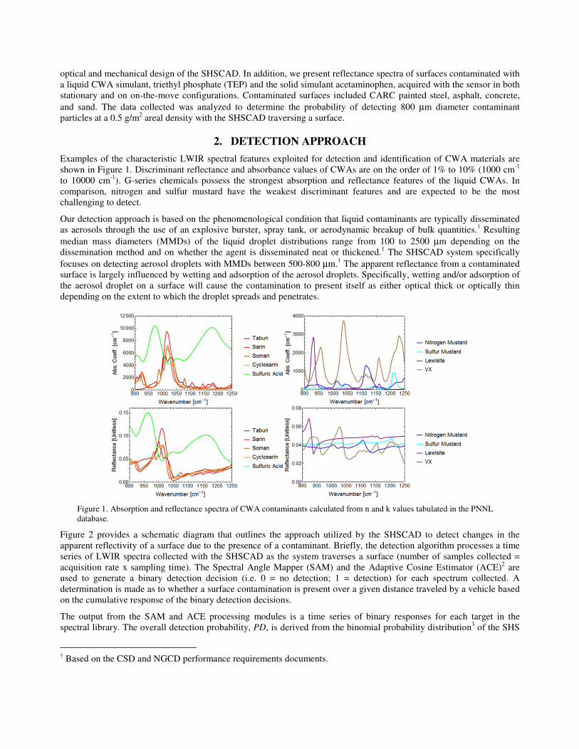
Examples of the characteristic LWIR spectral features exploited for detection and identification of CWA materials are

shown in Figure 1. Discriminant reflectance and absorbance values of CWAs are on the order of 1% to 10% (1000 cm-1

to 10000 cm-1

). G-series chemicals possess the strongest absorption and reflectance features of the liquid CWAs. In

comparison, nitrogen and sulfur mustard have the weakest discriminant features and are expected to be the most

challenging to detect.

Our detection approach is based on the phenomenological condition that liquid contaminants are typically disseminated

as aerosols through the use of an explosive burster, spray tank, or aerodynamic breakup of bulk quantities.1 Resulting

median mass diameters (MMDs) of the liquid droplet distributions range from 100 to 2500 µm depending on the

dissemination method and on whether the agent is disseminated neat or thickened.1 The SHSCAD system specifically

focuses on detecting aerosol droplets with MMDs between 500-800 µm.† The apparent reflectance from a contaminated

surface is largely influenced by wetting and adsorption of the aerosol droplets. Specifically, wetting and/or adsorption of

the aerosol droplet on a surface will cause the contamination to present itself as either optical thick or optically thin

depending on the extent to which the droplet spreads and penetrates.

Figure 1. Absorption and reflectance spectra of CWA contaminants calculated from n and k values tabulated in the PNNL

database.

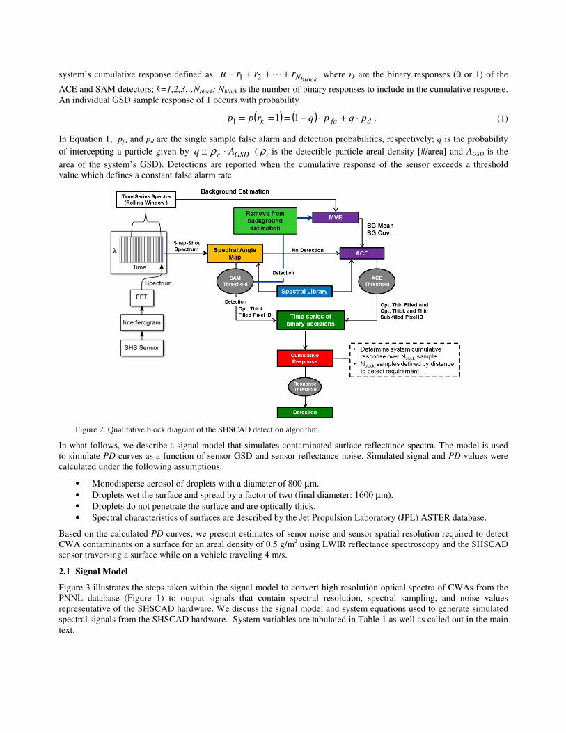
Figure 2 provides a schematic diagram that outlines the approach utilized by the SHSCAD to detect changes in the

apparent reflectivity of a surface due to the presence of a contaminant. Briefly, the detection algorithm processes a time

series of LWIR spectra collected with the SHSCAD as the system traverses a surface (number of samples collected =

acquisition rate x sampling time). The Spectral Angle Mapper (SAM) and the Adaptive Cosine Estimator (ACE)2 are

used to generate a binary detection decision (i.e. 0 = no detection; 1 = detection) for each spectrum collected. A

determination is made as to whether a surface contamination is present over a given distance traveled by a vehicle based

on the cumulative response of the binary detection decisions.

The output from the SAM and ACE processing modules is a time series of binary responses for each target in the

spectral library. The overall detection probability, PD, is derived from the binomial probability distribution3 of the SHS

† Based on the CSD and NGCD performance requirements documents.

system’s cumulative response defined as blockNrrru +++− L21 where rk are the binary responses (0 or 1) of the

ACE and SAM detectors; k=1,2,3…Nblock; Nblock is the number of binary responses to include in the cumulative response.

An individual GSD sample response of 1 occurs with probability

( ) ( ) dfak pqpqrpp ⋅+⋅−=== 111 . (1)

In Equation 1, pfa and pd are the single sample false alarm and detection probabilities, respectively; q is the probability

of intercepting a particle given by GSDc Aq ⋅≅ ρ ( cρ is the detectible particle areal density [#/area] and AGSD is the

area of the system’s GSD). Detections are reported when the cumulative response of the sensor exceeds a threshold

value which defines a constant false alarm rate.

Figure 2. Qualitative block diagram of the SHSCAD detection algorithm.

In what follows, we describe a signal model that simulates contaminated surface reflectance spectra. The model is used

to simulate PD curves as a function of sensor GSD and sensor reflectance noise. Simulated signal and PD values were

calculated under the following assumptions:

• Monodisperse aerosol of droplets with a diameter of 800 µm.

• Droplets wet the surface and spread by a factor of two (final diameter: 1600 µm).

• Droplets do not penetrate the surface and are optically thick.

• Spectral characteristics of surfaces are described by the Jet Propulsion Laboratory (JPL) ASTER database.

Based on the calculated PD curves, we present estimates of senor noise and sensor spatial resolution required to detect

CWA contaminants on a surface for an areal density of 0.5 g/m2 using LWIR reflectance spectroscopy and the SHSCAD

sensor traversing a surface while on a vehicle traveling 4 m/s.

2.1 Signal Model

Figure 3 illustrates the steps taken within the signal model to convert high resolution optical spectra of CWAs from the

PNNL database (Figure 1) to output signals that contain spectral resolution, spectral sampling, and noise values

representative of the SHSCAD hardware. We discuss the signal model and system equations used to generate simulated

spectral signals from the SHSCAD hardware. System variables are tabulated in Table 1 as well as called out in the main

text.

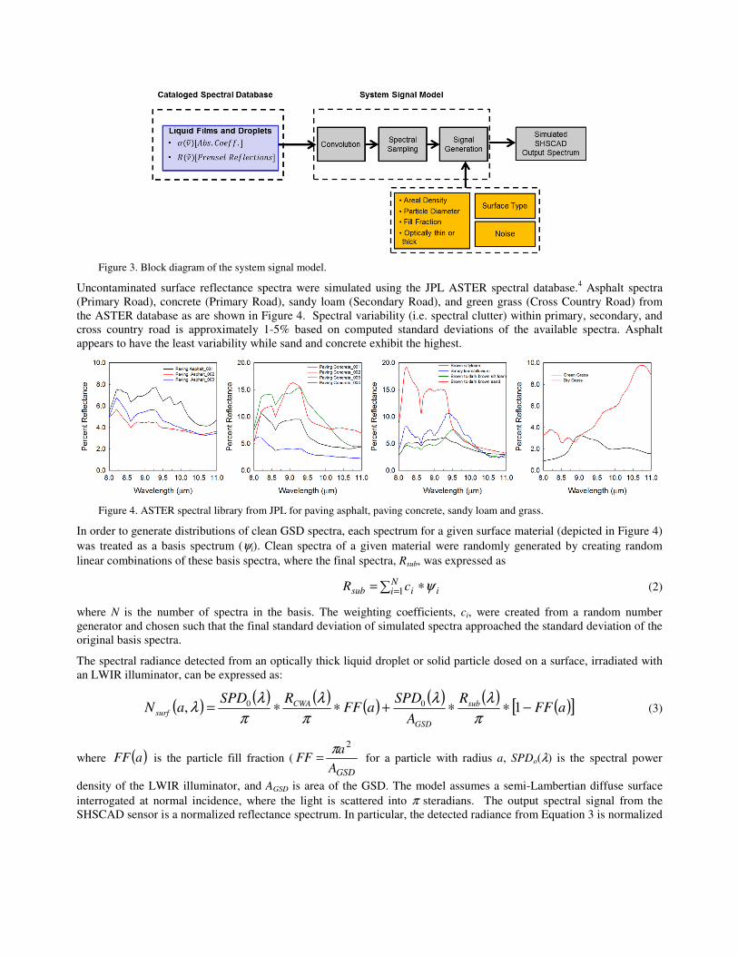
Figure 3. Block diagram of the system signal model.

Uncontaminated surface reflectance spectra were simulated using the JPL ASTER spectral database.4 Asphalt spectra

(Primary Road), concrete (Primary Road), sandy loam (Secondary Road), and green grass (Cross Country Road) from

the ASTER database as are shown in Figure 4. Spectral variability (i.e. spectral clutter) within primary, secondary, and

cross country road is approximately 1-5% based on computed standard deviations of the available spectra. Asphalt

appears to have the least variability while sand and concrete exhibit the highest.

Figure 4. ASTER spectral library from JPL for paving asphalt, paving concrete, sandy loam and grass.

In order to generate distributions of clean GSD spectra, each spectrum for a given surface material (depicted in Figure 4)

was treated as a basis spectrum (ψi). Clean spectra of a given material were randomly generated by creating random

linear combinations of these basis spectra, where the final spectra, Rsub, was expressed as

∑ = ∗= Ni iisub cR 1 ψ (2)

where N is the number of spectra in the basis. The weighting coefficients, ci, were created from a random number

generator and chosen such that the final standard deviation of simulated spectra approached the standard deviation of the

original basis spectra.

The spectral radiance detected from an optically thick liquid droplet or solid particle dosed on a surface, irradiated with

an LWIR illuminator, can be expressed as:

( ) ( ) ( ) ( ) ( ) ( ) ( )[ ]aFFR

A

SPDaFF

RSPDaN sub

GSD

CWAsurf −∗∗+∗∗= 1, 00

π

λλ

π

λ

π

λλ (3)

where ( )aFF is the particle fill fraction (

GSDA

aFF

2π= for a particle with radius a, SPDo(λ) is the spectral power

density of the LWIR illuminator, and AGSD is area of the GSD. The model assumes a semi-Lambertian diffuse surface

interrogated at normal incidence, where the light is scattered into π steradians. The output spectral signal from the

SHSCAD sensor is a normalized reflectance spectrum. In particular, the detected radiance from Equation 3 is normalized

by the radiance detected from an Infragold substrate irradiated with the LWIR illuminator. The detected Infragold

radiance is written as

( )( ) ( )

π

λλλ IG

GSDIG

R

A

SPDN ∗= 0

(4)

The apparent reflection from the contaminated surface can be expressed as

( )( )

( )( ) ( ) ( ) ( )[ ]aFFRaFFR

N

NR SubCWA

IG

Surf

Surf −∗+∗== 1λλλ

λλ (5)

where RIG (λ)= 1. The final simulated signal output of the SHSCAD, including Gaussian noise (��) is given by:

( ) ( ) ( ) ( ) ( )[ ] RaFFRaFFRR SubCWASurf δλλλ +−∗+∗= 1 (6)

Table 1. Key Variables used to Model the SHSCAD Spectral Signal for Liquid Droplets and Solid Particles

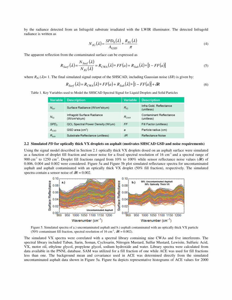
2.2 Simulated PD for optically thick VX droplets on asphalt (motivates SHSCAD GSD and noise requirements)

Using the signal model described in Section 2.1 optically thick VX droplets dosed on an asphalt surface were simulated

as a function of droplet fill fraction and sensor noise for a fixed spectral resolution of 16 cm-1

and a spectral range of

900 cm-1

to 1250 cm-1

. Droplet fill fractions ranged from 10% to 100% while sensor reflectance noise values (δR) of

0.006, 0.004 and 0.002 were considered. Figure 5a and Figure 5b plot simulated reflectance spectra for uncontaminated

asphalt and asphalt contaminated with an optically thick VX droplet (50% fill fraction), respectively. The simulated

spectra contain a sensor noise of δR = 0.002.

Figure 5. Simulated spectra of a.) uncontaminated asphalt and b.) asphalt contaminated with an optically thick VX particle

(50% contaminant fill fraction, spectral resolution of 16 cm-1, δR = 0.002).

The simulated VX spectra were correlated with a spectral library containing nine CWAs and five interferents. The

spectral library included Tabun, Sarin, Soman, Cyclosarin, Nitrogen Mustard, Sulfur Mustard, Lewisite, Sulfuric Acid,

VX, motor oil, ethylene glycol, propylene glycol, sodium hydroxide and water. Library spectra were calculated from

data available in the PNNL database. SAM was utilized for a fill fraction of one while ACE was used for fill fractions

less than one. The background mean and covariance used in ACE was determined directly from the simulated

uncontaminated asphalt data shown in Figure 5a. Figure 6a depicts representative histograms of ACE values for 2000

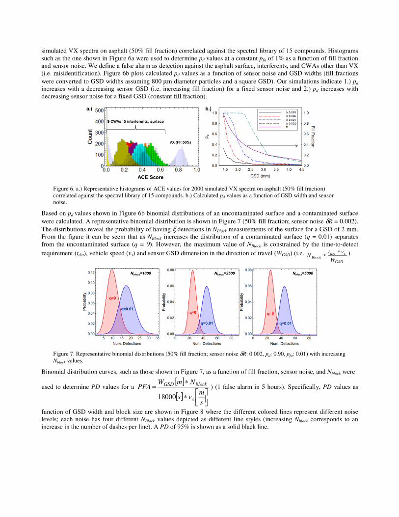
simulated VX spectra on asphalt (50% fill fraction) correlated against the spectral library of 15 compounds. Histograms

such as the one shown in Figure 6a were used to determine pd values at a constant pfa of 1% as a function of fill fraction

and sensor noise. We define a false alarm as detection against the asphalt surface, interferents, and CWAs other than VX

(i.e. misidentification). Figure 6b plots calculated pd values as a function of sensor noise and GSD widths (fill fractions

were converted to GSD widths assuming 800 µm diameter particles and a square GSD). Our simulations indicate 1.) pd

increases with a decreasing sensor GSD (i.e. increasing fill fraction) for a fixed sensor noise and 2.) pd increases with

decreasing sensor noise for a fixed GSD (constant fill fraction).

Figure 6. a.) Representative histograms of ACE values for 2000 simulated VX spectra on asphalt (50% fill fraction)

correlated against the spectral library of 15 compounds. b.) Calculated pd values as a function of GSD width and sensor

noise.

Based on pd values shown in Figure 6b binomial distributions of an uncontaminated surface and a contaminated surface

were calculated. A representative binomial distribution is shown in Figure 7 (50% fill fraction; sensor noise δR = 0.002).

The distributions reveal the probability of having ξ detections in NBlock measurements of the surface for a GSD of 2 mm.

From the figure it can be seem that as NBlock increases the distribution of a contaminated surface (q = 0.01) separates

from the uncontaminated surface (q = 0). However, the maximum value of NBlock is constrained by the time-to-detect

requirement (tdet), vehicle speed (vs) and sensor GSD dimension in the direction of travel (WGSD) (i.e.

GSD

sdetBlock

W

vtN

∗≤ ).

Figure 7. Representative binomial distributions (50% fill fraction; sensor noise δR: 0.002, pd: 0.90, pfa: 0.01) with increasing

Nblock values.

Binomial distribution curves, such as those shown in Figure 7, as a function of fill fraction, sensor noise, and Nblock were

used to determine PD values for a [ ]

[ ]

∗

∗=

s

mvs

NmWPFA

s

blockGSD

18000

) (1 false alarm in 5 hours). Specifically, PD values as

function of GSD width and block size are shown in Figure 8 where the different colored lines represent different noise

levels; each noise has four different NBlock values depicted as different line styles (increasing Nblock corresponds to an

increase in the number of dashes per line). A PD of 95% is shown as a solid black line.

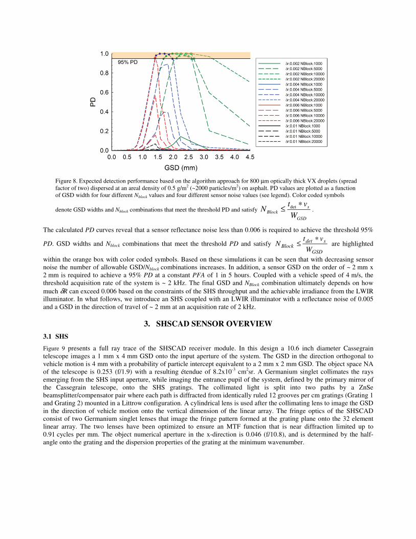
Figure 8. Expected detection performance based on the algorithm approach for 800 µm optically thick VX droplets (spread

factor of two) dispersed at an areal density of 0.5 g/m2 (~2000 particles/m2) on asphalt. PD values are plotted as a function

of GSD width for four different Nblock values and four different sensor noise values (see legend). Color coded symbols

denote GSD widths and Nblock combinations that meet the threshold PD and satisfy

GSD

sBlock

W

vtN

∗≤ det

.

The calculated PD curves reveal that a sensor reflectance noise less than 0.006 is required to achieve the threshold 95%

PD. GSD widths and Nblock combinations that meet the threshold PD and satisfy

GSD

sdetBlock

W

vtN

∗≤ are highlighted

within the orange box with color coded symbols. Based on these simulations it can be seen that with decreasing sensor

noise the number of allowable GSD/Nblock combinations increases. In addition, a sensor GSD on the order of ~ 2 mm x

2 mm is required to achieve a 95% PD at a constant PFA of 1 in 5 hours. Coupled with a vehicle speed of 4 m/s, the

threshold acquisition rate of the system is ~ 2 kHz. The final GSD and NBlock combination ultimately depends on how

much δR can exceed 0.006 based on the constraints of the SHS throughput and the achievable irradiance from the LWIR

illuminator. In what follows, we introduce an SHS coupled with an LWIR illuminator with a reflectance noise of 0.005

and a GSD in the direction of travel of ~ 2 mm at an acquisition rate of 2 kHz.

3. SHSCAD SENSOR OVERVIEW

3.1 SHS

Figure 9 presents a full ray trace of the SHSCAD receiver module. In this design a 10.6 inch diameter Cassegrain

telescope images a 1 mm x 4 mm GSD onto the input aperture of the system. The GSD in the direction orthogonal to

vehicle motion is 4 mm with a probability of particle intercept equivalent to a 2 mm x 2 mm GSD. The object space NA

of the telescope is 0.253 (f/1.9) with a resulting étendue of 8.2x10-3

cm2sr. A Germanium singlet collimates the rays

emerging from the SHS input aperture, while imaging the entrance pupil of the system, defined by the primary mirror of

the Cassegrain telescope, onto the SHS gratings. The collimated light is split into two paths by a ZnSe

beamsplitter/compensator pair where each path is diffracted from identically ruled 12 grooves per cm gratings (Grating 1

and Grating 2) mounted in a Littrow configuration. A cylindrical lens is used after the collimating lens to image the GSD

in the direction of vehicle motion onto the vertical dimension of the linear array. The fringe optics of the SHSCAD

consist of two Germanium singlet lenses that image the fringe pattern formed at the grating plane onto the 32 element

linear array. The two lenses have been optimized to ensure an MTF function that is near diffraction limited up to

0.91 cycles per mm. The object numerical aperture in the x-direction is 0.046 (f/10.8), and is determined by the half-

angle onto the grating and the dispersion properties of the grating at the minimum wavenumber.

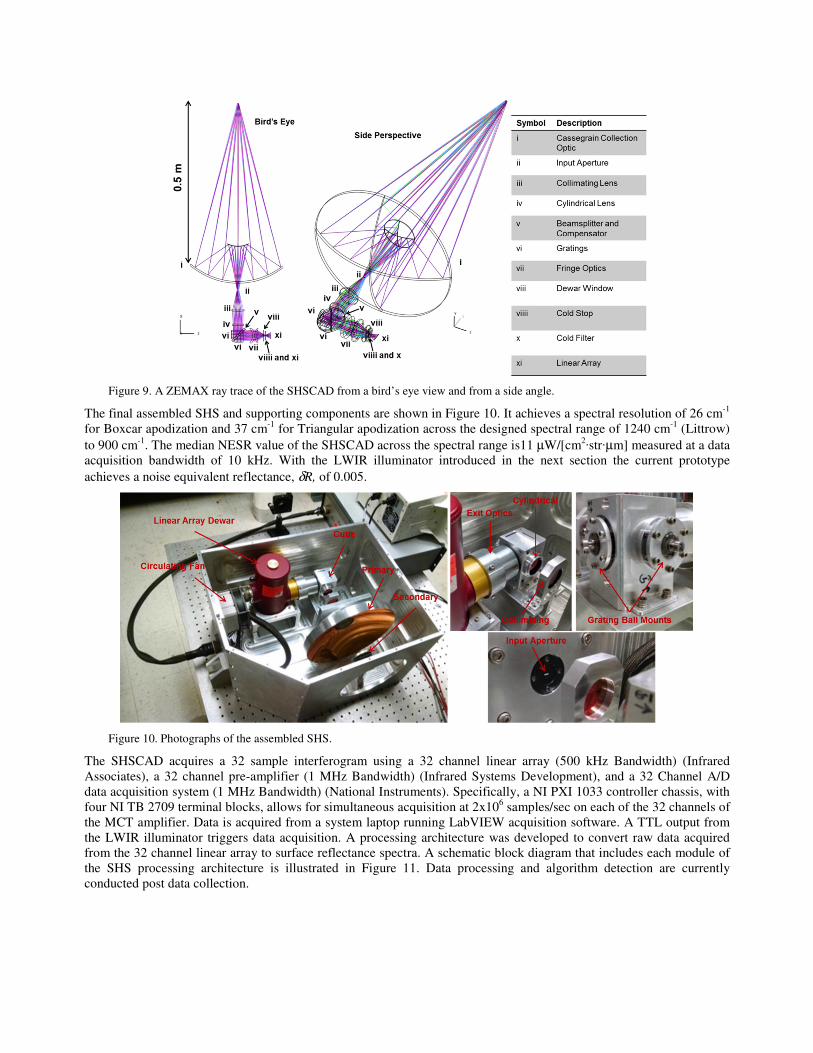
Figure 9. A ZEMAX ray trace of the SHSCAD from a bird’s eye view and from a side angle.

The final assembled SHS and supporting components are shown in Figure 10. It achieves a spectral resolution of 26 cm-1

for Boxcar apodization and 37 cm-1

for Triangular apodization across the designed spectral range of 1240 cm-1

(Littrow)

to 900 cm-1

. The median NESR value of the SHSCAD across the spectral range is11 µW/[cm2·str·µm] measured at a data

acquisition bandwidth of 10 kHz. With the LWIR illuminator introduced in the next section the current prototype

achieves a noise equivalent reflectance, δR, of 0.005.

Figure 10. Photographs of the assembled SHS.

The SHSCAD acquires a 32 sample interferogram using a 32 channel linear array (500 kHz Bandwidth) (Infrared

Associates), a 32 channel pre-amplifier (1 MHz Bandwidth) (Infrared Systems Development), and a 32 Channel A/D

data acquisition system (1 MHz Bandwidth) (National Instruments). Specifically, a NI PXI 1033 controller chassis, with

four NI TB 2709 terminal blocks, allows for simultaneous acquisition at 2x106 samples/sec on each of the 32 channels of

the MCT amplifier. Data is acquired from a system laptop running LabVIEW acquisition software. A TTL output from

the LWIR illuminator triggers data acquisition. A processing architecture was developed to convert raw data acquired

from the 32 channel linear array to surface reflectance spectra. A schematic block diagram that includes each module of

the SHS processing architecture is illustrated in Figure 11. Data processing and algorithm detection are currently

conducted post data collection.

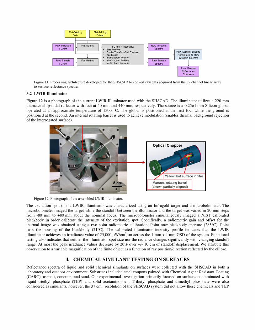
Figure 11. Processing architecture developed for the SHSCAD to convert raw data acquired from the 32 channel linear array

to surface reflectance spectra.

3.2 LWIR Illuminator

Figure 12 is a photograph of the current LWIR Illuminator used with the SHSCAD. The illuminator utilizes a 220 mm

diameter ellipsoidal reflector with foci at 40 mm and 440 mm, respectively. The source is a 0.25×1 mm Silicon globar

operated at an approximate temperature of 1300° C. The globar is positioned at the first foci while the ground is

positioned at the second. An internal rotating barrel is used to achieve modulation (enables thermal background rejection

of the interrogated surface).

Figure 12. Photograph of the assembled LWIR Illuminator.

The excitation spot of the LWIR illuminator was characterized using an Infragold target and a microbolometer. The

microbolometer imaged the target while the standoff between the illuminator and the target was varied in 20 mm steps

from -80 mm to +80 mm about the nominal focus. The microbolometer simultaneously imaged a NIST calibrated

blackbody in order calibrate the intensity of the excitation spot. Specifically, a radiometric gain and offset for the

thermal image was obtained using a two-point radiometric calibration; Point one: blackbody aperture (285°C); Point

two: the housing of the blackbody (21°C). The calibrated illuminator intensity profile indicates that the LWIR

illuminator achieves an irradiance value of 25,000 µW/cm2µm across the 1 mm x 4 mm GSD of the system. Functional

testing also indicates that neither the illuminator spot size nor the radiance changes significantly with changing standoff

range. At most the peak irradiance values decrease by 20% over +/- 10 cm of standoff displacement. We attribute this

observation to a variable magnification of the finite object as a function of ray position/direction reflected by the ellipse.

4. CHEMICAL SIMULANT TESTING ON SURFACES

Reflectance spectra of liquid and solid chemical simulants on surfaces were collected with the SHSCAD in both a

laboratory and outdoor environment. Substrates included steel coupons painted with Chemical Agent Resistant Coating

(CARC), asphalt, concrete, and sand. Our experimental investigation primarily focused on surfaces contaminated with

liquid triethyl phosphate (TEP) and solid acetaminophen. Tributyl phosphate and dimethyl phosphate were also

considered as simulants, however, the 37 cm-1

resolution of the SHSCAD system did not allow these chemicals and TEP

to be discriminated. Methyl ethyl salicylate (MES) was also identified as a simulant. However, the discriminate

reflectance features of liquid MES are below the reflectance noise of the system.

Substrates dosed with liquid TEP were prepared using an Eppendorf Research Plus (0.1-2.5 µl) pipette to drop cast

0.30 µl of fluid (equivalent to a particle diameter of 800 µm). The mean droplet mass dispensed by the pipette was

0.325 µg with a standard deviation of 0.124 µg (based on 20 droplets measured using a Cahn C-30 microbalance).

Substrates dosed with solid acetaminophen were prepared by weighing a known mass and sifting the powder through a

sieve with 500 µm openings over a known area.

4.1 Indoor testing overview

Reflectance spectra of simulants dosed on surfaces were collected in an indoor laboratory to characterize per sample

probability of detection (pd) for a per sample probability of false alarm (pfa) of 1%. We should point out that the pfa

values reported below are based only on false alarms against the uncontaminated surface. They do not consider

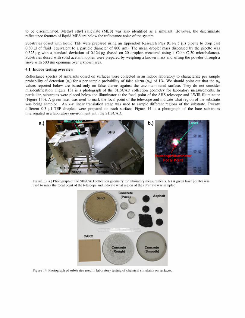
misidentification. Figure 13a is a photograph of the SHSCAD collection geometry for laboratory measurements. In

particular, substrates were placed below the illuminator at the focal point of the SHS telescope and LWIR illuminator

(Figure 13b). A green laser was used to mark the focal point of the telescope and indicate what region of the substrate

was being sampled. An x-y linear translation stage was used to sample different regions of the substrate. Twenty

different 0.3 µl TEP droplets were prepared on each surface. Figure 14 is a photograph of the bare substrates

interrogated in a laboratory environment with the SHSCAD.

Figure 13. a.) Photograph of the SHSCAD collection geometry for laboratory measurements. b.) A green laser pointer was

used to mark the focal point of the telescope and indicate what region of the substrate was sampled.

Figure 14. Photograph of substrates used in laboratory testing of chemical simulants on surfaces.

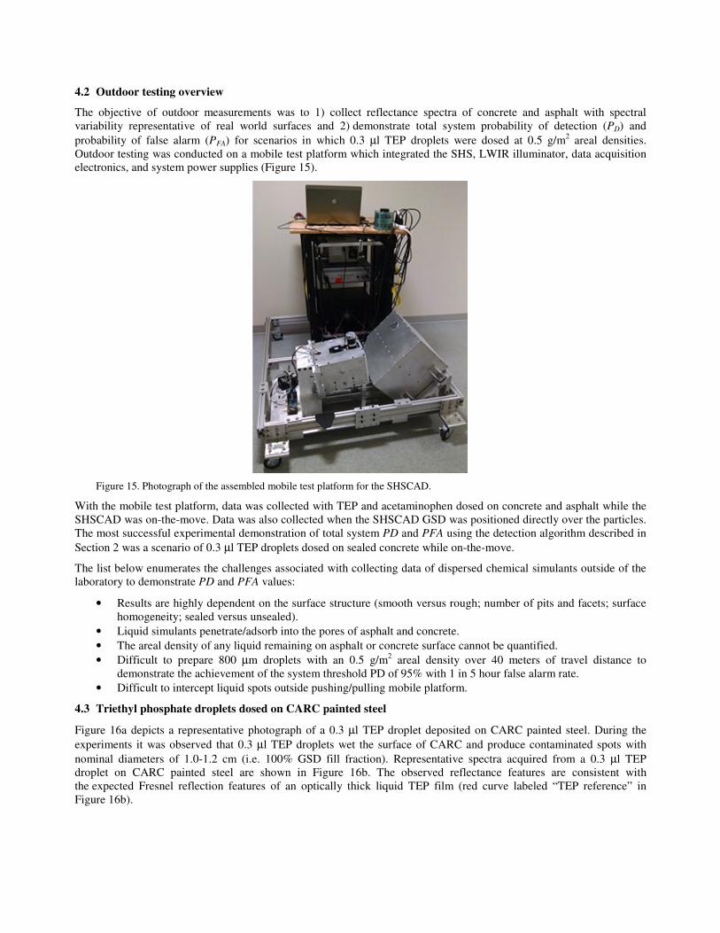
4.2 Outdoor testing overview

The objective of outdoor measurements was to 1) collect reflectance spectra of concrete and asphalt with spectral

variability representative of real world surfaces and 2) demonstrate total system probability of detection (PD) and

probability of false alarm (PFA) for scenarios in which 0.3 µl TEP droplets were dosed at 0.5 g/m2 areal densities.

Outdoor testing was conducted on a mobile test platform which integrated the SHS, LWIR illuminator, data acquisition

electronics, and system power supplies (Figure 15).

Figure 15. Photograph of the assembled mobile test platform for the SHSCAD.

With the mobile test platform, data was collected with TEP and acetaminophen dosed on concrete and asphalt while the

SHSCAD was on-the-move. Data was also collected when the SHSCAD GSD was positioned directly over the particles.

The most successful experimental demonstration of total system PD and PFA using the detection algorithm described in

Section 2 was a scenario of 0.3 µl TEP droplets dosed on sealed concrete while on-the-move.

The list below enumerates the challenges associated with collecting data of dispersed chemical simulants outside of the

laboratory to demonstrate PD and PFA values:

• Results are highly dependent on the surface structure (smooth versus rough; number of pits and facets; surface

homogeneity; sealed versus unsealed).

• Liquid simulants penetrate/adsorb into the pores of asphalt and concrete.

• The areal density of any liquid remaining on asphalt or concrete surface cannot be quantified.

• Difficult to prepare 800 µm droplets with an 0.5 g/m2 areal density over 40 meters of travel distance to

demonstrate the achievement of the system threshold PD of 95% with 1 in 5 hour false alarm rate.

• Difficult to intercept liquid spots outside pushing/pulling mobile platform.

4.3 Triethyl phosphate droplets dosed on CARC painted steel

Figure 16a depicts a representative photograph of a 0.3 µl TEP droplet deposited on CARC painted steel. During the

experiments it was observed that 0.3 µl TEP droplets wet the surface of CARC and produce contaminated spots with

nominal diameters of 1.0-1.2 cm (i.e. 100% GSD fill fraction). Representative spectra acquired from a 0.3 µl TEP

droplet on CARC painted steel are shown in Figure 16b. The observed reflectance features are consistent with

the expected Fresnel reflection features of an optically thick liquid TEP film (red curve labeled “TEP reference” in

Figure 16b).

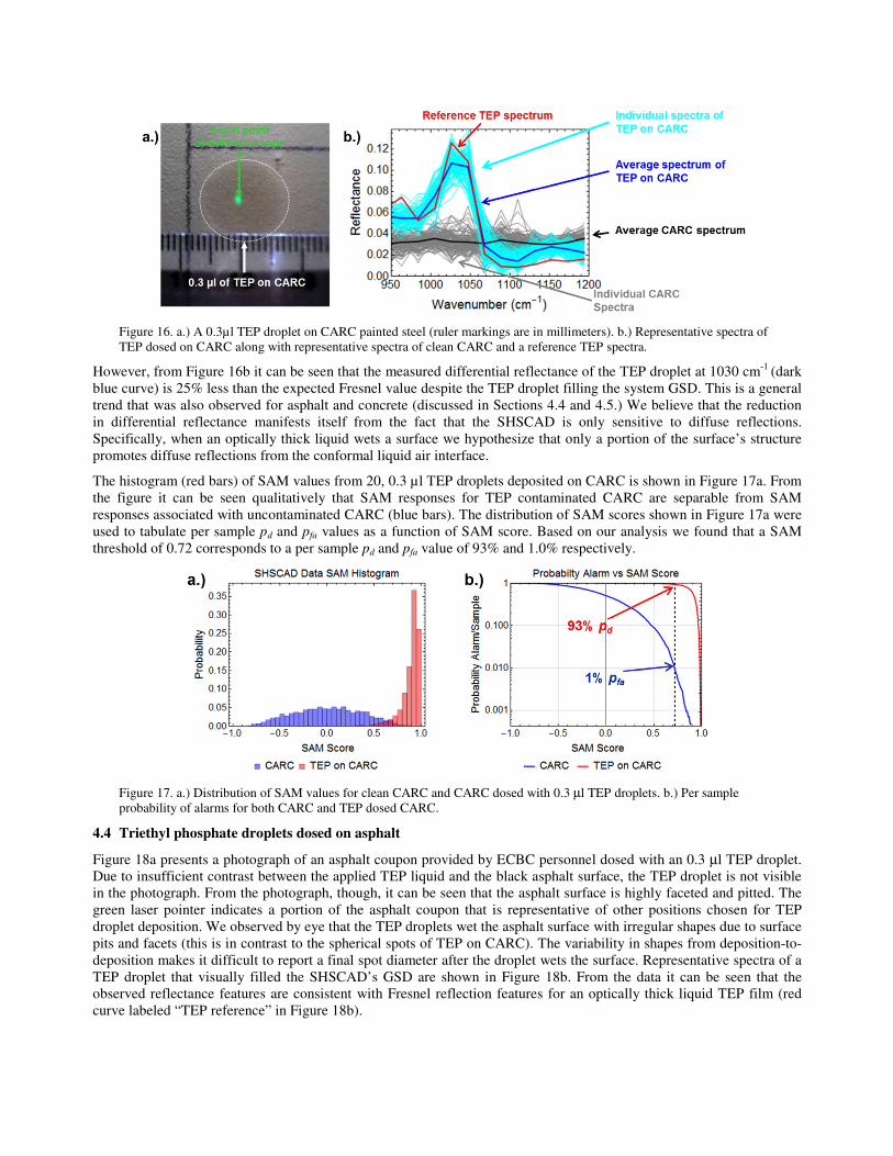
Figure 16. a.) A 0.3µl TEP droplet on CARC painted steel (ruler markings are in millimeters). b.) Representative spectra of

TEP dosed on CARC along with representative spectra of clean CARC and a reference TEP spectra.

However, from Figure 16b it can be seen that the measured differential reflectance of the TEP droplet at 1030 cm-1

(dark

blue curve) is 25% less than the expected Fresnel value despite the TEP droplet filling the system GSD. This is a general

trend that was also observed for asphalt and concrete (discussed in Sections 4.4 and 4.5.) We believe that the reduction

in differential reflectance manifests itself from the fact that the SHSCAD is only sensitive to diffuse reflections.

Specifically, when an optically thick liquid wets a surface we hypothesize that only a portion of the surface’s structure

promotes diffuse reflections from the conformal liquid air interface.

The histogram (red bars) of SAM values from 20, 0.3 µl TEP droplets deposited on CARC is shown in Figure 17a. From

the figure it can be seen qualitatively that SAM responses for TEP contaminated CARC are separable from SAM

responses associated with uncontaminated CARC (blue bars). The distribution of SAM scores shown in Figure 17a were

used to tabulate per sample pd and pfa values as a function of SAM score. Based on our analysis we found that a SAM

threshold of 0.72 corresponds to a per sample pd and pfa value of 93% and 1.0% respectively.

Figure 17. a.) Distribution of SAM values for clean CARC and CARC dosed with 0.3 µl TEP droplets. b.) Per sample

probability of alarms for both CARC and TEP dosed CARC.

4.4 Triethyl phosphate droplets dosed on asphalt

Figure 18a presents a photograph of an asphalt coupon provided by ECBC personnel dosed with an 0.3 µl TEP droplet.

Due to insufficient contrast between the applied TEP liquid and the black asphalt surface, the TEP droplet is not visible

in the photograph. From the photograph, though, it can be seen that the asphalt surface is highly faceted and pitted. The

green laser pointer indicates a portion of the asphalt coupon that is representative of other positions chosen for TEP

droplet deposition. We observed by eye that the TEP droplets wet the asphalt surface with irregular shapes due to surface

pits and facets (this is in contrast to the spherical spots of TEP on CARC). The variability in shapes from deposition-to-

deposition makes it difficult to report a final spot diameter after the droplet wets the surface. Representative spectra of a

TEP droplet that visually filled the SHSCAD’s GSD are shown in Figure 18b. From the data it can be seen that the

observed reflectance features are consistent with Fresnel reflection features for an optically thick liquid TEP film (red

curve labeled “TEP reference” in Figure 18b).

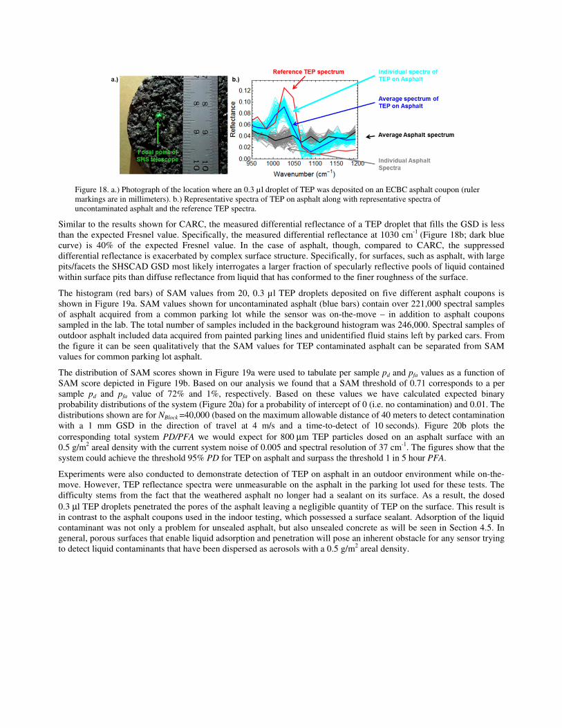
Figure 18. a.) Photograph of the location where an 0.3 µl droplet of TEP was deposited on an ECBC asphalt coupon (ruler

markings are in millimeters). b.) Representative spectra of TEP on asphalt along with representative spectra of

uncontaminated asphalt and the reference TEP spectra.

Similar to the results shown for CARC, the measured differential reflectance of a TEP droplet that fills the GSD is less

than the expected Fresnel value. Specifically, the measured differential reflectance at 1030 cm-1

(Figure 18b; dark blue

curve) is 40% of the expected Fresnel value. In the case of asphalt, though, compared to CARC, the suppressed

differential reflectance is exacerbated by complex surface structure. Specifically, for surfaces, such as asphalt, with large

pits/facets the SHSCAD GSD most likely interrogates a larger fraction of specularly reflective pools of liquid contained

within surface pits than diffuse reflectance from liquid that has conformed to the finer roughness of the surface.

The histogram (red bars) of SAM values from 20, 0.3 µl TEP droplets deposited on five different asphalt coupons is

shown in Figure 19a. SAM values shown for uncontaminated asphalt (blue bars) contain over 221,000 spectral samples

of asphalt acquired from a common parking lot while the sensor was on-the-move – in addition to asphalt coupons

sampled in the lab. The total number of samples included in the background histogram was 246,000. Spectral samples of

outdoor asphalt included data acquired from painted parking lines and unidentified fluid stains left by parked cars. From

the figure it can be seen qualitatively that the SAM values for TEP contaminated asphalt can be separated from SAM

values for common parking lot asphalt.

The distribution of SAM scores shown in Figure 19a were used to tabulate per sample pd and pfa values as a function of

SAM score depicted in Figure 19b. Based on our analysis we found that a SAM threshold of 0.71 corresponds to a per

sample pd and pfa value of 72% and 1%, respectively. Based on these values we have calculated expected binary

probability distributions of the system (Figure 20a) for a probability of intercept of 0 (i.e. no contamination) and 0.01. The

distributions shown are for NBlock =40,000 (based on the maximum allowable distance of 40 meters to detect contamination

with a 1 mm GSD in the direction of travel at 4 m/s and a time-to-detect of 10 seconds). Figure 20b plots the

corresponding total system PD/PFA we would expect for 800 µm TEP particles dosed on an asphalt surface with an

0.5 g/m2 areal density with the current system noise of 0.005 and spectral resolution of 37 cm

-1. The figures show that the

system could achieve the threshold 95% PD for TEP on asphalt and surpass the threshold 1 in 5 hour PFA.

Experiments were also conducted to demonstrate detection of TEP on asphalt in an outdoor environment while on-the-

move. However, TEP reflectance spectra were unmeasurable on the asphalt in the parking lot used for these tests. The

difficulty stems from the fact that the weathered asphalt no longer had a sealant on its surface. As a result, the dosed

0.3 µl TEP droplets penetrated the pores of the asphalt leaving a negligible quantity of TEP on the surface. This result is

in contrast to the asphalt coupons used in the indoor testing, which possessed a surface sealant. Adsorption of the liquid

contaminant was not only a problem for unsealed asphalt, but also unsealed concrete as will be seen in Section 4.5. In

general, porous surfaces that enable liquid adsorption and penetration will pose an inherent obstacle for any sensor trying

to detect liquid contaminants that have been dispersed as aerosols with a 0.5 g/m2 areal density.

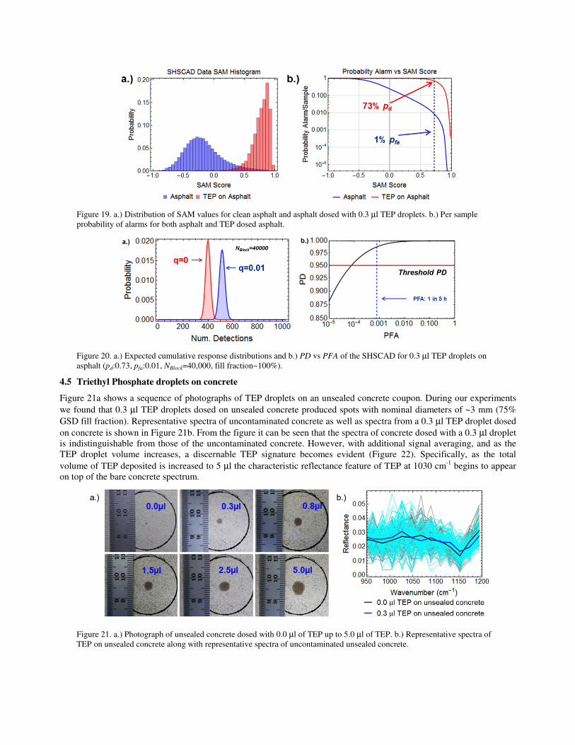
Figure 19. a.) Distribution of SAM values for clean asphalt and asphalt dosed with 0.3 µl TEP droplets. b.) Per sample

probability of alarms for both asphalt and TEP dosed asphalt.

Figure 20. a.) Expected cumulative response distributions and b.) PD vs PFA of the SHSCAD for 0.3 µl TEP droplets on

asphalt (pd:0.73, pfa:0.01, NBlock=40,000, fill fraction~100%).

4.5 Triethyl Phosphate droplets on concrete

Figure 21a shows a sequence of photographs of TEP droplets on an unsealed concrete coupon. During our experiments

we found that 0.3 µl TEP droplets dosed on unsealed concrete produced spots with nominal diameters of ~3 mm (75%

GSD fill fraction). Representative spectra of uncontaminated concrete as well as spectra from a 0.3 µl TEP droplet dosed

on concrete is shown in Figure 21b. From the figure it can be seen that the spectra of concrete dosed with a 0.3 µl droplet

is indistinguishable from those of the uncontaminated concrete. However, with additional signal averaging, and as the

TEP droplet volume increases, a discernable TEP signature becomes evident (Figure 22). Specifically, as the total

volume of TEP deposited is increased to 5 µl the characteristic reflectance feature of TEP at 1030 cm-1

begins to appear

on top of the bare concrete spectrum.

Figure 21. a.) Photograph of unsealed concrete dosed with 0.0 µl of TEP up to 5.0 µl of TEP. b.) Representative spectra of

TEP on unsealed concrete along with representative spectra of uncontaminated unsealed concrete.

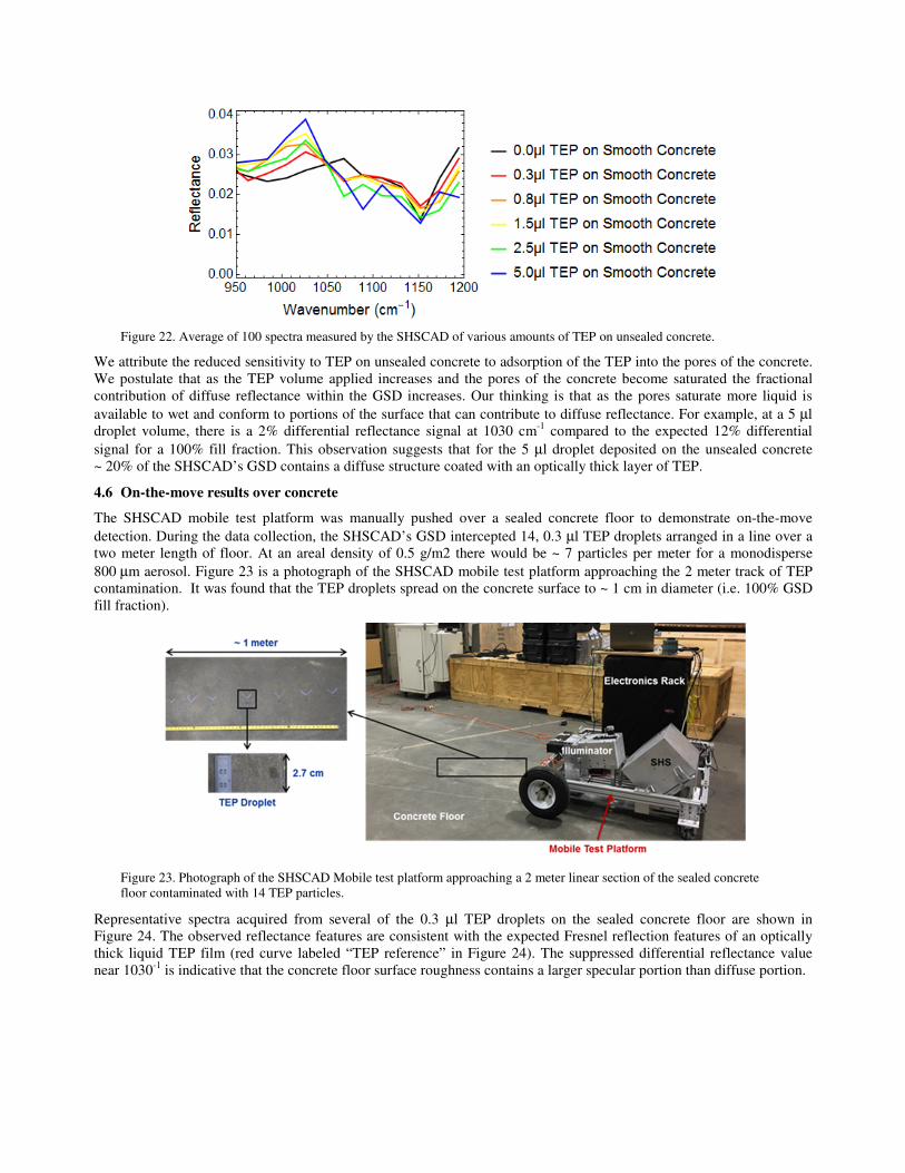
Figure 22. Average of 100 spectra measured by the SHSCAD of various amounts of TEP on unsealed concrete.

We attribute the reduced sensitivity to TEP on unsealed concrete to adsorption of the TEP into the pores of the concrete.

We postulate that as the TEP volume applied increases and the pores of the concrete become saturated the fractional

contribution of diffuse reflectance within the GSD increases. Our thinking is that as the pores saturate more liquid is

available to wet and conform to portions of the surface that can contribute to diffuse reflectance. For example, at a 5 µl

droplet volume, there is a 2% differential reflectance signal at 1030 cm-1

compared to the expected 12% differential

signal for a 100% fill fraction. This observation suggests that for the 5 µl droplet deposited on the unsealed concrete

~ 20% of the SHSCAD’s GSD contains a diffuse structure coated with an optically thick layer of TEP.

4.6 On-the-move results over concrete

The SHSCAD mobile test platform was manually pushed over a sealed concrete floor to demonstrate on-the-move

detection. During the data collection, the SHSCAD’s GSD intercepted 14, 0.3 µl TEP droplets arranged in a line over a

two meter length of floor. At an areal density of 0.5 g/m2 there would be ~ 7 particles per meter for a monodisperse

800 µm aerosol. Figure 23 is a photograph of the SHSCAD mobile test platform approaching the 2 meter track of TEP

contamination. It was found that the TEP droplets spread on the concrete surface to ~ 1 cm in diameter (i.e. 100% GSD

fill fraction).

Figure 23. Photograph of the SHSCAD Mobile test platform approaching a 2 meter linear section of the sealed concrete

floor contaminated with 14 TEP particles.

Representative spectra acquired from several of the 0.3 µl TEP droplets on the sealed concrete floor are shown in

Figure 24. The observed reflectance features are consistent with the expected Fresnel reflection features of an optically

thick liquid TEP film (red curve labeled “TEP reference” in Figure 24). The suppressed differential reflectance value

near 1030-1

is indicative that the concrete floor surface roughness contains a larger specular portion than diffuse portion.

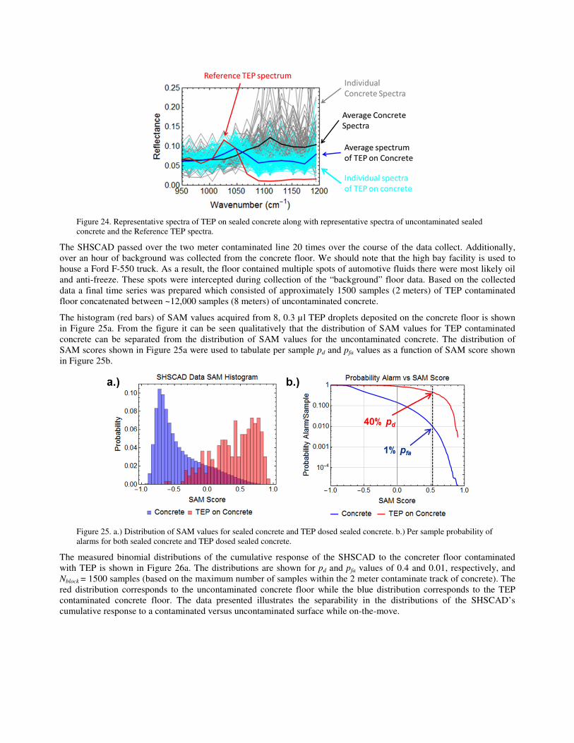
Figure 24. Representative spectra of TEP on sealed concrete along with representative spectra of uncontaminated sealed

concrete and the Reference TEP spectra.

The SHSCAD passed over the two meter contaminated line 20 times over the course of the data collect. Additionally,

over an hour of background was collected from the concrete floor. We should note that the high bay facility is used to

house a Ford F-550 truck. As a result, the floor contained multiple spots of automotive fluids there were most likely oil

and anti-freeze. These spots were intercepted during collection of the “background” floor data. Based on the collected

data a final time series was prepared which consisted of approximately 1500 samples (2 meters) of TEP contaminated

floor concatenated between ~12,000 samples (8 meters) of uncontaminated concrete.

The histogram (red bars) of SAM values acquired from 8, 0.3 µl TEP droplets deposited on the concrete floor is shown

in Figure 25a. From the figure it can be seen qualitatively that the distribution of SAM values for TEP contaminated

concrete can be separated from the distribution of SAM values for the uncontaminated concrete. The distribution of

SAM scores shown in Figure 25a were used to tabulate per sample pd and pfa values as a function of SAM score shown

in Figure 25b.

Figure 25. a.) Distribution of SAM values for sealed concrete and TEP dosed sealed concrete. b.) Per sample probability of

alarms for both sealed concrete and TEP dosed sealed concrete.

The measured binomial distributions of the cumulative response of the SHSCAD to the concreter floor contaminated

with TEP is shown in Figure 26a. The distributions are shown for pd and pfa values of 0.4 and 0.01, respectively, and

Nblock = 1500 samples (based on the maximum number of samples within the 2 meter contaminate track of concrete). The

red distribution corresponds to the uncontaminated concrete floor while the blue distribution corresponds to the TEP

contaminated concrete floor. The data presented illustrates the separability in the distributions of the SHSCAD’s

cumulative response to a contaminated versus uncontaminated surface while on-the-move.

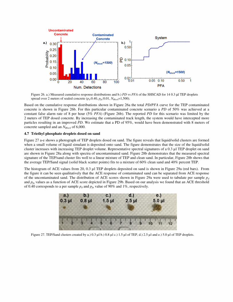
Figure 26. a.) Measured cumulative response distributions and b.) PD vs PFA of the SHSCAD for 14 0.3 µl TEP droplets

spread over 2 meters of sealed concrete (pd:0.40, pfa:0.01, NBlock=1,500).

Based on the cumulative response distributions shown in Figure 26a the total PD/PFA curve for the TEP contaminated

concrete is shown in Figure 26b. For this particular contaminated concrete scenario a PD of 50% was achieved at a

constant false alarm rate of 8 per hour (5% PFA) (Figure 26b). The reported PD for this scenario was limited by the

2 meters of TEP dosed concrete. By increasing the contaminated track length, the system would have intercepted more

particles resulting in an improved PD. We estimate that a PD of 95%, would have been demonstrated with 8 meters of

concrete sampled and an NBlock of 6,000.

4.7 Triethyl phosphate droplets dosed on sand

Figure 27 a-e shows a photograph of TEP droplets dosed on sand. The figure reveals that liquid/solid clusters are formed

when a small volume of liquid simulant is deposited onto sand. The figure demonstrates that the size of the liquid/solid

cluster increases with increasing TEP droplet volume. Representative spectral signatures of a 0.3 µl TEP droplet on sand

are shown in Figure 28a along with spectra of uncontaminated sand. Figure 28b demonstrates that the measured spectral

signature of the TEP/sand cluster fits well to a linear mixture of TEP and clean sand. In particular, Figure 28b shows that

the average TEP/Sand signal (solid black scatter points) fits to a mixture of 60% clean sand and 40% percent TEP.

The histogram of ACE values from 20, 0.3 µl TEP droplets deposited on sand is shown in Figure 29a (red bars). From

the figure it can be seen qualitatively that the ACE response of contaminated sand can be separated from ACE response

of the uncontaminated sand. The distribution of ACE scores shown in Figure 29a were used to tabulate per sample pd

and pfa values as a function of ACE score depicted in Figure 29b. Based on our analysis we found that an ACE threshold

of 0.40 corresponds to a per sample pd and pfa value of 90% and 1%, respectively.

Figure 27. TEP/Sand clusters created by a.) 0.3 µl b.) 0.8 µl c.) 1.5 µl of TEP, d.) 2.5 µl and e.) 5.0 µl of TEP droplets.

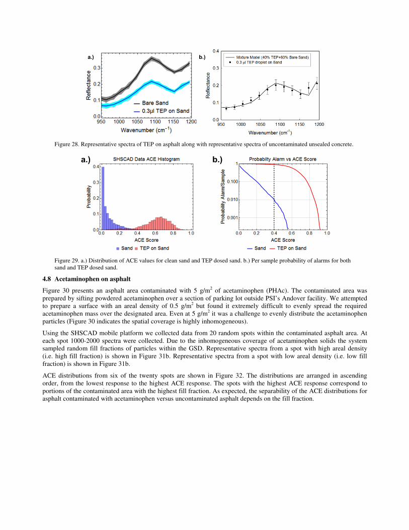
Figure 28. Representative spectra of TEP on asphalt along with representative spectra of uncontaminated unsealed concrete.

Figure 29. a.) Distribution of ACE values for clean sand and TEP dosed sand. b.) Per sample probability of alarms for both

sand and TEP dosed sand.

4.8 Acetaminophen on asphalt

Figure 30 presents an asphalt area contaminated with 5 g/m2 of acetaminophen (PHAc). The contaminated area was

prepared by sifting powdered acetaminophen over a section of parking lot outside PSI’s Andover facility. We attempted

to prepare a surface with an areal density of 0.5 g/m2 but found it extremely difficult to evenly spread the required

acetaminophen mass over the designated area. Even at 5 g/m2 it was a challenge to evenly distribute the acetaminophen

particles (Figure 30 indicates the spatial coverage is highly inhomogeneous).

Using the SHSCAD mobile platform we collected data from 20 random spots within the contaminated asphalt area. At

each spot 1000-2000 spectra were collected. Due to the inhomogeneous coverage of acetaminophen solids the system

sampled random fill fractions of particles within the GSD. Representative spectra from a spot with high areal density

(i.e. high fill fraction) is shown in Figure 31b. Representative spectra from a spot with low areal density (i.e. low fill

fraction) is shown in Figure 31b.

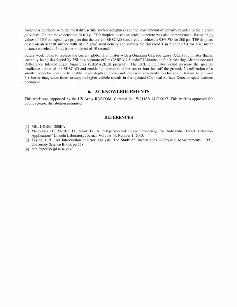
ACE distributions from six of the twenty spots are shown in Figure 32. The distributions are arranged in ascending

order, from the lowest response to the highest ACE response. The spots with the highest ACE response correspond to

portions of the contaminated area with the highest fill fraction. As expected, the separability of the ACE distributions for

asphalt contaminated with acetaminophen versus uncontaminated asphalt depends on the fill fraction.

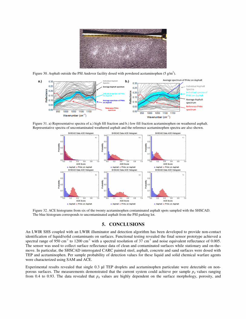
Figure 30. Asphalt outside the PSI Andover facility dosed with powdered acetaminophen (5 g/m2).

Figure 31. a) Representative spectra of a.) high fill fraction and b.) low fill fraction acetaminophen on weathered asphalt.

Representative spectra of uncontaminated weathered asphalt and the reference acetaminophen spectra are also shown.

Figure 32. ACE histograms from six of the twenty acetaminophen contaminated asphalt spots sampled with the SHSCAD.

The blue histogram corresponds to uncontaminated asphalt from the PSI parking lot.

5. CONCLUSIONS

An LWIR SHS coupled with an LWIR illuminator and detection algorithm has been developed to provide non-contact

identification of liquid/solid contaminants on surfaces. Functional testing revealed the final sensor prototype achieved a

spectral range of 950 cm-1

to 1200 cm-1

with a spectral resolution of 37 cm-1

and noise equivalent reflectance of 0.005.

The sensor was used to collect surface reflectance data of clean and contaminated surfaces while stationary and on-the-

move. In particular, the SHSCAD interrogated CARC painted steel, asphalt, concrete and sand surfaces were dosed with

TEP and acetaminophen. Per sample probability of detection values for these liquid and solid chemical warfare agents

were characterized using SAM and ACE.

Experimental results revealed that single 0.3 µl TEP droplets and acetaminophen particulate were detectable on non-

porous surfaces. The measurements demonstrated that the current system could achieve per sample pd values ranging

from 0.4 to 0.93. The data revealed that pd values are highly dependent on the surface morphology, porosity, and

roughness. Surfaces with the most diffuse like surface roughness and the least amount of porosity resulted in the highest

pd values. On the move detection of 0.3 µl TEP droplets dosed on sealed concrete was also demonstrated. Based on pd

values of TEP on asphalt we project that the current SHSCAD sensor could achieve a 95% PD for 800 µm TEP droplets

dosed on an asphalt surface with an 0.5 g/m2 areal density and surpass the threshold 1 in 5 hour PFA for a 40 meter

distance traveled at 4 m/s (time-to-detect of 10 seconds).

Future work looks to replace the current globar illuminator with a Quantum Cascade Laser (QCL) illuminator that is

currently being developed by PSI in a separate effort (IARPA’s Standoff ILluminator for Measuring Absorbance and

Reflectance Infrared Light Signatures (SILMARILS) program). The QCL illuminator would increase the spectral

irradiance output of the SHSCAD and enable 1.) operation of the sensor four feet off the ground, 2.) utilization of a

smaller collector aperture to enable larger depth of focus and improved sensitivity to changes in terrain height and

3.) shorter integration times to support higher vehicle speeds in the updated Chemical Surface Detector specifications

document.

6. ACKNOWLEDGEMENTS

This work was supported by the US Army RDECOM, Contract No. W911SR-14-C-0017. This work is approved for

public release; distribution unlimited.

REFERENCES

[1] MIL-HDBK-1200EA

[2] Manolakis D.; Marden D.; Shaw G. A. “Hyperspectral Image Processing for Automatic Target Detection

Applications” Lincoln Laboratory Journal, Volume 14, Number 1, 2003.

[3] Taylor, J. R. “An Introduction to Error Analysis. The Study of Uncertainties in Physical Measurements” 1997,

University Science Books pp 228.

[4] http://speclib.jpl.nasa.gov/