Advanced Engineering Mathematics, 10/e by Edwin Kreyszig Copyright 2011 by John Wiley & Sons. All...
78
Advanced Engineering Mathematics, 10/e by Edwin Kreyszig Copyright 2011 by John Wiley & Sons. All rights reserved. CHAPTER 8 Linear Algebra: Matrix Eigenvalue Problems Chapter 8 p1
-
Upload
samuel-johns -
Category
Documents
-
view
239 -
download
0
Transcript of Advanced Engineering Mathematics, 10/e by Edwin Kreyszig Copyright 2011 by John Wiley & Sons. All...
Advanced Engineering Mathematics, 10/e by Edwin KreyszigCopyright 2011 by John Wiley & Sons. All rights reserved.
CHAPTER 8Linear Algebra:
Matrix Eigenvalue Problems
Chapter 8 p1
Advanced Engineering Mathematics, 10/e by Edwin KreyszigCopyright 2011 by John Wiley & Sons. All rights reserved.
Section 8.0 p2
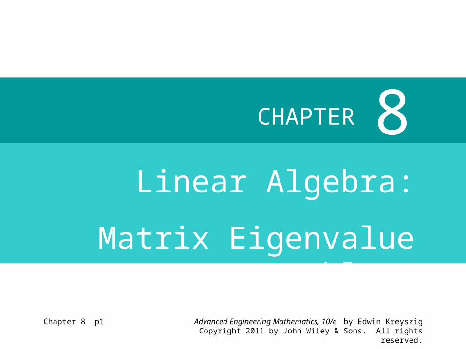
A matrix eigenvalue problem considers the vector equation
(1) Ax = λx.
Here A is a given square matrix, λ an unknown scalar, and x an unknown vector. In a matrix eigenvalue problem, the task is to determine λ’s and x’s that satisfy (1).
Since x = 0 is always a solution for any and thus not interesting, we only admit solutions with x ≠ 0.
The solutions to (1) are given the following names: The λ’s that satisfy (1) are called eigenvalues of A and the corresponding nonzero x’s that also satisfy (1) are called eigenvectors of A.
8.0 Linear Algebra: Matrix Eigenvalue Problems
Advanced Engineering Mathematics, 10/e by Edwin KreyszigCopyright 2011 by John Wiley & Sons. All rights reserved.
Section 8.1 p3
8.1 The Matrix Eigenvalue Problem. Determining
Eigenvalues and Eigenvectors
8.1 The Matrix Eigenvalue Problem. Determining
Eigenvalues and Eigenvectors

Advanced Engineering Mathematics, 10/e by Edwin KreyszigCopyright 2011 by John Wiley & Sons. All rights reserved.
Section 8.1 p4
We formalize our observation. Let A = [ajk] be a given nonzero square matrix of dimension n × n. Consider the following vector equation:(1) Ax = λx.The problem of finding nonzero x’s and λ’s that satisfy equation (1) is called an eigenvalue problem.
We formalize our observation. Let A = [ajk] be a given nonzero square matrix of dimension n × n. Consider the following vector equation:(1) Ax = λx.The problem of finding nonzero x’s and λ’s that satisfy equation (1) is called an eigenvalue problem.
8.1 The Matrix Eigenvalue Problem. DeterminingEigenvalues and Eigenvectors
Advanced Engineering Mathematics, 10/e by Edwin KreyszigCopyright 2011 by John Wiley & Sons. All rights reserved.
Section 8.1 p5
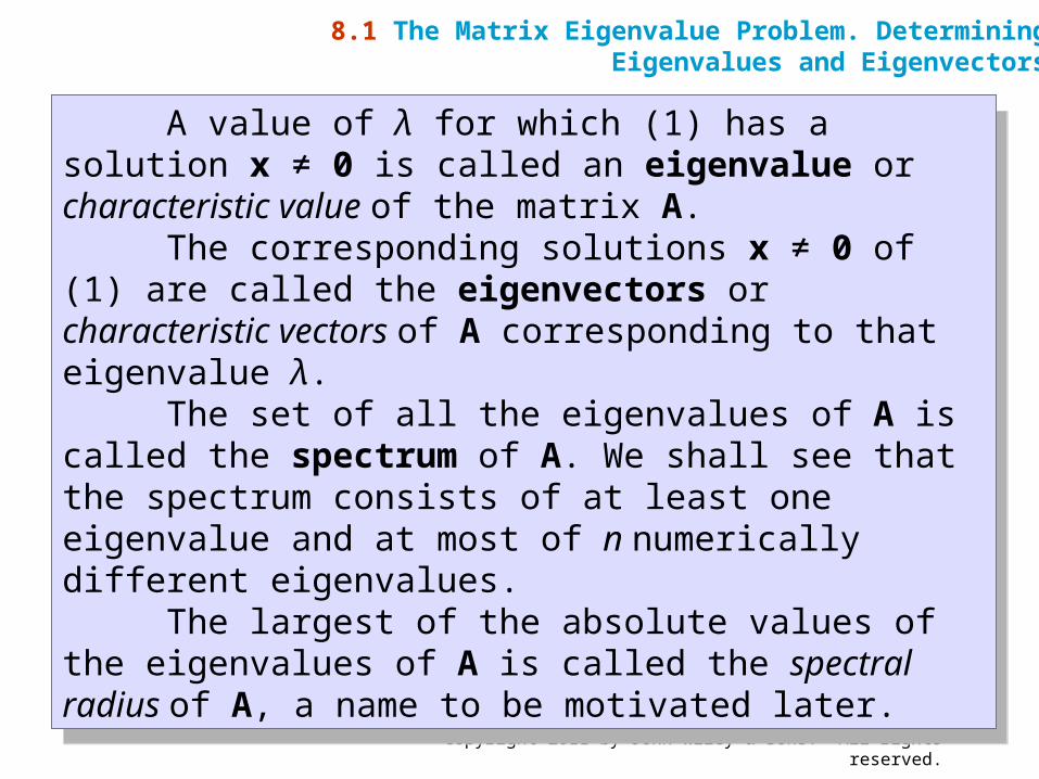
A value of λ for which (1) has a solution x ≠ 0 is called an eigenvalue or characteristic value of the matrix A.
The corresponding solutions x ≠ 0 of (1) are called the eigenvectors or characteristic vectors of A corresponding to that eigenvalue λ.
The set of all the eigenvalues of A is called the spectrum of A. We shall see that the spectrum consists of at least one eigenvalue and at most of n numerically different eigenvalues.
The largest of the absolute values of the eigenvalues of A is called the spectral radius of A, a name to be motivated later.
8.1 The Matrix Eigenvalue Problem. DeterminingEigenvalues and Eigenvectors
Advanced Engineering Mathematics, 10/e by Edwin KreyszigCopyright 2011 by John Wiley & Sons. All rights reserved.
Section 8.1 p6
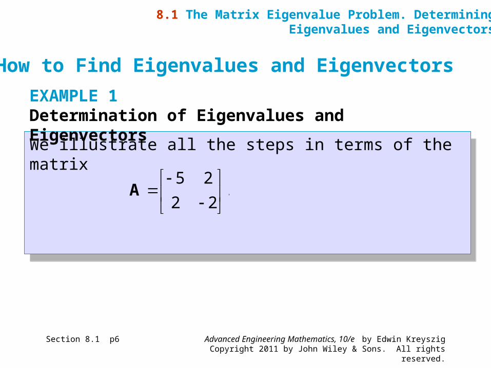
We illustrate all the steps in terms of the matrixWe illustrate all the steps in terms of the matrix
How to Find Eigenvalues and Eigenvectors
8.1 The Matrix Eigenvalue Problem. DeterminingEigenvalues and Eigenvectors
EXAMPLE 1 Determination of Eigenvalues and Eigenvectors
5 2.
2 2
A
Advanced Engineering Mathematics, 10/e by Edwin KreyszigCopyright 2011 by John Wiley & Sons. All rights reserved.
Section 8.1 p7
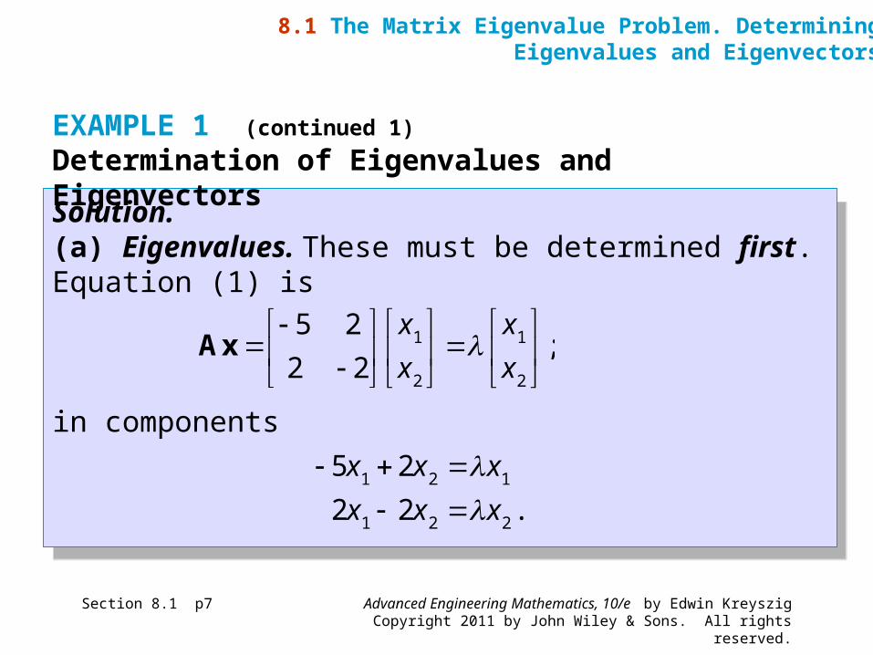
Solution. (a) Eigenvalues. These must be determined first. Equation (1) is
in components
Solution. (a) Eigenvalues. These must be determined first. Equation (1) is
in components
8.1 The Matrix Eigenvalue Problem. DeterminingEigenvalues and Eigenvectors
EXAMPLE 1 (continued 1) Determination of Eigenvalues and Eigenvectors
1 1
2 2
5 2;
2 2
x x
x x
Ax
1 2 1
1 2 2
5 2
2 2 .
x x x
x x x
Advanced Engineering Mathematics, 10/e by Edwin KreyszigCopyright 2011 by John Wiley & Sons. All rights reserved.
Section 8.1 p8
Solution. (continued 1)
(a) Eigenvalues. (continued 1)
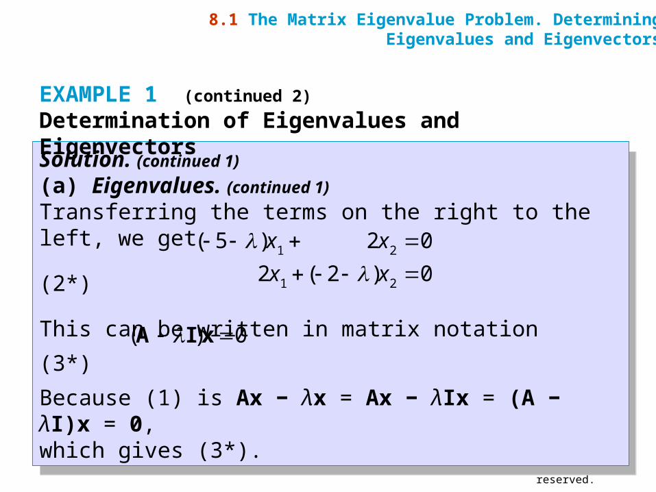
Transferring the terms on the right to the left, we get
(2*)
This can be written in matrix notation
(3*)
Because (1) is Ax − λx = Ax − λIx = (A − λI)x = 0, which gives (3*).
Solution. (continued 1)
(a) Eigenvalues. (continued 1)
Transferring the terms on the right to the left, we get
(2*)
This can be written in matrix notation
(3*)
Because (1) is Ax − λx = Ax − λIx = (A − λI)x = 0, which gives (3*).
8.1 The Matrix Eigenvalue Problem. DeterminingEigenvalues and Eigenvectors
EXAMPLE 1 (continued 2) Determination of Eigenvalues and Eigenvectors
1 2
1 2
( 5 ) 2 0
2 ( 2 ) 0
x x
x x
( ) 0 A I x
Advanced Engineering Mathematics, 10/e by Edwin KreyszigCopyright 2011 by John Wiley & Sons. All rights reserved.
Section 8.1 p9
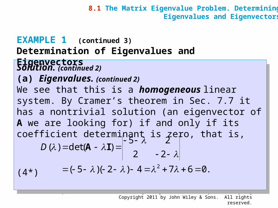
Solution. (continued 2)
(a) Eigenvalues. (continued 2)
We see that this is a homogeneous linear system. By Cramer’s theorem in Sec. 7.7 it has a nontrivial solution (an eigenvector of A we are looking for) if and only if its coefficient determinant is zero, that is,
(4*)
Solution. (continued 2)
(a) Eigenvalues. (continued 2)
We see that this is a homogeneous linear system. By Cramer’s theorem in Sec. 7.7 it has a nontrivial solution (an eigenvector of A we are looking for) if and only if its coefficient determinant is zero, that is,
(4*)
8.1 The Matrix Eigenvalue Problem. DeterminingEigenvalues and Eigenvectors
EXAMPLE 1 (continued 3) Determination of Eigenvalues and Eigenvectors
2
5 2( ) det( )
2 2
( 5 )( 2 ) 4 7 6 0.
D
A I
Advanced Engineering Mathematics, 10/e by Edwin KreyszigCopyright 2011 by John Wiley & Sons. All rights reserved.
Section 8.1 p10
Solution. (continued 3)
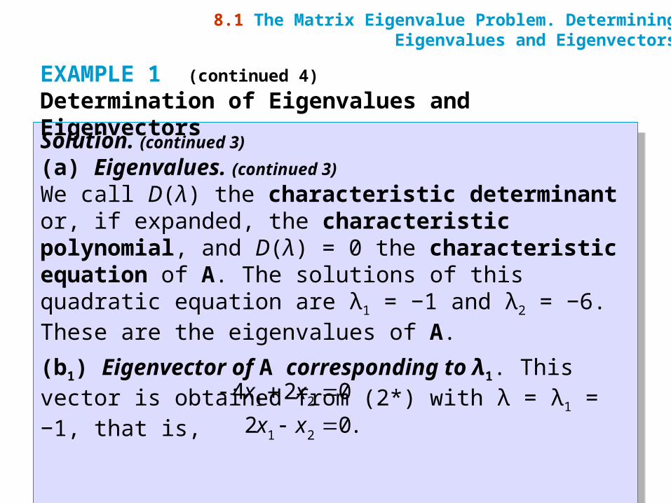
(a) Eigenvalues. (continued 3)
We call D(λ) the characteristic determinant or, if expanded, the characteristic polynomial, and D(λ) = 0 the characteristic equation of A. The solutions of this quadratic equation are λ1 = −1 and λ2 = −6. These are the eigenvalues of A.
(b1) Eigenvector of A corresponding to λ1. This vector is obtained from (2*) with λ = λ1 = −1, that is,
Solution. (continued 3)
(a) Eigenvalues. (continued 3)
We call D(λ) the characteristic determinant or, if expanded, the characteristic polynomial, and D(λ) = 0 the characteristic equation of A. The solutions of this quadratic equation are λ1 = −1 and λ2 = −6. These are the eigenvalues of A.
(b1) Eigenvector of A corresponding to λ1. This vector is obtained from (2*) with λ = λ1 = −1, that is,
8.1 The Matrix Eigenvalue Problem. DeterminingEigenvalues and Eigenvectors
EXAMPLE 1 (continued 4) Determination of Eigenvalues and Eigenvectors
1 2
1 2
4 2 0
2 0.
x x
x x
Advanced Engineering Mathematics, 10/e by Edwin KreyszigCopyright 2011 by John Wiley & Sons. All rights reserved.
Section 8.1 p11
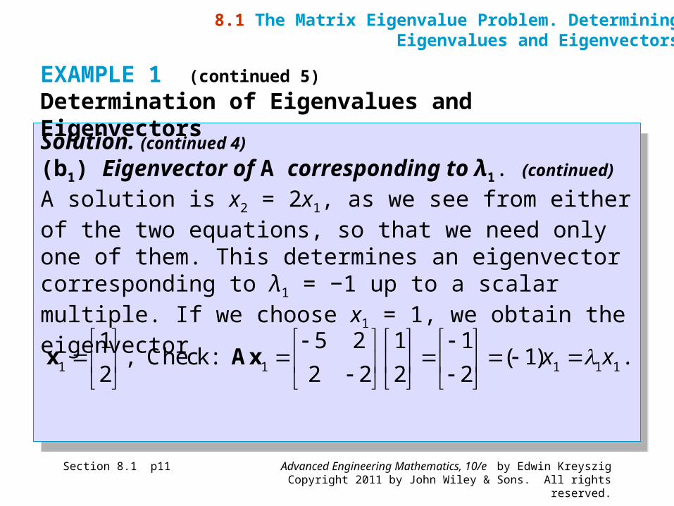
Solution. (continued 4)
(b1) Eigenvector of A corresponding to λ1. (continued)
A solution is x2 = 2x1, as we see from either of the two equations, so that we need only one of them. This determines an eigenvector corresponding to λ1 = −1 up to a scalar multiple. If we choose x1 = 1, we obtain the eigenvector
8.1 The Matrix Eigenvalue Problem. DeterminingEigenvalues and Eigenvectors
EXAMPLE 1 (continued 5) Determination of Eigenvalues and Eigenvectors
1 1 1 1 1
1 5 2 1 1, Check: ( 1) .
2 2 2 2 2x x
x Ax
Advanced Engineering Mathematics, 10/e by Edwin KreyszigCopyright 2011 by John Wiley & Sons. All rights reserved.
Section 8.1 p12
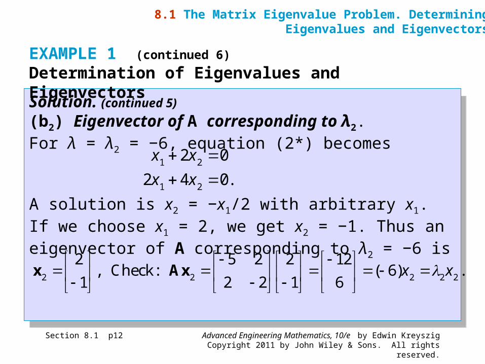
Solution. (continued 5)
(b2) Eigenvector of A corresponding to λ2. For λ = λ2 = −6, equation (2*) becomes
A solution is x2 = −x1/2 with arbitrary x1. If we choose x1 = 2, we get x2 = −1. Thus an eigenvector of A corresponding to λ2 = −6 is
Solution. (continued 5)
(b2) Eigenvector of A corresponding to λ2. For λ = λ2 = −6, equation (2*) becomes
A solution is x2 = −x1/2 with arbitrary x1. If we choose x1 = 2, we get x2 = −1. Thus an eigenvector of A corresponding to λ2 = −6 is
8.1 The Matrix Eigenvalue Problem. DeterminingEigenvalues and Eigenvectors
EXAMPLE 1 (continued 6) Determination of Eigenvalues and Eigenvectors
2 2 2 2 2
2 5 2 2 12, Check: ( 6) .
1 2 2 1 6x x
x Ax
1 2
1 2
2 0
2 4 0.
x x
x x
Advanced Engineering Mathematics, 10/e by Edwin KreyszigCopyright 2011 by John Wiley & Sons. All rights reserved.
Section 8.1 p13
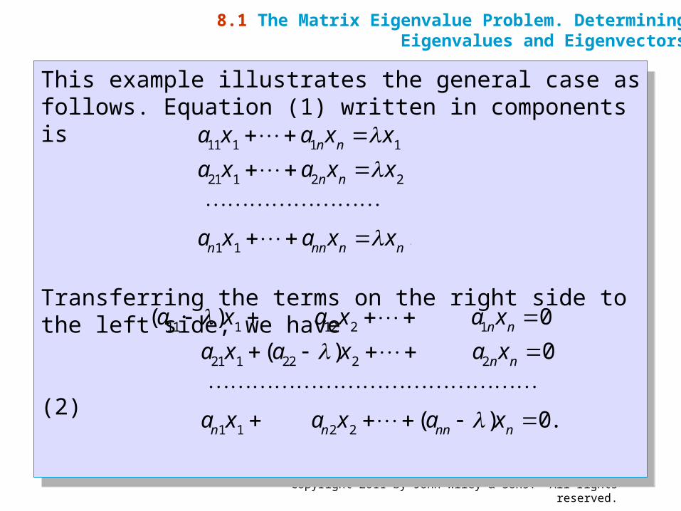
This example illustrates the general case as follows. Equation (1) written in components is
Transferring the terms on the right side to the left side, we have
(2)
This example illustrates the general case as follows. Equation (1) written in components is
Transferring the terms on the right side to the left side, we have
(2)
8.1 The Matrix Eigenvalue Problem. DeterminingEigenvalues and Eigenvectors
11 1 1 1
21 1 2 2
1 1
.
n n
n n
n nn n n
a x a x x
a x a x x
a x a x x
11 1 12 2 1
21 1 22 2 2
1 1 2 2
( ) 0
( ) 0
( ) 0.
n n
n n
n n nn n
a x a x a x
a x a x a x
a x a x a x
Advanced Engineering Mathematics, 10/e by Edwin KreyszigCopyright 2011 by John Wiley & Sons. All rights reserved.
Section 8.1 p14
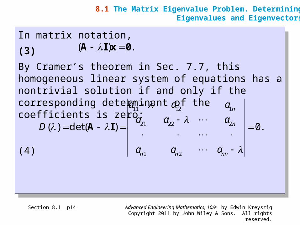
In matrix notation,
(3)
By Cramer’s theorem in Sec. 7.7, this homogeneous linear system of equations has a nontrivial solution if and only if the corresponding determinant of the coefficients is zero:
(4)
In matrix notation,
(3)
By Cramer’s theorem in Sec. 7.7, this homogeneous linear system of equations has a nontrivial solution if and only if the corresponding determinant of the coefficients is zero:
(4)
8.1 The Matrix Eigenvalue Problem. DeterminingEigenvalues and Eigenvectors
( ) . A I x 0
11 12 1
21 22 2
1 2
( ) det( ) 0.
n
n
n n nn
a a a
a a aD
a a a
A I
Advanced Engineering Mathematics, 10/e by Edwin KreyszigCopyright 2011 by John Wiley & Sons. All rights reserved.
Section 8.1 p15
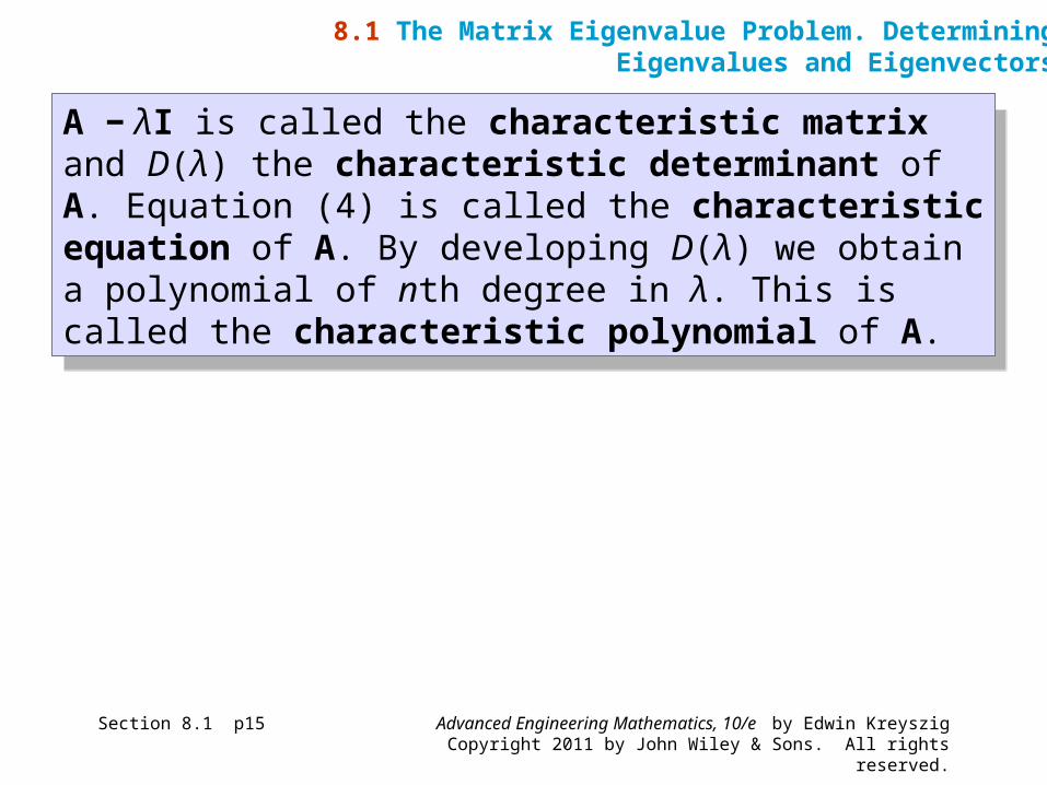
A − λI is called the characteristic matrix and D(λ) the characteristic determinant of A. Equation (4) is called the characteristic equation of A. By developing D(λ) we obtain a polynomial of nth degree in λ. This is called the characteristic polynomial of A.
A − λI is called the characteristic matrix and D(λ) the characteristic determinant of A. Equation (4) is called the characteristic equation of A. By developing D(λ) we obtain a polynomial of nth degree in λ. This is called the characteristic polynomial of A.
8.1 The Matrix Eigenvalue Problem. DeterminingEigenvalues and Eigenvectors
Advanced Engineering Mathematics, 10/e by Edwin KreyszigCopyright 2011 by John Wiley & Sons. All rights reserved.
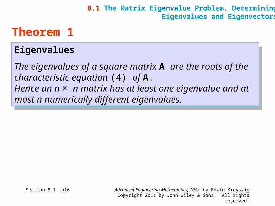
Eigenvalues
The eigenvalues of a square matrix A are the roots of the characteristic equation (4) of A.Hence an n × n matrix has at least one eigenvalue and at most n numerically different eigenvalues.
Eigenvalues
The eigenvalues of a square matrix A are the roots of the characteristic equation (4) of A.Hence an n × n matrix has at least one eigenvalue and at most n numerically different eigenvalues.
Section 8.1 p16
Theorem 1
8.1 The Matrix Eigenvalue Problem. DeterminingEigenvalues and Eigenvectors
Advanced Engineering Mathematics, 10/e by Edwin KreyszigCopyright 2011 by John Wiley & Sons. All rights reserved.
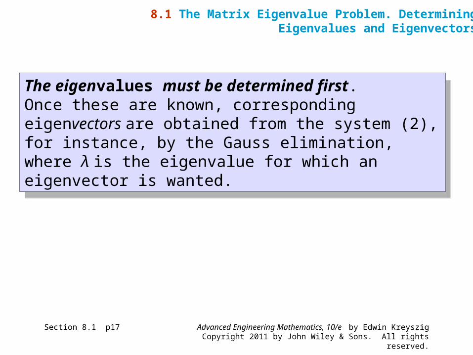
The eigenvalues must be determined first. Once these are known, corresponding eigenvectors are obtained from the system (2), for instance, by the Gauss elimination, where λ is the eigenvalue for which an eigenvector is wanted.
The eigenvalues must be determined first. Once these are known, corresponding eigenvectors are obtained from the system (2), for instance, by the Gauss elimination, where λ is the eigenvalue for which an eigenvector is wanted.
Section 8.1 p17
8.1 The Matrix Eigenvalue Problem. DeterminingEigenvalues and Eigenvectors
Advanced Engineering Mathematics, 10/e by Edwin KreyszigCopyright 2011 by John Wiley & Sons. All rights reserved.
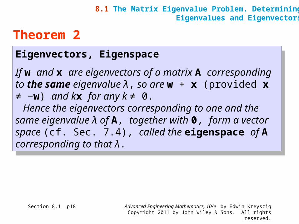
Eigenvectors, Eigenspace
If w and x are eigenvectors of a matrix A corresponding to the same eigenvalue λ, so are w + x (provided x ≠ −w) and kx for any k ≠ 0.
Hence the eigenvectors corresponding to one and the same eigenvalue λ of A, together with 0, form a vector space (cf. Sec. 7.4), called the eigenspace of A corresponding to that λ.
Section 8.1 p18
Theorem 2
8.1 The Matrix Eigenvalue Problem. DeterminingEigenvalues and Eigenvectors
Advanced Engineering Mathematics, 10/e by Edwin KreyszigCopyright 2011 by John Wiley & Sons. All rights reserved.
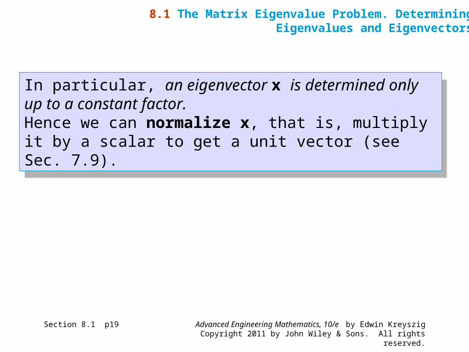
In particular, an eigenvector x is determined only up to a constant factor. Hence we can normalize x, that is, multiply it by a scalar to get a unit vector (see Sec. 7.9).
In particular, an eigenvector x is determined only up to a constant factor. Hence we can normalize x, that is, multiply it by a scalar to get a unit vector (see Sec. 7.9).
Section 8.1 p19
8.1 The Matrix Eigenvalue Problem. DeterminingEigenvalues and Eigenvectors
Advanced Engineering Mathematics, 10/e by Edwin KreyszigCopyright 2011 by John Wiley & Sons. All rights reserved.
Section 8.1 p20
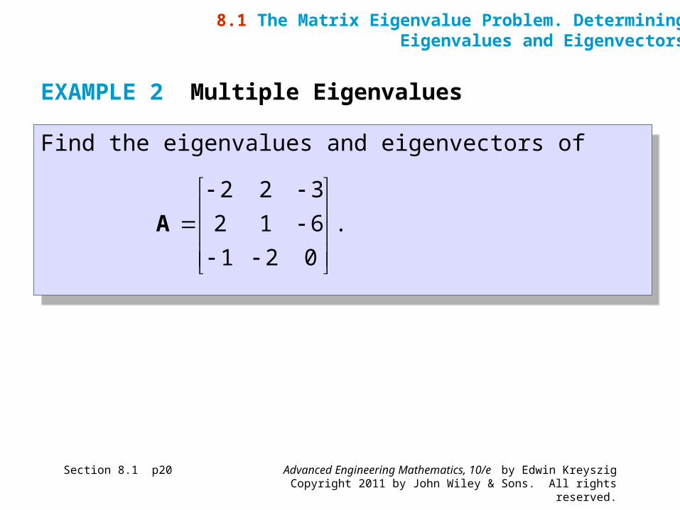
Find the eigenvalues and eigenvectors ofFind the eigenvalues and eigenvectors of
8.1 The Matrix Eigenvalue Problem. DeterminingEigenvalues and Eigenvectors
EXAMPLE 2 Multiple Eigenvalues
2 2 3
2 1 6 .
1 2 0
A
Advanced Engineering Mathematics, 10/e by Edwin KreyszigCopyright 2011 by John Wiley & Sons. All rights reserved.
Section 8.1 p21
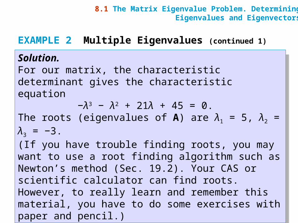
Solution. For our matrix, the characteristic determinant gives the characteristic equation
−λ3 − λ2 + 21λ + 45 = 0. The roots (eigenvalues of A) are λ1 = 5, λ2 = λ3 = −3. (If you have trouble finding roots, you may want to use a root finding algorithm such as Newton’s method (Sec. 19.2). Your CAS or scientific calculator can find roots. However, to really learn and remember this material, you have to do some exercises with paper and pencil.)
8.1 The Matrix Eigenvalue Problem. DeterminingEigenvalues and Eigenvectors
EXAMPLE 2 Multiple Eigenvalues (continued 1)
Advanced Engineering Mathematics, 10/e by Edwin KreyszigCopyright 2011 by John Wiley & Sons. All rights reserved.
Section 8.1 p22
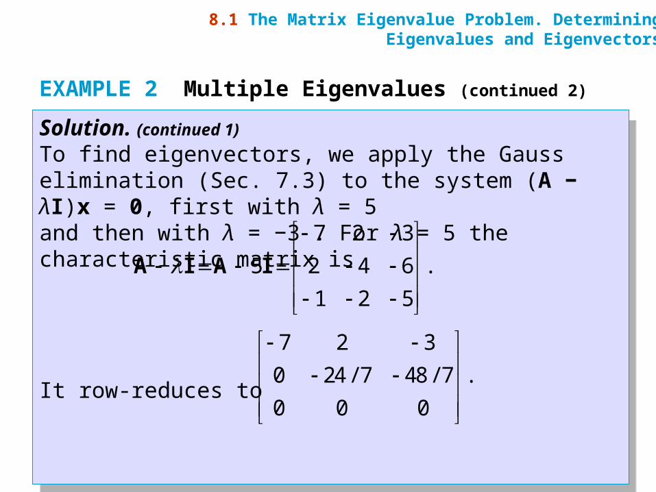
Solution. (continued 1)
To find eigenvectors, we apply the Gauss elimination (Sec. 7.3) to the system (A − λI)x = 0, first with λ = 5and then with λ = −3 . For λ = 5 the characteristic matrix is
It row-reduces to
Solution. (continued 1)
To find eigenvectors, we apply the Gauss elimination (Sec. 7.3) to the system (A − λI)x = 0, first with λ = 5and then with λ = −3 . For λ = 5 the characteristic matrix is
It row-reduces to
8.1 The Matrix Eigenvalue Problem. DeterminingEigenvalues and Eigenvectors
EXAMPLE 2 Multiple Eigenvalues (continued 2)
7 2 3
5 2 4 6 .
1 2 5
A I A I
7 2 3
0 24/ 7 48/ 7 .
0 0 0
Advanced Engineering Mathematics, 10/e by Edwin KreyszigCopyright 2011 by John Wiley & Sons. All rights reserved.
Section 8.1 p23
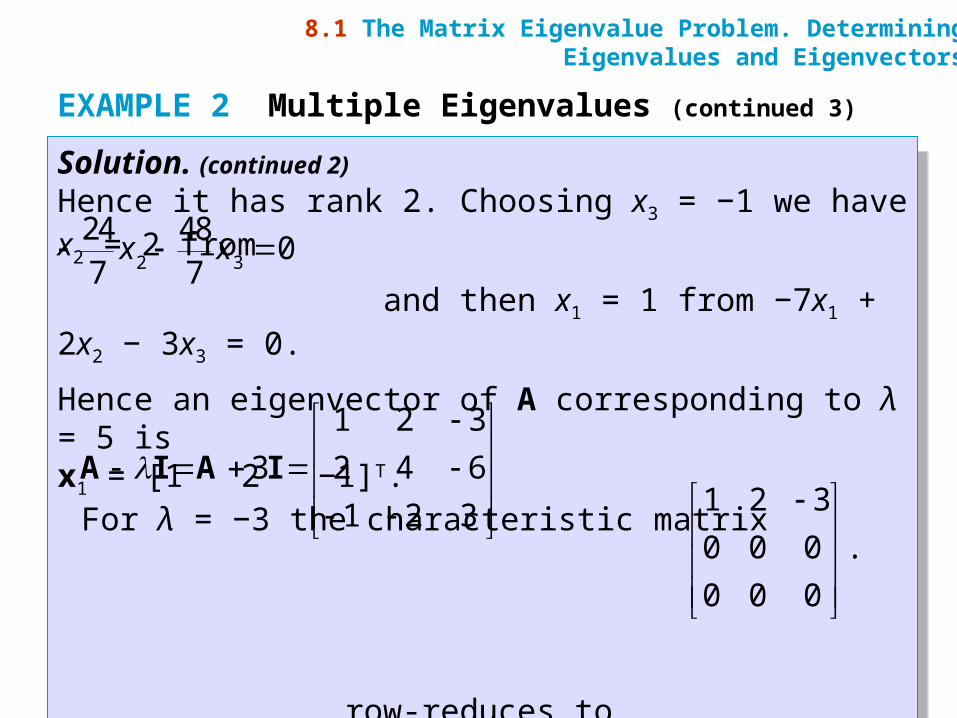
Solution. (continued 2)
Hence it has rank 2. Choosing x3 = −1 we have x2 = 2 from
and then x1 = 1 from −7x1 + 2x2 − 3x3 = 0.
Hence an eigenvector of A corresponding to λ = 5 is x1 = [1 2 −1]T.
For λ = −3 the characteristic matrix
row-reduces to
Solution. (continued 2)
Hence it has rank 2. Choosing x3 = −1 we have x2 = 2 from
and then x1 = 1 from −7x1 + 2x2 − 3x3 = 0.
Hence an eigenvector of A corresponding to λ = 5 is x1 = [1 2 −1]T.
For λ = −3 the characteristic matrix
row-reduces to
8.1 The Matrix Eigenvalue Problem. DeterminingEigenvalues and Eigenvectors
EXAMPLE 2 Multiple Eigenvalues (continued 3)
1 2 3
3 2 4 6
1 2 3
A I A I1 2 3
0 0 0 .
0 0 0
2 3
24 480
7 7x x
Advanced Engineering Mathematics, 10/e by Edwin KreyszigCopyright 2011 by John Wiley & Sons. All rights reserved.
Section 8.1 p24
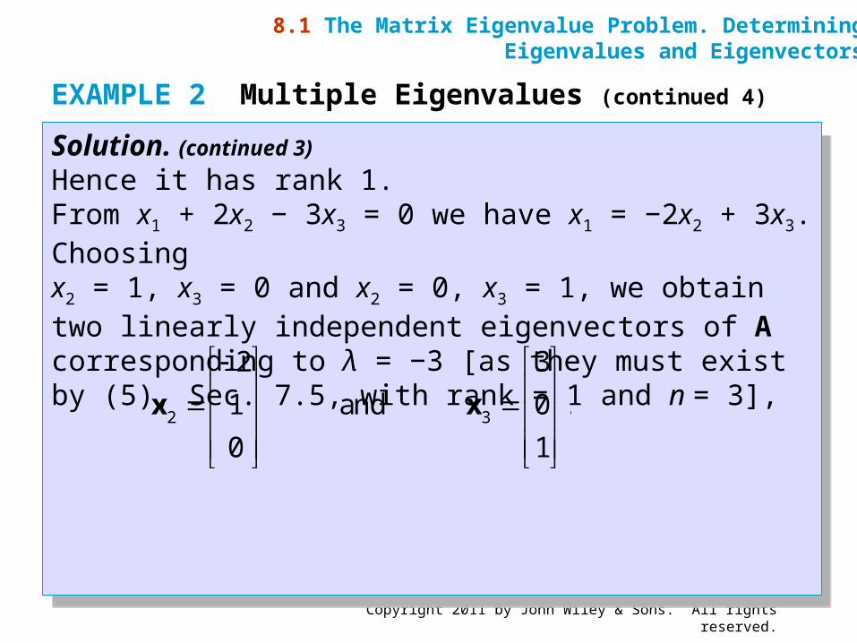
Solution. (continued 3)
Hence it has rank 1. From x1 + 2x2 − 3x3 = 0 we have x1 = −2x2 + 3x3. Choosing x2 = 1, x3 = 0 and x2 = 0, x3 = 1, we obtain two linearly independent eigenvectors of A corresponding to λ = −3 [as they must exist by (5), Sec. 7.5, with rank = 1 and n = 3],
Solution. (continued 3)
Hence it has rank 1. From x1 + 2x2 − 3x3 = 0 we have x1 = −2x2 + 3x3. Choosing x2 = 1, x3 = 0 and x2 = 0, x3 = 1, we obtain two linearly independent eigenvectors of A corresponding to λ = −3 [as they must exist by (5), Sec. 7.5, with rank = 1 and n = 3],
8.1 The Matrix Eigenvalue Problem. DeterminingEigenvalues and Eigenvectors
EXAMPLE 2 Multiple Eigenvalues (continued 4)
2 3
2 3
1 and 0 .
0 1
x x

Advanced Engineering Mathematics, 10/e by Edwin KreyszigCopyright 2011 by John Wiley & Sons. All rights reserved.
Section 8.1 p25
The order Mλ of an eigenvalue λ as a root of the characteristic polynomial is called the algebraic multiplicity of λ. The number mλ of linearly independent eigenvectors corresponding to λ is called the geometric multiplicity of λ. Thus mλ is the dimension of the eigenspace corresponding to this λ.
Since the characteristic polynomial has degree n, the sum of all the algebraic multiplicities must equal n. In Example 2 for λ = −3 we have mλ = Mλ = 2. In general, mλ ≤ Mλ, as can be shown. The difference Δλ = Mλ − mλ is called the defect of λ. Thus Δ−3 = 0 in Example 2, but positive defects Δλ can easily occur.
8.1 The Matrix Eigenvalue Problem. DeterminingEigenvalues and Eigenvectors
Advanced Engineering Mathematics, 10/e by Edwin KreyszigCopyright 2011 by John Wiley & Sons. All rights reserved.
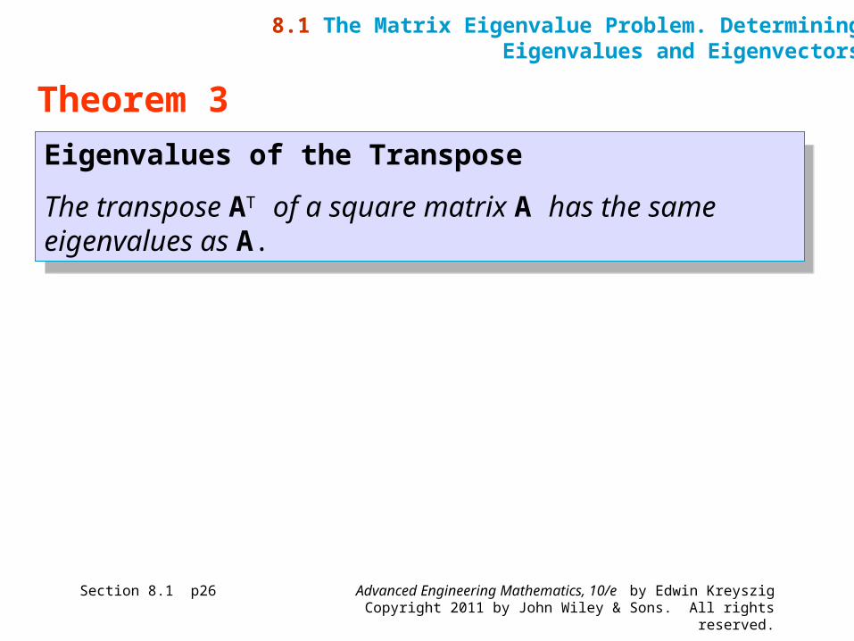
Eigenvalues of the Transpose
The transpose AT of a square matrix A has the same eigenvalues as A.
Eigenvalues of the Transpose
The transpose AT of a square matrix A has the same eigenvalues as A.
Section 8.1 p26
Theorem 3
8.1 The Matrix Eigenvalue Problem. DeterminingEigenvalues and Eigenvectors
Advanced Engineering Mathematics, 10/e by Edwin KreyszigCopyright 2011 by John Wiley & Sons. All rights reserved.
Section 8.2 p27
8.2 Some Applications of Eigenvalue Problems
8.2 Some Applications of Eigenvalue Problems
Advanced Engineering Mathematics, 10/e by Edwin KreyszigCopyright 2011 by John Wiley & Sons. All rights reserved.
Section 8.2 p28
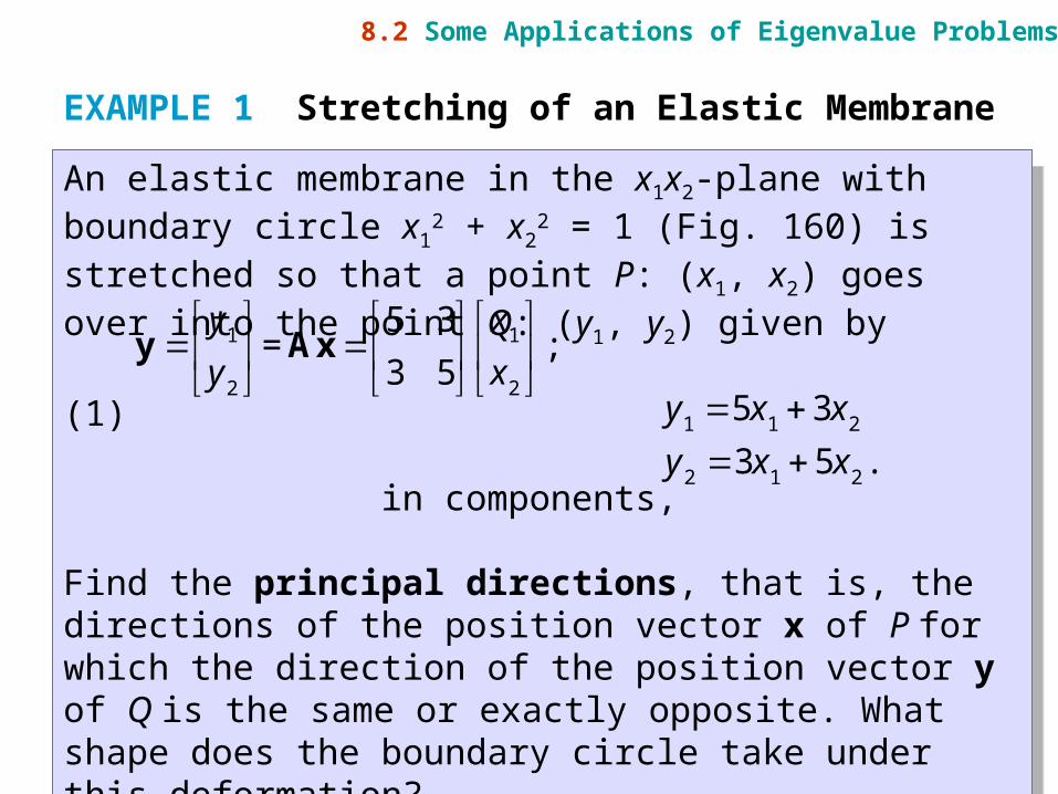
An elastic membrane in the x1x2-plane with boundary circle x1
2 + x22 = 1 (Fig. 160) is stretched so that a
point P: (x1, x2) goes over into the point Q: (y1, y2) given by
(1)
in components,
Find the principal directions, that is, the directions of the position vector x of P for which the direction of the position vector y of Q is the same or exactly opposite. What shape does the boundary circle take under this deformation?
EXAMPLE 1 Stretching of an Elastic Membrane
8.2 Some Applications of Eigenvalue Problems
1 1
2 2
5 3= ;
3 5
y x
y x
y Ax
1 1 2
2 1 2
5 3
3 5 .
y x x
y x x
Advanced Engineering Mathematics, 10/e by Edwin KreyszigCopyright 2011 by John Wiley & Sons. All rights reserved.
Section 8.2 p29
Solution. We are looking for vectors x such that y = λx. Since y = Ax, this gives Ax = λx, the equation of an eigenvalue problem. In components, Ax = λx is
(2) or
The characteristic equation is
(3)
Solution. We are looking for vectors x such that y = λx. Since y = Ax, this gives Ax = λx, the equation of an eigenvalue problem. In components, Ax = λx is
(2) or
The characteristic equation is
(3)
EXAMPLE 1 (continued 1) Stretching of an Elastic Membrane
8.2 Some Applications of Eigenvalue Problems
1 2 1
1 2 2
5 3
3 5
x x x
x x x
1 2
1 2
(5 ) 3 0
3 (5 ) 0.
x x
x x
25 3(5 ) 9 0.
3 5
Advanced Engineering Mathematics, 10/e by Edwin KreyszigCopyright 2011 by John Wiley & Sons. All rights reserved.
Section 8.2 p30
Solution. (continued 1)
Its solutions are λ1 = 8 and λ2 = 2. These are the eigenvalues of our problem. For λ1 = λ2 = 8, our system (2)becomes
−3x1 + 3x2 = 0, Solution x2 = x1, x1 arbitrary,
3x1 − 3x2 = 0. for instance, x1 = x2 = 1.
For λ2 = 2, our system (2) becomes
3x1 + 3x2 = 0, Solution x2 = −x1, x1 arbitrary,
3x1 + 3x2 = 0. for instance, x1 = 1, x2 = −1.
EXAMPLE 1 (continued 2) Stretching of an Elastic Membrane
8.2 Some Applications of Eigenvalue Problems
Advanced Engineering Mathematics, 10/e by Edwin KreyszigCopyright 2011 by John Wiley & Sons. All rights reserved.
Section 8.2 p31
Solution. (continued 2)
We thus obtain as eigenvectors of A, for instance, [1 1]T corresponding to λ1 and [1 −1]T corresponding to λ2 (or a nonzero scalar multiple of these). These vectors make 45° and 135° angles with the positive x1-direction. They give the principal directions, the answer to our problem.
The eigenvalues show that in the principal directions the membrane is stretched by factors 8 and 2, respectively; see Fig. 160.
EXAMPLE 1 (continued 3) Stretching of an Elastic Membrane
8.2 Some Applications of Eigenvalue Problems
Advanced Engineering Mathematics, 10/e by Edwin KreyszigCopyright 2011 by John Wiley & Sons. All rights reserved.
Section 8.2 p32
Solution. (continued 3)
Accordingly, if we choose the principal directions as directions of a new Cartesian u1u2 coordinate system,say, with the positive u1-semi-axis in the first quadrant and the positive u2-semi-axis in the second quadrant ofthe x1x2-system, and if we set u1 = r cos φ, u2 = r sin φ, then a boundary point of the unstretched circularmembrane has coordinates cos φ, sin φ. Hence, after the stretch we have
z1 = 8 cos φ , z2 = 2 sin φ .
EXAMPLE 1 (continued 4) Stretching of an Elastic Membrane
8.2 Some Applications of Eigenvalue Problems
Advanced Engineering Mathematics, 10/e by Edwin KreyszigCopyright 2011 by John Wiley & Sons. All rights reserved.
Section 8.2 p33
Solution. (continued 4)
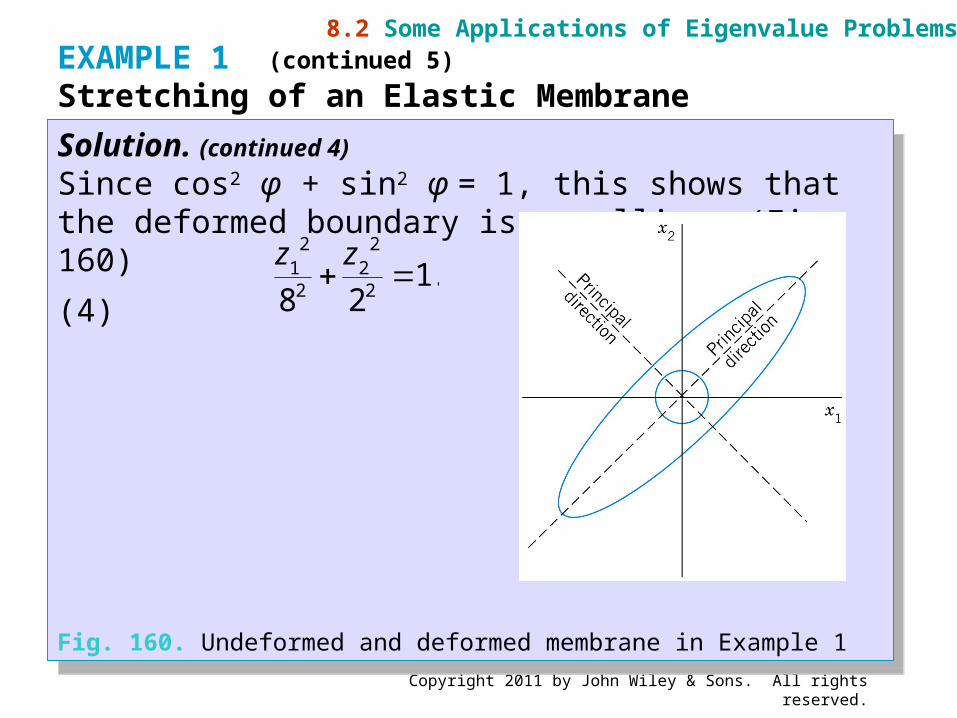
Since cos2 φ + sin2 φ = 1, this shows that the deformed boundary is an ellipse (Fig. 160)
(4)
Fig. 160. Undeformed and deformed membrane in Example 1
Solution. (continued 4)
Since cos2 φ + sin2 φ = 1, this shows that the deformed boundary is an ellipse (Fig. 160)
(4)
Fig. 160. Undeformed and deformed membrane in Example 1
EXAMPLE 1 (continued 5) Stretching of an Elastic Membrane
8.2 Some Applications of Eigenvalue Problems
2 21 22 2
1.8 2
z z
Advanced Engineering Mathematics, 10/e by Edwin KreyszigCopyright 2011 by John Wiley & Sons. All rights reserved.
Section 8.3 p34
8.3 Symmetric, Skew-Symmetric,and Orthogonal Matrices
8.3 Symmetric, Skew-Symmetric,and Orthogonal Matrices
Advanced Engineering Mathematics, 10/e by Edwin KreyszigCopyright 2011 by John Wiley & Sons. All rights reserved.
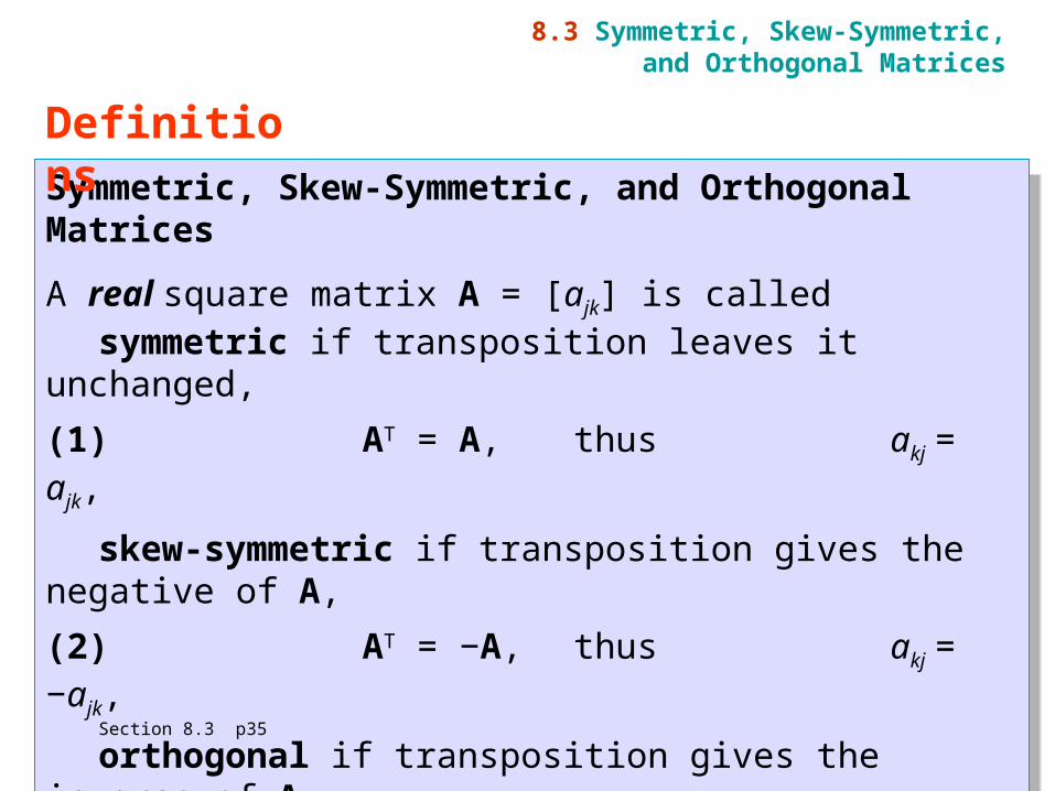
Symmetric, Skew-Symmetric, and Orthogonal Matrices
A real square matrix A = [ajk] is calledsymmetric if transposition leaves it unchanged,
(1) AT = A, thus akj = ajk,
skew-symmetric if transposition gives the negative of A,
(2) AT = −A, thus akj = −ajk,
orthogonal if transposition gives the inverse of A,
(3) AT = A−1.
Section 8.3 p35
Definitions
8.3 Symmetric, Skew-Symmetric,and Orthogonal Matrices
Advanced Engineering Mathematics, 10/e by Edwin KreyszigCopyright 2011 by John Wiley & Sons. All rights reserved.
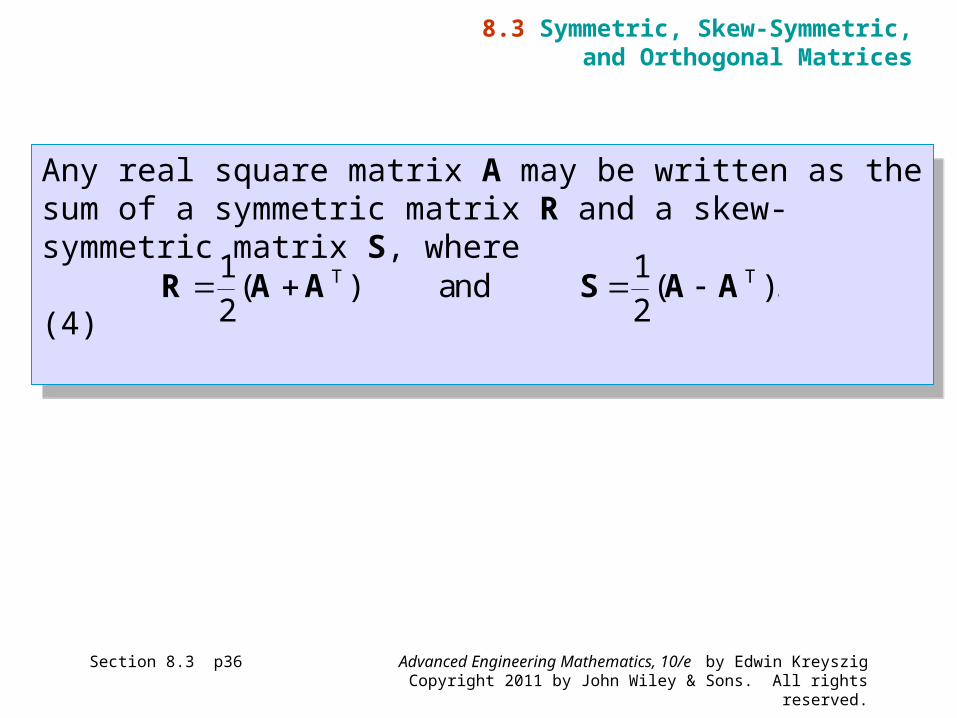
Any real square matrix A may be written as the sum of a symmetric matrix R and a skew-symmetric matrix S, where
(4)
Any real square matrix A may be written as the sum of a symmetric matrix R and a skew-symmetric matrix S, where
(4)
Section 8.3 p36
8.3 Symmetric, Skew-Symmetric,and Orthogonal Matrices
1 1( ) and ( ).
2 2 R A A S A AT T
Advanced Engineering Mathematics, 10/e by Edwin KreyszigCopyright 2011 by John Wiley & Sons. All rights reserved.
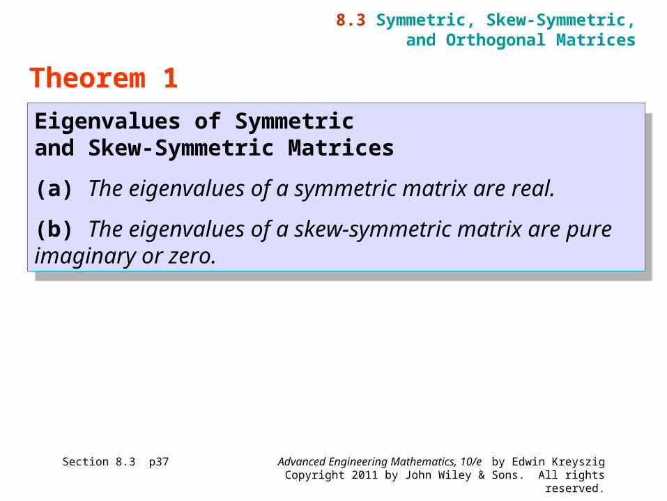
Eigenvalues of Symmetric and Skew-Symmetric Matrices
(a) The eigenvalues of a symmetric matrix are real.
(b) The eigenvalues of a skew-symmetric matrix are pure imaginary or zero.
Eigenvalues of Symmetric and Skew-Symmetric Matrices
(a) The eigenvalues of a symmetric matrix are real.
(b) The eigenvalues of a skew-symmetric matrix are pure imaginary or zero.
Section 8.3 p37
Theorem 1
8.3 Symmetric, Skew-Symmetric,and Orthogonal Matrices
Advanced Engineering Mathematics, 10/e by Edwin KreyszigCopyright 2011 by John Wiley & Sons. All rights reserved.
Section 8.3 p38
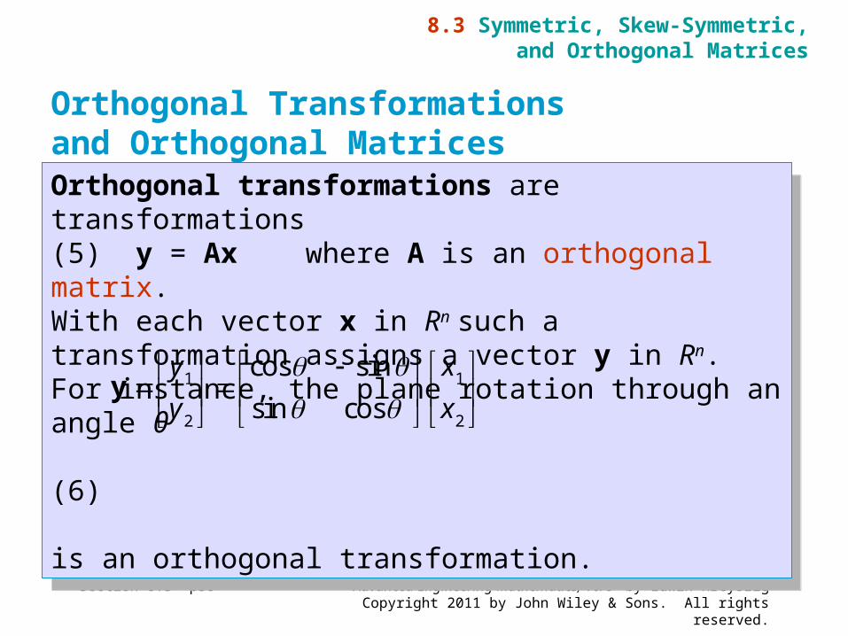
Orthogonal transformations are transformations(5) y = Ax where A is an orthogonal matrix.With each vector x in Rn such a transformation assigns a vector y in Rn. For instance, the plane rotation through an angle θ
(6)
is an orthogonal transformation.
Orthogonal transformations are transformations(5) y = Ax where A is an orthogonal matrix.With each vector x in Rn such a transformation assigns a vector y in Rn. For instance, the plane rotation through an angle θ
(6)
is an orthogonal transformation.
Orthogonal Transformations and Orthogonal Matrices
8.3 Symmetric, Skew-Symmetric,and Orthogonal Matrices
1 1
2 2
cos sin
sin cos
y x
y x
y
Advanced Engineering Mathematics, 10/e by Edwin KreyszigCopyright 2011 by John Wiley & Sons. All rights reserved.
Section 8.3 p39
It can be shown that any orthogonal transformation in the plane or in three-dimensional space is a rotation (possibly combined with a reflection in a straight line or a plane, respectively).
The main reason for the importance of orthogonal matrices is as follows.
It can be shown that any orthogonal transformation in the plane or in three-dimensional space is a rotation (possibly combined with a reflection in a straight line or a plane, respectively).
The main reason for the importance of orthogonal matrices is as follows.
Orthogonal Transformations and Orthogonal Matrices (continued)
8.3 Symmetric, Skew-Symmetric,and Orthogonal Matrices

Advanced Engineering Mathematics, 10/e by Edwin KreyszigCopyright 2011 by John Wiley & Sons. All rights reserved.
Invariance of Inner Product
An orthogonal transformation preserves the value of the inner product of vectors a and b in Rn, defined by
(7)
That is, for any a and b in Rn, orthogonal n × n matrix A, and u = Aa, v = Ab we have u · v = a · b.Hence the transformation also preserves the length or norm of any vector a in Rn given by(8)
Invariance of Inner Product
An orthogonal transformation preserves the value of the inner product of vectors a and b in Rn, defined by
(7)
That is, for any a and b in Rn, orthogonal n × n matrix A, and u = Aa, v = Ab we have u · v = a · b.Hence the transformation also preserves the length or norm of any vector a in Rn given by(8)Section 8.3 p40
Theorem 2
8.3 Symmetric, Skew-Symmetric,and Orthogonal Matrices
1
1 .n
n
b
a a
b
a b a b T
. a a a a a T
Advanced Engineering Mathematics, 10/e by Edwin KreyszigCopyright 2011 by John Wiley & Sons. All rights reserved.
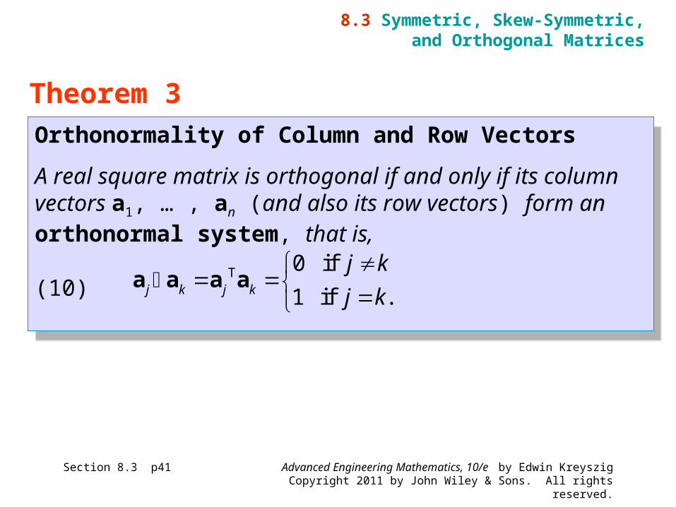
Orthonormality of Column and Row Vectors
A real square matrix is orthogonal if and only if its column vectors a1, … , an (and also its row vectors) form an orthonormal system, that is,
(10)
Orthonormality of Column and Row Vectors
A real square matrix is orthogonal if and only if its column vectors a1, … , an (and also its row vectors) form an orthonormal system, that is,
(10)
Section 8.3 p41
Theorem 3
8.3 Symmetric, Skew-Symmetric,and Orthogonal Matrices
0 if
1 if .j k j k
j k
j k
a a a a T
Advanced Engineering Mathematics, 10/e by Edwin KreyszigCopyright 2011 by John Wiley & Sons. All rights reserved.
Determinant of an Orthogonal Matrix
The determinant of an orthogonal matrix has the value +1 or −1.
Determinant of an Orthogonal Matrix
The determinant of an orthogonal matrix has the value +1 or −1.
Section 8.3 p42
Theorem 4
8.3 Symmetric, Skew-Symmetric,and Orthogonal Matrices
Advanced Engineering Mathematics, 10/e by Edwin KreyszigCopyright 2011 by John Wiley & Sons. All rights reserved.
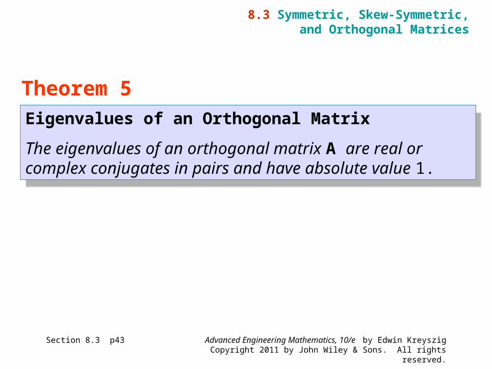
Eigenvalues of an Orthogonal Matrix
The eigenvalues of an orthogonal matrix A are real or complex conjugates in pairs and have absolute value 1.
Eigenvalues of an Orthogonal Matrix
The eigenvalues of an orthogonal matrix A are real or complex conjugates in pairs and have absolute value 1.
Section 8.3 p43
Theorem 5
8.3 Symmetric, Skew-Symmetric,and Orthogonal Matrices
Advanced Engineering Mathematics, 10/e by Edwin KreyszigCopyright 2011 by John Wiley & Sons. All rights reserved.
Section 8.4 p44
8.4 Eigenbases. Diagonalization.Quadratic Forms
8.4 Eigenbases. Diagonalization.Quadratic Forms
Advanced Engineering Mathematics, 10/e by Edwin KreyszigCopyright 2011 by John Wiley & Sons. All rights reserved.
Section 8.4 p45
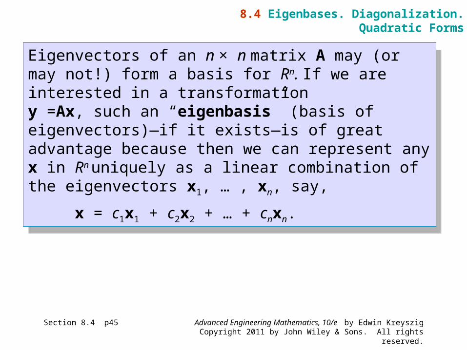
Eigenvectors of an n × n matrix A may (or may not!) form a basis for Rn. If we are interested in a transformation y =Ax, such an “eigenbasis” (basis of eigenvectors)—if it exists—is of great advantage because then we can represent any x in Rn
uniquely as a linear combination of the eigenvectors x1, … , xn, say,
x = c1x1 + c2x2 + … + cnxn.
8.4 Eigenbases. Diagonalization.Quadratic Forms
Advanced Engineering Mathematics, 10/e by Edwin KreyszigCopyright 2011 by John Wiley & Sons. All rights reserved.
Section 8.4 p46
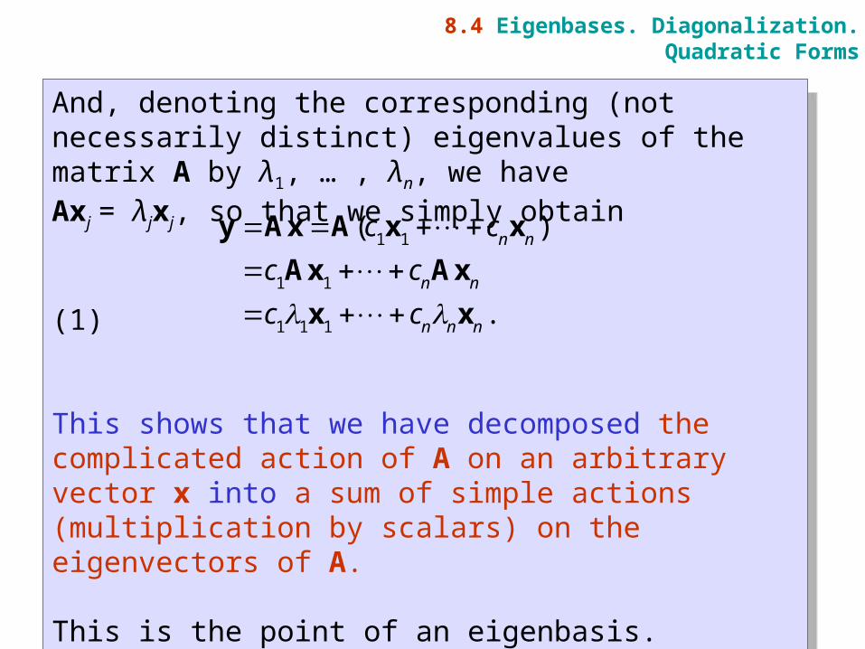
And, denoting the corresponding (not necessarily distinct) eigenvalues of the matrix A by λ1, … , λn, we have Axj = λjxj, so that we simply obtain
(1)
This shows that we have decomposed the complicated action of A on an arbitrary vector x into a sum of simple actions (multiplication by scalars) on the eigenvectors of A.
This is the point of an eigenbasis.
8.4 Eigenbases. Diagonalization.Quadratic Forms
1 1
1 1
1 1 1
( )
.
n n
n n
n n n
c c
c c
c c
y Ax A x x
Ax Ax
x x
Advanced Engineering Mathematics, 10/e by Edwin KreyszigCopyright 2011 by John Wiley & Sons. All rights reserved.
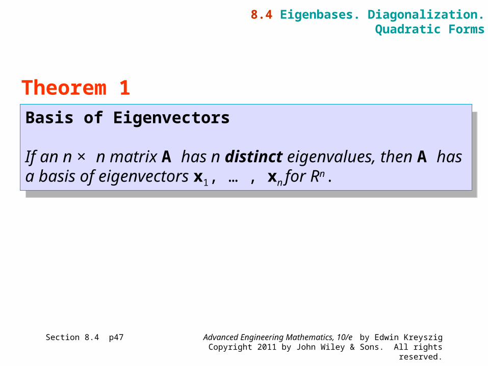
Basis of Eigenvectors
If an n × n matrix A has n distinct eigenvalues, then A has a basis of eigenvectors x1, … , xn for Rn.
Basis of Eigenvectors
If an n × n matrix A has n distinct eigenvalues, then A has a basis of eigenvectors x1, … , xn for Rn.
Section 8.4 p47
Theorem 1
8.4 Eigenbases. Diagonalization.Quadratic Forms
Advanced Engineering Mathematics, 10/e by Edwin KreyszigCopyright 2011 by John Wiley & Sons. All rights reserved.
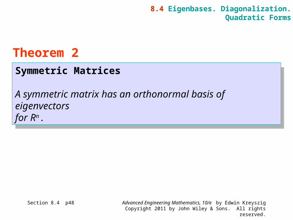
Symmetric Matrices
A symmetric matrix has an orthonormal basis of eigenvectors for Rn.
Symmetric Matrices
A symmetric matrix has an orthonormal basis of eigenvectors for Rn.
Section 8.4 p48
Theorem 2
8.4 Eigenbases. Diagonalization.Quadratic Forms
Advanced Engineering Mathematics, 10/e by Edwin KreyszigCopyright 2011 by John Wiley & Sons. All rights reserved.
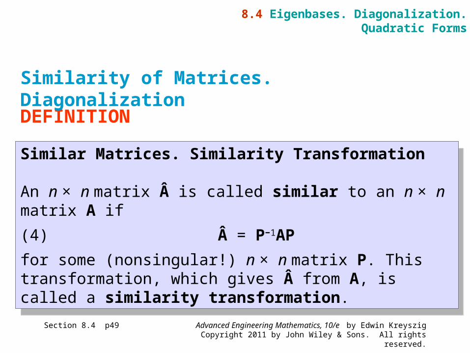
Similar Matrices. Similarity Transformation
An n × n matrix  is called similar to an n × n matrix A if
(4) Â = P−1AP
for some (nonsingular!) n × n matrix P. This transformation, which gives  from A, is called a similarity transformation.
Similar Matrices. Similarity Transformation
An n × n matrix  is called similar to an n × n matrix A if
(4) Â = P−1AP
for some (nonsingular!) n × n matrix P. This transformation, which gives  from A, is called a similarity transformation.
Section 8.4 p49
DEFINITION
Similarity of Matrices. Diagonalization
8.4 Eigenbases. Diagonalization.Quadratic Forms
Advanced Engineering Mathematics, 10/e by Edwin KreyszigCopyright 2011 by John Wiley & Sons. All rights reserved.
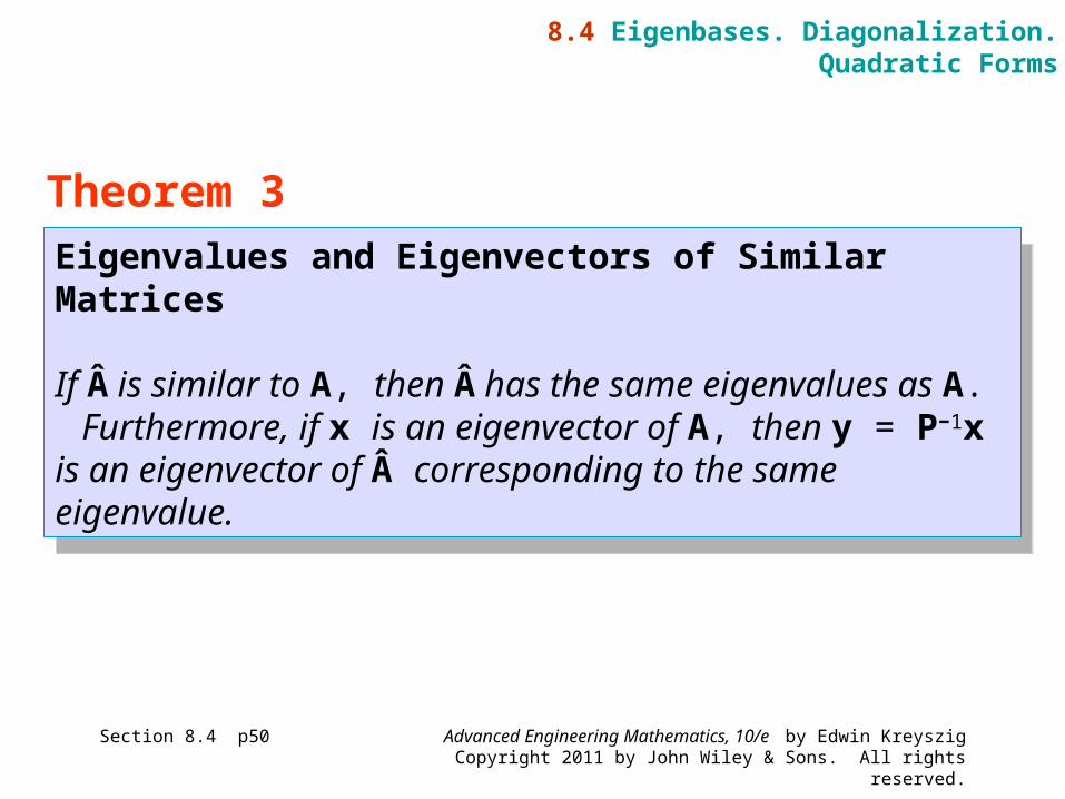
Eigenvalues and Eigenvectors of Similar Matrices
If  is similar to A, then  has the same eigenvalues as A.
Furthermore, if x is an eigenvector of A, then y = P−1x is an eigenvector of  corresponding to the same eigenvalue.
Eigenvalues and Eigenvectors of Similar Matrices
If  is similar to A, then  has the same eigenvalues as A.
Furthermore, if x is an eigenvector of A, then y = P−1x is an eigenvector of  corresponding to the same eigenvalue.
Section 8.4 p50
Theorem 3
8.4 Eigenbases. Diagonalization.Quadratic Forms
Advanced Engineering Mathematics, 10/e by Edwin KreyszigCopyright 2011 by John Wiley & Sons. All rights reserved.
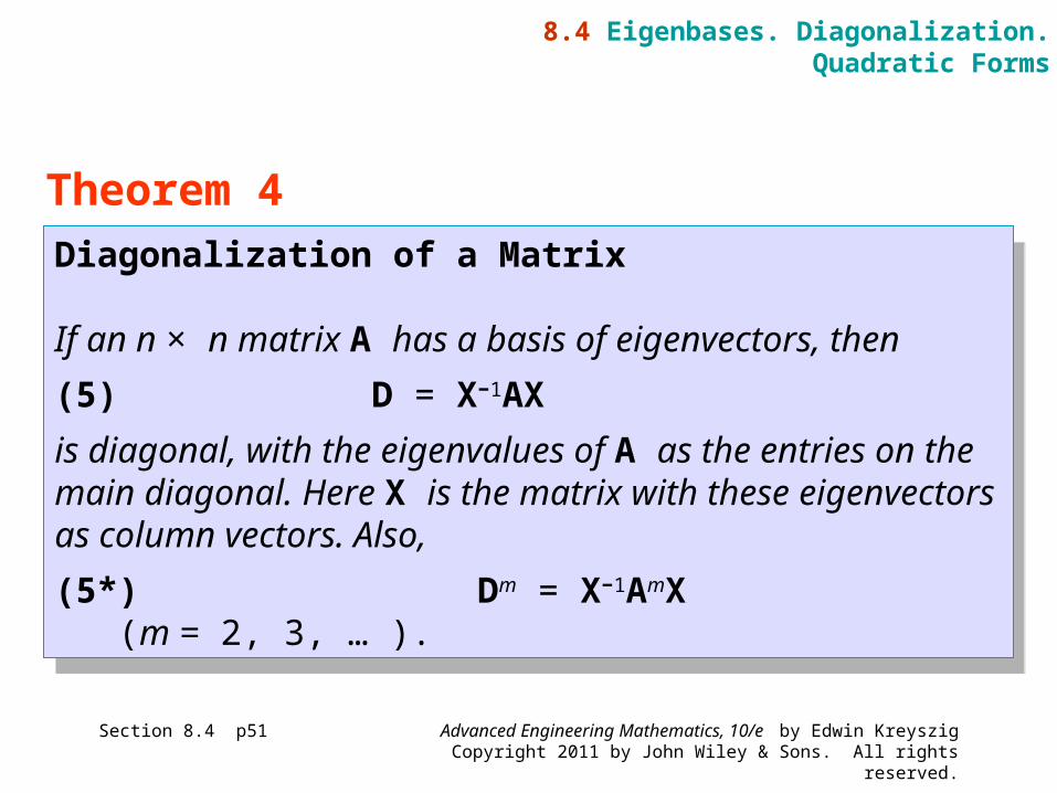
Diagonalization of a Matrix
If an n × n matrix A has a basis of eigenvectors, then
(5) D = X−1AX
is diagonal, with the eigenvalues of A as the entries on the main diagonal. Here X is the matrix with these eigenvectors as column vectors. Also,
(5*) Dm = X−1AmX (m = 2, 3, … ).
Diagonalization of a Matrix
If an n × n matrix A has a basis of eigenvectors, then
(5) D = X−1AX
is diagonal, with the eigenvalues of A as the entries on the main diagonal. Here X is the matrix with these eigenvectors as column vectors. Also,
(5*) Dm = X−1AmX (m = 2, 3, … ).
Section 8.4 p51
Theorem 4
8.4 Eigenbases. Diagonalization.Quadratic Forms

Advanced Engineering Mathematics, 10/e by Edwin KreyszigCopyright 2011 by John Wiley & Sons. All rights reserved.
Section 8.4 p52
Diagonalize
Solution. The characteristic determinant gives the characteristic equation −λ3 −λ2 + 12λ = 0. The roots (eigenvalues of A) are λ1 = 3, λ2 = −4, λ3 = 0. By the Gauss elimination applied to (A − λI)x = 0 with λ = λ1, λ2, λ3 we find eigenvectors and then X−1 by the Gauss–Jordan elimination (Sec. 7.8, Example 1).
EXAMPLE 4 Diagonalization
8.4 Eigenbases. Diagonalization.Quadratic Forms
7.3 0.2 3.7
11.5 1.0 5.5 .
17.7 1.8 9.3
A
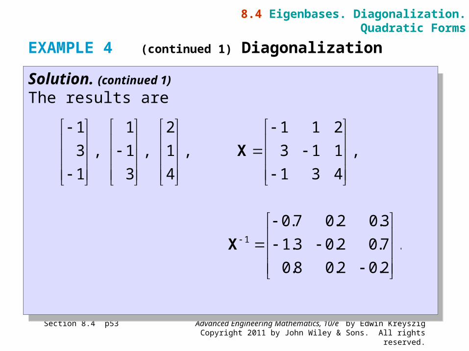
Advanced Engineering Mathematics, 10/e by Edwin KreyszigCopyright 2011 by John Wiley & Sons. All rights reserved.
Section 8.4 p53
Solution. (continued 1)
The results are
Solution. (continued 1)
The results are
EXAMPLE 4 (continued 1) Diagonalization
8.4 Eigenbases. Diagonalization.Quadratic Forms
1 1 2
3 1 1 ,
1 3 4
X
1 1 2
3 , 1 , 1 ,
1 3 4
1
0.7 0.2 0.3
1.3 0.2 0.7 .
0.8 0.2 0.2
X
Advanced Engineering Mathematics, 10/e by Edwin KreyszigCopyright 2011 by John Wiley & Sons. All rights reserved.
Section 8.4 p54
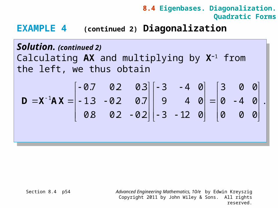
Solution. (continued 2)
Calculating AX and multiplying by X−1 from the left, we thus obtain
Solution. (continued 2)
Calculating AX and multiplying by X−1 from the left, we thus obtain
EXAMPLE 4 (continued 2) Diagonalization
8.4 Eigenbases. Diagonalization.Quadratic Forms
1
0.7 0.2 0.3 3 4 0 3 0 0
1.3 0.2 0.7 9 4 0 0 4 0 .
0.8 0.2 0.2 3 12 0 0 0 0
D X AX
Advanced Engineering Mathematics, 10/e by Edwin KreyszigCopyright 2011 by John Wiley & Sons. All rights reserved.
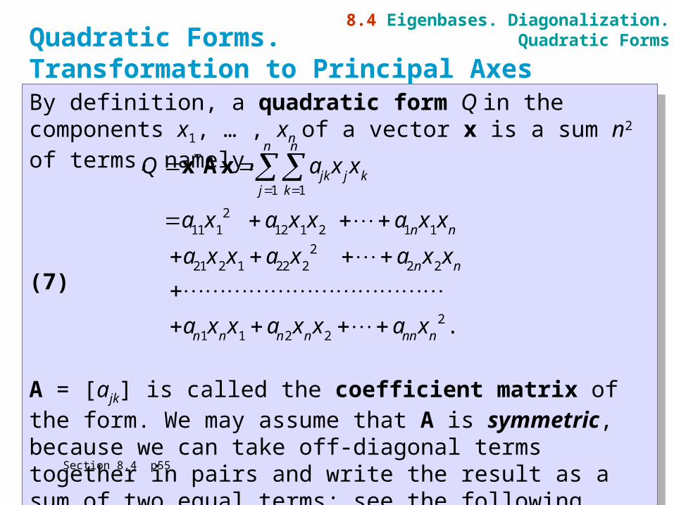
By definition, a quadratic form Q in the components x1, … , xn of a vector x is a sum n2 of terms, namely,
(7)
A = [ajk] is called the coefficient matrix of the form. We may assume that A is symmetric, because we can take off-diagonal terms together in pairs and write the result as a sum of two equal terms; see the following example.
By definition, a quadratic form Q in the components x1, … , xn of a vector x is a sum n2 of terms, namely,
(7)
A = [ajk] is called the coefficient matrix of the form. We may assume that A is symmetric, because we can take off-diagonal terms together in pairs and write the result as a sum of two equal terms; see the following example.Section 8.4 p55
Quadratic Forms. Transformation to Principal Axes
8.4 Eigenbases. Diagonalization.Quadratic Forms
1 1
211 1 12 1 2 1 1
221 2 1 22 2 2 2
21 1 2 2
.
n n
jk j kj k
n n
n n
n n n n nn n
Q a x x
a x a x x a x x
a x x a x a x x
a x x a x x a x
x Ax
T
Advanced Engineering Mathematics, 10/e by Edwin KreyszigCopyright 2011 by John Wiley & Sons. All rights reserved.
Section 8.4 p56
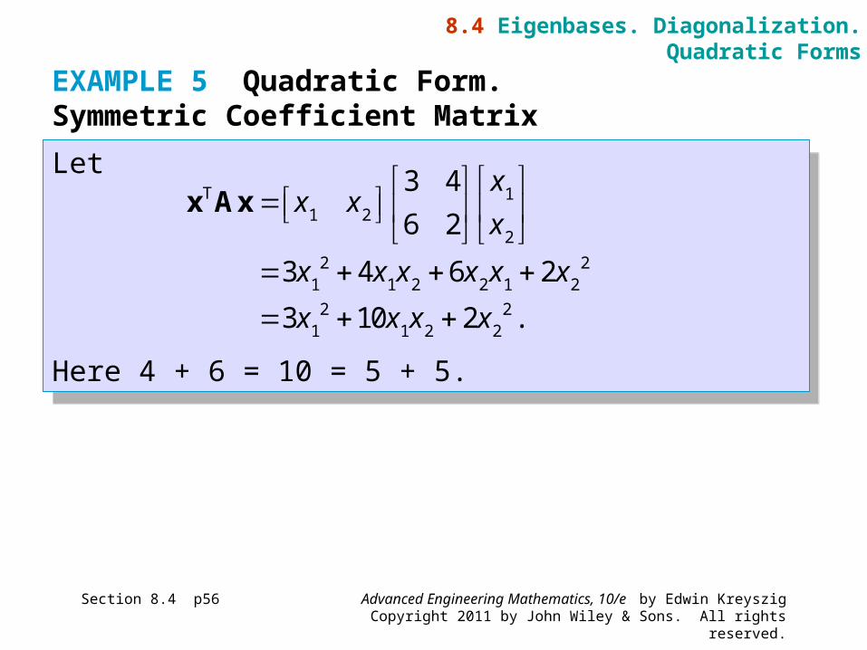
Let
Here 4 + 6 = 10 = 5 + 5.
Let
Here 4 + 6 = 10 = 5 + 5.
EXAMPLE 5 Quadratic Form. Symmetric Coefficient Matrix
8.4 Eigenbases. Diagonalization.Quadratic Forms
11 2
2
2 21 1 2 2 1 2
2 21 1 2 2
3 4
6 2
3 4 6 2
3 10 2 .
xx x
x
x x x x x x
x x x x
x AxT
Advanced Engineering Mathematics, 10/e by Edwin KreyszigCopyright 2011 by John Wiley & Sons. All rights reserved.
Section 8.4 p57
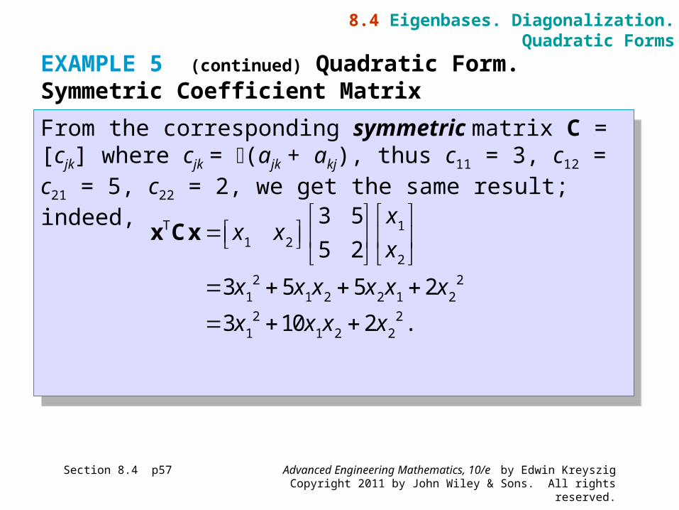
From the corresponding symmetric matrix C = [cjk] where cjk = (ajk + akj), thus c11 = 3, c12 = c21 = 5, c22 = 2, we get the same result; indeed,
From the corresponding symmetric matrix C = [cjk] where cjk = (ajk + akj), thus c11 = 3, c12 = c21 = 5, c22 = 2, we get the same result; indeed,
EXAMPLE 5 (continued) Quadratic Form. Symmetric Coefficient Matrix
8.4 Eigenbases. Diagonalization.Quadratic Forms
11 2
2
2 21 1 2 2 1 2
2 21 1 2 2
3 5
5 2
3 5 5 2
3 10 2 .
xx x
x
x x x x x x
x x x x
x CxT
Advanced Engineering Mathematics, 10/e by Edwin KreyszigCopyright 2011 by John Wiley & Sons. All rights reserved.
Section 8.4 p58
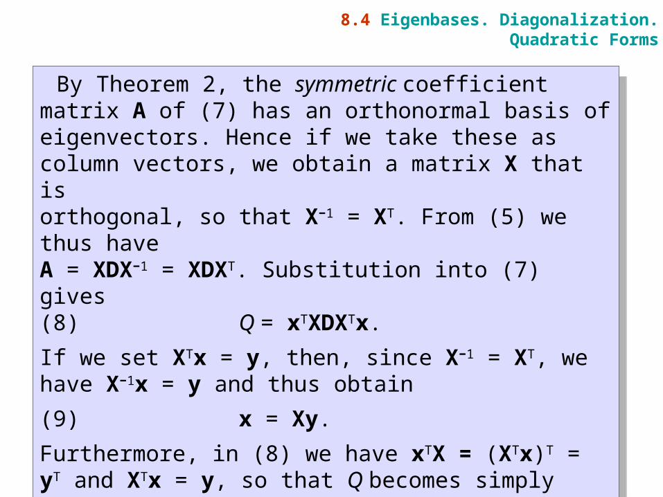
By Theorem 2, the symmetric coefficient matrix A of (7) has an orthonormal basis of eigenvectors. Hence if we take these as column vectors, we obtain a matrix X that isorthogonal, so that X−1 = XT. From (5) we thus have A = XDX−1 = XDXT. Substitution into (7) gives(8) Q = xTXDXTx.
If we set XTx = y, then, since X−1 = XT, we have X−1x = y and thus obtain
(9) x = Xy.
Furthermore, in (8) we have xTX = (XTx)T = yT and XTx = y, so that Q becomes simply
(10) Q = yTDy = λ1y12 + λ2y2
2 + … + λnyn2.
8.4 Eigenbases. Diagonalization.Quadratic Forms
Advanced Engineering Mathematics, 10/e by Edwin KreyszigCopyright 2011 by John Wiley & Sons. All rights reserved.
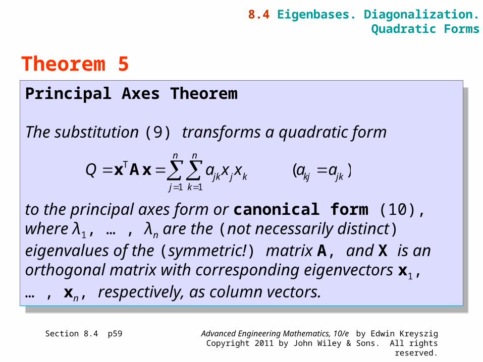
Principal Axes Theorem
The substitution (9) transforms a quadratic form
to the principal axes form or canonical form (10), where λ1, … , λn are the (not necessarily distinct) eigenvalues of the (symmetric!) matrix A, and X is an orthogonal matrix with corresponding eigenvectors x1, … , xn, respectively, as column vectors.
Section 8.4 p59
Theorem 5
8.4 Eigenbases. Diagonalization.Quadratic Forms
1 1
( )n n
jk j k kj jkj k
Q a x x a a
x AxT
Advanced Engineering Mathematics, 10/e by Edwin KreyszigCopyright 2011 by John Wiley & Sons. All rights reserved.
Section 8.4 p60
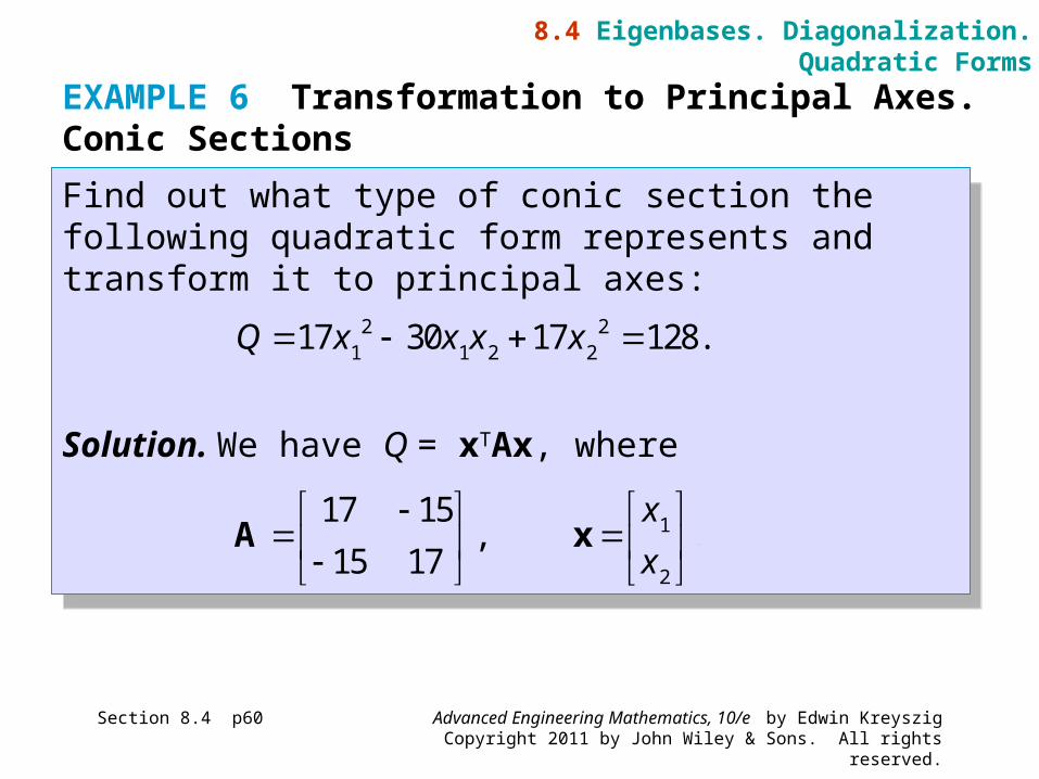
Find out what type of conic section the following quadratic form represents and transform it to principal axes:
Solution. We have Q = xTAx, where
Find out what type of conic section the following quadratic form represents and transform it to principal axes:
Solution. We have Q = xTAx, where
EXAMPLE 6 Transformation to Principal Axes. Conic Sections
8.4 Eigenbases. Diagonalization.Quadratic Forms
2 21 1 2 217 30 17 128.Q x x x x
1
2
17 15, .
15 17
x
x
A x
Advanced Engineering Mathematics, 10/e by Edwin KreyszigCopyright 2011 by John Wiley & Sons. All rights reserved.
Section 8.4 p61
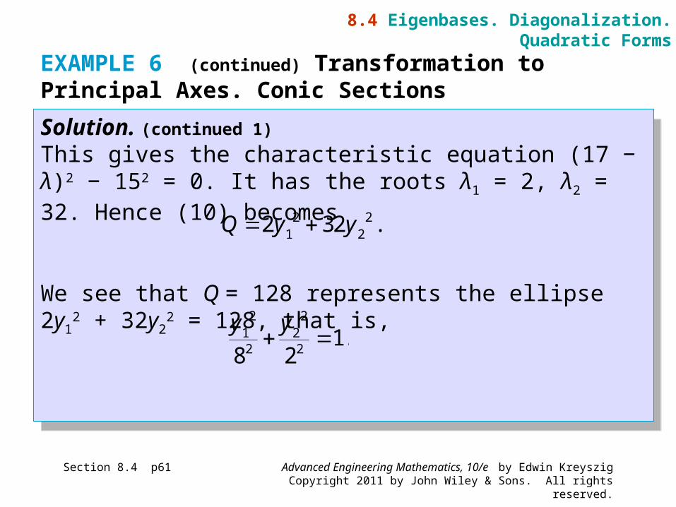
Solution. (continued 1)
This gives the characteristic equation (17 − λ)2 − 152 = 0. It has the roots λ1 = 2, λ2 = 32. Hence (10) becomes
We see that Q = 128 represents the ellipse 2y12 +
32y22 = 128, that is,
Solution. (continued 1)
This gives the characteristic equation (17 − λ)2 − 152 = 0. It has the roots λ1 = 2, λ2 = 32. Hence (10) becomes
We see that Q = 128 represents the ellipse 2y12 +
32y22 = 128, that is,
EXAMPLE 6 (continued) Transformation to Principal Axes. Conic Sections
8.4 Eigenbases. Diagonalization.Quadratic Forms
2 21 22 32 .Q y y
2 21 22 2
1.8 2
y y
Advanced Engineering Mathematics, 10/e by Edwin KreyszigCopyright 2011 by John Wiley & Sons. All rights reserved.
Section 8.4 p62
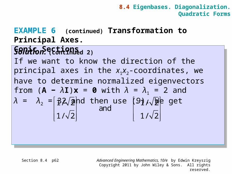
Solution. (continued 2)
If we want to know the direction of the principal axes in the x1x2-coordinates, we have to determine normalized eigenvectors from (A − λI)x = 0 with λ = λ1 = 2 and λ = λ2 = 32 and then use (9). We get
Solution. (continued 2)
If we want to know the direction of the principal axes in the x1x2-coordinates, we have to determine normalized eigenvectors from (A − λI)x = 0 with λ = λ1 = 2 and λ = λ2 = 32 and then use (9). We get
EXAMPLE 6 (continued) Transformation to Principal Axes. Conic Sections
8.4 Eigenbases. Diagonalization.Quadratic Forms
1/ 2 1/ 2 and
1/ 2 1/ 2
Advanced Engineering Mathematics, 10/e by Edwin KreyszigCopyright 2011 by John Wiley & Sons. All rights reserved.
Section 8.4 p63
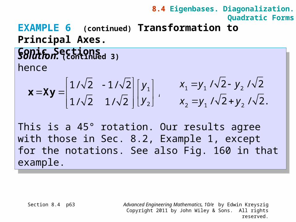
Solution. (continued 3)
hence
This is a 45° rotation. Our results agree with those in Sec. 8.2, Example 1, except for the notations. See also Fig. 160 in that example.
Solution. (continued 3)
hence
This is a 45° rotation. Our results agree with those in Sec. 8.2, Example 1, except for the notations. See also Fig. 160 in that example.
EXAMPLE 6 (continued) Transformation to Principal Axes. Conic Sections
8.4 Eigenbases. Diagonalization.Quadratic Forms
1
2
1/ 2 1/ 2,
1/ 2 1/ 2
y
y
x Xy 1 1 2
2 1 2
/ 2 / 2
/ 2 / 2.
x y y
x y y
Advanced Engineering Mathematics, 10/e by Edwin KreyszigCopyright 2011 by John Wiley & Sons. All rights reserved.
Section 8.5 p64
8.5 Complex Matrices and Forms. Optional
8.5 Complex Matrices and Forms. Optional
Advanced Engineering Mathematics, 10/e by Edwin KreyszigCopyright 2011 by John Wiley & Sons. All rights reserved.
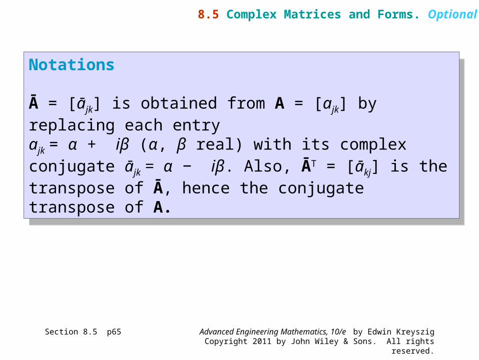
Notations
Ā = [ājk] is obtained from A = [ajk] by replacing each entryajk = α + iβ (α, β real) with its complex conjugate ājk = α − iβ. Also, ĀT = [ākj] is the transpose of Ā, hence the conjugate transpose of A.
Notations
Ā = [ājk] is obtained from A = [ajk] by replacing each entryajk = α + iβ (α, β real) with its complex conjugate ājk = α − iβ. Also, ĀT = [ākj] is the transpose of Ā, hence the conjugate transpose of A.
8.5 Complex Matrices and Forms. Optional
Section 8.5 p65
Advanced Engineering Mathematics, 10/e by Edwin KreyszigCopyright 2011 by John Wiley & Sons. All rights reserved.
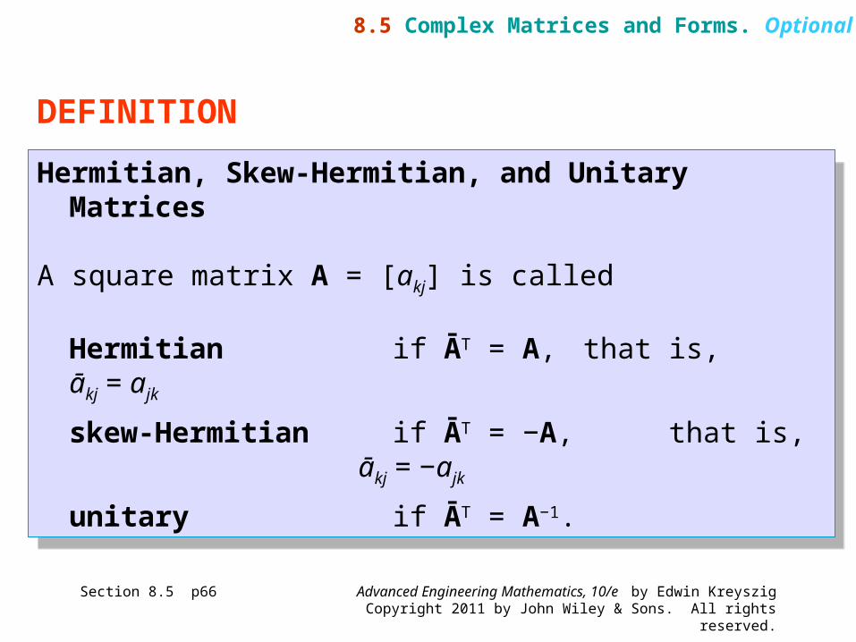
Hermitian, Skew-Hermitian, and Unitary Matrices
A square matrix A = [akj] is called
Hermitian if ĀT = A, that is, ākj = ajk
skew-Hermitian if ĀT = −A, that is, ākj = −ajk
unitary if ĀT = A−1.
Hermitian, Skew-Hermitian, and Unitary Matrices
A square matrix A = [akj] is called
Hermitian if ĀT = A, that is, ākj = ajk
skew-Hermitian if ĀT = −A, that is, ākj = −ajk
unitary if ĀT = A−1.
Section 8.5 p66
DEFINITION
8.5 Complex Matrices and Forms. Optional
Advanced Engineering Mathematics, 10/e by Edwin KreyszigCopyright 2011 by John Wiley & Sons. All rights reserved.
Section 8.5 p67
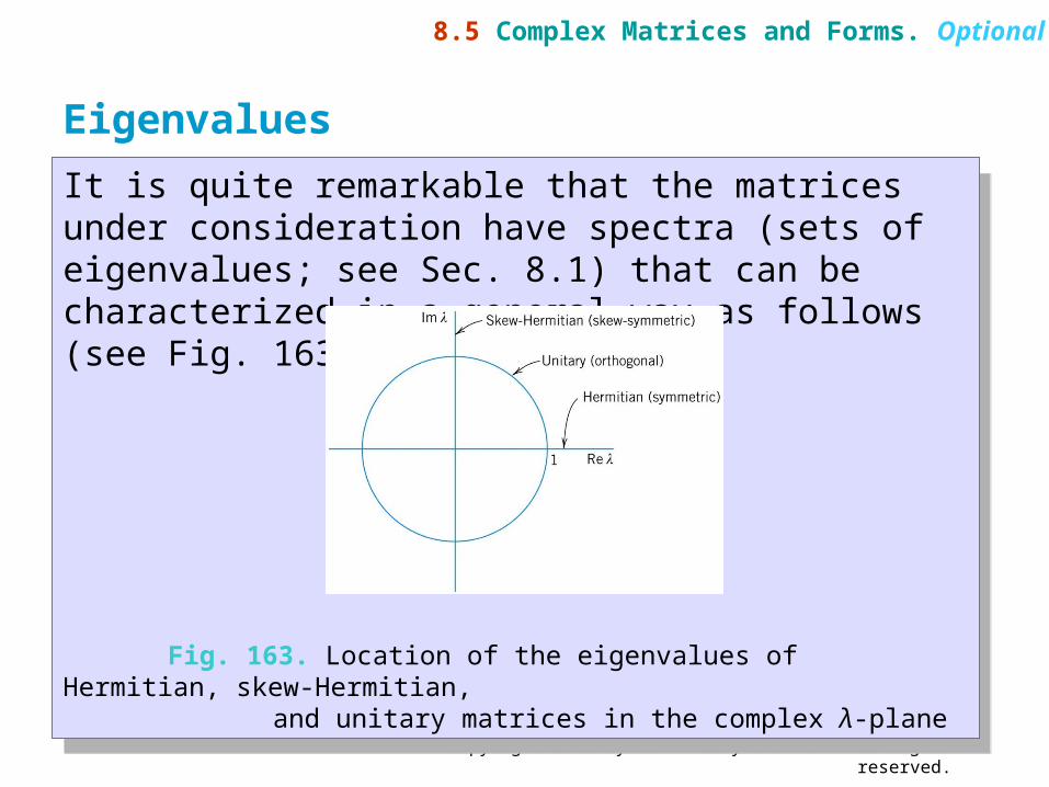
It is quite remarkable that the matrices under consideration have spectra (sets of eigenvalues; see Sec. 8.1) that can be characterized in a general way as follows (see Fig. 163).
Fig. 163. Location of the eigenvalues of Hermitian, skew-Hermitian,and unitary matrices in the complex λ-plane
It is quite remarkable that the matrices under consideration have spectra (sets of eigenvalues; see Sec. 8.1) that can be characterized in a general way as follows (see Fig. 163).
Fig. 163. Location of the eigenvalues of Hermitian, skew-Hermitian,and unitary matrices in the complex λ-plane
Eigenvalues
8.5 Complex Matrices and Forms. Optional
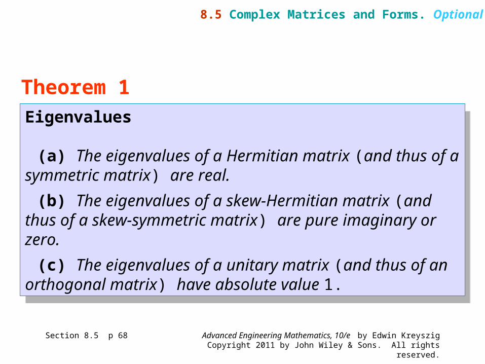
Advanced Engineering Mathematics, 10/e by Edwin KreyszigCopyright 2011 by John Wiley & Sons. All rights reserved.
Eigenvalues
(a) The eigenvalues of a Hermitian matrix (and thus of a symmetric matrix) are real.
(b) The eigenvalues of a skew-Hermitian matrix (and thus of a skew-symmetric matrix) are pure imaginary or zero.
(c) The eigenvalues of a unitary matrix (and thus of an orthogonal matrix) have absolute value 1.
Section 8.5 p 68
Theorem 1
8.5 Complex Matrices and Forms. Optional
Advanced Engineering Mathematics, 10/e by Edwin KreyszigCopyright 2011 by John Wiley & Sons. All rights reserved.
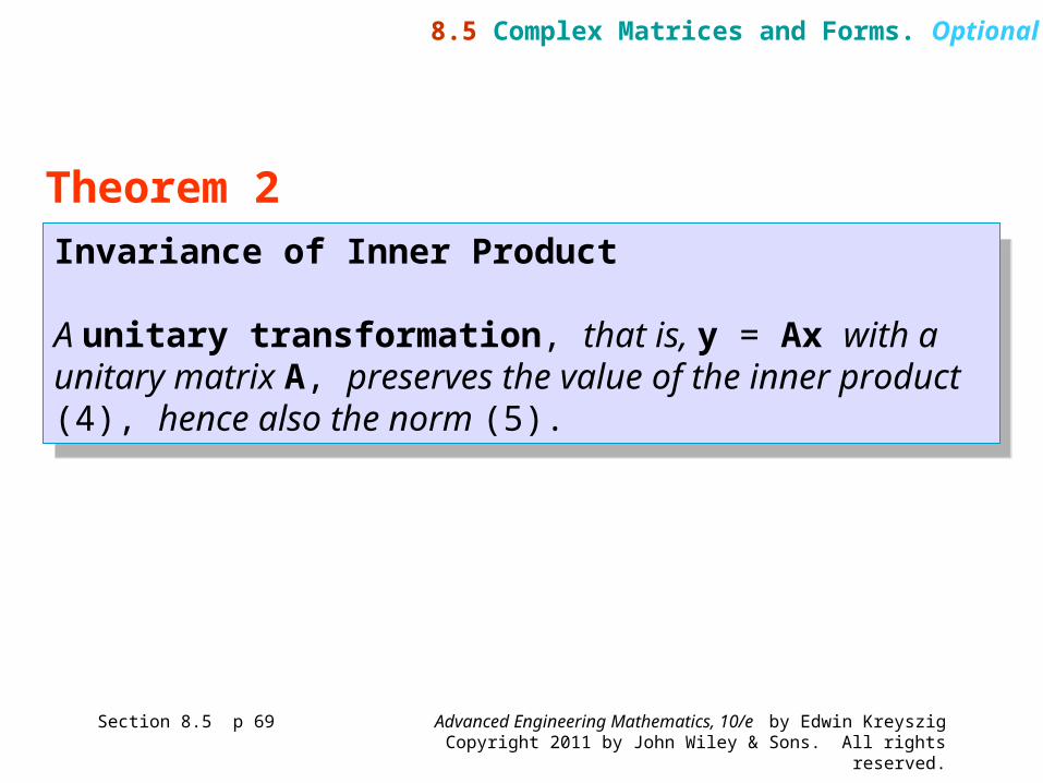
Invariance of Inner Product
A unitary transformation, that is, y = Ax with a unitary matrix A, preserves the value of the inner product (4), hence also the norm (5).
Invariance of Inner Product
A unitary transformation, that is, y = Ax with a unitary matrix A, preserves the value of the inner product (4), hence also the norm (5).
Section 8.5 p 69
Theorem 2
8.5 Complex Matrices and Forms. Optional
Advanced Engineering Mathematics, 10/e by Edwin KreyszigCopyright 2011 by John Wiley & Sons. All rights reserved.
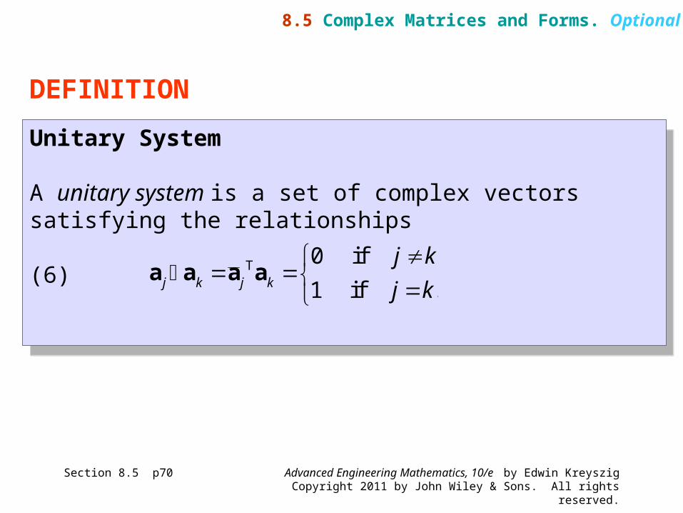
Unitary System
A unitary system is a set of complex vectors satisfying the relationships
(6)
Unitary System
A unitary system is a set of complex vectors satisfying the relationships
(6)
Section 8.5 p70
DEFINITION
8.5 Complex Matrices and Forms. Optional
0 if
1 if .j k j k
j k
j k
a a a a T
Advanced Engineering Mathematics, 10/e by Edwin KreyszigCopyright 2011 by John Wiley & Sons. All rights reserved.
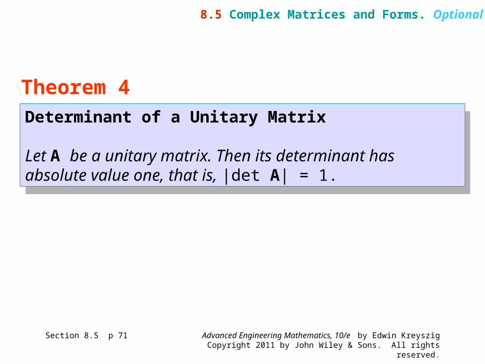
Determinant of a Unitary Matrix
Let A be a unitary matrix. Then its determinant has absolute value one, that is, |det A| = 1.
Determinant of a Unitary Matrix
Let A be a unitary matrix. Then its determinant has absolute value one, that is, |det A| = 1.
Section 8.5 p 71
Theorem 4
8.5 Complex Matrices and Forms. Optional
Advanced Engineering Mathematics, 10/e by Edwin KreyszigCopyright 2011 by John Wiley & Sons. All rights reserved.
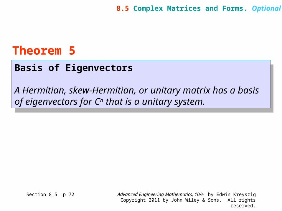
Basis of Eigenvectors
A Hermitian, skew-Hermitian, or unitary matrix has a basis of eigenvectors for Cn that is a unitary system.
Basis of Eigenvectors
A Hermitian, skew-Hermitian, or unitary matrix has a basis of eigenvectors for Cn that is a unitary system.
Section 8.5 p 72
Theorem 5
8.5 Complex Matrices and Forms. Optional
Advanced Engineering Mathematics, 10/e by Edwin KreyszigCopyright 2011 by John Wiley & Sons. All rights reserved.
Section 8.5 p73
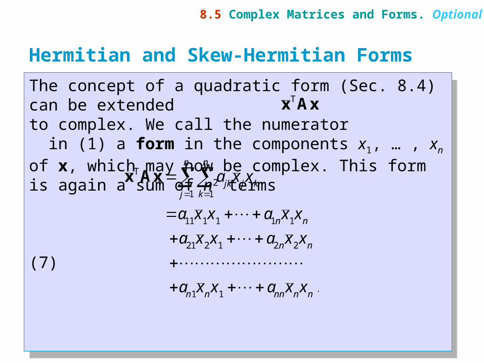
The concept of a quadratic form (Sec. 8.4) can be extendedto complex. We call the numerator in (1) a form in the components x1, … , xn of x, which may now be complex. This form is again a sum of n2 terms
(7)
The concept of a quadratic form (Sec. 8.4) can be extendedto complex. We call the numerator in (1) a form in the components x1, … , xn of x, which may now be complex. This form is again a sum of n2 terms
(7)
Hermitian and Skew-Hermitian Forms
8.5 Complex Matrices and Forms. Optional
x AxT
1 1
11 1 1 1 1
21 2 1 2 2
1 1 .
n n
jk j kj k
n n
n n
n n nn n n
a x x
a x x a x x
a x x a x x
a x x a x x
x Ax
T
Advanced Engineering Mathematics, 10/e by Edwin KreyszigCopyright 2011 by John Wiley & Sons. All rights reserved.
Section 8.5 p74
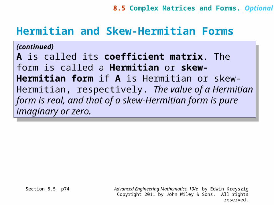
(continued)
A is called its coefficient matrix. The form is called a Hermitian or skew-Hermitian form if A is Hermitian or skew-Hermitian, respectively. The value of a Hermitian form is real, and that of a skew-Hermitian form is pure imaginary or zero.
(continued)
A is called its coefficient matrix. The form is called a Hermitian or skew-Hermitian form if A is Hermitian or skew-Hermitian, respectively. The value of a Hermitian form is real, and that of a skew-Hermitian form is pure imaginary or zero.
Hermitian and Skew-Hermitian Forms
8.5 Complex Matrices and Forms. Optional

Advanced Engineering Mathematics, 10/e by Edwin KreyszigCopyright 2011 by John Wiley & Sons. All rights reserved.
SUMMARY OF CHAPTER 8Linear Algebra:
Matrix Eigenvalue Problems
SUMMARY OF CHAPTER 8Linear Algebra:
Matrix Eigenvalue Problems
Section 8.Summary p75
Advanced Engineering Mathematics, 10/e by Edwin KreyszigCopyright 2011 by John Wiley & Sons. All rights reserved.
Section 8.Summary p76
SUMMARY OF CHAPTER 8Linear Algebra: Matrix Eigenvalue Problems
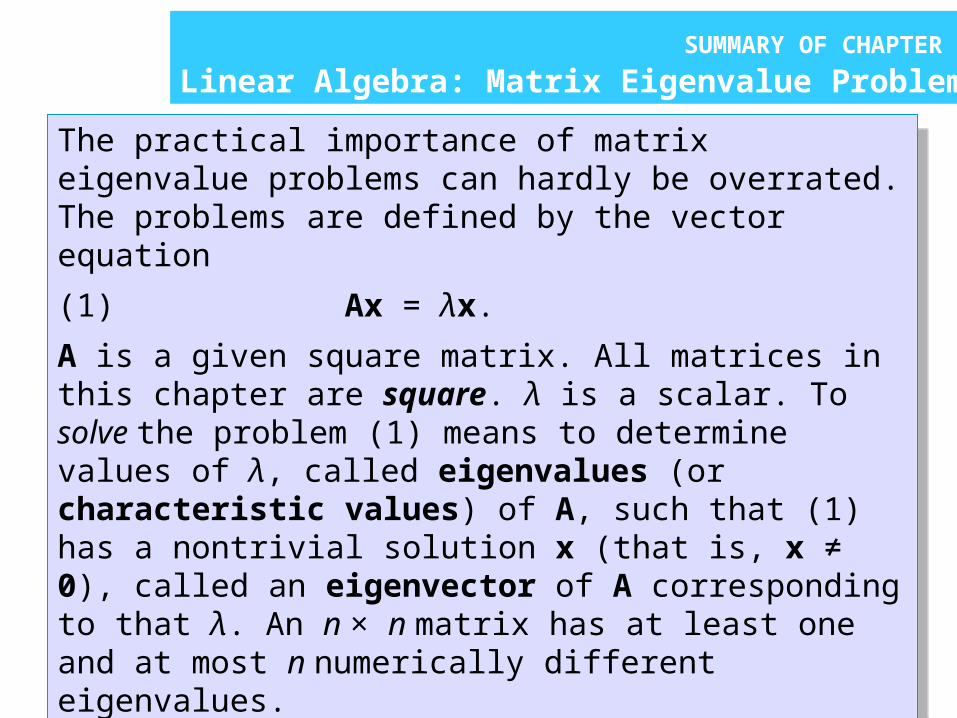
The practical importance of matrix eigenvalue problems can hardly be overrated. The problems are defined by the vector equation
(1) Ax = λx.
A is a given square matrix. All matrices in this chapter are square. λ is a scalar. To solve the problem (1) means to determine values of λ, called eigenvalues (or characteristic values) of A, such that (1) has a nontrivial solution x (that is, x ≠ 0), called an eigenvector of A corresponding to that λ. An n × n matrix has at least one and at most n numerically different eigenvalues.
Advanced Engineering Mathematics, 10/e by Edwin KreyszigCopyright 2011 by John Wiley & Sons. All rights reserved.
Section 8.Summary p77
SUMMARY OF CHAPTER 8Linear Algebra: Matrix Eigenvalue Problems
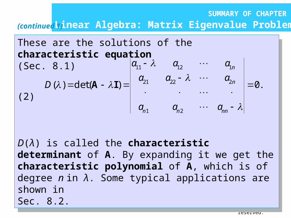
These are the solutions of the characteristic equation (Sec. 8.1)
(2)
D(λ) is called the characteristic determinant of A. By expanding it we get the characteristic polynomial of A, which is of degree n in λ. Some typical applications are shown in Sec. 8.2.
These are the solutions of the characteristic equation (Sec. 8.1)
(2)
D(λ) is called the characteristic determinant of A. By expanding it we get the characteristic polynomial of A, which is of degree n in λ. Some typical applications are shown in Sec. 8.2.
11 12 1
21 22 2
1 2
( ) det( ) 0.
n
n
n n nn
a a a
a a aD
a a a
A I
(continued 1)
Advanced Engineering Mathematics, 10/e by Edwin KreyszigCopyright 2011 by John Wiley & Sons. All rights reserved.
Section 8.Summary p78
SUMMARY OF CHAPTER 8Linear Algebra: Matrix Eigenvalue Problems
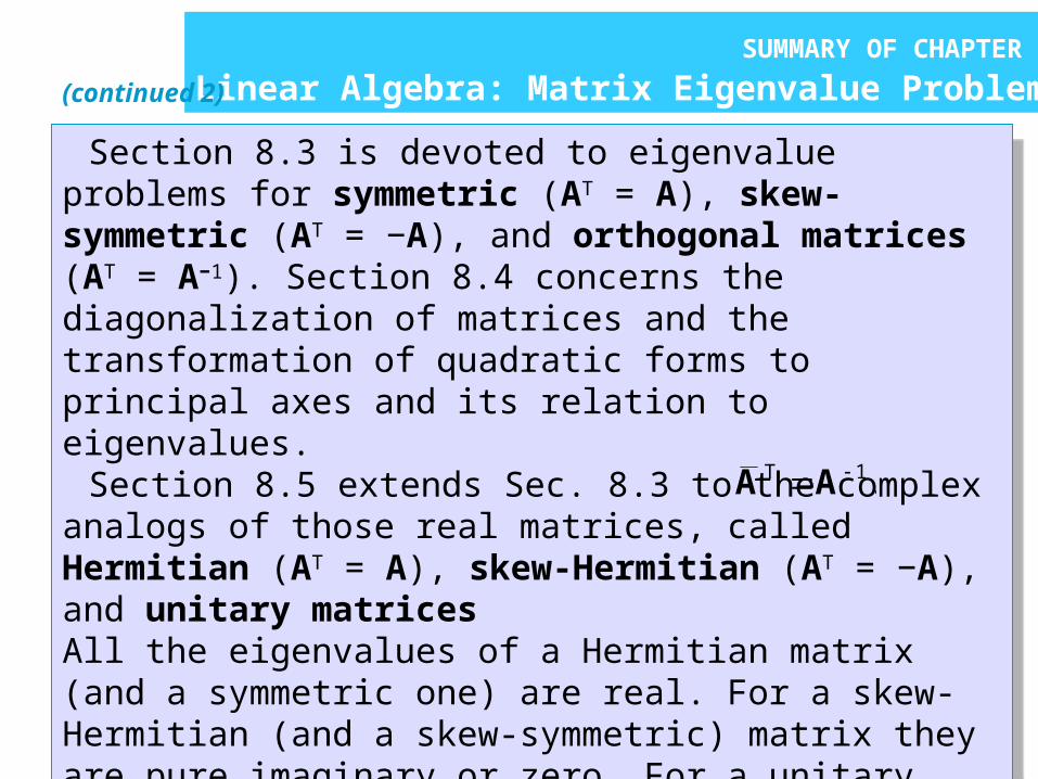
Section 8.3 is devoted to eigenvalue problems for symmetric (AT = A), skew-symmetric (AT = −A), and orthogonal matrices (AT = A−1). Section 8.4 concerns the diagonalization of matrices and the transformation of quadratic forms to principal axes and its relation to eigenvalues.
Section 8.5 extends Sec. 8.3 to the complex analogs of those real matrices, called Hermitian (AT = A), skew-Hermitian (AT = −A), and unitary matrices All the eigenvalues of a Hermitian matrix (and a symmetric one) are real. For a skew-Hermitian (and a skew-symmetric) matrix they are pure imaginary or zero. For a unitary (and an orthogonal) matrix they have absolute value 1.
(continued 2)
1.A AT