Advanced Economic Analysis - NASA Why should Federal Government consider time value of money? •...
107
Advanced Economic Analysis Marc Greenberg Cost Analysis Division, NASA William Laing Technomics, Inc. https://ntrs.nasa.gov/search.jsp?R=20130013014 2018-06-14T04:38:26+00:00Z
Transcript of Advanced Economic Analysis - NASA Why should Federal Government consider time value of money? •...

Advanced Economic Analysis
Marc Greenberg
Cost Analysis Division, NASA
William Laing
Technomics, Inc.
https://ntrs.nasa.gov/search.jsp?R=20130013014 2018-06-14T04:38:26+00:00Z
2
Learning Objectives • Define an economic analysis (EA)
• Explain why discounting calculations are performed
• Show how discount factors are calculated – End-of-Year (EOY) and Middle-of-Year (MOY) conventions
• Discuss the steps of an EA
• Demonstrate the steps of an EA using examples
• Develop cash flow diagrams for feasible alternatives
• Apply discount factors to cash flows
• Calculate Economic Analysis measures-of-merit such as: – Net Present Value (NPV)
– Equivalent Uniform Annual Worth (EUAW)
– Non-monetary Benefits
• Discuss sensitivity analysis & provide an example
• Discuss how to recommend the most preferred alternative & provide an example – gives the decision maker tools to make a more informed decision
3
What is Economic Analysis (EA)?
• An EA is a systematic approach to the problem of choosing the best method of allocating scarce resources to achieve a given objective. [Ref. DoD 7041.3]
– There are alternative ways to meet an objective • Each alternative requires the use of resources and
produces certain results
An EA helps guide decisions on the “worth” of
pursuing an action that departs from status quo
… an EA is the crux of decision-support
4
The Concept of Discounting

5
Time Value of Money
• Stems from natural human instinct for finding more
pleasure from money in hand today than the firm
expectation of acquiring an exactly equal amount
(corrected for inflation) at some time in future
• When we say money has ―time value,‖ we mean that
a dollar to be paid (received) today is worth more
than a dollar to be paid (received) at any future time
• Time value arises because of
– the opportunity to earn interest on money in hand or
– the cost of paying interest on borrowed capital.
6
Time Value of Money (Example)
• Would you rather have $10,000 in hand today or a legal document entitling a withdrawal of $10,000 (plus increment for any inflation) from a bank a year from now? – The logical answer is for you to prefer to receive $10,000 today
because there is no change in ―value‖ a year from now.
• What if another bank promises you (depositing $10,000) to receive $11,000 a year from now? Is the ―value‖ of waiting a year is worth the $1,000 in accumulated interest? – It would not be worth it if a $10,000 investment in the stock market
yields 11% return over the next year.
– Your $10,000 would have grown to $11,100 a year from now.
– Therefore, the time-value-of-money increment would have been $1,100 instead of $1,000

7
Why should Federal Government
consider time value of money?
• Government is not a profit-making entity. Some argue that time value of money does not apply because – money not immediately spent on one project would be spent on
another …
– public funds are not invested at interest as in the private sector.
• However, money used by the government are funds kept out of the civilian economy. – such public funds do not grow; an opportunity cost is incurred
• The government is also concerned with the cost of capital when in deficit financing. – projects should produce returns in excess of borrowing cost.
8
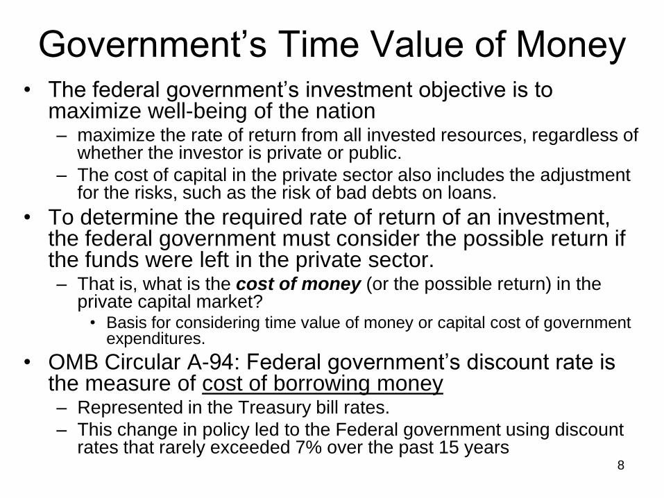
Government‘s Time Value of Money • The federal government‘s investment objective is to
maximize well-being of the nation – maximize the rate of return from all invested resources, regardless of
whether the investor is private or public.
– The cost of capital in the private sector also includes the adjustment for the risks, such as the risk of bad debts on loans.
• To determine the required rate of return of an investment, the federal government must consider the possible return if the funds were left in the private sector. – That is, what is the cost of money (or the possible return) in the
private capital market? • Basis for considering time value of money or capital cost of government
expenditures.
• OMB Circular A-94: Federal government‘s discount rate is the measure of cost of borrowing money – Represented in the Treasury bill rates.
– This change in policy led to the Federal government using discount rates that rarely exceeded 7% over the past 15 years

9
Interest versus Inflation • Inflation accounts for the loss of the purchasing
power of a dollar due to the general rise of prices in the economy.
• Interest is a measure of the time-value-of-money (monetary value of deferred consumption) – The time-value-of-money accounts for the fact that a
dollar today is worth more to us than a dollar received in the future, say a year from now.
– We can invest the dollar we get today, and in a year, we will have more than a dollar because we have earned interest on the investment.
– Conversely, when we must pay out money, we would prefer to pay in the future, rather than now because we can earn interest on the money while we hold it.

10
Interest and Interest Rate
• Two terms used almost synonymously
when discussing the future value of
money: interest and interest rate.
– Interest is expressed in dollars and represents
the money paid or received over time.
– The interest rate is a percentage that
expresses the fraction of cost or return on the
principal over time.

11
Interest Rate (Discount Rate)
• For most federal EAs the specific interest (discount) rate to use is directed by OMB and DoD directives. Interest rate (i) is: – expressed as a percent (%) or decimal (0.00)
– assessed on the dollar balance
– stated for a specified period of time (usually a year)
– based on the project life and type of analysis,
• e.g. constant dollar or current dollar
• OMB Circular A-94 prescribes specific interest rates depending on the project term. – Different rates are also used if the analysis is in base year
(without inflation) or then-year (with inflation) dollars.

12
Interest: Nominal and Real Rates
• Nominal rate: rate of return used against payments that include inflation (i.e. cash flows in current or then year dollars). – most loans and returns provided by financial institutions (e.g., banks,
credit card companies, mortgage companies, etc.) are advertised as nominal rates.
• Real rate: equals the nominal rate adjusted to eliminate the effect of anticipated inflation (or deflation) – used for payments that are in terms of stable purchasing power
(cash flows measured in constant or base year dollars).
– primarily used to perform EAs with cash flows depicted in constant (base year) dollars.
All examples in this lesson assume “Real Rates”

13
Compound Interest Formula
• Interest charged (or received) over a period is based upon the balance of principal and interest of the previous period.
• Future value based on compound interest for a single payment (receipt) is depicted as:
(1 ) nFV PV i
FV = future value; the total amount received or repaid
PV = present value; principal amount lent or borrowed
n = number of interest periods (e.g. years)
i = interest rate per interest period

14
Compound Interest (Example) • Suppose you had $1,000 today (PV) and invested it at an
annual interest rate of 10%. Because this PV of $1,000 accumulates $100 of interest over a year, you would collect $1,100 in one year (FV). You can calculate your FV as:
• What if you decided to withdraw the money in five years?
Assuming interest rate is fixed at 10%, your FV becomes:
• $1,000 was ―invested‖ at an interest rate of 10% to become
―worth‖ $1,611 just five years later.
15
Present Value (PV) & Discounting
A dollar today, worth more than a dollar in the future, can be measured in terms of accrued compound interest = Time-value-of-money
Such mechanics of time-value-of-money can also be applied in reverse.
• That is … you can estimate the equivalent value of a dollar held now (Present Value or PV) based on a given future dollar value (Future Value or FV)
• This adjustment to a common point in time (typically from FV to PV) is called “discounting”
16
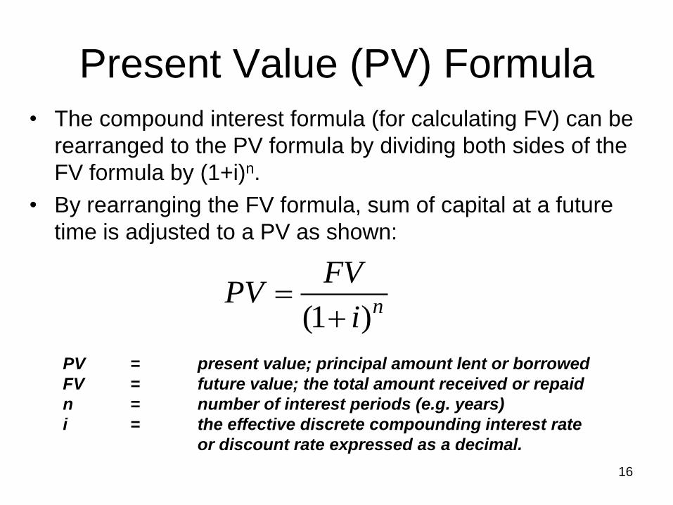
Present Value (PV) Formula
• The compound interest formula (for calculating FV) can be
rearranged to the PV formula by dividing both sides of the
FV formula by (1+i)n.
• By rearranging the FV formula, sum of capital at a future
time is adjusted to a PV as shown:
(1 )
n
FVPV
i
PV = present value; principal amount lent or borrowed
FV = future value; the total amount received or repaid
n = number of interest periods (e.g. years)
i = the effective discrete compounding interest rate
or discount rate expressed as a decimal.

17
PV Formula (Example 1)
• Suppose you owed $1,000 a year from now, and your bank offers a 1-yr CD account rate of 10%,
• If you put away $909.09 today, you would meet that obligation. – $909.09 (PV) can be invested for 1 year to accrue
principal plus interest = $1,000 (FV).
• Using the PV equation, you can calculate the PV of such a future debt or receipt (FV) as:
1
$1,000 = = $909.09
(1 ) (1 0.10)
n
FVPV
i

18
PV Formula (Example 2)
• You know you‘ll need a car after graduating college
(in 4 years) and you want to buy one in cash. You
estimate you‘ll need $20,000 in 4 years. Assuming
a discount rate of 10%, if you invested $13,660
now, you would have $20,000 in four years:
• This example demonstrates how a future
―lump sum‖ expense of $20,000 is equivalent
to spending $13,660 today.

19
What is Discount Rate? … reflects the opportunity cost of making an investment
… equals the interest rate used to determine the present value of a future cash stream – an average interest rate based upon marketable U.S. Treasury securities of
similar maturity to the project term of the expenditure under consideration
For each investment, the Federal Government has 2 options for acquiring money. It can:
… borrow money. Therefore, it must pay interest. – The amount Federal Government has to pay in interest to borrow
money is the opportunity cost of borrowing
… collect more taxes. Taxpayers lose ability to earn interest on private sector investments they can no longer make. – The lost interest is the opportunity cost of taxation. .
The government's cost of borrowing money is the basis
for discount rates used in conducting an EA.
20
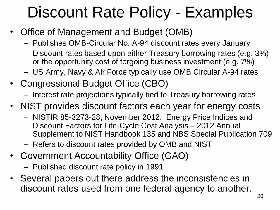
Discount Rate Policy - Examples • Office of Management and Budget (OMB)
– Publishes OMB-Circular No. A-94 discount rates every January
– Discount rates based upon either Treasury borrowing rates (e.g. 3%) or the opportunity cost of forgoing business investment (e.g. 7%)
– US Army, Navy & Air Force typically use OMB Circular A-94 rates
• Congressional Budget Office (CBO) – Interest rate projections typically tied to Treasury borrowing rates
• NIST provides discount factors each year for energy costs – NISTIR 85-3273-28, November 2012: Energy Price Indices and
Discount Factors for Life-Cycle Cost Analysis – 2012 Annual Supplement to NIST Handbook 135 and NBS Special Publication 709
– Refers to discount rates provided by OMB and NIST
• Government Accountability Office (GAO) – Published discount rate policy in 1991
• Several papers out there address the inconsistencies in discount rates used from one federal agency to another.

21
Discount Rate Conventions Payment is administratively made
• End-of-Year (EOY): At the end of the year (period)
• Middle-of-Year (MOY): At the middle of a year (period)
• Beginning-of-Year (BOY): At the beginning of year (period)
• Continuous: Payments or compounding are continuous and are not in discrete payments or periods – Example: personnel or equipment operate 24 hours per day, 7 days
per week, every day of the year
• We will apply two most common rates: EOY and MOY. – EOY: assume for investments or receipts (at year 0), for salvage value
or disposal costs (at end-of-service life) unless otherwise noted
– MOY: assume for all other expenditures unless otherwise noted

22
Discount Factor Formula Based on EOY Convention 1
PV = FV * EOY Discount Factor
1
(1 )
nPV FV
i
1 = EOY Discount Factor
(1 )niWe define …
Substituting, we get …
Present Value formula for EOY Payments (slide 23):
1. For Middle-of-Year discount factor, change denominator exponent from n to (n-0.5)

23
EOY Discount Factor Example
• Given a discount rate, i = 10%, over a period, n = 5 years, the discount factor can be calculated as:
5
1EOY Discount Factor 0.6209
(1 0.10)
PV = FV * EOY Discount Factor
PV = $10,000 * 0.6209 = $6,209
• Applying EOY discount factor to your car‘s salvage value (@ year n=5), converts the car‘s Future Value (FV) of $10,000 to a Present Value (PV) of $6,209:

24
The Economic Analysis
Process

25
EA Viewpoint
• Generally reflects policy, rationale & processes
w/in federal agencies (DoD & non-DoD)
• Costs and benefits must be viewed from the
perspective of the federal government as a
whole.
– EA cash flows are not limited to only the costs
and benefits incurred by the organization for
which the analysis is being done.
26
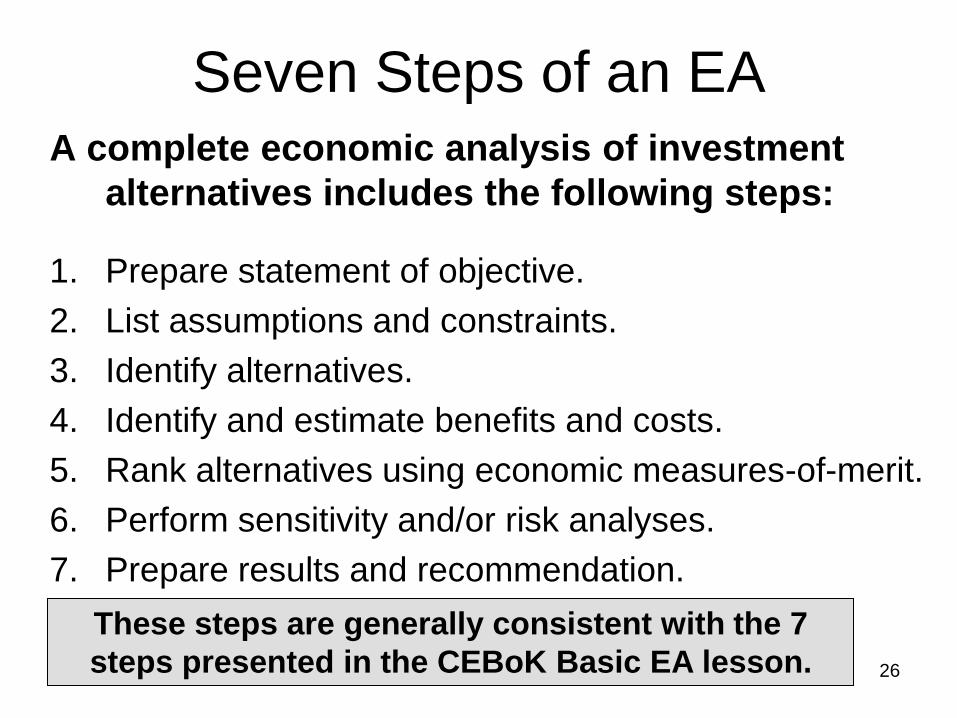
Seven Steps of an EA A complete economic analysis of investment
alternatives includes the following steps:
1. Prepare statement of objective.
2. List assumptions and constraints.
3. Identify alternatives.
4. Identify and estimate benefits and costs.
5. Rank alternatives using economic measures-of-merit.
6. Perform sensitivity and/or risk analyses.
7. Prepare results and recommendation.
These steps are generally consistent with the 7
steps presented in the CEBoK Basic EA lesson.

27
Iterative Nature of an EA
There are many interrelationships among the steps in the EA process. Rather than performing each step in order to completion, the steps may be revisited during the analysis (as shown below).
1. OBJECTIVE
2. ASSUMPTIONS
& CONSTRAINTS
3. ALTERNATIVES
4a. BENEFITS
4b. COSTS
5. RANK
ALTERNATIVES
6. SENSITIVITY &
RISK ANALYSIS
7. PREPARE RESULTS
& RECOMMENDATION

28
Step 1: Prepare Statement of Objective
• The Problem and Requirement.
– You usually get this information from a boss
who tells you to go fix a problem.
– The analyst may be at a disadvantage
because the ―real problem‖ as seen by higher
headquarters may not be obvious to the team
assigned to do the study.

29
Step 1: Prepare Statement of Objective The Problem and Requirement
A project is usually proposed to correct a deficiency
Some deficiencies that might prompt a project are 1. New functional requirement due to new mission or mission change
2. Space shortage
3. Engineering deficiency
4. Environmental, health, safety, fire protection, or security problem
5. Excessive operations and maintenance (O&M) costs
6. Functional inadequacy (e.g. HVAC system not right-sized for facility)
7. Inefficient condition (e.g. wasting energy or space)
Often a project identified to meet one requirement
may be expanded to meet others

30
Step 1: Prepare Statement of Objective
A good objective statement should consist of
three parts:
1. Product or service to be provided
2. Measurement system
3. Selection criteria
THIS IS THE MOST IMPORTANT STEP
Should involve both the decision maker and analyst
31
Step 1: Prepare Statement of Objective A. Product or service to be provided
• What will be provided, manufactured, produced,
procured or delivered.
– First, consider the mission or function desired.
Although it doesn‘t seem very well defined yet, it is
only because the alternatives more readily define the
product or service.
– The wording of the objective statement is critical. Be
specific enough to include the problem to be
addressed yet broad enough to pick up all feasible
alternatives.
– Be careful not to word the objective statement to lead
toward any one alternative.

32
Step 1: Prepare Statement of Objective B. Measurement system
• Standard by which the product or service to be
provided will be measured
– stated in terms of a standard, regulation, or building
code, or goal against which the results of the selected
problem solution can be measured.
• You must be able to measure the output in order
to determine the attainment of the goal
– Ex: Meet space requirement of 30 sq ft per employee

33
Step 1: Prepare Statement of Objective C. Selection Criteria
• Financial Comparisons
– Total Project Cost, Net Present Value (NPV),
Equivalent Uniform Annual Worth (EUAW),
Savings Investment Ratio (SIR), Benefit / Cost
Ratio (BCR), etc.
• Non-financial Comparisons
– Decision analysis scores typically based on
expert judgment
– Weight and score decision criteria, pair-wise
comparison methods, Delphi approach, etc.

34
Step 1: Prepare Statement of Objective Final Note
• State objective in quantifiable terms to greatest extent possible
– Makes it easier to compare and rank alternatives
• Performance measurement criteria need to be established
– So that relative costs and benefits of each alternative can be compared and tied directly to objective
• Word of caution: there is a practical limit on the depth of the statement of the functional need.
– Otherwise, the study might become unmanageable.
– Has sub-optimization so narrowed the scope of the problem that the real problem has been missed or worthwhile alternatives excluded?
A method of verifying the adequacy of objective statement
is to raise the project one level (see next slide … )
35
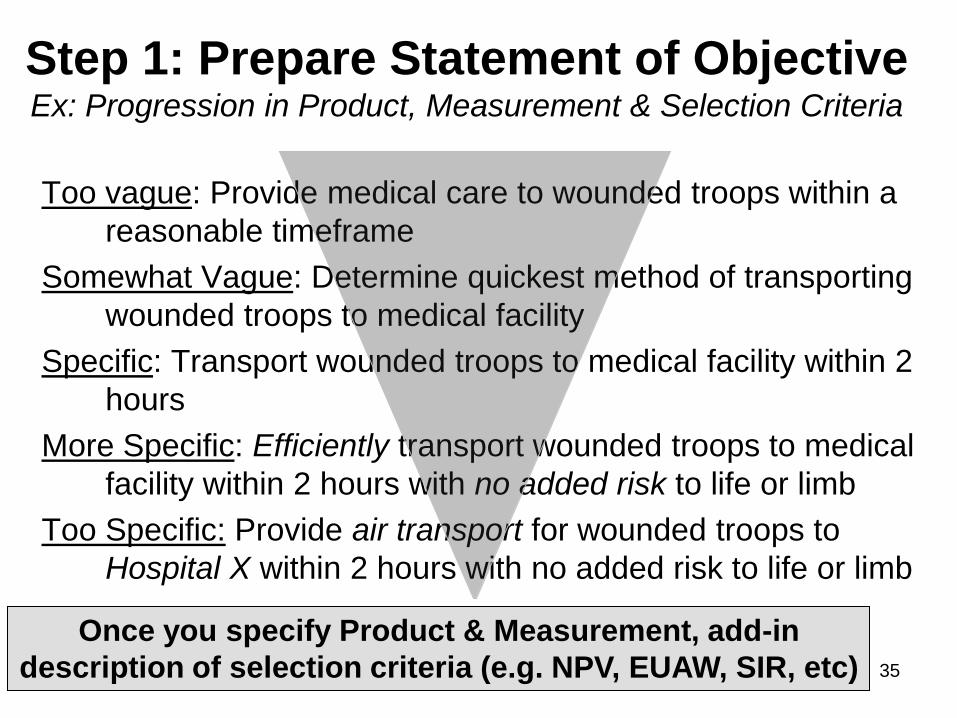
Step 1: Prepare Statement of Objective Ex: Progression in Product, Measurement & Selection Criteria
Too vague: Provide medical care to wounded troops within a
reasonable timeframe
Somewhat Vague: Determine quickest method of transporting
wounded troops to medical facility
Specific: Transport wounded troops to medical facility within 2
hours
More Specific: Efficiently transport wounded troops to medical
facility within 2 hours with no added risk to life or limb
Too Specific: Provide air transport for wounded troops to
Hospital X within 2 hours with no added risk to life or limb
Once you specify Product & Measurement, add-in
description of selection criteria (e.g. NPV, EUAW, SIR, etc)

36
Step 2: List assumptions and constraints
• This step enables you to weed out infeasible alternatives early.
• List only those assumptions which are absolutely necessary
– the more assumptions, the more chances to introduce uncertainty
• Identify limitations in the scope of the study
– such as limited timeframe or manpower to perform the study

37
Step 2a: List assumptions
The following items, by nature of their uncertainty, qualify as assumptions:
• Any future events
• Future economic assumptions
• Inflation factors
• Costs and benefits
• Projected workload
• Estimated economic life
• Period of analysis
• Changes to requirements
38
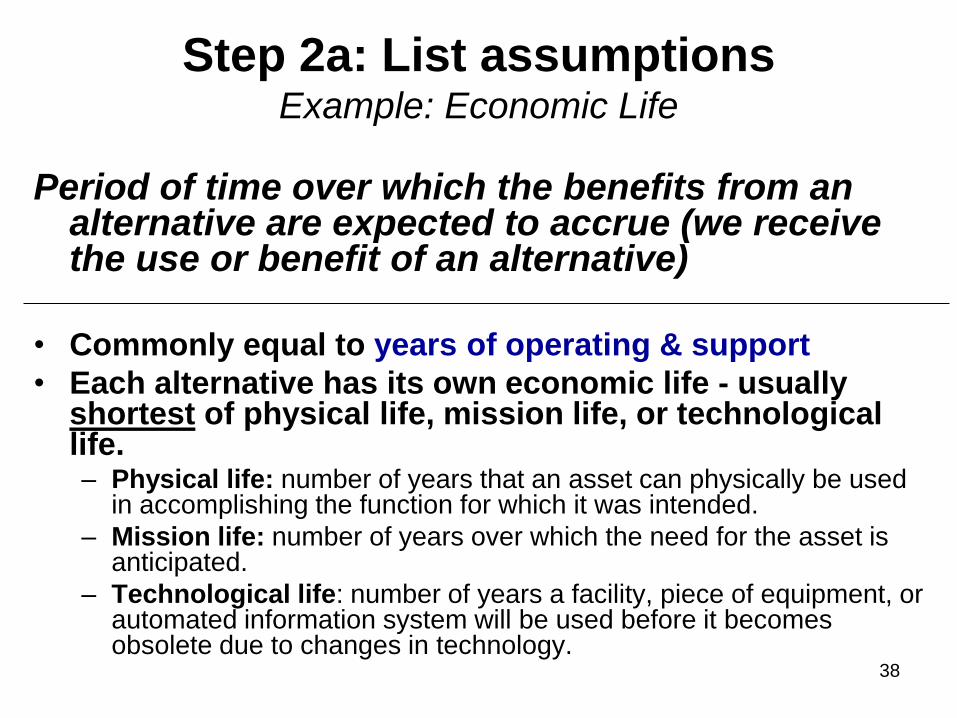
Step 2a: List assumptions Example: Economic Life
Period of time over which the benefits from an alternative are expected to accrue (we receive the use or benefit of an alternative)
• Commonly equal to years of operating & support
• Each alternative has its own economic life - usually shortest of physical life, mission life, or technological life. – Physical life: number of years that an asset can physically be used
in accomplishing the function for which it was intended.
– Mission life: number of years over which the need for the asset is anticipated.
– Technological life: number of years a facility, piece of equipment, or automated information system will be used before it becomes obsolete due to changes in technology.

39
Step 2a: List assumptions Example: Economic Life
• Program Office: Software requirements to support
combat system from FY08 through FY19 (Software
Mission Life = 12 years).
• Vendor A proposes ―Generic Software‖ that will be
obsolete in 4 years
– Program will benefit from software use from FY08 – 11
• Vendor B proposes ―Super Software‖ that will
become obsolete in 8 years
– Program will benefit from software use from FY08 - 15
Economic life is constrained to four years for one
alternative and eight years for the other alternative.

40
Step 2a: List assumptions Example: Period of Analysis
Starts from the year the first costs are incurred for each alternative and ends in the last year costs are incurred for that alternative. – Since it includes disposal costs, the period of
analysis may extend for some number of years beyond the end of economic life.

41
Step 2b: List constraints
• Size or range of the manager‘s ―operating area‖ are dependent upon total organizational freedom as well as the decision-maker‘s position within the organization.
• There may also be … – constraining organizational policies or procedures
– budgetary, funding or manpower considerations.
– restrictions caused by production (or other types of) deadlines
– limited amount of working area for team management & staff
• Whatever their particular characteristics, these external constraints or barriers … – are beyond the control of the analyst or manager and
– limit the number of feasible solutions to a given problem

42
Step 2: List constraints Examples
You must list constraints because:
• They are conditions that bind the analysis and
• They influence the generation of alternatives
Some constraints might be:
• budget • milestones
• funding • schedules or deadlines
• operations • cost apportionments
• organization • production rates
• facilities • manning factors
• personnel strength ceilings • DoD or service policies
• working area • component policies
43
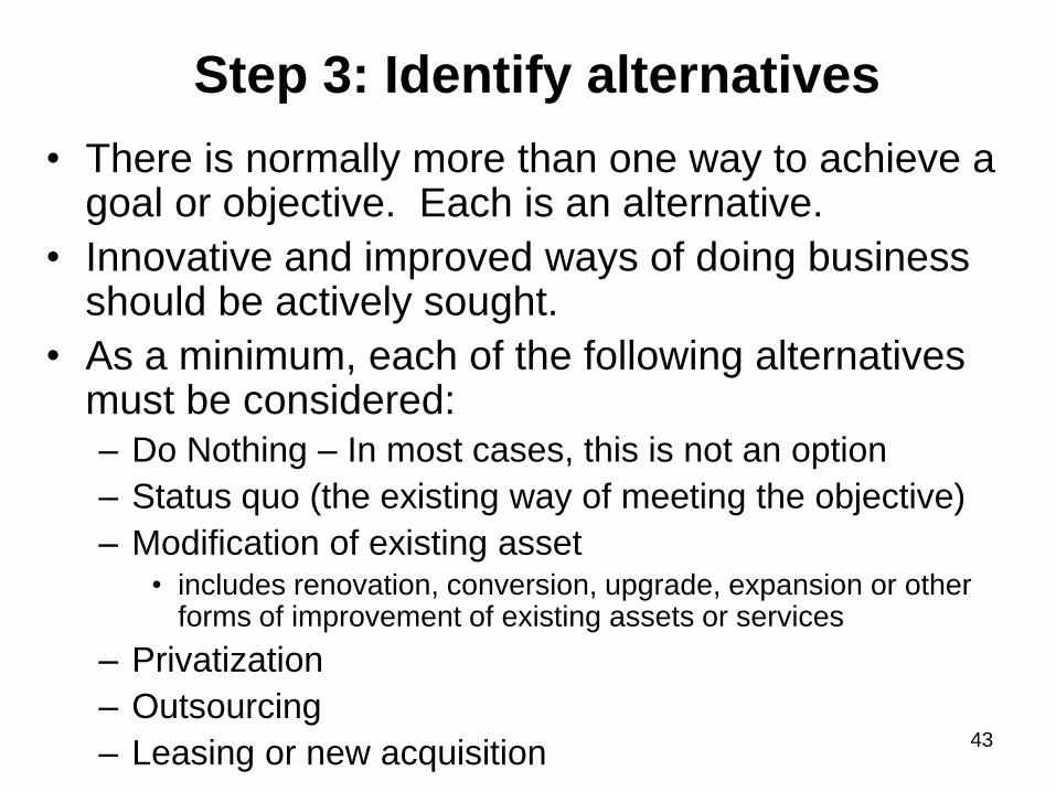
Step 3: Identify alternatives
• There is normally more than one way to achieve a goal or objective. Each is an alternative.
• Innovative and improved ways of doing business should be actively sought.
• As a minimum, each of the following alternatives must be considered: – Do Nothing – In most cases, this is not an option
– Status quo (the existing way of meeting the objective)
– Modification of existing asset • includes renovation, conversion, upgrade, expansion or other
forms of improvement of existing assets or services
– Privatization
– Outsourcing
– Leasing or new acquisition
44
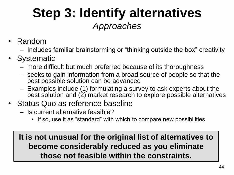
Step 3: Identify alternatives Approaches
• Random – Includes familiar brainstorming or ―thinking outside the box‖ creativity
• Systematic – more difficult but much preferred because of its thoroughness
– seeks to gain information from a broad source of people so that the best possible solution can be advanced
– Examples include (1) formulating a survey to ask experts about the best solution and (2) market research to explore possible alternatives
• Status Quo as reference baseline – Is current alternative feasible?
• If so, use it as ―standard‖ with which to compare new possibilities
It is not unusual for the original list of alternatives to
become considerably reduced as you eliminate
those not feasible within the constraints.

45
Step 3: Identify alternatives Caution on Bias
There are factors in generating alternatives that limit the
range and variety that you develop …
• Inherent biases preventing you from considering certain
aspects or possibilities or
• Resource limitations that force a halt before all concepts
are pursued. Others limiting factors are:
– Routine pressure of normal activities
– Tradeoffs between time and the effort expended and the probability
of new alternatives or additional data
– Precedence of past actions
– Nature of the organization
– Scope of the analysis (feasibility study vs detailed project report)
– Forced deadlines, limiting the analysis time
– Specific lists of alternatives from higher levels of management

46
Step 4: Identify and estimate benefits
Benefits are what government expects to receive for the resources expended; measures utility, effectiveness & performance
Typical Quantifiable Benefits Include: • Reduced Resource Requirements
– Personnel, Training, Maintenance, etc.
• Improved Data Entry – Reduced Staff Time; Reduced error rates
• Improved IT Usage – Storage and Retrieval, Distributed Processing
• Improved Operating Performance – Reduced error rates, better quality & productivity
• Cost Avoidance – Eliminate Future Staff Growth, Need for Equipment

47
Step 4: Identify and estimate benefits Non-Quantifiable Benefits (Intangibles)
• For these situations, you may rank the returns according to some hierarchy of values so that a more rational choice of alternatives can be made.
• If a benefit cannot be quantified, it should be documented and described in the economic analysis.
Non-Quantifiable Benefits Include: • Greater versatility
• Improved decision-making
• Better presentation of information
• Fulfillment of operating requirements
• Improved morale
48
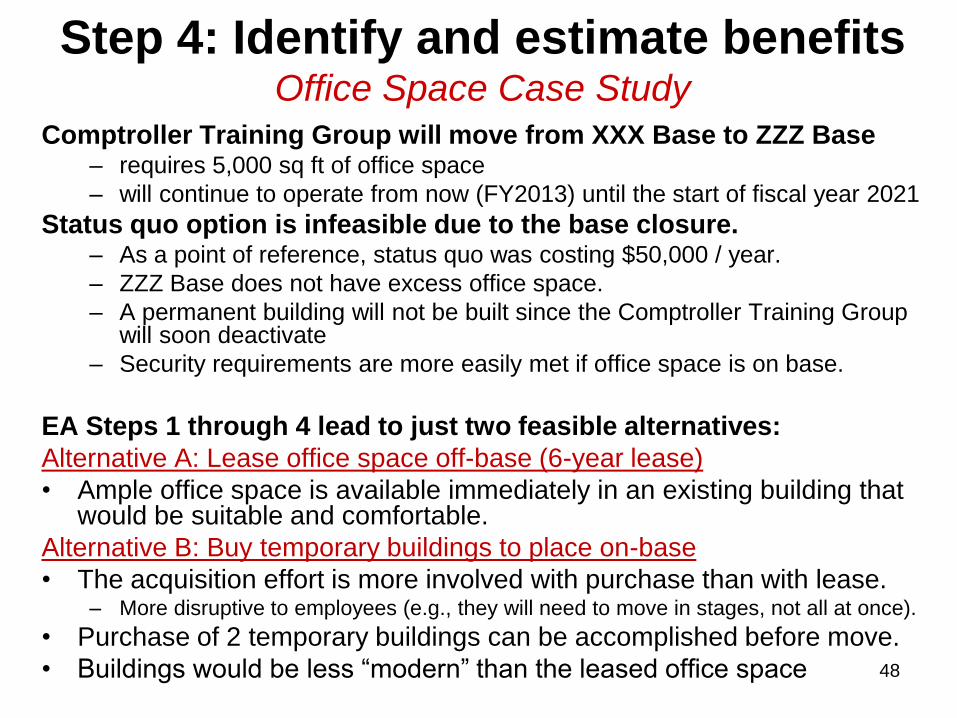
Step 4: Identify and estimate benefits Office Space Case Study
Comptroller Training Group will move from XXX Base to ZZZ Base – requires 5,000 sq ft of office space
– will continue to operate from now (FY2013) until the start of fiscal year 2021
Status quo option is infeasible due to the base closure. – As a point of reference, status quo was costing $50,000 / year.
– ZZZ Base does not have excess office space.
– A permanent building will not be built since the Comptroller Training Group will soon deactivate
– Security requirements are more easily met if office space is on base.
EA Steps 1 through 4 lead to just two feasible alternatives:
Alternative A: Lease office space off-base (6-year lease)
• Ample office space is available immediately in an existing building that would be suitable and comfortable.
Alternative B: Buy temporary buildings to place on-base
• The acquisition effort is more involved with purchase than with lease. – More disruptive to employees (e.g., they will need to move in stages, not all at once).
• Purchase of 2 temporary buildings can be accomplished before move.
• Buildings would be less ―modern‖ than the leased office space
49
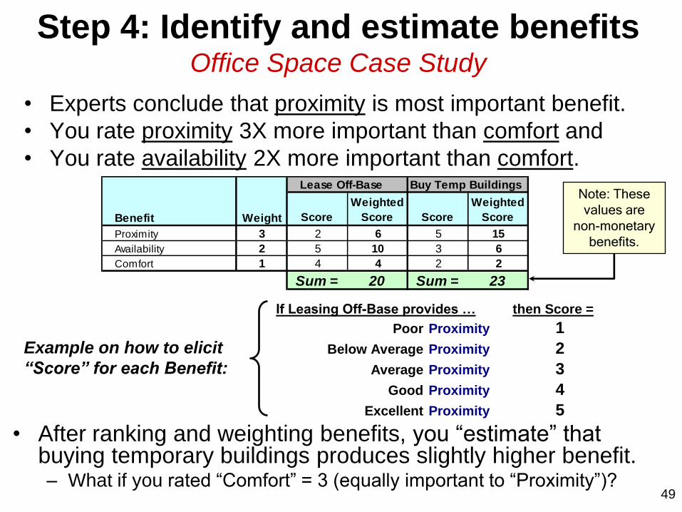
Step 4: Identify and estimate benefits Office Space Case Study
• Experts conclude that proximity is most important benefit.
• You rate proximity 3X more important than comfort and
• You rate availability 2X more important than comfort.
• After ranking and weighting benefits, you ―estimate‖ that buying temporary buildings produces slightly higher benefit. – What if you rated ―Comfort‖ = 3 (equally important to ―Proximity‖)?
If Leasing Off-Base provides … then Score =
Poor Proximity 1
Below Average Proximity 2
Average Proximity 3
Good Proximity 4
Excellent Proximity 5
Example on how to elicit
“Score” for each Benefit:
Lease Off-Base Buy Temp Buildings
Score
Weighted
Score Score
Weighted
Score
Proximity 3 2 6 5 15
Availability 2 5 10 3 6
Comfort 1 4 4 2 2
Sum = 20 Sum = 23
Benefit Weight
Note: These
values are
non-monetary
benefits.

50
Step 4b: Identify and estimate costs Basic Principles
• Viewpoint should reflect total cost to Federal Government – Include budgetary costs to Federal Government
– Include non-budgetary costs to Federal Government • Example: Displacing other government employees, reducing
value of land, need for heightened security, etc.
– Include opportunity costs to Federal Government
– Document the source and derivation of all costs
• Life Cycle Cost – Non-recurring => typically a one-time investment
– Recurring => includes personnel, supplies & matls, M&R
51
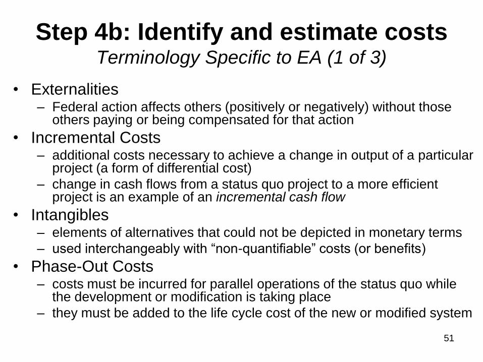
Step 4b: Identify and estimate costs Terminology Specific to EA (1 of 3)
• Externalities – Federal action affects others (positively or negatively) without those
others paying or being compensated for that action
• Incremental Costs – additional costs necessary to achieve a change in output of a particular
project (a form of differential cost)
– change in cash flows from a status quo project to a more efficient project is an example of an incremental cash flow
• Intangibles – elements of alternatives that could not be depicted in monetary terms
– used interchangeably with ―non-quantifiable‖ costs (or benefits)
• Phase-Out Costs – costs must be incurred for parallel operations of the status quo while
the development or modification is taking place
– they must be added to the life cycle cost of the new or modified system

52
Step 4b: Identify and estimate costs Terminology Specific to EA (2 of 3)
• Sunk Costs – costs that have already been incurred or were irrevocably committed
prior to the beginning of the period-of-comparison
– not included in the EA but may be mentioned in the narrative of report
• Terminal Cost – costs that will be incurred due to actions taken to terminate a program
– also referred to as ―residual‖ or ―salvage value‖
• Wash Costs – costs that apply equally to all alternatives
– can be included or excluded in EA
– also referred to as ―non-differential costs‖
• Opportunity Cost – value of a good or service foregone or sacrificed by use of limited
resources on a less effective or less gainful project
53
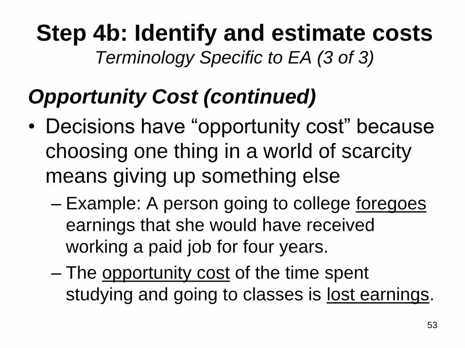
Step 4b: Identify and estimate costs Terminology Specific to EA (3 of 3)
Opportunity Cost (continued)
• Decisions have ―opportunity cost‖ because
choosing one thing in a world of scarcity
means giving up something else
– Example: A person going to college foregoes
earnings that she would have received
working a paid job for four years.
– The opportunity cost of the time spent
studying and going to classes is lost earnings.

54
Step 4b: Identify and estimate costs Treatment of Inflation
Inflation should be recognized in EA by
either of the following methods:
• The first and preferred method is to exclude
inflation by using ―base year dollar‖ (i.e. constant
dollar) estimates.
• The second method is to use ―then-year dollar‖
estimates that include inflation.
We prefer to show costs and benefits in constant dollars.
Therefore, we‟ll apply real (not nominal) discount rates.
55
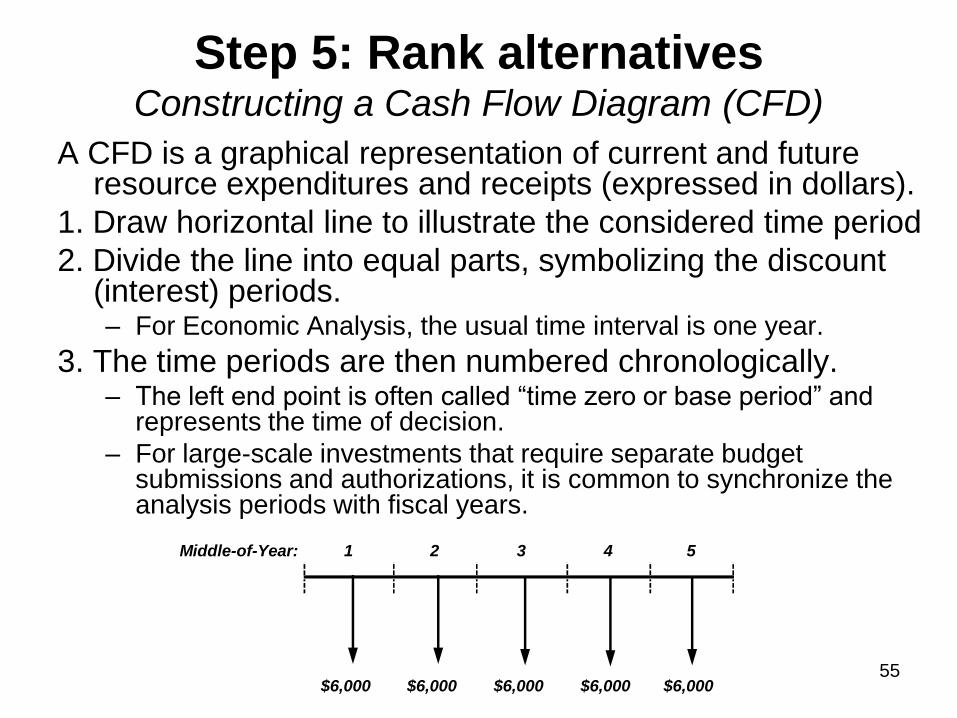
Step 5: Rank alternatives Constructing a Cash Flow Diagram (CFD)
A CFD is a graphical representation of current and future resource expenditures and receipts (expressed in dollars).
1. Draw horizontal line to illustrate the considered time period
2. Divide the line into equal parts, symbolizing the discount (interest) periods. – For Economic Analysis, the usual time interval is one year.
3. The time periods are then numbered chronologically. – The left end point is often called ―time zero or base period‖ and
represents the time of decision.
– For large-scale investments that require separate budget submissions and authorizations, it is common to synchronize the analysis periods with fiscal years.
Middle-of-Year: 1 2 3 4 5
$6,000 $6,000 $6,000 $6,000 $6,000

56
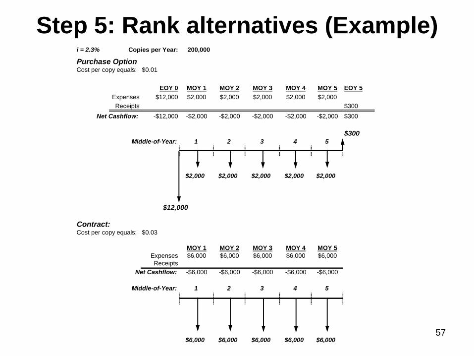
Step 5: Rank alternatives Constructing a CFD (Example)
• An office requires a new copy machine that will
be used to produce 200,000 copies per year.
• Alternative 1 - purchase new copying machine.
– Price = $12,000 that will be paid one month after
delivery. The machine is delivered immediately.
– Operating and maintenance costs = $0.01 per copy
– The copy machine will last for 5 years at which time it
will have a salvage value of $300.
• Alternative 2 is contracted service at a cost of
$0.03 per copy. The discount rate is 2.3 percent.
57
Step 5: Rank alternatives (Example) i = 2.3% Copies per Year: 200,000
Purchase OptionCost per copy equals: $0.01
EOY 0 MOY 1 MOY 2 MOY 3 MOY 4 MOY 5 EOY 5
Expenses $12,000 $2,000 $2,000 $2,000 $2,000 $2,000
Receipts $300
Net Cashflow: -$12,000 -$2,000 -$2,000 -$2,000 -$2,000 -$2,000 $300
$300Middle-of-Year: 1 2 3 4 5
$2,000 $2,000 $2,000 $2,000 $2,000
Contract:Cost per copy equals: $0.03
MOY 1 MOY 2 MOY 3 MOY 4 MOY 5
Expenses $6,000 $6,000 $6,000 $6,000 $6,000
Receipts
Net Cashflow: -$6,000 -$6,000 -$6,000 -$6,000 -$6,000
Middle-of-Year: 1 2 3 4 5
$6,000 $6,000 $6,000 $6,000 $6,000
$12,000
58
Step 5: Rank alternatives Economic Measures-of-Merit (Office Space Case Study)
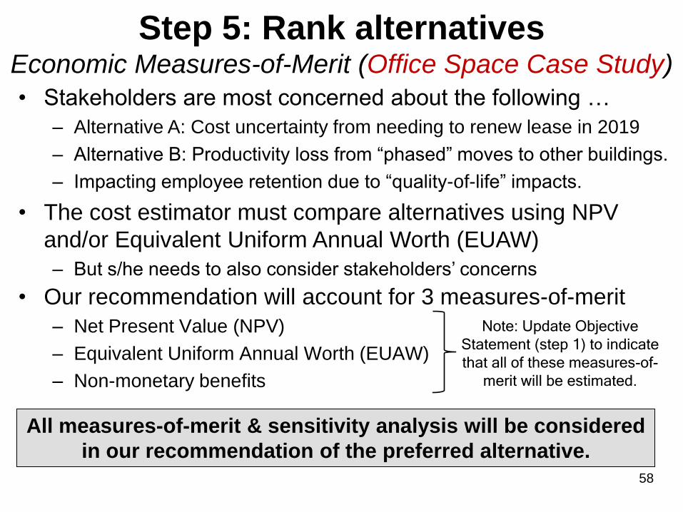
• Our recommendation will account for 3 measures-of-merit
– Net Present Value (NPV)
– Equivalent Uniform Annual Worth (EUAW)
– Non-monetary benefits
• Stakeholders are most concerned about the following …
– Alternative A: Cost uncertainty from needing to renew lease in 2019
– Alternative B: Productivity loss from ―phased‖ moves to other buildings.
– Impacting employee retention due to ―quality-of-life‖ impacts.
• The cost estimator must compare alternatives using NPV
and/or Equivalent Uniform Annual Worth (EUAW)
– But s/he needs to also consider stakeholders‘ concerns
All measures-of-merit & sensitivity analysis will be considered
in our recommendation of the preferred alternative.
Note: Update Objective
Statement (step 1) to indicate
that all of these measures-of-
merit will be estimated.

59
Step 5: Rank alternatives Net Present Value (NPV)
• NPV is the amount of dollars that would have to be invested during the base year at the assumed discount (interest) rate to cover the costs or match the revenues or savings at a specific point in the future. – All costs and benefits reduced to a single discounted net value.
– Enables simple comparison of alternatives on an equitable basis
• The following conditions apply to the present worth method. Note that for these conditions, economic life is assumed to be equal to the period of analysis. – Economic lives of alternatives must be finite. For example, pump
A has been estimated to have a physical life of 6 years. Pump B has an estimated life of 12 years
– Economic lives of alternatives must be equal, or else they must be placed on equal terms.

60
Step 5: Rank alternatives Net Present Value (NPV)
If alternatives have unequal economic lives, then three adjustments are possible:
• Assume multiple procurements are possible for each alternative until both have the same economic life. – Assumes the same value of benefit can be purchased again and again.
– e.g., if two alternatives have economic lives of 6 and 8 years, the common multiple would be 24 years, which might be unrealistic.
• Shorten the economic life of the longer alternative. – e.g., if 2 alternatives have economic lives of 6 and 8 years, use 6 years.
– May result in an increase in terminal value.
• Extend the economic life of the shorter alternative. – e.g., if 2 alternatives have economic lives of 6 and 8 years, force both to
have 8-year economic lives.
– May result in additional costs, increased costs or degradation of benefits.
61
Step 5: Rank alternatives Net Present Value (NPV)
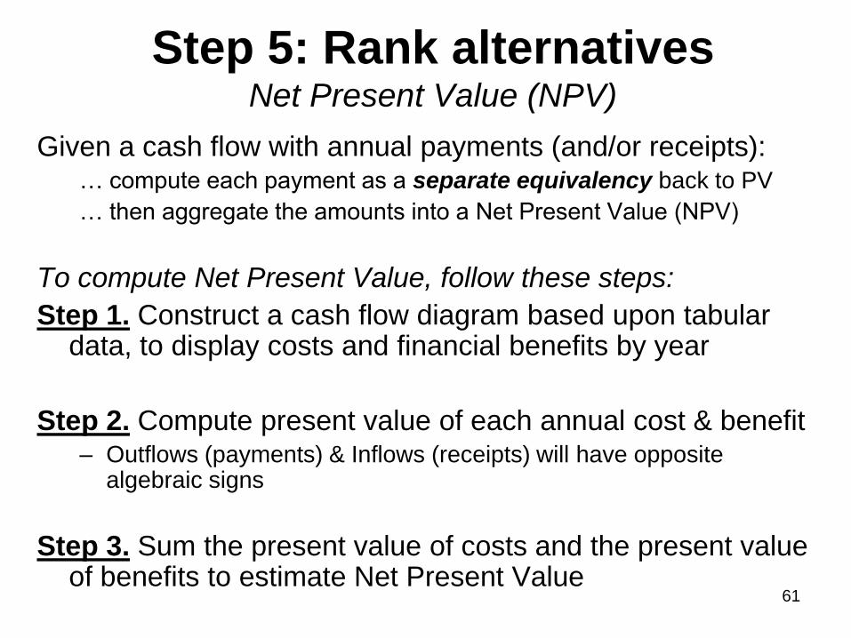
Given a cash flow with annual payments (and/or receipts): … compute each payment as a separate equivalency back to PV
… then aggregate the amounts into a Net Present Value (NPV)
To compute Net Present Value, follow these steps:
Step 1. Construct a cash flow diagram based upon tabular data, to display costs and financial benefits by year
Step 2. Compute present value of each annual cost & benefit – Outflows (payments) & Inflows (receipts) will have opposite
algebraic signs
Step 3. Sum the present value of costs and the present value of benefits to estimate Net Present Value

62
Step 5: Rank alternatives Net Present Value (NPV)
where … n = number of years (i.e. period of analysis)
Benefits = monetized value of positive cash flow in year k
Costs = monetized value of negative cash flow in year k
Example: in year 3: Benefits = 30, Costs = - 50, (Benefits + Costs) = - 20
• Discounting net cash flows transforms gains & losses occurring
in different time periods to common unit of measurement
• Standard criterion for justifying investments on economic
principles NPV > 0.
– The alternative with ‗most positive‘ NPV is typically the most preferred.
Note: If annual Costs are depicted as positive values, then:
Net cash flow at end-of-year k
= Discount factor for year k

63
Step 5: Rank alternatives NPV (Office Space Case Study)
Alternative A. We can lease 5,000 sq ft of office space for $10.00 per sq ft per year for six years beginning 1 Oct 2013 – The owner will pay maintenance and utility costs.
Alternative B. We can buy 2 temporary buildings for $190,000. Each can be delivered and blocked by 1 Oct 2013 at an additional upfront cost of $10,000. – Maintenance and utilities are expected to cost $30,000 per year.
– Each building has an economic life of eight years.
– Civil Engineers predict the buildings can be disposed at the end of eighth year for a net salvage value of $50,000 (this is an inflow)
For both alternatives: Assume period of analysis is equal to the economic life.
– Two different periods of analysis: six years or eight years • The real discount rate for either period of analysis is 2.7%.
64
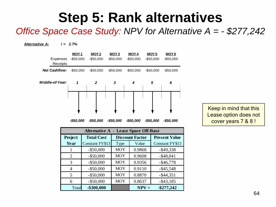
Step 5: Rank alternatives Office Space Case Study: NPV for Alternative A = - $277,242
Total Cost Present Value
Constant FY$13 Type Value Constant FY$13
1 -$50,000 MOY 0.9868 -$49,338
2 -$50,000 MOY 0.9608 -$48,041
3 -$50,000 MOY 0.9356 -$46,778
4 -$50,000 MOY 0.9110 -$45,548
5 -$50,000 MOY 0.8870 -$44,351
6 -$50,000 MOY 0.8637 -$43,185
Total -$300,000 NPV = -$277,242
Alternative A - Lease Space Off-Base
Project
Year
Discount Factor
Keep in mind that this
Lease option does not
cover years 7 & 8 !
Alternative A: i = 2.7%
MOY 1 MOY 2 MOY 3 MOY 4 MOY 5 MOY 6
Expenses -$50,000 -$50,000 -$50,000 -$50,000 -$50,000 -$50,000
Receipts
Net Cashflow: -$50,000 -$50,000 -$50,000 -$50,000 -$50,000 -$50,000
Middle-of-Year: 1 2 3 4 5 6
-$50,000 -$50,000 -$50,000 -$50,000 -$50,000 -$50,000
65
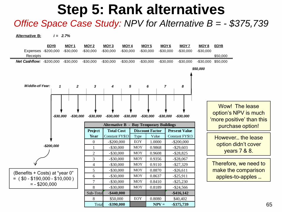
Step 5: Rank alternatives Office Space Case Study: NPV for Alternative B = - $375,739
Wow! The lease
option‟s NPV is much
„more positive‟ than this
purchase option!
However… the lease
option didn‟t cover
years 7 & 8.
Therefore, we need to
make the comparison
apples-to-apples …
Total Cost Present Value
Constant FY$13 Type Value Constant FY$13
0 -$200,000 EOY 1.0000 -$200,000
1 -$30,000 MOY 0.9868 -$29,603
2 -$30,000 MOY 0.9608 -$28,825
3 -$30,000 MOY 0.9356 -$28,067
4 -$30,000 MOY 0.9110 -$27,329
5 -$30,000 MOY 0.8870 -$26,611
6 -$30,000 MOY 0.8637 -$25,911
7 -$30,000 MOY 0.8410 -$25,230
8 -$30,000 MOY 0.8189 -$24,566
Sub-Total -$440,000 -$416,142
8 $50,000 EOY 0.8080 $40,402
Total -$390,000 NPV = -$375,739
Alternative B - Buy Temporary Buildings
Project
Year
Discount Factor
Alternative B: i = 2.7%
EOY0 MOY 1 MOY 2 MOY 3 MOY 4 MOY 5 MOY 6 MOY 7 MOY 8 EOY8
Expenses -$200,000 -$30,000 -$30,000 -$30,000 -$30,000 -$30,000 -$30,000 -$30,000 -$30,000
Receipts $50,000
Net Cashflow: -$200,000 -$30,000 -$30,000 -$30,000 -$30,000 -$30,000 -$30,000 -$30,000 -$30,000 $50,000
$50,000
Middle-of-Year: 1 2 3 4 5 6 7 8
-$30,000 -$30,000 -$30,000 -$30,000 -$30,000 -$30,000 -$30,000 -$30,000
-$200,000
(Benefits + Costs) at “year 0”
= ( $0 - $190,000 - $10,000 )
= - $200,000
66
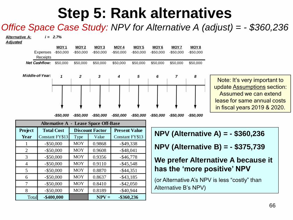
Step 5: Rank alternatives Office Space Case Study: NPV for Alternative A (adjust) = - $360,236
NPV (Alternative A) = - $360,236
NPV (Alternative B) = - $375,739
We prefer Alternative A because it
has the „more positive‟ NPV
(or Alternative A‘s NPV is less ―costly‖ than
Alternative B‘s NPV)
Note: It‟s very important to
update Assumptions section:
Assumed we can extend
lease for same annual costs
in fiscal years 2019 & 2020.
Total Cost Present Value
Constant FY$13 Type Value Constant FY$13
1 -$50,000 MOY 0.9868 -$49,338
2 -$50,000 MOY 0.9608 -$48,041
3 -$50,000 MOY 0.9356 -$46,778
4 -$50,000 MOY 0.9110 -$45,548
5 -$50,000 MOY 0.8870 -$44,351
6 -$50,000 MOY 0.8637 -$43,185
7 -$50,000 MOY 0.8410 -$42,050
8 -$50,000 MOY 0.8189 -$40,944
Total -$400,000 NPV = -$360,236
Alternative A - Lease Space Off-Base
Project
Year
Discount Factor
Alternative A: i = 2.7%
Adjusted
MOY 1 MOY 2 MOY 3 MOY 4 MOY 5 MOY 6 MOY 7 MOY 8
Expenses -$50,000 -$50,000 -$50,000 -$50,000 -$50,000 -$50,000 -$50,000 -$50,000
Receipts
Net Cashflow: $50,000 $50,000 $50,000 $50,000 $50,000 $50,000 $50,000 $50,000
Middle-of-Year: 1 2 3 4 5 6 7 8
-$50,000 -$50,000 -$50,000 -$50,000 -$50,000 -$50,000 -$50,000 -$50,000

67
Step 5: Rank alternatives Equivalent Uniform Annual Worth (EUAW)
• All receipts and expenditures are transformed into an equivalent annual worth over the life of the project or investment. – The NPV is reduced to an ―average dollars per year‖
annual payment (or receipt) that can be compared with that of a competing project
• The alternative with the highest EUAW is the most economical choice – assumes alternatives have equal non-monetary benefits
Useful when alternatives have different economic lives

68
Step 5: Rank alternatives Calculating Equivalent Uniform Annual Worth (EUAW)
Step 1: Compute the NPV of each alternative using present value techniques.
Step 2: Divide the NPV by the sum of the annual discount factors for the years 1 through n
or
Step 2: Multiply the NPV by the Capital Recovery Factor (CRF)
If Cash Flows End-of-Year (EOY) from year 1 through n: If Cash Flows Middle-of-Year (MOY) from year 1 through n:
If Cash Flows End-of-Year
(EOY) from year 1 through n: If Cash Flows Middle-of-Year
(MOY) from year 1 through n:
69
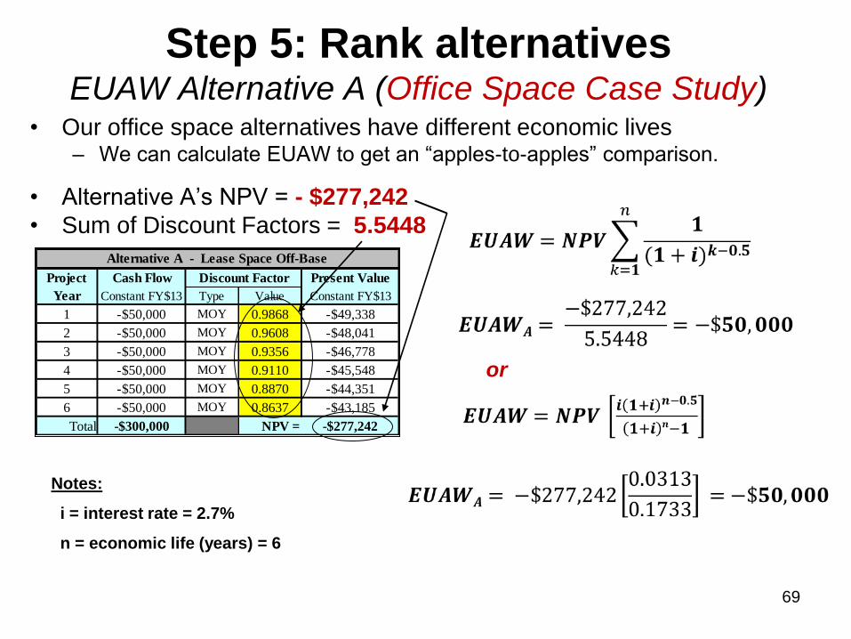
Step 5: Rank alternatives EUAW Alternative A (Office Space Case Study)
• Our office space alternatives have different economic lives – We can calculate EUAW to get an ―apples-to-apples‖ comparison.
• Alternative A‘s NPV = - $277,242
• Sum of Discount Factors = 5.5448
Cash Flow Present Value
Constant FY$13 Type Value Constant FY$13
1 -$50,000 MOY 0.9868 -$49,338
2 -$50,000 MOY 0.9608 -$48,041
3 -$50,000 MOY 0.9356 -$46,778
4 -$50,000 MOY 0.9110 -$45,548
5 -$50,000 MOY 0.8870 -$44,351
6 -$50,000 MOY 0.8637 -$43,185
Total -$300,000 NPV = -$277,242
Alternative A - Lease Space Off-Base
Project
Year
Discount Factor
or
Notes:
i = interest rate = 2.7%
n = economic life (years) = 6

70
Step 5: Rank alternatives EUAW Alternative B (Office Space Case Study)
• For EOY Cash Flows, NPV = -$200,000 + $40,402 = - $159,598
• For MOY Cash Flows, NPV = -$416,142 + $200,000 = - $216,142
• Total EUAW: Total Cost Present Value
Constant FY$13 Type Value Constant FY$13
0 -$200,000 EOY 1.0000 -$200,000
1 -$30,000 MOY 0.9868 -$29,603
2 -$30,000 MOY 0.9608 -$28,825
3 -$30,000 MOY 0.9356 -$28,067
4 -$30,000 MOY 0.9110 -$27,329
5 -$30,000 MOY 0.8870 -$26,611
6 -$30,000 MOY 0.8637 -$25,911
7 -$30,000 MOY 0.8410 -$25,230
8 -$30,000 MOY 0.8189 -$24,566
Sub-Total -$440,000 -$416,142
8 $50,000 EOY 0.8080 $40,402
Total -$390,000 NPV = -$375,739
Discount Factor
Alternative B - Buy Temporary Buildings
Project
Year
Notes:
i = interest rate = 2.7%
n = economic life (years) = 8
71
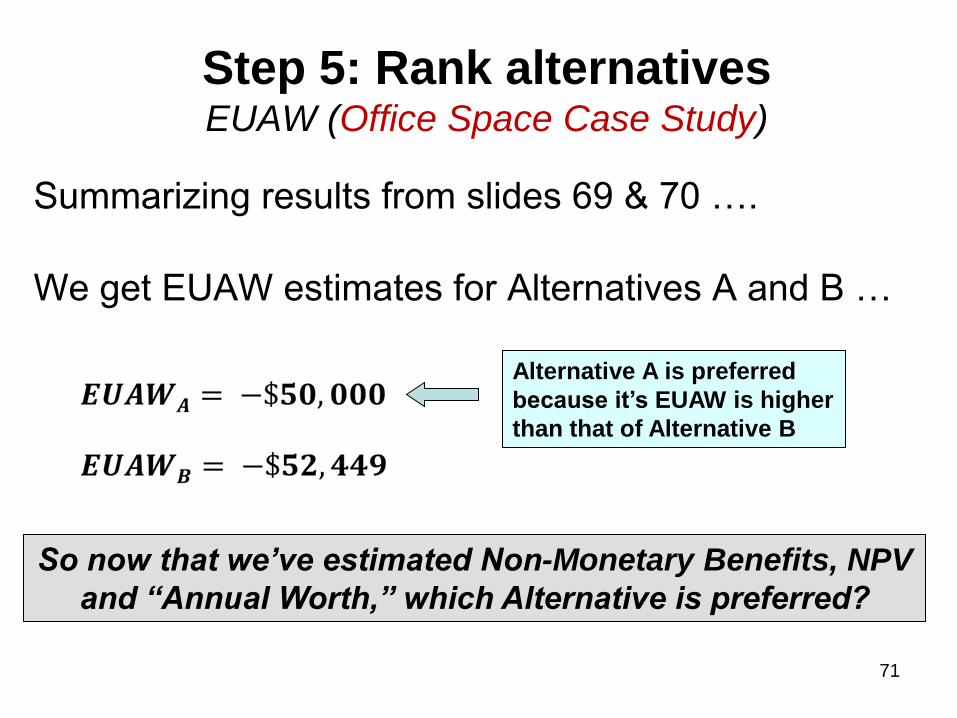
Step 5: Rank alternatives EUAW (Office Space Case Study)
Summarizing results from slides 69 & 70 ….
We get EUAW estimates for Alternatives A and B …
Alternative A is preferred
because it‟s EUAW is higher
than that of Alternative B
So now that we’ve estimated Non-Monetary Benefits, NPV
and “Annual Worth,” which Alternative is preferred?

72
Step 5: Rank alternatives Considering All Economic Measures-of-Merit
• Decision-makers tend to have preferences for specific financial measures – because of personal experience, program constraints,
or expectations from senior leadership.
• For example, some programs place more emphasis on the magnitude of NPV while others would prefer to see a short payback period
• Therefore, estimating several measures-of-merit will help both analysts and decision-makers in gaining more insight into the ―relative worth‖ of each feasible alternative.

73
Step 5: Rank alternatives Considering All Economic Measures-of-Merit for the
Office Space Case Study (Preliminary)
Although Alternative B produces more Benefit, we had a slight
preference to Alternative A based on its higher NPV and EUAW.
Alternative
A
Alternative
B
Lease Buy Temp
Off-Base Buildings Lease Off-
Base
Buy Temp
Buildings
Non-Monetary Units of Benefit 20.00 23.00
Net Present Value (NPV) -$360,236 -$375,739
Equivalent Uniform Annual Worth (EUAW) -$50,000 -$52,152
# Selected 2 1
Recommend
Measure-of-Merit (MoM)
Preferred Alternative

74
Step 6: Perform sensitivity analysis
• An EA sensitivity analysis is a "what-if" exercise
– It tests whether the conclusion of an EA will change if
a benefit, cost, or other assumed variable changes.
• An EA sensitivity analysis should be performed
when
– The results of the economic analysis do not clearly
favor any one alternative, or
– There is uncertainty about an assumption that can
impact the estimate of costs and benefits in the
economic analysis.
75
Step 6: Perform sensitivity analysis
• Sensitivity analysis enables you to study how a variable or assumption impacts the recommendation
• Discount rate plays key role in ranking of alternatives
• A common analysis is to measure the relative values of alternatives after varying discount rates.
• Some input variables subject to sensitivity analysis: – costs or reimbursements
– performance output or benefits
– system lives or economic life
– estimating of operation-support-maintenance factors
– schedules
– other risk or unknown aspects
76
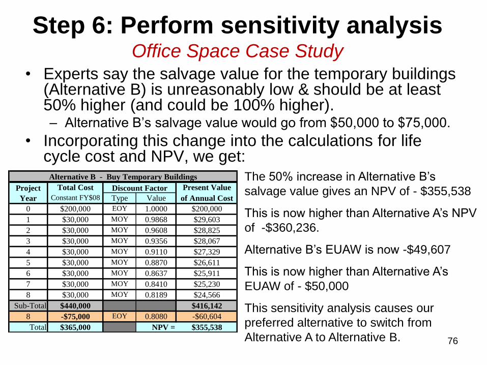
Step 6: Perform sensitivity analysis Office Space Case Study
• Experts say the salvage value for the temporary buildings (Alternative B) is unreasonably low & should be at least 50% higher (and could be 100% higher). – Alternative B‘s salvage value would go from $50,000 to $75,000.
• Incorporating this change into the calculations for life cycle cost and NPV, we get:
Total Cost Present Value
Constant FY$08 Type Value of Annual Cost
0 $200,000 EOY 1.0000 $200,000
1 $30,000 MOY 0.9868 $29,603
2 $30,000 MOY 0.9608 $28,825
3 $30,000 MOY 0.9356 $28,067
4 $30,000 MOY 0.9110 $27,329
5 $30,000 MOY 0.8870 $26,611
6 $30,000 MOY 0.8637 $25,911
7 $30,000 MOY 0.8410 $25,230
8 $30,000 MOY 0.8189 $24,566
Sub-Total $440,000 $416,142
8 -$75,000 EOY 0.8080 -$60,604
Total $365,000 NPV = $355,538
Discount Factor
Alternative B - Buy Temporary Buildings
Project
Year
The 50% increase in Alternative B‘s
salvage value gives an NPV of - $355,538
This is now higher than Alternative A‘s NPV
of -$360,236.
Alternative B‘s EUAW is now -$49,607
This is now higher than Alternative A‘s
EUAW of - $50,000
This sensitivity analysis causes our
preferred alternative to switch from
Alternative A to Alternative B.

77
Step 5: Rank alternatives Considering All Economic Measures-of-Merit for the
Office Space Case Study (Final)
It is important to frequently revisit all assumptions that
affect each measure-of-merit.
Alternative
A
Alternative
B
Lease Buy Temp
Off-Base Buildings Lease Off-
Base
Buy Temp
Buildings
Non-Monetary Units of Benefit 20.00 23.00
Net Present Value (NPV) -$360,236 -$355,538
Equivalent Uniform Annual Worth (EUAW) -$50,000 -$49,348
# Selected 0 3
Recommend
Measure-of-Merit (MoM)
Preferred Alternative
78
Step 7: Prepare results
• Executive Summary
– refer to benefits and costs of the alternatives
– interpret results to include a recommendation of the preferred alternative.
• Body of report
– The completed analysis must be structured to facilitate understanding on the part of the decision-maker
– include all sources of data and calculations (auditable)

79
Step 7: Make recommendation
• The analyst has two courses of action:
– Present the alternatives in a listing or ranking from
which the ultimate course of action can be selected or
– Make a firm recommendation for the manager‘s
consideration.
• The actual decision will be based on quantitative
factors, as well as qualitative factors, such as the
judgment and experience of the decision maker
80
Summary • We defined an economic analysis (EA)
• We explained why discounting calculations are performed
• We showed how discount factors are calculated – End-of-Year (EOY) and Middle-of-Year (MOY) conventions
• We discussed the steps of an EA
• We demonstrated the steps of an EA (using examples)
• We developed cash flow diagrams for feasible alternatives
• We applied discount factors to cash flows
• We calculated EA measures-of-merit such as: – Net Present Value (NPV)
– Equivalent Uniform Annual Worth (EUAW)
– Non-monetary Benefits
• We discussed sensitivity analysis & provided an example
• We discussed how to recommend the most preferred alternative & provided an example – gives the decision maker tools to make a more informed decision

81
Other Potential Considerations in an EA
• Non-Discounted Measures – Upfront Investment cost
– Total life cycle cost
– ―Return-on-Investment‖ (ROI)
– Payback Period
• Discounted Measures – Internal Rate of Return (IRR)
– Benefit-to-Cost Ratio (BCR)
– Savings-Investment Ratio (SIR)
– Discounted Payback Period
• Combine alternatives that are not mutually exclusive
• Brainstorm opportunity costs
• Interview experts on „intangible‟ benefits & costs

82
BACKUPS
Backup slides

83
H.R.1585
National Defense Authorization Act for
Fiscal Year 2008 (Introduced in House)
SEC. 256. COST-BENEFIT ANALYSIS OF PROPOSED FUNDING REDUCTION FOR HIGH ENERGY LASER SYSTEMS TEST FACILITY.
(a) Report Required.--Not later than 90 days after the date of the enactment of this Act, the Secretary of Defense shall submit to the congressional defense committees a report containing a cost-benefit analysis of the proposed reduction in Army research, development, test, and evaluation funding for the High Energy Laser Systems Test Facility.
Legislative Record U.S. Senate 1 October 2007
84
Federal & DoD Guidance Federal
• OMB Circular A-94: Guidelines and Discount Rates for Benefit-Cost Analysis of Federal Programs. – serves as the overall reference for all DoD and non-DoD programs.
– important data from this document are the discount rates (similar to interest rates) that OMB updates annually.
DoD
• DoDI 7000.14R: Financial Management Regulations. – Provides cost-benefit guidance, typically used for evaluating
Defense Working Capital Fund scenarios
• DoDI 7041.3 – Provides general EA guidance to support investment
Air Force
• AFPD 65-5 (17 May 93), Cost and Economics,
• AFI 65-501 (10 Nov 04), Economic Analysis Instruction and
• AFMAN 65-506 (10 Nov 04), Economic Analysis Manual

85
When an EA is Required: OMB
DoD Instructions 7041.3 and 7000.14R require
that the economic analysis methodology be
applied to all considerations of investment.

86
When an EA is Required: DoD
DoD Instructions 7041.3 and 7000.14R require
that the economic analysis methodology be
applied to all considerations of investment.
DoDI 7041.3, section 3.2 (Policy):
• “procedures … at a minimum, must be followed
by the DoD Components in economic analyses
submitted to the Under Secretary of Defense
(Comptroller) to support budget line items
exceeding the investment-expense criteria of
DoD 7000.14-R.”

87
When an EA is Required: USAF
AFI 65-501: Economic Analysis Instruction
• EA required when ―deciding whether to commit resources to a new project of program with total investment costs over $1,000,000 or annual recurring costs over $250,000 for at least 4 years
• Other criteria that warrant an EA include cases when: – proposing housing or utilities privatization project, regardless of
investment cost
– a functional user or program office is procuring, modernizing or upgrading a material solution for various types of Information Systems that are not designated to support the Clinger-Cohen Act
– Secretariat or Air Staff of a commander of field units direct an EA study

88
When an EA is Not Required
There are cases, however, when instructions or
directives can waive an EA. Such exceptions
include the following initiatives:
– Environmental or hazardous waste reduction,
– OSD or higher authority directs a new or modified
program & specifies how to accomplish program goals,
– Congress mandates the alternative that must be taken,
– Legislation specifies that the project is exempt from
requiring an EA, and
– If the cost of doing EA analysis outweighs the potential
benefits of the information output from the EA

89
Interest Rate (Example) • A mortgage company lends you $300,000 at a 6%
annual fixed interest rate; you agree to pay off the loan (by month) over 30 years
• The mortgage company has charged you a premium for use of the loan = 6% interest rate
• If there was no premium, you would pay the mortgage company $10,000 a year for 30-years and there would be a zero balance at the end of year 30
• Instead, you will pay $21,584 per year for 30 years – A ―premium‖ of $11,584 per year over the life of the loan
– Assuming the absence of inflation, your difference in payment reflects the real annual cost of borrowing money (and the lender‘s annual real benefit of lending money)

90
Simple Interest Formula
I = total interest earned or paid
PV = present value; principal amount lent or borrowed
n = number of interest periods (e.g. years)
i = interest rate per interest period
( )( )( ) I PV n i
If PV were a loan, the total amount repaid at the end of n periods, also known as ―Future Value (FV) = PV + I
Substituting I with (PV)(n)(i), FV = PV + (PV)(n)(i).
Therefore, FV simplifies to:
(1 ) FV PV n i

91
Discount Factor Formula Based on MOY Convention
PV = FV * MOY Discount Factor
0.5
1
(1 )nPV FV
i
Substituting, we get …
Present Value formula for MOY Payments:
We define …
0.5
1=MOY Discount Factor
(1 )ni
92
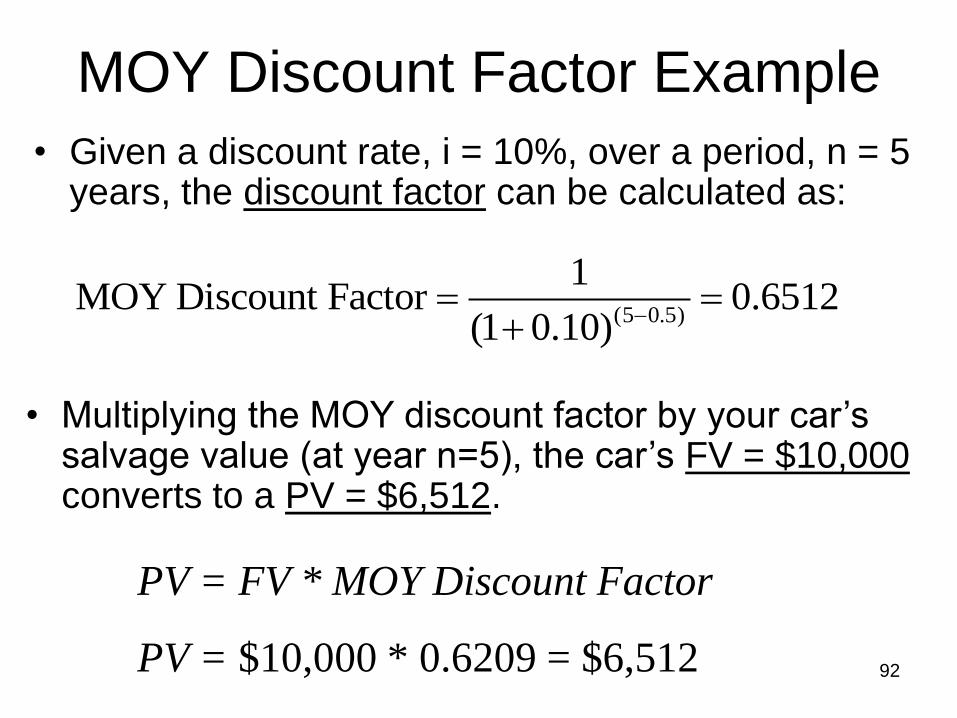
MOY Discount Factor Example
• Given a discount rate, i = 10%, over a period, n = 5 years, the discount factor can be calculated as:
PV = FV * MOY Discount Factor
PV = $10,000 * 0.6209 = $6,512
• Multiplying the MOY discount factor by your car‘s salvage value (at year n=5), the car‘s FV = $10,000 converts to a PV = $6,512.
(5 0.5)
1MOY Discount Factor 0.6512
(1 0.10)
93
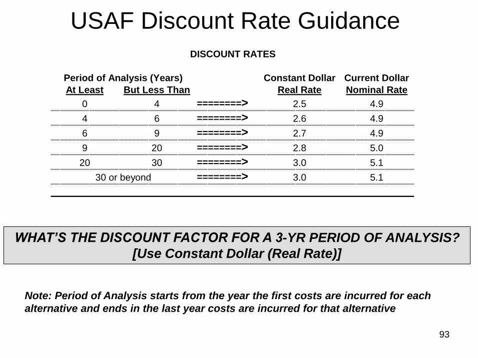
USAF Discount Rate Guidance
WHAT’S THE DISCOUNT FACTOR FOR A 3-YR PERIOD OF ANALYSIS?
[Use Constant Dollar (Real Rate)]
Note: Period of Analysis starts from the year the first costs are incurred for each
alternative and ends in the last year costs are incurred for that alternative
Constant Dollar Current Dollar
At Least But Less Than Real Rate Nominal Rate
0 4 ========> 2.5 4.9
4 6 ========> 2.6 4.9
6 9 ========> 2.7 4.9
9 20 ========> 2.8 5.0
20 30 ========> 3.0 5.1
========> 3.0 5.130 or beyond
DISCOUNT RATES
Period of Analysis (Years)

94
Step 2a: List assumptions
State-of-Nature and Mathematical
• State-of-Nature Assumptions. – determine the limits of the analysis and permit the analyst to
construct alternatives.
– Examples: • Mission requirements will remain unchanged for 20 years.
• Our agency will continue to be active for 30 years after the project
• Mathematical – involve calculating procedures used to measure amounts of
resources and benefits.
– Examples: • discount rates & tables
• models used to estimate manning levels
• parametric analysis used to estimate future resource and benefits
– Note: sometimes not listed in the assumption section but in source and derivation of costs and benefits.

95
Step 3: Identify alternatives
Determining Reasonableness
• Should be consistent assumptions and constraints
• Should adhere to regulations & legal requirements
• Adequacy
– the capacity of the potential alternative to meet the
actual scope or objective.
• Economically feasibility
– must be compatible with funding realities.
• Ensure all alternatives consider the same mission
– Step 5 will measure differences in acceptability or
effectiveness

96
Step 3: Identify alternatives Final Note
• Inherent bias occurs for continuing traditional method. – You need to develop and evaluate all feasible alternative solutions to
the problem
– Alternatives with the greatest chance of fulfilling the objective will be presented to the decision maker
• Alternative courses of action and their feasibilities should be identified
• Practical limit to the number of alternatives selected for further analysis. – If there are a large number of alternatives, group the alternatives into
similar approaches or do the analysis in steps or levels.
– A best practice is to limit the number of alternatives in a level to no more than five to nine.

97
Step 5: Rank alternatives Uniform Annual Cost (UAC)
• Represents a constant amount which, if paid annually
throughout the economic life of an alternative, would yield
a total discounted project cost equal to the actual present
value cost of the alternative.
• UACs of alternatives are directly comparable because
they represent annual cost.
• More simply put, it gives you some idea which alternative
is a more efficient use of scarce resources.
Alternative 1 UAC = $91K
Alternative 2 UAC = $92K 97
All things being equal, which Alternative do you prefer?

98
Step 5: Rank alternatives How to Calculate Uniform Annual Cost (UAC)
Step 1: Compute the NPV of an alternative using present value techniques. This can be calculated by estimating the total discounted project cost less the discounted salvage value.
Step 2: Divide the NPV by the cumulative present value factor found by summing the annual discount factors for the benefit years (the years associated with economic life)
Total Discounted Project Cost - Discount ed Salvage Value UAC =
Sum of Discount Factors for Benefit Years
where Benefit Years = Economic Life or the O&S Period
equal
to NPV

99
BUY NEW CAR
YEAR R&D INVEST-MENTO&S (assume
.37/mi for 15000 mi) TOTAL COST
DISCOUNT
FACTORS (Period
at least 4 & <6yrs)
PRESENT
VALUE
2000 5,550
2001 5,550
2002 5,550
2003 5,550
2004 5,550
The total project cost, discounted is:
Assume Salvage Value (trade-in value): $4,000
Uniform Annual Cost = (total discounted project cost - discounted salvage value)/(sum of discount factors for benefit yrs)
Uniform Annual Cost =
x 0.8259 3,304
20,000 25,550
5,550
5,550
5,550
5,550
47,750
0.9625
0.9263
0.8916
0.8581
0.8259
4.4644
24,592
5,141
4,948
4,763
4,584
44,027 44,027 20,000 27,750
44,027-3,304
4.4644 =$9,122
0 Total
Step 5: Rank alternatives Example: Buy New Car or Lease New Car

100
Step 5: Rank alternatives Example: Buy New Car or Lease New Car (continued)
LEASE NEW CAR
YEAR R&D
INVEST-
MENT
O&S (assume
.37/mi for
15000 mi)
TOTAL
COST
DISCOUNT
FACTORS (Period < 4yrs)
PRESENT
VALUE
2000 5,550
2001 5,550
2002 5,550
The total project cost, discounted is:
Assume Salvage Value (trade-in value): $0
Uniform Annual Cost = (total discounted project cost - salvage value)/(sum of discount factors for benefit yrs)
Uniform Annual Cost =
3,600
3,600
3,600
9,150
9,150
9,150
0.9634
0.9281
0.8941
2.7856
8,815
8,492
8,181
25,488
25,488
25,488
2.7856 =$9,150
100
Total

101
Step 5: Rank alternatives Evaluating Alternatives based on Benefits & Costs
Possible conditions regarding the benefits and costs of alternatives …
• Both benefits and costs are equal. – A subjective choice may be made
• Benefits are equal; costs are unequal. – Select alternative with preferred economic measures
• Benefits are unequal; costs are equal – Select alternative with best benefit measures
• Both benefits and costs are unequal – Select alternative with best mix of economic and benefit measures

102
Step 5: Rank alternatives Savings/Investment Ratio (SIR)
• When computing an SIR, however, the analyst is not interested in total operations cost — only the difference between the two possibilities. – That is, what effect will the investment have on the operation?
• To calculate the SIR, divide the present value of the savings by the present value of the incremental investment. It can also be calculated by dividing the UAC of savings by the UAC of investment.
Savings
Investment
PVSIR
PV
Savings
Investment
UACSIR
UACor
We‘ll calculate SIR this way

103
Step 5: Rank alternatives (SIR Example)
• Current process (status quo) employs equipment having a market value of $35,000 and results in annual operating costs of $88,000
• Proposed process would employ new (replacement) equipment for a price of $230,000 and results in annual operating costs of $23,000/year.
• The process will be used for the next 8 years. Salvage value will be zero.
• Using a discount rate of 2.5%, what is the SIR?
• Which process do you recommend based on SIR?

104
Step 5: Rank alternatives (SIR Example)
The investment equals the cost of the proposed new equipment ($230,000) less the market value of the equipment currently being used ($35,000):
Investment = $230,000 - $35,000 = $195,000
Annual savings would equal operating costs using existing equipment ($88,000) less the operating costs using to the new equipment ($23,000):
Annual Savings = $88,000-$23,000 = $65,000

105
Step 5: Rank alternatives (SIR Example) Status Quo (SQ) EOY 0 MOY 1 MOY 2 MOY 3 MOY 4 MOY 5 MOY 6 MOY 7 MOY 8 Sum
Expenses $88,000 $88,000 $88,000 $88,000 $88,000 $88,000 $88,000 $88,000 $704,000
Receipts $35,000 $35,000
Net Cashflow: $35,000 -$88,000 -$88,000 -$88,000 -$88,000 -$88,000 -$88,000 -$88,000 -$88,000 -$669,000
Middle-of-Year: 1 2 3 4 5 6 7 8
$35,000
$88,000 $88,000 $88,000 $88,000 $88,000 $88,000 $88,000 $88,000
Alternative (ALT) EOY 0 MOY 1 MOY 2 MOY 3 MOY 4 MOY 5 MOY 6 MOY 7 MOY 8 Sum
Expenses $230,000 $23,000 $23,000 $23,000 $23,000 $23,000 $23,000 $23,000 $23,000 $414,000
Receipts $0
Net Cashflow: -$230,000 -$23,000 -$23,000 -$23,000 -$23,000 -$23,000 -$23,000 -$23,000 -$23,000 -$414,000
Middle-of-Year: 1 2 3 4 5 6 7 8
$23,000 $23,000 $23,000 $23,000 $23,000 $23,000 $23,000 $23,000
$230,000

106
Step 5: Rank alternatives (SIR Example) Incremental Cash Flow
ALT vs. SQ EOY 0 MOY 1 MOY 2 MOY 3 MOY 4 MOY 5 MOY 6 MOY 7 MOY 8 Sum
Net Cashflow: -$195,000 $65,000 $65,000 $65,000 $65,000 $65,000 $65,000 $65,000 $65,000 $325,000
MOY Discount Factor at 2.5%:1
1.0000 0.9877 0.9636 0.9401 0.9172 0.8948 0.8730 0.8517 0.8309
PV of investment (i): $195,000 $195,000
PV of savings (s) $64,202 $62,637 $61,109 $59,618 $58,164 $56,746 $55,362 $54,011 $471,849
SIR = S PV s / S PV i 2.4197
1: MOY Discount Factor Formula = 1/(1+i)^(n-0.5)
$65,000 $65,000 $65,000 $65,000 $65,000 $65,000 $65,000 $65,000
Middle-of-Year: 1 2 3 4 5 6 7 8
$195,000

107
Step 5: Rank alternatives (SIR Example)
$471,8492.42
$195,000
Savings
Investment
PVSIR
PV
• The resultant cash flow reveals that the PV of the investment equals $195,000 because it occurs at time 0 (immediately).
• The PV of savings is the PV of each of eight net ―annual savings‖ of $65,000 (years 1 through 8).
• The total of these present values (PV) equals a PV of savings (sum of PVs) of $471,849.
• Replacing these present value totals into the SIR formula, we get …
• Because the SIR is greater than +1.0 (positive savings and positive investment), we can conclude that the investing in the proposed new equipment is favored over the status quo.