1

Advanced Distribution and Control for Hybrid Intelligent Power Systems Interim Technical Report – Draft – September 17, 2010 Michael Lemmon, Dept. of Electrical Engineering, University of Notre Dame Agreement No. OT-UWM-11012009-03 Prime Contract No. W9132T-10-C-0008 Abstract: This technical report documents Notre Dame’s simPower simulation model of a distributed control and management system for military microgrids. The control/management system uses power inverters to connect a variety of distributed generation sources to the microgrid. Multi-unit stability is assured through the use of a decentralized control system that mimics the P-frequency and Q-voltage droop control used for synchronous machines. Optimal management of this system is accomplished through the use of a novel distributed peer-to-peer algorithm. This distributed optimization algorithm solves the optimal power flow problem in a distributed manner, relying only on local communication between generators on the microgrid. A novel event-triggered message-passing scheme is used to reduce the communication bandwidth used by this algorithm, thereby reducing the cost of communication infrastructure and potentially improving communication security. The work documented in this report was performed between July 1st and September 1st 2010. During this period, a preliminary simPower simulation was built and tested. This simulation models a microgrid proposed by the University of Wisconsin, Madison. Initial testing verified that the decentralized power inverter controls worked as predicted. During this period, the event-triggered generation dispatch algorithm was designed and tested on a simplified microgrid model. Simulations of the proposed dispatch algorithm worked as expected by minimizing the system’s operating costs while simultaneously reducing the amount of message passing in the communication network.

2

Table of Contents: Chapter 1 Introduction 3-4 Chapter 2 Distributed Power Dispatch in Microgrids 5-10 Chapter 3 Event-triggered Power Dispatch 11-13 Chapter 4 Event-triggered Dispatch Simulation Results 14-15 Chapter 5 Microgrid Simulation Development 16-23 Chapter 6 Conclusion

References 24 25

List of Figures: Figure 1 3-bus microgrid with attached agents 10 Figure 2 3-bus microgrid used in event-triggered simulations 14 Figure 3 Simulation result showing time history of generator power 14 Figure 4 Simulation result plotting the time since last broadcast for

event-triggered simulation 14

Figure 5 Top-level simPower model for 3-bus mesh microgrid used in event-triggered dispatch

15

Figure 6 Generator simPower model for event-triggered simulation 15 Figure 7 UWM controller logic (simulink model) 15 Figure 8 UWM Mesh Microgrid 17 Figure 9 Notre Dame simPower model of UWM mesh microgrid 19 Figure 10 Idealized Microsource Generator (simPower) 20 Figure 11 simPower model of ideal microsource generator with UWM

power inverter control component 20

Figure 12 Simulink model of UWM power inverter controller 21 Figure 13 simPower model of diesel generator with synchronous machine

using UWM power inverter component 21

Figure 14 simPower model of external storage device controlled by UWM power inverter

22

Figure 15 simPower model of battery 22 Figure 16 Main grid current time history 23 Figure 17 Bus 2 current and power 23 Figure 18 Distributed generator power delivered 24 Figure 19 Load bus voltages and frequency 24

3

Chapter 1: Introduction

1.1 Background Microgrids [1] are generation/distribution systems in which generation is relatively close to the loads. They can provide a higher level of local resilience to variations in the main power grid’s power quality. This means that microgrids are useful in applications where power reliability is a critical concern. Examples of such applications include hospitals, industrial parks, as well as forward military bases. Microgrids therefore play an important role in maintaining this nation’s military readiness. Decentralized PQ control of distributed generation in microgrids has been previously demonstrated to maintain power quality during islanding and reconnection of the microgrid [2,3]. The equilibrium power levels achieved by these controllers, however, are not necessarily optimal from the standpoint of minimizing overall operating cost. Optimal generation dispatch may be realized through centralized supervision of the entire microgrid. But this approach will be difficult to maintain as the system grows and is therefore not seen as a scalable approach to microgrid energy management. In particular, for applications where the microgrid is expected to evolve over time, one needs to develop an approach to the management of microgrid generation that can quickly adapt to changes in system topology and application mission. The approach being used to meet this need involves the distribution of dispatch and load-shedding decisions across the network [4]. In other words, rather than using a centralized top-down command structure, this project is proposing a distributed bottom-up approach in which computational agents located at the distributed generation source or load bus make local decisions conditioned on information received from neighboring agents. This networked approach to decision-making scales well with system size since the configuration data regarding the grid is stored in a distributed manner. It also provides greater security and resilience to abrupt changes in application mission or grid topology since decision-making and grid configuration data are not handled in a centralized manner. The problem addressed in this project is the development and simulation of a scalable distributed scheme for dispatch and load management in military microgrids. This work is being done as part of a DoD phase II STTR project (Prime Contract No. W9132T-10-C-0008). The University of Notre Dame (technical contact: Michael Lemmon), as a subcontractor to the University of Wisconsin – Madison and Odyssian Technology, is performing this work. The technologies being developed under this project are intended for use in managing electrical generation and loads within microgrids used by military bases.

4

1.2 Objective

The objectives of this project are to

• Develop a simulation of a three-phase microgrid that has been specified by the University of Wisconsin – Madison.

• Developed distributed algorithms for the dispatch of power and intelligent shedding of loads.

• Assist the prime contractor (Odyssian Technology) in the development of embedded software implementing the dispatch and load shedding algorithms.

• Assist the prime contractor (Odyssian Technology) in developing a wireless communication for implementing the proposed algorithms.

The remainder of this report is organized as follows. Chapter 2 discusses the distributed dispatch algorithms being developed under this project. Chapter 3 discusses the development of an event-triggered approach to distributed dispatch that can greatly reduce the amount of communication needed by this approach. Chapter 4 discusses simulation results for a simplified mesh microgrid using the event-triggered dispatch algorithm. Chapter 5 documents on-going work to build a simPower simulation of a mesh microgrid specified by the University of Wisconsin Madison. Chapter 6 reviews project achievements.

5

Chapter 2: Distributed Power Dispatch in Microgrids The power system is modeled as a directed graph, G=(V,E) where V={v1,v2, … ,vN} is a set of nodes representing the system buses, E⊆V×V, is a set of directed edges, representing the power distribution lines. An edge from node I to node j is denoted as eij=(ve,vj) with impedance zij=rij+jxjj. We assume that the line resistance rij is negligible compared to the reactances xij. Let I denote the incidence matrix of the graph G and let D be a diagonal matrix whose entries are the reactances of the distribution lines. We let A=DI denote the weighted incidence matrix of the graph G. The set of neighbors of node i is denoted as N(i) and the set of distribution lines leaving node i is denoted as L(i). Let Sij=Pij+jQij denote the complex power flow from node i to node j, and ui denotes the generator voltage at node i. This voltage is represented in phasor form as ui=|ui|exp(jθj). Under normal operating condition voltages the bus voltages are about equal. In a similar manner, the bus phases are about equal so that the phase difference, θi-θj , is typically small. In this case, the flow of active and reactive power are decoupled so the active power is mainly dependent on θi-θj and the reactive power flow is mainly dependent on |ui|-|ui|. Let’s confine out attention to controlling the flow of active power, Pij, This assumption is reasonable provided the voltage magnitudes are nearly constant across the grid. Under this situation the real power flow between node i and node j is given by

€

Pij =1xij

θ i −θ j( )

The total power flowing into bus (node) i is denoted as Pi. This must equal the power generated by generator i minus the power absorbed by the local load on the bus. This power, Pi, therefore must equal the sum of the power flowing away from bus i on all transmission lines. This means that

€

Pi = Pijj∈N ( i)∑ =

1xij

θ i −θ j( )j∈N (i)∑

which can be expressed in matrix form as

€

P = Bθ where P=[P1, … , PN], θ=[θ1, … , θN], and B is defined as

€

Bij =

1xijj∈N ( i)

∑

−1xij0

if i = jif eij ∈ Eif eij ∉ E

⎧

⎨

⎪ ⎪ ⎪

⎩

⎪ ⎪ ⎪

6

Let Ci(P)∈ R be a real-valued convex function representing the cost incurred in running generator i at power level P. We may then formula a general optimal power flow problem as follows

€

minimize Ci(PGi)i=1

N

∑

with respect to PG1,...,PGNsubject to : Bθ = PG − PL PG ≤ PG ≤ PG

P ≤ Aθ ≤ P

where PG is the vector of generated active powers for all generators and PL is the vector of total local loads for all buses. The matrices A and B were defined above. The vector

€

PG and

€

PG represent the lower and upper limits on generator power. These are the generation constraints. The other vectors,

€

P and

€

P , are lower and upper limits on the power flowing through the distribution lines. The objective function given above represents the total generation cost of all generators. The problem seeks to minimize this overall cost by selecting generating powers that satisfy three constraints. The first constraint is a power balance relation. The second constraint requires that the selected power levels stay within the limits specified by

€

PG and

€

PG. The third constraint requires that the power flowing over the distribution lines stay within the specified bounds,

€

P and

€

P . In solving this problem it will be more convenient to represent the decision variables in terms of the phasor angles, θI , since these angles directly control real power flows. In addition to this, the power flow constraint must always be satisfied in the network. We may, therefore, recast the original optimal power flow problem as a modified problem in which the decision variables are the phase angles. This modified power flow problem is

€

minimize Ci((Bθ)i + PLi)i=1

N

∑

with respect to θ1,...,θNsubject to : PG − PL ≤ Bθ ≤ PG − PL P ≤ Aθ ≤ P

where (Bθ)I is the ith element of Bθ. Note that the modified optimization problem is solved with respect to the phase angle θ, rather than the generator power set points. The optimization problem given above is similar to network utility maximization problems that have appeared in the communication network community [5,6,7,8]. One unique feature of these problems is that they can be solved in a distributed manner. What this means a bus generator in the system can decide its own generation set point using only the information of those loads and generators on buses that are directly connected to it. In other words, decision-making can be distributed amongst the individual generators in the system and the communication required to support that decision-making only has

7

to be between neighboring buses. This distributed approach to power dispatch may be referred to as peer-to-peer dispatch [4]. Peer-to-peer dispatch represents a novel distributed way of dispatching power is microgrids. This approach avoids the use of centralized command and control centers in managing power generation. The distributed algorithm used to solve our modified power flow problem is based on the so-called augmented Lagrangian method. In this approach, the original constrained problem is converted into a sequence of unconstrained problems by adding to the cost function a penalty term that assigns a high cost to infeasible points. Take the

€

Aθ ≤ P constraints, for example. We introduce a slack variable s∈ RM and replace the inequalities

€

Pj − a jTθ ≥ 0 for all j in E by

€

a jTθ − P j + s j , s j ≥ 0 , for all j ∈ E

Here the vector

€

a jT is the jth row of the incidence matrix A. We then define a penalty

function of the form,

€

ψ j θ;w( ) =mins j ≥0

12w

a jTθ − P j + s j( )

2

where w is a penalty parameter associated with the distribution line. It is easy to show that

€

ψ j θ;w( ) =0 if P j − a j

Tθ ≥ 01

2wa jTθ − P j( )

2otherwise

⎧ ⎨ ⎪

⎩ ⎪

In a similar way we can define a penalty function for the constraint

€

P ≤ Aθ to obtain

€

ψjθ;w( ) =

0 if P j − a jTθ ≤ 0

12w

a jTθ − P j( )

2otherwise

⎧ ⎨ ⎪

⎩ ⎪

Penalty functions for the other constraints can be defined in a similar way to obtain

€

χk θ;w( ) =0 if PGk − PLk − bk

Tθ ≥ 01

2wbkTθ − PGk + PLk( )2

otherwise

⎧ ⎨ ⎪

⎩ ⎪

for constraint

€

bkTθ − PGk + PLk ≤ 0 for all k in V and

€

χk θ;w( ) =0 if PGk − PLk − bk

Tθ ≤ 01

2wbkTθ − PGk + PLk( )2

otherwise

⎧ ⎨ ⎪

⎩ ⎪

for constraint

€

bkTθ − PGk + PLk ≥ 0 for all k in V.

These penalty functions are used to augment the original cost function. The resulting augmented cost is

8

€

L(θ;w) = Ci((Bθ)i + PLi) + ψ j θ;w( ) +ψjθ;w( )( )

j∈E∑

i∈V∑

+ χ j θ;w( ) + χjθ;w( )( )

j∈E∑

The function L(θ;w) is a continuous function of θ for fixed weights, w. We now define a sequence w[k] of weights that decrease monotonically to zero and let θ*[k] denote the approximate minimizer of L(θ;w[k]). It has been shown that as k goes to infinity, the sequence θ*[k] of approximate minimizers approaches the optimal solution to the modified power flow problem. Rather than seeking the exact minimum solution, we seek an approximate solution for a given weighting parameter, w. If w is sufficiently small, then the approximate minimizer for this parameter will be a good approximate to the original power flow problem. We may search for the minimizer using a gradient descent algorithm in which

€

θ i(t) = − ∇θiL(θ (τ );w)dτ0

t

∫

for each generator i in V. The derivative of the cost, L(θ;w) can be shown to be

€

∇θiL(θ;w) = max 0, 1w

a jTθ − P j( )⎧

⎨ ⎩

⎫ ⎬ ⎭ j∈L( i)

∑ A ji + min 0, 1w

a jTθ − P j( )⎧

⎨ ⎩

⎫ ⎬ ⎭ j∈L( i)

∑ A ji

+ max 0, 1wbkTθ − PGk + PLk( )⎧

⎨ ⎩

⎫ ⎬ ⎭ k∈N (i)

∑ Bki + min 0, 1wbkTθ − PGk + PLk( )

⎧ ⎨ ⎩

⎫ ⎬ ⎭ k∈N ( i)

∑ Bki

+ ∇Ck bkTθ + PLk( )Bki

k∈N (i)∑

We

may simplify this expression by defining some variables that are representative of the edge’s local state and the node’s local state. In particular, for each distribution line define

€

µ j (t) =max 0, 1w

a jTθ (t) − P j( )⎧

⎨ ⎩

⎫ ⎬ ⎭

+min 0, 1w

a jTθ(t) − P j( )⎧

⎨ ⎩

⎫ ⎬ ⎭

In this case

€

a jTθ(t) is simply the power flow on the line j at time t. The parameter w is a

coefficient that penalizes the violation of the line flow limit. It is easy to see that

€

µ j (t) is nonzero if and only if the flow on the jth line exceeds the flow limits. We can therefore see

€

µ j (t) as summarizing the information about the jth line’s power flows at time t. In particular, we’ll find it convenient to refer to

€

µ j (t) as the jth line’s state. In a similar way we’ll find it convenient to define a state for the kth node (generator) in the grid. This state will be defined as

€

ϕk (t) =∇Ck bkTθ (t) + PLk( ) +max 0, 1

wbkTθ (t) + PLk − PGk( )

⎧ ⎨ ⎩

⎫ ⎬ ⎭

+min 0, 1wbkTθ (t) + PLk − PGk( )

⎧ ⎨ ⎩

⎫ ⎬ ⎭

where w is a constant penalty coefficient that levies a cost for violating the generation limit constraints of the generator.

9

With the above definitions for the line state and generator state, we can now simplify our expression for the gradient of the augmented cost and obtain

€

∇θiL θ;w( ) = µ j A jij∈L( i)∑ + ϕkBki

k∈N ( i)∑

and the gradient descent algorithm takes the form

€

θ i(t) = − µ j (τ )A jij∈L( i)∑ + ϕk (τ )Bki

k∈N ( i)∑

⎛

⎝ ⎜ ⎜

⎞

⎠ ⎟ ⎟ dτ

0

t

∫

Note that the ith generator computes the above equation only using information about its own local state, ϕI , the generator states of its nearest neighbors, and the line state, µk , of those lines leaving bus i. This means that the computation of the phase angles is done in a distributed manner because each node only needs local information to complete its computation. Distributed computation has a number of potential advantages relative to centralized computation of the optimal dispatching vector. These advantages are itemized below

• Greater resilience to faults: Since a distributed algorithm distributes the decision-making and storage of information across the entire system, there is no single point of failure. Even if some of the information within the algorithm is lost or incorrect, the system can still compute a reasonable dispatching solution.

• Lower Cost Communication Infrastructure: Prior work in developing centralized traffic control schemes in municipal settings have suggested that the costs of communication equipment do not scale gracefully with system size. By forcing all information to be gathered by a single command and control center, one greatly increases the complexity and hence cost of the associated communication network.

• Lower Cost Modeling Efforts: By distributing the workload, one only needs to use local models of systems. Moreover, since information is only exchanged locally, it means that systems can more quickly see what their neighbors are doing, thereby providing faster response to faults. In other words, the improved communication speed results in lower sensitivity to errors in modeling, thereby reducing the overall cost of developing a model for such systems.

• Easily expandable or Plug-and-Play Functionality: Again, because information is stored locally, this means that new nodes can be added to the system without requiring a global recalibration of the entire system. In essence, one can simply “add” a new node, have that node broadcast its data to its nearest neighbor, and the system will again be able to dispatch generation in an optimal manner. In spite of these benefits, there are some potential limitations of the proposed

approach, which will be addressed in the next chapter.

10

Chapter 3: Event-triggered Dispatch

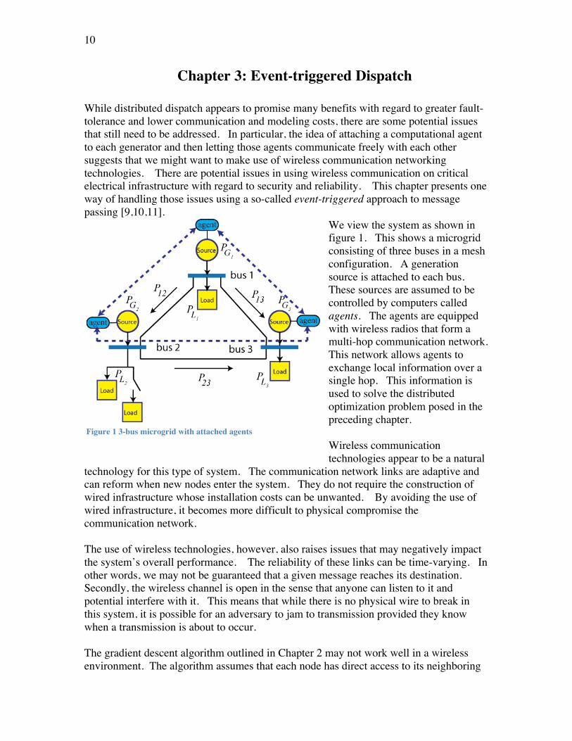
While distributed dispatch appears to promise many benefits with regard to greater fault-tolerance and lower communication and modeling costs, there are some potential issues that still need to be addressed. In particular, the idea of attaching a computational agent to each generator and then letting those agents communicate freely with each other suggests that we might want to make use of wireless communication networking technologies. There are potential issues in using wireless communication on critical electrical infrastructure with regard to security and reliability. This chapter presents one way of handling those issues using a so-called event-triggered approach to message passing [9,10,11].

We view the system as shown in figure 1. This shows a microgrid consisting of three buses in a mesh configuration. A generation source is attached to each bus. These sources are assumed to be controlled by computers called agents. The agents are equipped with wireless radios that form a multi-hop communication network. This network allows agents to exchange local information over a single hop. This information is used to solve the distributed optimization problem posed in the preceding chapter. Wireless communication technologies appear to be a natural

technology for this type of system. The communication network links are adaptive and can reform when new nodes enter the system. They do not require the construction of wired infrastructure whose installation costs can be unwanted. By avoiding the use of wired infrastructure, it becomes more difficult to physical compromise the communication network. The use of wireless technologies, however, also raises issues that may negatively impact the system’s overall performance. The reliability of these links can be time-varying. In other words, we may not be guaranteed that a given message reaches its destination. Secondly, the wireless channel is open in the sense that anyone can listen to it and potential interfere with it. This means that while there is no physical wire to break in this system, it is possible for an adversary to jam to transmission provided they know when a transmission is about to occur. The gradient descent algorithm outlined in Chapter 2 may not work well in a wireless environment. The algorithm assumes that each node has direct access to its neighboring

Figure 1 3-bus microgrid with attached agents

11

node states and line states. This means that each time a generator’s local state is updated; it must first access the state information from its neighbors. In general, these algorithms may require hundreds of updates before converging to the desired solution point, which means frequent requests for neighboring information. The bandwidth requirements for these algorithms, therefore, may quickly overwhelm the capacity of the wireless communication network. One way around this issue is to dramatically reduce the amount of information that has to be exchanged between neighboring agents. This is done by breaking the tight connection between communication and computation in these gradient descent algorithms. Recent work demonstrated that an event-triggering formalism could reduce the required message passing complexity of the algorithm by two orders of magnitude [12,13,14]. Event-triggered message passing has agents broadcast their local states only when some measure of the information novelty in that state exceeds a pre-specified threshold. In other words, these agents broadcast only when they expect their data will have a significant impact on the behavior of their neighbors. By adopting a transmission policy that only sends data when it is needed, we break the tight connection between communication and computation in a manner that greatly reduces the amount of transmitted data. Another interesting feature of event-triggered message passing is that it usually generates sporadic message streams. In other words, the time between consecutive transmissions varies in a random manner that is difficult to predict by an outside observer. This has potential benefits with regard to securing wireless traffic. An easy way of disrupting a wireless network is to set up a narrowband transmitter that jams the transmitter’s broadcast. In cases where transmitters periodically transmit data, it becomes rather easy for an adversary to identify the frequencies and times at which such jamming should be done. Adopting an event-triggered message-passing scheme, however, results in a sporadic scheme in which 1) very few messages are passed and 2) the time between broadcasts is difficult to predict. This means that event-triggered message passing will make it difficult for adversaries to determine the best time to activate their jamming systems. Event-triggered message passing, therefore, may be able to improve the security of such wireless systems to outside interference. The gradient descent algorithm assumes that generator i updates its state using information for its neighbors’ states. As noted above, this would require frequent message passing between agents. An event-triggered version of the update equation assumes that generator i only accesses a sampled version of its neighbor’s state. In particular, let’s associate a sequence of sampling instants,

€

Ti [ ]{ }=0

∞, with the ith

generator. The time

€

Ti [ ] denotes the instant when the ith generator samples its state ϕI for the lth time and transmits that state to neighboring generators k∈ N(i). We can see that at any time t, the sampled generator state is a piecewise constant function of time in which

12

€

ˆ ϕ i t( ) =ϕi Ti [ ]( ) for all

€

= 0,1,...,∞ and any time

€

t ∈ Ti[],Ti[ +1][ ]. In this regard the event-triggered version of the gradient descent update’s algorithm now takes the form,

€

θ i(t) = − µ j τ( )A jij∈L( i)∑ + ˆ ϕ k τ( )Bki

k∈N ( i)∑ +ϕi τ( )Bii

⎛

⎝ ⎜ ⎜

⎞

⎠ ⎟ ⎟ dτ

0

t

∫

for all

€

= 0,1,...,∞ and any time

€

t ∈ Ti[],Ti[ +1][ ]. The sequence

€

Ti [ ]{ }=0

∞ represents

the time instants when generator i transmits its “state” to its neighboring generators. Here we assume there is no transmission delay in each of the broadcasts. A systematic method must be used to select the sampling times

€

Ti [ ]{ }=0

∞. The main

consideration is that these sampling times must be chosen to ensure that the “sampled” version of the gradient descent algorithm converges to the optimal dispatch decision. This selection is based on Lyapunov type arguments in which the Lagrangian, L(θ;w), becomes a candidate Lyapunov function for the sampled system. To ensure the algorithm’s convergence, we need to guarantee that the time rate of change in the Lagrangian is always negative. Let’s first define the local variable zi

€

zi(t) = µ j τ( )A jij∈L(k )∑ + ˆ ϕ k τ( )Bki

k∈N ( i)∑ +ϕi τ( )Bii

to simplify the notation in the derivation. We now compute the derivative of Lagrangian. In particular, for all t > 0, we have

€

− ˙ L θ,w( ) = −∂L∂θ i

dθ i

dti=1

N

∑ = zi µ j A jij∈L(i)∑ + ϕkBki

k∈N (i)∑ +ϕiBii

⎛

⎝ ⎜ ⎜

⎞

⎠ ⎟ ⎟

i=1

N

∑

≥12

zi2 − ϕk − ˆ ϕ k( )Bki

k∈N (i)∑

⎛

⎝ ⎜ ⎜

⎞

⎠ ⎟ ⎟

2⎛

⎝

⎜ ⎜

⎞

⎠

⎟ ⎟

i=1

N

∑ ≥12

zi2

i=1

N

∑ −12

N(k) Bik2

k =1

N

∑⎛

⎝ ⎜

⎞

⎠ ⎟

i=1

N

∑ ϕk − ˆ ϕ k( )2

The preceding equation shows that

€

˙ L θ;w( ) is negative provided

€

zi2 − N(k)Bki

2

k=1

N

∑⎛

⎝ ⎜

⎞

⎠ ⎟ ϕi − ˆ ϕ i( )2

≥ 0

for each generator i. Note that this requirement only requires information available to the ith generator. Moreover, we can recast this inequality as a thresholding condition of the form

€

ϕi(t) − ˆ ϕ i(t) ≤ ρi zi(t) where

€

ρi = N(k)Bik2

k=1

N

∑⎛

⎝ ⎜

⎞

⎠ ⎟

−1

is a constant. The thresholding condition given above requires that generator i transmit its local state when the difference (gap) between the current local state of the generator and the last transmitted state of the generator exceeds the state-dependent threshold

€

ρi zi .

13

This ensures that the transmission time sequences

€

Ti [ ]{ }=0

∞ are chosen so that

€

˙ L θ;w( ) is negative. So the Lagrangian becomes a Lyapunov function for the sampled gradient descent system and we can guarantee that this system converges to the optimal dispatch states. As it turns out the proposed event-triggered dispatch algorithm can be easily integrated into the power inverter controller developed by UWM [2]. This is done by dynamically adjusting the requested power for each generator. In the microsource power inverters, each generator’s phase angle, θi, is adjusted by comparing the measured active power and the requested power so that the phase angle follows the differential equation

€

˙ θ i(t) = π Preq,i − PGi(t)( ) This suggests that if instead of fixing Preq,I , we can adjust it in a dynamic manner so that the θi(t) follows the sampled gradient update algorithm, then the requested power at each generator should converge to a value that globally minimizes the overall system’s operational costs subject to the generator/line power constraints inherent in the network. In particular, this is done by setting

€

Preq,i(t) = PGi(t) −γzi(t)π

where γ>0 is a constant that controls how fast we adjust the phase angle. This constant is needed because if zi(t) is adjusted too fast, then we may destabilize the entire system. Since generator I can compute both PGi and z,I locally, this means that Preq,I can be easily computed by generator i itself. This suggests that each generator only needs to adjust its power set point according to the above equation. It samples and then broadcasts its state ϕI to its neighboring generators when the event-triggering inequality is violated. If every generator follows this action, then our prior analysis guarantees that the generated power of all generators in the system should approach the solution to the optimal power dispatch problem.

14

Chapter 4 Event-triggered Simulations This chapter presents simulation results supporting the correctness of the proposed event-triggered dispatch algorithm. The results in this chapter originally appeared in [4]. The simulation used here was a Matlab simPower simulation of the islanded microgrid shown in figure 2. The scenario chosen here assumes that the event-triggered dispatch algorithm is started at t=3 seconds and then an extra load is added at 10 seconds into the simulation. The cost functions were chosen so that generator 2 is the most expensive generator to operate and the distribution line between bus 3 and bus 2 is flow limited.

Results from this simulation are shown in figure 3. The power generated by each of the generators is shown in the plots as a function of time. As one can see, the optimal dispatcher is switched on at time t=3. Since generator 2 is the most expensive one to operate, we see generator 1 increase its power level and generator 2 reduce its dispatched power. At time t=10 seconds, an extra load is switched onto bus 2. In this case, however, the tie line between bus 3 and 2 is already fully loaded. Generator 1 cannot increase its output because it is already at its limit. Therefore generator 2 increases its power level, even though it is the most expensive generator to operate. These plots suggest that the proposed event-triggered dispatch

algorithm is operating as expected. The next plot to the right shows the communication cost associated with the event-triggered dispatch algorithm. This figure plots the time since last broadcast for each of the generators. The actual broadcast times occur at the discontinuous jumps in the curve. Notice that in all cases, the generators only broadcast when an event occurs. These events correspond to the activation of the optimal dispatcher and the abrupt change in load on bus 2. The important

Figure 2 3-bus microgrid used in event-triggered simulations

Figure 3 simulation result showing time history of generator power

Figure 4: simulation result plotting the time since last broadcast for event-triggered simulation

15

thing to note as that the time between successive broadcasts is usually very long. Indeed only a dozen messages were passed between the 3 generators during this simulation. So the approaches benefits with regard to reducing communication traffic are indeed realized. The remainder of this chapter describes the simPower simulation that was used to obtain the preceding results. This simulation serves as the starting point for the microgrid simulation being developed under this project. So a description of this early simulation model will be useful in highlighting the new features of this project’s simulation.

The top-level simPower model for this microgrid is shown to the left. The upper left hand corner shows the connection to the main grid. Bus 1 is shown on the top, bus 2 on the lower left and bus 3 on the lower right side of the figure. The main block of interest is the generator block.

Expanding out the generator block yields the simPower model shown on the right. Main blocks of interest include the central block, which contains the UWM controller logic,

and the lower block for the event trigger. This event-triggering block realized the decision logic discussed in the preceding chapter. It was implemented as an S-function block. The UWM control logic was realized as a Matlab Simulink model shown to the left. It is

similar to the simulink model developed by UIUC under phase I of this project with some minor modifications that were needed to support the event-triggered dispatching system.

While this simulation worked well in demonstrating the effectiveness of the

event-triggered dispatch algorithm, it was insufficient for the needs of this project. The preceding models lacked sufficient modularity to enable the straightforward

integration of different generation sources.

Figure 5: top-level simPower model for 3-bus mesh microgrid used in event-triggered dispatch

Figure 6: generator simPower model for event-triggered simulation

Figure 7: UWM controller logic (simulink model)

16

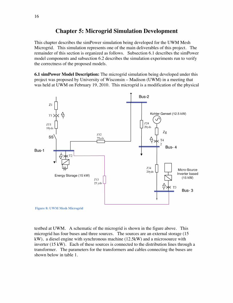
Chapter 5: Microgrid Simulation Development This chapter describes the simPower simulation being developed for the UWM Mesh Microgrid. This simulation represents one of the main deliverables of this project. The remainder of this section is organized as follows. Subsection 6.1 describes the simPower model components and subsection 6.2 describes the simulation experiments run to verify the correctness of the proposed models. 6.1 simPower Model Description: The microgrid simulation being developed under this project was proposed by University of Wisconsin – Madison (UWM) in a meeting that was held at UWM on February 19, 2010. This microgrid is a modification of the physical

testbed at UWM. A schematic of the microgrid is shown in the figure above. This microgrid has four buses and three sources. The sources are an external storage (15 kW), a diesel engine with synchronous machine (12.5kW) and a microsource with inverter (15 kW). Each of these sources is connected to the distribution lines through a transformer. The parameters for the transformers and cables connecting the buses are shown below in table 1.

Figure 8: UWM Mesh Microgrid

17

cables Length yds R - ohms X - ohms Z1 0.0934 0.0255 ZT1 5 0.0028 0.00068 Z12 50 0.0274 0.0066 Z24 30 0.0168 0.0041 Z34 30 0.0168 0.0041 Z13 25 0.0137 0.0033 Zg 0.0656 0.0021 Trans0former voltage KVA Primary

R - pu Primary X - pu

Secondary R - pu

Secondary X - pu

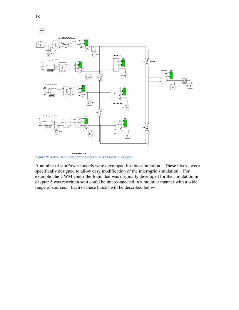
T1 480-208 75 0.0169 0.0676 0.0003 0.0127 T2-T4 480-208 45 0.0269 0.1075 0.0050 0.0201 Table 1: UWM Mesh Microgrid Parameters A simPower model of this microgrid was developed. The diagram for this model is shown below in figure 9. The main grid blocks are shown on the upper left hand side of the figure. The three other generators in this microgrid are on the left hand side of the figure and the loads are shown on the right hand side. This microgrid has two microsources (480 V and 15 kW) and one diesel generator (480 V and 12.5 kW). At the time of the writing of this report, a preliminary model of the external storage source had been developed. This external source model has yet to be integrated into the microgrid simulation. Note that after each coupling transformer, one finds an RC tank circuit that is connected to ground as a load absorbing 100 W and 10 kVAR. This tank circuit was used to reduce switching transients that occur when the system islands. The loads on bus 1 and bus 3 are 5 kW each. The load on bus 2 is 10 kW. Bus 4 has 10 kW load that increases to 13 kW at 2 seconds into the simulation.

18

Figure 9: Notre Dame simPower model of UWM mesh microgrid

A number of simPower models were developed for this simulation. These blocks were specifically designed to allow easy modification of the microgrid simulation. For example, the UWM controller logic that was originally developed for the simulation in chapter 5 was rewritten so it could be interconnected in a modular manner with a wide range of sources. Each of these blocks will be described below.

19

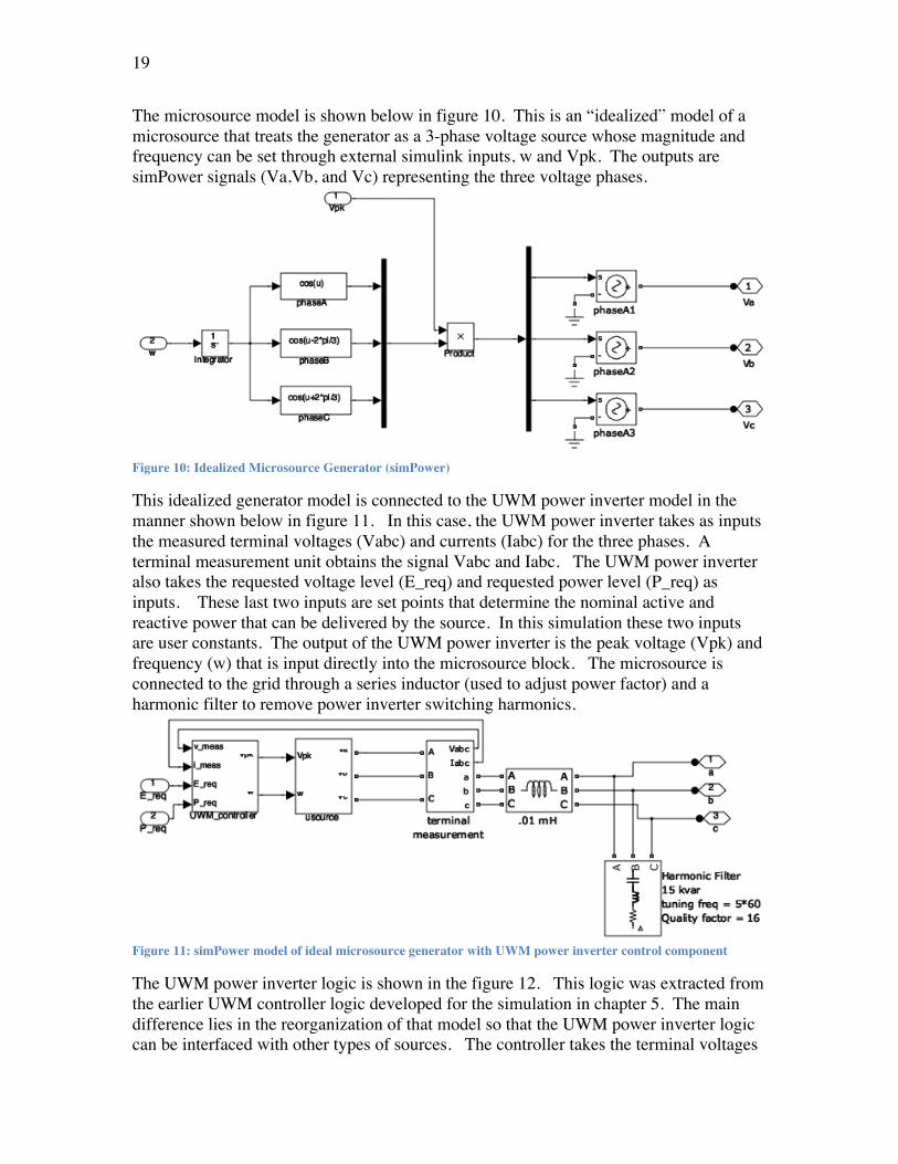
The microsource model is shown below in figure 10. This is an “idealized” model of a microsource that treats the generator as a 3-phase voltage source whose magnitude and frequency can be set through external simulink inputs, w and Vpk. The outputs are simPower signals (Va,Vb, and Vc) representing the three voltage phases.

Figure 10: Idealized Microsource Generator (simPower)

This idealized generator model is connected to the UWM power inverter model in the manner shown below in figure 11. In this case, the UWM power inverter takes as inputs the measured terminal voltages (Vabc) and currents (Iabc) for the three phases. A terminal measurement unit obtains the signal Vabc and Iabc. The UWM power inverter also takes the requested voltage level (E_req) and requested power level (P_req) as inputs. These last two inputs are set points that determine the nominal active and reactive power that can be delivered by the source. In this simulation these two inputs are user constants. The output of the UWM power inverter is the peak voltage (Vpk) and frequency (w) that is input directly into the microsource block. The microsource is connected to the grid through a series inductor (used to adjust power factor) and a harmonic filter to remove power inverter switching harmonics.

Figure 11: simPower model of ideal microsource generator with UWM power inverter control component

The UWM power inverter logic is shown in the figure 12. This logic was extracted from the earlier UWM controller logic developed for the simulation in chapter 5. The main difference lies in the reorganization of that model so that the UWM power inverter logic can be interfaced with other types of sources. The controller takes the terminal voltages

20

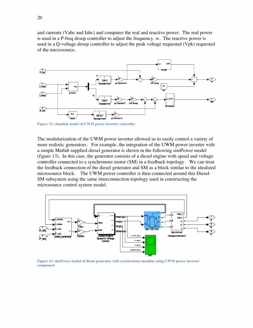
and currents (Vabc and Iabc) and computes the real and reactive power. The real power is used in a P-freq droop controller to adjust the frequency, w. The reactive power is used in a Q-voltage droop controller to adjust the peak voltage requested (Vpk) requested of the microsource.

Figure 12: simulink model of UWM power inverter controller

The modularization of the UWM power inverter allowed us to easily control a variety of more realistic generators. For example, the integration of the UWM power inverter with a simple Matlab supplied diesel generator is shown in the following simPower model (figure 13). In this case, the generator consists of a diesel engine with speed and voltage controller connected to a synchronous motor (SM) in a feedback topology. We can treat the feedback connection of the diesel generator and SM as a block similar to the idealized microsource block. The UWM power controller is then connected around this Diesel-SM subsystem using the same interconnection topology used in constructing the microsource control system model.

Figure 13: simPower model of diesel generator with synchronous machine using UWM power inverter component

21

A similar approach can be taken to integrate the UWM power inverter with a three phase external source. This interconnection is shown in figure 14. The novel component in the 3-phase storage source is the

UWM power inverter logic and the source model. In particular, the

battery model needs to capture the charge/discharge behavior of the battery as well as some modifications to the UWM controller logic. At the time of writing this report, a preliminary version of the battery model was completed, but the UWM controller modifications had not yet been completed. The simPower models for the 3-phase storage component and its associated battery model are shown in figure 15.

6.2: simPower Simulation Experimental Results Initial simulation runs with the simPower model in figure 8 appear to be consistent with similar simulation runs presented by UWM in February of 2010. The simulation described in this section assumes that the system is initially connected to the main grid, with additional sources generating with two microsources with peak power of 15 kW a piece (on bus 1 and bus 3) and a diesel generator (SM) with 12.5 kW peak power (bus 4). The main grid is connected to bus 1 and the microgrid islands from the main grid at 1 second. Loads are connected to all four buses. Bus 1 has 5 kW, bus 2 has 10 kW, bus 4 has 5 kW and bus 2 starts out at 10 kW but increases to 13 kW at 2 seconds into the simulation. Figure 16 shows the current drawn from the main grid. There is an initial startup transient between 0 to .75 seconds. When the microgrid islands at 1 second, the current leaving the main grid drops to zero, as would be expected.

Figure 16: main grid current time history

Figure 14: simPower model of external storage device controlled by UWM power inverter

Figure 15: simPower model of battery

22

Figure 17 shows the current drawn by bus 2’s load as well as the real power delivered to this load. After an initial startup transient, the power drawn by this load settles at around 10 kW with a peak-peak current of about 50 amps. At 2 seconds, this peak power level jumps to 13-14 kW with a similar increase in current. These results suggest that the simulation is operating as expected.

Figure 17: bus 2 current and power

The generated power from each source in the microgrid is shown in the figure 18 (left). This plot shows that under islanding, there is little change in the generated power levels. This is because the requested power levels for all generators was set to one p.u.. After the load changes on bus 2 at t=2, then there is a small increase in generated power that is equally distributed between the three sources.

Figure 18: distributed generator power delivered

23

The final set of plots in figure 19 show the response of the loads. The left hand plots are for the voltages (Vabc) of the three phases. Note that through the islanding and load change these voltage levels change very little, thereby indicating that the control system was able to maintain voltage power quality. The right hand plots show the frequency on the load buses. The only under frequency condition occurs when the system was initially started. After the startup transient, however, the frequency shows no appreciable variation through islanding and bus 2 load change.

Figure 19: load bus voltages and frequency

The simulation results in this chapter represent initial tests of the simPower microgrid model. These simulations were primarily done to verify the functionality of the UWM power inverter components. These preliminary simulation studies suggest that the simPower model is functioning correctly. Additional simulation studies are planned to provide a more comprehensive test of the simPower models.

24

Chapter 6: Conclusions This report documents the work performed by the University of Notre Dame from July 1st 2010 to September 1st 2010. During this period the following things were achieved

• simPower model of the UWM power inverter controller was constructed • simPower models of a power inverter controlled idealized microsource, diesel

generator and synchronous machine, and external storage battery were constructed

• simPower model of a mesh microgrid proposed by UWM in February 2010 was constructed and tested. This microgrid model used two microsources and one diesel generator synchronous machine. The external storage source was not used in this model because the model still needed additional testing. Preliminary results with this microgrid model are consistent with data provided earlier by UWM.

• An event-triggered distributed algorithm for optimal power dispatch was designed and tested in a simPower simulation of a mesh microgrid. The results of this work were presented in the American Control Conference, June 2010, in Baltimore Maryland [4].

Most of Notre Dame’s objectives were met over this period. Simulation objectives that remain to be completed are

• Integration of the external storage source into the mesh microgrid • Development of simPower models for event-triggered dispatch algorithm • Design of intelligent load shedding algorithms • Simulation testing of load shedding algorithms • Providing support to Odyssian regarding embedded control algorithm

implementation and wireless networking implementation. These remaining objectives are consistent with the revised project milestones provided by

Odyssian Technologies.

25

References

[1] R. Lasseter and P. Paigi, “Microgrid: a conceptual solution”, in Power Electronics Specialists Conference, 2004, PESC 04, 2004 IEEE 35th Annual, volume 6, June 2004, pages 4285-4290 [2] R. Lasseter, “Control and Design of Microgrid Components”, Final Project Report, PSERC publication 06-03, January 2006 [3] F. Katiraei, M.R. Iravani, and P.W. Lehn, “Micro-grid autonomous operation during and subsequent to islanding process”, IEEE Transactions on Power Delivery, volume 20, number 1, pp 248-257, 2005 [4] P. Wan and M.D. Lemmon (2010), Optimal power flow in microgrids using event-triggered optimization , American Control Conference, Baltimore, USA, 2010 [5] F. Kelly, A. Maulloo, and D. Tan, “Rate control for communication networks: shadow prices, proportional fairness and stability,” Journal of the Operational Research Society, vol. 49, no. 3, pp. 237–252, 1998. [6] S. Low and D. Lapsley, “Optimization flow control, I: basic algorithm and convergence,” IEEE/ACM Transactions on Networking (TON), vol. 7, no. 6, pp. 861–874, 1999. [7] J. Wen and M. Arcak, “A unifying passivity framework for network flow control,” Automatic Control, IEEE Transactions on, vol. 49, no. 2, pp. 162–174, 2004. [8] D. Palomar and M. Chiang, “Alternative Distributed Algorithms for Network Utility Maximization: Framework and Applications,” Auto- matic Control, IEEE Transactions on, vol. 52, no. 12, pp. 2254–2269, 2007. [9] Tabuada, “Event-triggered real-time scheduling of stabilizing control tasks,” IEEE transactions on automatic control, vol. 52, no. 9, p. 1680, 2007. [10] X. Wang and M. Lemmon, “Self-triggered feedback control systems with finite-gain l 2 stability,” IEEE transactions on automatic control, vol. 54, p. 452, 2009. [11] X. Wang and M. Lemmon, “Event-triggering in distributed networked systems with data dropouts and delays,” in Proceedings of Hybrid Systems: computation and control, 2009. [12] P. Wan and M.D. Lemmon (2009), An event-triggered distributed primal-dual algorithm for network utility maximization, IEEE Conference on Decision and Control (CDC), Shanghai, PRC, December 2009. [13] P. Wan and M. Lemmon (2009), Event triggered distributed optimization in sensor networks , Information Processing in Sensor Networks (IPSN), 2009. [14] P. Wan and M. Lemmon (2009), Distributed Network Utility Maximization using Event-triggered augmented Lagrangian methods, American Control Conference, 2009.