ADVANCED DIAGNOSTIC TECHNIQUES FOR THREE-PHASE …/67531/metadc782459/m2/1/high... · ADVANCED...
88
ADVANCED DIAGNOSTIC TECHNIQUES FOR THREE-PHASE SLURRY BUBBLE COLUMN REACTORS (SBCR) Annual Technical Progress Report No. 3 for the Period July 1, 2001 – June 30, 2002 DE-FG-26-99FT40594 Principal Investigator: M.H. Al-Dahhan Washington University Associate Professor and Associate Director Department of Chemical Engineering Chemical Reaction Engineering Laboratory Campus Box 1198 One Brookings Drive St. Louis, Missouri 63130 Fax: 314-935-4832 Phone: 314-935-7187 E-mail: [email protected] Co-Investigators: L.-S. Fan Ohio State University Distinguished University Professor Department of Chemical Engineering Chairman, Department of Chemical 140 West 19 th Avenue-Room 125 Engineering Columbus, Ohio 43210-1180 Fax: 614-292-3769 Phone: 614-292-7907 E-mail: [email protected] M.P. Dudukovic Washington University The Laura and William Jens Department of Chemical Engineering Professor and Chairman Campus Box 1198 Director, Chemical Reaction Engineering One Brookings Drive Laboratory St. Louis, Missouri 63130 Fax: 314-935-4832 Phone: 314-935-6021 E-mail: [email protected] Industrial Collaborator B. Toseland Air Products and Chemicals Students Washington University: Ashfaq Shaikh, N. Rados, David Newton Ohio State University: R.Lau, K.Vuong, Q. Marshdeh, R.Ahmed July 25, 2002 Prepared for the United States Department of Energy Award No. DE-FG-26-99FT40594 Award Period: July 1, 2001 – June 30, 2002
Transcript of ADVANCED DIAGNOSTIC TECHNIQUES FOR THREE-PHASE …/67531/metadc782459/m2/1/high... · ADVANCED...

ADVANCED DIAGNOSTIC TECHNIQUES FOR THREE-PHASE SLURRY BUBBLE COLUMN REACTORS (SBCR)
Annual Technical Progress Report No. 3
for the Period July 1, 2001 – June 30, 2002 DE-FG-26-99FT40594
Principal Investigator:
M.H. Al-Dahhan Washington University Associate Professor and Associate Director Department of Chemical Engineering Chemical Reaction Engineering Laboratory Campus Box 1198 One Brookings Drive St. Louis, Missouri 63130 Fax: 314-935-4832 Phone: 314-935-7187 E-mail: [email protected]
Co-Investigators:
L.-S. Fan Ohio State University Distinguished University Professor Department of Chemical Engineering Chairman, Department of Chemical 140 West 19th Avenue-Room 125 Engineering Columbus, Ohio 43210-1180 Fax: 614-292-3769 Phone: 614-292-7907 E-mail: [email protected]
M.P. Dudukovic Washington University The Laura and William Jens Department of Chemical Engineering Professor and Chairman Campus Box 1198 Director, Chemical Reaction Engineering One Brookings Drive Laboratory St. Louis, Missouri 63130 Fax: 314-935-4832 Phone: 314-935-6021 E-mail: [email protected] Industrial Collaborator
B. Toseland Air Products and Chemicals
Students
Washington University: Ashfaq Shaikh, N. Rados, David Newton Ohio State University: R.Lau, K.Vuong, Q. Marshdeh, R.Ahmed
July 25, 2002
Prepared for the United States Department of Energy Award No. DE-FG-26-99FT40594
Award Period: July 1, 2001 – June 30, 2002

Disclaimer This report was prepared as an account of work sponsored by an agency of the United States Government. Neither the United States Government nor any agency therefore, nor any of their employees, makes any warranty, express or implied, or assumes any legal liability or responsibility for the accuracy, completeness, or usefulness of any information, apparatus, product, or process disclosed, or represents that its use would not infringe privately owned rights. Reference herein to any specific commercial product, process, or service by trade name, trademark, manufacturer, or otherwise does not necessarily constitute or imply its endorsement, recommendation or favoring by the United States Government or any agency thereof. The views and opinions of authors expressed herein do not necessarily state or reflect those of the United States Government or any agency thereof.
ii

ADVANCED DIAGNOSTIC TECHNIQUES FOR THREE-PHASE SLURRY BUBBLE COLUMN REACTORS (SBCR)
Annual Technical Progress Report No. 3
for the Period July 1, 2001 – June 30, 2002 DE-FG-26-99FT40594
ABSTRACT
This report summarizes the accomplishment made during the third year of this cooperative research effort between Washington University, Ohio State University and Air Products and Chemicals. Data processing of the performed Computer Automated Radioactive Particle Tracking (CARPT) experiments in 6” column using air-water-glass beads (150µm) system has been completed. Experimental investigation of time averaged three phases distribution in air-Therminol LT-glass beads (150µm) system in 6” column has been executed. Data processing and analysis of all the performed Computed Tomography (CT) experiments have been completed, using the newly proposed CT/Overall gas holdup methodology. The hydrodynamics of air-Norpar 15-glass beads (150µm) have been investigated in 2” slurry bubble column using Dynamic Gas Disengagement (DGD), Pressure Drop fluctuations, and Fiber Optic Probe. To improve the design and scale-up of bubble column reactors, a correlation for overall gas holdup has been proposed based on Artificial Neural Network and Dimensional Analysis.
iii

ADVANCED DIAGNOSTIC TECHNIQUES FOR THREE-PHASE SLURRY BUBBLE COLUMN REACTORS (SBCR)
Annual Technical Progress Report No. 3
for the Period July 1, 2001 – June 30, 2002 DE-FG-26-99FT40594
TABLE OF CONTENTS
Page No. Disclaimer ii Abstract iii Table of Contents iv List of Figures vi Executive Summary viii 1.
INTRODUCTION AND MOTIVATION
1
2.
OVERALL OBJECTIVES
3
2.1 Accomplishments During the First Year 3 2.2 Accomplishments During the Second Year 4 2.3 Accomplishments During the Third Year 4 2.4 Plan for Next Year at no-cost extension 5 3.
EXPERIMENTAL FACILITY
6
3.1 High pressure and high temperature 2” diameter slurry bubble column
6
3.2 High pressure 6” diameter slurry bubble column 6 3.3 Dynamic Gas Disengagement (DGD) 7 3.4 Fiber Optic Probe 7 3.5 Computer Automated Radioactive Particle Tracking
(CARPT) 8
3.6 Computed Tomography (CT) 9 4.
RESULTS AND DISCUSSIONS
22
4.1 Hydrodynamics measurements in 2” column using DGD, ∆P Fluctuation, and Fiber Optic Probe
22
4.1.1 Overall gas holdup using DGD 4.1.2 Prediction of regime transition using ∆P fluctuations 4.1.3 Bubble Size and Bubble Rise Velocity 4.2 Hydrodynamics Measurements in 6” column using CARPT
and CT
27 4.2.1 Results of CT (gas holdup profile)/CARPT (solids
axial velocity profile and turbulent parameters)Using Air-Water-Glass Beads System
iv

4.2.2 Results of CT (gas and solids holdup profile) Using
Air-Therminol LT-Glass Beads System
5.
DEVELOPMENT OF ARTIFICIAL NEURAL NETWORK CORRELATION FOR PREDICTION OF OVERALL GAS HOLDUP IN BUBBLE COLUMNS
36 6.
NOMENCLATURE AND REFERENCES
37
6.1 NOMENCLATURE 37 6.2 REFERENCES 38 7.
APPENDIX A
40
v

LIST OF FIGURES Figure No. Caption Page No. Figure 1.1 Effect of Design Parameters, Operating Variables, Phase
Physical Properties and Kinetics on the Slurry Bubble Column Yield and Selectivity
2
Figure 3.1 Schematic diagram for high pressure and high temperature slurry bubble column
16
Figure 3.2 Gas flowsheet for the high pressure 6 inch diameter bubble column
17
Figure 3.3 Bubble column reactor of 6” without ports used for CARPT/CT measurements. CT1, CT2, and CT3 represents the scan levels used in this investigation
18 Figure 3.4 Bubble column reactor of 6” with ports used for overall gas
holdup and DP measurements. CT1, CT2, and CT3 represents the scan levels used in this investigation.
19 Figure 3.5 Typical variation of dynamic pressure gradient with time
during the bed disengagement process.
20 Figure 3.6 Schematic diagram of the U-shaped optical fiber probe 20 Figure 3.7 Configuration of the CARPT experimental setup 21 Figure 3.8 Configuration of the CT experimental setup (Kumar, 1994) 21 Figure 4.1 Effect of pressure on overall gas holdup (Nitrogen - Norpar 15
- 150µm glass beads) at various solids loading
23 Figure 4.2 Effect of solids loading on gas holdup (Nitrogen – Norpar 15 –
150µm glass beads) at various operating pressures
24 Figure 4.3 Effect of a) solids loading and b) operating pressure on regime
transition using Nitrogen – Norpar 15 – 150µm glass beads in 2” column
25 Figure 4.4 Effect of solids loading on bubble size using Nitrogen - Norpar
15 - 150 µm glass beads in 2” column at Ug = 30 cm/s, P = 1.78 MPa
26 Figure 4.5 Effect of solids loading on bubble rise velocity using Nitrogen
- Norpar 15 - 150 µm glass beads in 2” column at Ug = 30 cm/s, P = 1.78 MPa
27 Figure 4.6 Effect of superficial gas velocity on gas holdup profile (air-
water-glass beads 150 µm) in 6” column with 9.1 % vol. solids loading at 0.1 MPa
28 Figure 4.7 Effect of superficial gas velocity on solids axial velocity
profile (air-water-glass beads 150 µm) in 6” column with 9.1 % vol. solids loading at 0.1 MPa
28 Figure 4.8 Effect of superficial gas velocity on solids shear stress profile
(air-water-glass beads 150 µm) in 6” column with 9.1 % vol. solids loading at 0.1 MPa
29 Figure 4.9 Effect of superficial gas velocity on TKE (air-water-glass
beads 150 µm) in 6” column with 9.1 % vol. solids loading at 0.1 MPa
29
vi

Figure 4.10 Effect of superficial gas velocity on a) solids axial diffusivity, and b) solids radial diffusivity (air-water-glass beads 150 µm) in 6” column with 9.1 % vol. Solids loading at 0.1 MPa
30 Figure 4.11 Effect of operating pressure on gas holdup radial profile using
air-water-glass beads (150 µm) in 6” column with 9.1 % vol. solids loading at 45 cm/s
31 Figure 4.12 Effect of operating pressure on axial velocity profile using air-
water-glass beads (150 µm) in 6” column with 9.1 % vol. solids loading at 45 cm/s
31 Figure 4.13 Effect of operating pressure on solids shear stress profile using
air-water-glass beads (150 µm) in 6” column with 9.1 % vol. solids loading at 45 cm/s
32 Figure 4.14 Effect of operating pressure on solids TKE using air-water-
glass beads (150 µm) in 6” column with 9.1 % vol. solids loading at 8 and 45 cm/s
32 Figure 4.15 Effect of operating pressure on a) solids axial diffusivity
profile b) solids radial diffusivity profile using air-water-glass beads (150 µm) in 6” column with 9.1 % vol. solids loading at 8 and 45 cm/s
33 Figure 4.16 Effect of superficial gas velocity on a) gas holdup, and b)
solids holdup profile (air – Therminol LT-glass beads) in 6” column with 9.1 % vol. solids loading at 0.1 MPa.
34 Figure 4.17 Effect of operating pressure on a) gas holdup, and b) solids
holdup profile (air– Therminol LT-glass beads) in 6” column with 9.1 % vol. solids loading at 14 cm/s.
35
vii

ADVANCED DIAGNOSTIC TECHNIQUES FOR THREE-PHASE SLURRY BUBBLE COLUMN REACTORS (SBCR)
Annual Technical Progress Report No. 3
for the Period July 1, 2001 – June 30, 2002 DE-FG-26-99FT40594
EXECUTIVE SUMMARY
The overall objective of this cooperative research effort between Washington University, Ohio State University and Air Products and Chemicals is to advance the understanding of the hydrodynamics of Fischer-Tropsch (FT) Slurry Bubble Column Reactors (SBCR) via advanced diagnostic techniques. The emphasis during this third year was: i) to complete data processing and analysis of the performed Computer Automated Radioactive Particle Tracking (CARPT) experiments in 6” column using air-water-glass beads (150 µm), ii) to complete data processing and analysis of the performed Computed Tomography (CT) experiments of air-water-glass beads (150 µm) in 6” column using the newly proposed CT/Overall gas holdup methodology, iii) to investigate the time averaged three phases distribution of air-Therminol LT-glass beads (150 µm) system in 6” column using CT and to process the obtained data using CT/Overall gas holdup methodology, iv) to investigate the hydrodynamics of air-Norpar 15-glass beads (150 µm) system in 2” column using Dynamic Gas Disengagement (DGD), Pressure drop fluctuations, and Fiber Optic Probe, v) to develop a correlation to predict overall gas holdup in bubble columns based on Artificial Neural Network and Dimensional Analysis. This report summarizes the accomplishments made during the third year of this project. The report is organized in individual sections. The following is an outline of each section. Section 1 provides an introduction and motivation for this collaborative project. Section 2 provides a review of the objectives and tasks set for the project, list of accomplishments during the first, second, and third year and plan for the next no-cost extension year. Section 3 describes the experimental facilities at Washington University and Ohio State University and the advanced techniques (Fiber Optic Probe, Pressure Drop fluctuation, DGD, CARPT, CT) used to study the hydrodynamics of high pressure slurry bubble column. Section 4 discusses the results and the findings of the performed experiments at Ohio State University and Washington University. Section 5 - Appendix A provides details for the development of the overall gas holdup correlation in bubble columns for a wide range of conditions based on Artificial Neural network.
viii

1. INTRODUCTION AND MOTIVATION Synthesis gas (mixture of carbon monoxide and hydrogen) from coal and natural gas is one of the most abundant and reliable sources of energy and chemicals. Fischer-Tropsch (FT) Chemistry is an acknowledged route for clean utilization of coal/natural gas-derived synthesis gas in production of fuels and chemicals. Based on reaction engineering considerations and economic point of view, slurry bubble column reactors (SBCR) operated at high gas velocities in churn turbulent flow regime are the preferred reactors for commercialization of FT synthesis. Slurry bubble column is a cylindrical vessel in which gas is sparged using a distributor (sparger) into a suspension (slurry) of liquid and solid particles. The slurry phase flow can be either co-current, counter-current or in batch mode with respect to the gas flow. The size of the solid particles ranges from 5 to 150 µm and solids loading up to 50 % volume (Krishna et al., 1997). Gas phase contains one or more reactants (e.g. synthesis gas for FT processes) while liquid phase usually contains product, and/or reactants (or sometimes inert). The solid particles are typically catalyst (or product). The main advantages of slurry reactors (compared to agitated reactors) are excellent mixing without moving parts (smaller capital and maintenance costs) and much lower power consumption. Such an excellent mixing characteristics lead to good heat, and mass transfer and hence, improved production. One of the main disadvantages of slurry bubble column reactors is significant back-mixing which can affect product conversion. In SBCR, momentum is transferred from the faster, upward moving, gas phase to the slower liquid and solid phases. As long as the operating liquid superficial velocity (in the range of 0 to 2 cm/s) has an order of magnitude smaller than the superficial velocity of the gas (1 to 30 cm/s), and the catalyst particles are small (less than 50 µm), the gas dominates the hydrodynamics. There are considerable reactor design and scale-up problems associated with FT synthesis technology. The large gas throughputs necessitate the use of large diameter reactors (typically 5 – 8 m). The process operates under high-pressure conditions (typically 10 – 80 bar). In order to achieve economically high space-time yields, high slurry concentration (typically 30 – 50 % vol.) needs to be employed. To obtain high conversion levels, large reactor heights, typically 20 – 30 m tall are required. Finally, FT processes are exothermic in nature, and hence they need efficient means of heat removal. Successful commercialization of the slurry bubble column reactor (SBCR) technology for FT is crucially dependent on the proper understanding of the scale-up principles. Despite the simple mechanical design of SBCR, the flow field and fluid dynamics are still not well understood due to the complex interaction among the three phases. As it can be seen from Figure 1.1 many design, operating, physical property and kinetic variables affect the SBCR performance (yield and selectivity). Hence, reliable design and scale-up methodology need improved understanding and quantification of the key hydrodynamic phenomena (Deckwer, 1993). However, reliable data and tested models or theories for quantification of hydrodynamics of slurry bubble column reactor are still scarce and therefore a reliable and validated methodology for scale-up of FT SBCR is not yet available.
1

Operating Variables• gas flow rate• liquid flow rate• catalyst renewal rate• feed temperature• feed composition• system temperature• system pressure
Phase Physical Properties
Slurry Bubble Column Operation• bubble (growth, interaction, dispersion)• gas holdup profiles• solids (catalyst) holdup profiles• velocity profiles• flow regime• mixing properties• heat transfer• mass transfer
Yield and SelectivityYield and Selectivity
KineticsKinetics
Design Parameters• reactor geometry• reactor internals• sparger design• catalyst size• catalyst loading• heating/cooling duty
Design Parameters• reactor geometry• reactor internals• sparger design• catalyst size• catalyst loading• heating/cooling duty
Figure 1.1: Effect of Design Parameters, Operating Variables, Phase Physical Properties and Kinetics on the Slurry Bubble Column Yield and Selectivity
Therefore, the overall objective of this project is to quantify the SBCR hydrodynamics by utilizing advanced diagnostic techniques. This can be achieved by properly describing the distribution of phases and liquid (slurry) circulation and turbulence in SBCR for Fischer-Tropsch synthesis via studying the microstructure of the gas-liquid-solid mixtures in a comparable fluid to FT waxes in 2 inch diameter column, developing a fundamental understanding as to how important the physical and fluid dynamic properties can be “finger-printed” via various diagnostic techniques such as laser doppler anemometry (LDA), optical probe and differential pressure fluctuation technique and by measuring large scale hydrodynamic parameters at high pressure and high gas velocity in a 6 inch diameter slurry bubble column using computed tomography (CT) and computer automated radioactive particle tracking (CARPT). CARPT and CT are the only non-invasive techniques that can provide information on slurry velocity and density profiles in 3D domain. Such data provides a firm scientific and engineering basis for scale-up and design of FT SBCR. In addition, the obtained results can be utilized as a benchmark to validate the computational fluid dynamic codes. This grant enables a unique integration of the expertise of the two universities (Washington University, WU and Ohio State University, OSU) and industry (Air Products and Chemicals, APCI) towards achieving the goals set for the project. This study complements well the work performed by WU, OSU, Iowa State University (ISU) and Sandia National Laboratory, Contract No. DE-FC-22-95PC95051, related to the La Porte Advanced Fuels Demonstration Unit (AFDU) operated by Air Products with the Department of Energy funding which focuses on advancing the state-of-the-art in understanding the fluid dynamics of slurry bubble columns and replacing empirical design methods with a more rational approach.
2

2. OBJECTIVES The overall objective of this cooperative university (WU and OSU)-industry (APCI) research is to advance the understanding of the hydrodynamics of FT SBCR via advanced diagnostic techniques. The goals set for this project are as follows: TASK 1: Literature Review
- Physicochemical properties and their effect on the hydrodynamics of bubble columns.
- Models used to predict FT reactor performance.
TASK 2: Based on Task 1, identify the range of intrinsic properties (density, viscosity and surface tension) of the fluids used for the FT synthesis.
- Identify a solvent that, at room temperature and pressure up to 200 psig, will mimic the hydrodynamics of FT wax (at FT reaction conditions).
- Identify the particle type and size to be used.
TASK 3: Using the identified system (solvent-particle-air), perform the following investigations on the hydrodynamics in a 2” diameter column:
- Investigate the effect of reactor pressure on the flow field and turbulent parameters using Laser Doppler Anemometer (LDA).
- Identify the flow regime transition and investigate the effect of reactor pressure on the flow regime transition using ∆P fluctuation measurements.
- Measure overall gas holdup using change in slurry height. - Measure bubble size and bubble rise velocity using Optical Probe.
TASK 4: Using the identified system in Task 2 or a system with similar properties, investigate the hydrodynamics in a 6” diameter column via CT and CARPT techniques. The following will be measured:
- Phase distribution profiles using CT - Flow field and turbulent parameters using CARPT - Gas holdup using CT and change in slurry height.
TASK 5: Evaluate scale-up procedure for slurry bubble column. Develop additional
correlations, if needed.
TASK 6: Final report 2.1 Accomplishments During the First Year
The first year was dedicated for the preparation of the technical review, experimental facilities and the advanced measurement techniques. A new correlation was developed to
3

predict the liquid-solid mass transfer coefficient in high pressure bubble column based on the atmospheric pressure data. The accomplishments were as follows:
The technical review of the variables affecting SBCR performance, some aspects of bubble dynamics and hydrodynamic properties and the physical properties of FT waxes and catalyst has been performed. The experimental facilities and the advanced measurement techniques have been
prepared. The preparation includes the following units: High pressure (up to 3000 psi) and high temperature (up to 250°C) 2-inch diameter
slurry bubble column set-up. High pressure (up to 200 psi) 6-inch diameter slurry bubble column set-up. Two facilities will be used; one for computer automated radioactive particle tracking
(CARPT) and computed tomography (CT) techniques and another one for pressure drop measurements. The later facility consists of a 6-inch diameter column equipped with 6- windows and 15 ports along the column.
Laser Doppler Anemometry (LDA) for 2” slurry bubble column facility. CARPT and CT for 6-inch slurry bubble column facility. Techniques to measure in situ the intrinsic density, viscosity and surface tension of
the selected liquid-phase which mimic the hydrodynamics of FT waxes.
The solvents that mimic FT waxes at FT operating conditions have been identified and the gas and solid phases to be used in the hydrodynamics investigation have been selected. A new correlation to estimate the mass transfer coefficient at high pressure operation
based on atmospheric pressure data has been developed. 2.2 Accomplishments During the Second Year Experimental investigation of the hydrodynamics of Norpar 15- nitrogen-glass beads
in 2” column using LDA/pressure drop/slurry height measurements has been executed. The technical difficulties related to CARPT at high pressure stainless steel SBCR
have been resolved. Experimental investigation of the effect of reactor pressure and gas flow rate on the
hydrodynamics of air-water-glass beads system in 6” column using CT/CARPT has been performed. Correlations to predict radial gas holdup and axial liquid recirculation velocity
profiles in bubble columns have been developed. 2.3 Accomplishments During the Third Year Completion of data processing and analysis of CARPT experiments in 6” column
using air-water-glass beads (150 µm) system has been achieved. Comparison between the proposed CARPT/CT/differential pressure measurements
(DP) and CT/Overall Gas holdup methodologies to compute three phases distribution in air-water-glass beads (150 µm) system in 6” column has been performed. Data
4

processing and analysis have been completed using the developed CT/Overall Gas holdup methodology. Experimental investigation of time averaged three phases distribution of air-
Therminol LT-glass beads (150µm) system in 6” column has been executed using CT. The data processing and analysis of CT experiments have been performed using the developed CT/Overall Gas holdup methodology. Experimental investigation of the hydrodynamics of air-Norpar 15-glass beads (150
µm) in 2” column using Dynamic Gas Disengagement, Pressure Drop fluctuations, and Fiber Optic Probe measurements has been performed. Artificial Neural Network based correlation for prediction of overall gas holdup in
bubble column reactors has been developed. 2.3 Plan for the Next Year of no-cost extension Complete experimental investigation of air-Therminol LT-glass beads (150µm)
system in 6” column using CARPT. Complete data processing and analysis of the performed CARPT experiments. Write final report.
5

3. EXPERIMENTAL FACILITY
The experimental facilities and the diagnostic techniques that are used in the investigation reported in this report are outlined below. 3.1 High pressure and high temperature 2” diameter slurry bubble column [OSU] The schematic diagram of the high pressure and high temperature slurry bubble column is shown in Figure 3.1. The height of the column is 95.9 cm and has an inside diameter of 5.1 cm. There are three pairs of quartz windows installed on the front and rear sides of the column. These windows allow viewing throughout the entire test section of the column. Each window is of 1.27 cm in width and 9.3 cm in height. The maximum operating pressure and temperature of the system are 21 MPa and 180ºC, respectively. Additionally, a perforated plate is used as the gas distributor comprised with 19 triangular pitched holes of 0.45 mm diameter each and 0.156 % open area. A dynamic pressure transducer is installed at 1.0 cm and 20.5 cm above the distributor plate. 3.2 High pressure 6” diameter slurry bubble column [WU] The experimental setup shown in Figure 3.2 was designed to support the maximum operating pressure of 200 psig. The air is supplied from two compressors connected in parallel with the working pressure of 195 psig (1.45 MPa) and the maximum corresponding rated flow rate of 310 SCFM. The compressed atmospheric air is purified, by passing through the dryer and several air filter units. The maximum operational flow rate through the column is about 230 SCFM at atmospheric pressure and about 130 SCFM at 1.0 MPa. The air flow rate is regulated using a pressure regulator and rotameter setup consisting of 4 rotameters of increasing range connected in parallel. Air exits the column through a demister, passes through the back pressure regulator (that controls column operating pressure) and vents to atmosphere. A 16.15 cm (6”) diameter stainless steel bubble column is used in all experiments. Column design enables easy removal of the distributor chamber and sparger replacement. Two similar column designs are used to suit all the needed experiments. The first one, designed for CARPT/CT experiments, is a 6” column equipped with just two probe ports (1”) at each end of the column (i.e. z = 215 cm and z = 12 cm) as shown in Figure 3.3. The second column is used for overall gas holdup and differential pressure (DP) measurements, which has the same dimensions as the first one (Figure 3.4). This column is equipped with an array of additional 15 probe ports (1”) and 6 (12”H x 1½”W) view windows. The three view windows mounted at radially opposite sides are staggered to cover the middle and the top part of the column. View windows are made of tempered quartz glass and are rated to the same pressure as the column itself (200 psig). These windows and 1” ports are mounted on two mutually perpendicular r-z planes. The batch of slurry constitutes the selected solvent as the liquid phase and the selected solid phase.
6

3.3 Dynamic Gas Disengagement (DGD)[OSU] Gas holdup measurement was made using dynamic gas disengagement (DGD) technique. The procedure in the DGD technique includes: 1) the gas supply to the column is suddenly shut off; 2) the gas holdup is continuously measured. A typical DGD curve (pressure drop, (dp/dz) vs. time) for the high pressure slurry bubble column is shown in Figure 3.5. The gas flow is shut off at t = 9 second. The entire process can be divided into 6 stages: (1) A sudden increase in the differential pressure signal is observed immediately after the gas shut-off, which corresponds to simultaneous escape of bubbles of various sizes. (2) The increase in the signal is much more gradual due to the faster disengagement of larger bubbles. (3) The differential pressure remains at a relatively constant value for the next 150 seconds approximately as the particles are still fully suspended by the liquid motion induced by the bubbles. (4) At t = 200 second, the signal starts to increase gradually as the particles start settling down, which leads to an increased solid concentration in the region between the two pressure ports. The solids surface starts to move downwards. (5) The solid surface continues moving down and increasing amount of particles completely settle down on the bottom of the column, which causes the sudden drop in the differential pressure signal at 550 < t < 800 second. (6) All the particles settle down at t > 800 second. The pressure drop signal can be related to the gas holdup (εg) by
( ) ( )[ ]( ) ( )[ ]ερ ρ
gd d
g l d
P z P z g
P z g=
−
− −
∆ ∆ ∆ ∆
∆ ∆
0
0 (3.1)
where ( is the dynamic pressure gradient as the gas shut-off and )∆ ∆P z
d (∆ ∆P zd
0) is the dynamic pressure gradient at stage (3) mentioned above, i.e., in a gas-free slurry suspension. ρg and ρl are the densities of gas and liquid, respectively. In deriving Eq. (3.1), it is assumed that the ratio of the solids holdup to the liquid holdup in stage 3 is the same as that in the steady-state slurry bubble column. Thus, the gas holdup in the high pressure slurry bubble column can be calculated from Equation (3.1). 3.4 Fiber Optic Probe [OSU] The direct measurements of bubble sizes and bubble rise velocity in the high-pressure slurry bubble column are conducted using an U-shaped fiber optic probe. The probe utilizes the difference in refractive index of gas, liquid, and solids to distinguish the gas phase from the liquid-solid suspension. Schematic diagram of the optical probe is shown in Figure 3.6. The fiber cladding in the tip portion is partially removed in such a manner that it yields the most distinctive signals for gas void detection. The cross section of the tip is perpendicular to the flow direction. The probe has a dimension of 1.2×4 mm. The output of the photo-multiplier is interfaced with a computer data acquisition system, which samples the signal for four seconds at a frequency of 2,000 Hz. The tip of the probe is located at the center of the column and 0.12 m above the distributor. The probe
7

is calibrated in a chain of bubbles; bubbles passing through the tip periodically. The bubble rise velocity, ub can be calculated by
2τ∆∆
=hub (3.2)
where, ∆h is the vertical distance between the two tips and ∆τ2 is the time lag between the rear surface of the bubbles intercepting the upper and lower tips. The result is calibrated against the bubble rise velocity measured with a video camera. It is noted that ∆τ2 is consistently less than the other time lag ∆τ1, corresponding to the frontal surface, due to the deformation of the frontal surface upon the interception. The comparison between the two bubble velocities reveals that ∆τ2 should be used instead of ∆τ1. The average error for the bubble rise velocity by the probe is less than 5%. The bubble chord length, l, is evaluated as
τ= bul , (3.3) where, τ is the time period when the bubble is in contact with the lower tip of the probe. The probe actually measures the vertical chord length of the bubble rather than the bubble diameter.
3.5 Computer Automated Radioactive Particle Tracking (CARPT) [WU]
Computer Automated Radioactive Particle Tracking (CARPT) technique was first used by Kondukov et al. (1964) to study the particle motion in a fluidized bed. This technique has been used extensively at Washington University (Chemical Reaction Engineering Laboratory) to measure in a non-invasive manner the flow pattern and turbulent parameters of different multiphase flow reactors. CARPT experiment comprises two steps: CARPT calibration (‘static’ experiment) and the actual CARPT experiment (‘dynamic’ experiment). The dynamic experiment involves tracking of a single radioactive tracer particle by detecting the intensity distribution of emitted γ-rays (Figure 3.7). The γ-ray intensity distribution is detected using an array of NaI scintillating detectors strategically placed around the studied region of the column. The intensity of gamma ray arriving at each detector decreases with the increasing distance between the detector. The photon count rate obtained at each detector is related to the distance between the source and the detector using ‘static’ experiment. The instantaneous position of the tracer is then accurately calculated from the distances using an optimized regression scheme. The time differentiation of the displacement yields local velocities. The ensemble averaged velocity profiles and ‘turbulent’ parameters can then be computed with the aid of algorithms developed at CREL. Due to various advantages, Scandium 46 with the activity of about 200 – 500 µCi is selected as a radioactive particle. In this work, the objective is to compute solids instantaneous velocities, radial profile of axial solids velocity and ‘turbulent’ parameters, therefore a radioactive particle of the same size and density of the solids is essential to monitor the motion of solids in slurry bubble column reactors. Scandium is a highly reactive rare earth metal whose reactivity increases with decrease in diameter of the particle. To resolve the issue of the reacting scandium tracer particle we have developed a new technique for coating and protecting the minute size tracking particles. A tracer scandium Sc46 particle of required diameter is protected with a thin coating of Parylene N, an extremely inert derivative of poly p-xylene with excellent thermal and mechanical properties. The coated
8

Scandium particle is then irradiated in a nuclear reactor. The resulting radioactive scandium Sc46 particle (strength of up to 200 µCi and half-life of 83 days) with a total diameter within the solid phase particle size range is thus used as a tracer particle. Since the density of Parylene N is 1.11 g/cm3, application of different coating thickness can lower the overall particle density from 2.99 g/cm3 (of pure scandium) to about 2 g/cm3.
A detailed experimental setup and calculation procedure for CARPT experiments is given in Degaleesan (1997) and Rados (2002). In-situ calibration of detectors has been performed under the desired operating conditions using an automated calibration device that is operated under high pressure. CARPT data (tracer particle position in time) acquired over sufficiently long time, to ensure enough particle occurrences in each column cell and good time/ensemble averaging, is used for calculation of the time averaged solids
a) velocities, b) “Reynolds” stresses, c) “turbulent” kinetic energy and d) eddy diffusivities.
This unique technique is essential for validation of hydrodynamics models used in design and scale-up, computational fluid dynamics codes and their needed closures and to test the effect of different design and operation variables (e.g. pressure, gas velocity, distributor design, internals, etc.) on the flow patterns in FT slurry bubble column reactors. 3.6 Computed Tomography (CT) [WU]
Computed Tomography (CT) is used for measurement of the cross-sectional phase holdup distribution in multiphase systems (Figure 3.8). CT technique has been extensively implemented at Washington University on various multiphase flow systems. It consists of an array of detectors with an opposing source, which rotate together around the object to be scanned. The scanner uses a Cesium (Cs-137) encapsulated γ−ray source with activity of ~ 85 mCi. The array of detectors and the source are mounted on a gantry, which can be rotated about the object to be scanned through a step motor. The entire system is completely automated to acquire the data needed for the reconstruction of the phase distribution in a given cross-section. After detail analysis of various algorithms, Kumar (1994) implemented Estimation-Maximization Algorithm (EM Algorithm) for image reconstruction. It is based on maximum likelihood principles and takes into account the stochastic nature of the projection measurements.
Single source CT is used for phase holdup reconstruction in two-phase (e.g., gas-liquid) systems. Theoretically, dual source CT is capable of resolving the holdups in three phase systems (e.g., gas-liquid-solid). In this work in the absence of dual energy/source CT technique, two methodologies have been proposed viz; CARPT/CT/DP and CT/Overall gas holdup, to calculate holdup profiles of all three phases in a slurry system using single γ-ray source (Rados, 2002). For a single γ radiation source, absorbance A over the path l is equal to:
9

∑=−=l
ijij lIIA )(ln0
ρµ (3.4)
where I0 is the intensity of radiation emitted by the source, I is the intensity of radiation received by the detector. Σ indicates the summation of the volumetric attenuation (ρµ)ij of each cell ij multiplied by the path length in that cell lij along the path l, through which the radiation beam passes on its way from the source to the detector. If sufficiently large number of the scans of the operating column are taken from different directions, the volumetric attenuation in each cell (ρµ)ij can be calculated. To get the holdup distribution we have to measure the absorbance AK for an empty column (K=G), for a column filled with liquid (K=L), for a column with solids and gas in voids between solid particles (K=GS) and for a column in operation with gas-liquid-solid slurry (K=GLS). For each of these situations the detected intensity of radiation IK and hence the measured absorbance AK is different. Since the flow is time dependent, larger number of acquired projections than cells (#equations >> #unknowns, over sampling) will yield more accurate time averaged attenuation coefficients (better statistics). In general I0 is unknown and because of that the intensity of radiation IK must be normalized with the intensity of radiation detected in the column containing only the gas phase IG. In addition the intensity IK must be corrected for the background (room) radiation intensity IK,bck. This yields the following equation for AK:
∑
−=
−
−−=
lijijGijK
bckGG
bckKKK l
IIII
A ,,,
, )()(ln ρµρµ (3.5a)
One defines relative volumetric attenuation as: ijGijKijKR ,,, )()( ρµρµ −= (3.5b)
For the column containing packed bed of solids (uniform holdup of ) and gas in voids between the solids particles the volumetric attenuation coefficient in cell ij is equal to:
0Sε
−+= 0
,0
,, 1)()()( SijGSijSijGS ερµερµρµ (3.6)
Substitution of eq. (3.5b) into eq. (3.6) (written for the gas-solid system, K = GS) after some manipulation yields the local solids volumetric attenuation coefficient:
0
0,,
,
)()(
S
SijGijGSijS
Rε
ερµρµ
+= (3.7)
Similarly for a slurry system,
ijSijSijSijGijLijGijGijGLS ,,,,,,,, )(1)()()( ερµεερµερµρµ +
−−+= (3.8)
Eq. (3.8) combined with eq. (3.5b) (written for liquid, K=L and slurry, K=GLS) and eq. (3.7) yield the expression for local gas holdup (cell ij):
10

ijL
ijGLSijSijLS
ijSijGS
ijG R
RRR
,
,,,0,
,
,
1 −
−+
=ε
εε
ε (3.9)
In order to solve the above system of equations for construction of the three phases distribution we need one more equation for local solids holdup, εS,ij. In dual source CT one more equation of the form of equation 3.9 can be written for the other γ source or energy. However to evaluate three phase holdups with the current status of single source CT facility, two methods with some assumptions have been proposed during this work. These methods, essentially, generate additional equations needed to solve equation 3.9. These methods are as follows, a) CT/CARPTT/Differential Pressure Measurements (DP) where the needed equations
have been obtained from CARPT, DP, and overall gas holdup measurements. b) CT/Overall Gas holdup where the needed equations have been obtained from DP
equation along with overall gas holdup measurement. The above two methodologies are outlined in the following paragraphs. Based on the obtained results and findings method (b) is preferred and hence it has been used for the data processing. The shortcomings associated with these methods are discussed as well.
CT/CARPTT/DP method Here, the additional equations are generated from differential pressure (DP), CARPT, and overall gas holdup measurements as follows:
DP: SSSGLGGzP
gερεερερ +
−−+=
∆∆
− 11 (3.10)
DP Equation 3.10 assumes fully developed flow, no axial holdup profiles and negligible wall shear stress in the section ∆z. Fully developed flow in bubble columns is usually reached at heights above two column diameters. Axial holdup profiles can be neglected over small ∆z distances and the wall shear stress has been shown to be negligible compared to the pressure drop (Fan, 1989).
CARPT: S
SijSijS n
n εε ,, = (3.11)
Equation 3.11 states that the volume averaged number of radioactive tracer particle occurances in the specific cell nS,ij is proportional to the solids holdup in that cell assuming that the radioactive tracer particle completely resembles solids phase particles and that all the cells in the considered cross plane are well perfused and readily accessible to the radioactive tracer particle (Moslemian et al., 1992). This assumption may not be justified and it is questionable. Combining equation 3.10 and 3.11 yields the following expression for the local solids holdup (cell ij)
11

S
ijS
LS
GLGG
ijS n
nzP
g ,,
11
×−
−−−
∆∆
−=
ρρ
ερερε (3.12)
Using the following iterative procedure the holdup profiles of all three phases can be calculated. 1) Guess the cross-sectional average solids holdup. The initial guess is based on the
calculation of the cross-sectional average solids holdup from the overall gas holdup measurements and nominal solids loading (vS0, volume of solids per volume of slurry suspension initially charged into the column) using the equation )1(v 0 GSS εε −= .
2) Using Equation 3.11 calculate the solids holdup in each cell. 3) Using Equation 3.9 calculate the gas holdup in each cell. 4) Calculate the cross-sectional average gas holdup. 5) Using Equation 3.12 calculate the solids holdup in each cell. 6) Calculate the cross-sectional average solids holdup. 7) Compare the calculated and previous values (initial guess in the first iteration) of the
cross-sectional average solids holdup. If convergence with specified tolerance is not achieved, repeat the steps 3 through 7 using the calculated solids holdups in each cell obtained in step 5. The results and findings of CT/ CARPT/DP method that has been originally proposed (DOE Reports 1st and 2nd Year) to obtain three-phase holdup profiles by combining CARPT, CT, and DP measurements have been carefully evaluated which lead to the following conclusions: a) The holdup profiles obtained using the CT/ CARPT/DP procedure are too sensitive
to the measurement of the pressure drop ∆P. Equation 3.10 can be rearranged to obtain general relationship between cross-sectional gas and solids holdups as follows
GS BA εε += (3.13) where,
E132.01
zz
EE
ALS
C
C −=−
∆∆
−=
ρρ (3.14a)
11
−=
LS
Bρρ
(3.14b)
The obtained CT data using air-water-glass beads system has been processed by CARPT/CT/DP methodology. It has been found that, pressure drop must be
12

measured within 0.4 mm H2O accuracy. The small variation in the measured E (volt) value (measured signal of the differential pressure transducer) affects significantly the reconstructed three phases holdups distribution. The ratted accuracy of the used differential pressure transducer (DP) setup is ±1.4 mmH2O (∆Α = ±0.004, ∆Ε = ±0.028 V) while the signal fluctuations during the gas free data acquisition (zero and span calibration) could be as high as ±5.0 mmH2O (∆Α = ±0.013, ∆Ε = ±0.100 V). This means that the present DP measurements with the used assumptions can not be reliably used in this sensitive CT/CARPT/DP procedure.
b) The radioactive particle occurrences from CARPT measurements are utilized as
follows to calculate the radial solids holdup profile trend. This relationship is questionable and it has not been validated.
S
rS
S
rS
nn )()( =
ε
ε
Hence, the solids loading calculated using the CT/CARPT/DP methodology has been found to be higher in the center of the column than at the wall. This implies that the gas concentrates the solids in the center of the column, which is physically unrealizable. The actual solids loading profiles are found to be either flat (uniformly concentrated slurry) as was reported by several authors (Hu et al., 1986; Badgujar et al., 1986) or higher at the wall since the gas pushes aside the heavier solid particles.
Due to the above mentioned reasons, CT/Overall gas holdup methodology has been proposed as explained below. This methodology combines CT and overall gas holdup measurements along with pressure drop (DP) working equation. It has been used to process the obtained CT data of this work. CT/Overall Gas holdup method
This methodology is based on the following two assumptions, a) axially invariant gas holdup, 0zG =∂ε∂
b) uniform cross-sectional solids loading, (Ls
s
vvv+
)
Both of these two assumptions seem to be quite reasonable at certain operating conditions and are supported by many previous studies (Matsumoto et al., 1992; Bukur et al., 1996; Badgujar et al., 1986; Limtrakul, 1996). However, the shortcoming of this method is that the above stated assumptions would not be valid at all operating conditions and at all the column heights. This method utilizes the generalized DP working equation as follows,
GS BA εε += (3.13)
13

where, A in this method is considered as a fitting parameter (rather than a measured value) which is a function of the measured signal of the differential pressure transducer (Equation 3.14a) that would be obtained with the above assumption and at the used operating conditions, while B is a function of solids and liquid density (Equation 3.14b). However, a measured A value could be used in this case if the DP sensitivity and accuracy are reliably achieved which is not the case in the current experimental set-up and conditions. The solids loading across the cross-section is defined as,
G
SSv
εε−
=1
(3.15) Due to uniform solids loading along the cross-section, we can write Equation 3.14 as
)1( ,, ijGSijS v εε −=
(3.16) Combining equations 3.9, 3.13, 3.15, 3.16, yields the following working CT equation,
ijLSijGSS
S
ijGLSijG
RvRv
R
,,0
,,
)1(1
−+−=
ε
ε
(3.17) The iterative procedure used to compute gas and solids holdup profiles using this methodology is as follows,
1. Guess a value for A. 2. Use the guessed value of A and the cross-sectional gas holdup ( Gε ) which is equal to
the measured overall gas holdup (assumption a), calculate sε , (Equation 3.13).
3. Calculate Sv (equation 3.15). 4. Calculate the gas holdup cross-sectional profiles εG,ij, Equation (3.17). 5. Calculate the solids holdup cross-sectional profiles εS,ij, Equation (3.16). 6. Calculate gas and solids radial profiles, εG,(r), εS(r) (azimuthal averaging). 7. Calculate the cross-sectional average gas and solids holdups, Gε , Sε , (radial
averaging). 8. Check whether the calculated Gε equal to the measured overall gas holdup. If there is
no good agreement then repeat steps 2) through 6) with a new value of A until convergence criterion is achieved ( Gε = measured overall gas holdup with a certain tolerance).
14

At the studied operating conditions and CT levels, the flow pattern is expected to be fully developed (i.e. L/D > 1) (Degaleesan et al., 1997). The assumptions made in this methodology would be used without much significant error. Therefore, all the obtained CT data has been processed using this methodology.
15

F C V
BP R
M
M S H
S
T S
T CP IR D
F P
R D
SM S H M
P um p
G as H eater
Dem
iste
Dra
in
D ra in
Puls
atio
nD
ampe
ne
500 cc V olum eB ottle
60 G allon E xhaustR eserv ior
V ent (P iped toF ill
P iston
F ill
R /D E xhaustP iped
V ent (P iped toE xhaust T ank)
Lev
elIn
dica
tor
3 300 psi
E xhaust T ank)
H eater
F
F I
Hea
ter
T IC
P C
C ooling T ank
Rot
amet
er
F ilter
C om pressor
2000 or 6000 psiG as Cylinder Bank
SupplyT ank
R eactor
Win
dow
s
3 000 psi350 F
P ressureregulator
T C
T
S
T S
T C
T I
T C
T
R D
P I
T T C T I
R D
T I T C T
T C T C T
P C
T
T C
T I
P IF
F I
T C T S
TC T
T IC
P C
P I
P I
P I
R D
Lev
el In
dica
tor
Figure 3.1. Schematic diagram of 2” high pressure and high temperature slurry bubble column
16

PCV PI PI
Air
PI TI
2” Air Supply Line
2”
2”
Air filter
Pressure regulator
1234Rotameters
PI
PI TI
PT
PT
PT
PT
PT
PSV
Reactor
PCV
Back pressure regulator
PT
Figure 3.2. Gas flowsheet for the high pressure 6 inch diameter slurry bubble column
17

1” Probe
Top Cover
6 3/8”
13”
CT 1
CT 3
CT 2
28 1/2”
21 1/2”
8 3/4”
4 1/2”
Demister
90”
8”
4 3/4”
LiquidDrain
Batch Drain
Bottom
GasInlet
21 1/2”
Gas Outlet
Figure 3.3: Slurry bubble column reactor of 6” without ports for CARPT/CT measurements. CT1, CT2, and CT3 represent the scan levels used in this investigation.
18

21 1/2”
Bottom Support
12”
8 3/4”
21 1/2”
16 1/2”
4 3/4”
90”
4 1/2”
13”
Top Cover
Demister
View Port (6 staggered, 3 on each radially opposite side, glass window 12x1½”)
Port
Batch DrainOutlet
LiquidDrain
8
CT 1
CT 2
CT 3
6 3/8”
DP 3
DP 2
DP 1
Gas Outlet
1” Probe
GasInlet
Figure 3.4: Slurry bubble column reactor of 6” with ports for overall gas holdup and DP measurements. CT1, CT2, and CT3 represent the scan levels used in this investigation.
19

0.0 0.1 1.0 10.0 100.0 1000.0Time (s)
-3000
-2000
-1000
0
1000
2000
3000
4000
dP/d
z (P
a/m
)Solids concentration: 37% (wt.)P = 5.4 MPa; T = 78 CUg = 32.4 cm/s
Figure 3.5: Typical variation of dynamic pressure gradient with time during the bed disengagement process.
Support
Figu
Xenon Light Source
PhotomultiplierData acquisition
Fiber Optics
IncidentLight
Reflected Light
(Tip in Bubble)
Fiber Optics
Refractive Light
(Tip in Liquid)
re 3.6: Schematic diagram of the U-shaped optical fiber probe
20

Figure 3.7: Configuration of the CARPT experimental setup.
Figure 3.8: Configuration of the CT experimental setup (Kumar, 1994).
21

4. RESULTS AND DISCUSSIONS The following is the summary of the results for the investigations made during the third
year of the project.
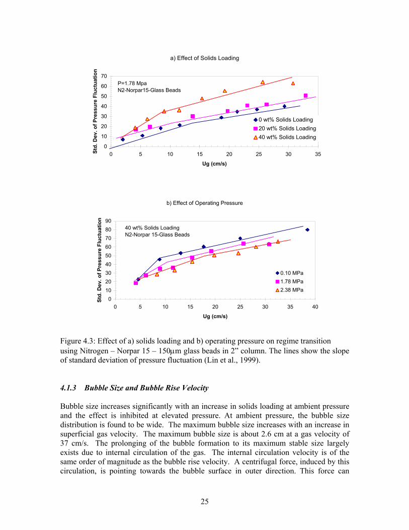
4.1 Hydrodynamics measurements in 2” column using DGD, ∆P Fluctuation, and Fiber Optic Probe This work has been carried out at Ohio State University. The liquid and gas phase used for these experiments are Norpar15 (density = 0.772 g/cc, viscosity =2.13 CPs, surface tension = 26.7 dynes/cm at ambient temperature and pressure) and nitrogen. The solid phase was glass beads of 150 µm. All the experiments have been operated in a batch liquid mode. The gas distributor is comprised of 19 triangular pitched holes of 0.45 mm diameter each and 0.156 % open area. The static liquid level is maintained at 50 cm above the distributor. 4.1.1 Overall gas holdup using DGD Dynamic Gas Disengagement (DGD) experiments have been performed to study the effect of operating pressure and solids loading on the overall gas holdup in 2” column. Figures 4.1 and 4.2 show the effect of pressure and solids loading on overall gas holdup. At low superficial gas velocities, the effect of operating pressure on the gas holdup is less compared to high superficial gas velocities. The influence of pressure has been found to be significant at higher superficial gas velocities. As can be seen in Figure 4.1, overall gas holdup is approximately double at 2.38 MPa relative to ambient pressure at superficial gas velocities higher than 20 cm/s. The presence of solids provides additional effects on the overall gas holdup. The gas holdup at high solids loading decreases considerably with an increase in pressure. The effect of addition of solids is less at low solids loading while it has been found to be significant at high solids loading, especially for liquid with high viscosity. Figure 4.2 summarizes the effect of solids loading on overall gas holdup at various isobaric conditions. The influence of solids loading on gas holdup is insignificant at ambient pressure while the significant effect is observed at high pressure. In general, overall gas holdup decreases with an increase in solids loading, particularly at high operating pressure. The presence of solids in three-phase system results in formation of larger bubbles due to increase in coalescence rate, which reduces overall gas holdup. Therefore, it can be concluded that an increase in operating pressure and decrease in the solids loading can improve the overall gas holdup. 4.1.2 Prediction of regime transition using ∆P fluctuations Figure 4.3 shows the effect of solids loading and operating pressure on the flow regime transition in 2” column using nitrogen-Norpar 15-glass beads (150 µm) system. The increase in pressure causes formation of smaller uniform sized bubbles, and hence the flow regime tends to be in homogeneous regime. This delays the regime transition. The addition of solids loading, on contrast, reduces transition velocity due to increase in pseudo-viscosity of slurry, which increases large bubble population.
22

Solids loading 0 % wt
0.00
0.10
0.20
0.30
0.40
0.50
0.60
0 5 10 15 20 25 30 35 40Ug, cm/s
Gas
Hol
dup
P= 0.10 MPaP= 1.78 MPaP= 2.38 MPa
Solids loading 20 % wt
0.00
0.10
0.20
0.30
0.40
0.50
0 10 20 30 40 50Ug, cm/s
Gas
Hol
dup
60
P= 0.10 MPaP= 1.78 MPaP= 2.38 MPa
Solids loading 40 %wt
0.000.050.100.150.200.250.300.350.40
0 10 20 30 40 50 6Ug, cm/s
Gas
Hol
dup
0
P= 0.10 MPaP= 1.78 MPaP= 2.38 MPa
Figure 4.1: Effect of pressure on overall gas holdup (Nitrogen - Norpar 15 - 150µm glass beads) at various solids loading
23

Pressure = 0.1 MPa
0.000.050.100.150.200.250.300.350.40
0 10 20 30 40 50 6Ug, cm/s
Gas
Hol
dup
0
εs = 0 %wtεs = 20%wεs = 40%wt
Pressure = 1.78 MPa
0.000.050.100.150.200.250.300.35
0 5 10 15 20 25 30 35
Ug, cm/s
Gas
Hol
dup
εs = 0 %wtεs = 20%wtεs = 40%wt
Pressure =2.38 MPa
0.00
0.10
0.20
0.30
0.40
0.50
0.60
0 5 10 15 20 25 30 35
Ug, cm/s
Gas
Hol
dup
εs = 0 %wtεs = 20%wtεs = 40%wt
Figure 4.2: Effect of solids loading on gas holdup (Nitrogen – Norpar 15 – 150µm glass beads) at various operating pressures
24
a) Effect of Solids Loading
0
10
20
30
40
50
60
70
0 5 10 15 20 25 30 35
Ug (cm/s)
Std.
Dev
. of P
ress
ure
Fluc
tuat
ion
0 wt% Solids Loading20 wt% Solids Loading40 wt% Solids Loading
P=1.78 MpaN2-Norpar15-Glass Beads
b) Effect of Operating Pressure
0102030405060708090
0 5 10 15 20 25 30 35 40
Ug (cm/s)
Std.
Dev
. of P
ress
ure
Fluc
tuat
ion
0.10 MPa1.78 MPa2.38 MPa
40 wt% Solids LoadingN2-Norpar 15-Glass Beads
Figure 4.3: Effect of a) solids loading and b) operating pressure on regime transition using Nitrogen – Norpar 15 – 150µm glass beads in 2” column. The lines show the slope of standard deviation of pressure fluctuation (Lin et al., 1999). 4.1.3 Bubble Size and Bubble Rise Velocity Bubble size increases significantly with an increase in solids loading at ambient pressure and the effect is inhibited at elevated pressure. At ambient pressure, the bubble size distribution is found to be wide. The maximum bubble size increases with an increase in superficial gas velocity. The maximum bubble size is about 2.6 cm at a gas velocity of 37 cm/s. The prolonging of the bubble formation to its maximum stable size largely exists due to internal circulation of the gas. The internal circulation velocity is of the same order of magnitude as the bubble rise velocity. A centrifugal force, induced by this circulation, is pointing towards the bubble surface in outer direction. This force can
25

suppress the disturbances at the gas-liquid interface and thereby stabilizing the interface. On other hand, the centrifugal force can also disintegrate the bubble as it increases with an increase in bubble size. The bubble breaks up when the centrifugal force exceeds the surface tension force, especially at high pressures where the gas density is high. A much smaller bubble size is observed at high pressure conditions compared with ambient pressure conditions, indicating that pressure has a significant effect on the breakage of the large bubbles. A narrower bubble size distribution is also observed under high pressure conditions. An increase in solids loading increases the maximum bubble size slightly. Figures 4.4 and 4.5 show the effects of pressure and solids loadings on bubble size and bubble rise velocity at superficial gas velocity of 30 cm/s and operating pressure of 1.78 MPa. The bubble rise velocity decreases with an increase in pressure for a given solids loading. In general, the addition of solids can reduce bubble rise velocity drastically. Further, due to the dominant role of the large bubbles in determining the gas holdup, the increase in bubble size due to the presence of particles explains the decrease in gas holdup as the solids loadings increases.
00.20.40.60.8
11.2
0.0-0.
1
0.2-0.
3
0.4-0.
5
0.6-0.
7
0.8-0.
9
1.0-1.
1
1.2-1.
3
1.4-1.
5
1.6-1.
7
1.8.-1
.9
2.0-2.
1
2.2-2.
3
2.4-2.
5
2.6-2.
7
2.8-2.
9
Bubble Chord Length, cm
PD
F
No solid
0
0.1
0.2
0.3
0.4
0.5
0.6
0.0-0.
1
0.2-0.
3
0.4-0.
5
0.6-0.
7
0.8-0.
9
1.0-1.
1
1.2-1.
3
1.4-1.
5
1.6-1.
7
1.8.-1
.9
2.0-2.
1
2.2-2.
3
2.4-2.
5
2.6-2.
7
2.8-2.
9
Bubble Chord Length, cm
40% Solid
Figure 4.4: Effect of solids loading on bubble size using Nitrogen - Norpar 15 - 150 µm glass beads in 2” column at Ug = 30 cm/s, P = 1.78 MPa
26

0
0.05
0.1
0.15
0.2
0.25
< 2.5
5.0-7.
5
10.0-
12.5
15.0-
17.5
20.0-
22.5
25.0-
27.5
30.0-
32.5
35.0-
37.5
40.0-
42.5
45.0-
47.5
50.0-
52.5
Bubble Velocity, cm/s
PD
FNo Solid
00.020.040.060.080.1
0.120.140.160.180.2
< 2.5
5.0-7.5
10.0-12
.5
15.0-17
.5
20.0-22
.5
25.0-27
.5
30.0-32
.5
35.0-37
.5
40.0-42
.5
45.0-47
.5
50.0-52
.5
Bubble Velocity, cm/s
40% solid
Figure 4.5: Effect of solids loading on bubble rise velocity using Nitrogen - Norpar 15 - 150 µm glass beads in 2” column at Ug = 30 cm/s, P = 1.78 MPa 4.2 Hydrodynamics Measurements in 6” column using CARPT and CT The three-phase holdups distribution presented in this section has been computed by the newly proposed CT/Overall gas holdup methodology. 4.2.1 Results of CT (gas holdup profile)/CARPT (solids axial velocity profile and turbulent parameters) Using Air-Water-Glass Beads System 4.2.1 a) Effect of Superficial Gas Velocity The reported literature suggests that an increase in superficial gas velocity increases the gas holdup and the liquid/solids velocity in both two- and three-phase bubble columns operated at atmospheric pressure (Degaleesan, 1997, Sannaes, 1997). The same effect of superficial gas velocity on radial gas holdup and solids velocity profiles at atmospheric pressure is observed in slurry bubble columns during this work. Figures 4.6 and 4.7
27

illustrate the effect of superficial gas velocity on radial gas holdup profiles and solids axial velocity profiles at atmospheric pressure, respectively. An increase in superficial gas velocity from 8 to 45 cm/s increases the centerline gas holdup from 0.3 to 0.55 while the centerline solids axial velocity increases from 24.59 to 48.21 cm/s. An increase in solids centerline axial velocity with an increase in superficial gas velocity is compensated with a larger negative axial velocity (–18.0 to –26.5 cm/s) at the wall, preserving the zero net solids flux. This results in an increase in the solids recirculation velocity in slurry bubble columns as the superficial gas velocity increases. The inversion point, where axial solids velocity becomes zero, occurs at φ0 = 0.65 – 0.70. It was found that, the inversion point shift slightly towards the center of the column with an increase in superficial gas velocity.
Gas holdup profile
0
0.1
0.2
0.3
0.4
0.5
0.6
0 0.2 0.4 0.6 0.8 1
r/R
gas
hold
up
Ug = 8 cm/sUg = 45 cm/s
Figure 4.6: Effect of superficial gas velocity on gas holdup profile (air-water-150 µm glass beads) in 6” column with 9.1 % vol. solids loading at 0.1 MPa
-30-20-10
0102030405060
0 0.2 0.4 0.6 0.8 1r/R
Uz
(cm
/s)
Ug = 8 cm/s
Ug = 45 cm/s
Figure 4.7: Effect of superficial gas velocity on solids axial velocity profile (air-water-150 µm glass beads) in 6” column with 9.1 % vol. solids loading at 0.1 MPa
28

The solids shear stress is proportional to the radial gradient of solids axial velocity. As there is an increase in solids axial velocity with an increase in superficial gas velocity (Figure 4.8), the shear stress should increase with an increase in superficial gas velocity. As shown in Figure 4.8, shear stress profiles exhibit maximum at r/R ≈ 0.5 while at the wall and in the center of the column, shear stress values are close to zero. This is in the agreement with the shear stress profiles in G-L systems (Degaleesan, 1997). The system becomes more turbulent with an increase in superficial gas velocity, which is reflected in an increased turbulent kinetic energy (TKE) (Figure 4.9) and eddy diffusivity profiles (Figure 4.10). Turbulent kinetic energy (TKE) profiles exhibit maximum values in the center of the column and decrease towards the column wall (Figure 4.9). The radial eddy diffusivity profiles (Drr) are qualitatively very similar to the shear stress profiles and exhibit maxima at r/R = 0.4 - 0.5 while at the wall and in the center of the column diffusivity values are close to zero. The magnitude of radial diffusivity (Drr) has been very low compared to axial diffusivity (Dzz) as shown in Figure 4.10. The axial eddy diffusivity profiles exhibit maxima close to the axial velocity inversion point at r/R ≈ 0.65 (Figure 4.10a). The centerline and the wall axial eddy diffusivities are typically between 50 and 80% of the maximum axial eddy diffusivity value.
Solids shear stress
0
100
200
300
400
0 0.2 0.4 0.6 0.8 1r/R
Trz
(cm
2/s2
) Ug = 8 cm/sUg = 45 cm/s
Figure 4.8: Effect of superficial gas velocity on solids shear stress profile (air-water-150 µm glass beads) in 6” column with 9.1 % vol. solids loading at 0.1 MPa
TKE
0
1000
2000
3000
4000
5000
6000
0 0.2 0.4 0.6 0.8 1
r/R
TKE
(cm
2/s2
)
Ug = 8 cm/sUg = 45 cm/s
Figure 4.9: Effect of superficial gas velocity on TKE (air-water-150 µm glass beads) in 6” column with 9.1 % vol. solids loading at 0.1 MPa
29

a) Solids axial diffusivity
0
100
200
300
400
500
0 0.2 0.4 0.6 0.8 1
r/R
Dzz
(cm
2/s2
)
Ug = 8 cm/sUg = 45 cm/s
b) Solids radial diffusivity
0
50
100
0 0.2 0.4 0.6 0.8 1
r/R
Drr
(cm
2/s2
)
8 cm/s45 cm/s
Figure 4.10: Effect of superficial gas velocity on a) solids axial diffusivity, and b) solids radial diffusivity (air-water-150 µm glass beads) in 6” column with 9.1 % vol. Solids loading at 0.1 MPa 4.2.1 b) Effect of Operating Pressure An increase in pressure increases bubble break-up rate, which results in generation of smaller bubbles and thereby increases gas holdup. Therefore, bubble column systems operated at higher pressures are characterized by larger gas holdup profiles (CREL Report, 2000a). The higher gas holdup and smaller size bubbles entrain the suspension of solids and liquid more effectively, which causes higher liquid and solids axial velocity profiles and therefore higher solids and liquid recirculation. This explanation has not been so far supported by experimental findings. However it is supported by the present CARPT solids velocity measurements in slurry systems and liquid velocity measurements in high pressure G-L bubble column systems. The effect of increased pressure that results in higher gas holdup and solids axial velocity profiles is illustrated in Figures 4.11 and 4.12. The comparison of the gas holdup and the solids axial velocity profiles at different conditions shows that, the effect of pressure on gas holdup and solids axial velocity profiles is as strong as the effect of superficial gas velocity. The shear stress is proportional to the radial gradient of axial velocity and therefore higher solids axial velocity profiles result in higher shear stress profiles. It has been shown that an increase in superficial gas velocity increases the solids axial velocity profiles and hence the shear stress (Figure 4.8). As an increase in pressure increases solids axial velocity, the higher shear stress profile has been observed at high pressure conditions (Figure 4.13). The comparison of Figures 4.8 and 4.13 leads to a conclusion that, the effect of pressure on the shear stress profiles is significantly smaller compared to the effect of superficial gas velocity. The shear stress profiles in high pressure systems are qualitatively similar to the profiles in systems operated at atmospheric pressure, with the maximum location at r/R ≈ 0.5.
30

Figure 4.14 shows the effect of operating pressure on TKE at superficial gas velocities of 8 and 45 cm/s. At 8 cm/s an increase in pressure decreases TKE in the center region. However, near the wall (i.e. r/R = 0.7 – 1) slight increase in TKE was observed. As superficial gas velocity increases to 45 cm/s, the region of higher TKE increases from r/R = 0.2 to 1. However, there is a decrease in TKE at higher pressure in the center region (~ 0 < r/R < 0.2). The effect of operating pressure on solids axial and radial diffusivities has been shown in Figure 4.15a and b. At 8 cm/s, an increase in pressure decreases axial diffusivity along the column radius. Near the wall region (r/R = 0.7 – 1) an increase in diffusivity at atmospheric pressure is found to be comparatively higher. However at 45 cm/s, an increase in pressure increases axial diffusivity up to r/R = 0.7 while a decrease in axial diffusivity at higher pressure was observed near the wall region (r/R = 0.7 – 1). The solids axial diffusivities show maxima around r/R = 0.7. The solids radial diffusivities are decreasing with an increase in operating pressure. It shows maxima between r/R = 0.4 – 0.5 while it decreases at the wall and near the center of the column. The effect of pressure was significant at 8 cm/s compared to 45 cm/s. However, the effect of operating pressure on turbulent parameters is less compared to the effect of superficial gas velocity. The findings are currently under further analysis to explain the above mentioned effects of operating pressure on turbulent parameters at low and high superficial gas velocities.
0
0.1
0.2
0.3
0.4
0.5
0.6
0 0.2 0.4 0.6 0.8 1
r/R
gas
hold
up
P = 0.1 MPaP = 0.4 MPa
Figure 4.11: Effect of operating pressure on gas holdup radial profile using air-water-150 µm glass beads in 6” column with 9.1 % vol. solids loading at 45 cm/s
-40
-20
0
20
40
60
80
0 0.2 0.4 0.6 0.8 1
r/R
Uz
(cm
/s)
0.1 MPa0.4 MPa
Figure 4.12: Effect of operating pressure on axial velocity profile using air-water-150 µm glass beads in 6” column with 9.1 % vol. solids loading at 45 cm/s
31

Solids shear stress
0100200300400500
0 0.2 0.4 0.6 0.8 1
r/R
Trz
(cm
2/s2
)
P = 0.1 MPaP = 0.4 MPa
Figure 4.13: Effect of operating pressure on solids shear stress profile using air-water-150 µm glass beads in 6” column with 9.1 % vol. solids loading at 45 cm/s
TKE
0100020003000400050006000
0 0.2 0.4 0.6 0.8 1
r/R
TKE
(cm
2/s2
)
Ug = 8 cm/s, P = 0.1 MPa
Ug = 8 cm/s, P = 0.4 MPa
Ug = 45 cm/s, P = 0.1MPa
Ug = 45 cm/s, P = 0.4MPa
Figure 4.14: Effect of operating pressure on solids TKE using air-water-150 µm glass beads in 6” column with 9.1 % vol. solids loading at 8 and 45 cm/s
a) Solids axial diffusivity
0100200300400500600
0 0.2 0.4 0.6 0.8 1
r/R
Dzz
(cm
2/s2
)
Ug = 8 cm/s, P = 0.1MPa
Ug = 8 cm/s, P = 0.4MPa
Ug = 45 cm/s, P = 0.1MPa
Ug = 45 cm/s, P= 0.4MPa
32

b) Solids radial diffusivity
0
50
100
0 0.2 0.4 0.6 0.8 1r/R
Drr
(cm
2/s2
)
Ug = 8 cm/s, P = 0.1 MPa
Ug = 8 cm/s, P = 0.4 MPa
Ug = 45 cm/s, P = 0.1 MPa
Ug = 45 cm/s, P = 0.4 MPa
Figure 4.15: Effect of operating pressure on a) solids axial diffusivity profile b) solids radial diffusivity profile using air-water-150 µm glass beads in 6” column with 9.1 % vol. solids loading at 8 and 45 cm/s 4.2.2 Results of CT (gas and solids holdup profile) Using Air-Therminol LT-Glass Beads System 4.2.2 a) Effect of Superficial Gas Velocity: The effect of superficial gas velocity on gas holdup and solids holdup is shown in Figures 4.16a and b. Due to increase in overall gas holdup with superficial gas velocity, the magnitude of gas holdup profile also increases and the system tends to get into churn-turbulent flow regime with increase in superficial gas velocity. The effect of superficial gas velocity on solids holdup profile is not much significant as compared to gas holdup, which would be due to the assumption of uniform cross-sectional solids loading in the CT/Overall gas holdup data reconstruction methodology discussed earlier in section 3.6. However, in the center region of the column (~ 0 ≤ r/R ≤ 0.5), solids holdup decreases slightly with the increase in superficial gas velocity, whereas at the wall region, the effect of superficial gas velocity diminishes. 4.2.2 b) Effect of Operating Pressure: The effect of operating pressure on gas holdup and solids holdup profiles at superficial gas velocity of 14 cm/s is shown in Figures 4.17a and b. With an increase in pressure, the break up rate increases while coalescence rate decreases which leads to smaller bubble sizes and subsequently into an increase in gas holdup (Wilkinson, 1993). This results in higher gas holdup profile with an increase in operating pressure at the same superficial gas velocity. The solids holdup profile decreases with an increase in pressure. The effect of pressure on solids holdup profile is found to be less significant compared to the gas holdup profile.
33

a)
0
0.1
0.2
0.3
0.4
0.5
0.6
0 0.2 0.4 0.6 0.8 1
r/R
gas
hold
upUg = 14 cm/sUg = 8 cm/s
b)
0
0.1
0.2
0.3
0 0.2 0.4 0.6 0.8 1
r/R
solid
s ho
ldup
Ug = 14 cm/sUg = 8 cm/s
Figure 4.16: Effect of superficial gas velocity on a) gas holdup, and b) solids holdup profile (air – Therminol LT-150 µm glass beads) in 6” column with 9.1 % vol. solids loading at 0.1 MPa.
34

a)
00.10.20.30.40.50.6
0 0.2 0.4 0.6 0.8 1
r/R
gas
hold
upP = 0.1 MPaP = 1 MPa
b)
0
0.1
0.2
0.3
0.4
0 0.2 0.4 0.6 0.8 1
r/R
solid
s ho
ldup
P = 0.1 MPaP = 1MPa
Figure 4.17: Effect of operating pressure on a) gas holdup, and b) solids holdup profile (air– Therminol LT-150 µm glass beads) in 6” column with 9.1 % vol. solids loading at 14 cm/s.
35

5. DEVELOPMENT OF ARTIFICIAL NEURAL NETWORK CORRELATION FOR PREDICTION OF OVERALL GAS HOLDUP IN BUBBLE COLUMNS
In attempt to improve the design and scale-up of bubble columns, a correlation has been proposed to predict overall gas holdup in bubble columns (Shaikh and Al-Dahhan, 2002a, 2002b). This correlation has been developed with the aid of Artificial Neural Network and Dimensional Analysis, and can be useful over a wide range of operating and design conditions. The details of the developed correlation are described in Appendix A as full manuscript submitted to Chemical Engineering and Processing (Shaikh and Al-Dahhan, 2002).
36

6. NOMENCLATURE AND REFERENCES
6.1 NOMENCLATURE ∆h vertical distance between two tips, cm ∆P Pressure drop A Absorbance D Column diameter, m Drr solids radial diffusivity, (cm/s)2 Dzz solids axial diffusivity, (cm/s)2
g gravitational constant, m/s2
H Column height, m I,I0 intensity of radiation received by detector and emitted by the source l bubble chord length, cm ns radioactive particle occurences P Pressure inside column, psi R radius of column, in r/R Dimensionless radius RK relative volumetric coefficient T column temperature, 0C t time, seconds Trz solids shear stress, (cm/s)2 U Axial liquid velocity, cm/s ub bubble rise velocity, cm/s Ug Superficial gas velocity, cm/s Ur Radial velocity of solids, cm/s Uz Axial velocity of solids, cm/s z column height Greek letters
Sν cross sectional solids loading
Gε cross-sectional average gas hold up
Sε solids holdup τ time period when bubble is in contact with lower tip of probe, sec ρg Gas density, gm/cc
Lρ Liquid density, gm/cc
Lσ Liquid surface tension, dynes/cm
Lµ Liquid viscosity, cPs ρµ volumetric attenuation coefficient
37

6.2 REFERENCES Badgujar, M. N., Deimling, A., Morsi, B. I., Shah, Y. T. and Carr, N. L. (1986). Solids distribution in a batch bubble column. Chem. Eng. Commun., 48, 127 CREL (2000a). Engineering development of slurry bubble column reactor (SBCR) technology. 22th Quarterly report for the Department of Energy contract No. DE-FC22-95PC95051, Washington University, St. Louis, MO. CREL (2000b). Engineering development of slurry bubble column reactor (SBCR) technology. 23rd Quarterly report for the Department of Energy contract No. DE-FC22-95PC95051, Washington University, St. Louis, MO. Deckwer W.-D and A. Schumple, Improved tools for bubble column reactors design and scale up, Chem. Eng. Sci., 48, 889-911, 1993.
Degaleesan, S., Turbulence and liquid mixing in bubble columns, D.Sc. Thesis, Washington University, St. Louis, MO, 1997.
Devanathan, N. Investigation of liquid hydrodynamics in bubble columns via computer automated radioactive particle tracking (CARPT). D.Sc Thesis, Washington University, St. Louis, 1991. Fan, L.-S., Gas-liquid-solid fluidization engineering, Butterworths Series in Chemical Engineering, Boston, 1989.
Kondukov, N. B., Kornilaev, A. N., Skachko, I. M., Akhromenkov, A. A. and Kurglov, A. S. (1964). An invetsigation of the parameters of moving particles in a fluidized bed by a radioisotopic method. Int. Chem. Eng., 4, 43.
Kumar, S.B., Computed tomography measurements of void fraction and modeling of the flow in bubble columns, Ph.D. Thesis, Florida Atlantic University, Boca Raton, 1994. Limtrakul, S. (1996). Hydrodynamics of liquid fluidized beds and gas-liquid fluidized beds. D.Sc. Thesis, Washington University, St. Louis, MO.
Lin, T.-J., Tsuchiya, K. and Fan, L.-S. (1998). Bubble flow characteristics in bubble columns at elevated pressure and temperature, AIChE J., 44, 545.
Lin, T.-J., Tsuchiya, K., and Fan, L.-S. (1999). "On the measurements of regime transition in high-pressure bubble columns", Can. J. of Chem. Eng., 77, 370- 374. Luo, X., Lee, D. J., Lau, R., Yang, G. and Fan, L.-S. (1999). Maximum stable bubble size and gas holdup in high pressure slurry bubble columns. AIChE J., 45, 665.
38

Matsumoto, T., Hidaka, N., Gushi, H. and Morooka, S. (1992). Axial segregation of multicomponent solid particles suspended in bubble columns. Ind. Eng. Chem. Res., 31, 1562.
Moslemian, D., Devanathan, N. and Dudukovic, M. P. (1992). Radioactive particle tracking technique for investigation of phase recirculation and turbulence in multiphase systems. Rev. Sci. Instrum., 63, 4361 Rados, N., Slurry bubble column hydrodynamics, D.Sc. Thesis, Washington University, St. Louis, 2002. Rajamani Krishna, Jeroen W. A. de Swart, Jurg Ellenberger, Gilbert B. Martina, Cristina Maretto ‘Gas Holdup in Slurry Bubble Columns: Effect of column diameter and slurry concentrations,’ AIChE J., 43, 2, 311-316, 1997. Sannaes B. H. (1997). Solids movement and concentration profiles in column slurry reactors. Dr. Ing. Thesis, Norwegian University of Science and Technology, Trondheim, Norway.
Shaikh, A., Al-Dahhan M.H., Development of Neural Network based Correlation for Overall Gas Holdup in Bubble Column Reactors, Chem. Eng. Proc., 2002 (submitted). Shaikh, A., Al-Dahhan, M.H., Prediction of Overall Gas Holdup in Bubble Column Reactors via Artificial Neural Network Correlation, Paper 114c Presented at AIChE Spring Meeting, New Orleans, LA, March 10-14, 2002a. Shaikh, A., Al-Dahhan, M.H., Development of neural network based correlation for prediction of overall gas holdup in bubble column reactors, Paper 0608, Presented at ISCRE 17, Hong Kong, China, August 25 – 28, 2002b. Wilkinson, P. M. (1991). Physical aspects and scale-up of high pressure bubble columns. Ph.D. Thesis, Rijksuniversiteit Groningen, Netherlands.
Wilkinson, P. M., van Schayk, A., Spronken, J. P. M. and van Dierendonck, L. L. (1993). The influence of gas density and liquid properties on bubble breakup. Chem. Eng. Sci., 48, 1213.
39

APPENDIX A
DEVELOPMENT OF ARTIFICIAL NEURAL NETWORK CORRELATION
for PREDICTION OF OVERALL GAS
HOLDUP in
BUBBLE COLUMNS
40

Development of An Artificial Neural Network Correlation for
Prediction of Overall Gas Holdup in Bubble Column Reactors
Ashfaq Shaikh, Muthanna Al-Dahhan*
Chemical Reaction Engineering Laboratory, Department of Chemical Engineering,
Campus Box 1198, 1 Brookings Drive, Washington University, St. Louis, MO 63130-
4899 USA
Abstract
In the literature, several correlations have been proposed for gas holdup prediction in
bubble columns. However, these correlations fail to predict gas holdup over a wide range
of conditions. Based on a databank of around 5500 measurements collected from the
open literature, a correlation for gas holdup was derived using a combination of
Dimensional Analysis and Artificial Neural Network (ANN) modeling. The overall gas
holdup was found to be a function of four dimensionless groups: Reg, Frg, Eo/Mo, and
Lg ρρ / . Statistical analysis showed that the proposed correlation has an average absolute
relative error (AARE) of 10 % and a standard deviation of 11 %. A comparison with
selected correlations in the literature showed that the developed ANN correlation
noticeably improved prediction of overall gas holdup. The developed correlation also
shows better prediction over a wide range of operating conditions, physical properties,
and column diameters, and it predicts properly the trend of the effect of the operating and
design parameters on overall gas holdup.
Key Words: force analysis, artificial neural network, gas holdup, database, statistical
analysis
*Corresponding author Tel. 314-935-7187. E-mail [email protected]
41

Introduction
Bubble columns are two-phase gas-liquid systems in which gas is dispersed through a
sparger and bubbles through a liquid in vertical cylindrical columns, with or without
internals. Bubble columns are widely used in chemical, petrochemical, biochemical and
metallurgical industries as multiphase reactors and contactors. Examples of such
chemical and petrochemical processes are partial oxidation of ethylene to acetaldehyde,
wet-air oxidation (Deckwer, 1992), methanol synthesis, Fischer-Tropsch synthesis
(Wender, 1996), and hydrogenation of organic liquids. In biochemical industries, bubble
columns are used for cultivation of bacteria, cultivation of mold fungi (Lehmann et al.,
1978), and treatment of sewage (Diesterweg, 1978). In metallurgical industries, it can be
used for leaching of ores.
The advantages of bubble column include good heat and mass transfer characteristics, no
moving parts and thus reduced wear and tear, higher catalyst durability, ease of operation,
compactness and low operating and maintenance. Bubble columns are an attractive
reactor for various multiphase processes, especially for processes involving highly
exothermic reactions. These reactors are operated in semi-batch or continuous mode, with
low superficial liquid velocities compared to gas velocities. For this reason, the
hydrodynamics of such reactors are controlled mainly by the gas flow. In spite of the
simplicity of the mechanical design of bubble columns, their fluid dynamics are complex.
Therefore, due to complex interactions among the flowing phases, a proper understanding
of hydrodynamics and transport parameters to enable reliable design and scale-up is still
lacking.
Overall gas holdup is one of the important parameters for bubble column design and
scale-up. It is defined as the fraction of the reactor dynamic volume occupied by the gas.
Gas holdup and its radial profile govern liquid recirculation, flow pattern, mixing, and
heat and mass transfer in bubble column reactors. Two types of regimes are encountered
in bubble column operation, viz., homogeneous (bubbly) and heterogeneous (churn-
turbulent) flow regimes (Kastanek et al., 1993). An adequate knowledge of overall gas
42

holdup and its profile are needed for flow regime identification as well as for modeling,
design, and scale-up of bubble column reactors.
Over the years, overall gas holdup has been studied extensively with various
measurement techniques, ranging from measuring the change in dynamic height or
measuring conventional pressure drop to computed tomography. In the literature,
numerous correlations have been proposed for overall gas holdup. Some of the more
important correlations are listed in Table 1. Kemoun et al. (2001) compared gas holdup
predicted by various correlations with the cross-sectional averaged gas holdup measured
using Computed Tomography (CT) in the fully developed region at atmospheric to high
pressure and at low to high superficial gas velocities. The comparison between their
experimental data and predicted gas holdups from various correlations at atmospheric and
high pressure (0.7 MPa) is shown in Fig.1 and 2. The findings can be summarized as
follows,
At atmospheric pressure, the correlation of Idogawa et al. (1985) gives the best
agreement with the CT experimental data, except at UG = 5 cm/s.
At higher pressures and over the entire superficial gas velocity range studied, the
correlation of Hammer et al. (1984) gives better prediction, followed by Wilkinson et
al. (1992) and Idogawa et al. (1987).
At higher pressures and higher superficial gas velocity (UG = 10 cm/s), the correlation
of Krishna et al. (1996) and Luo et al. (1999) also provides reasonable prediction of
gas holdup.
While several correlations give reasonable predictions at different conditions, Kemoun et
al. (2001) did not find any correlation that consistently predicted their experimental data
at the studied operating conditions. To facilitate the scale-up of bubble columns, there is a
need for a correlation that can predict overall gas holdup over a range of operating
conditions, physical properties, and column dimensions.
Since the early 80’s, artificial neural networks have been used extensively in chemical
engineering for such various applications as adaptive control, model based control,
process monitoring, fault detection, dynamic modeling, and parameter estimation (Bhat,
et al., 1990). The artificial neural network provides a nonlinear mapping between input
43

and output variables and is also useful in providing cross-correlation among these
variables. The mapping is performed by the use of processing elements and connection
weights. The Neural Network is a useful tool in rapid predictions such as steady-state or
transient process flow sheet simulations, on-line process optimization and visualization,
and parameter estimation. In multiphase reactor research, there have been efforts to apply
neural networks for improved prediction of design and scale-up variables. Cai et al.
(1994) applied Kohonen self-organizing neural networks to identify flow regimes in
horizontal air-water flow. Leib et al. (1995) used a neural network model along with the
mixed-cell model to predict slurry bubble column performance for the Fischer-Tropsch
synthesis. Bensetiti et al. (1997), Larachi et al. (1998), Piche et al. (2001), and Illiuta et
al. (2002) used an Artificial Neural Network (ANN) to improve the prediction of various
hydrodynamic parameters in packed bed and fluidized bed reactors.
Building on these studies, the focus of this work is to develop a unified correlation for
overall gas holdup prediction in bubble columns which can be useful for design
engineers. To develop such a correlation, an approach that combines both an Artificial
Neural Network (ANN) and Dimensional Analysis has been used. The correlation has
been derived from a broad experimental data bank collected from the open literature
(5500 measurements covering a wide range of column dimensions and physical
properties).
Artificial Neural Network Modeling
Neural Networks are computer algorithms inspired by the way information is processed
in the nervous system. An Artificial Neural Network is a massively parallel distributed
processor that has a natural propensity for storing experimental knowledge and making it
available (Ripley, 1996). An important difference between neural networks and standard
Information Technology (IT) solutions is their ability to learn. This learning property has
yielded a new generation of algorithms that can
- learn from the past to predict the future
44

- extract rules for reasoning in complex environments
- offer solutions when explicit algorithms and models are unavailable or too
cumbersome.
Artificial Neural Networks emulates biological nervous systems and adaptive biological
learning. An ANN paradigm is composed of a large number of highly interconnected
processing elements, analogous to neurons, that are tied together with weighted
connections that are analogous to synapses. Learning in biological systems involves
adjustments to the synaptic connections between the neurons. This is true of ANNs as
well. Learning typically occurs through training or exposure to a truth set of input/output
data where the training algorithm iteratively adjusts the connection weights. These
connection weights represents the knowledge necessary to solve specific problems.
ANNs are being applied to an increasing number of real-world problems of considerable
complexity. They are good pattern recognition engines and robust classifiers, with the
ability to generalize in making decisions about imprecise input data. They offer ideal
solutions to a variety of classification problems such as speech, character, and signal
recognition, as well as prediction and system modeling where the physical processes are
not understood or are highly complex. The advantage of ANNs lies in their resilience
against distortions in the input data and their learning capability. They are often good at
solving problems that are too complex for conventional technologies, such as problems
that do not have an algorithmic solution or for which an algorithmic solution is too
complex to be found.
There are multitudes of different types of ANNs. Some of the more popular include the
multilayer perceptron, which is generally trained with the backpropagation of error
algorithm, the Hopfield ANN, and the Kohonen ANN. Some ANNs are classified as
feedforward, while others are recurrent, depending on how data is processed through the
network. Another way of classifying ANN types is by their method of learning, as some
ANNs employ supervised training, while others are referred to as unsupervised or self-
organizing (Ripley, 1996).
45

In this work, a multilayer neural network has been used, as it is effective in finding
complex non-linear relationships. It has been reported that multilayer ANN models with
only one hidden layer are universal approximators (Hornik et al., 1989). Hence, a three-
layer feedforward neural network is chosen as a regression model. The weighting
coefficients of the neural network are calculated using the special-purpose software
NNFit (Cloutier et al.,1996). NNFit is a non-linear regression software that discloses
relationships between a set of normalized input variables, Ui, and a set of normalized
output variable, Sk. Figure 3 shows the transformation S = f (U) using a neural network
with a single hidden layer. The transformation of actual variables (X, Y) to normalized
variables (U, S) is given by (Cloutier et al., 1996),
(1) )/log( X)/log(
minmax
min
XXXU i
i =
)/log()/log(
minmax
min
YYYYS k
k =
(2)
where, Xi and Yk are raw input and output variables. The basic structure of this type of
neural network is described by the following set of equations. The various layers are
interconnected to each other by a sigmoid function through the fitted parameters wij, wjk
in the following manner,
∑−+= +
=
1
1]exp[1
1J
jjjk
kHw
S
and (3)
46

∑−+= +
=
1
1]exp[1
1I
iiij
jUw
H
(4)
where I,J,K indicate the input, hidden and output nodes of the ANN structure,
respectively. HJ+1 and UI+1 (Figure 3) are the bias constants which are set equal to one. wij
and wjk are weighting parameters which are fitted by the NNFit regression model, using a
quadratic criterion as a minimization algorithm, a quasi-Newton method of the BGFS
type (Broyden-Fletcher-Goldfrab-Shanno) (Cloutier et al., 1996).
Development of the ANN based correlation
The development of the ANN-based correlation began with the collection of a large
databank. The physical parameters were then subjected to force analysis in order to
maintain dimensional homogeneity. The last step was to perform a neural regression, and
to validate it statistically.
Collection of data
As mentioned earlier, over the years researchers have amply quantified the
hydrodynamics of bubble column reactors based on the overall gas holdup. In this work,
about 5500 experimental points have been collected from 60 sources spanning the years
1965 to 2000. This wide range of database includes experimental information from
different physical systems to provide a unified correlation for overall gas holdup. Table 2
suggests the wide range of the collected databank for gas holdup.
Most of the hydrodynamic studies on bubble columns were performed using air-water
systems. To assess the impact of physical properties such as density, surface tension, and
viscosity, several other gas-liquid systems were included in the database. Bubble columns
are generally operated with low liquid velocities, which have been reported to have little
or no effect on overall gas holdup (Kelkar et al., 1983, Shetty et al., 1992). Hence, in this
47

work we have considered data only for columns with liquid in batch mode and gas in
continuous mode. As industrial conditions of interest are at high pressure, we have added
experimental studies at high pressures up to 2 MPa. Since reactor scale-up extends small
diameter behavior to large diameters, and in order to make the developed correlation
industrially useful, we have included data obtained up to 5.5 m column diameter, the
largest diameter described in the open literature. All the data was collected for cylindrical
columns, as they are the favored geometry in a majority of industrial applications. Since
the data was collected from wide range of sources, there is no uniformity in the
measurement techniques of gas holdup. The techniques range from measurement by level
change, or pressure drop up to densitometry and computed tomography.
Force Analysis
The force analysis checked whether the physical parameters in the database can be
formulated in a dimensionally homogeneous manner or not. It consists of two steps
i) All physical parameters that influence overall gas holdup are put in a so called
“wish-list”.
ii) The dimensional homogeneity of the physical parameters was checked by
transforming them into various forces.
Based on the extensive literature review, the following input variables have been found to
affect gas holdup
i) Superficial gas velocity: Gas holdup increases with an increase in superficial gas
velocity. The effect is relatively weaker in the churn-turbulent regime.
ii) Column Diameter: Gas holdup decreases with an increase in column diameter.
Many researchers have claimed that above 15 cm, the effect of column diameter is
negligible (Botton, 1978, Wilkinson, 1991).
48

iii) Operating Pressure: An increase in pressure increases gas density and decreases the
mean bubble size and the population of large bubbles, thus increasing gas holdup
(Wilkinson 1991, Smith et al., 1995).
iv) Liquid physical properties: An increase in density and a decrease in surface tension
and viscosity both increase gas holdup (Wilkinson , 1991).
v) Sparger Design: The effect of the sparger is influential in the homogeneous regime
(Kelkar et al., 1983).
Once the crucial identification of raw variables has been performed, the input variables
were then converted into various physical forces. Some of the important forces are
a) gas inertial force: 2GGuρ
b) gas viscous force: G duG /µ
c) liquid gravitational force: gdLρ
d) gas gravitational force: gdGρ
e) capillary force: L / dσ
Dimensionless numbers were then formed by taking ratios of various physical forces
which are determined from the input variables. In addition to this, the various
dimensionless groups used in the gas holdup correlations reported in literature were
considered. Then, on the basis of the observed effect of some parameters on the overall
gas holdup, some of the dimensionless groups such as ratios of densities, etc., were
added.
The main advantage of performing dimensional analysis is to reduce the number of input
parameters, i.e., there are fewer dimensionless input groups than the raw parameters. The
other advantage of dimensional analysis lies in the “scale-invariant” property of a
dimensionless frame. The “scale-invariance” makes dimensional analysis a primary step
in scale-up of reactors (Zlokarnik, 1998).
49

Neural Regression
Force analysis is used to produce dimensionless groups in this case, but it alone can not
determine which groups are relevant and should be used as input. Therefore, we used the
following methodology to select the most pertinent inputs (Bensetiti et al., 1997).
Out of the number of dimensionless groups derived, we used ANN regression to establish
the best set of chosen dimensionless groups, which describes overall gas holdup
(Bensetiti et al., 1997, Larachi et al., 1998). The following criteria guide the choice of the
set of input dimensionless groups:
- The dimensionless groups should be as few as possible,
- Each group should be highly cross-correlated to the output parameter,
- These input groups should be weakly cross-correlated to each other,
- The selected input set should give the best output prediction, which is checked by
using statistical analysis [e.g., average absolute relative error (AARE), standard
deviation, cross-correlation coefficient].
- There should be minimum complexity in neural network architecture, i.e., a
minimum number of hidden layers J.
While choosing the most expressive dimensionless groups, there is a compromise
between the number of dimensionless groups and prediction. The main concern with the
number of dimensionless groups is due to two reasons: first, there should be fewer
expressive groups than raw parameters, and second for feasible scale-up we may need a
minimum number of dimensionless groups.
The cross-correlation analysis which signifies the strength of the linear relation between
input and output is then used to find the dependence between input and output groups. A
number of inputs can be highly cross-correlated to output, but there should not be any
dependency between these groups; otherwise, it just adds to the complexity of the
50

structure rather than contributing significantly to improve the quality of the network. One
should be careful here: although the cross-correlation analysis reveals the dependence
between inputs and outputs, it also hides non-monotonic relationships. This can result
into losing an important dimensionless group. Therefore in this study, several sets of
input groups were made and tested via rigorous trial-and-error on the Artificial Neural
Network. The above mentioned criteria were then used to identify the most pertinent set
of input groups.
The statistical analysis of prediction is based on the following criteria:
The average absolute relative error (AARE) should be minimum.
∑−
=N
erimental
erimentalpredicted
yyy
NAARE
1 exp
exp1
The standard deviation should be minimum.
∑= −
−−
=N
i
ierimental
ierimentalipredictedl
N
AAREy
yy
1
2
)(exp
)(exp)(
1
)(
σ
The cross-correlation coefficient, R between input and output should be around
unity
∑∑
∑
==
=
−−
−−=
N
imeanpredictedipredicted
N
imeanerimentalierimental
meanpredictedipredicted
N
imeanerimentalierimental
yyyy
yyyyR
1
2)()(
1
2)(exp)(exp
)()(1
)(exp)(exp
)()(
))((
51

Neural networks often encounter the well-known ‘overfitting’ problem, which can make
use of the ANN unreliable. To avoid ‘overfitting’ and make the ANN more useful, the
following approach was used. The whole database was split into two parts, learning and
generalization. The first part, called the ‘learning file’, was used to perform minimization
using the ANN. The remaining part, called the ‘generalization file’, was used to validate
the model. Following the common practice, the learning file was made by randomly
selecting about 70% of the database to train the network. The remaining 30% of data was
then used to check the generalization capability of the model. The hidden layers, J, and
fitting parameters wij and wjk are a priori unknown. The number of hidden layers was
varied and chosen empirically according to the above criteria. The weighting parameters
were then determined by non-linear least-square regression over known random
inputs/outputs (70% of the data, which was picked randomly). The remaining 30% of the
database was utilized for validation of predicted weighting parameters. The chosen set of
inputs must show the best prediction during training and generalization, i.e., show the
least error on both learning and generalization files.
Results
After collecting the large databank, we subjected it to dimensional analysis, which
resulted into hundreds of dimensionless groups. As a matter of fact, using all these groups
is not feasible. Hence, to make the use of the developed model feasible, after forming a
number of sets of dimensionless groups, cross-correlation analysis was performed. As the
cross-correlation analysis can hide non-monotic relationships, rigorous trial-and-error
testing with the aid of ANN was also performed. The criteria mentioned above led to four
pertinent input dimensionless groups: Reg, Frg, Eo/Mo, and Lg ρρ / . The ratio of the
densities of the gas and liquid was added to account for the effect of high pressure. This
particular set of dimensionless groups showed consistent performance on both the
learning and generalization file. The sets of dimensionless groups which did not show
consistent performance were omitted, despite their remarkable performance on the
learning file. Table 3 lists the most expressive input groups and is accompanied by the set
of equations and weighting parameters. To use the ANN correlation, these equations and
52

parameters can be readily put in a spreadsheet file for overall gas holdup calculations in
bubble column reactors. They will also be available later on our website.
Figure 4 shows the parity plot of the experimental and predicted overall gas holdup using
the ANN correlation on the whole database. The ANN predicts the overall gas holdup
with an AARE of 10 %. For comparison, Figure 5 is the parity plot of the experimental
and predicted overall gas holdup, based on the whole database and using selected
literature correlations along with the ANN correlation. In this case, the correlations were
selected based on the conclusions of Kemoun et al., (2001). From the figure, it is clear
that the ANN correlation predicts overall gas holdup better than these two correlations.
Moreover, Table 4 compares an additional important correlations in literature on the basis
of statistical analysis, and confirms that the ANN performs better than they do.
Table 5 shows the statistical parameters for some of the input sets of the ANN considered
in this analysis. It includes different numbers of hidden layers to justify the selection of
the current input set.
ANN correlation prediction of gas holdup using different liquids
The major portion of the databank consists of water as the liquid phase, since most of the
reported studies used water for simplicity and economy. As mentioned earlier, the
databank has a wide range of fluid physical properties, therefore we have performed
statistical analysis on fluids with different physical properties to check whether the ANN
correlation predicts overall gas holdup consistently or not. Figure 6 shows the parity plot
of the experimental and predicted gas holdup using the ANN correlation for water at
different operating conditions, while Table 6 shows the statistical analysis of the gas
holdup predictions for different fluids, along with their physical properties. It is obvious
that the ANN correlation predicts satisfactorily the effect of liquid physical properties on
the overall gas holdup.
53

ANN correlation prediction of gas holdup at different pressures
In the literature, there are many correlations proposed for prediction of overall gas holdup
at atmospheric pressure, and there are some correlations developed at high pressure as
well. As mentioned by Kemoun et al., (2001), some of these correlations show good
prediction of overall gas holdup at atmospheric pressure but fail at high pressures.
Although we have included data up to 2 MPa, the major part of the databank is of gas
holdup at atmospheric pressures. Therefore, we have separated data of different pressures
and performed statistical analysis to check how well the ANN predicts gas holdup at
varied pressures. Such statistical evaluation is shown in Table 7, and it is obvious that the
developed ANN correlation predicts well the overall gas holdup at both elevated
atmospheric pressures.
ANN correlation prediction of gas holdup for different column diameters
The agreement between predicted and experimental gas holdup for different column
diameters has been evaluated by the statistical analysis shown in Table 8. The ANN
consistently predicts gas holdup over a wide range of diameters within acceptable error.
ANN Correlation Prediction of the Trend of the Effect of Different Parameters
In this part of the work, we checked how well the prediction of the developed ANN
correlation captures the reported trend of the effect of different parameters on the overall
gas holdup.
Effect of Column Diameter
Figure 7 shows a comparison between the predictions obtained using the ANN
correlation and experimental data for air-water systems at ambient conditions in different
columns (d = 0.05,0.15, 0.3 m) at different superficial gas velocities. The trend shown by
the ANN correlation is in agreement with published literature.
54

Effect of Operating Pressure
Figure 8 shows a comparison between the predictions obtained using the ANN
correlation and experimental data for a nitrogen-water system in a 0.15 m diameter
column at different operating pressures (P = 0.1, 0.6, 1.2 MPa). It shows an increase in
gas holdup with an increase in pressure, as reported in the literature (Wilkinson 1995).
Effect of Liquid Physical Properties
To check the effect of liquid properties, ANN correlation simulations were carried out at
the experimental conditions of Reilly et al. (1994) and Vermeer et al. (1981), with the
results shown in Figure 9. This particular data from Reilly et al. (1994) and Vermeer et
al. (1981) was not included in the database used for training and validation of the
developed ANN correlation.
To compare the predictions with the Reilly et al. (1994), a simulation was carried out at
ambient conditions with ISOPAR G* (ρL = 740 kg.m-3, µL = 0.861 mPa.s, σL = 0.0235
N.m-1) – CO2 (ρG = 1.84 kg.m-3) in 15 cm diameter column. Similarly, to compare the
predictions with the Vermeer et al. (1981), a simulation was carried out at ambient
conditions in 19 cm column with Turpentine (ρL = 761 kg.m-3, µL = 0.00094 Pa.s, σL =
0.024 N.m-1) – N2 (ρG = 1.146 kg.m-3). The predictions are in good agreement with the
experimental data, particularly in the bubbly flow regime (uG < 3 cm/s). However, in the
transition region (uG = 3 – 5 cm/s) and churn-turbulent flow regime (uG ≥ 5 cm/s), there is
some deviation between the experimental data of Reilly et al. (1994) and the ANN
correlation prediction, although the difference is within 11% AARE. This agreement
suggests that grouping the data for different flow regime and having a correlation for
each flow regimes would benefit the accuracy of the prediction. This approach is being
considered for future evaluation.
Overall, the simulations performed using the ANN correlation predict the effect of
different parameters on overall gas holdup per the trend reported in the literature. They
prove its utility as a design estimation tool for bubble column reactors.
55

Conclusions
Compared to the selected literature correlations, the Artificial Neural Network correlation
shows noticeable improvement in the prediction of overall gas holdup. The neural
network correlation yields an AARE of 10%, with a standard deviation of 11%, which is
better than those obtained for the selected literature correlations. This work identified
Reg, Frg, Eo/Mo, and Lg ρρ / as expressive dimensionless groups to predict overall gas
holdup. Also, the ANN correlation yielded improved predictions for a variety of liquids, a
wide range of operating pressures, and various column diameters. In addition, the
developed correlation captures properly the trend of the effect of various operating and
design parameters on the overall gas holdup reported in the literature. Hence the
developed ANN correlation should be useful in the scale-up of bubble column reactors.
Acknowledgements
The authors are thankful for the UCR-DOE grant (DE-FG-26-99FT40594) which made
this work possible. The authors also gratefully acknowledge the help extended by David
Newton (an undergraduate student) during the data collection. The encouragement and
the support received from Prof. M. P. Dudukovic during the course of this work have
been invaluable.
Nomenclature
d column diameter, m
DR ratio of gas and liquid phase densities, dimensionless
Eo Etovos number, dimensionless
Frg gas Froude number, dimensionless
g gravitational constant, m s-2
I number of input nodes
J number of hidden layers
56

K number of output layers
Mo liquid Morton number, dimensionless
N number of data points
R cross-correlation coefficient
Sk normalized output variable
ug superficial gas velocity, m s-1
Ui normalized input variable
wij,wjk ANN fitting parameters
Greek letters
σ standard deviation
ρg gas phase density, kg m-3
ρL liquid phase density, kg m-3
σL liquid surface tension, N m-1
µL liquid viscosity, kg m-1 s-1
εG overall gas holdup, dimensionless
Abbrevations
AARE average absolute relative error
ANN artificial neural network
CT computed tomography
57

References
Bensetiti, Z., Larachi, F., Grandjean, B.P.A., and Wild, G., (1997), Liquid saturation in
cocurrent upflow fixed-bed reactors: A state-of-the-art-correlation, Chem Eng Sci, 52
(21/22), 4239.
Bhat, N., McAvoy, T. J., Use of neural nets for dynamic modeling and control of
chemical process systems, Comput. Chem. Eng. (1990), 14(4-5), 573-83.
Botton, R.; Cosserat, D., Charpentier, J. C., (1978) Influence of column diameter and
high gas throughputs on the operation of a bubble column, Chem. Eng. J. (Lausanne),
16(2), 107.
Cai, Shiqian; Toral, Haluk; Qiu, Jianhung, Archer, John S., (1994) Neural network based
objective flow regime identification in air-water two phase flow, Can J Chem Eng, 72(3),
440.
Cloutier, P., Tibirna, C., Grandjean, B.P.A., and Thibault, J., (1996), NNFit, non-linear
regression program based on multilayered neural network models.
Deckwer, W., Bubble Column Reactors, John Wiley & Sons, 1992.
Diesterwerg, G., Fuhr, H., and Reher, P., (1978), Die Bayer-Turmbiologie,
Industrieabwasser, 7.
Hornik, K., Stinchcombe, M., and White H., (1989), Multilayer feedforward neural
networks are universal approximators. Neural Networks, 2, 359.
Iliuta, I., Grandjean, B. P. A., Larachi, F., (2002) Hydrodynamics of trickle-flow reactors:
updated slip functions for the slit models, Chemical Engineering Research and Design
80(A2),195.
58

Kastanek, F., Zahradnik, J., Kratochvil, J., and Cermak, J., (1983) Chemical Reactions
for Gas-Liquid Systems, Ellis Horwood, New York.
Kelkar, B.G., Phulgaonkar, S.R., Shah, Y.T., (1983), The Effect of Electrolyte Solutions
on Hydrodynamic and Backmixing Characteristics in Bubble Columns, Chem Engng J,
27, 125.
Kemoun, A., Ong, B.C., Gupta, P., Al-Dahhan, M.H., & Dudukovic, M. P., (2001), Gas
holdup in bubble columns at elevated pressures via computed tomography. International
Journal of Multiphase Flow, 27, 929.
Larachi, F., Bensetiti, Z., Grandjean, B.P.A., and Wild, G., (1998), Two-phase frictional
pressure drop in flooded-bed reactors: A state-of-the-art-correlation, Chem Eng Technol,
21, 887.
Leib, T.M., Mills P.L., Lerou J.J., Turner J.J., (1995), Evaluation of Neural Networks for
Simulation of Three-Phase Bubble Column Reactors, Trans IChemE, 73, Part A, 690.
Lehman, J. and Hammer, J., (1978), Continuous fermentation in tower fermentor, I
European congress on biotechnology, Interlaken, Part 1, 1.
Piche, S., Larachi, F., Grandjean, B. P. A., (2001) Improved liquid hold-up correlation for
randomly packed towers, Chemical Engineering Research and Design, 79(A1), 71.
Reilly, I. G., Scott, D. S., De Bruijn, T. J. W., MacIntyre, D., (1994) The role of gas
phase momentum in determining gas holdup and hydrodynamic flow regimes in bubble
column operations, Can J Chem Eng , 72(1), 3.
Ripley, B.D. (1996) Pattern Recognition and Neural Networks, Cambridge: Cambridge
University Press.
59

Smith, G. B., Gamblin, B. R.; Newton, D., (1995), X-ray imaging of slurry bubble
column reactors: the effects of system pressure and scale, Chem. Eng. Res. Des. (1995),
73 (A6), 632.
Shetty, S. A., Kantak, M. V., Kelkar, B. G., (1992) Gas-phase backmixing in bubble-
column reactors. AIChE J 38(7), 1013.
Vermeer, Derk J., Krishna, Rajamani, (1981) Hydrodynamics and mass transfer in bubble
columns in operating in the churn-turbulent regime, Ind Eng Chem Process Des Dev,
20(3), 475.
Wender, I., Reactions of Synthesis Gas, (1996) Fuel Processing Technology, 48, 189.
Wilkinson, P.M., Physical Aspects and Scale-up of High Pressure Bubble Columns,
Ph.D. Thesis, (1991), University of Groningen.
Zlokarnik, M., (1998), Problems in the application of dimensional analysis and scale-up
of mixing operations, Chem Eng Sci, 53 (17), 3023
60

Tables
Table 1 Summary of Overall Gas Holdup Correlations Table 2 Range of column dimensions, physical properties, operating pressures and type of spargers included in the collected databank Table 3 Set of equations and fitting parameters for the neural network correlation Table 4 Comparison of ANN and previous literature correlations Table 5 Error analysis for some of the input groups at various J values Table 6 Statistical analysis for different liquids using ANN correlation Table 7 Statistical analysis at different pressures using ANN correlation Table 8 Statistical analysis for different column diameters using ANN correlation
61

Table 1: Summary of Overall Gas Holdup Correlations Researcher Correlations Akita and Yoshida (1973)
))(
()()(2.0)1( 5.0
083.03
125.02
4 gdugdgd G
LL
L
G
G
µσρ
εε
=−
Hikita et al. (1981)
107.0062.0131.03
4
)()())((672.0L
G
L
G
LL
L
L
LGG
guµµ
ρρ
σρµ
σµ
ε −=
Hammer et al. (1984)
17.027.03
487.0 )()()(4.0
)1( L
G
LL
L
L
LG
G
G guρρ
σρµ
σµ
εε −=−
Idogawa et al. (1985)
)exp(16.012.058.044.1)1(
PLGG
G
G u −−=−
σρε
ε
Reilly et al. (1986)
009.0296 16.019.098.044.0 += −−LGLGG u σρρε
Idogawa et al. (1987)
)exp(22.017.08.0 )72
(059.0)1(
PLGG
G
G u −−=−
σρ
εε
Dharwadkar et al. (1987)
75.004.05.007.0 −−= LLGG u σµε
Wilkinson et al. (1992) transG uu <
bs
GG u
u
,
=ε
transG uu >bl
transG
bs
transG u
uuuu
,,
−+=ε
where, )193exp(5.0 11.05.061.0
,LLG
bs
trans
uu
σµρ −−=
077.0273.04
3, )()(25.2
G
L
L
LL
L
bsL
gu
ρρ
µρσ
σµ −=
077.0077.04
3757.0,, )()(}
)({4.2
G
L
L
LL
L
transGL
L
bsL
L
blL
guuuu
ρρ
µρσ
σµ
σµ
σµ −−
+=
62

Krishna and Ellenberger (1996)
transG uu < transG εε =
transG uu > )1( btransbG εεεε −+=
where, 18.0
58.0)(268.0
duu transG
b−
=ε
u )1( transtranssmalltrans V εε −=
04.0
12.0
84.2 G
Lsmall ρ
σ=V
L
LGtrans ρ
σρε
12.096.05.1)85.3(59.0=
Kojima et al. (1997) )})((1027.1exp{)(18.1 3
0
24546.0
0,
679.0
oL
L
L
LGG P
Pd
Quσ
ρσσ
ε −− ×=
Joshi et al. (1998)
15.015.015.015.056.0 )1000()3.1
()1()72(62.0L
G
LLGG u
ρρ
µσε =
Luo et al. (1999)
41.0054.0
4
)][cosh(
)()(9.2
)1( L
L
G
L
GG
G
G
Mog
u βα
ρρ
σρ
εε
=−
011.00079.0 096.0;21.0 −== LL MoMo βα
Jordan et al. (2001) )()
)((271{)
)(()()(
)1(52.0
5.07.0
5.004.0
2
3216.0
2
1L
G
B
G
B
G
L
BL
L
BL
G
G
gdu
gdudgdgb
ρρ
µρ
σρ
εε
+=−
where, b1 : sparger dependent constant dB : bubble diameter, m
63

Table 2: Range of column dimensions, physical properties, operating pressures and type of spargers included in the collected databank Column Diameter 0.045 - 5.5 m Liquid Density 684 - 2965 kg.m-3 Liquid Viscosity 0.41 - 2.95 cP Surface Tension 20 - 72 mN.m-1 Gas Density 0.083 - 1.2 kg.m-3 Pressure 0.1 - 2 MPa Superficial Gas Velocity 0.005 – 0.75 m/s Superficial Liquid Velocity 0 (batch liquid)
Gases: air, N2, CO2 , He, Ar, mixture of N2 and H2 Liquids: water, tetradecane, paraffin oil (A, B), soltrol-130, isopropanol, monoethylene glycol, n-heptane, isopar-G etc. Sparger types: perforated plates with different no. of holes, geometry and hole sizes, single nozzle sparger, cross-sparger, sintered plate etc. Number of Sources: 60 (1965 – 2000) Number of data points: 5500
64

Table 3: Set of equations and fitting parameters for the neural network correlation
4
222
/L
LLOO
dME
µσρ
=L
gLgg
duµ
ρρ )(Re
−=
L
gRD
ρρ
=gdu
Fr gg
2
=
8.39E-5 – 2.30E-2 ρg/ ρL
2.57E-10 – 4.17E-1Frg
5.71 – 4.72E6 Reg
1.97E7 – 1.56E17 EO/MO
Range Dimensional Group
6.2)002.0/log(
1GS ε
=
89.9)797.1/)/log((
1EMEU oo=
92.5)71.5/log(Re
2gU =
21.9)1057.2/log(
3
−=
EFrU g
44.2)539.8/log(
4−
=EDU R
Wij 1 2 3 4 5 6 7 8 9 101 46.6 -2.7 -34.3 -8.85 37.4 -26 -5.36 -4.82 -0.73 -17.12 0.08 -6.13 -7.74 14.2 -1.51 37.2 -3.12 4.48 21.4 22.23 -6.31 -2.46 10.8 3.44 -2.28 46.4 -0.14 1.44 -16.7 7.54 -14.3 4.12 7.94 6.55 -5.07 29.6 -1.62 -0.28 2.03 -12.55 -14.6 -3.31 12.8 -13.5 -16.4 -19.8 -7.24 0.492 0.544 0.183
Wjk 1 2 3 4 5 6 7 8 9 101 5.08 -17.2 15.5 8.31 10.9 -2.55 -2.48 6.52 1.76 -0.75 -17.5
11
11
∑−+= +
=
1
1]exp[1
1I
iiij
jUw
H6.2
)002.0/log(
]exp[1
11
1
1G
J
jjjk Hw
Sε
=−+
=
∑+
=
Overall Gas holdup (εG)
65

Table 4: Comparison of ANN and previous literature correlations Correlation AARE
(%) Standard Deviation (%)
Akita and Yoshida (1973) 27 32 Hikita et al. (1981) 25 20 Hammer et al. (1984) 27 26 Idogawa et al. (1985) 24 24 Reilly et al. (1986) 28 47 Dharwadkar et al. (1987) 47 45 Idogawa et al. (1987) 54 10 Wilkinson et al. (1992) 25 20 Krishna et al. (1996) 29 23 Kojima et al. (1997) 48 49 Joshi et al. (1998) 30 24 Luo et al. (1999) 23 25 Jordan et al. (2001) 24 19 ANN (This Work) 10 11
66

Table 5: Error analysis for some of the input groups at various J values
Input Group J = 10 J = 13 J = 16 (Eo/Mo), Reg, Frg, Ga AARE = 21
σ = 26 AARE = 18 σ = 23
AARE = 15 σ = 18
(Eo/Mo), Reg, Frg, DR, Ga AARE = 16 σ = 20
AARE = 16 σ = 18
AARE = 13 σ = 14
(Eo/Mo), Reg, Frg, Weg AARE = 17 σ = 19
AARE = 18 σ = 18
AARE = 18 σ = 15
(Eo/Mo), Reg, Frg, D AARE = 13 σ = 15
AARE = 13 σ = 17
AARE = 12 σ = 18
(Eo/Mo), Reg, Frg, DR, Ga, Weg AARE = 11 σ = 15
AARE = 10 σ = 15
AARE = 11 σ = 14
(Eo/Mo), Reg, Frg, DR AARE = 10 σ = 11
AARE = 12 σ = 15
AARE = 14 σ = 15
2
32
L
L gdGa
µρ
=
L
GGG
duWe
σρ 2
=
L
GG
gu
Dσρ2
=
67

Table 6: Statistical analysis for different liquids using ANN correlation
Liquid Density(kg/m3)
Viscosity(CPs)
Surface Tension( mN/m)
AARE (%)
σ (%)
water 998 1 72 11.5 9.9
n-heptane 681 0.41 20 12 7.5 tetradecane` 763 2.2 27 9.7 9.7
Tetrabromoethane 2965 1.17 48 4.6 5.1
68

Table 7: Statistical analysis at different pressures using ANN correlation
7.8 6.9 15
9.8 13.3 20
2.7 4.1 10
6.1 12.1 5
11.2 10 1
σ (%)
AARE (%)
Pressure (atm)
69

Table 8: Statistical analysis for different column diameters using ANN correlation
11.3 13.2 0.61
5.3 10.8 5.5
11 6.1 0.3
10.2 11 0.1
10.3 13.4 0.045
σ (%)
AARE (%)
Diameter (m)
70

Figures Captions:
Fig. 1 Comparison of Kemoun et al. (2001) CT data at atmospheric pressure with various correlations Fig. 2 Comparison of Kemoun et al. (2001) CT data at 0.7 MPa with various literature correlations Fig. 3 Architecture of the three-layered feedforward neural network with a single hidden
layer
Fig. 4 Parity plot for ANN correlation using the whole databank (AARE = 10 %) Fig. 5 Parity plot for ANN and selected literature correlations
Fig. 6 Parity plot for ANN correlation using gas-water system (AARE = 11.5%) Fig. 7 Effect of column diameter on the overall gas holdup for air-water system at atmospheric pressure using ANN correlation Fig. 8 Effect of operating pressure for N2-water system in 0.15 m column using ANN correlation Fig. 9 Comparison of ANN Prediction with experimental data of Reilly et al. (1994) and Vermeer et al. (1981)
71

0
0.1
0.2
0.3
0.4
0 0.05 0.1 0.15 0.2Superficial Gas Velocity, m/s
Ove
rall
Gas
Hol
dup
Kemoun et al. (2001)
Akita (1973)
Hikita (1980)
Hammer (1984)
Idogawa (1985)
Reilly (1986)
Dharwadkar (1987)
Idogawa (1987)
Wilkinson (1992)
Krishna (1996)
Kojima (1997)
Luo (1999)
Figure 1: Comparison of Kemoun et al. (2001) CT data at atmospheric pressure with various correlations
72

0
0.1
0.2
0.3
0.4
0.5
0 0.05 0.1 0.15 0.2Superficial Gas Velocity, m/s
Ove
rall
Gas
Hol
dup
Kemoun et al.(2001)Hikita (1980)Hammer (1984)Idogawa (1985)Reilly (1986)Dharwadkar (1987)Idogawa (1987)Wilkinson (1992)Krishna (1996)Kojima (1997)Luo (1999)
Figure 2: Comparison of Kemoun et al. (2001) CT data at 0.7 MPa with various literature correlations
73

Figure 3: Architecture of the three-layered feedforward neural network with a single
hidden layer
74

Figure 4: Parity plot for ANN correlation using the whole databank (AARE = 10 %)
75

Figure 5: Parity plot for ANN and selected literature correlations
76

Figure 6: Parity plot for ANN correlation using gas-water system (AARE = 11.5%)
77

air-water, P = 1bar
0
0.05
0.1
0.15
0.2
0.25
0.3
0.35
0 5 10 15 20 25Ug (cm/s)
Ove
rall
gas
hold
up
D = 5 cmD = 15 cmD = 30cm
Figure 7: Effect of column diameter on the overall gas holdup for air-water system at atmospheric pressure using ANN correlation
78

0
0.1
0.2
0.3
0.4
0.5
0.6
0 5 10 15 20 25 30 35Ug (cm/s)
Ove
rall
gas
P = 1barP = 6 barP = 12 bar
Figure 8: Effect of operating pressure for N2-water system in 0.15 m column using ANN correlation
79

0
0.05
0.1
0.15
0.2
0.25
0.3
0 5 10Superficial Gas Velocity (cm/s)
Ove
rall
Gas
Experimental Data Reillyet al. (1994)ANN Prediction
Experimental DataVermeer et al. (1981)ANN Prediction
Figure 9: Comparison of ANN Prediction with experimental data of Reilly et al. (1994) and Vermeer et al. (1981)
80