ARTICLE IN PRESS

0967-0661/$ - se

doi:10.1016/j.co

�Correspondfax: +386 1 425

E-mail addr

Control Engineering Practice 14 (2006) 935–948

www.elsevier.com/locate/conengprac

Advanced control algorithms embedded in a programmablelogic controller

Samo Gerksica,�, Gregor Dolanca, Damir Vrancica, Jus Kocijana,b, Stanko Strmcnika,Saso Blazicc, Igor Skrjancc, Zoran Marinsekd, Miha Bozicekd, Anna Stathakie,

Robert Kinge, Mincho Hadjiskif, Kosta Boshnakovf

aJozef Stefan Institute, Ljubljana, SloveniabNova Gorica Polytechnic, Nova Gorica, Slovenia

cUniversity of Ljubljana, Faculty of Electrical Engineering, Ljubljana, SloveniadINEA d.o.o., Ljubljana, Slovenia

eComputer Technology Institute, Athens, GreecefUniversity of Chemical Technology and Metallurgy Sofia, Sofia, Bulgaria

Received 23 April 2004; accepted 15 May 2005

Available online 22 July 2005

Abstract

This paper presents an innovative self-tuning nonlinear controller ASPECT (advanced control algorithms for programmable logic

controllers). It is intended for the control of highly nonlinear processes whose properties change radically over its range of

operation, and includes three advanced control algorithms. It is designed using the concepts of agent-based systems, applied with the

aim of automating some of the configuration tasks. The process is represented by a set of low-order local linear models whose

parameters are identified using an online learning procedure. This procedure combines model identification with pre- and post-

identification steps to provide reliable operation. The controller monitors and evaluates the control performance of the closed-loop

system. The controller was implemented on a programmable logic controller (PLC). The performance is illustrated on a field test

application for control of pressure on a hydraulic valve.

r 2005 Elsevier Ltd. All rights reserved.

Keywords: Control engineering; Fuzzy modelling; Industrial control; Model-based control; Nonlinear control; Programmable logic controllers; Self-

tuning regulators

1. Introduction

Modern control theory offers many control methodsto achieve more efficient control of nonlinear processesthan provided by conventional linear methods, takingadvantage of more accurate process models (Bequette,1991; Henson & Seborg, 1997; Murray-Smith &Johansen, 1997). Surveys (Takatsu, Itoh, & Araki,1998; Seborg, 1999) indicate that while there is a

e front matter r 2005 Elsevier Ltd. All rights reserved.

nengprac.2005.05.006

ing author. Tel.: +386 1 477 3994;

7009.

ess: samo.gerksic@ijs.si (S. Gerksic).

considerable and growing market for advanced con-trollers, relatively few vendors offer turn-key products.

Excellent results of advanced control concepts, basedon fuzzy parameter scheduling (Tan, Hang, & Chai,1997; Babuska, Oosterhoff, Oudshoorn, & Bruijn,2002), multiple-model control (Dougherty & Cooper,2003; Gundala, Hoo, & Piovoso, 2000), and adaptivecontrol (Henson & Seborg, 1994; Hagglund & Astrom,2000), have been reported in the literature. However,there are several restrictions for applying these methodsin industrial applications, as summarised below:

1.

Because of the diversity of real-life problems, a singlenonlinear control method has a relatively narrow

ARTICLE IN PRESSS. Gerksic et al. / Control Engineering Practice 14 (2006) 935–948936

field of application. Therefore, more flexible methodsor a toolbox of methods are required in industry.

2.

New methods are usually not available in a ready-to-use industrial form. Custom design requires consider-able effort, time and money.

3.

The hardware requirements are relatively high, due tothe complexity of implementation and computationaldemands.

4.

The complexity of tuning (Babuska et al., 2002) andmaintenance makes the methods unattractive tononspecialised engineers.

5.

The reliability of nonlinear modelling is often inquestion.

6.

Many nonlinear processes can be controlled using thewell-known and industrially proven PID controller.A considerable direct performance increase (financialgain) is demanded when replacing a conventionalcontrol system with an advanced one. The main-tenance costs of an inadequate conventional controlsolution may be less obvious.

The aim of this work is to design an advancedcontroller that addresses some of the aforementionedproblems by using the concepts of agent-based systems(ABS) (Wooldridge & Jennings, 1995). The mainpurpose is to simplify controller configuration by partialautomation of the commissioning procedure, which istypically performed by the control engineer. ABS solvedifficult problems by assigning tasks to networkedsoftware agents. The software agents are characterisedby properties such as autonomy (operation withoutdirect intervention of humans), social ability (interactionwith other agents), reactivity (perception and responseto the environment), pro-activeness (goal-directed be-haviour, taking the initiative), etc. This work does notaddress issues of ABS theory, but rather the applicationof the basic concepts of ABS to the field of processsystems engineering. In this context, a number of limitshave to be considered. For example: initiative isrestricted, a high degree of reliability and predictabilityis demanded, insight into the problem domain is limitedto the sensor readings, specific hardware platforms areused, etc.

The ASPECT controller is an efficient and user-friendly engineering tool for implementation of para-meter-scheduling control in the process industry. Thecommissioning of the controller is simplified by auto-matic experimentation and tuning. A distinguishingfeature of the controller is that the algorithms areadapted for implementation on PLC or open controllerindustrial hardware platforms.

The controller parameters are automatically tunedfrom a nonlinear process model. The model is obtainedfrom operating process signals by experimental model-ling, using a novel online learning procedure. Thisprocedure is based on model identification using the

local learning approach (Murray-Smith & Johansen,1997, p. 188). The measurement data are processedbatch-wise. Additional steps are performed before andafter identification in order to improve the reliability ofmodelling, compared to adaptive methods that userecursive identification continuously (Hagglund & As-trom, 2000).

The nonlinear model comprises a set of local low-order linear models, each of which is valid over aspecified operating region. The active local model(s) isselected using a configured scheduling variable. Thecontroller is specifically designed for single-input, single-output processes that may include a measured dis-turbance used for feed-forward. Additionally, theapplication range of the controller depends on theselected control algorithm. A modular structure of thecontroller permits use of a range of control algorithmsthat are most suitable for different processes. Thecontroller monitors the resulting control performanceand reacts to detected irregularities.

The controller comprises the run-time module (RTM)and the configuration tool (CT). The RTM runs on aPLC, performing all the main functionality of real-timecontrol, online learning and control performancemonitoring. The CT, used on a personal computer(PC) during the initial configuration phase, simplifies theconfiguration procedure by providing guidance anddefault parameter values.

The outline of the paper is as follows: Section 2presents an overview of the RTM structure anddescribes its most important modules; Section 3 givesa brief description of the CT; and finally, Section 4describes the application of the controller to a pilotplant where it is used for control of the pressuredifference on a hydraulic valve in a valve test apparatus.

2. Run-Time Module

The RTM of the ASPECT controller comprises a setof modules, linked in the form of a multi-agent system.Fig. 1 shows an overview of the RTM and its mainmodules: the signal pre-processing agent (SPA), theonline learning agent (OLA), the model informationagent (MIA), the control algorithm agent (CAA), thecontrol performance monitor (CPM), and the operationsupervisor (OS).

2.1. Multi-faceted model (MFM)

The ASPECT controller is based on the multi-facetedmodel concept proposed by Stephanopoulus, Henning,and Leone (1990) and incorporates several model formsrequired by the CAA and the OLA. Specifically, theMFM includes a set of local first- and second-orderdiscrete-time linear models with time delay and offset,

ARTICLE IN PRESS

Fig. 1. Run-time module overview.

S. Gerksic et al. / Control Engineering Practice 14 (2006) 935–948 937

which are specified by a given scheduling variable s(k).The model equation of first order local models is

yðk þ 1Þ ¼ �a1; jyðkÞ þ b1; juðk � dujÞ þ c1; jvðk � dvjÞ þ rj,

(1)

while the model equation of second order models is

yðk þ 1Þ ¼ � a1; jyðkÞ � a2; jyðk � 1Þ þ b1; juðk � dujÞ

þ b2; juðk � 1� dujÞ þ c1; jvðk � dvjÞ

þ c2; jvðk � 1� dvjÞ þ rj , ð2Þ

where k is the discrete time index, j is the number of thelocal model, y(k) is the process output signal, u(k) is theprocess input signal, v(k) is the optional measureddisturbance signal (MD), du is the delay in the modelbranch from u to y, dv is the delay in the model branchfrom v to y, and ai,j, bi,j, ci,j and rj are the parameters ofthe jth local model.

The set of local models can be interpreted as aTakagi–Sugeno fuzzy model, which in the caseof a second order model can be expressed in the

following form:

yðk þ 1Þ ¼ �Xm

j¼1

bjðkÞa1; jyðkÞ �Xm

j¼1

bjðkÞa2; jyðk � 1Þ

þXm

j¼1

bjðkÞb1; juðk � dujÞ

þXm

j¼1

bjðkÞb2;juðk � 1� dujÞ

þXm

j¼1

bjðkÞc1; jnðk � dnjÞ

þXm

j¼1

bjðkÞc2; jnðk � 1� dnjÞ þXm

j¼1

bjðkÞrj,

ð3Þ

where bj( k) is the value of the membership function ofthe jth local model at the current value of the schedulingvariable s(k). Normalised triangular membership func-tions are used, as illustrated in Fig. 2.

ARTICLE IN PRESS

Fig. 2. Fuzzy membership functions of local models in the MFM.

S. Gerksic et al. / Control Engineering Practice 14 (2006) 935–948938

The scheduling variable s(k) is calculated usingcoefficients kr, ky, ku, and kv, using the weighted sum

sðkÞ ¼ krrðkÞ þ kyyðkÞ þ kuuðk � 1Þ þ kvvðkÞ. (4)

The coefficients are configured by the engineer accord-ing to the nature of the process nonlinearity.

2.2. Online Learning Agent (OLA)

The OLA scans the buffer of recent real-time signals,prepared by the SPA, and estimates the parameters ofthe local models that are excited by the signals. Themost recently derived parameters are submitted to theMIA only when they pass the verification test and areproved to be better than the existing set.

The OLA is invoked upon demand from the OS orautonomously, when an interval of the process signalswith sufficient excitation is available for processing. Itprocesses the signals batch-wise and using the locallearning approach. An advantage of the batch-wiseconcept is that the decision on whether to adapt themodel is not performed in real-time but following adelay that allows for inspection of the identificationresult before it is applied. Thus, better means for controlover data selection is provided.

A problem of distribution of the computation timerequired for identification appears with batch-wiseprocessing of data (opposed to the online recursiveprocessing that is typically used in adaptive controllers).This problem is resolved using a multi-tasking operationsystem. Since the OLA typically requires considerablymore computation than the real-time control algorithm,it runs in the background as a low-priority task.

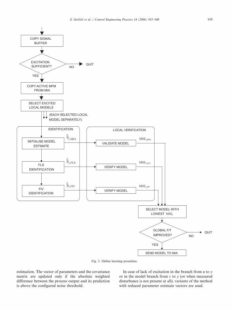
The following procedure, illustrated in Fig. 3, isexecuted when the OLA is invoked.

2.2.1. Copy signal buffer

The buffer of the real-time signals is maintained bythe SPA. When the OLA is invoked, the relevant sectionof the buffer is copied for further processing.

2.2.2. Excitation check

A quick excitation check is performed at the start, sothat processing of the signals is performed only when

they contain excitation. If the standard deviations of thesignals r(k), y(k), u(k), and v(k) in the active buffer arebelow their thresholds, the execution is cancelled.

2.2.3. Copy active MFM from MIA

The online learning procedure always compares thenewly identified local models with the previous set ofparameters. Therefore, the active MFM is copied fromthe MIA where it is stored. A default set of modelparameters is used for the local models that have not yetbeen identified (see Section 2.3).

2.2.4. Select local models

A local model is selected if the sum of its membershipfunctions bj(k) over the active buffer normalised bythe active buffer length exceeds a given threshold.Only the selected local models are included in furtherprocessing.

2.2.5. Identification

The local model parameters are identified using thefuzzy instrumental variables (FIV) identification methoddeveloped by Blazic et al. (2003). It is an extension of thelinear instrumental variables identification procedure(Ljung, 1987) for the specified MFM, based on the locallearning approach (Murray-Smith & Johansen, 1997).The local learning approach is based on the assumptionthat the parameters of all local models will not beestimated in a single regression operation. Compared tothe global approach it is less prone to the problems ofill-conditioning and local minima.

This method is well suited to the needs of industrialoperation (intuitiveness, gradual building of the non-linear model, modest computational demands). Itenables inventory of the local models that are notestimated properly due to insufficient excitation. It isefficient and reliable in early configuration stages, whenall local models have not been estimated yet. On theother hand, the convergence in the vicinity of theoptimum is slow. Therefore, it is likely to yield a worsemodel fit than methods employing nonlinear optimisa-tion. The following briefly describes the procedure.

Model identification is performed for each selectedlocal model (denoted by the index j) separately. Theinitial estimated parameter vector hj;MIA is copied fromthe active MFM, and the covariance matrix Pj,MIA isinitialised to 105 I (identity matrix). The FLS (fuzzyleast-squares) estimates, hj;FLS and Pj,FLS, are obtainedusing weighted least-squares identification, with bj(k)used for weighting. The calculation is performedrecursively to avoid matrix inversion. The FIV (fuzzyinstrumental variables) estimates, hj;FIV and Pj,FIV, arecalculated using weighted instrumental variables identi-fication.

In order to prevent result degradation by noise, adead zone is used in each step of FIV and FLS recursive

ARTICLE IN PRESS

Fig. 3. Online learning procedure.

S. Gerksic et al. / Control Engineering Practice 14 (2006) 935–948 939

estimation. The vector of parameters and the covariancematrix are updated only if the absolute weighteddifference between the process output and its predictionis above the configured noise threshold.

In case of lack of excitation in the branch from u to y

or in the model branch from v to y (or when measureddisturbance is not present at all), variants of the methodwith reduced parameter estimate vectors are used.

ARTICLE IN PRESSS. Gerksic et al. / Control Engineering Practice 14 (2006) 935–948940

2.2.6. Verification/validation

This step is performed by comparing the simulationoutput of a selected local model with the actual processoutput in the proximity of the local model position. Thenormalised sum of mean square errors (MSEj) iscalculated. The proximity is defined by the membershipfunctions bj. For each of the selected local models, thisstep is carried out with three sets of model parameters:hj;MIA; hj;FLS; and hj;FIV: The set with the lowest MSEj isselected.

Then, global verification is performed by comparingthe simulation output of the fuzzy model including theselected set with the actual process output. The normal-ised sum of mean square errors (MSEG) is calculated. Ifthe global verification result is improved compared tothe initial fuzzy model, the selected set is sent to theMIA as the result of online learning, otherwise theoriginal set hj;MIA remains in use.

For each processed local model, the MIA receives theMSEj, which serves as a confidence index, and a flagindicating whether the model is new or not.

2.2.7. Model structure estimation

Two model structure estimation units are alsoincluded in the OLA. The dead-time unit (DTU)estimates the process time delay. The membershipfunction unit (MFU) suggests whether a new localmodel should be inserted. It estimates an additionallocal model in the middle of the interval between the twoneighbouring local models that are the most excited. Themodel is submitted to the MIA if the global validationof the resulting fuzzy model is sufficiently improved,compared to the original fuzzy model.

2.3. Model Information Agent (MIA)

The task of the MIA is to maintain the active MFMand its status information.

Its primary activity is processing the online learningresults. When a new local model is received from theOLA, it is accepted if it passes the stability test and itsconfidence index is sufficient. If it is accepted, a ‘‘readyfor tuning’’ flag is set for the CAA. Another flagindicates whether the local model has been tuned sincestart-up or not. If the model confidence index is verylow, the automatic mode may be disabled.

The MIA contains a mechanism for inserting addi-tional local models into the MFM. This may occureither by request or automatically, using the MFU ofthe OLA. The MIA may also store the active MFM to alocal database or recall a previously stored one, which isuseful for changing of modes.

At initial configuration, the MIA is filled with defaultlocal models based on the initial estimation of theprocess dynamics. They are not exact but may providereliable (although sluggish) control performance, similar

to the Safe mode. Using online learning throughexperiments or normal operating records (when theconditions are appropriate for closed-loop identifica-tion), an accurate model of the plant is estimatedgradually by receiving identified local models fromthe OLA.

2.4. Control Algorithm Agent (CAA)

The CAA comprises an industrial nonlinear controlalgorithm and a procedure for automatic tuning of itsparameters from the MFM. Several different CAAs maybe used in the controller and may be interchanged in theinitial configuration phase.

The following modes of operation are supported:

�

Manual mode: open-loop operation (actuator con-straints are enforced). � Safe mode: a fixed PI controller with conservatively

tuned parameters.

� Auto mode (or several auto modes with different

tuning parameters): a nonlinear controller.

The CAAs share a common interface of interactionwith the OS and a common modular internal structure,consisting of three layers:

1.

The control layer offers the functionality of a locallinear controller (or several local linear controllerssimultaneously), including everything required forindustrial control, such as handling of constraintswith anti-windup protection, bump-less mode switch-ing, etc.

2.

The scheduling layer performs real-time switching orscheduling (blending) of tuned local linear control-lers, so that in conjunction with the control layer afixed-parameter nonlinear controller is realised.

3.

The tuning layer executes the automatic tuningprocedure of the controller parameters from theMFM when the MIA reports that a new local modelis generated if auto-tuning is enabled. The parametersof the control layer and the scheduling layer arereplaced in such a manner that real-time control isnot disturbed.

Three CAAs have been developed and each has beenproved effective in specific applications: the Fuzzyparameter-scheduling controller (FPSC), the dead-timecompensation controller (DTCC), and the rule-basedneural controller (RBNC). In this paper, only theconcept of the FPSC is described briefly in the followingsubsection.

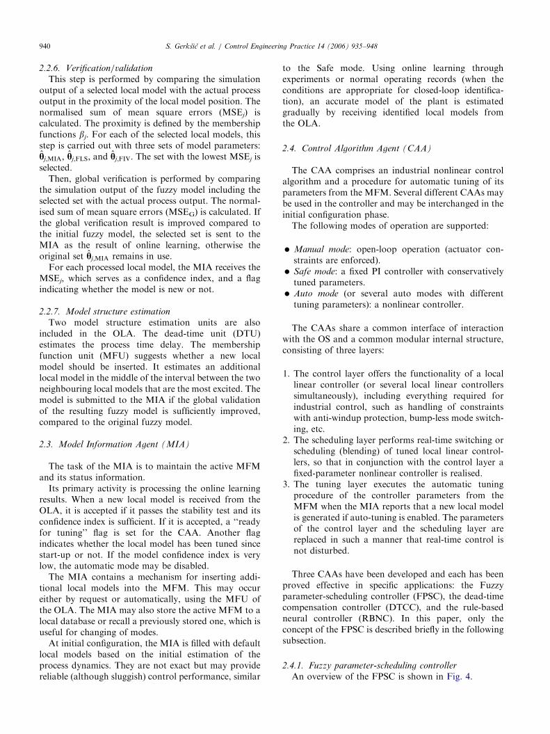
2.4.1. Fuzzy parameter-scheduling controller

An overview of the FPSC is shown in Fig. 4.

ARTICLE IN PRESS

Fig. 4. FPSC overview.

S. Gerksic et al. / Control Engineering Practice 14 (2006) 935–948 941

The control layer of the FPSC includes a single PIDcontroller in the form suitable for controller blendingusing velocity-based linearisation. It is equipped withanti-windup protection and bump-less transfer.

The scheduling layer of the FPSC performs fuzzyblending of the controller parameters (in the case of Ti,its inverse value) according to the scheduling variables(k) and the membership functions bj(k) of the localmodels. The instrument of velocity-based linearisationenables the dynamics of the blended global controller tobe a linear combination of the local controller dynamicsin the entire operating region, not just around equili-brium operating points. This provides the potential toimprove performance with few local models and moretransparent behaviour in off-equilibrium operatingpoints (Leith & Leithead, 1998; Kocijan, Zunic,Strmcnik, & Vrancic, 2002).

The tuning layer of the FPSC is based on themagnitude optimum (MO) criterion implemented usingthe multiple integration (MI) method (Vrancic,Strmcnik, & Juricic, 2001). The MO criterion makesthe magnitude (amplitude) of the system closed-loop set-point response as flat and close to unity as possible for alarge bandwidth (Whiteley, 1946). This results in a

relatively fast and nonoscillatory response of the closed-loop system. The expressions for calculating the PIDcontroller parameters using the MO criterion are quitecomplex. However, the MI method significantly simpli-fies the equations and enables the calculation of the PIDcontroller parameters directly from the process open-loop time response.

The auto-tuning procedure starts by receiving adiscrete-time local model from the MIA. The model isconverted into a continuous-time local model. Then, theso-called areas are calculated from the model using theMI method. Finally, the PI and PID controllerparameters are calculated from the areas. Thanks tothe transparent concept of the FPSC, an experiencedengineer may choose to configure the control algorithmmanually by specifying the local PID controller posi-tions and parameters, without using the model-basedtuning procedure.

2.5. Control performance monitor (CPM)

The CPM scans the buffer of recent real-time signalsfor recognisable events. When events are detected, itestimates the features of closed-loop control response

ARTICLE IN PRESSS. Gerksic et al. / Control Engineering Practice 14 (2006) 935–948942

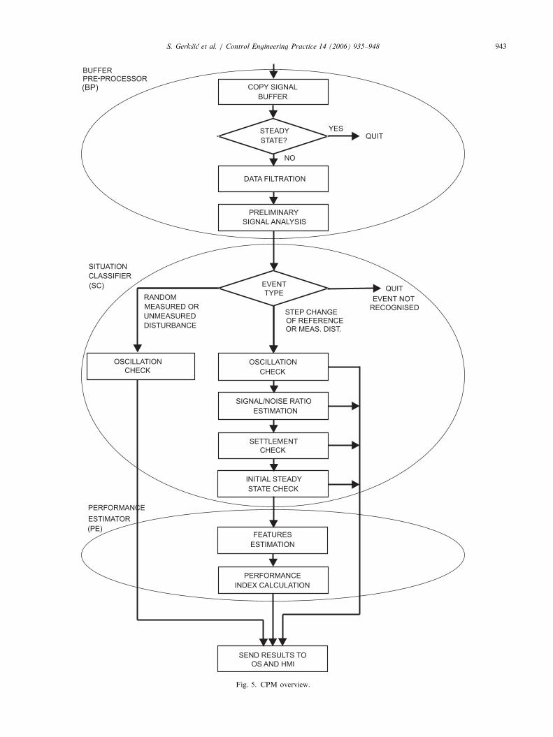
and an overall performance index. Like the OLA, it isinvoked autonomously or upon demand from the OSand runs as a low-priority task. It consists of threemodules: the buffer pre-processor (BP), the situationclassifier (SC), and the performance estimator (PE), asshown in Fig. 5.

When the CPM is invoked, the BP copies the relevantsection of the buffer of the real-time signals, which ismaintained by the SPA. It checks if the process is in asteady-state; if so, it terminates processing. Otherwise, itfilters the signals y and v and performs a low-levelanalysis. The SC scans the pre-processed buffer for thelast recognisable event that may be evaluated, or isotherwise important, e.g., a step change of the referencesignal, a step change of the measured disturbance signal,an occurrence of an unmeasured disturbance, or thepresence of oscillation. If an event that may be evaluatedis detected and the conditions for feature estimation arefulfilled (there is no excessive oscillation, the signal-to-noise ratio is sufficient, the process response has settledafter the event and there was a period of steady-statebefore the event), the corresponding buffer interval issent to the PE, otherwise the execution is terminated.

The PE may extract the following features of detectedevents: overshoot, settling time, rise time, oscillationdecay rate, and tracking error measure or regulationerror measure. Using a fuzzy evaluation procedure, anoverall performance index (PI) is also calculated fromthe features.

The CPM results are sent to the human–machineinterface. If poor performance is detected, the CPMtriggers an automatic switchover to the Safe mode.Other automatic actions include, for example, blockingthe OLA if oscillation is detected. Modifications of theCAA parameters based on CPM results are notgenerally performed because such actions are highlyprocess-specific, but they may be implemented in specificapplications.

2.6. Operation supervisor (OS)

The OS coordinates the control, modelling, andtuning activities of the agents and user interactionthrough the hierarchical set of dialogue windows of thehuman-machine interface (HMI). The OS and the HMIinclude the functionality required for automatic user-friendly experimentation, which is usually required forcontroller tuning.

The controller commissioning procedure comprisesthe phases of basic settings, approximate estimation ofthe process dynamics for safe controller tuning, non-linear modelling and tuning of the scheduling controller,and configuring the regime for regular operation.

The OS supports the control engineer by automaticexecution of experiments for identification of localmodels. These experiments consist of a series of step

changes about the operating point of the model in eitheropen or closed loop. In addition, the OS coordinates theOLA, the MIA and the CAA to automatically processthe signals, build the model and tune the localcontrollers. This is the fastest and most reliable way ofcontroller tuning when experimentation with the plant isallowed. Automatic conducting of experiments forclosed-loop performance testing using the CPM is alsosupported.

Alternatively, scheduling of experiments may not berequired if experimentation is not allowed. In this case,the controller is initialised in the safe mode, andprocessing of the signals for modelling and tuning istriggered by the OLA autonomously. However, it isrequired that sufficient excitation over the wholeoperating region is available during regular operation.The modelling progress is indicated by the statusflags of the local models in the MIA. The flags showwhich models have been tuned and their confidenceindices.

While initiative and suggestions of the agents arehelpful during system configuration, this may not bedesired during regular operation. Therefore, at the endof the commissioning procedure, the system may bereconfigured to simplify the operation as much aspossible.

A range of operating regimes can be configured byenabling or disabling the agents and changing theirconfiguration parameters. This results in a flexiblecontrol system that covers the requirements of a widerange of applications and may help diagnose problems.Thus, although designed for control of nonlinearprocesses, the ASPECT controller may also be usedfor adaptive control using a single linear model or as atool for PID controller tuning. Some specific operatingregime options are listed below:

�

The OLA and/or the CPM may be invoked autono-mously (during regular operation) or upon OSdemand (following scheduled experiments), or both. � The OLA may estimate the process dead-time

continuously or not.

� The OLA may attempt to insert additional local

models when appropriate, or estimate the localmodels at the fixed pre-selected positions only.

� Controller retuning may be triggered automatically

immediately after each change of the model in MIA(‘‘adaptive’’ operation), or following an engineer’sconfirmation (‘‘self-tuning’’ operation).

� Online learning may also be used for monitoring of

the process dynamics without the intention ofcontroller tuning, either by adaptation of the modelor by cross-validation of a fixed model.

At start up, the system is initialised from a config-uration file, which may put it into any phase of the

ARTICLE IN PRESS

Fig. 5. CPM overview.

S. Gerksic et al. / Control Engineering Practice 14 (2006) 935–948 943

ARTICLE IN PRESSS. Gerksic et al. / Control Engineering Practice 14 (2006) 935–948944

configuration procedure. Afterwards, the configurationprocedure may be continued or repeated using the HMIdialogue windows.

3. Configuration tool

The CT is used on a PC, connected to the PLCrunning the RTM. The CT contains a configuration‘‘wizard’’ that guides the engineer through the typicalscheduling controller commissioning procedure. It isintended for less experienced users. Experienced en-gineers may find it more efficient to perform configura-tion only using the RTM, where other sequences of thetasks are possible.

The procedure is decomposed into small steps (25dialogue windows). In each step, instructions aredisplayed and default values are suggested by usingrules of thumb, based on the information alreadyavailable. Inconsistency warnings may be displayed.

The main phases of the configuration procedure are:

�

Basic settings: selection of the control signals, thesignal limits, the sampling time, the control algo-rithm, the scheduling variable, the model order. � Safe mode configuration: estimation of the process

dynamics (experimentation and identification usingthe RTM may be used), self-tuning of the ‘‘safe’’controller parameters (using the RTM), optionalperformance verification.

� Fuzzy model initialisation: initialisation of the model

positions, initialisation of the local model parameters,display of the local model parameters and stepresponses.

� CAA settings: initialisation of the default values,

advanced auto-tuning parameters.

� OLA settings: initialisation of the default values,

advanced OLA settings.

� CPM settings: initialisation of the default values,

advanced CPM settings.

� Experiment settings: initialisation of the default

values, advanced automatic experimentation settings.

� Local controller tuning: sequence of automatic

(open- or closed-loop) experimentation, online learn-ing and tuning using the RTM around each localmodel position.

�

Fig. 6. Apparatus for testing of hydraulic valve (simplified).

Performance verification: sequence of automaticexperimentation and performance evaluation usingthe RTM around each local model position.

The CT relies on the functionality of the RTMwherever possible. However, the PC developmentenvironment is more convenient for graphical userinterface design and enables better visualisation ofresults, compared to typical PLC systems.

4. Field test

The ASPECT controller has been tested in severalpilot applications, for example on a pH control bench-mark (Blazic et al., 2003) and a gas–liquid separator(Kocijan et al., 2003). This section presents a pilotapplication on an apparatus for testing hydraulic valves,located in a hydraulic equipment production plant. Asimplified scheme of the apparatus is shown in Fig. 6. Itcomprises a boiler with local temperature control, threepumps, a pressure sensor, a valve test stand with apressure difference sensor, three flow meters that may beconnected alternately for different measurement ranges,and an expansion vessel. The pumps P1, P2 and P3 areconnected in parallel and may be activated in differentcombinations so that different flow ranges may beachieved. They are equipped with frequency converters;when switched on, all of them receive the same controlsignal u.

The apparatus is used to test the valves in a range ofcontrolled operating conditions. The most importantcontrol task is to control the pressure difference on thetested valve (pv) by adjusting the control signal u that isconnected to the active pumps. The process is nonlinearand time-varying due to the following:

(a)

the steady-state relation between the pressuredifference on the valve pv and the mass flow throughthe valve Qm (related to the pump rotation speed o)is quadratic,

(b)

the openness of the valve Sv can be changed during atest, while the signal Sv is generally not available(manual valves), and

(c)

different pumps (or combinations of pumps) can beused, according to the size of the valve.

These factors severely affect the process dynamics,which results in the unsatisfactory performance of apreviously existing control system based on a fixed PIcontroller.

ARTICLE IN PRESSS. Gerksic et al. / Control Engineering Practice 14 (2006) 935–948 945

Scheduling variable selection is a crucial step whenapplying a parameter-scheduling controller. While thenonlinearity (a) alone may be easily solved usingscheduling from pv, the condition (b) makes the problemconsiderably more difficult. Process modelling was usedto find a suitable scheduling variable1.

4.1. Process modelling

A simplified model of the process is a hydraulic loopthat comprises a pump (subscript p) as a flow generator,two resistive components, the examined valve (subscriptv) and the resistance of the pipeline (subscript l). Theinertia of the liquid in the pipeline acts as an inductivecomponent. Using Newton’s second law, this is de-scribed as

pp � pv � pl

� �S ¼ m

dv

dt¼

m

rS

dQm

dt, (5)

where pp, pv, and pl are the pressure differences at thepump, the valve and the pipeline, S is the pipeline cross-section, and m, v, r, and Qm are the mass, velocity,density, and mass flow of the liquid. Applying locallinearisation about the operating point ðpp; pv; pl ;QmÞ;differentiation of Eq. (5) yields

Dpp � Dpv � Dpl ¼m

rS2

dDQm

dt. (6)

Assuming the valve and pipeline resistance characteristicequations

Qm ¼ kvSvffiffiffiffiffipv

p, (7)

Qm ¼ klSffiffiffiffipl

p, (8)

where kv and kl are the valve and pipeline resis-tance coefficients, Dpv and Dpl are calculated usingpartial derivation about the operating point (Karba,1999)

Dpv ¼2pv

Qm

DQm þ�2pv

Sv

DSv ¼ RvDQm � bvj jDSv, (9)

Dpl ¼2pl

Qm

DQm ¼ RlDQm, (10)

where the coefficients Rv, Rl and bv are introduced forshorter notation (bv is negative). Similarly, Rp and bp areintroduced to describe the pump and may be determinedfrom pump characteristics

Dpp ¼ � Rp

�� ��DQm þ bpDo. (11)

1The ASPECT controller is designed to be tuned empirically through

experimentation, and process modelling is not generally required.

Inserting Eqs. (9)–(11) into Eq. (6), the dynamicresponse of the hydraulic loop is described by

1

Rp

�� ��þ Rv þ Rl

m

rS2

dDQm

dtþ DQm

¼1

Rp

�� ��þ Rv þ Rl

bpDoþ bvj jDSv

� �ð12Þ

or, replacing the internal variable DQm by the processoutput Dpv using Eq. (9), by

1

Rp

�� ��þ Rv þ Rl

m

rS2

dDpv

dtþ Dpv

¼Rv

Rp

�� ��þ Rv þ Rl

bpDo

� bvj jRp

�� ��þ Rl

Rp

�� ��þ Rv þ Rl

�1

Rp

�� ��þ Rl

m

rS2

dDSv

dtþ DSv

!. ð13Þ

Additionally, the relation between the pump controlsignal u and speed o, describing the dynamics of thepump motor with the frequency converter, must begiven. It may be described by a first order lag

Tp1dDodtþ Do ¼ bp1Du, (14)

where bp1 is the gain coefficient and Tp1 the timeconstant. Therefore, second order dynamics of thecontrolled process is assumed.

Observing Eq. (13), Rv ¼ 2pv=Qm is a good schedulingvariable candidate because it represents a property ofthe examined valve at the current operating point thataffects both the gain and the time constant of thecontrolled process. It may be calculated directly fromthe available process measurements. To improve thestability of the quotient computation at low measure-ment values, for the actual scheduling variable in theimplemented control system the Qm measurement wasreplaced by the control signal u that was filteredaccording to the model in Eq. (14); after division, safetyconstraints were applied.

4.2. Experimental Trial

Once the scheduling variable is selected, the commis-sioning of the controller is an empirical procedure,supported by the automatic experimentation function-ality of the OS. Firstly, a conventional PI controller istuned for the Safe mode so that it maintains stablecontrol over the operating region. Then, the localmodel/controller positions are selected. In this applica-tion, a default equidistant distribution of six positionsover the operating range of s is used.

ARTICLE IN PRESSS. Gerksic et al. / Control Engineering Practice 14 (2006) 935–948946

Because experimentation with the process is allowed,the typical procedure involving experiments aroundeach local model position is used. In practice, this is thesimplest way to ensure proper excitation of the signals.Using the Safe mode, the process is consecutivelybrought to each of the positions, where auto-tuningexperiments are activated by the push of a button. TheOS conducts a mode switch (open-loop experiments arepreferred), injects the excitation signal containing four

Table 1

Scheduling variable positions, discrete-time local model parameters, derived

Local model positions Local model parameters

OLA model parameters (Tsamp ¼ 0.5 s)

s ¼ ayu

du b1 b2 a1 a2 r

0.10 1 0.002 0.009 �1.212 0.256 �0.0

0.26 1 0.003 0.014 �1.369 0.410 �0.0

0.42 1 0.004 0.017 �1.392 0.432 �0.0

0.58 1 0.003 0.022 �1.401 0.442 �0.0

0.74 1 0.001 0.026 �1.471 0.508 �0.0

0.90 1 -0.001 0.044 �1.397 0.440 �0.0

aT90% is the rise time from 0 to 90% of open-loop step response in s, T

equivalent model in s, and Kol is the open-loop model gain. a ¼ 1.89 is a sc

Fig. 7. Control of pressure difference pv using the PI controller.

step changes, invokes the identification-tuning proce-dure at the end of the experiment and restores theoriginal mode. For the first two local models, theexcitation signal amplitude is 4%. Due to lower processgain it is increased to 8% for other local models,to improve the signal-to-noise ratio. An overviewof the MIA status shows that all local models havebeen identified successfully. The Auto mode is config-ured after the engineer confirms the new controller

local model parameters, and local controller parameters

Local controller parameters

Derived parametersa

Kol T90% T1 T2 Kp Ti

02 0.25 20.0 8.01 0.38 5.78 8.03

02 0.41 16.5 6.55 0.61 2.58 6.56

05 0.52 16.5 6.41 0.66 1.95 6.29

05 0.61 15.5 6.09 0.68 1.54 6.12

08 0.73 15.0 5.77 0.85 1.14 5.92

19 1.00 15.0 5.80 0.69 0.86 5.97

1 and T2 are the denominator time constants of the continuous-time

aling factor.

SP,

pv

(%)

u, s

(%

)

Fig. 8. Control of pressure difference pv using the FPSC algorithm.

ARTICLE IN PRESSS. Gerksic et al. / Control Engineering Practice 14 (2006) 935–948 947

parameters. Table 1 displays the results of this experi-mental tuning procedure on the process.

The open-loop gain of the local models obviouslyrises with s (and Rv) in full accordance with the model inEq. (13), which results in decreasing of Kp. The changesof the identified time constant T2 are less obvious and donot appear to be consistent with the dependence of thetime constant in Eq. (13) on Rv, however Rl and |Rp|vary as well but are not measurable. The variation of Ti

mostly results from the changes in T1, which isassociated wtih the pump dynamics Tf1. There isconsiderable but acceptable difference in Kp betweenthe first two local controllers. The differences betweenthe local controller parameters in the higher range of s

are small; fewer local controllers could be used in thatregion.

The control performance is shown for the PIcontroller, realised using the safe mode of the ASPECTcontroller, and the FPSC controller. Fig. 7 shows themeasured process response to a sequence of step changesof the set-point signal over the whole operating rangewhen using the PI controller. The pressure difference atthe valve pv and the set-point (SP) are shown above, andthe pump control signal u below. The parameters of thePI controller were determined so that optimal response

Fig. 9. Valve pressure control schem

was achieved at lower values of pv. As the pressureincreased, the response became oscillatory.

Fig. 8 shows the response when using the FPSCcontrol algorithm. In addition to the signals shown inFig. 7, the scheduling variable s is also shown in thebottom graph of Fig. 8. In comparison to the PIcontroller of Fig. 7, this response is optimal over theentire operating region.

4.3. Test platform

Despite the careful selection and modification of thealgorithms to reduce computational demand, the OLAand CPM modules are not suitable for implementationin typical PLCs. A DSP or open controller add-onmodule tends to be a more cost-effective solution thanan upper-market PLC. The test platform running theRTM of the ASPECT controller in this pilot applicationconsisted of a Mitsubishi A1S series PLC with an INEAIDR SPAC20 coprocessor, based on the Texas Instru-ments DSP TMS320C32 at 40MHz with 2MB of RAM,and a Mitsubishi MAC E700 HMI unit.

The RTM is an extension for INEA IDR BLOK, agraphical development tool for closed-loop controlapplications in the process industry using Mitsubishi

e designed using IDR BLOK.

ARTICLE IN PRESSS. Gerksic et al. / Control Engineering Practice 14 (2006) 935–948948

Electric MELSEC AnSH PLC controllers (INEA d.o.o.,2001). The FPSC algorithm is included as an additionalcontroller block ‘‘PID/FPSC’’. Other RTM componentsare implemented as separate PLC tasks, coded in C anddownloaded to the PLC in compiled form. They aresupervised using the HMI unit through a hierarchical setof menus (such as: Operator display, Trends display,Settings overview, Experiment settings, Online learningsettings, Model parameters, Model status, FPSC set-tings, FPSC parameters, etc.).

Fig. 9 displays the valve pressure control schemedesigned in the IDR BLOK environment. Unfortu-nately, the current version does not yet indicate theassociation of the PID/FPSC controller block with thesupervisory tasks of the RTM.

5. Conclusion

An advanced self-tuning nonlinear controller has beensuccessfully implemented on an industrial PLC plat-form. Several pilot applications, including the onepresented in this paper, have also been successfullycompleted. Compared to the industry standard PIcontroller, an expected considerable improvement inthe control performance was achieved using the FPSCcontrol algorithm. Moreover, this performance waseasily achieved in practice with self-tuning using theonline learning procedure, by performing a sequence ofshort experiments around a few operating points. Themodular multi-agent structure contributes to remark-able flexibility of the control system, so that it is easilyreconfigured for various requirements. The work iscurrently directed towards further improvements in thesimplicity of use and ease of application to newprocesses. A promising future research direction is theincorporation of the pattern recognition techniquesfrom the CPM in data evaluation in the online learningprocedure, which may result in a positive contributionto the reliability of adaptive control.

Acknowledgment

The authors would like to acknowledge the contribu-tions of all other project team members. The ASPECTproject was financially supported by EC under contractIST-1999-56407. ASPECT r2002 software is the prop-erty of INEA d.o.o., Indelec Europe S.A., and StartEngineering JSCo. Patent pending PCT/SI02/00029.

References

Babuska, R., Oosterhoff, J., Oudshoorn, A., & Bruijn, P. M. (2002).

Fuzzy self-tuning PI control of pH in fermentation. Engineering

Applications of Artificial Intelligence, 15, 3–15.

Bequette, B. W. (1991). Non-linear control of chemical processes: A

review. Industrial & Engineering Chemistry Research, 30,

1391–1413.

Blazic, S., Skrjanc, I., Gerksic, S., Dolanc, G., Strmcnik, S., Hadjiski,

M. B., & Stathaki, A. (2003). On-line Fuzzy Identification for

Advanced Intelligent Controller. Proceedings of the IEEE interna-

tional conference on industrial technology ICIT 2003. Maribor,

Slovenia, (pp. 912–916).

Dougherty, D., & Cooper, D. J. (2003). A practical multiple model

adaptive strategy for multivariable model predictive control.

Control Engineering Practice, 11, 649–664.

Gundala, R., Hoo, K. A., & Piovoso, M. J. (2000). Multiple Model

Adaptive Control Design for a Multiple-Input Multiple-Output

Chemical Reactor. Industrial & Engineering Chemistry Research,

39, 1554–1564.

Hagglund, T., & Astrom, K. J. (2000). Supervision of adaptive control

algorithms. Automatica, 36, 1171–1180.

Henson, M. A., & Seborg, D. E. (1994). Adaptive non-linear control of

a pH neutralisation process. IEEE Transactions on Control Systems

Technology, 2, 169–182.

Henson, M. A., & Seborg, D. E. (1997). Non-linear process control.

Upper Saddle River NJ: Prentice-Hall PTR.

INEA d.o.o. (2001). IDR BLOK Process control tools for Mitsubishi

electric PLC’s, user’s manual, Ver. 4.20. Ljubljana: INEA d.o.o.;

http://www.inea.si/index.php?kategorija=158.

Kocijan, J., Zunic, G., Strmcnik, S., & Vrancic, D. (2002). Fuzzy

gain-scheduling control of a gas+liquid separation plant imple-

mented on a PLC. International Journal of Control, 75(14),

1082–1091.

Kocijan, J., Vrancic, D., Dolanc, G., Gerksic, S. Strmcnik, S., Skrjanc,

I., Blazic, S., Bozicek, M., Marinsek, Z., Hadjinski, M. B.,

Boshnakov, K., Stathaki, A., & King, R. (2003). Auto-tuning

non-linear controller for industrial use. Proceedings of the IEEE

international conference on industrial technology ICIT 2003.

Maribor, Slovenia, (pp. 906-910).

Karba, R. (1999). Modeliranje procesov ¼ process modelling (in

Slovenian). Ljubljana: Faculty of Electrical Engineering.

Leith, D. J., & Leithead, W. E. (1998). Appropriate realisation of

MIMO gain-scheduled controllers. International Journal of Con-

trol, 70(1), 13–50.

Ljung, L. (1987). System Identification. Englewood Cliffs, NJ:

Prentice-Hall.

Murray-Smith, R., & Johansen, T. A. (Ed.) (1997). Multiple model

approaches to modelling and control. London, Bristol: Taylor &

Francis.

Seborg, D. E. (1999). A perspective on advanced strategies for process

control (revisited). In P. M. Frank (Ed.), Advances in control,

highlights of ECC’99, (pp. 103–134). London: Springer.

Stephanopoulus, G., Henning, G., & Leone, H. (1990). Model LA—a

modelling language for process engineering, II. Multifaceted

modelling of processing systems. Computers & Chemical Engineer-

ing, 14, 847–869.

Takatsu, H., Itoh, T., & Araki, M. (1998). Future needs for the control

theory in industries—report and topics of the control technology

survey in Japanese industry. Journal of Process Control, 8(5-6),

369–374.

Tan, S., Hang, C.-C., & Chai, J.-S. (1997). Gain scheduling: From

conventional to neuro-fuzzy. Automatica, 33(3), 411–419.

Vrancic, D., Strmcnik, S., & Juricic, �. (2001). A magnitude optimum

multiple integration tuning method for filtered PID controller.

Automatica, 37, 1473–1479.

Whiteley, A. L. (1946). Theory of servo systems with particular

reference to stabilization. The Journal of IEE, Part II, 93(34),

353–372.

Wooldridge, M., & Jennings, N. R. (1995). Intelligent agents theory

and practice. Knowledge Engineering Review, 10(2), 115–152.