Advanced Computer Architecture- 06CS81- Unit...
35
Advanced Computer Architecture- 06CS81- Unit 8 Loop Level Parallelism- Detection and Enhancement Static Exploitation of ILP •Use compiler support for increasing parallelism –Supported by hardware •Techniques for eliminating some types of dependences –Applied at compile time (no run time support) •Finding parallelism •Reducing control and data dependencies •Using speculation Unrolling Loops – High-level –for (i=1000; i>0; i=i-1) x[i] = x[i] + s; –C equivalent of unrolling to block four iterations into one: –for (i=250; i>0; i=i-1) { x[4*i] = x[4*i] + s; x[4*i-1] = x[4*i-1] + s; x[4*i-2] = x[4*i-2] + s; x[4*i-3] = x[4*i-3] + s; } Enhancing Loop-Level Parallelism •Consider the previous running example: –for (i=1000; i>0; i=i-1) x[i] = x[i] + s; –there is no loop-carried dependence – where data used in a later iteration depends on data produced in an earlier one –in other words, all iterations could (conceptually) be executed in parallel •Contrast with the following loop: –for (i=1; i<=100; i=i+1) { A[i+1] = A[i] + C[i]; /* S1 */ B[i+1] = B[i] + A[i+1]; /* S2 */ } –what are the dependences? A Loop with Dependences •For the loop: –for (i=1; i<=100; i=i+1) { A[i+1] = A[i] + C[i]; /* S1 */ B[i+1] = B[i] + A[i+1]; /* S2 */ } –what are the dependences? •There are two different dependences: –loop-carried: (prevents parallel operation of iterations) •S1 computes A[i+1] using value of A[i] computed in previous iteration •S2 computes B[i+1] using value of B[i] computed in previous iteration –not loop-carried: (parallel operation of iterations is ok) •S2 uses the value A[i+1] computed by S1 in the same iteration •The loop-carried dependences in this case force successive iterations of the loop to execute in series. Why? –S1 of iteration i depends on S1 of iteration i-1 which in turn depends on …, etc.
Transcript of Advanced Computer Architecture- 06CS81- Unit...

Advanced Computer Architecture- 06CS81- Unit 8
Loop Level Parallelism- Detection and Enhancement Static Exploitation of ILP
•Use compiler support for increasing parallelism
–Supported by hardware
•Techniques for eliminating some types of dependences
–Applied at compile time (no run time support)
•Finding parallelism
•Reducing control and data dependencies
•Using speculation
Unrolling Loops – High-level
–for (i=1000; i>0; i=i-1) x[i] = x[i] + s;
–C equivalent of unrolling to block four iterations into one:
–for (i=250; i>0; i=i-1)
{
x[4*i] = x[4*i] + s;
x[4*i-1] = x[4*i-1] + s;
x[4*i-2] = x[4*i-2] + s;
x[4*i-3] = x[4*i-3] + s;
}
Enhancing Loop-Level Parallelism
•Consider the previous running example:
–for (i=1000; i>0; i=i-1) x[i] = x[i] + s;
–there is no loop-carried dependence – where data used in a later iteration depends on
data produced in an earlier one
–in other words, all iterations could (conceptually) be executed in parallel
•Contrast with the following loop:
–for (i=1; i<=100; i=i+1) { A[i+1] = A[i] + C[i]; /* S1 */
B[i+1] = B[i] + A[i+1]; /* S2 */ }
–what are the dependences?
A Loop with Dependences
•For the loop:
–for (i=1; i<=100; i=i+1) { A[i+1] = A[i] + C[i]; /* S1 */
B[i+1] = B[i] + A[i+1]; /* S2 */ }
–what are the dependences?
•There are two different dependences:
–loop-carried: (prevents parallel operation of iterations) •S1 computes A[i+1] using value of A[i] computed in previous iteration
•S2 computes B[i+1] using value of B[i] computed in previous iteration
–not loop-carried: (parallel operation of iterations is ok) •S2 uses the value A[i+1] computed by S1 in the same iteration
•The loop-carried dependences in this case force successive iterations of the loop to
execute in series. Why?
–S1 of iteration i depends on S1 of iteration i-1 which in turn depends on …, etc.

Another Loop with Dependences
•Generally, loop-carried dependences hinder ILP
–if there are no loop-carried dependences all iterations could be executed in parallel
–even if there are loop-carried dependences it may be possible to parallelize the loop – an
analysis of the dependences is required…
•For the loop:
–for (i=1; i<=100; i=i+1) { A[i] = A[i] + B[i]; /* S1 */
B[i+1] = C[i] + D[i]; /* S2 */ }
–what are the dependences? •There is one loop-carried dependence:
–S1 uses the value of B[i] computed in a previous iteration by S2
–but this does not force iterations to execute in series. Why…?
–…because S1 of iteration i depends on S2 of iteration i-1…, and the chain of
dependences stops here!
Parallelizing Loops with Short Chains of Dependences •Parallelize the loop:
–for (i=1; i<=100; i=i+1) { A[i] = A[i] + B[i]; /* S1 */
B[i+1] = C[i] + D[i]; /* S2 */ }
•Parallelized code:
–A[1] = A[1] + B[1];
for (i=1; i<=99; i=i+1)
{ B[i+1] = C[i] + D[i];
A[i+1] = A[i+1] + B[i+1];
}
B[101] = C[100] + D[100];
–the dependence between the two statements in the loop is no longer loop-carried and
iterations of the loop may be executed in parallel
–
Loop-Carried Dependence Detection: affine array index: a x i+b To detect loop-carried dependence in a loop, the Greatest Common Divisor (GCD) test
can be used by the compiler, which is based on the following:
If an array element with index: a x i + b is stored and element: c x i + d of
the same array is loaded later where index runs from m to n, a dependence exists if
the following two conditions hold:
1.There are two iteration indices, j and k , m <= j , k <= n
(within iteration limits)
2.The loop stores into an array element indexed by:
a x j + b
and later loads from the same array the element indexed by:
c x k + d
Thus:
a x j + b = c x k + d

The Greatest Common Divisor (GCD) Test If a loop carried dependence exists, then :
GCD(c, a) must divide (d-b) The GCD test is sufficient to guarantee no loop carried dependence
However there are cases where GCD test succeeds but no dependence exits because GCD
test does not take loop bounds into account
Example:
for (i=1; i<=100; i=i+1) {
x[2*i+3] = x[2*i] * 5.0;
}
a = 2 b = 3 c = 2 d = 0
GCD(a, c) = 2
d - b = -3
2 does not divide -3 � No loop carried dependence possible.
Example- Loop Iterations to be Independent Finding multiple types of dependences
for (i=1; i<=100; i=i+1) {
Y[i] = X[i] / c; /* S1 */
X[i] = X[i] + c; /* S2 */
Z[i] = Y[i] + c; /* S3 */
Y[i] = c - Y[i]; /* S4 */ } Answer The following dependences exist among the four statements:
1. There are true dependences from S1 to S3 and from S1 to S4 because of Y[i]. These
are not loop carried, so they do not prevent the loop from being considered parallel.
These dependences will force S3 and S4 to wait for S1 to complete.
2. There is an antidependence from S1 to S2, based on X[i].
3. There is an antidependence from S3 to S4 for Y[i].
4. There is an output dependence from S1 to S4, based on Y[i].
Eliminating false dependencies
The following version of the loop eliminates these false (or pseudo) dependences.
for (i=1; i<=100; i=i+1 { /* Y renamed to T to remove output dependence */
T[i] = X[i] / c; /* X renamed to X1 to remove antidependence */
X1[i] = X[i] + c; /* Y renamed to T to remove antidependence */
Z[i] = T[i] + c;
Y[i] = c - T[i];
}
Drawback of dependence analysis
•When objects are referenced via pointers rather than array indices (but see discussion
below)
• When array indexing is indirect through another array, which happens with many
representations of sparse arrays
• When a dependence may exist for some value of the inputs, but does not exist in
actuality when the code is run since the inputs never take on those values
• When an optimization depends on knowing more than just the possibility of a
dependence, but needs to know on which write of a variable does a read of that variable
depend
Points-to analysis
Relies on information from three major sources: 1. Type information, which restricts what a pointer can point to.
2. Information derived when an object is allocated or when the address of an object is
taken, which can be used to restrict what a pointer can point to. For example, if p always
points to an object allocated in a given source line and q never points to that object, then
p and q can never point to the same object.
3. Information derived from pointer assignments. For example, if p may be assigned the
value of q, then p may point to anything q points to.
Eliminating dependent
computations copy propagation, used to simplify sequences like the following:
DADDUI R1,R2,#4
DADDUI R1,R1,#4
to
DADDUI R1,R2,#8
Tree height reduction
•they reduce the height of the tree structure representing a computation, making it wider
but shorter.
Recurrence Recurrences are expressions whose value on one iteration is given by a function that
depends onthe previous iterations.
sum = sum + x;
sum = sum + x1 + x2 + x3 + x4 + x5;
If unoptimized requires five dependent operations, but it can be rewritten as
sum = ((sum + x1) + (x2 + x3)) + (x4 + x5);
evaluated in only three dependent operations.
Scheduling and Structuring Code for Parallelism Static Exploitation of ILP
•Use compiler support for increasing parallelism
–Supported by hardware
•Techniques for eliminating some types of dependences
–Applied at compile time (no run time support)
•Finding parallelism
•Reducing control and data dependencies
•Using speculation
Techniques to increase the amount of ILP
•For processor issuing more than one instruction on every clock cycle.
–Loop unrolling,
–software pipelining,
–trace scheduling, and
–superblock scheduling
Software pipelining
•Symbolic loop unrolling
•Benefits of loop unrolling with reduced code size
•Instructions in loop body selected from different loop iterations
•Increase distance between dependent instructions in
Software pipelined loop
Loop: SD F4,16(R1) #store to v[i]
ADDD F4,F0,F2 #add to v[i-1]
LD F0,0(R1) #load v[i-2]
ADDI R1,R1,-8
BNE R1,R2,Loop 5 cycles/iteration (with dynamic scheduling and renaming)
Need startup/cleanup code

Software pipelining
(cont.)
SW pipelining example
Iteration i: L.D F0,0(R1)
ADD.D F4,F0,F2
S.D F4,0(R1) Iteration i+1: L.D F0,0(R1)
ADD.D F4,F0,F2 S.D F4,0(R1)
Iteration i+2: L.D F0,0(R1)
ADD.D F4,F0,F2
S.D F4,0(R1)
SW pipelined loop with startup and cleanup code
#startup, assume i runs from 0 to n ADDI R1,R1-16 #point to v[n-2]
LD F0,16(R1) #load v[n]
ADDD F4,F0,F2 #add v[n]
LD F0,8(R1) #load v[n-1]
#body for (i=2;i<=n-2;i++)
Loop: SD F4,16(R1) #store to v[i]
ADDD F4,F0,F2 #add to v[i-1]
LD F0,0(R1) #load v[i-2]
ADDI R1,R1,-8
BNE R1,R2,Loop
#cleanup
SD F4,8(R1) #store v[1]
ADDD F4,F0,F2 #add v[0]
SD F4,0(R1) #store v[0]
Software pipelining versus unrolling

•Performance effects of SW pipelining vs. unrolling
–Unrolling reduces loop overhead per iteration
–SW pipelining reduces startup-cleanup pipeline overhead
Software pipelining versus unrolling (cont.)
Software pipelining
(cont.)
Advantages
•Less code space than conventional unrolling
•Loop runs at peak speed during steady state
•Overhead only at loop initiation and termination
•Complements unrolling
Disadvantages
•Hard to overlap long latencies
•Unrolling combined with SW pipelining
•Requires advanced compiler transformations
Global Code Scheduling
•Global code scheduling aims to compact a code fragment with internal control structure
into the shortest possible sequence that preserves the data and control dependences.

Global code scheduling
•aims to compact a code fragment with internal control
–structure into the shortest possible sequence
–that preserves the data and control dependences
•Data dependences are overcome by unrolling
•In the case of memory operations, using dependence analysis to determine if two
references refer to the same address.
•Finding the shortest possible sequence of dependent instructions- critical path
•Reduce the effect of control dependences arising from conditional nonloop branches by
moving code.
•Since moving code across branches will often affect the frequency of execution of such
code, effectively using global code motion requires estimates of the relative frequency of
different paths.
•if the frequency information is accurate, is likely to lead to faster code.
Global code scheduling- cont.
•Global code motion is important since many inner loops contain conditional statements.
•Effectively scheduling this code could require that we move the assignments to B and C
to earlier in the execution sequence, before the test of A.
Factors for compiler
•Global code scheduling is an extremely complex problem
–What are the relative execution frequencies
–What is the cost of executing the computation
–How will the movement of B change the execution time
–Is B the best code fragment that can be moved
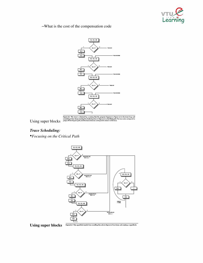
–What is the cost of the compensation code
Using super blocks
Trace Scheduling:
•Focusing on the Critical Path
Using super blocks

Code generation sequence
LD R4,0(R1) ;load A
LD R5,0(R2) ;load B
DADDU R4,R4,R5 ;Add to A
SD R4,0(R1) ;Store A
...
BNEZ R4,elsepart ;Test A
... ;then part
SD ...,0(R2) ;Stores to B
...
J join ;jump over else
elsepart: ... ;else part
X ;code for X
...
join: ... ;after if
SD ...,0(R3) ;store C[i]
Trace Scheduling,
Superblocks and Predicated Instructions
•For processor issuing more than one instruction on every clock cycle.
–Loop unrolling,
–software pipelining,
–trace scheduling, and
–superblock scheduling
Trace Scheduling
•Used when
– Predicated execution is not supported
– Unrolling is insufficient
• Best used
– If profile information clearly favors one path over the other
• Significant overheads are added to the infrequent path
• Two steps :
– Trace Selection
– Trace Compaction
Trace Selection Likely sequence of basic blocks that can be put together
– Sequence is called a trace
• What can you select?

– Loop unrolling generates long traces
– Static branch prediction forces some straight-line code behavior
Trace Selection
(cont.)
Trace Example
If the shaded portion in
previous code was
frequent path and it was
unrolled 4 times : �
• Trace exits are jumps off
the frequent path
• Trace entrances are
returns to the trace
Trace Compaction
•Squeeze these into smaller number of wide instructions
• Move operations as early as it can be in a trace
• Pack the instructions into as few wide instructions as possible
• Simplifies the decisions concerning global code motion
– All branches are viewed as jumps into or out of the trace
• Bookkeeping
– Cost is assumed to be little
• Best used in scientific code with extensive
loops
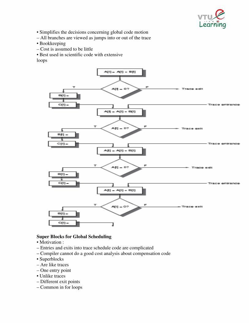
Super Blocks for Global Scheduling • Motivation :
– Entries and exits into trace schedule code are complicated
– Compiler cannot do a good cost analysis about compensation code
• Superblocks
– Are like traces
– One entry point
• Unlike traces
– Different exit points
– Common in for loops
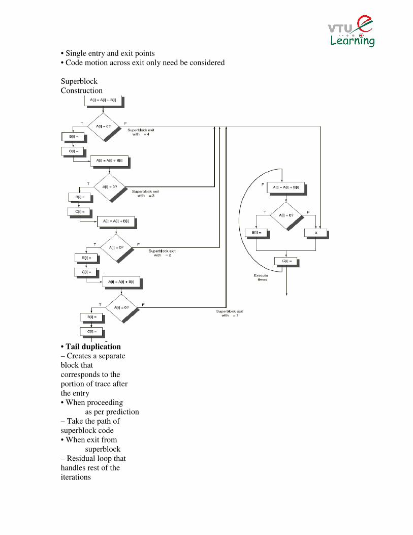
• Single entry and exit points
• Code motion across exit only need be considered
Superblock
Construction
• Tail duplication – Creates a separate
block that
corresponds to the
portion of trace after
the entry
• When proceeding
as per prediction
– Take the path of
superblock code
• When exit from
superblock
– Residual loop that
handles rest of the
iterations

Analysis on Superblocks • Reduces the complexity of bookkeeping and scheduling
– Unlike the trace approach
• Can have larger code size though
• Assessing the cost of duplication
• Compilation process is not simple any more
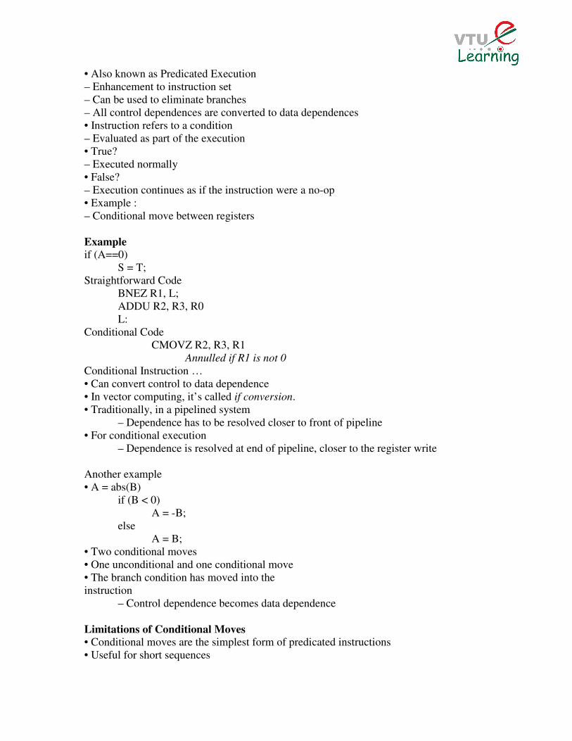
H/W Support : Conditional Execution • Also known as Predicated Execution
– Enhancement to instruction set
– Can be used to eliminate branches
– All control dependences are converted to data dependences
• Instruction refers to a condition
– Evaluated as part of the execution
• True?
– Executed normally
• False?
– Execution continues as if the instruction were a no-op
• Example :
– Conditional move between registers
Example if (A==0)
S = T;
Straightforward Code
BNEZ R1, L;
ADDU R2, R3, R0
L:
Conditional Code
CMOVZ R2, R3, R1
Annulled if R1 is not 0
Conditional Instruction …
• Can convert control to data dependence
• In vector computing, it’s called if conversion.
• Traditionally, in a pipelined system
– Dependence has to be resolved closer to front of pipeline
• For conditional execution
– Dependence is resolved at end of pipeline, closer to the register write
Another example
• A = abs(B)
if (B < 0)
A = -B;
else
A = B;

• Two conditional moves
• One unconditional and one conditional move
• The branch condition has moved into the
instruction
– Control dependence becomes data dependence
Limitations of Conditional Moves • Conditional moves are the simplest form of predicated instructions
• Useful for short sequences
• For large code, this can be inefficient
– Introduces many conditional moves
• Some architectures support full predication
– All instructions, not just moves
• Very useful in global scheduling
– Can handle nonloop branches nicely
– Eg : The whole if portion can be predicated if the frequent path is not taken
Example
• Assume : Two issues, one to ALU and one to memory; or branch by itself
• Wastes a memory operation slot in second cycle
• Can incur a data dependence stall if branch is not taken
– R9 depends on R8
Predicated Execution Assume : LWC is predicated load and loads if third operand is not 0

• One instruction issue slot is eliminated
• On mispredicted branch, predicated instruction will not have any effect
• If sequence following the branch is short, the entire block of the code can be predicated
Some Complications • Exception Behavior
– Must not generate exception if the predicate is false
• If R10 is zero in the previous example
– LW R8, 0(R10) can cause a protection fault
• If condition is satisfied
– A page fault can still occur
• Biggest Issue – Decide when to annul an instruction
– Can be done during issue
• Early in pipeline
• Value of condition must be known early, can induce stalls
– Can be done before commit
• Modern processors do this
• Annulled instructions will use functional resources
• Register forwarding and such can complicate implementation
Limitations of Predicated Instructions • Annulled instructions still take resources
– Fetch and execute atleast
– For longer code sequences, benefits of conditional move vs branch is not clear
• Only useful when predicate can be evaluated early in the instruction stream
• What if there are multiple branches?
– Predicate on two values?
• Higher cycle count or slower clock rate for predicated instructions
– More hardware overhead
• MIPS, Alpha, Pentium etc support partial predication
• IA-64 has full predication
Hardware support for Compiler Speculation H/W Support : Conditional Execution
• Also known as Predicated Execution
– Enhancement to instruction set
– Can be used to eliminate branches
– All control dependences are converted to data dependences
• Instruction refers to a condition
– Evaluated as part of the execution
• True?
– Executed normally
• False?
– Execution continues as if the instruction were a no-op
• Example :
– Conditional move between registers
Example if (A==0)
S = T;
Straightforward Code
BNEZ R1, L;
ADDU R2, R3, R0
L:
Conditional Code
CMOVZ R2, R3, R1
Annulled if R1 is not 0
Conditional Instruction …
• Can convert control to data dependence
• In vector computing, it’s called if conversion.
• Traditionally, in a pipelined system
– Dependence has to be resolved closer to front of pipeline
• For conditional execution
– Dependence is resolved at end of pipeline, closer to the register write
Another example
• A = abs(B)
if (B < 0)
A = -B;
else
A = B;
• Two conditional moves
• One unconditional and one conditional move
• The branch condition has moved into the
instruction
– Control dependence becomes data dependence
Limitations of Conditional Moves • Conditional moves are the simplest form of predicated instructions
• Useful for short sequences
• For large code, this can be inefficient
– Introduces many conditional moves
• Some architectures support full predication
– All instructions, not just moves
• Very useful in global scheduling
– Can handle nonloop branches nicely
– Eg : The whole if portion can be predicated if the frequent path is not taken
Example
• Assume : Two issues, one to ALU and one to memory; or branch by itself
• Wastes a memory operation slot in second cycle
• Can incur a data dependence stall if branch is not taken
– R9 depends on R8
Predicated Execution Assume : LWC is predicated load and loads if third operand is not 0
• One instruction issue slot is eliminated
• On mispredicted branch, predicated instruction will not have any effect
• If sequence following the branch is short, the entire block of the code can be predicated
Predication Some Complications
• Exception Behavior
– Must not generate exception if the predicate is false
• If R10 is zero in the previous example
– LW R8, 0(R10) can cause a protection fault
• If condition is satisfied
– A page fault can still occur
• Biggest Issue – Decide when to annul an instruction
– Can be done during issue
-- Early in pipeline
• Value of condition must be known early, can induce stalls
– Can be done before commit
• Modern processors do this
• Annulled instructions will use functional resources
• Register forwarding and such can complicate implementation
Limitations of Predicated Instructions • Annulled instructions still take resources
– Fetch and execute atleast
– For longer code sequences, benefits of conditional move vs branch is not clear
• Only useful when predicate can be evaluated early in the instruction stream
• What if there are multiple branches?
– Predicate on two values?
• Higher cycle count or slower clock rate for predicated instructions
– More hardware overhead

• MIPS, Alpha, Pentium etc support partial predication
• IA-64 has full predication
Preserve control and data flow, precise interrupts in Predication
•Speculative predicated instructions may not throw illegal exceptions
–LWC may not throw exception if R10 == 0
–LWC may throw recoverable page fault if R10 6= 0
•Instruction conversion to nop
–Early condition detection may not be possible due to data dependence
–Late condition detection incurs stalls and consumes pipeline resources needlessly
•Instructions may be dependent on multiple branches
•Compiler able to find instruction slots and reorder
Hardware support for speculation Alternatives for handling speculative exceptions
•Hardware and OS ignore exceptions from speculative instructions
•Mark speculative instructions and check for exceptions
–Additional instructions to check for exceptions and recover
•Registers marked with poison bits to catch exceptions upon read
•Hardware buffers instruction results until instruction is no longer speculative
Exception classes
•Recoverable: exception from speculative instruction may harm performance, but not
preciseness
•Unrecoverable: exception from speculative instruction compromises preciseness
Solution I: Ignore exceptions
HW/SW solution
•Instruction causing exception returns undefined value
•Value not used if instruction is speculative
•Incorrect result if instruction is non-speculative
–Compiler generates code to throw regular exception
•Rename registers receiving speculative results
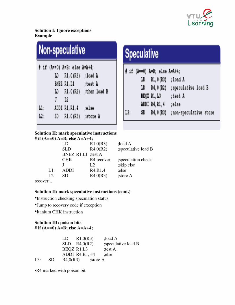
Solution I: Ignore exceptions
Example
Solution II: mark speculative instructions
# if (A==0) A=B; else A=A+4; LD R1,0(R3) ;load A
SLD R4,0(R2) ;speculative load B
BNEZ R1,L1 ;test A
CHK R4,recover ;speculation check
J L2 ;skip else
L1: ADDI R4,R1,4 ;else
L2: SD R4,0(R3) ;store A
recover:..
Solution II: mark speculative instructions (cont.)
•Instruction checking speculation status
•Jump to recovery code if exception
•Itanium CHK instruction
Solution III: poison bits
# if (A==0) A=B; else A=A+4;
LD R1,0(R3) ;load A
SLD R4,0(R2) ;speculative load B
BEQZ R1,L3 ;test A
ADDI R4,R1, #4 ;else
L3: SD R4,0(R3) ;store A
•R4 marked with poison bit
•Use of R4 in SD raises exception if SLD raises exception
•Generate exception when result of offending instruction is used for the first time
•OS code needs to save poison bits during context switching
Solution IV HW mechanism
like a ROB
•Instructions are marked as speculative
•How many branches speculatively moved
•Action (T/NT) assumed by compiler
•Usually only one branch
•Other functions like a ROB
HW support for Memory Reference Speculation
•Moving stores across loads
–To avoid address conflict
–Special instruction checks for address conflict
•Left at original location of load instruction
•Acts like a guardian
•On speculative load HW saves address
–Speculation failed if a stores changes this address before check instruction
•Fix-up code re-executes all speculated instructions
IA-64 and Itanium Processor Introducing The IA-64 Architecture
Itanium and Itanium2 Processor Slide Sources: Based on “Computer Architecture” by Hennessy/Patterson.
Supplemented from various freely downloadable sources
IA-64 is an EPIC
•IA-64 largely depends on software for parallelism
• VLIW – Very Long Instruction Word
• EPIC – Explicitly Parallel Instruction Computer
VLIW points
•VLIW – Overview
– RISC technique
– Bundles of instructions to be run in parallel
– Similar to superscaling
– Uses compiler instead of branch prediction hardware
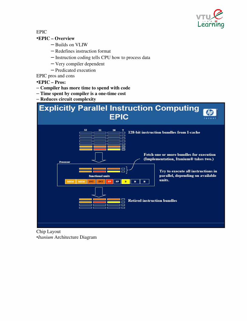
EPIC
•EPIC – Overview
– Builds on VLIW
– Redefines instruction format
– Instruction coding tells CPU how to process data
– Very compiler dependent
– Predicated execution
EPIC pros and cons
•EPIC – Pros:
– Compiler has more time to spend with code
– Time spent by compiler is a one-time cost
– Reduces circuit complexity
Chip Layout
•Itanium Architecture Diagram

•
Itanium Specs
•4 Integer ALU's
•4 multimedia ALU's
•2 Extended Precision FP Units
•2 Single Precision FP units
•2 Load or Store Units
•3 Branch Units
•10 Stage 6 Wide Pipeline
•32k L1 Cache
•96K L2 Cache
•4MB L3 Cache(extern)þ
•800Mhz Clock
Intel Itanium •800 MHz
•10 stage pipeline
•Can issue 6 instructions (2 bundles) per cycle
•4 Integer, 4 Floating Point, 4 Multimedia, 2 Memory, 3 Branch Units
•32 KB L1, 96 KB L2, 4 MB L3 caches
•2.1 GB/s memory bandwidth

Itanium2 Specs
•6 Integer ALU's
•6 multimedia ALU's
•2 Extended Precision FP Units
•2 Single Precision FP units
•2 Load and Store Units
•3 Branch Units
•8 Stage 6 Wide Pipeline
•32k L1 Cache
•256K L2 Cache
•3MB L3 Cache(on die)þ
•1Ghz Clock initially
–Up to 1.66Ghz on Montvale
Itanium2 Improvements
•Initially a 180nm process
–Increased to 130nm in 2003
–Further increased to 90nm in 2007
•Improved Thermal Management
•Clock Speed increased to 1.0Ghz
•Bus Speed Increase from 266Mhz to 400Mhz

•L3 cache moved on die
–Faster access rate
IA-64 Pipeline Features
•Branch Prediction
–Predicate Registers allow branches to be turned on or off
–Compiler can provide branch prediction hints
•Register Rotation
–Allows faster loop execution in parallel
•Predication Controls Pipeline Stages
Cache Features
•L1 Cache
–4 way associative
–16Kb Instruction
–16Kb Data
•L2 Cache
–Itanium
•6 way associative
•96 Kb
–Itanium2
•8 way associative
•256 Kb Initially
–256Kb Data and 1Mb Instruction on Montvale!
Cache Features
•L3 Cache
–Itanium
•4 way associative
•Accessible through FSB
•2-4Mb
–Itanium2
•2 – 4 way associative
•On Die
•3Mb
–Up to 24Mb on Montvale chips(12Mb/core)!
Register
Specification
�128, 65-bit General Purpose Registers
�128, 82-bit Floating Point Registers
�128, 64-bit Application Registers
�8, 64-bit Branch Registers
�64, 1-bit Predicate Registers
Register Model
�128 General and Floating Point Registers
�32 always available, 96 on stack

�As functions are called, compiler allocates a specific number of local and output
registers to use in the function by using register allocation instruction “Alloc”.
�Programs renames registers to start from 32 to 127.
�Register Stack Engine (RSE) automatically saves/restores stack to memory when
needed
�RSE may be designed to utilize unused memory bandwidth to perform register spill and
fill operations in the background
Register Stack
On function call, machine shifts register window such that previous output registers
become new locals starting at r32

�Registers
Instruction
Encoding
=

Five execution unit
slots
Possible Template Values
Figure G.7 The 24 possible template values (8 possible values are reserved) and the instruction slots and stops for each format. Stops are indicated by heavy lines
Straightforward MIPS code
Loop: L.D F0,0(R1) ;F0=array element
ADD.D F4,F0,F2 ;add scalar in F2
S.D F4,0(R1) ;store result

DADDUI R1,R1,#-8 ;decrement pointer
;8 bytes (per DW)
BNE R1,R2,Loop ;branch R1!=R2
The code scheduled to minimize the number of bundles
The code scheduled to minimize the number of cycles assuming one bundle executed
per cycle
Unrolled loop after it has been scheduled for
the pipeline
Loop: L.D F0,0(R1)
L.D F6,-8(R1)
L.D F10,-16(R1)
L.D F14,-24(R1)

ADD.D F4,F0,F2
ADD.D F8,F6,F2
ADD.D F12,F10,F2
ADD.D F16,F14,F2
S.D F4,0(R1)
S.D F8,-8(R1)
DADDUI R1,R1,#-32
S.D F12,16(R1)
S.D F16,8(R1)
BNE R1,R2,Loop
Instruction Encoding
•Each instruction includes the opcode and three operands
•Each instructions holds the identifier for a corresponding Predicate Register
•Each bundle contains 3 independent instructions
•Each instruction is 41 bits wide
•Each bundle also holds a 5 bit template field
Distributing Responsibility
�ILP Instruction Groups
�Control flow parallelism
Parallel comparison
Multiway branches
�Influencing dynamic events
Provides an extensive set of hints that the compiler uses to tell the
hardware about likely branch behavior (taken or not taken, amount to fetch at branch
target) and memory operations (in what level of the memory hierarchy to cache data).
Predication
compare
IA64
compare
then (p1)
else (p2)
p1 p2
Tranditional
Execute multiple paths simultaneously
Reduces mispredicted branches
C code: if( condition ) { … } else { … } …

�Use predicates to eliminate branches, move instructions across branches
�Conditional execution of an instruction based on predicate register (64 1-bit predicate
registers)
�Predicates are set by compare instructions
�Most instructions can be predicated – each instruction code contains predicate field
�If predicate is true, the instruction updates the computation state; otherwise, it behaves
like a nop
Scheduling and Speculation • Basic block: code with single entry and exit, exit point can be multiway
branch
• Control Improve ILP by statically move ahead long latency code blocks.
• path is a frequent execution path
• Schedule for control paths
• Because of branches and loops, only small percentage of code is executed
regularly
• Analyze dependences in blocks and paths
• Compiler can analyze more efficiently - more time, memory, larger view of
the program
• Compiler can locate and optimize the commonly executed blocks
Control speculation
� Not all the branches can be removed using predication.

� Loads have longer latency than most instructions and tend to start time-
critical chains of instructions
� Constraints on code motion on loads limit parallelism
� Non-EPIC architectures constrain motion of load instruction
� IA-64: Speculative loads, can safely schedule load instruction before one or
more prior branches
Control Speculation
�Exceptions are handled by setting NaT (Not a Thing) in target register
�Check instruction-branch to fix-up code if NaT flag set
�Fix-up code: generated by compiler, handles exceptions
�NaT bit propagates in execution (almost all IA-64 instructions)
�NaT propagation reduces required check points
Speculative Load
� Load instruction (ld.s) can be moved outside of a basic block even if branch target
is not known
� Speculative loads does not produce exception - it sets the NaT
� Check instruction (chk.s) will jump to fix-up code if NaT is set
Data Speculation
� The compiler may not be able to determine the location in memory being
referenced (pointers)
� Want to move calculations ahead of a possible memory dependency
� Traditionally, given a store followed by a load, if the compiler cannot
determine if the addresses will be equal, the load cannot be moved ahead of the
store.
� IA-64: allows compiler to schedule a load before one or more stores
� Use advance load (ld.a) and check (chk.a) to implement
� ALAT (Advanced Load Address Table) records target register, memory
address accessed, and access size
Data Speculation 1. Allows for loads to be moved ahead of stores even if the compiler is unsure if
addresses are the same
2. A speculative load generates an entry in the ALAT
3. A store removes every entry in the ALAT that have the same address
4. Check instruction will branch to fix-up if the given address is not in the ALAT
Ld.aAdd
entries
Reg# Add#StoreRemoveentries
Check
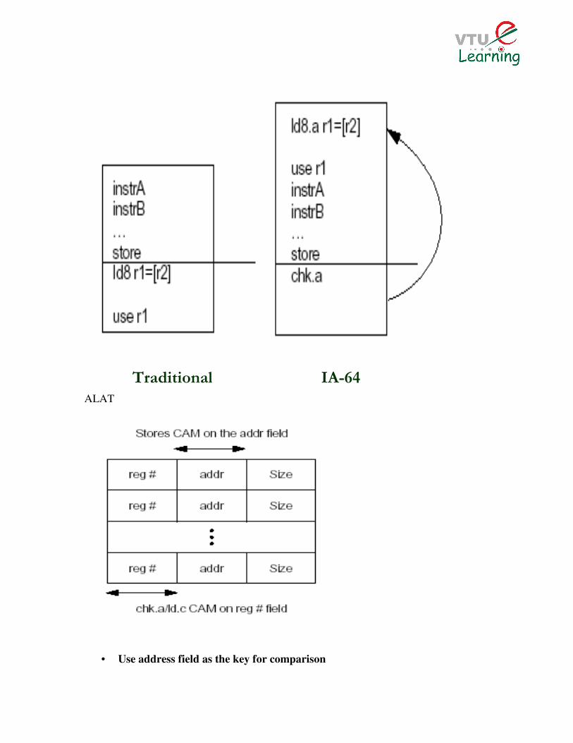
ALAT
• Use address field as the key for comparison
Traditional IA-64

• If an address cannot be found, run recovery code
• ALAT are smaller and simpler implementation than equivalent structures
for superscalars
Register Model
�128 General and Floating Point Registers
�32 always available, 96 on stack
�As functions are called, compiler allocates a specific number of local and output
registers to use in the function by using register allocation instruction “Alloc”.
�Programs renames registers to start from 32 to 127.
�Register Stack Engine (RSE) automatically saves/restores stack to memory when
needed
�RSE may be designed to utilize unused memory bandwidth to perform register spill and
fill operations in the background
Register Stack
On function call, machine shifts register window such that previous output registers
become new locals starting at r32 Software Pipelining
�loops generally encompass a large portion of a program’s execution time, so it’s
important to expose as much loop-level parallelism as possible.
�Overlapping one loop iteration with the next can often increase the parallelism.
Software Pipelining

We can implement loops in parallel by resolve some problems.
�Managing the loop count,
�Handling the renaming of registers for the pipeline,
�Finishing the work in progress when the loop ends,
�Starting the pipeline when the loop is entered, and
�Unrolling to expose cross-iteration parallelism.
•IA-64 gives hardware support to compilers managing a software pipeline
•Facilities for managing loop count, loop termination, and rotating registers
“The combination of these loop features and predication enables the compiler to generate
compact code, which performs the essential work of the loop in a highly parallel form.”
![Cse Viii Advanced Computer Architectures [06cs81] Notes](https://static.fdocuments.in/doc/165x107/55cf8557550346484b8cf5b6/cse-viii-advanced-computer-architectures-06cs81-notes.jpg)