Advanced Compilers Data Flow Analysis Background Theoryplas.cnu.ac.kr/courses/2017f/a_compilers/ac...
39
1 Advanced Compilers Data Flow Analysis – Background Theory Fall. 2017 Chungnam National Univ. Eun-Sun Cho
Transcript of Advanced Compilers Data Flow Analysis Background Theoryplas.cnu.ac.kr/courses/2017f/a_compilers/ac...

1
Advanced CompilersData Flow Analysis – Background
TheoryFall. 2017
Chungnam National Univ.
Eun-Sun Cho

States and Paths
• States
– Consists of the values of all the variables
– The execution of a program can be viewed as a series of
transformations of the program state
– Each execution of an intermediate code statement transforms an input
state to a new output state
• Input state : associated with the program point before the statement
• Output state : associated with the program point after the statement
• Execution path from point p1 to point pn to be a sequence of
points p1, p2,… pn such that for each i = 1, 2, …n-1, either
– pi is the point immediately preceding a statement and pi+1 is the point
immediately following that same statement, or
– pi is the end of some block and pi+1 is the beginning of a successor
block 2

There is an infinite number of possible execution paths through a program
– There is no finite upper bound on the length of an execution path
(1,2,3,4,9) (1,2,3,4,5,6,7,8,3,4,9) (1,2,3,4,5,6,7,8,3,4,5,6,7,8,3,4,9)…3
d1 : a = 1
if read() <=0 goto B4
d2 : b = a
d3 : a = 243
goto B2
(1)
(2)
(3)
(4)
(5)
(6)
(7)
(8)
(9)
B1
B2
B3
B4

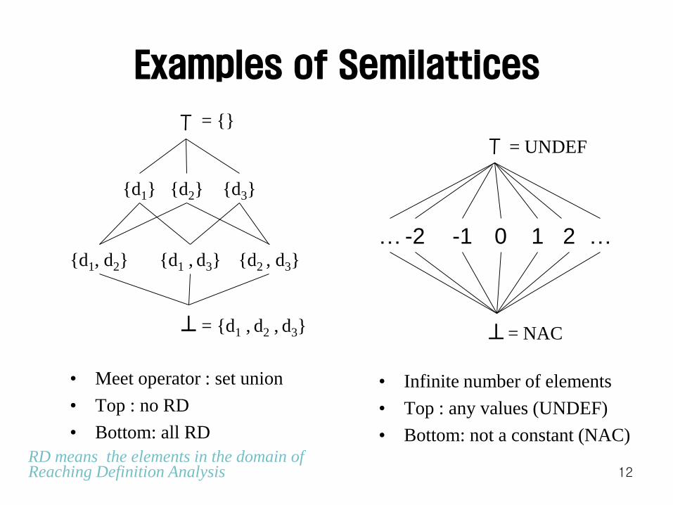
Data Flow Analysis – Basic Concepts
• Dataflow analysis has a unified theory.
• Basic concepts
– Data flow information:
• represented as semilattice
– Data flow functions:
• model effect of basic blocks
– Data flow equations:
• relations of control flow and effects of basic blocks
– Data flow solutions: (finally!)
4

Dataflow Values
• Dataflow values
– Abstraction of set of all possible program states that can be observed
for that point
– A domain means the set of “possible dataflow values”
• Eg. The domain of dataflow values for reaching definitions is the
set of all subsets of definitions in the program
5

Semilattices
Semi-lattice L for representing DFA information;
– L is an algebraic structure L , , T
– L consists of a set of values: L={x1, x2,...}
• L might have infinite number of elements
– L has a meet operator z=x y, where x, y, z L
– Two unique elements of L: , T (bottom, top)
– Height of semi-lattice is finite
– L can be an algebraic product:
• L= L1 L2 .... Lk
6

Properties of Meet Operator
• For all x, y L, there exists a unique z L s.t. z=x y
(closure)
• For all x,y L: x y = y x (commutativity)
• For all x,y,z L: (x y) z = x (y z) (associativity)
• For all x L, (x ) =
• For all x L, (x T) = x
7

Example
• Consider as
– x y is unique
– x y is y x
– (x y) z = x (y z)
– (x {} ) = {} ( is {})
– (x U ) = x, when U is universe (T is U)
• Consider as
– x y is unique
– x y is y x
– (x y) z = x (y z)
– (x U ) = U ( is U)
– (x {} ) = x (T is {})
8

Partial Ordering and Meet Operator
• Meet operator induces a partial order ( ) on values in
L:
– x y x y = x
– Note that we usually do in the opposite way ; define (that is, g.l.b.)
from a given
• Strict partial order
– x y x y = x and x y
• Height of L
– the length of the longest strictly ascending chain
– the maximal n s.t. there ,…, exist x1, x2 , …, xn s.t.
x1 x2 … xn T9
Example
• Consider as
– x y x y = x ( is )
• Consider as
– x y x y = x ( is )
10

Note: Partial Ordering
• Partial order
– If x y then value x has less information than value y.
• Properties of partial ordering
– Reflexivity (for all x, x x)
– Antisymmetry (if x y and y x, then x = y)
– Transitivity (if x y and y z, then x z)
11
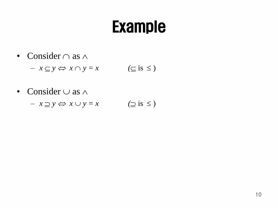
Examples of Semilattices
• Infinite number of elements
• Top : any values (UNDEF)
• Bottom: not a constant (NAC)
12
{d1} {d2} {d3}
{d1, d2} {d2 , d3}{d1 , d3}
= {d1 , d2 , d3}
T = {}
• Meet operator : set union
• Top : no RD
• Bottom: all RD
RD means the elements in the domain of Reaching Definition Analysis
-2 -1 0 1 2 ……
T
= NAC
= UNDEF

Set As a Bit Vector
13
<1,0,0> <0,1,0> <0,0,1>
<1,1,0> <0,1,1><1,0,1>
= <1,1,1>
T = <0,0,0>
• Meet operator : bitwise
• Top : <0,0,0>
• Bottom: <1,1,1>
{d1} {d2} {d3}
{d1, d2} {d2 , d3}{d1 , d3}
= {d1 , d2 , d3}
T = {}
• Meet operator : set union
• Top : no RD
• Bottom: all RD
previous examplebit vector
representation
Efficient representation

Then,
why do we use semilattice as dataflow values?
The answer will be shown later on...
14
Data Flow Analysis – Basic Concepts
• Dataflow analysis is a unified theory.
• Basic concepts
– Data flow information:
• represented as semilattice
– Data flow functions:
• model effect of basic blocks
– Data flow equations:
• relations of control flow and effects of basic blocks
– Data flow solutions: (finally!)
15
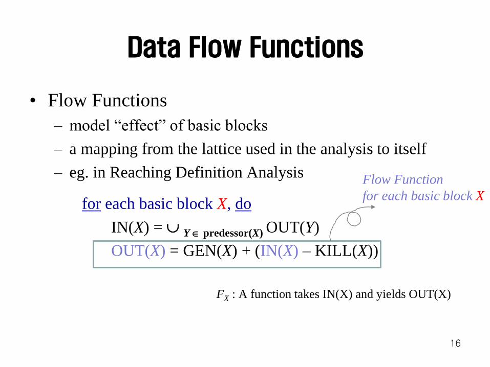
Data Flow Functions
• Flow Functions
– model “effect” of basic blocks
– a mapping from the lattice used in the analysis to itself
– eg. in Reaching Definition Analysis
for each basic block X, do
IN(X) = Y predessor(X) OUT(Y)
OUT(X) = GEN(X) + (IN(X) – KILL(X))
FX : A function takes IN(X) and yields OUT(X)
16
Flow Function
for each basic block X

17
receive m (val)
f0 0
f1 1
return m
m <= 1
i 2
i <= m
return f2f2 f0 + f1
f0 f1
f1 f2
i i+1
1
2
3
4
8
9
10
11
N Y
Bit
Position
Definition Basic
Block
1 m in node 1 B1
2 f0 in node 2
3 f1 in node 3
4 i in node 5 B3
5 f2 in node 8 B6
6 f0 in node 9
7 f1 in node 10
8 i in node 11
B1
B6FB1(<x1x2x3x4x5x6x7x8>)=<111x4x500x8>
FB6(<x1x2x3x4x5x6x7x8>)=<x10001111>
B3

Data Flow Analysis – Basic Concepts
• Dataflow analysis is a unified theory.
• Basic concepts
– Data flow information:
• represented as semilattice
– Data flow functions:
• model effect of basic blocks
– Data flow equations:
• relations of control flow and effects of basic blocks
– Data flow solutions: (finally!)
18

Equations for Iterative Analysis
• in(B) = Init , for B = entry
Q Pred(B) out(Q) , otherwise
• out(B) = FB(in(B))
or
• in(B) = Init , for B = entry
Q Pred(B) FQ(in(Q)) , otherwise
• Solution : actually undecidable
19

Data Flow Analysis – Basic Concepts
• Dataflow analysis is a unified theory.
• Basic concepts
– Data flow information:
• represented as semilattice
– Data flow functions:
• model effect of basic blocks
– Data flow equations:
• relations of control flow and effects of basic blocks
– Data flow solutions: (finally!)
20

MOP: Meet-Over-All Paths
• The problem of deciding if an arbitrary path in a
program is executable is undecidable
– Program analysis is commonly performed under the
assumption that “all paths in the program are executable”
• MOP (meet-over-all-paths)
– for every path in the flow graph is taken,
– MOP(B) = p Path(B) Fp(Init) , for each block B
– where Fp = FBn …. FB1, for B1 =entry, … , Bn=B
21

Hard to Solve the Equations for MOP : Why?
• out(B2) = FB2(in(B2)) = FB2 ( Q Pred(B2) FQ(in(Q)) )
= FB2 (FB1(in(B1)) FB3(in(B3)))
= FB2 (FB1(Init) FB3(in(B3)))
since in(B3) = Q Pred(B3) FQ(in(Q)) = FB2(in(B2))
FB2(in(B2)) = FB2 (FB1(Init) FB3(FB2(in(B2) ))
out(B2) = FB2 (FB1(Init) FB3(out(B2))
22
B2
B1(Entry)
B3
“What we want to know” (the estimated state after B2)
“What-we-want-to-know” is defined by “what-we-want-to-know” itself.
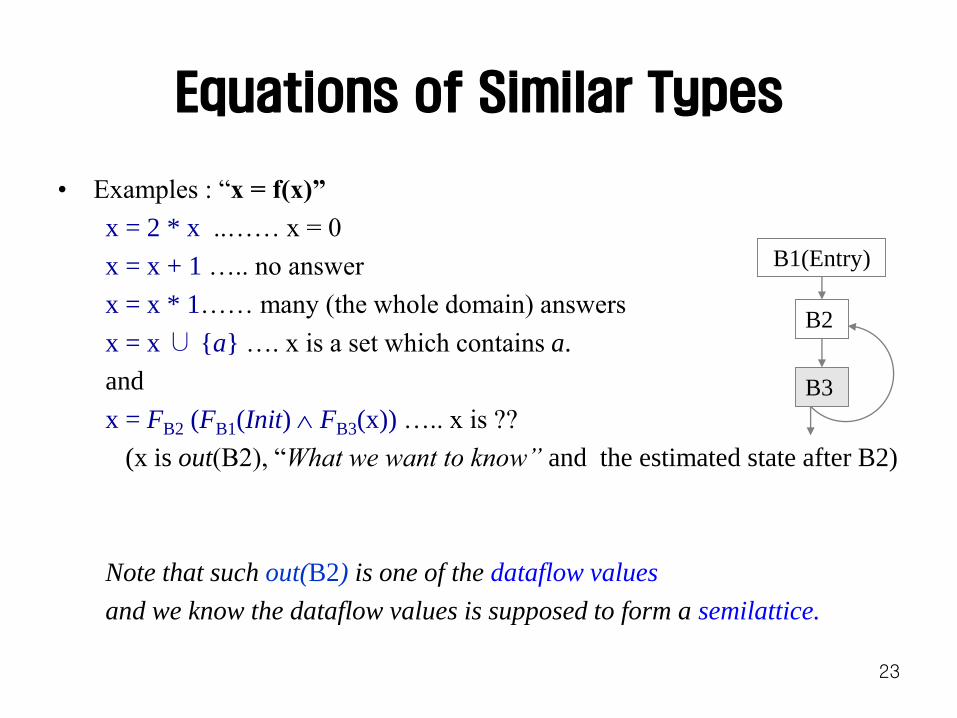
Equations of Similar Types
• Examples : “x = f(x)”
x = 2 * x ..…… x = 0
x = x + 1 ….. no answer
x = x * 1…… many (the whole domain) answers
x = x ∪ {a} …. x is a set which contains a.
and
x = FB2 (FB1(Init) FB3(x)) ….. x is ??
(x is out(B2), “What we want to know” and the estimated state after B2)
Note that such out(B2) is one of the dataflow values
and we know the dataflow values is supposed to form a semilattice.
23
B2
B1(Entry)
B3

Approximated Solution - MFP
• MFP -Maximal
Fixed Point solution
an iterative
algorithm
visit and evaluate
in/out of each B
from an initial
value
do again and
again until there
is no change
24
initialize IN(X) = for all basic blocks X
initialize OUT(X) = GEN(X) for all basic blocks X
change = 1
while (change) do
change = 0
for each basic block X, do
old_OUT = OUT(X)
IN(X) = Y predessor(X) OUT(Y)
OUT(X) = GEN(X) + (IN(X) – KILL(X))
if (old_OUT != OUT(X)) then
change = 1
endif
endfor
endfor eg. Reaching Definition Analysis

In MFP Algorithm - Intuitive Idea
• For all X, OUT(X) is a set of RD, that is, a
semilattice!
– for all X, OUT(X) only increases (or remains the same)
while the analysis is going
• Even along the longest chain, it grows and grows until it
reaches (after a finite number of iteration, by the
definition of semilattice,) And it is not able to increase
further, so will remain the same.
• Or it will stop somewhere in the middle of the DAG, and
remains the same.
• This is why we chose the semilattice with finite height as
the domain of dataflow values, which guarantees that the
finite number of iteration will give an answer, when it only
grows.
25How can we prove it? (need more theory)

MFP – More Theory (1)
• “How can we know that OUT(B) is always increasing?”
• Consider following definitions of monotone functions
– (Monotone functions) : a function f is monotone, for all x, y, x y
implies f(x) f(y)
– “For a monotone function, f () < f f () is always true.”
• Proof) < f (), since is the bottom, the lowest element.
• f () < f f (), since f is monotone.
– “If we consider FB (X) = GEN(B) ∪ (X – KILL(B)), it is monotone.”
• Proof Sketch)
• For X1, X2, s.t. X1 < X2, it is true that C + (X1 -D) < C + (X2 -D).
• Thus FB (X1) < FB (X2) , from these two facts.
26
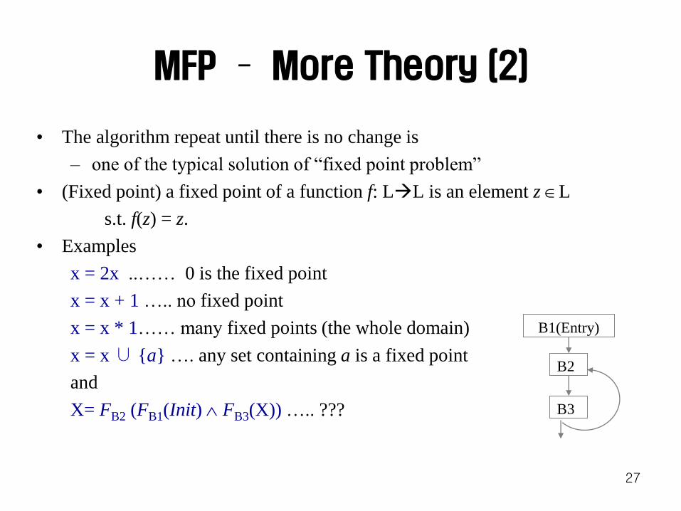
MFP – More Theory (2)
• The algorithm repeat until there is no change is
– one of the typical solution of “fixed point problem”
• (Fixed point) a fixed point of a function f: LL is an element z L
s.t. f(z) = z.
• Examples
x = 2x ..…… 0 is the fixed point
x = x + 1 ….. no fixed point
x = x * 1…… many fixed points (the whole domain)
x = x ∪ {a} …. any set containing a is a fixed point
and
X= FB2 (FB1(Init) FB3(X)) ….. ???
27
B2
B1(Entry)
B3

MFP – More Theory (3)
• (Distributive) f(x y) = f(x) f(y)
• (LF ) LF is a set of all monotone functions from L to L
• (f n ) For any f LF, f n is defined by
f 0 = id and
for n 1, f n = f f n-1 Note that f g (x) = f(g(x))
• (Fix f) Fix f is {f n | n >= 0} for distributive f LF
in other words, “if f is continuous ccpo (chain complete partial ordering)”
actually T instead of for meet operator •
• FIXED POINT THEORM “Fix f is the least fixed point of f” (..believe it!)
– it stops and it is the minimum!
– it is also true when f is FB(X) = GEN(B) ∪ (X – KILL(B))
28

MFP Theory (4)
• Example 1. To find out a least fixed point of f(A) = A∪ {a}
to solve equation A = A∪ {a}
step1. apply {}
thus f({}) = {}∪{a} = {a}
step 2. apply f({})
thus f(f({})) = {a} ∪{a} = {a}
since this will not change further, {a} is the least fixed point of f(A)= A∪ {a}
• Example 2. To solve X= FB2 (FB1(Init) FB3(X)) ... when X is OUT(B2)
step1. apply {}
thus f({}) = FB2 (FB1(Init) FB3({}))
step2. apply f({})
thus f(f({})) = FB2 (FB1(Init) FB3(FB2 (FB1(Init) FB3({})) ))
step 3. apply f(f({})) .....
29
B2
B1(Entry)
B3
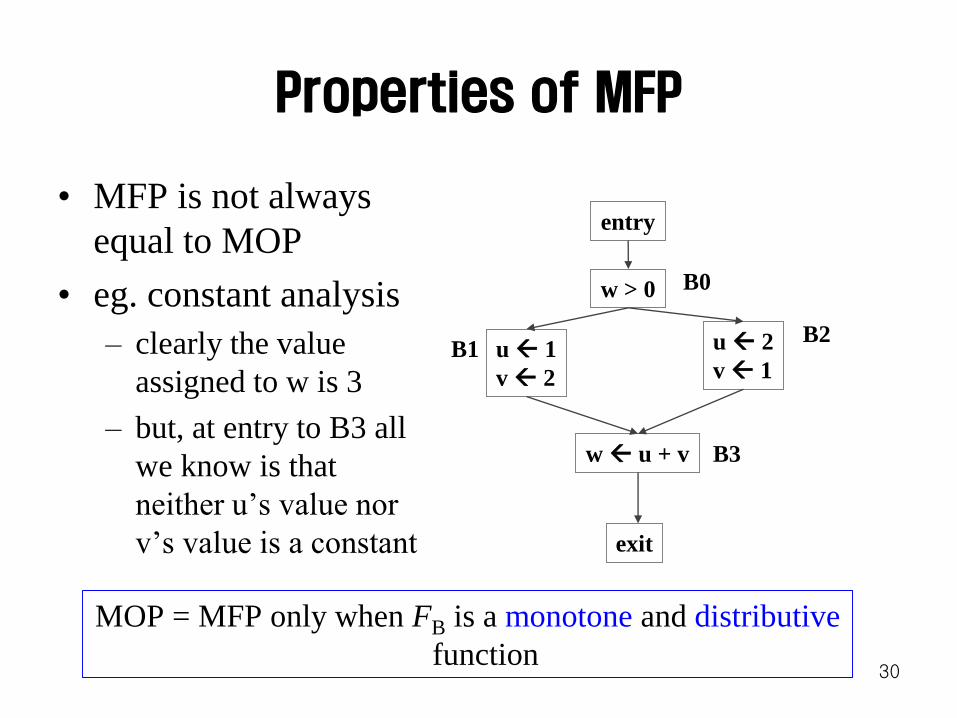
Properties of MFP
• MFP is not always
equal to MOP
• eg. constant analysis
– clearly the value
assigned to w is 3
– but, at entry to B3 all
we know is that
neither u’s value nor
v’s value is a constant
30
entry
w > 0
u 1
v 2
u 2
v 1
w u + v
exit
B1
B0
B2
B3
MOP = MFP only when FB is a monotone and distributive
function

Properties of MFP (More)
• Distributive) f(x y) = f(x) f(y)
• FB:
– If s is not an assignment statement, then FB is the identity
function
– If s is an assignment (x = ..) ,
• RHS of s is constant … emit x c
• RHS of s is y + z is emit x const if both y and z are const
– NAC, if one of them is NAC (… )
– UNDEF, otherwise (… T)
31
FB3(FB1 (m0) FB2 (m0)) FB3 (FB1 (m0)) FB3 (FB2 (m0))
FB3(FB1 (m0) FB2 (m0)) < FB3 (FB1 (m0)) FB3 (FB2 (m0))
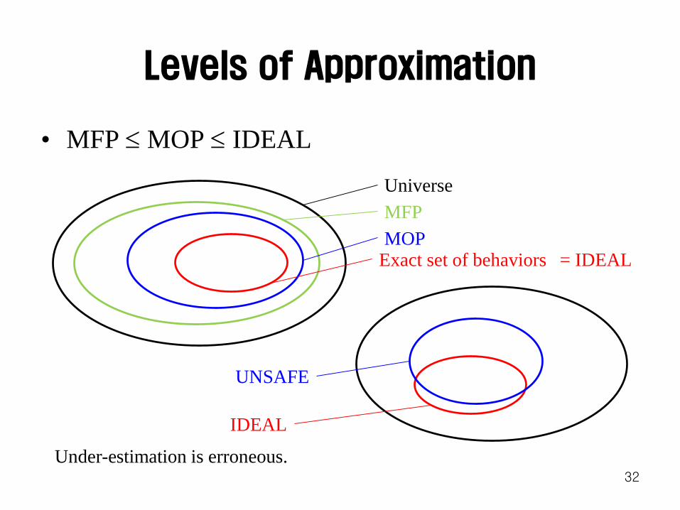
Levels of Approximation
• MFP MOP IDEAL
32
= IDEALMOP
MFP
Universe
Exact set of behaviors
IDEAL
UNSAFE
Under-estimation is erroneous.
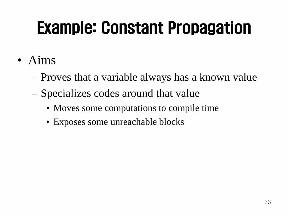
Example: Constant Propagation
• Aims
– Proves that a variable always has a known value
– Specializes codes around that value
• Moves some computations to compile time
• Exposes some unreachable blocks
33
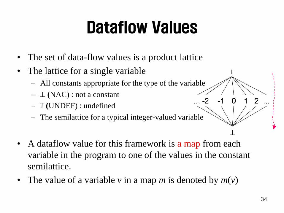
Dataflow Values
• The set of data-flow values is a product lattice
• The lattice for a single variable
– All constants appropriate for the type of the variable
– (NAC) : not a constant
– T (UNDEF) : undefined
– The semilattice for a typical integer-valued variable
• A dataflow value for this framework is a map from each
variable in the program to one of the values in the constant
semilattice.
• The value of a variable v in a map m is denoted by m(v)
34

35
• fs : the transfer function of statement s
• If s is not an assignment statement, then fs is simply the
identity function
• If s is an assignment to variable x, then
• m’(v) = m(v), for all variables v x, where m’ = fs (m)
(a) If the RHS of the statement s is a constant c, then m’(x) = c
(b) If the RHS is of the form y+z ,then
m’(x) = m(y) + m(z) if m(y) and m(z) are constant values
NAC if either m(y) or m(z) is NAC
UNDEF otherwise
(c) If the RHS is any other expression (e.g. a function call or assignment
through a pointer), then m’(x) = NAC
Transfer Function

Monotonicity of Transfer Function
• In case (b), each possible
input value of y, the value of x
does not get bigger as the
value of z gets smaller :
monotone
• Otherwise, fs either does not
change the value of m(x), or it
changes the map to return a
constant or NAC : monotone
36
m(y) m(z) m’(x)
UNDEF
(T)
UNDEF UNDEF
c2 UNDEF
NAC NAC
c1 UNDEF UNDEF
c2 c1+c2
NAC NAC
NAC
()
UNDEF NAC
c2 NAC
NAC NAC
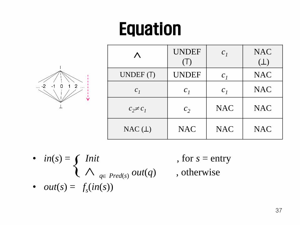
Equation
37
UNDEF
(T)
c1 NAC
()
UNDEF (T) UNDEF c1 NAC
c1 c1 c1 NAC
c2 c1 c2 NAC NAC
NAC () NAC NAC NAC
• in(s) = Init , for s = entry
q Pred(s) out(q) , otherwise
• out(s) = fs(in(s))

Notes
• Initial value : m0(v) = T (UNDEF) for all variable v
– 프로그램이진행해가면서 NAC() 가많아진다
– 더이상변화가없을때까지반복한다.
• As long as there exists a path that defines a variable
reaching a program point, the variable will not have an
UNDEF value
38

review Nondistributivity
39
fB3(fB1 (m0) fB2 (m0)) < fB3 (fB1 (m0)) fB3 (fB2 (m0))
Nondistributivity
f(x y) f(x) f(y)
• clearly the value
assigned to w is 3
• but, at entry to B3 all we
know is that neither u’s
value nor v’s value is a
constant
• MFP but not MOP!
B1