ADVANCED BIOENGINEERING METHODS LABORATORY OPTICAL TRAPPING · ADVANCED BIOENGINEERING METHODS...
25
ADVANCED BIOENGINEERING METHODS LABORATORY OPTICAL TRAPPING Aleksandra Radenovic 1 OPTICAL TRAPPING ABSTRACT Optical trap is a powerful tool used currently in many physical and biological applications. It allows for instance to manipulate and measure with high precision different cellular structure in biophysics and also to perform some experiments in biology such as cell sorting, singl e cell analysis…In this lab, the objectives are twice: i) To become familiar with the fundamentals of optical trapping and ii) To learn how to calibrate the optical traps for position detection and force measurement. Thus it will start with a brief theory on optical trapping system and the controls for it. Then the subsequent practical work will be as following: Load a sample slide into the trap for calibrating the position detector, and find a bead attached to the coverglass surface. Run the Matlab position calibration to relate the voltage output of the position detector to bead displacement in nanometers. Make a new slide with free beads, find bead that is not attached to the surface and trap it. Use two different methods to calculate the trap stiffness and compare their results. Finally, the data generated will be analysed using Matlab.
Transcript of ADVANCED BIOENGINEERING METHODS LABORATORY OPTICAL TRAPPING · ADVANCED BIOENGINEERING METHODS...

ADVANCED BIOENGINEERING METHODS LABORATORY
OPTICAL TRAPPING
Aleksandra Radenovic
1
OPTICAL TRAPPING
ABSTRACT
Optical trap is a powerful tool used currently in many physical and biological applications It allows for
instance to manipulate and measure with high precision different cellular structure in biophysics and also to
perform some experiments in biology such as cell sorting single cell analysishellipIn this lab the objectives are
twice i) To become familiar with the fundamentals of optical trapping and ii) To learn how to calibrate the
optical traps for position detection and force measurement Thus it will start with a brief theory on optical
trapping system and the controls for it Then the subsequent practical work will be as following Load a sample
slide into the trap for calibrating the position detector and find a bead attached to the coverglass surface Run
the Matlab position calibration to relate the voltage output of the position detector to bead displacement in
nanometers Make a new slide with free beads find bead that is not attached to the surface and trap it Use two
different methods to calculate the trap stiffness and compare their results Finally the data generated will be
analysed using Matlab
ADVANCED BIOENGINEERING METHODS LABORATORY
OPTICAL TRAPPING
Aleksandra Radenovic
2
TABLE OF CONTENTS
1 Theoryhelliphelliphelliphelliphelliphelliphelliphelliphelliphelliphelliphelliphelliphelliphelliphelliphelliphelliphelliphelliphelliphelliphelliphelliphelliphelliphelliphelliphelliphelliphelliphelliphelliphelliphellip3
11 History 3
12 The Physics behind Trapping 3
13 Quantitative measurements 9
14 Optical Tweezers - Setup Description 10
15 Questions (Theory) 15
2 Practical workhelliphelliphelliphelliphelliphelliphelliphelliphelliphelliphelliphelliphelliphelliphelliphelliphelliphelliphelliphelliphelliphelliphelliphelliphelliphelliphelliphelliphelliphelliphellip15
21 Material requirements 15
22 Polystyrene suspensions preparation 15
23 Floating bead preparation 16
24 Slide loading 17
25 Trapping bead 17
26 Calibration 20
27 Measurement of the trap stiffness 22
3 Data analysishelliphelliphelliphelliphelliphelliphelliphelliphelliphelliphelliphelliphelliphelliphelliphelliphelliphelliphelliphelliphelliphelliphelliphelliphelliphelliphelliphelliphelliphelliphelliphellip24
4 Referenceshelliphelliphelliphelliphelliphelliphelliphelliphelliphelliphelliphelliphelliphelliphelliphelliphelliphelliphelliphelliphelliphelliphelliphelliphelliphelliphelliphelliphelliphelliphelliphelliphellip25
ADVANCED BIOENGINEERING METHODS LABORATORY
OPTICAL TRAPPING
Aleksandra Radenovic
3
I THEORY
Optical trap or tweezers is a device used to apply piconewton sized forces and make precise measurements
on a scale of roughly one micron It can be created by applying a precisely focused laser onto a dielectric
material It allows scientists to make very detailed manipulations and measurements on several objects in the
field of cell biology and thus acts as a major tool in biophysics They are used in biological experiments ranging
from cell sorting to the unzipping of DNA and also in physical applications such as atom cooling
11 History
The effect of light on matter has been known for over four hundred years dating from Kepler‟s observation
that comet tails always point away from the sun Indeed light from the sun can exert a pressure up to 5 mNm2
on a totally reflecting surface ten orders of magnitude less than the force on a cube of the same dimensions due
to gravity on the earth‟s surface Although resulting in an extremely small force radiation pressure from
sunlight can be significant for example as the driving force behind solar sails where gravity is negligible At
the beginning of the twentieth century using thin plates suspended in a evacuated radiometer Lebedev 1 was
the first to experimentally measure the radiation pressure proposed by Maxwell-Bartoli showing that the
pressure for a reflective surface is twice that of an absorbing surface Arthur Ashkin 2-4
discovered the method of
optical trapping in 1970 He calculated that the momentum from a high power laser focused entirely onto a
micron bead would propel the bead forward with 100000 gs of acceleration Taken by curiosity he performed
this experiment and found that not only was the intended bead pushed downstream by the laser but also that
other beads in his solution were highly attracted to the beam-path and flew in laterally from other parts of his
slide He then created the first working trap by using two opposing laser beams
At one point a bacterium that had contaminated a sample flew into the trap and was trapped 5 thus instigating
the traps revolutionary use in cell biology Today optical traps are used extensively in both atom-trapping
experiments and in biophysics labs worldwide The focus for this laboratory section is on the basic science
behind how force is generated in an optical trap and how it can be calibrated and used to characterize the force
spectroscopy of biomolecules
12 The Physics behind Trapping
The interaction between light and matter is a complicated one which is not understood fully for all cases but
informative approximations are available under a number of limits The origin of a force on matter because of
an electromagnetic wave can be understood qualitatively by an electric field exerting a force on charges within
a particle and a magnetic field exerting a force on currents
121 Gradient force
Light incident on a particle creates a dielectric response due to the polarizability of the constituent atoms or
ions For one of these atoms or ions in a monochromatic linearly polarized continuous light field E the time-
averaged induced dipole moment is
ADVANCED BIOENGINEERING METHODS LABORATORY
OPTICAL TRAPPING
Aleksandra Radenovic
4
p E (01)
For a small particle in an aqueous medium where 2
2 3
2
1
2
cm
c
ni n
n
is the relative complex
polarizability of the particle to the surrounding medium (nm is medium refractive index and nc is relative index
of the particle np to the index of the surrounding medium nm ) The interaction of the induced dipole with the
electric field of the light creates an electrostatic potential
U p E (02)
Thus in a light field with a spatially varying intensity there is a gradient
( )gradF U p E E E (03)
For a small particle of radius rp this leads to the force relation
3 3 2
2
2
1
2 2
m p cgrad
c
n r nF E
n
(04)
Thus the gradient force is linearly dependent on the spatial variation of the intensity of the light field and on
the dielectric contrast of the particle to be trapped relative to the surrounding media which can be described by
the Clausius-Mossotti relation For particles with a refractive index higher than the surrounding medium the
gradient force acts toward the point of highest intensity that is to say the focal point of a diffraction-limited
beam in optical tweezers Conversely particles with a lower refractive index can be trapped at a minimum in
the light field intensity The strength of the restoring gradient force in an optical trap of radius r can be
characterized as a Hookean spring with stiffness k where the force is linearly proportional to small
displacements (d lt r2)
F r (05)
The laser trap produced by a focused Gaussian beam can be classified by an almost harmonic potential For a
m particle in viscous fluid the friction force is ordered of magnitude larger than the inertial force The particle
shows an exponential dumped motion
0( ) exp6
x t x t
(06)
With the trap period a measure of correlation time is given
6 pr
(07)
ADVANCED BIOENGINEERING METHODS LABORATORY
OPTICAL TRAPPING
Aleksandra Radenovic
5
Where is the viscosity of the surrounding medium is the trap stiffness and rp is friction constant according
to the Stoke‟s law A schematic of the axial and radial potentials and their resulting stiffness‟s is shown in
Figure 1 Techniques for measuring the stiffness of an optical trap are described later but for a 1 m diameter
polystyrene bead in a typical optical tweezers setup the stiffness can be varied easily in the range 10minus6
minus01
pNnm by adjusting the laser power from 10ndash1000 mW These characteristics complement the stiffness of
physical cantilevers such as AFM tips (10ndash104 pNnm) which cannot be as easily tuned after fabrication
Figure 1 (a) The axial and radial trapping potentials of a bead in an optical trap lead to (b) differing stiffnesses and extents (c)
With the addition of the scattering force the trap center is offset from the focal point
The trap stiffness is important in determining the minimum force which can be measured through
displacement detection and sets an upper limit for the maximum useful sampling rate through the trap
frequency Although not immediately obvious from these simple expressions the trap stiffness is greatest when
the particle to be trapped is the same size as the beam waist as particle size decreases the restoring force
decreases rapidly but decreases only modestly when the particle size increases
122 Scattering force
The second force component in an optical trap arises from the scattering of light and is a consequence of
photons having momentum This force acts in the direction of propagation of the light and is dependent on the
light intensity rather than the gradient The momentum of a single photon of energy E is
mE np k
c
(08)
A beam of incident photons can be scattered from the particle resulting in two impulses one along the
direction of light propagation and the other opposite the direction of the scattered photon For isotropic
ADVANCED BIOENGINEERING METHODS LABORATORY
OPTICAL TRAPPING
Aleksandra Radenovic
6
scattering dependent on the size of the particle the latter impulse has no preferred direction and results in a net
force in the direction of light propagation The change in momentum or force of a particle can be calculated by
considering the photon flux impinging on and leaving an object under the conservation of momentum
m
scat in out
n SnF S S dA
c c
(09)
Where nm is the refractive index of the surrounding medium is the time-averaged Poynting vector c is the
speed of light and s is the particle‟s optical cross section In the case of a small spherical (much smaller than
the wavelength of impinging light) dielectric particle the Rayleigh scattering cross-section is
24 26
2
2 18
3 2
m cp
c
n nr
n
(010)
Where rp is the particle radius nc = np nm is the refractive index contrast between the particle (np) and the
medium (nm) and k = 2πλ is the wave vector of the trapping light The scattering force on a Rayleigh particle
can then be written in terms of the light intensity I0 4
5 6 2
04 2
128 1
3 2
p c mscat
c
r n nF I
n c
(011)
Thus the scattering force is dependent on the photon flux or light intensity the wavelength of the trapping
light the particle size and its refractive index contrast against the liquid in which it is immersed For larger
particles (rp gtgt ) the scattering cross-section can be expressed as 2
scatQ r p where Qscat approaches the
limit of 2
However for intermediate sizes an accurate force estimate needs to be numerically
evaluated using Mie theory 6 in part because the scattering of incident photons is no longer isotropic To
maximize the gradient force the particle‟s radius should be comparable to the wavelength of the trapping laser
and its associated minimum focal spot size and consequently is most appropriately described by the
intermediate Mie regime The need to numerically solve Mie scattering theory is one of the complications in
developing a simple model for optical tweezers and makes direct comparison of the gradient force and
scattering force difficult However one variable which can be controlled and optimized is the refractive index
contrast between the trapped particle and the surrounding medium The optimal refractive index contrast is 12ndash
13 which maximizes the gradient force with respect to the scattering force for the incident
optical power P
Conveniently polystyrene beads in water have a refractive index contrast of nc = 159133 = 12 close to
optimal with a potential maximum force of Fmax = 22 pNmW though optical tweezers generally operate at
around 23 of this value 7
Adding the two force components results in the equilibrium position for an optical trap being displaced a
distance proportional to the light intensity from the minimum beam waist in the direction of the light
propagation typically 100ndash500 nm as illustrated in Figure 1 c This distance can be found experimentally by
max
049 mn PF
c
max
049 mn PF
c
ADVANCED BIOENGINEERING METHODS LABORATORY
OPTICAL TRAPPING
Aleksandra Radenovic
7
translating a trapped bead into a surface and measuring the displacement of the bead in the trap when it is in the
focal plane of the surface or comparing it to a bead previously fixed to the surface
123 Rayleigh Regime (r ltlt )
In the two particle size limits the Rayleigh regime (r ltlt ) and the ray optics regime (r gtgt) a theoretical
treatment for calculating the radiation pressure is relatively straightforward and provides a number of useful
insights In the Rayleigh regime particles can be treated as a collection of dipoles polarized by the envelope of
the light field forming the trap with the phase of the field being approximately constant throughout the particle
In the previous sections equations were presented for the gradient and scattering forces on small dielectric
particles however in practice it is difficult to exert sufficient force to trap a dielectric particle below 100 nm in
size with current optics and laser limitations
The force exerted by the laser is proportional to the particle‟s polarizability which is in turn proportional to the
volume of the trapped object to trap a 10 nm object requires a million times as much input power as to trap a 1-
micron object
As particle size increases the difference between Rayleigh and Mie scattering becomes measurable for
particles larger than 200 nm for visible trapping fields 8 and Rayleigh approximations break down for most
trappable objects The dielectric constant can be enhanced to trap particles down to 5 nm in size by exploiting
nonlinearities such as a plasma resonance ionic resonance or intensity dependent refractive index 9
Alternatively the medium surrounding the particle can be modified to minimize Brownian motion to the
extreme of trapping and cooling small numbers of atoms in an ultrahigh vacuum chamber 10
In general
however the complications and limitations associated with these approaches mean that optical traps rarely
operate in a pure Rayleigh regime and predictions can be inaccurate without experimental validation
124 Ray Optics Regime (r gtgt )
In the other limiting case where the size of the particle to be trapped is much larger than the wavelength of
light and has a small refractive index contrast with the surrounding medium the component forces can be
modeled using ray optics
An incident monochromatic light beam can be decomposed into individual rays with appropriate intensity
momentum and direction In a uniform nondispersive media these rays propagate in a straight line and can be
described by geometric optics For a uniform dielectric sphere the optical forces including the scattering
component can be calculated directly from ray optics 4
2
2
(cos(2 2 ) cos(2 ))1 cos(2 )
1 2 cos(2 )
m F R T Rscat R
T
n P T RF R
c R R
(012)
2
2
(sin(2 2 ) cos(2 ))1 sin(2 )
1 2 cos(2 )
m F R T Rgrad R
T
n P T RF R
c R R
(013)
ADVANCED BIOENGINEERING METHODS LABORATORY
OPTICAL TRAPPING
Aleksandra Radenovic
8
where R amp TF are the Fresnel coefficients and R and T are the angles for reflection and transmission of the
incident rays Figure 2 schematically illustrates the origins of the axial and radial forces due to diffraction and
how the component forces add together
For nonspherical and complex particles approximations can be computed 11
The ray optics regime is
increasingly accurate for dielectric particles of radius 5 c
p
c
nr
n
though for these larger particles the radial
trapping force diminishes However increasing the focal spot size to compensate would decrease the axial
trapping force As mentioned earlier trapping efficiency is highest for objects which are approximately a
wavelength in size and therefore fall in the intermediate regime between the Rayleigh and ray optics regimes
These theoretical models generally assume a continuous diffraction limited monochromatic beam focused by
a high numerical aperture lens to trap a rigid dielectric sphere with a refractive index higher than the
surrounding medium All of these assumptions can be broken through choice of trap geometry light source and
particle to be trapped For the remainder of this section we will consider some of the trap designs light sources
and particles which have been or can be used
Figure 2 Schematic of the optical forces in the ray-optics regime Summing the rays gives an (a) axial force due to vertical
displacement from trap center (b) radial force due to lateral displacement from trap center Taking into account gravity and
scattering (c) the axial and (d) radial gradient force must be the dominant component to form an optical trap
ADVANCED BIOENGINEERING METHODS LABORATORY
OPTICAL TRAPPING
Aleksandra Radenovic
9
In order to trap a particle we need to create a stable equilibrium The force that will be counteracting the
movement in this case is the change in momentum (remember that force is defined to be dpdt) of the laser light
path (light carries momentum) as the trapped particle refracts and bends the light in various ways In order to
understand how it is stable we only need to consider a couple of test cases In the Figure 2 to the right we see
an illustration of two possible laser-particle set-ups The red region represents the laser at its focus point the
blue ball is the particle and the black arrows are representative light rays whose thicknesses correspond to their
intensities (note that the beam is brightest at its center) In case (a) the particle is dead canter and will not be
pushed left or right It is still reflecting some of the laser light hitting it dead on however and may be pushed
downstream
To counter act this force we note that the two beams though now symmetric are still being bent inwards This
slight bending creates a force that pulls the bead back towards the laser source This only happens very near the
focus of the laser and only when the light comes in at an extremely crossed angle or at a high numerical
aperture
In case (b) we see that the particle has been moved slightly to the left the two black arrows refract through the
particle and bend inwards The reactionary force vectors on the particle are also included in the image We see
that because the particle is slightly to the left of center the right ray is more intense (and thus carries more
momentum) than the left ray As a result of the rays bending to the left the particle will be pushed to the right
in order to conserve momentum Thus a perturbation to the left causes a right directed force back towards
equilibrium
If a picture is worth a thousand words then a java applet must be worth a million Inspect this applet to get a
feel of how the light-bending forces work Be sure to adjust the numerical aperture at the bottom in order to
obtain a working trap Also play with following java applet
13 Quantitative measurements
131 Position detection
The laser light scattered from the trapped object is directed onto a Quadrant Photodiode (QPD) to provide a
position signal for the bead location The QPD outputs a voltage signal for the x- and y-axes of bead
displacement These signals must be related to the physical position of a bead and our goal is to record voltage
vs position data for each axis More information about this detection method can be found in Gittes and
Schmidt 12
132 Force calibration
For calculating the forces exerted by the trap the key parameter we need to know is its stiffness analogous to
the spring constant k of a spring-mass system We will look at three different ways to measure it In optical
tweezers systems the usual symbol for stiffness is α In general for small displacements x from the equilibrium
position the optical trap is considered to be a harmonic potential which means that trapped particles experience
a Hookean restoring force F = -αx and the potential energy stored due to displacement is given by
21
2U x (014)
ADVANCED BIOENGINEERING METHODS LABORATORY
OPTICAL TRAPPING
Aleksandra Radenovic
10
14 Optical Tweezers - Setup Description
Like many optical trapping systems this one is based on an inverted microscope design The structure of the
inverted light microscope is constructed using
Figure 3 Schematic and photograph of an optical trap
ADVANCED BIOENGINEERING METHODS LABORATORY
OPTICAL TRAPPING
Aleksandra Radenovic
11
① LD and TEC controller The 980nm trapping laser source which a pigtailed Fiber Bragg Grating (FBG)
stabilized single mode laser diode in a hermetically sealed 14-pin butterfly package The integrated TEC
element and thermistor in the butterfly package allow the temperature of the laser to be precisely
controlled The current controller regulates the current through the laser diode This laser and controller
combination was chosen to ensure that the output power (330 mW max) of the laser will be extremely
stable which is important to maintaining a constant trapping force
② FiberPort collimates the output of the trapping laser It is a versatile collimator since it allows the
aspheric collimation lens to be precisely positioned along 5 axes (X Y Z Pitch and Yaw) For
polarization sensitive applications the keyway on the FiberPort can be rotated about the optical axis so that
the orientation of a linearly polarized collimated beam can be set
③ The two achromatic doublet relay lenses expand the collimated trapping laser beam by a factor of two so
that it is approximately 5 mm in diameter In addition the relay lenses image the rotation point of the first
right angle mirror onto the back aperture of the objective lens so that the KCB1 can be used to position the
optical trap The back aperture of the focusing objective is 5 mm in diameter which means that objective is
not over filled However the stiffness of the trap is still excellent The second relay lens also serves to
image the sample on the CCD Imaging Detector
④ The dichroic mirror reflects 980 nm light (trapping source) while passing visible light
⑤ Visible light from the LED light source illuminates the sample and is then imaged on the 1280 x 1024
pixel color CCD camera The dichroic mirror in the light path in combination with a short pass filter
prevents backscattered light from the 980 nm laser from saturating the CCD detector
⑥ 100X oil immersion Nikon objective lens is used to focus the 980 nm laser beam down to form the
optical trap The calculated diffraction limited trap diameter is 11μm A Nikon Condenser collimates the
beam after the optical trap
⑦ The sample stage consists of a microscope slide holder mounted to a 3-axis (X Y and Z) translation
stage that is mounted on a 1-axis long travel translation stage which results in the following capabilities
A) 2 (50 mm) of travel perpendicular to the beam path This makes it easy to load the sample and
coarsely position it near the trap
B) 4 mm of travel in the X Y and Z directions using the coarse knobs (05 mmrev) on the 3-axis
stage actuators
C) 300 μm of travel in the X Y and Z directions using the differential knobs (50 μmrev) on the 3-
axis stage actuators
D) 20 μm of travel in the X Y and Z directions using the piezo actuators (20 nm resolution without
using feedback from the internal strain gauge sensors 5 nm resolution using the internal strain
gauges for positional feedback) on the 3-axis stage Three T-Cube Piezo Drivers are included in the
kit (Two T-Cube Strain Gauge Readers are included with the OTKBFM force module) The stage
assembly is mounted on a translating breadboard TBB0606 which facilitates loadingunloading of
samples
ADVANCED BIOENGINEERING METHODS LABORATORY
OPTICAL TRAPPING
Aleksandra Radenovic
12
⑧ Dicthroic mirror The visible light emitted from the LED passes through the dichroic mirror and
illuminates the sample while the 980 nm laser beam is reflected down the optional Force Calibration
Module
⑨ Single emitter white light LED The light from the LED illuminates the sample
⑩ The OTKBFM force measurement module contains the hardware needed to calibrate the trap The back
focal plane of the condenser is imaged on the Quadrant Position Detector (QPD) using a 40 mm focal
length biconvex The detector is silicon based segmented quadrant position-sensing detector with a rise
time of 40nsec and a bandwidth of 150 kHz The signal generated by the QPD is sensitive to the relative
displacement of the trapped particle from the laser beam axis As a result the output of the detector can be
used to calibrate the position stiffness and force of the optical trap A T-Cube Quadrant Detector Reader
is included with this module
141 Interfacing a optical setup with DAQ card and computer
Figure 4 Schematic of the optical trap and how it is interfaced with the computer
⑪ Laser The Light Amplification by Stimulated Emission of Radiation diode has a maximum power output
of 350 mW though after collimation only a fraction of this power is retained The diode produces near
Infrared light (980nm) and is chosen so as not to heat up trapped living organisms This Diode Laser is
coupled to an optical fiber
ADVANCED BIOENGINEERING METHODS LABORATORY
OPTICAL TRAPPING
Aleksandra Radenovic
13
CAUTION (LASER MANIPULATION)
If this fiber is broken or kinked it could cause backwards reflections of the beam destroying the laser and
thus the experiment
1 DO NOT touch the laser or any metal components it is in contact with because any tiny amount of
static discharge much below what you can feel as a shock can destroy the laser
2 Be careful when handling anything in the lasers optical path as adjustment will cause misalignment
If one optical device is misaligned it is much easier to correct than if multiple are misaligned So if
the laser becomes misaligned andor is not trapping beads well do not try to fix it but notify the
staff and realignment procedure will be arranged which will likely delay experimentation It is
important that you AVOID TAMPERING WITH THE OPTICAL PATH in any way To ensure
proper functioning of the laser we need controllers (temperature and current)
SAFETY (LASER MANIPULATION)
The laser used for trapping in this experiment has a power output of up to 350 mW and a wavelength of 980
nm which is near Infrared Even a brief exposure to the focused beam at this power can cause permanent
damage to the retina of your eye Because the beam is invisible you could be exposed without even realizing it
For this reason the beam path is shielded wherever it is tightly focused The measures below are essential for
your protection
1 NEVER place your hands or any reflective material such as rings or watches in the path of the
laser Due to the invisibility of the infrared laser its position cannot be seen and hence it may be
scattered in undesired potentially harmful directions Accidental exposure to the laser may cause
blindness
2 NEVER bypass any safety device
⑫ Quadrant Photo-Diode (QPD) The signal from the diodes is amplified by low-noise preamplifies and
then networked to calculate the X and Y position of the incident light beam The infrared laser scatters off
of a particle and is reflected by a dichroic mirror onto the Quadrant Photo Diode (QPD) The QPD is 4
photodiodes in a quadrant formation to allow X and Y position calculation Within a certain range of light
intensities the output voltage of a photodiode scales linearly with the intensity of light incident upon the
diode The light incident upon each quadrant in the QPD generates a voltage The analog circuitry then
outputs a voltage Vx and Vy which are proportional to the actual X and Y position of the incident beam
only around the center of the trap As the light scatters in a predictable way off of the spherical beads this
information can be used to recover actual bead position within a narrow range around the center of the trap
Further information can be found in reference Gittes and Schmidt
ADVANCED BIOENGINEERING METHODS LABORATORY
OPTICAL TRAPPING
Aleksandra Radenovic
14
Figure 5 Schematic of the Quadrant Photo Diode position detection system
⑬ Laser optic pathway The laser exits the diode and travels through a fiber optic cable to the back of a
Beam Expander This increases the width of the beam so that when it eventually enters the objective it fills
the lens thus creating a narrower waist when it exits the objective thus creating a stronger more localized
trap The beam though pictured as red is near infrared and thus invisible Using a special type of
photosensitive dye the beam can be detected TA can show you how this looks like The light is reflected
from the Dichroic Mirror (this mirror reflect IR and passes visible light) Then the beam passes through the
high Numerical Aperture Objective oil immersion 100X creating a narrow beam waist where particles are
trapped After this waist however the LASER acts like a point source and is highly divergent The laser
then passes through a condenser which turns the highly divergent beams into parallel rays This signal is
then bounced off of another Dichroic Mirror and onto the surface of the QPD producing a voltage signal
When a particle interferes with the laser by getting trapped at the waist it causes the light to scatter
affecting the position of the laser on the Quadrant Photo Diode surface
⑭ Visible light optics pathway As the light is infrared and fairly low powered it cannot illuminate the
microscope to allow us to see what is happening White light is used to illuminate the contents of the slide
This light then passes through a Dichroic Mirror and then the condenser further focusing the LED light
onto the objects in the microscope slide The light then passes through the objective magnifying the
contents of the slide by 100 xs The light then bounces off of a mirror below the stage and into the box
after passing through through another Dichroic Mirror splitting off from the laser light path The white
light then passes through a 200mm eyepiece which further magnifies the picture this light hits the CCD
camera lens and creates the picture
⑮ XYZ positioner The User will be able to adjust the X Y and Z position of the stage Familiarize yourself
with the knobs for the X Y and Z pos view and laser beam By changing the Z direction of the stage the
waist of the laser beam can be moved up and down through the fluid on the slide allowing beads to be
trapped away from either of the glass barriers The X and Y position will allow stage movement which will
be used for searching the microscope slide for particles and QPD calibration The X and Y and Z position
can be adjusted finely with nanopistioning stage
After familiarizing with all optical elements of the trapping setup you are ready to start experiments
ADVANCED BIOENGINEERING METHODS LABORATORY
OPTICAL TRAPPING
Aleksandra Radenovic
15
15 Questions (Theory)
Q1 Give a brief description of the two forces involved in optical tweezers and how they act to trap small
glass or polystyrene beads suspended in water
Q2 How does a diode laser work as compared to a typical optically pumped laser
Q3 Briefly what are the functions of the controller
Q4 Explain briefly how a QPD works in the lab logbook without going into details about the circuitry
Q5 How does the Dichroic Mirror work
Q6 Why is a piezo electric crystal used to generate small movements of the stage Is its resolution
comparable with the motion of some molecular motors
Q7 How should the solution density change as a function of bead diameter to preserve the same bead to
water concentration
2 PRACTICAL WORK
21 Material requirements
Handling Safety goggles gloves tweezers pipettes
Machines Oprical trap Pipettor Finpette 10-100μL
Products Synthetic beads from Bangs Laboratories httpwwwbangslabscom (1041μm)
22 Polystyrene suspensions preparation
To make a solution with floating beads you will use the distilled water to create a 13000 dilution of 1 by
weight 2 micron beads Beads are located (and should be kept) in the refrigerator and each of the vials is
clearly marked with the size of bead that it contains (Note The sizes reported on the vials are mean particle
diameter not radius) These vials are often extremely concentrated and you may wish to create your own
diluted solution to work with One way to create a 13000 dilution of 2 micron beads in distilled water is to use
a two vial process The two vial process also will make a 1500 concentrated solution which will be used in the
experiments as well
ADVANCED BIOENGINEERING METHODS LABORATORY
OPTICAL TRAPPING
Aleksandra Radenovic
16
Remarks
Higher dilutions will be necessary for smaller beads and may be necessary for 2 micron beads This
will become evident when trapping of the beads is attempted If the solution is too concentrated it
will be hard to find one bead alone to trap or once one is trapped there may be a constant barrage of
other beads knocking the original out of the trap
When making a solution DO NOT dip the pipette tip into one bead solution and then into another
Discard the tip EACH time you sample from a different bead solution as the bead solution is 3 to 4
orders of magnitude greater in value than the tips and cross contamination can make the experiment
difficult to run It may be a good idea to label the tips for water salt solution etc so that cross
contamination is avoided
1) Remove a 2μm bead vial from refrigerator and shake it vigorously to ensure it is mixed uniformly
2) Using a NEW filter tip extract 10μL from the previous vial and deposit into a new plastic vial
3) Use the large volume micropipette to add 5mL of distilled water to the same plastic vial to make 1500
dilution Cap vial using a plastic vial top and shake it vigorously to ensure it is mixed uniformly
4) Now using another small plastic vial dilute about 5mL of the first solution in more water (Calculation)
creating a 13000 dilution If the pipette with the 1-10mL volume intake is available this type of solution
can be made directly in 1 vial
5) Once the solution is created in one of the small vials shake and label it
23 Floating bead preparation
Now that we have a proper vial of viscous bead solution made up we need to transfer a sample of it onto a
slide so that we can observe the beads behavior
1) Take out a slide from its box and carefully rest in a position to minimize dust contamination
2) Place a self-adhesive reinforcement ring onto the center of a new slide This will create a well for the
solution and keep it from drying out See Figure 6
3) Make sure that this label is well pressed down onto the slide to ensure that liquid isnt sucked out towards
the open air Rubbing the edge of another slide over the coverslip provides a good method of pushing down
the well without contaminating the slide with oils from your hands
4) Remove outer adhesive liner
ADVANCED BIOENGINEERING METHODS LABORATORY
OPTICAL TRAPPING
Aleksandra Radenovic
17
Secure seal
imaging spacers
Beads
glass coverslip
glass slides
buffers
Chamber
Figure 6 Make a beads slides
5) Use the pipette to transfer roughly 30-40μL of your bead solution into the center of the well
6) Cover the slide with one of the small 24 x 60mm coverslips It is important to ensure that air bubbles do
not form beneath the coverslip To prevent this rest one edge of the coverslip on the slide and then let the
other side drop onto the slide (Capillary action will adhere the coverslip to the slide)
24 Slide loading
1) Lower the objective lens so that it will not be scratched (or even touched) by the microscope slide as it is
being loaded
2) Place one drop of the oil on the lens using the dispenser in the bottle of oil This should be 1 small drop
Avoid touching the dispenser to the objective Oil only needs to be added to the objective every other slide
3) Place the slide into the slot on the stage with the cover slip down This is an inverted microscope after all
4) Raise the objective until you see the oil make contact with the cover slip This Z direction will have to be
adjusted later to focus the microscope and laser
25 Trapping bead
1) To illuminate the beads you must turn on the white light by flicking the switch LED ONOFF on the
tableTurn on the ThorLabs‟s T-Cube controllers for piezo and force module switched them all in CLOSE
LOOP After loading the slide open Matlab program and set the current directory to be the directory
containing OtkbCalibrationm file From either the Matlab figure or script file OtkbCalibrationm press
the green arrow to launch the GUI Maximize the figure that appears for position consistency (you will see
why this is important in the following section see Figure 7)
ADVANCED BIOENGINEERING METHODS LABORATORY
OPTICAL TRAPPING
Aleksandra Radenovic
18
Figure 7 GUI layout
2) When you run the GUI you will notice several different panels which will be used to control the stage and
perform the aforementioned calibrations and several axes whose purposes will be explained later The
GUI is initially launched with none of the piezo strain gauge or camera active-x controls displayed In
order to turn them on press the ldquoTurn Onrdquo push button in the upper left corner of the GUI in the ldquoPiezo
Controlsrdquo panel You will notice that 6 small piezo strain gauge and QPD active-x controls will be
initialized in the lower right of the GUI and the camera active-x control will be initialized in the middle
right of the GUI For the sake of this GUI you can ignore the piezo and strain gauge controls as they will
not be manually adjusted
3) The camera active-x control is initialized with the bdquoAutoGain‟ and bdquoAutoExposure‟ properties turned on
You will need to adjust these properties Most importantly Pixel clock should be set below 5M
4) Now adjust the objective slowly with the Z positioning knob until you can see floating beads in the Camera
window If you advance too far you will lift the slide off of the stage too little and you will not see the
beads
5) Refer to the laser operation section and following all safety procedures finally turn on the laser To turn it
you need to start the controllers first Make sure that you turn ON the TEMPERATURE controller first
(first red arrow left then red arrow right)
6) Now it is safe to turn ON also LASER DIODE controller (left green arrow) Don‟t change pre-set
parameters (20 000 kΩfor TSET) See Figure 8 They ensure proper functioning of laser diode Now turn on
the right green arrow and the laser diode should be on Yellow arrow Figure 8
ADVANCED BIOENGINEERING METHODS LABORATORY
OPTICAL TRAPPING
Aleksandra Radenovic
19
Figure 8 Laser diode controllers
7) Once you have turned up the power to the lasing power you will be able to see the laser reflected off of the
beads you trap or any glass you are focused on To find the edges of the cell first retract the objective in
the Z direction until you see the laser reflected in a bright circular pattern on the near coverslip To find the
far side advance the laser past the floating beads until you see the circular diffraction pattern on the
microscope slide The laser is in best focus just past the coverslip away from the microscope slide
8) This section discusses how to use the GUI to zero the strain gauges center the piezos and use the
nanometer precision positioning panel
- Zeroing the strain gauge cubes
Now you need to null the position reading on the strain gauge cubes In order to do this press the ldquoZerordquo push
button in the upper left corner of the GUI in the ldquoPiezo Controlsrdquo panel This button will set the x and y piezo
control outputs to 0V set the strain gauge position to 0V and then set both the x and y piezos in closed loop
(feedback) mode In addition it will move the piezos to the center of their output
- Centering the piezo cubes
This property of the GUI allows you to set all 3 piezo cubes (x y and z axes) to the middle of their output
range the approximate value of which is mentioned at the end of the previous section In addition it will zero
the output from the two DAQ analog output channels In order to execute this property press the ldquoResetrdquo push
button in the upper left corner of the GUI in the ldquoPiezo Controlsrdquo panel
- Nanometer accuracy 3-axis positioning
The three edit text boxes in the upper left corner of the GUI in the ldquoPiezo Controlsrdquo panel allow you to move
the stage by a specific displacement in nanometers In order to move the stage type the desired displacement in
nanometers in the edit text box corresponding to the cardinal axis upon which you would like to move Hit enter
in order to move the stage You can press enter multiple times to move the stage in increments of the entered
value This works for both positive and negative displacements If you exceed the range of the piezos which is
ADVANCED BIOENGINEERING METHODS LABORATORY
OPTICAL TRAPPING
Aleksandra Radenovic
20
set to be between 0 and 75V (this value should not be changed) you will no longer be able to move the stage
via this method In order to counteract this try to do the majority of the movement using the rough and fine
adjust knobs on the actual stage and use this property for final small displacements
9) The easiest way to trap a bead is to find one near the coverslip that is not stuck focus just past it and then
move the center of the trap over the bead It is highly recommended that at this time you mark the location
of the center of your trap on the computer screen Make an arrow-shaped piece of tape and use it to mark
the center of the bead on the screen This will make trapping much easier because you will have a rough
physical reference to the location of the laser
10) When the bead is trapped it will reflect the laser into the camera If the bead is not stuck to the glass you
should be able to move it in the X and Y directions and then very carefully advance the bead away from
the coverslip by advancing the objective by moving in the Z direction If the bead falls out of the trap try
again with another bead near the coverslip Trapping beads successfully away from the glass may take
some practice
11) Save an image of the trapped bead as shown on Figure 9
Figure 9 Trapped bead
26 Calibration
As is typical for instruments in AMBL the goal of this section is to relate the detector outputs to physical
quantities we would like to measure However before you proceed its important to consider laser power
dependence Both the position calibration as well as the stiffness of the trap depends greatly on the power
output of the 975nm trapping laser Therefore youll want to take data for 3-4 different trap power outputs in
the range of 30 60 and 90 mW (maximum power from laser diode is 90 mW at 260mA) and determine the
(hopefully linear) relationship between power and stiffness and power and QPD position readout Keep in
mind which of the measurements you make is dependent on accurate position calibration since youll need to
recalibrate when you change the laser power Observing specimens and trapping small objects is
straightforward with the procedures described above But to tap the full potential of the laser tweezers to
precisely quantify size position and forces at nm and pN scales requires careful calibration
To save time we are providing you with calibrations of the microscope image scale and the step-size of stage
movements by the picomotors We leave to you the more interesting calibrations including translating the
voltage measurements from the QPD into the position of the trapped particle relative to the center of the trap
(QPD position calibration) and the force exerted by the trap on the particle (trap stiffness calibration) There are
multiple techniques used to calibrate traps and well let you try a few of them and compare their results and
appropriateness Nevertheless please read the paragraph below about how to calibrate
ADVANCED BIOENGINEERING METHODS LABORATORY
OPTICAL TRAPPING
Aleksandra Radenovic
21
261 Voltage vs position calibration
What is Position Calibration To calibrate the position detection a relationship between the QPD output
voltages and position data must be determine Within a narrow range around the trap (about 100-200 nm) the
voltages Vx and Vy from the QPD are linearly related to the distance of the bead from the center of the trap
along each axis The position calibration also called sensitivity allows us to translate our raw Vx and Vy data
into distance data Sensitivity ρ is usually given in units of Voltsμm Of course the power setting of the laser
will affect the light intensity incident on the QPD and thus the voltage responses so rather than a single
conversion we really want the relationship between sensitivity and laser power This normally is fairly linear so
measuring sensitivity at 3 power levels is plenty to characterize the relationship
262 Stuck bead calibration (done by TA beforehand)
The calibration is performed by finding a 1μm bead attached to the glass surface (this sample is deliberately
mixed in a high-salt buffer to make the beads stick to the glass by hydrophobic interaction)
To make a slide with stuck beads use a ~1 M NaCl solution (provided) of 1300 dilution of 1 by weight 3μm
beads The best procedure to keep the beads from clumping is to first dilute the beads in a small amount of
distilled water (maybe 500μL) and then add the 50μL 1M NaCl solution For the stuck bead slide it is best to
let the slide rest for about 12 hour before using to let the beads settle onto the surface of the glass
Once the stuck bead slide is made load it and scan a stuck bead along the x- and y-axis while recording the
QPD signal A more precise method of calibration involves moving the bead in a grid pattern using either the
stage or a separate optical trap but our stage positioning does not have enough repeatability to enable this so
we will limit ourselves to measurements near the trap axes Estimated sensitivity is affected by focus This part
of the exercises has been performed by TA‟s before Typical sample position detection calibration curve for one
axis is shown in Figure 10
Remarks 90 mW of laser power at sample plane corresponds to asymp260 mA on current controller 60mW asymp175
mA and 30 asymp85 mA
Laser power [mW] Sensitivity α Vx ρ [Vnm] Sensitivityα Vy ρ [Vnm]
30 00061 00064
60 00042 00044
90 00035 00037
Figure 10 Sample position detection calibration curve for motion along a single axis
Position detector output [V] vs displacement [x] curve for a 097μm diam polystyrene
bead
Q8 How does sensitivity vary with power level Why this relation
minus2000 minus1000 0 1000 2000
minus4
minus3
minus2
minus1
0
1
2
3
4
Position (nm)
QP
DV
oltag
e(V
)
ADVANCED BIOENGINEERING METHODS LABORATORY
OPTICAL TRAPPING
Aleksandra Radenovic
22
27 Measurement of the trap stiffness
271 Power Spectrum Method
The thermal motion of a spherical bead of known size suspended in water is well characterized As the laser
power is turned up on a trapped bead the Brownian motion of the bead is constrained more and more by the
increasing trap force restoring the bead to the center of the trap A statistical analysis of this motion allows us to
estimate both the sensitivity of the trap and its stiffness
The PSD Method stiffness measurement requires knowledge of the hydrodynamic drag on the particle For a
sphere the Stokes drag relation is well known and requires knowing the diameter of the bead and viscosity of
the fluid The Stokes relationship is not valid close to a wall so a particle must not be near the surface of a slide
or coverslip
The OTkb program puts in the table the calculated trap stiffness by fitting your PSD data to Lorenzian Now
we explain what how program derives the trap stiffness from the PSD data The Power Spectral Density (PSD)
of a trapped bead has a Lorentzian profile described by
2
2 2 2
0( )
Bvv
k TS
f f
(015)
in V2Hz Where β = 3πηd is the drag η is the fluid viscosity of water d is the diameter of the bead ρ is the
sensitivity of the trap and f is the frequency of bead vibrations If the fluid is water then we can take η = 890
10 - 4
Pa s Using this a curve can be fit to the log of the data sets giving the rolloff frequency fo In addition
the rolloff frequency relates to the relaxation time
0
0
1
2 f
(016)
One useful analytic method for this part of the lab minimizes the least-squares distance of every point from the
predicted curve giving two parameters of the equation alpha and fo The Lorentzian can be recast as the
equation
2 2
0log ( ) log log( )vvS f f f (017)
The rolloff frequency parameters found through fitting gives the trap stiffnesses κ from the following relation
κ= 2πfoβ again where β = 3πηd is the drag η = 890 10 - 4
Pa s is the viscosity of water and d is the diameter
of the bead (in meters) This is enough information to calculate and output trap stiffnesses
272 Stokes drag
A second method of calculating the traps stiffness is by calculating the drag force F=αx exerted on a bead as
the stage is moved The most basic formulation of the force exerted on a sphere by fluid flowing past it is
3x v dv (018)
ADVANCED BIOENGINEERING METHODS LABORATORY
OPTICAL TRAPPING
Aleksandra Radenovic
23
Where v is the flow velocity η = 890 10 - 4
Pa s is -the viscosity of water and d is the diameter of the bead
(in meters) Note that this equation only applies for constant velocity The Stokes subprogram will run the bead
back and forth at various stage velocities its therefore important that the stage micrometers have ample
movement left and that there are few other beads in the area far from trapped bead 7
Most theory about microspheres in traps involves the Stokes drag formula However when a bead is close to a
surface the formula doesn‟t hold anymore and we need to use something called Faxenrsquos law Stokes equation
then needs to be corrected due to the proximity effects by factor g that can be approximated by Faxen‟s law
13 4 5
9 1 45 11
16 8 256 16
r r r rg
h h h h
(019)
Where h is a distance from the coverslip and r is bead radius This equation is valid for h-rge002r The factor g
takes values between 1 and 3
273 Data acquisition
Please record in your notebook the values generated by both methods for the three different laser powers and
enter corresponding sensitiveness given in table 1 To do so
1) Starting with a slide loaded with a sparse suspension of beads in water trap a bead and move it well away
from the coverslip slide and from other beads (If you have centered the QPD at the highest power setting
you wont have to release the bead and recenter between power settings)
2) Before taking data align the signal on QPD by pressing QPD alignment start once the signal is centered on
QPD
3) Enter the correct value for bead diameter
4) Specify the filename and directory to save your data (You need to change a file name EACH TIME YOU
CHANGE CONDITIONS laser power or axis for example PSD30mWx or STOKES60mWy etc)
5) Now press PSD Start Default sampling frequency is 100 000 Hz (but it can be changed if changed note it
in your logbook) Default sampling time is 3 seconds You can change axis by pressing Current axis
button Once done software will display the PSD as a function of the frequency image as shown below on
Fig 11
Figure 11 Power spectrum of V[t] for a 097μm beads
in water solution at room temperature Laser power is 90 m
ADVANCED BIOENGINEERING METHODS LABORATORY
OPTICAL TRAPPING
Aleksandra Radenovic
24
6) Then Run the Stokes watch the movement on the video capture If additional beads fall into the trap
discard the data If this is a consistent problem ask for help from a TA - a more dilute bead solution may
need to be made Make sure to run the Stokes program for both the x- and y-axes and all there laser power
as for PSD the program calculates the trap stiffness
7) Repeat data collection for both methods at each of the laser power settings you have chosen for your
calibration
3 DATA ANALYSIS
1) There is some experimental data available for a 1μm trapped microsphere on the course server (filename
trapdatatxt size ca 5Mb) This is a time-series of position data along one dimension for a microsphere
The data is collected at 200 kSs so the time-interval between each point is 5μs The units are in some
esoteric unit preferred by the experimenter (raw output of a 16-bit AD-conversion)
Download the data import it into MATLAB or some other data-analysis program of your choice
You can remove the average of the data from all data points to center it around zero
Calculate and plot the power spectral density in a log-log figure (in matlab this can be done with the
pwelch function)
Fit your result derived in excel to the data and determine the roll-off frequency You will need two
fitting parameters an overall constant that scales the curve and the roll-off frequency In matlab you
can use the function lsqcurvefit to do the fitting
Q9 What is the roll-off frequency What is the stiffness of the trap
2) Plot the trap stiffness for both axis as a function of laser power
3) Compare the results obtained using PSD and Stokes drag method Do you remark some differences Why
4) Think or speculate about why Stokes formula doesn‟t work near a wall (Hint find a hydrodynamics book
where Stokes law is derived and think about the assumptions Search the library or the web and find out
one formula (there are probably many) for Faxens law (it should look like Stokes law but involve the
distance to the wall somehow)
Q10 Your friend is doing an experiment with a 2μm microsphere which is trapped so that the center of the
sphere is 5μm above a glass coverslip How large is the error (in percent) heshe is making when using
Stokes law
5) Plot and fit PSDs for the data you took during the 1st session using the procedure you developed in 1)
Q11 Compute a histogram for the trapdata data set of the time-series and use the stiffness you calculated
What is the position sensitivity of the detector that has been used
ADVANCED BIOENGINEERING METHODS LABORATORY
OPTICAL TRAPPING
Aleksandra Radenovic
25
4 REFERENCES
1 Lebedev P N Experimental Examination of Light Pressure Annalen der Physik 6 433-458 (1901)
2 Ashkin A Acceleration and trapping of particles by radiation pressure Physical Review Letters 24 156-159 (1970)
3 Ashkin A Applications of Laser-Radiation Pressure Science 210 1081-1088 (1980)
4 Ashkin A Forces of a Single-Beam Gradient Laser Trap on a Dielectric Sphere in the Ray Optics Regime Biophysical Journal 61
569-582 (1992)
5 Ashkin A amp Dziedzic J M Optical Trapping and Manipulation of Viruses and Bacteria Science 235 1517-1520 (1987)
6 Cox A J DeWeerd A J amp Linden J An experiment to measure Mie and Rayleigh total scattering cross sections American
Journal of Physics 70 620-625 doiDoi 10111911466815 (2002)
7 Smith S B Cui Y J amp Bustamante C Optical-trap force transducer that operates by direct measurement of light momentum
Biophotonics Pt B 361 134-162 (2003)
8 Conroy R S et al Optical waveguiding in suspensions of dielectric particles Applied Optics 44 7853-7857 (2005)
9 Svoboda K amp Block S M Optical Trapping of Metallic Rayleigh Particles Optics Letters 19 930-932 (1994)
10 Stamper-Kurn D M et al Optical confinement of a Bose-Einstein condensate Physical Review Letters 80 2027-2030 (1998)
11 Nieminen T A Rubinsztein-Dunlop H amp Heckenberg N R Calculation and optical measurement of laser trapping forces on
non-spherical particles J Quant Spectrosc Ra 70 627-637 (2001)
12 Gittes F amp Schmidt C F Interference model for back-focal-plane displacement detection in optical tweezers Optics Letters 23 7-
9 (1998)
Additional literature
1 MITs Optical Trapping Experiment a sister lab to our own
J Bechhoefer S Wilson Faster cheaper safer optical tweezers for the undergraduate laboratory Am J Phys 70 (4) Apr 2002 Read
Optical tweezer theory and Applications part B and Appendix for Trapped-Particle Statistical Analysis explanation
2 Optical Tweezers from Wikipedia
3 J W Shaevitz A Practical Guide to Optical Trapping a less technical description of the optical set up and detection
(Not everything here is relevant to us but it serves as an excellent starter guide)

ADVANCED BIOENGINEERING METHODS LABORATORY
OPTICAL TRAPPING
Aleksandra Radenovic
2
TABLE OF CONTENTS
1 Theoryhelliphelliphelliphelliphelliphelliphelliphelliphelliphelliphelliphelliphelliphelliphelliphelliphelliphelliphelliphelliphelliphelliphelliphelliphelliphelliphelliphelliphelliphelliphelliphelliphelliphelliphellip3
11 History 3
12 The Physics behind Trapping 3
13 Quantitative measurements 9
14 Optical Tweezers - Setup Description 10
15 Questions (Theory) 15
2 Practical workhelliphelliphelliphelliphelliphelliphelliphelliphelliphelliphelliphelliphelliphelliphelliphelliphelliphelliphelliphelliphelliphelliphelliphelliphelliphelliphelliphelliphelliphelliphellip15
21 Material requirements 15
22 Polystyrene suspensions preparation 15
23 Floating bead preparation 16
24 Slide loading 17
25 Trapping bead 17
26 Calibration 20
27 Measurement of the trap stiffness 22
3 Data analysishelliphelliphelliphelliphelliphelliphelliphelliphelliphelliphelliphelliphelliphelliphelliphelliphelliphelliphelliphelliphelliphelliphelliphelliphelliphelliphelliphelliphelliphelliphelliphellip24
4 Referenceshelliphelliphelliphelliphelliphelliphelliphelliphelliphelliphelliphelliphelliphelliphelliphelliphelliphelliphelliphelliphelliphelliphelliphelliphelliphelliphelliphelliphelliphelliphelliphelliphellip25
ADVANCED BIOENGINEERING METHODS LABORATORY
OPTICAL TRAPPING
Aleksandra Radenovic
3
I THEORY
Optical trap or tweezers is a device used to apply piconewton sized forces and make precise measurements
on a scale of roughly one micron It can be created by applying a precisely focused laser onto a dielectric
material It allows scientists to make very detailed manipulations and measurements on several objects in the
field of cell biology and thus acts as a major tool in biophysics They are used in biological experiments ranging
from cell sorting to the unzipping of DNA and also in physical applications such as atom cooling
11 History
The effect of light on matter has been known for over four hundred years dating from Kepler‟s observation
that comet tails always point away from the sun Indeed light from the sun can exert a pressure up to 5 mNm2
on a totally reflecting surface ten orders of magnitude less than the force on a cube of the same dimensions due
to gravity on the earth‟s surface Although resulting in an extremely small force radiation pressure from
sunlight can be significant for example as the driving force behind solar sails where gravity is negligible At
the beginning of the twentieth century using thin plates suspended in a evacuated radiometer Lebedev 1 was
the first to experimentally measure the radiation pressure proposed by Maxwell-Bartoli showing that the
pressure for a reflective surface is twice that of an absorbing surface Arthur Ashkin 2-4
discovered the method of
optical trapping in 1970 He calculated that the momentum from a high power laser focused entirely onto a
micron bead would propel the bead forward with 100000 gs of acceleration Taken by curiosity he performed
this experiment and found that not only was the intended bead pushed downstream by the laser but also that
other beads in his solution were highly attracted to the beam-path and flew in laterally from other parts of his
slide He then created the first working trap by using two opposing laser beams
At one point a bacterium that had contaminated a sample flew into the trap and was trapped 5 thus instigating
the traps revolutionary use in cell biology Today optical traps are used extensively in both atom-trapping
experiments and in biophysics labs worldwide The focus for this laboratory section is on the basic science
behind how force is generated in an optical trap and how it can be calibrated and used to characterize the force
spectroscopy of biomolecules
12 The Physics behind Trapping
The interaction between light and matter is a complicated one which is not understood fully for all cases but
informative approximations are available under a number of limits The origin of a force on matter because of
an electromagnetic wave can be understood qualitatively by an electric field exerting a force on charges within
a particle and a magnetic field exerting a force on currents
121 Gradient force
Light incident on a particle creates a dielectric response due to the polarizability of the constituent atoms or
ions For one of these atoms or ions in a monochromatic linearly polarized continuous light field E the time-
averaged induced dipole moment is
ADVANCED BIOENGINEERING METHODS LABORATORY
OPTICAL TRAPPING
Aleksandra Radenovic
4
p E (01)
For a small particle in an aqueous medium where 2
2 3
2
1
2
cm
c
ni n
n
is the relative complex
polarizability of the particle to the surrounding medium (nm is medium refractive index and nc is relative index
of the particle np to the index of the surrounding medium nm ) The interaction of the induced dipole with the
electric field of the light creates an electrostatic potential
U p E (02)
Thus in a light field with a spatially varying intensity there is a gradient
( )gradF U p E E E (03)
For a small particle of radius rp this leads to the force relation
3 3 2
2
2
1
2 2
m p cgrad
c
n r nF E
n
(04)
Thus the gradient force is linearly dependent on the spatial variation of the intensity of the light field and on
the dielectric contrast of the particle to be trapped relative to the surrounding media which can be described by
the Clausius-Mossotti relation For particles with a refractive index higher than the surrounding medium the
gradient force acts toward the point of highest intensity that is to say the focal point of a diffraction-limited
beam in optical tweezers Conversely particles with a lower refractive index can be trapped at a minimum in
the light field intensity The strength of the restoring gradient force in an optical trap of radius r can be
characterized as a Hookean spring with stiffness k where the force is linearly proportional to small
displacements (d lt r2)
F r (05)
The laser trap produced by a focused Gaussian beam can be classified by an almost harmonic potential For a
m particle in viscous fluid the friction force is ordered of magnitude larger than the inertial force The particle
shows an exponential dumped motion
0( ) exp6
x t x t
(06)
With the trap period a measure of correlation time is given
6 pr
(07)
ADVANCED BIOENGINEERING METHODS LABORATORY
OPTICAL TRAPPING
Aleksandra Radenovic
5
Where is the viscosity of the surrounding medium is the trap stiffness and rp is friction constant according
to the Stoke‟s law A schematic of the axial and radial potentials and their resulting stiffness‟s is shown in
Figure 1 Techniques for measuring the stiffness of an optical trap are described later but for a 1 m diameter
polystyrene bead in a typical optical tweezers setup the stiffness can be varied easily in the range 10minus6
minus01
pNnm by adjusting the laser power from 10ndash1000 mW These characteristics complement the stiffness of
physical cantilevers such as AFM tips (10ndash104 pNnm) which cannot be as easily tuned after fabrication
Figure 1 (a) The axial and radial trapping potentials of a bead in an optical trap lead to (b) differing stiffnesses and extents (c)
With the addition of the scattering force the trap center is offset from the focal point
The trap stiffness is important in determining the minimum force which can be measured through
displacement detection and sets an upper limit for the maximum useful sampling rate through the trap
frequency Although not immediately obvious from these simple expressions the trap stiffness is greatest when
the particle to be trapped is the same size as the beam waist as particle size decreases the restoring force
decreases rapidly but decreases only modestly when the particle size increases
122 Scattering force
The second force component in an optical trap arises from the scattering of light and is a consequence of
photons having momentum This force acts in the direction of propagation of the light and is dependent on the
light intensity rather than the gradient The momentum of a single photon of energy E is
mE np k
c
(08)
A beam of incident photons can be scattered from the particle resulting in two impulses one along the
direction of light propagation and the other opposite the direction of the scattered photon For isotropic
ADVANCED BIOENGINEERING METHODS LABORATORY
OPTICAL TRAPPING
Aleksandra Radenovic
6
scattering dependent on the size of the particle the latter impulse has no preferred direction and results in a net
force in the direction of light propagation The change in momentum or force of a particle can be calculated by
considering the photon flux impinging on and leaving an object under the conservation of momentum
m
scat in out
n SnF S S dA
c c
(09)
Where nm is the refractive index of the surrounding medium is the time-averaged Poynting vector c is the
speed of light and s is the particle‟s optical cross section In the case of a small spherical (much smaller than
the wavelength of impinging light) dielectric particle the Rayleigh scattering cross-section is
24 26
2
2 18
3 2
m cp
c
n nr
n
(010)
Where rp is the particle radius nc = np nm is the refractive index contrast between the particle (np) and the
medium (nm) and k = 2πλ is the wave vector of the trapping light The scattering force on a Rayleigh particle
can then be written in terms of the light intensity I0 4
5 6 2
04 2
128 1
3 2
p c mscat
c
r n nF I
n c
(011)
Thus the scattering force is dependent on the photon flux or light intensity the wavelength of the trapping
light the particle size and its refractive index contrast against the liquid in which it is immersed For larger
particles (rp gtgt ) the scattering cross-section can be expressed as 2
scatQ r p where Qscat approaches the
limit of 2
However for intermediate sizes an accurate force estimate needs to be numerically
evaluated using Mie theory 6 in part because the scattering of incident photons is no longer isotropic To
maximize the gradient force the particle‟s radius should be comparable to the wavelength of the trapping laser
and its associated minimum focal spot size and consequently is most appropriately described by the
intermediate Mie regime The need to numerically solve Mie scattering theory is one of the complications in
developing a simple model for optical tweezers and makes direct comparison of the gradient force and
scattering force difficult However one variable which can be controlled and optimized is the refractive index
contrast between the trapped particle and the surrounding medium The optimal refractive index contrast is 12ndash
13 which maximizes the gradient force with respect to the scattering force for the incident
optical power P
Conveniently polystyrene beads in water have a refractive index contrast of nc = 159133 = 12 close to
optimal with a potential maximum force of Fmax = 22 pNmW though optical tweezers generally operate at
around 23 of this value 7
Adding the two force components results in the equilibrium position for an optical trap being displaced a
distance proportional to the light intensity from the minimum beam waist in the direction of the light
propagation typically 100ndash500 nm as illustrated in Figure 1 c This distance can be found experimentally by
max
049 mn PF
c
max
049 mn PF
c
ADVANCED BIOENGINEERING METHODS LABORATORY
OPTICAL TRAPPING
Aleksandra Radenovic
7
translating a trapped bead into a surface and measuring the displacement of the bead in the trap when it is in the
focal plane of the surface or comparing it to a bead previously fixed to the surface
123 Rayleigh Regime (r ltlt )
In the two particle size limits the Rayleigh regime (r ltlt ) and the ray optics regime (r gtgt) a theoretical
treatment for calculating the radiation pressure is relatively straightforward and provides a number of useful
insights In the Rayleigh regime particles can be treated as a collection of dipoles polarized by the envelope of
the light field forming the trap with the phase of the field being approximately constant throughout the particle
In the previous sections equations were presented for the gradient and scattering forces on small dielectric
particles however in practice it is difficult to exert sufficient force to trap a dielectric particle below 100 nm in
size with current optics and laser limitations
The force exerted by the laser is proportional to the particle‟s polarizability which is in turn proportional to the
volume of the trapped object to trap a 10 nm object requires a million times as much input power as to trap a 1-
micron object
As particle size increases the difference between Rayleigh and Mie scattering becomes measurable for
particles larger than 200 nm for visible trapping fields 8 and Rayleigh approximations break down for most
trappable objects The dielectric constant can be enhanced to trap particles down to 5 nm in size by exploiting
nonlinearities such as a plasma resonance ionic resonance or intensity dependent refractive index 9
Alternatively the medium surrounding the particle can be modified to minimize Brownian motion to the
extreme of trapping and cooling small numbers of atoms in an ultrahigh vacuum chamber 10
In general
however the complications and limitations associated with these approaches mean that optical traps rarely
operate in a pure Rayleigh regime and predictions can be inaccurate without experimental validation
124 Ray Optics Regime (r gtgt )
In the other limiting case where the size of the particle to be trapped is much larger than the wavelength of
light and has a small refractive index contrast with the surrounding medium the component forces can be
modeled using ray optics
An incident monochromatic light beam can be decomposed into individual rays with appropriate intensity
momentum and direction In a uniform nondispersive media these rays propagate in a straight line and can be
described by geometric optics For a uniform dielectric sphere the optical forces including the scattering
component can be calculated directly from ray optics 4
2
2
(cos(2 2 ) cos(2 ))1 cos(2 )
1 2 cos(2 )
m F R T Rscat R
T
n P T RF R
c R R
(012)
2
2
(sin(2 2 ) cos(2 ))1 sin(2 )
1 2 cos(2 )
m F R T Rgrad R
T
n P T RF R
c R R
(013)
ADVANCED BIOENGINEERING METHODS LABORATORY
OPTICAL TRAPPING
Aleksandra Radenovic
8
where R amp TF are the Fresnel coefficients and R and T are the angles for reflection and transmission of the
incident rays Figure 2 schematically illustrates the origins of the axial and radial forces due to diffraction and
how the component forces add together
For nonspherical and complex particles approximations can be computed 11
The ray optics regime is
increasingly accurate for dielectric particles of radius 5 c
p
c
nr
n
though for these larger particles the radial
trapping force diminishes However increasing the focal spot size to compensate would decrease the axial
trapping force As mentioned earlier trapping efficiency is highest for objects which are approximately a
wavelength in size and therefore fall in the intermediate regime between the Rayleigh and ray optics regimes
These theoretical models generally assume a continuous diffraction limited monochromatic beam focused by
a high numerical aperture lens to trap a rigid dielectric sphere with a refractive index higher than the
surrounding medium All of these assumptions can be broken through choice of trap geometry light source and
particle to be trapped For the remainder of this section we will consider some of the trap designs light sources
and particles which have been or can be used
Figure 2 Schematic of the optical forces in the ray-optics regime Summing the rays gives an (a) axial force due to vertical
displacement from trap center (b) radial force due to lateral displacement from trap center Taking into account gravity and
scattering (c) the axial and (d) radial gradient force must be the dominant component to form an optical trap
ADVANCED BIOENGINEERING METHODS LABORATORY
OPTICAL TRAPPING
Aleksandra Radenovic
9
In order to trap a particle we need to create a stable equilibrium The force that will be counteracting the
movement in this case is the change in momentum (remember that force is defined to be dpdt) of the laser light
path (light carries momentum) as the trapped particle refracts and bends the light in various ways In order to
understand how it is stable we only need to consider a couple of test cases In the Figure 2 to the right we see
an illustration of two possible laser-particle set-ups The red region represents the laser at its focus point the
blue ball is the particle and the black arrows are representative light rays whose thicknesses correspond to their
intensities (note that the beam is brightest at its center) In case (a) the particle is dead canter and will not be
pushed left or right It is still reflecting some of the laser light hitting it dead on however and may be pushed
downstream
To counter act this force we note that the two beams though now symmetric are still being bent inwards This
slight bending creates a force that pulls the bead back towards the laser source This only happens very near the
focus of the laser and only when the light comes in at an extremely crossed angle or at a high numerical
aperture
In case (b) we see that the particle has been moved slightly to the left the two black arrows refract through the
particle and bend inwards The reactionary force vectors on the particle are also included in the image We see
that because the particle is slightly to the left of center the right ray is more intense (and thus carries more
momentum) than the left ray As a result of the rays bending to the left the particle will be pushed to the right
in order to conserve momentum Thus a perturbation to the left causes a right directed force back towards
equilibrium
If a picture is worth a thousand words then a java applet must be worth a million Inspect this applet to get a
feel of how the light-bending forces work Be sure to adjust the numerical aperture at the bottom in order to
obtain a working trap Also play with following java applet
13 Quantitative measurements
131 Position detection
The laser light scattered from the trapped object is directed onto a Quadrant Photodiode (QPD) to provide a
position signal for the bead location The QPD outputs a voltage signal for the x- and y-axes of bead
displacement These signals must be related to the physical position of a bead and our goal is to record voltage
vs position data for each axis More information about this detection method can be found in Gittes and
Schmidt 12
132 Force calibration
For calculating the forces exerted by the trap the key parameter we need to know is its stiffness analogous to
the spring constant k of a spring-mass system We will look at three different ways to measure it In optical
tweezers systems the usual symbol for stiffness is α In general for small displacements x from the equilibrium
position the optical trap is considered to be a harmonic potential which means that trapped particles experience
a Hookean restoring force F = -αx and the potential energy stored due to displacement is given by
21
2U x (014)
ADVANCED BIOENGINEERING METHODS LABORATORY
OPTICAL TRAPPING
Aleksandra Radenovic
10
14 Optical Tweezers - Setup Description
Like many optical trapping systems this one is based on an inverted microscope design The structure of the
inverted light microscope is constructed using
Figure 3 Schematic and photograph of an optical trap
ADVANCED BIOENGINEERING METHODS LABORATORY
OPTICAL TRAPPING
Aleksandra Radenovic
11
① LD and TEC controller The 980nm trapping laser source which a pigtailed Fiber Bragg Grating (FBG)
stabilized single mode laser diode in a hermetically sealed 14-pin butterfly package The integrated TEC
element and thermistor in the butterfly package allow the temperature of the laser to be precisely
controlled The current controller regulates the current through the laser diode This laser and controller
combination was chosen to ensure that the output power (330 mW max) of the laser will be extremely
stable which is important to maintaining a constant trapping force
② FiberPort collimates the output of the trapping laser It is a versatile collimator since it allows the
aspheric collimation lens to be precisely positioned along 5 axes (X Y Z Pitch and Yaw) For
polarization sensitive applications the keyway on the FiberPort can be rotated about the optical axis so that
the orientation of a linearly polarized collimated beam can be set
③ The two achromatic doublet relay lenses expand the collimated trapping laser beam by a factor of two so
that it is approximately 5 mm in diameter In addition the relay lenses image the rotation point of the first
right angle mirror onto the back aperture of the objective lens so that the KCB1 can be used to position the
optical trap The back aperture of the focusing objective is 5 mm in diameter which means that objective is
not over filled However the stiffness of the trap is still excellent The second relay lens also serves to
image the sample on the CCD Imaging Detector
④ The dichroic mirror reflects 980 nm light (trapping source) while passing visible light
⑤ Visible light from the LED light source illuminates the sample and is then imaged on the 1280 x 1024
pixel color CCD camera The dichroic mirror in the light path in combination with a short pass filter
prevents backscattered light from the 980 nm laser from saturating the CCD detector
⑥ 100X oil immersion Nikon objective lens is used to focus the 980 nm laser beam down to form the
optical trap The calculated diffraction limited trap diameter is 11μm A Nikon Condenser collimates the
beam after the optical trap
⑦ The sample stage consists of a microscope slide holder mounted to a 3-axis (X Y and Z) translation
stage that is mounted on a 1-axis long travel translation stage which results in the following capabilities
A) 2 (50 mm) of travel perpendicular to the beam path This makes it easy to load the sample and
coarsely position it near the trap
B) 4 mm of travel in the X Y and Z directions using the coarse knobs (05 mmrev) on the 3-axis
stage actuators
C) 300 μm of travel in the X Y and Z directions using the differential knobs (50 μmrev) on the 3-
axis stage actuators
D) 20 μm of travel in the X Y and Z directions using the piezo actuators (20 nm resolution without
using feedback from the internal strain gauge sensors 5 nm resolution using the internal strain
gauges for positional feedback) on the 3-axis stage Three T-Cube Piezo Drivers are included in the
kit (Two T-Cube Strain Gauge Readers are included with the OTKBFM force module) The stage
assembly is mounted on a translating breadboard TBB0606 which facilitates loadingunloading of
samples
ADVANCED BIOENGINEERING METHODS LABORATORY
OPTICAL TRAPPING
Aleksandra Radenovic
12
⑧ Dicthroic mirror The visible light emitted from the LED passes through the dichroic mirror and
illuminates the sample while the 980 nm laser beam is reflected down the optional Force Calibration
Module
⑨ Single emitter white light LED The light from the LED illuminates the sample
⑩ The OTKBFM force measurement module contains the hardware needed to calibrate the trap The back
focal plane of the condenser is imaged on the Quadrant Position Detector (QPD) using a 40 mm focal
length biconvex The detector is silicon based segmented quadrant position-sensing detector with a rise
time of 40nsec and a bandwidth of 150 kHz The signal generated by the QPD is sensitive to the relative
displacement of the trapped particle from the laser beam axis As a result the output of the detector can be
used to calibrate the position stiffness and force of the optical trap A T-Cube Quadrant Detector Reader
is included with this module
141 Interfacing a optical setup with DAQ card and computer
Figure 4 Schematic of the optical trap and how it is interfaced with the computer
⑪ Laser The Light Amplification by Stimulated Emission of Radiation diode has a maximum power output
of 350 mW though after collimation only a fraction of this power is retained The diode produces near
Infrared light (980nm) and is chosen so as not to heat up trapped living organisms This Diode Laser is
coupled to an optical fiber
ADVANCED BIOENGINEERING METHODS LABORATORY
OPTICAL TRAPPING
Aleksandra Radenovic
13
CAUTION (LASER MANIPULATION)
If this fiber is broken or kinked it could cause backwards reflections of the beam destroying the laser and
thus the experiment
1 DO NOT touch the laser or any metal components it is in contact with because any tiny amount of
static discharge much below what you can feel as a shock can destroy the laser
2 Be careful when handling anything in the lasers optical path as adjustment will cause misalignment
If one optical device is misaligned it is much easier to correct than if multiple are misaligned So if
the laser becomes misaligned andor is not trapping beads well do not try to fix it but notify the
staff and realignment procedure will be arranged which will likely delay experimentation It is
important that you AVOID TAMPERING WITH THE OPTICAL PATH in any way To ensure
proper functioning of the laser we need controllers (temperature and current)
SAFETY (LASER MANIPULATION)
The laser used for trapping in this experiment has a power output of up to 350 mW and a wavelength of 980
nm which is near Infrared Even a brief exposure to the focused beam at this power can cause permanent
damage to the retina of your eye Because the beam is invisible you could be exposed without even realizing it
For this reason the beam path is shielded wherever it is tightly focused The measures below are essential for
your protection
1 NEVER place your hands or any reflective material such as rings or watches in the path of the
laser Due to the invisibility of the infrared laser its position cannot be seen and hence it may be
scattered in undesired potentially harmful directions Accidental exposure to the laser may cause
blindness
2 NEVER bypass any safety device
⑫ Quadrant Photo-Diode (QPD) The signal from the diodes is amplified by low-noise preamplifies and
then networked to calculate the X and Y position of the incident light beam The infrared laser scatters off
of a particle and is reflected by a dichroic mirror onto the Quadrant Photo Diode (QPD) The QPD is 4
photodiodes in a quadrant formation to allow X and Y position calculation Within a certain range of light
intensities the output voltage of a photodiode scales linearly with the intensity of light incident upon the
diode The light incident upon each quadrant in the QPD generates a voltage The analog circuitry then
outputs a voltage Vx and Vy which are proportional to the actual X and Y position of the incident beam
only around the center of the trap As the light scatters in a predictable way off of the spherical beads this
information can be used to recover actual bead position within a narrow range around the center of the trap
Further information can be found in reference Gittes and Schmidt
ADVANCED BIOENGINEERING METHODS LABORATORY
OPTICAL TRAPPING
Aleksandra Radenovic
14
Figure 5 Schematic of the Quadrant Photo Diode position detection system
⑬ Laser optic pathway The laser exits the diode and travels through a fiber optic cable to the back of a
Beam Expander This increases the width of the beam so that when it eventually enters the objective it fills
the lens thus creating a narrower waist when it exits the objective thus creating a stronger more localized
trap The beam though pictured as red is near infrared and thus invisible Using a special type of
photosensitive dye the beam can be detected TA can show you how this looks like The light is reflected
from the Dichroic Mirror (this mirror reflect IR and passes visible light) Then the beam passes through the
high Numerical Aperture Objective oil immersion 100X creating a narrow beam waist where particles are
trapped After this waist however the LASER acts like a point source and is highly divergent The laser
then passes through a condenser which turns the highly divergent beams into parallel rays This signal is
then bounced off of another Dichroic Mirror and onto the surface of the QPD producing a voltage signal
When a particle interferes with the laser by getting trapped at the waist it causes the light to scatter
affecting the position of the laser on the Quadrant Photo Diode surface
⑭ Visible light optics pathway As the light is infrared and fairly low powered it cannot illuminate the
microscope to allow us to see what is happening White light is used to illuminate the contents of the slide
This light then passes through a Dichroic Mirror and then the condenser further focusing the LED light
onto the objects in the microscope slide The light then passes through the objective magnifying the
contents of the slide by 100 xs The light then bounces off of a mirror below the stage and into the box
after passing through through another Dichroic Mirror splitting off from the laser light path The white
light then passes through a 200mm eyepiece which further magnifies the picture this light hits the CCD
camera lens and creates the picture
⑮ XYZ positioner The User will be able to adjust the X Y and Z position of the stage Familiarize yourself
with the knobs for the X Y and Z pos view and laser beam By changing the Z direction of the stage the
waist of the laser beam can be moved up and down through the fluid on the slide allowing beads to be
trapped away from either of the glass barriers The X and Y position will allow stage movement which will
be used for searching the microscope slide for particles and QPD calibration The X and Y and Z position
can be adjusted finely with nanopistioning stage
After familiarizing with all optical elements of the trapping setup you are ready to start experiments
ADVANCED BIOENGINEERING METHODS LABORATORY
OPTICAL TRAPPING
Aleksandra Radenovic
15
15 Questions (Theory)
Q1 Give a brief description of the two forces involved in optical tweezers and how they act to trap small
glass or polystyrene beads suspended in water
Q2 How does a diode laser work as compared to a typical optically pumped laser
Q3 Briefly what are the functions of the controller
Q4 Explain briefly how a QPD works in the lab logbook without going into details about the circuitry
Q5 How does the Dichroic Mirror work
Q6 Why is a piezo electric crystal used to generate small movements of the stage Is its resolution
comparable with the motion of some molecular motors
Q7 How should the solution density change as a function of bead diameter to preserve the same bead to
water concentration
2 PRACTICAL WORK
21 Material requirements
Handling Safety goggles gloves tweezers pipettes
Machines Oprical trap Pipettor Finpette 10-100μL
Products Synthetic beads from Bangs Laboratories httpwwwbangslabscom (1041μm)
22 Polystyrene suspensions preparation
To make a solution with floating beads you will use the distilled water to create a 13000 dilution of 1 by
weight 2 micron beads Beads are located (and should be kept) in the refrigerator and each of the vials is
clearly marked with the size of bead that it contains (Note The sizes reported on the vials are mean particle
diameter not radius) These vials are often extremely concentrated and you may wish to create your own
diluted solution to work with One way to create a 13000 dilution of 2 micron beads in distilled water is to use
a two vial process The two vial process also will make a 1500 concentrated solution which will be used in the
experiments as well
ADVANCED BIOENGINEERING METHODS LABORATORY
OPTICAL TRAPPING
Aleksandra Radenovic
16
Remarks
Higher dilutions will be necessary for smaller beads and may be necessary for 2 micron beads This
will become evident when trapping of the beads is attempted If the solution is too concentrated it
will be hard to find one bead alone to trap or once one is trapped there may be a constant barrage of
other beads knocking the original out of the trap
When making a solution DO NOT dip the pipette tip into one bead solution and then into another
Discard the tip EACH time you sample from a different bead solution as the bead solution is 3 to 4
orders of magnitude greater in value than the tips and cross contamination can make the experiment
difficult to run It may be a good idea to label the tips for water salt solution etc so that cross
contamination is avoided
1) Remove a 2μm bead vial from refrigerator and shake it vigorously to ensure it is mixed uniformly
2) Using a NEW filter tip extract 10μL from the previous vial and deposit into a new plastic vial
3) Use the large volume micropipette to add 5mL of distilled water to the same plastic vial to make 1500
dilution Cap vial using a plastic vial top and shake it vigorously to ensure it is mixed uniformly
4) Now using another small plastic vial dilute about 5mL of the first solution in more water (Calculation)
creating a 13000 dilution If the pipette with the 1-10mL volume intake is available this type of solution
can be made directly in 1 vial
5) Once the solution is created in one of the small vials shake and label it
23 Floating bead preparation
Now that we have a proper vial of viscous bead solution made up we need to transfer a sample of it onto a
slide so that we can observe the beads behavior
1) Take out a slide from its box and carefully rest in a position to minimize dust contamination
2) Place a self-adhesive reinforcement ring onto the center of a new slide This will create a well for the
solution and keep it from drying out See Figure 6
3) Make sure that this label is well pressed down onto the slide to ensure that liquid isnt sucked out towards
the open air Rubbing the edge of another slide over the coverslip provides a good method of pushing down
the well without contaminating the slide with oils from your hands
4) Remove outer adhesive liner
ADVANCED BIOENGINEERING METHODS LABORATORY
OPTICAL TRAPPING
Aleksandra Radenovic
17
Secure seal
imaging spacers
Beads
glass coverslip
glass slides
buffers
Chamber
Figure 6 Make a beads slides
5) Use the pipette to transfer roughly 30-40μL of your bead solution into the center of the well
6) Cover the slide with one of the small 24 x 60mm coverslips It is important to ensure that air bubbles do
not form beneath the coverslip To prevent this rest one edge of the coverslip on the slide and then let the
other side drop onto the slide (Capillary action will adhere the coverslip to the slide)
24 Slide loading
1) Lower the objective lens so that it will not be scratched (or even touched) by the microscope slide as it is
being loaded
2) Place one drop of the oil on the lens using the dispenser in the bottle of oil This should be 1 small drop
Avoid touching the dispenser to the objective Oil only needs to be added to the objective every other slide
3) Place the slide into the slot on the stage with the cover slip down This is an inverted microscope after all
4) Raise the objective until you see the oil make contact with the cover slip This Z direction will have to be
adjusted later to focus the microscope and laser
25 Trapping bead
1) To illuminate the beads you must turn on the white light by flicking the switch LED ONOFF on the
tableTurn on the ThorLabs‟s T-Cube controllers for piezo and force module switched them all in CLOSE
LOOP After loading the slide open Matlab program and set the current directory to be the directory
containing OtkbCalibrationm file From either the Matlab figure or script file OtkbCalibrationm press
the green arrow to launch the GUI Maximize the figure that appears for position consistency (you will see
why this is important in the following section see Figure 7)
ADVANCED BIOENGINEERING METHODS LABORATORY
OPTICAL TRAPPING
Aleksandra Radenovic
18
Figure 7 GUI layout
2) When you run the GUI you will notice several different panels which will be used to control the stage and
perform the aforementioned calibrations and several axes whose purposes will be explained later The
GUI is initially launched with none of the piezo strain gauge or camera active-x controls displayed In
order to turn them on press the ldquoTurn Onrdquo push button in the upper left corner of the GUI in the ldquoPiezo
Controlsrdquo panel You will notice that 6 small piezo strain gauge and QPD active-x controls will be
initialized in the lower right of the GUI and the camera active-x control will be initialized in the middle
right of the GUI For the sake of this GUI you can ignore the piezo and strain gauge controls as they will
not be manually adjusted
3) The camera active-x control is initialized with the bdquoAutoGain‟ and bdquoAutoExposure‟ properties turned on
You will need to adjust these properties Most importantly Pixel clock should be set below 5M
4) Now adjust the objective slowly with the Z positioning knob until you can see floating beads in the Camera
window If you advance too far you will lift the slide off of the stage too little and you will not see the
beads
5) Refer to the laser operation section and following all safety procedures finally turn on the laser To turn it
you need to start the controllers first Make sure that you turn ON the TEMPERATURE controller first
(first red arrow left then red arrow right)
6) Now it is safe to turn ON also LASER DIODE controller (left green arrow) Don‟t change pre-set
parameters (20 000 kΩfor TSET) See Figure 8 They ensure proper functioning of laser diode Now turn on
the right green arrow and the laser diode should be on Yellow arrow Figure 8
ADVANCED BIOENGINEERING METHODS LABORATORY
OPTICAL TRAPPING
Aleksandra Radenovic
19
Figure 8 Laser diode controllers
7) Once you have turned up the power to the lasing power you will be able to see the laser reflected off of the
beads you trap or any glass you are focused on To find the edges of the cell first retract the objective in
the Z direction until you see the laser reflected in a bright circular pattern on the near coverslip To find the
far side advance the laser past the floating beads until you see the circular diffraction pattern on the
microscope slide The laser is in best focus just past the coverslip away from the microscope slide
8) This section discusses how to use the GUI to zero the strain gauges center the piezos and use the
nanometer precision positioning panel
- Zeroing the strain gauge cubes
Now you need to null the position reading on the strain gauge cubes In order to do this press the ldquoZerordquo push
button in the upper left corner of the GUI in the ldquoPiezo Controlsrdquo panel This button will set the x and y piezo
control outputs to 0V set the strain gauge position to 0V and then set both the x and y piezos in closed loop
(feedback) mode In addition it will move the piezos to the center of their output
- Centering the piezo cubes
This property of the GUI allows you to set all 3 piezo cubes (x y and z axes) to the middle of their output
range the approximate value of which is mentioned at the end of the previous section In addition it will zero
the output from the two DAQ analog output channels In order to execute this property press the ldquoResetrdquo push
button in the upper left corner of the GUI in the ldquoPiezo Controlsrdquo panel
- Nanometer accuracy 3-axis positioning
The three edit text boxes in the upper left corner of the GUI in the ldquoPiezo Controlsrdquo panel allow you to move
the stage by a specific displacement in nanometers In order to move the stage type the desired displacement in
nanometers in the edit text box corresponding to the cardinal axis upon which you would like to move Hit enter
in order to move the stage You can press enter multiple times to move the stage in increments of the entered
value This works for both positive and negative displacements If you exceed the range of the piezos which is
ADVANCED BIOENGINEERING METHODS LABORATORY
OPTICAL TRAPPING
Aleksandra Radenovic
20
set to be between 0 and 75V (this value should not be changed) you will no longer be able to move the stage
via this method In order to counteract this try to do the majority of the movement using the rough and fine
adjust knobs on the actual stage and use this property for final small displacements
9) The easiest way to trap a bead is to find one near the coverslip that is not stuck focus just past it and then
move the center of the trap over the bead It is highly recommended that at this time you mark the location
of the center of your trap on the computer screen Make an arrow-shaped piece of tape and use it to mark
the center of the bead on the screen This will make trapping much easier because you will have a rough
physical reference to the location of the laser
10) When the bead is trapped it will reflect the laser into the camera If the bead is not stuck to the glass you
should be able to move it in the X and Y directions and then very carefully advance the bead away from
the coverslip by advancing the objective by moving in the Z direction If the bead falls out of the trap try
again with another bead near the coverslip Trapping beads successfully away from the glass may take
some practice
11) Save an image of the trapped bead as shown on Figure 9
Figure 9 Trapped bead
26 Calibration
As is typical for instruments in AMBL the goal of this section is to relate the detector outputs to physical
quantities we would like to measure However before you proceed its important to consider laser power
dependence Both the position calibration as well as the stiffness of the trap depends greatly on the power
output of the 975nm trapping laser Therefore youll want to take data for 3-4 different trap power outputs in
the range of 30 60 and 90 mW (maximum power from laser diode is 90 mW at 260mA) and determine the
(hopefully linear) relationship between power and stiffness and power and QPD position readout Keep in
mind which of the measurements you make is dependent on accurate position calibration since youll need to
recalibrate when you change the laser power Observing specimens and trapping small objects is
straightforward with the procedures described above But to tap the full potential of the laser tweezers to
precisely quantify size position and forces at nm and pN scales requires careful calibration
To save time we are providing you with calibrations of the microscope image scale and the step-size of stage
movements by the picomotors We leave to you the more interesting calibrations including translating the
voltage measurements from the QPD into the position of the trapped particle relative to the center of the trap
(QPD position calibration) and the force exerted by the trap on the particle (trap stiffness calibration) There are
multiple techniques used to calibrate traps and well let you try a few of them and compare their results and
appropriateness Nevertheless please read the paragraph below about how to calibrate
ADVANCED BIOENGINEERING METHODS LABORATORY
OPTICAL TRAPPING
Aleksandra Radenovic
21
261 Voltage vs position calibration
What is Position Calibration To calibrate the position detection a relationship between the QPD output
voltages and position data must be determine Within a narrow range around the trap (about 100-200 nm) the
voltages Vx and Vy from the QPD are linearly related to the distance of the bead from the center of the trap
along each axis The position calibration also called sensitivity allows us to translate our raw Vx and Vy data
into distance data Sensitivity ρ is usually given in units of Voltsμm Of course the power setting of the laser
will affect the light intensity incident on the QPD and thus the voltage responses so rather than a single
conversion we really want the relationship between sensitivity and laser power This normally is fairly linear so
measuring sensitivity at 3 power levels is plenty to characterize the relationship
262 Stuck bead calibration (done by TA beforehand)
The calibration is performed by finding a 1μm bead attached to the glass surface (this sample is deliberately
mixed in a high-salt buffer to make the beads stick to the glass by hydrophobic interaction)
To make a slide with stuck beads use a ~1 M NaCl solution (provided) of 1300 dilution of 1 by weight 3μm
beads The best procedure to keep the beads from clumping is to first dilute the beads in a small amount of
distilled water (maybe 500μL) and then add the 50μL 1M NaCl solution For the stuck bead slide it is best to
let the slide rest for about 12 hour before using to let the beads settle onto the surface of the glass
Once the stuck bead slide is made load it and scan a stuck bead along the x- and y-axis while recording the
QPD signal A more precise method of calibration involves moving the bead in a grid pattern using either the
stage or a separate optical trap but our stage positioning does not have enough repeatability to enable this so
we will limit ourselves to measurements near the trap axes Estimated sensitivity is affected by focus This part
of the exercises has been performed by TA‟s before Typical sample position detection calibration curve for one
axis is shown in Figure 10
Remarks 90 mW of laser power at sample plane corresponds to asymp260 mA on current controller 60mW asymp175
mA and 30 asymp85 mA
Laser power [mW] Sensitivity α Vx ρ [Vnm] Sensitivityα Vy ρ [Vnm]
30 00061 00064
60 00042 00044
90 00035 00037
Figure 10 Sample position detection calibration curve for motion along a single axis
Position detector output [V] vs displacement [x] curve for a 097μm diam polystyrene
bead
Q8 How does sensitivity vary with power level Why this relation
minus2000 minus1000 0 1000 2000
minus4
minus3
minus2
minus1
0
1
2
3
4
Position (nm)
QP
DV
oltag
e(V
)
ADVANCED BIOENGINEERING METHODS LABORATORY
OPTICAL TRAPPING
Aleksandra Radenovic
22
27 Measurement of the trap stiffness
271 Power Spectrum Method
The thermal motion of a spherical bead of known size suspended in water is well characterized As the laser
power is turned up on a trapped bead the Brownian motion of the bead is constrained more and more by the
increasing trap force restoring the bead to the center of the trap A statistical analysis of this motion allows us to
estimate both the sensitivity of the trap and its stiffness
The PSD Method stiffness measurement requires knowledge of the hydrodynamic drag on the particle For a
sphere the Stokes drag relation is well known and requires knowing the diameter of the bead and viscosity of
the fluid The Stokes relationship is not valid close to a wall so a particle must not be near the surface of a slide
or coverslip
The OTkb program puts in the table the calculated trap stiffness by fitting your PSD data to Lorenzian Now
we explain what how program derives the trap stiffness from the PSD data The Power Spectral Density (PSD)
of a trapped bead has a Lorentzian profile described by
2
2 2 2
0( )
Bvv
k TS
f f
(015)
in V2Hz Where β = 3πηd is the drag η is the fluid viscosity of water d is the diameter of the bead ρ is the
sensitivity of the trap and f is the frequency of bead vibrations If the fluid is water then we can take η = 890
10 - 4
Pa s Using this a curve can be fit to the log of the data sets giving the rolloff frequency fo In addition
the rolloff frequency relates to the relaxation time
0
0
1
2 f
(016)
One useful analytic method for this part of the lab minimizes the least-squares distance of every point from the
predicted curve giving two parameters of the equation alpha and fo The Lorentzian can be recast as the
equation
2 2
0log ( ) log log( )vvS f f f (017)
The rolloff frequency parameters found through fitting gives the trap stiffnesses κ from the following relation
κ= 2πfoβ again where β = 3πηd is the drag η = 890 10 - 4
Pa s is the viscosity of water and d is the diameter
of the bead (in meters) This is enough information to calculate and output trap stiffnesses
272 Stokes drag
A second method of calculating the traps stiffness is by calculating the drag force F=αx exerted on a bead as
the stage is moved The most basic formulation of the force exerted on a sphere by fluid flowing past it is
3x v dv (018)
ADVANCED BIOENGINEERING METHODS LABORATORY
OPTICAL TRAPPING
Aleksandra Radenovic
23
Where v is the flow velocity η = 890 10 - 4
Pa s is -the viscosity of water and d is the diameter of the bead
(in meters) Note that this equation only applies for constant velocity The Stokes subprogram will run the bead
back and forth at various stage velocities its therefore important that the stage micrometers have ample
movement left and that there are few other beads in the area far from trapped bead 7
Most theory about microspheres in traps involves the Stokes drag formula However when a bead is close to a
surface the formula doesn‟t hold anymore and we need to use something called Faxenrsquos law Stokes equation
then needs to be corrected due to the proximity effects by factor g that can be approximated by Faxen‟s law
13 4 5
9 1 45 11
16 8 256 16
r r r rg
h h h h
(019)
Where h is a distance from the coverslip and r is bead radius This equation is valid for h-rge002r The factor g
takes values between 1 and 3
273 Data acquisition
Please record in your notebook the values generated by both methods for the three different laser powers and
enter corresponding sensitiveness given in table 1 To do so
1) Starting with a slide loaded with a sparse suspension of beads in water trap a bead and move it well away
from the coverslip slide and from other beads (If you have centered the QPD at the highest power setting
you wont have to release the bead and recenter between power settings)
2) Before taking data align the signal on QPD by pressing QPD alignment start once the signal is centered on
QPD
3) Enter the correct value for bead diameter
4) Specify the filename and directory to save your data (You need to change a file name EACH TIME YOU
CHANGE CONDITIONS laser power or axis for example PSD30mWx or STOKES60mWy etc)
5) Now press PSD Start Default sampling frequency is 100 000 Hz (but it can be changed if changed note it
in your logbook) Default sampling time is 3 seconds You can change axis by pressing Current axis
button Once done software will display the PSD as a function of the frequency image as shown below on
Fig 11
Figure 11 Power spectrum of V[t] for a 097μm beads
in water solution at room temperature Laser power is 90 m
ADVANCED BIOENGINEERING METHODS LABORATORY
OPTICAL TRAPPING
Aleksandra Radenovic
24
6) Then Run the Stokes watch the movement on the video capture If additional beads fall into the trap
discard the data If this is a consistent problem ask for help from a TA - a more dilute bead solution may
need to be made Make sure to run the Stokes program for both the x- and y-axes and all there laser power
as for PSD the program calculates the trap stiffness
7) Repeat data collection for both methods at each of the laser power settings you have chosen for your
calibration
3 DATA ANALYSIS
1) There is some experimental data available for a 1μm trapped microsphere on the course server (filename
trapdatatxt size ca 5Mb) This is a time-series of position data along one dimension for a microsphere
The data is collected at 200 kSs so the time-interval between each point is 5μs The units are in some
esoteric unit preferred by the experimenter (raw output of a 16-bit AD-conversion)
Download the data import it into MATLAB or some other data-analysis program of your choice
You can remove the average of the data from all data points to center it around zero
Calculate and plot the power spectral density in a log-log figure (in matlab this can be done with the
pwelch function)
Fit your result derived in excel to the data and determine the roll-off frequency You will need two
fitting parameters an overall constant that scales the curve and the roll-off frequency In matlab you
can use the function lsqcurvefit to do the fitting
Q9 What is the roll-off frequency What is the stiffness of the trap
2) Plot the trap stiffness for both axis as a function of laser power
3) Compare the results obtained using PSD and Stokes drag method Do you remark some differences Why
4) Think or speculate about why Stokes formula doesn‟t work near a wall (Hint find a hydrodynamics book
where Stokes law is derived and think about the assumptions Search the library or the web and find out
one formula (there are probably many) for Faxens law (it should look like Stokes law but involve the
distance to the wall somehow)
Q10 Your friend is doing an experiment with a 2μm microsphere which is trapped so that the center of the
sphere is 5μm above a glass coverslip How large is the error (in percent) heshe is making when using
Stokes law
5) Plot and fit PSDs for the data you took during the 1st session using the procedure you developed in 1)
Q11 Compute a histogram for the trapdata data set of the time-series and use the stiffness you calculated
What is the position sensitivity of the detector that has been used
ADVANCED BIOENGINEERING METHODS LABORATORY
OPTICAL TRAPPING
Aleksandra Radenovic
25
4 REFERENCES
1 Lebedev P N Experimental Examination of Light Pressure Annalen der Physik 6 433-458 (1901)
2 Ashkin A Acceleration and trapping of particles by radiation pressure Physical Review Letters 24 156-159 (1970)
3 Ashkin A Applications of Laser-Radiation Pressure Science 210 1081-1088 (1980)
4 Ashkin A Forces of a Single-Beam Gradient Laser Trap on a Dielectric Sphere in the Ray Optics Regime Biophysical Journal 61
569-582 (1992)
5 Ashkin A amp Dziedzic J M Optical Trapping and Manipulation of Viruses and Bacteria Science 235 1517-1520 (1987)
6 Cox A J DeWeerd A J amp Linden J An experiment to measure Mie and Rayleigh total scattering cross sections American
Journal of Physics 70 620-625 doiDoi 10111911466815 (2002)
7 Smith S B Cui Y J amp Bustamante C Optical-trap force transducer that operates by direct measurement of light momentum
Biophotonics Pt B 361 134-162 (2003)
8 Conroy R S et al Optical waveguiding in suspensions of dielectric particles Applied Optics 44 7853-7857 (2005)
9 Svoboda K amp Block S M Optical Trapping of Metallic Rayleigh Particles Optics Letters 19 930-932 (1994)
10 Stamper-Kurn D M et al Optical confinement of a Bose-Einstein condensate Physical Review Letters 80 2027-2030 (1998)
11 Nieminen T A Rubinsztein-Dunlop H amp Heckenberg N R Calculation and optical measurement of laser trapping forces on
non-spherical particles J Quant Spectrosc Ra 70 627-637 (2001)
12 Gittes F amp Schmidt C F Interference model for back-focal-plane displacement detection in optical tweezers Optics Letters 23 7-
9 (1998)
Additional literature
1 MITs Optical Trapping Experiment a sister lab to our own
J Bechhoefer S Wilson Faster cheaper safer optical tweezers for the undergraduate laboratory Am J Phys 70 (4) Apr 2002 Read
Optical tweezer theory and Applications part B and Appendix for Trapped-Particle Statistical Analysis explanation
2 Optical Tweezers from Wikipedia
3 J W Shaevitz A Practical Guide to Optical Trapping a less technical description of the optical set up and detection
(Not everything here is relevant to us but it serves as an excellent starter guide)

ADVANCED BIOENGINEERING METHODS LABORATORY
OPTICAL TRAPPING
Aleksandra Radenovic
3
I THEORY
Optical trap or tweezers is a device used to apply piconewton sized forces and make precise measurements
on a scale of roughly one micron It can be created by applying a precisely focused laser onto a dielectric
material It allows scientists to make very detailed manipulations and measurements on several objects in the
field of cell biology and thus acts as a major tool in biophysics They are used in biological experiments ranging
from cell sorting to the unzipping of DNA and also in physical applications such as atom cooling
11 History
The effect of light on matter has been known for over four hundred years dating from Kepler‟s observation
that comet tails always point away from the sun Indeed light from the sun can exert a pressure up to 5 mNm2
on a totally reflecting surface ten orders of magnitude less than the force on a cube of the same dimensions due
to gravity on the earth‟s surface Although resulting in an extremely small force radiation pressure from
sunlight can be significant for example as the driving force behind solar sails where gravity is negligible At
the beginning of the twentieth century using thin plates suspended in a evacuated radiometer Lebedev 1 was
the first to experimentally measure the radiation pressure proposed by Maxwell-Bartoli showing that the
pressure for a reflective surface is twice that of an absorbing surface Arthur Ashkin 2-4
discovered the method of
optical trapping in 1970 He calculated that the momentum from a high power laser focused entirely onto a
micron bead would propel the bead forward with 100000 gs of acceleration Taken by curiosity he performed
this experiment and found that not only was the intended bead pushed downstream by the laser but also that
other beads in his solution were highly attracted to the beam-path and flew in laterally from other parts of his
slide He then created the first working trap by using two opposing laser beams
At one point a bacterium that had contaminated a sample flew into the trap and was trapped 5 thus instigating
the traps revolutionary use in cell biology Today optical traps are used extensively in both atom-trapping
experiments and in biophysics labs worldwide The focus for this laboratory section is on the basic science
behind how force is generated in an optical trap and how it can be calibrated and used to characterize the force
spectroscopy of biomolecules
12 The Physics behind Trapping
The interaction between light and matter is a complicated one which is not understood fully for all cases but
informative approximations are available under a number of limits The origin of a force on matter because of
an electromagnetic wave can be understood qualitatively by an electric field exerting a force on charges within
a particle and a magnetic field exerting a force on currents
121 Gradient force
Light incident on a particle creates a dielectric response due to the polarizability of the constituent atoms or
ions For one of these atoms or ions in a monochromatic linearly polarized continuous light field E the time-
averaged induced dipole moment is
ADVANCED BIOENGINEERING METHODS LABORATORY
OPTICAL TRAPPING
Aleksandra Radenovic
4
p E (01)
For a small particle in an aqueous medium where 2
2 3
2
1
2
cm
c
ni n
n
is the relative complex
polarizability of the particle to the surrounding medium (nm is medium refractive index and nc is relative index
of the particle np to the index of the surrounding medium nm ) The interaction of the induced dipole with the
electric field of the light creates an electrostatic potential
U p E (02)
Thus in a light field with a spatially varying intensity there is a gradient
( )gradF U p E E E (03)
For a small particle of radius rp this leads to the force relation
3 3 2
2
2
1
2 2
m p cgrad
c
n r nF E
n
(04)
Thus the gradient force is linearly dependent on the spatial variation of the intensity of the light field and on
the dielectric contrast of the particle to be trapped relative to the surrounding media which can be described by
the Clausius-Mossotti relation For particles with a refractive index higher than the surrounding medium the
gradient force acts toward the point of highest intensity that is to say the focal point of a diffraction-limited
beam in optical tweezers Conversely particles with a lower refractive index can be trapped at a minimum in
the light field intensity The strength of the restoring gradient force in an optical trap of radius r can be
characterized as a Hookean spring with stiffness k where the force is linearly proportional to small
displacements (d lt r2)
F r (05)
The laser trap produced by a focused Gaussian beam can be classified by an almost harmonic potential For a
m particle in viscous fluid the friction force is ordered of magnitude larger than the inertial force The particle
shows an exponential dumped motion
0( ) exp6
x t x t
(06)
With the trap period a measure of correlation time is given
6 pr
(07)
ADVANCED BIOENGINEERING METHODS LABORATORY
OPTICAL TRAPPING
Aleksandra Radenovic
5
Where is the viscosity of the surrounding medium is the trap stiffness and rp is friction constant according
to the Stoke‟s law A schematic of the axial and radial potentials and their resulting stiffness‟s is shown in
Figure 1 Techniques for measuring the stiffness of an optical trap are described later but for a 1 m diameter
polystyrene bead in a typical optical tweezers setup the stiffness can be varied easily in the range 10minus6
minus01
pNnm by adjusting the laser power from 10ndash1000 mW These characteristics complement the stiffness of
physical cantilevers such as AFM tips (10ndash104 pNnm) which cannot be as easily tuned after fabrication
Figure 1 (a) The axial and radial trapping potentials of a bead in an optical trap lead to (b) differing stiffnesses and extents (c)
With the addition of the scattering force the trap center is offset from the focal point
The trap stiffness is important in determining the minimum force which can be measured through
displacement detection and sets an upper limit for the maximum useful sampling rate through the trap
frequency Although not immediately obvious from these simple expressions the trap stiffness is greatest when
the particle to be trapped is the same size as the beam waist as particle size decreases the restoring force
decreases rapidly but decreases only modestly when the particle size increases
122 Scattering force
The second force component in an optical trap arises from the scattering of light and is a consequence of
photons having momentum This force acts in the direction of propagation of the light and is dependent on the
light intensity rather than the gradient The momentum of a single photon of energy E is
mE np k
c
(08)
A beam of incident photons can be scattered from the particle resulting in two impulses one along the
direction of light propagation and the other opposite the direction of the scattered photon For isotropic
ADVANCED BIOENGINEERING METHODS LABORATORY
OPTICAL TRAPPING
Aleksandra Radenovic
6
scattering dependent on the size of the particle the latter impulse has no preferred direction and results in a net
force in the direction of light propagation The change in momentum or force of a particle can be calculated by
considering the photon flux impinging on and leaving an object under the conservation of momentum
m
scat in out
n SnF S S dA
c c
(09)
Where nm is the refractive index of the surrounding medium is the time-averaged Poynting vector c is the
speed of light and s is the particle‟s optical cross section In the case of a small spherical (much smaller than
the wavelength of impinging light) dielectric particle the Rayleigh scattering cross-section is
24 26
2
2 18
3 2
m cp
c
n nr
n
(010)
Where rp is the particle radius nc = np nm is the refractive index contrast between the particle (np) and the
medium (nm) and k = 2πλ is the wave vector of the trapping light The scattering force on a Rayleigh particle
can then be written in terms of the light intensity I0 4
5 6 2
04 2
128 1
3 2
p c mscat
c
r n nF I
n c
(011)
Thus the scattering force is dependent on the photon flux or light intensity the wavelength of the trapping
light the particle size and its refractive index contrast against the liquid in which it is immersed For larger
particles (rp gtgt ) the scattering cross-section can be expressed as 2
scatQ r p where Qscat approaches the
limit of 2
However for intermediate sizes an accurate force estimate needs to be numerically
evaluated using Mie theory 6 in part because the scattering of incident photons is no longer isotropic To
maximize the gradient force the particle‟s radius should be comparable to the wavelength of the trapping laser
and its associated minimum focal spot size and consequently is most appropriately described by the
intermediate Mie regime The need to numerically solve Mie scattering theory is one of the complications in
developing a simple model for optical tweezers and makes direct comparison of the gradient force and
scattering force difficult However one variable which can be controlled and optimized is the refractive index
contrast between the trapped particle and the surrounding medium The optimal refractive index contrast is 12ndash
13 which maximizes the gradient force with respect to the scattering force for the incident
optical power P
Conveniently polystyrene beads in water have a refractive index contrast of nc = 159133 = 12 close to
optimal with a potential maximum force of Fmax = 22 pNmW though optical tweezers generally operate at
around 23 of this value 7
Adding the two force components results in the equilibrium position for an optical trap being displaced a
distance proportional to the light intensity from the minimum beam waist in the direction of the light
propagation typically 100ndash500 nm as illustrated in Figure 1 c This distance can be found experimentally by
max
049 mn PF
c
max
049 mn PF
c
ADVANCED BIOENGINEERING METHODS LABORATORY
OPTICAL TRAPPING
Aleksandra Radenovic
7
translating a trapped bead into a surface and measuring the displacement of the bead in the trap when it is in the
focal plane of the surface or comparing it to a bead previously fixed to the surface
123 Rayleigh Regime (r ltlt )
In the two particle size limits the Rayleigh regime (r ltlt ) and the ray optics regime (r gtgt) a theoretical
treatment for calculating the radiation pressure is relatively straightforward and provides a number of useful
insights In the Rayleigh regime particles can be treated as a collection of dipoles polarized by the envelope of
the light field forming the trap with the phase of the field being approximately constant throughout the particle
In the previous sections equations were presented for the gradient and scattering forces on small dielectric
particles however in practice it is difficult to exert sufficient force to trap a dielectric particle below 100 nm in
size with current optics and laser limitations
The force exerted by the laser is proportional to the particle‟s polarizability which is in turn proportional to the
volume of the trapped object to trap a 10 nm object requires a million times as much input power as to trap a 1-
micron object
As particle size increases the difference between Rayleigh and Mie scattering becomes measurable for
particles larger than 200 nm for visible trapping fields 8 and Rayleigh approximations break down for most
trappable objects The dielectric constant can be enhanced to trap particles down to 5 nm in size by exploiting
nonlinearities such as a plasma resonance ionic resonance or intensity dependent refractive index 9
Alternatively the medium surrounding the particle can be modified to minimize Brownian motion to the
extreme of trapping and cooling small numbers of atoms in an ultrahigh vacuum chamber 10
In general
however the complications and limitations associated with these approaches mean that optical traps rarely
operate in a pure Rayleigh regime and predictions can be inaccurate without experimental validation
124 Ray Optics Regime (r gtgt )
In the other limiting case where the size of the particle to be trapped is much larger than the wavelength of
light and has a small refractive index contrast with the surrounding medium the component forces can be
modeled using ray optics
An incident monochromatic light beam can be decomposed into individual rays with appropriate intensity
momentum and direction In a uniform nondispersive media these rays propagate in a straight line and can be
described by geometric optics For a uniform dielectric sphere the optical forces including the scattering
component can be calculated directly from ray optics 4
2
2
(cos(2 2 ) cos(2 ))1 cos(2 )
1 2 cos(2 )
m F R T Rscat R
T
n P T RF R
c R R
(012)
2
2
(sin(2 2 ) cos(2 ))1 sin(2 )
1 2 cos(2 )
m F R T Rgrad R
T
n P T RF R
c R R
(013)
ADVANCED BIOENGINEERING METHODS LABORATORY
OPTICAL TRAPPING
Aleksandra Radenovic
8
where R amp TF are the Fresnel coefficients and R and T are the angles for reflection and transmission of the
incident rays Figure 2 schematically illustrates the origins of the axial and radial forces due to diffraction and
how the component forces add together
For nonspherical and complex particles approximations can be computed 11
The ray optics regime is
increasingly accurate for dielectric particles of radius 5 c
p
c
nr
n
though for these larger particles the radial
trapping force diminishes However increasing the focal spot size to compensate would decrease the axial
trapping force As mentioned earlier trapping efficiency is highest for objects which are approximately a
wavelength in size and therefore fall in the intermediate regime between the Rayleigh and ray optics regimes
These theoretical models generally assume a continuous diffraction limited monochromatic beam focused by
a high numerical aperture lens to trap a rigid dielectric sphere with a refractive index higher than the
surrounding medium All of these assumptions can be broken through choice of trap geometry light source and
particle to be trapped For the remainder of this section we will consider some of the trap designs light sources
and particles which have been or can be used
Figure 2 Schematic of the optical forces in the ray-optics regime Summing the rays gives an (a) axial force due to vertical
displacement from trap center (b) radial force due to lateral displacement from trap center Taking into account gravity and
scattering (c) the axial and (d) radial gradient force must be the dominant component to form an optical trap
ADVANCED BIOENGINEERING METHODS LABORATORY
OPTICAL TRAPPING
Aleksandra Radenovic
9
In order to trap a particle we need to create a stable equilibrium The force that will be counteracting the
movement in this case is the change in momentum (remember that force is defined to be dpdt) of the laser light
path (light carries momentum) as the trapped particle refracts and bends the light in various ways In order to
understand how it is stable we only need to consider a couple of test cases In the Figure 2 to the right we see
an illustration of two possible laser-particle set-ups The red region represents the laser at its focus point the
blue ball is the particle and the black arrows are representative light rays whose thicknesses correspond to their
intensities (note that the beam is brightest at its center) In case (a) the particle is dead canter and will not be
pushed left or right It is still reflecting some of the laser light hitting it dead on however and may be pushed
downstream
To counter act this force we note that the two beams though now symmetric are still being bent inwards This
slight bending creates a force that pulls the bead back towards the laser source This only happens very near the
focus of the laser and only when the light comes in at an extremely crossed angle or at a high numerical
aperture
In case (b) we see that the particle has been moved slightly to the left the two black arrows refract through the
particle and bend inwards The reactionary force vectors on the particle are also included in the image We see
that because the particle is slightly to the left of center the right ray is more intense (and thus carries more
momentum) than the left ray As a result of the rays bending to the left the particle will be pushed to the right
in order to conserve momentum Thus a perturbation to the left causes a right directed force back towards
equilibrium
If a picture is worth a thousand words then a java applet must be worth a million Inspect this applet to get a
feel of how the light-bending forces work Be sure to adjust the numerical aperture at the bottom in order to
obtain a working trap Also play with following java applet
13 Quantitative measurements
131 Position detection
The laser light scattered from the trapped object is directed onto a Quadrant Photodiode (QPD) to provide a
position signal for the bead location The QPD outputs a voltage signal for the x- and y-axes of bead
displacement These signals must be related to the physical position of a bead and our goal is to record voltage
vs position data for each axis More information about this detection method can be found in Gittes and
Schmidt 12
132 Force calibration
For calculating the forces exerted by the trap the key parameter we need to know is its stiffness analogous to
the spring constant k of a spring-mass system We will look at three different ways to measure it In optical
tweezers systems the usual symbol for stiffness is α In general for small displacements x from the equilibrium
position the optical trap is considered to be a harmonic potential which means that trapped particles experience
a Hookean restoring force F = -αx and the potential energy stored due to displacement is given by
21
2U x (014)
ADVANCED BIOENGINEERING METHODS LABORATORY
OPTICAL TRAPPING
Aleksandra Radenovic
10
14 Optical Tweezers - Setup Description
Like many optical trapping systems this one is based on an inverted microscope design The structure of the
inverted light microscope is constructed using
Figure 3 Schematic and photograph of an optical trap
ADVANCED BIOENGINEERING METHODS LABORATORY
OPTICAL TRAPPING
Aleksandra Radenovic
11
① LD and TEC controller The 980nm trapping laser source which a pigtailed Fiber Bragg Grating (FBG)
stabilized single mode laser diode in a hermetically sealed 14-pin butterfly package The integrated TEC
element and thermistor in the butterfly package allow the temperature of the laser to be precisely
controlled The current controller regulates the current through the laser diode This laser and controller
combination was chosen to ensure that the output power (330 mW max) of the laser will be extremely
stable which is important to maintaining a constant trapping force
② FiberPort collimates the output of the trapping laser It is a versatile collimator since it allows the
aspheric collimation lens to be precisely positioned along 5 axes (X Y Z Pitch and Yaw) For
polarization sensitive applications the keyway on the FiberPort can be rotated about the optical axis so that
the orientation of a linearly polarized collimated beam can be set
③ The two achromatic doublet relay lenses expand the collimated trapping laser beam by a factor of two so
that it is approximately 5 mm in diameter In addition the relay lenses image the rotation point of the first
right angle mirror onto the back aperture of the objective lens so that the KCB1 can be used to position the
optical trap The back aperture of the focusing objective is 5 mm in diameter which means that objective is
not over filled However the stiffness of the trap is still excellent The second relay lens also serves to
image the sample on the CCD Imaging Detector
④ The dichroic mirror reflects 980 nm light (trapping source) while passing visible light
⑤ Visible light from the LED light source illuminates the sample and is then imaged on the 1280 x 1024
pixel color CCD camera The dichroic mirror in the light path in combination with a short pass filter
prevents backscattered light from the 980 nm laser from saturating the CCD detector
⑥ 100X oil immersion Nikon objective lens is used to focus the 980 nm laser beam down to form the
optical trap The calculated diffraction limited trap diameter is 11μm A Nikon Condenser collimates the
beam after the optical trap
⑦ The sample stage consists of a microscope slide holder mounted to a 3-axis (X Y and Z) translation
stage that is mounted on a 1-axis long travel translation stage which results in the following capabilities
A) 2 (50 mm) of travel perpendicular to the beam path This makes it easy to load the sample and
coarsely position it near the trap
B) 4 mm of travel in the X Y and Z directions using the coarse knobs (05 mmrev) on the 3-axis
stage actuators
C) 300 μm of travel in the X Y and Z directions using the differential knobs (50 μmrev) on the 3-
axis stage actuators
D) 20 μm of travel in the X Y and Z directions using the piezo actuators (20 nm resolution without
using feedback from the internal strain gauge sensors 5 nm resolution using the internal strain
gauges for positional feedback) on the 3-axis stage Three T-Cube Piezo Drivers are included in the
kit (Two T-Cube Strain Gauge Readers are included with the OTKBFM force module) The stage
assembly is mounted on a translating breadboard TBB0606 which facilitates loadingunloading of
samples
ADVANCED BIOENGINEERING METHODS LABORATORY
OPTICAL TRAPPING
Aleksandra Radenovic
12
⑧ Dicthroic mirror The visible light emitted from the LED passes through the dichroic mirror and
illuminates the sample while the 980 nm laser beam is reflected down the optional Force Calibration
Module
⑨ Single emitter white light LED The light from the LED illuminates the sample
⑩ The OTKBFM force measurement module contains the hardware needed to calibrate the trap The back
focal plane of the condenser is imaged on the Quadrant Position Detector (QPD) using a 40 mm focal
length biconvex The detector is silicon based segmented quadrant position-sensing detector with a rise
time of 40nsec and a bandwidth of 150 kHz The signal generated by the QPD is sensitive to the relative
displacement of the trapped particle from the laser beam axis As a result the output of the detector can be
used to calibrate the position stiffness and force of the optical trap A T-Cube Quadrant Detector Reader
is included with this module
141 Interfacing a optical setup with DAQ card and computer
Figure 4 Schematic of the optical trap and how it is interfaced with the computer
⑪ Laser The Light Amplification by Stimulated Emission of Radiation diode has a maximum power output
of 350 mW though after collimation only a fraction of this power is retained The diode produces near
Infrared light (980nm) and is chosen so as not to heat up trapped living organisms This Diode Laser is
coupled to an optical fiber
ADVANCED BIOENGINEERING METHODS LABORATORY
OPTICAL TRAPPING
Aleksandra Radenovic
13
CAUTION (LASER MANIPULATION)
If this fiber is broken or kinked it could cause backwards reflections of the beam destroying the laser and
thus the experiment
1 DO NOT touch the laser or any metal components it is in contact with because any tiny amount of
static discharge much below what you can feel as a shock can destroy the laser
2 Be careful when handling anything in the lasers optical path as adjustment will cause misalignment
If one optical device is misaligned it is much easier to correct than if multiple are misaligned So if
the laser becomes misaligned andor is not trapping beads well do not try to fix it but notify the
staff and realignment procedure will be arranged which will likely delay experimentation It is
important that you AVOID TAMPERING WITH THE OPTICAL PATH in any way To ensure
proper functioning of the laser we need controllers (temperature and current)
SAFETY (LASER MANIPULATION)
The laser used for trapping in this experiment has a power output of up to 350 mW and a wavelength of 980
nm which is near Infrared Even a brief exposure to the focused beam at this power can cause permanent
damage to the retina of your eye Because the beam is invisible you could be exposed without even realizing it
For this reason the beam path is shielded wherever it is tightly focused The measures below are essential for
your protection
1 NEVER place your hands or any reflective material such as rings or watches in the path of the
laser Due to the invisibility of the infrared laser its position cannot be seen and hence it may be
scattered in undesired potentially harmful directions Accidental exposure to the laser may cause
blindness
2 NEVER bypass any safety device
⑫ Quadrant Photo-Diode (QPD) The signal from the diodes is amplified by low-noise preamplifies and
then networked to calculate the X and Y position of the incident light beam The infrared laser scatters off
of a particle and is reflected by a dichroic mirror onto the Quadrant Photo Diode (QPD) The QPD is 4
photodiodes in a quadrant formation to allow X and Y position calculation Within a certain range of light
intensities the output voltage of a photodiode scales linearly with the intensity of light incident upon the
diode The light incident upon each quadrant in the QPD generates a voltage The analog circuitry then
outputs a voltage Vx and Vy which are proportional to the actual X and Y position of the incident beam
only around the center of the trap As the light scatters in a predictable way off of the spherical beads this
information can be used to recover actual bead position within a narrow range around the center of the trap
Further information can be found in reference Gittes and Schmidt
ADVANCED BIOENGINEERING METHODS LABORATORY
OPTICAL TRAPPING
Aleksandra Radenovic
14
Figure 5 Schematic of the Quadrant Photo Diode position detection system
⑬ Laser optic pathway The laser exits the diode and travels through a fiber optic cable to the back of a
Beam Expander This increases the width of the beam so that when it eventually enters the objective it fills
the lens thus creating a narrower waist when it exits the objective thus creating a stronger more localized
trap The beam though pictured as red is near infrared and thus invisible Using a special type of
photosensitive dye the beam can be detected TA can show you how this looks like The light is reflected
from the Dichroic Mirror (this mirror reflect IR and passes visible light) Then the beam passes through the
high Numerical Aperture Objective oil immersion 100X creating a narrow beam waist where particles are
trapped After this waist however the LASER acts like a point source and is highly divergent The laser
then passes through a condenser which turns the highly divergent beams into parallel rays This signal is
then bounced off of another Dichroic Mirror and onto the surface of the QPD producing a voltage signal
When a particle interferes with the laser by getting trapped at the waist it causes the light to scatter
affecting the position of the laser on the Quadrant Photo Diode surface
⑭ Visible light optics pathway As the light is infrared and fairly low powered it cannot illuminate the
microscope to allow us to see what is happening White light is used to illuminate the contents of the slide
This light then passes through a Dichroic Mirror and then the condenser further focusing the LED light
onto the objects in the microscope slide The light then passes through the objective magnifying the
contents of the slide by 100 xs The light then bounces off of a mirror below the stage and into the box
after passing through through another Dichroic Mirror splitting off from the laser light path The white
light then passes through a 200mm eyepiece which further magnifies the picture this light hits the CCD
camera lens and creates the picture
⑮ XYZ positioner The User will be able to adjust the X Y and Z position of the stage Familiarize yourself
with the knobs for the X Y and Z pos view and laser beam By changing the Z direction of the stage the
waist of the laser beam can be moved up and down through the fluid on the slide allowing beads to be
trapped away from either of the glass barriers The X and Y position will allow stage movement which will
be used for searching the microscope slide for particles and QPD calibration The X and Y and Z position
can be adjusted finely with nanopistioning stage
After familiarizing with all optical elements of the trapping setup you are ready to start experiments
ADVANCED BIOENGINEERING METHODS LABORATORY
OPTICAL TRAPPING
Aleksandra Radenovic
15
15 Questions (Theory)
Q1 Give a brief description of the two forces involved in optical tweezers and how they act to trap small
glass or polystyrene beads suspended in water
Q2 How does a diode laser work as compared to a typical optically pumped laser
Q3 Briefly what are the functions of the controller
Q4 Explain briefly how a QPD works in the lab logbook without going into details about the circuitry
Q5 How does the Dichroic Mirror work
Q6 Why is a piezo electric crystal used to generate small movements of the stage Is its resolution
comparable with the motion of some molecular motors
Q7 How should the solution density change as a function of bead diameter to preserve the same bead to
water concentration
2 PRACTICAL WORK
21 Material requirements
Handling Safety goggles gloves tweezers pipettes
Machines Oprical trap Pipettor Finpette 10-100μL
Products Synthetic beads from Bangs Laboratories httpwwwbangslabscom (1041μm)
22 Polystyrene suspensions preparation
To make a solution with floating beads you will use the distilled water to create a 13000 dilution of 1 by
weight 2 micron beads Beads are located (and should be kept) in the refrigerator and each of the vials is
clearly marked with the size of bead that it contains (Note The sizes reported on the vials are mean particle
diameter not radius) These vials are often extremely concentrated and you may wish to create your own
diluted solution to work with One way to create a 13000 dilution of 2 micron beads in distilled water is to use
a two vial process The two vial process also will make a 1500 concentrated solution which will be used in the
experiments as well
ADVANCED BIOENGINEERING METHODS LABORATORY
OPTICAL TRAPPING
Aleksandra Radenovic
16
Remarks
Higher dilutions will be necessary for smaller beads and may be necessary for 2 micron beads This
will become evident when trapping of the beads is attempted If the solution is too concentrated it
will be hard to find one bead alone to trap or once one is trapped there may be a constant barrage of
other beads knocking the original out of the trap
When making a solution DO NOT dip the pipette tip into one bead solution and then into another
Discard the tip EACH time you sample from a different bead solution as the bead solution is 3 to 4
orders of magnitude greater in value than the tips and cross contamination can make the experiment
difficult to run It may be a good idea to label the tips for water salt solution etc so that cross
contamination is avoided
1) Remove a 2μm bead vial from refrigerator and shake it vigorously to ensure it is mixed uniformly
2) Using a NEW filter tip extract 10μL from the previous vial and deposit into a new plastic vial
3) Use the large volume micropipette to add 5mL of distilled water to the same plastic vial to make 1500
dilution Cap vial using a plastic vial top and shake it vigorously to ensure it is mixed uniformly
4) Now using another small plastic vial dilute about 5mL of the first solution in more water (Calculation)
creating a 13000 dilution If the pipette with the 1-10mL volume intake is available this type of solution
can be made directly in 1 vial
5) Once the solution is created in one of the small vials shake and label it
23 Floating bead preparation
Now that we have a proper vial of viscous bead solution made up we need to transfer a sample of it onto a
slide so that we can observe the beads behavior
1) Take out a slide from its box and carefully rest in a position to minimize dust contamination
2) Place a self-adhesive reinforcement ring onto the center of a new slide This will create a well for the
solution and keep it from drying out See Figure 6
3) Make sure that this label is well pressed down onto the slide to ensure that liquid isnt sucked out towards
the open air Rubbing the edge of another slide over the coverslip provides a good method of pushing down
the well without contaminating the slide with oils from your hands
4) Remove outer adhesive liner
ADVANCED BIOENGINEERING METHODS LABORATORY
OPTICAL TRAPPING
Aleksandra Radenovic
17
Secure seal
imaging spacers
Beads
glass coverslip
glass slides
buffers
Chamber
Figure 6 Make a beads slides
5) Use the pipette to transfer roughly 30-40μL of your bead solution into the center of the well
6) Cover the slide with one of the small 24 x 60mm coverslips It is important to ensure that air bubbles do
not form beneath the coverslip To prevent this rest one edge of the coverslip on the slide and then let the
other side drop onto the slide (Capillary action will adhere the coverslip to the slide)
24 Slide loading
1) Lower the objective lens so that it will not be scratched (or even touched) by the microscope slide as it is
being loaded
2) Place one drop of the oil on the lens using the dispenser in the bottle of oil This should be 1 small drop
Avoid touching the dispenser to the objective Oil only needs to be added to the objective every other slide
3) Place the slide into the slot on the stage with the cover slip down This is an inverted microscope after all
4) Raise the objective until you see the oil make contact with the cover slip This Z direction will have to be
adjusted later to focus the microscope and laser
25 Trapping bead
1) To illuminate the beads you must turn on the white light by flicking the switch LED ONOFF on the
tableTurn on the ThorLabs‟s T-Cube controllers for piezo and force module switched them all in CLOSE
LOOP After loading the slide open Matlab program and set the current directory to be the directory
containing OtkbCalibrationm file From either the Matlab figure or script file OtkbCalibrationm press
the green arrow to launch the GUI Maximize the figure that appears for position consistency (you will see
why this is important in the following section see Figure 7)
ADVANCED BIOENGINEERING METHODS LABORATORY
OPTICAL TRAPPING
Aleksandra Radenovic
18
Figure 7 GUI layout
2) When you run the GUI you will notice several different panels which will be used to control the stage and
perform the aforementioned calibrations and several axes whose purposes will be explained later The
GUI is initially launched with none of the piezo strain gauge or camera active-x controls displayed In
order to turn them on press the ldquoTurn Onrdquo push button in the upper left corner of the GUI in the ldquoPiezo
Controlsrdquo panel You will notice that 6 small piezo strain gauge and QPD active-x controls will be
initialized in the lower right of the GUI and the camera active-x control will be initialized in the middle
right of the GUI For the sake of this GUI you can ignore the piezo and strain gauge controls as they will
not be manually adjusted
3) The camera active-x control is initialized with the bdquoAutoGain‟ and bdquoAutoExposure‟ properties turned on
You will need to adjust these properties Most importantly Pixel clock should be set below 5M
4) Now adjust the objective slowly with the Z positioning knob until you can see floating beads in the Camera
window If you advance too far you will lift the slide off of the stage too little and you will not see the
beads
5) Refer to the laser operation section and following all safety procedures finally turn on the laser To turn it
you need to start the controllers first Make sure that you turn ON the TEMPERATURE controller first
(first red arrow left then red arrow right)
6) Now it is safe to turn ON also LASER DIODE controller (left green arrow) Don‟t change pre-set
parameters (20 000 kΩfor TSET) See Figure 8 They ensure proper functioning of laser diode Now turn on
the right green arrow and the laser diode should be on Yellow arrow Figure 8
ADVANCED BIOENGINEERING METHODS LABORATORY
OPTICAL TRAPPING
Aleksandra Radenovic
19
Figure 8 Laser diode controllers
7) Once you have turned up the power to the lasing power you will be able to see the laser reflected off of the
beads you trap or any glass you are focused on To find the edges of the cell first retract the objective in
the Z direction until you see the laser reflected in a bright circular pattern on the near coverslip To find the
far side advance the laser past the floating beads until you see the circular diffraction pattern on the
microscope slide The laser is in best focus just past the coverslip away from the microscope slide
8) This section discusses how to use the GUI to zero the strain gauges center the piezos and use the
nanometer precision positioning panel
- Zeroing the strain gauge cubes
Now you need to null the position reading on the strain gauge cubes In order to do this press the ldquoZerordquo push
button in the upper left corner of the GUI in the ldquoPiezo Controlsrdquo panel This button will set the x and y piezo
control outputs to 0V set the strain gauge position to 0V and then set both the x and y piezos in closed loop
(feedback) mode In addition it will move the piezos to the center of their output
- Centering the piezo cubes
This property of the GUI allows you to set all 3 piezo cubes (x y and z axes) to the middle of their output
range the approximate value of which is mentioned at the end of the previous section In addition it will zero
the output from the two DAQ analog output channels In order to execute this property press the ldquoResetrdquo push
button in the upper left corner of the GUI in the ldquoPiezo Controlsrdquo panel
- Nanometer accuracy 3-axis positioning
The three edit text boxes in the upper left corner of the GUI in the ldquoPiezo Controlsrdquo panel allow you to move
the stage by a specific displacement in nanometers In order to move the stage type the desired displacement in
nanometers in the edit text box corresponding to the cardinal axis upon which you would like to move Hit enter
in order to move the stage You can press enter multiple times to move the stage in increments of the entered
value This works for both positive and negative displacements If you exceed the range of the piezos which is
ADVANCED BIOENGINEERING METHODS LABORATORY
OPTICAL TRAPPING
Aleksandra Radenovic
20
set to be between 0 and 75V (this value should not be changed) you will no longer be able to move the stage
via this method In order to counteract this try to do the majority of the movement using the rough and fine
adjust knobs on the actual stage and use this property for final small displacements
9) The easiest way to trap a bead is to find one near the coverslip that is not stuck focus just past it and then
move the center of the trap over the bead It is highly recommended that at this time you mark the location
of the center of your trap on the computer screen Make an arrow-shaped piece of tape and use it to mark
the center of the bead on the screen This will make trapping much easier because you will have a rough
physical reference to the location of the laser
10) When the bead is trapped it will reflect the laser into the camera If the bead is not stuck to the glass you
should be able to move it in the X and Y directions and then very carefully advance the bead away from
the coverslip by advancing the objective by moving in the Z direction If the bead falls out of the trap try
again with another bead near the coverslip Trapping beads successfully away from the glass may take
some practice
11) Save an image of the trapped bead as shown on Figure 9
Figure 9 Trapped bead
26 Calibration
As is typical for instruments in AMBL the goal of this section is to relate the detector outputs to physical
quantities we would like to measure However before you proceed its important to consider laser power
dependence Both the position calibration as well as the stiffness of the trap depends greatly on the power
output of the 975nm trapping laser Therefore youll want to take data for 3-4 different trap power outputs in
the range of 30 60 and 90 mW (maximum power from laser diode is 90 mW at 260mA) and determine the
(hopefully linear) relationship between power and stiffness and power and QPD position readout Keep in
mind which of the measurements you make is dependent on accurate position calibration since youll need to
recalibrate when you change the laser power Observing specimens and trapping small objects is
straightforward with the procedures described above But to tap the full potential of the laser tweezers to
precisely quantify size position and forces at nm and pN scales requires careful calibration
To save time we are providing you with calibrations of the microscope image scale and the step-size of stage
movements by the picomotors We leave to you the more interesting calibrations including translating the
voltage measurements from the QPD into the position of the trapped particle relative to the center of the trap
(QPD position calibration) and the force exerted by the trap on the particle (trap stiffness calibration) There are
multiple techniques used to calibrate traps and well let you try a few of them and compare their results and
appropriateness Nevertheless please read the paragraph below about how to calibrate
ADVANCED BIOENGINEERING METHODS LABORATORY
OPTICAL TRAPPING
Aleksandra Radenovic
21
261 Voltage vs position calibration
What is Position Calibration To calibrate the position detection a relationship between the QPD output
voltages and position data must be determine Within a narrow range around the trap (about 100-200 nm) the
voltages Vx and Vy from the QPD are linearly related to the distance of the bead from the center of the trap
along each axis The position calibration also called sensitivity allows us to translate our raw Vx and Vy data
into distance data Sensitivity ρ is usually given in units of Voltsμm Of course the power setting of the laser
will affect the light intensity incident on the QPD and thus the voltage responses so rather than a single
conversion we really want the relationship between sensitivity and laser power This normally is fairly linear so
measuring sensitivity at 3 power levels is plenty to characterize the relationship
262 Stuck bead calibration (done by TA beforehand)
The calibration is performed by finding a 1μm bead attached to the glass surface (this sample is deliberately
mixed in a high-salt buffer to make the beads stick to the glass by hydrophobic interaction)
To make a slide with stuck beads use a ~1 M NaCl solution (provided) of 1300 dilution of 1 by weight 3μm
beads The best procedure to keep the beads from clumping is to first dilute the beads in a small amount of
distilled water (maybe 500μL) and then add the 50μL 1M NaCl solution For the stuck bead slide it is best to
let the slide rest for about 12 hour before using to let the beads settle onto the surface of the glass
Once the stuck bead slide is made load it and scan a stuck bead along the x- and y-axis while recording the
QPD signal A more precise method of calibration involves moving the bead in a grid pattern using either the
stage or a separate optical trap but our stage positioning does not have enough repeatability to enable this so
we will limit ourselves to measurements near the trap axes Estimated sensitivity is affected by focus This part
of the exercises has been performed by TA‟s before Typical sample position detection calibration curve for one
axis is shown in Figure 10
Remarks 90 mW of laser power at sample plane corresponds to asymp260 mA on current controller 60mW asymp175
mA and 30 asymp85 mA
Laser power [mW] Sensitivity α Vx ρ [Vnm] Sensitivityα Vy ρ [Vnm]
30 00061 00064
60 00042 00044
90 00035 00037
Figure 10 Sample position detection calibration curve for motion along a single axis
Position detector output [V] vs displacement [x] curve for a 097μm diam polystyrene
bead
Q8 How does sensitivity vary with power level Why this relation
minus2000 minus1000 0 1000 2000
minus4
minus3
minus2
minus1
0
1
2
3
4
Position (nm)
QP
DV
oltag
e(V
)
ADVANCED BIOENGINEERING METHODS LABORATORY
OPTICAL TRAPPING
Aleksandra Radenovic
22
27 Measurement of the trap stiffness
271 Power Spectrum Method
The thermal motion of a spherical bead of known size suspended in water is well characterized As the laser
power is turned up on a trapped bead the Brownian motion of the bead is constrained more and more by the
increasing trap force restoring the bead to the center of the trap A statistical analysis of this motion allows us to
estimate both the sensitivity of the trap and its stiffness
The PSD Method stiffness measurement requires knowledge of the hydrodynamic drag on the particle For a
sphere the Stokes drag relation is well known and requires knowing the diameter of the bead and viscosity of
the fluid The Stokes relationship is not valid close to a wall so a particle must not be near the surface of a slide
or coverslip
The OTkb program puts in the table the calculated trap stiffness by fitting your PSD data to Lorenzian Now
we explain what how program derives the trap stiffness from the PSD data The Power Spectral Density (PSD)
of a trapped bead has a Lorentzian profile described by
2
2 2 2
0( )
Bvv
k TS
f f
(015)
in V2Hz Where β = 3πηd is the drag η is the fluid viscosity of water d is the diameter of the bead ρ is the
sensitivity of the trap and f is the frequency of bead vibrations If the fluid is water then we can take η = 890
10 - 4
Pa s Using this a curve can be fit to the log of the data sets giving the rolloff frequency fo In addition
the rolloff frequency relates to the relaxation time
0
0
1
2 f
(016)
One useful analytic method for this part of the lab minimizes the least-squares distance of every point from the
predicted curve giving two parameters of the equation alpha and fo The Lorentzian can be recast as the
equation
2 2
0log ( ) log log( )vvS f f f (017)
The rolloff frequency parameters found through fitting gives the trap stiffnesses κ from the following relation
κ= 2πfoβ again where β = 3πηd is the drag η = 890 10 - 4
Pa s is the viscosity of water and d is the diameter
of the bead (in meters) This is enough information to calculate and output trap stiffnesses
272 Stokes drag
A second method of calculating the traps stiffness is by calculating the drag force F=αx exerted on a bead as
the stage is moved The most basic formulation of the force exerted on a sphere by fluid flowing past it is
3x v dv (018)
ADVANCED BIOENGINEERING METHODS LABORATORY
OPTICAL TRAPPING
Aleksandra Radenovic
23
Where v is the flow velocity η = 890 10 - 4
Pa s is -the viscosity of water and d is the diameter of the bead
(in meters) Note that this equation only applies for constant velocity The Stokes subprogram will run the bead
back and forth at various stage velocities its therefore important that the stage micrometers have ample
movement left and that there are few other beads in the area far from trapped bead 7
Most theory about microspheres in traps involves the Stokes drag formula However when a bead is close to a
surface the formula doesn‟t hold anymore and we need to use something called Faxenrsquos law Stokes equation
then needs to be corrected due to the proximity effects by factor g that can be approximated by Faxen‟s law
13 4 5
9 1 45 11
16 8 256 16
r r r rg
h h h h
(019)
Where h is a distance from the coverslip and r is bead radius This equation is valid for h-rge002r The factor g
takes values between 1 and 3
273 Data acquisition
Please record in your notebook the values generated by both methods for the three different laser powers and
enter corresponding sensitiveness given in table 1 To do so
1) Starting with a slide loaded with a sparse suspension of beads in water trap a bead and move it well away
from the coverslip slide and from other beads (If you have centered the QPD at the highest power setting
you wont have to release the bead and recenter between power settings)
2) Before taking data align the signal on QPD by pressing QPD alignment start once the signal is centered on
QPD
3) Enter the correct value for bead diameter
4) Specify the filename and directory to save your data (You need to change a file name EACH TIME YOU
CHANGE CONDITIONS laser power or axis for example PSD30mWx or STOKES60mWy etc)
5) Now press PSD Start Default sampling frequency is 100 000 Hz (but it can be changed if changed note it
in your logbook) Default sampling time is 3 seconds You can change axis by pressing Current axis
button Once done software will display the PSD as a function of the frequency image as shown below on
Fig 11
Figure 11 Power spectrum of V[t] for a 097μm beads
in water solution at room temperature Laser power is 90 m
ADVANCED BIOENGINEERING METHODS LABORATORY
OPTICAL TRAPPING
Aleksandra Radenovic
24
6) Then Run the Stokes watch the movement on the video capture If additional beads fall into the trap
discard the data If this is a consistent problem ask for help from a TA - a more dilute bead solution may
need to be made Make sure to run the Stokes program for both the x- and y-axes and all there laser power
as for PSD the program calculates the trap stiffness
7) Repeat data collection for both methods at each of the laser power settings you have chosen for your
calibration
3 DATA ANALYSIS
1) There is some experimental data available for a 1μm trapped microsphere on the course server (filename
trapdatatxt size ca 5Mb) This is a time-series of position data along one dimension for a microsphere
The data is collected at 200 kSs so the time-interval between each point is 5μs The units are in some
esoteric unit preferred by the experimenter (raw output of a 16-bit AD-conversion)
Download the data import it into MATLAB or some other data-analysis program of your choice
You can remove the average of the data from all data points to center it around zero
Calculate and plot the power spectral density in a log-log figure (in matlab this can be done with the
pwelch function)
Fit your result derived in excel to the data and determine the roll-off frequency You will need two
fitting parameters an overall constant that scales the curve and the roll-off frequency In matlab you
can use the function lsqcurvefit to do the fitting
Q9 What is the roll-off frequency What is the stiffness of the trap
2) Plot the trap stiffness for both axis as a function of laser power
3) Compare the results obtained using PSD and Stokes drag method Do you remark some differences Why
4) Think or speculate about why Stokes formula doesn‟t work near a wall (Hint find a hydrodynamics book
where Stokes law is derived and think about the assumptions Search the library or the web and find out
one formula (there are probably many) for Faxens law (it should look like Stokes law but involve the
distance to the wall somehow)
Q10 Your friend is doing an experiment with a 2μm microsphere which is trapped so that the center of the
sphere is 5μm above a glass coverslip How large is the error (in percent) heshe is making when using
Stokes law
5) Plot and fit PSDs for the data you took during the 1st session using the procedure you developed in 1)
Q11 Compute a histogram for the trapdata data set of the time-series and use the stiffness you calculated
What is the position sensitivity of the detector that has been used
ADVANCED BIOENGINEERING METHODS LABORATORY
OPTICAL TRAPPING
Aleksandra Radenovic
25
4 REFERENCES
1 Lebedev P N Experimental Examination of Light Pressure Annalen der Physik 6 433-458 (1901)
2 Ashkin A Acceleration and trapping of particles by radiation pressure Physical Review Letters 24 156-159 (1970)
3 Ashkin A Applications of Laser-Radiation Pressure Science 210 1081-1088 (1980)
4 Ashkin A Forces of a Single-Beam Gradient Laser Trap on a Dielectric Sphere in the Ray Optics Regime Biophysical Journal 61
569-582 (1992)
5 Ashkin A amp Dziedzic J M Optical Trapping and Manipulation of Viruses and Bacteria Science 235 1517-1520 (1987)
6 Cox A J DeWeerd A J amp Linden J An experiment to measure Mie and Rayleigh total scattering cross sections American
Journal of Physics 70 620-625 doiDoi 10111911466815 (2002)
7 Smith S B Cui Y J amp Bustamante C Optical-trap force transducer that operates by direct measurement of light momentum
Biophotonics Pt B 361 134-162 (2003)
8 Conroy R S et al Optical waveguiding in suspensions of dielectric particles Applied Optics 44 7853-7857 (2005)
9 Svoboda K amp Block S M Optical Trapping of Metallic Rayleigh Particles Optics Letters 19 930-932 (1994)
10 Stamper-Kurn D M et al Optical confinement of a Bose-Einstein condensate Physical Review Letters 80 2027-2030 (1998)
11 Nieminen T A Rubinsztein-Dunlop H amp Heckenberg N R Calculation and optical measurement of laser trapping forces on
non-spherical particles J Quant Spectrosc Ra 70 627-637 (2001)
12 Gittes F amp Schmidt C F Interference model for back-focal-plane displacement detection in optical tweezers Optics Letters 23 7-
9 (1998)
Additional literature
1 MITs Optical Trapping Experiment a sister lab to our own
J Bechhoefer S Wilson Faster cheaper safer optical tweezers for the undergraduate laboratory Am J Phys 70 (4) Apr 2002 Read
Optical tweezer theory and Applications part B and Appendix for Trapped-Particle Statistical Analysis explanation
2 Optical Tweezers from Wikipedia
3 J W Shaevitz A Practical Guide to Optical Trapping a less technical description of the optical set up and detection
(Not everything here is relevant to us but it serves as an excellent starter guide)

ADVANCED BIOENGINEERING METHODS LABORATORY
OPTICAL TRAPPING
Aleksandra Radenovic
4
p E (01)
For a small particle in an aqueous medium where 2
2 3
2
1
2
cm
c
ni n
n
is the relative complex
polarizability of the particle to the surrounding medium (nm is medium refractive index and nc is relative index
of the particle np to the index of the surrounding medium nm ) The interaction of the induced dipole with the
electric field of the light creates an electrostatic potential
U p E (02)
Thus in a light field with a spatially varying intensity there is a gradient
( )gradF U p E E E (03)
For a small particle of radius rp this leads to the force relation
3 3 2
2
2
1
2 2
m p cgrad
c
n r nF E
n
(04)
Thus the gradient force is linearly dependent on the spatial variation of the intensity of the light field and on
the dielectric contrast of the particle to be trapped relative to the surrounding media which can be described by
the Clausius-Mossotti relation For particles with a refractive index higher than the surrounding medium the
gradient force acts toward the point of highest intensity that is to say the focal point of a diffraction-limited
beam in optical tweezers Conversely particles with a lower refractive index can be trapped at a minimum in
the light field intensity The strength of the restoring gradient force in an optical trap of radius r can be
characterized as a Hookean spring with stiffness k where the force is linearly proportional to small
displacements (d lt r2)
F r (05)
The laser trap produced by a focused Gaussian beam can be classified by an almost harmonic potential For a
m particle in viscous fluid the friction force is ordered of magnitude larger than the inertial force The particle
shows an exponential dumped motion
0( ) exp6
x t x t
(06)
With the trap period a measure of correlation time is given
6 pr
(07)
ADVANCED BIOENGINEERING METHODS LABORATORY
OPTICAL TRAPPING
Aleksandra Radenovic
5
Where is the viscosity of the surrounding medium is the trap stiffness and rp is friction constant according
to the Stoke‟s law A schematic of the axial and radial potentials and their resulting stiffness‟s is shown in
Figure 1 Techniques for measuring the stiffness of an optical trap are described later but for a 1 m diameter
polystyrene bead in a typical optical tweezers setup the stiffness can be varied easily in the range 10minus6
minus01
pNnm by adjusting the laser power from 10ndash1000 mW These characteristics complement the stiffness of
physical cantilevers such as AFM tips (10ndash104 pNnm) which cannot be as easily tuned after fabrication
Figure 1 (a) The axial and radial trapping potentials of a bead in an optical trap lead to (b) differing stiffnesses and extents (c)
With the addition of the scattering force the trap center is offset from the focal point
The trap stiffness is important in determining the minimum force which can be measured through
displacement detection and sets an upper limit for the maximum useful sampling rate through the trap
frequency Although not immediately obvious from these simple expressions the trap stiffness is greatest when
the particle to be trapped is the same size as the beam waist as particle size decreases the restoring force
decreases rapidly but decreases only modestly when the particle size increases
122 Scattering force
The second force component in an optical trap arises from the scattering of light and is a consequence of
photons having momentum This force acts in the direction of propagation of the light and is dependent on the
light intensity rather than the gradient The momentum of a single photon of energy E is
mE np k
c
(08)
A beam of incident photons can be scattered from the particle resulting in two impulses one along the
direction of light propagation and the other opposite the direction of the scattered photon For isotropic
ADVANCED BIOENGINEERING METHODS LABORATORY
OPTICAL TRAPPING
Aleksandra Radenovic
6
scattering dependent on the size of the particle the latter impulse has no preferred direction and results in a net
force in the direction of light propagation The change in momentum or force of a particle can be calculated by
considering the photon flux impinging on and leaving an object under the conservation of momentum
m
scat in out
n SnF S S dA
c c
(09)
Where nm is the refractive index of the surrounding medium is the time-averaged Poynting vector c is the
speed of light and s is the particle‟s optical cross section In the case of a small spherical (much smaller than
the wavelength of impinging light) dielectric particle the Rayleigh scattering cross-section is
24 26
2
2 18
3 2
m cp
c
n nr
n
(010)
Where rp is the particle radius nc = np nm is the refractive index contrast between the particle (np) and the
medium (nm) and k = 2πλ is the wave vector of the trapping light The scattering force on a Rayleigh particle
can then be written in terms of the light intensity I0 4
5 6 2
04 2
128 1
3 2
p c mscat
c
r n nF I
n c
(011)
Thus the scattering force is dependent on the photon flux or light intensity the wavelength of the trapping
light the particle size and its refractive index contrast against the liquid in which it is immersed For larger
particles (rp gtgt ) the scattering cross-section can be expressed as 2
scatQ r p where Qscat approaches the
limit of 2
However for intermediate sizes an accurate force estimate needs to be numerically
evaluated using Mie theory 6 in part because the scattering of incident photons is no longer isotropic To
maximize the gradient force the particle‟s radius should be comparable to the wavelength of the trapping laser
and its associated minimum focal spot size and consequently is most appropriately described by the
intermediate Mie regime The need to numerically solve Mie scattering theory is one of the complications in
developing a simple model for optical tweezers and makes direct comparison of the gradient force and
scattering force difficult However one variable which can be controlled and optimized is the refractive index
contrast between the trapped particle and the surrounding medium The optimal refractive index contrast is 12ndash
13 which maximizes the gradient force with respect to the scattering force for the incident
optical power P
Conveniently polystyrene beads in water have a refractive index contrast of nc = 159133 = 12 close to
optimal with a potential maximum force of Fmax = 22 pNmW though optical tweezers generally operate at
around 23 of this value 7
Adding the two force components results in the equilibrium position for an optical trap being displaced a
distance proportional to the light intensity from the minimum beam waist in the direction of the light
propagation typically 100ndash500 nm as illustrated in Figure 1 c This distance can be found experimentally by
max
049 mn PF
c
max
049 mn PF
c
ADVANCED BIOENGINEERING METHODS LABORATORY
OPTICAL TRAPPING
Aleksandra Radenovic
7
translating a trapped bead into a surface and measuring the displacement of the bead in the trap when it is in the
focal plane of the surface or comparing it to a bead previously fixed to the surface
123 Rayleigh Regime (r ltlt )
In the two particle size limits the Rayleigh regime (r ltlt ) and the ray optics regime (r gtgt) a theoretical
treatment for calculating the radiation pressure is relatively straightforward and provides a number of useful
insights In the Rayleigh regime particles can be treated as a collection of dipoles polarized by the envelope of
the light field forming the trap with the phase of the field being approximately constant throughout the particle
In the previous sections equations were presented for the gradient and scattering forces on small dielectric
particles however in practice it is difficult to exert sufficient force to trap a dielectric particle below 100 nm in
size with current optics and laser limitations
The force exerted by the laser is proportional to the particle‟s polarizability which is in turn proportional to the
volume of the trapped object to trap a 10 nm object requires a million times as much input power as to trap a 1-
micron object
As particle size increases the difference between Rayleigh and Mie scattering becomes measurable for
particles larger than 200 nm for visible trapping fields 8 and Rayleigh approximations break down for most
trappable objects The dielectric constant can be enhanced to trap particles down to 5 nm in size by exploiting
nonlinearities such as a plasma resonance ionic resonance or intensity dependent refractive index 9
Alternatively the medium surrounding the particle can be modified to minimize Brownian motion to the
extreme of trapping and cooling small numbers of atoms in an ultrahigh vacuum chamber 10
In general
however the complications and limitations associated with these approaches mean that optical traps rarely
operate in a pure Rayleigh regime and predictions can be inaccurate without experimental validation
124 Ray Optics Regime (r gtgt )
In the other limiting case where the size of the particle to be trapped is much larger than the wavelength of
light and has a small refractive index contrast with the surrounding medium the component forces can be
modeled using ray optics
An incident monochromatic light beam can be decomposed into individual rays with appropriate intensity
momentum and direction In a uniform nondispersive media these rays propagate in a straight line and can be
described by geometric optics For a uniform dielectric sphere the optical forces including the scattering
component can be calculated directly from ray optics 4
2
2
(cos(2 2 ) cos(2 ))1 cos(2 )
1 2 cos(2 )
m F R T Rscat R
T
n P T RF R
c R R
(012)
2
2
(sin(2 2 ) cos(2 ))1 sin(2 )
1 2 cos(2 )
m F R T Rgrad R
T
n P T RF R
c R R
(013)
ADVANCED BIOENGINEERING METHODS LABORATORY
OPTICAL TRAPPING
Aleksandra Radenovic
8
where R amp TF are the Fresnel coefficients and R and T are the angles for reflection and transmission of the
incident rays Figure 2 schematically illustrates the origins of the axial and radial forces due to diffraction and
how the component forces add together
For nonspherical and complex particles approximations can be computed 11
The ray optics regime is
increasingly accurate for dielectric particles of radius 5 c
p
c
nr
n
though for these larger particles the radial
trapping force diminishes However increasing the focal spot size to compensate would decrease the axial
trapping force As mentioned earlier trapping efficiency is highest for objects which are approximately a
wavelength in size and therefore fall in the intermediate regime between the Rayleigh and ray optics regimes
These theoretical models generally assume a continuous diffraction limited monochromatic beam focused by
a high numerical aperture lens to trap a rigid dielectric sphere with a refractive index higher than the
surrounding medium All of these assumptions can be broken through choice of trap geometry light source and
particle to be trapped For the remainder of this section we will consider some of the trap designs light sources
and particles which have been or can be used
Figure 2 Schematic of the optical forces in the ray-optics regime Summing the rays gives an (a) axial force due to vertical
displacement from trap center (b) radial force due to lateral displacement from trap center Taking into account gravity and
scattering (c) the axial and (d) radial gradient force must be the dominant component to form an optical trap
ADVANCED BIOENGINEERING METHODS LABORATORY
OPTICAL TRAPPING
Aleksandra Radenovic
9
In order to trap a particle we need to create a stable equilibrium The force that will be counteracting the
movement in this case is the change in momentum (remember that force is defined to be dpdt) of the laser light
path (light carries momentum) as the trapped particle refracts and bends the light in various ways In order to
understand how it is stable we only need to consider a couple of test cases In the Figure 2 to the right we see
an illustration of two possible laser-particle set-ups The red region represents the laser at its focus point the
blue ball is the particle and the black arrows are representative light rays whose thicknesses correspond to their
intensities (note that the beam is brightest at its center) In case (a) the particle is dead canter and will not be
pushed left or right It is still reflecting some of the laser light hitting it dead on however and may be pushed
downstream
To counter act this force we note that the two beams though now symmetric are still being bent inwards This
slight bending creates a force that pulls the bead back towards the laser source This only happens very near the
focus of the laser and only when the light comes in at an extremely crossed angle or at a high numerical
aperture
In case (b) we see that the particle has been moved slightly to the left the two black arrows refract through the
particle and bend inwards The reactionary force vectors on the particle are also included in the image We see
that because the particle is slightly to the left of center the right ray is more intense (and thus carries more
momentum) than the left ray As a result of the rays bending to the left the particle will be pushed to the right
in order to conserve momentum Thus a perturbation to the left causes a right directed force back towards
equilibrium
If a picture is worth a thousand words then a java applet must be worth a million Inspect this applet to get a
feel of how the light-bending forces work Be sure to adjust the numerical aperture at the bottom in order to
obtain a working trap Also play with following java applet
13 Quantitative measurements
131 Position detection
The laser light scattered from the trapped object is directed onto a Quadrant Photodiode (QPD) to provide a
position signal for the bead location The QPD outputs a voltage signal for the x- and y-axes of bead
displacement These signals must be related to the physical position of a bead and our goal is to record voltage
vs position data for each axis More information about this detection method can be found in Gittes and
Schmidt 12
132 Force calibration
For calculating the forces exerted by the trap the key parameter we need to know is its stiffness analogous to
the spring constant k of a spring-mass system We will look at three different ways to measure it In optical
tweezers systems the usual symbol for stiffness is α In general for small displacements x from the equilibrium
position the optical trap is considered to be a harmonic potential which means that trapped particles experience
a Hookean restoring force F = -αx and the potential energy stored due to displacement is given by
21
2U x (014)
ADVANCED BIOENGINEERING METHODS LABORATORY
OPTICAL TRAPPING
Aleksandra Radenovic
10
14 Optical Tweezers - Setup Description
Like many optical trapping systems this one is based on an inverted microscope design The structure of the
inverted light microscope is constructed using
Figure 3 Schematic and photograph of an optical trap
ADVANCED BIOENGINEERING METHODS LABORATORY
OPTICAL TRAPPING
Aleksandra Radenovic
11
① LD and TEC controller The 980nm trapping laser source which a pigtailed Fiber Bragg Grating (FBG)
stabilized single mode laser diode in a hermetically sealed 14-pin butterfly package The integrated TEC
element and thermistor in the butterfly package allow the temperature of the laser to be precisely
controlled The current controller regulates the current through the laser diode This laser and controller
combination was chosen to ensure that the output power (330 mW max) of the laser will be extremely
stable which is important to maintaining a constant trapping force
② FiberPort collimates the output of the trapping laser It is a versatile collimator since it allows the
aspheric collimation lens to be precisely positioned along 5 axes (X Y Z Pitch and Yaw) For
polarization sensitive applications the keyway on the FiberPort can be rotated about the optical axis so that
the orientation of a linearly polarized collimated beam can be set
③ The two achromatic doublet relay lenses expand the collimated trapping laser beam by a factor of two so
that it is approximately 5 mm in diameter In addition the relay lenses image the rotation point of the first
right angle mirror onto the back aperture of the objective lens so that the KCB1 can be used to position the
optical trap The back aperture of the focusing objective is 5 mm in diameter which means that objective is
not over filled However the stiffness of the trap is still excellent The second relay lens also serves to
image the sample on the CCD Imaging Detector
④ The dichroic mirror reflects 980 nm light (trapping source) while passing visible light
⑤ Visible light from the LED light source illuminates the sample and is then imaged on the 1280 x 1024
pixel color CCD camera The dichroic mirror in the light path in combination with a short pass filter
prevents backscattered light from the 980 nm laser from saturating the CCD detector
⑥ 100X oil immersion Nikon objective lens is used to focus the 980 nm laser beam down to form the
optical trap The calculated diffraction limited trap diameter is 11μm A Nikon Condenser collimates the
beam after the optical trap
⑦ The sample stage consists of a microscope slide holder mounted to a 3-axis (X Y and Z) translation
stage that is mounted on a 1-axis long travel translation stage which results in the following capabilities
A) 2 (50 mm) of travel perpendicular to the beam path This makes it easy to load the sample and
coarsely position it near the trap
B) 4 mm of travel in the X Y and Z directions using the coarse knobs (05 mmrev) on the 3-axis
stage actuators
C) 300 μm of travel in the X Y and Z directions using the differential knobs (50 μmrev) on the 3-
axis stage actuators
D) 20 μm of travel in the X Y and Z directions using the piezo actuators (20 nm resolution without
using feedback from the internal strain gauge sensors 5 nm resolution using the internal strain
gauges for positional feedback) on the 3-axis stage Three T-Cube Piezo Drivers are included in the
kit (Two T-Cube Strain Gauge Readers are included with the OTKBFM force module) The stage
assembly is mounted on a translating breadboard TBB0606 which facilitates loadingunloading of
samples
ADVANCED BIOENGINEERING METHODS LABORATORY
OPTICAL TRAPPING
Aleksandra Radenovic
12
⑧ Dicthroic mirror The visible light emitted from the LED passes through the dichroic mirror and
illuminates the sample while the 980 nm laser beam is reflected down the optional Force Calibration
Module
⑨ Single emitter white light LED The light from the LED illuminates the sample
⑩ The OTKBFM force measurement module contains the hardware needed to calibrate the trap The back
focal plane of the condenser is imaged on the Quadrant Position Detector (QPD) using a 40 mm focal
length biconvex The detector is silicon based segmented quadrant position-sensing detector with a rise
time of 40nsec and a bandwidth of 150 kHz The signal generated by the QPD is sensitive to the relative
displacement of the trapped particle from the laser beam axis As a result the output of the detector can be
used to calibrate the position stiffness and force of the optical trap A T-Cube Quadrant Detector Reader
is included with this module
141 Interfacing a optical setup with DAQ card and computer
Figure 4 Schematic of the optical trap and how it is interfaced with the computer
⑪ Laser The Light Amplification by Stimulated Emission of Radiation diode has a maximum power output
of 350 mW though after collimation only a fraction of this power is retained The diode produces near
Infrared light (980nm) and is chosen so as not to heat up trapped living organisms This Diode Laser is
coupled to an optical fiber
ADVANCED BIOENGINEERING METHODS LABORATORY
OPTICAL TRAPPING
Aleksandra Radenovic
13
CAUTION (LASER MANIPULATION)
If this fiber is broken or kinked it could cause backwards reflections of the beam destroying the laser and
thus the experiment
1 DO NOT touch the laser or any metal components it is in contact with because any tiny amount of
static discharge much below what you can feel as a shock can destroy the laser
2 Be careful when handling anything in the lasers optical path as adjustment will cause misalignment
If one optical device is misaligned it is much easier to correct than if multiple are misaligned So if
the laser becomes misaligned andor is not trapping beads well do not try to fix it but notify the
staff and realignment procedure will be arranged which will likely delay experimentation It is
important that you AVOID TAMPERING WITH THE OPTICAL PATH in any way To ensure
proper functioning of the laser we need controllers (temperature and current)
SAFETY (LASER MANIPULATION)
The laser used for trapping in this experiment has a power output of up to 350 mW and a wavelength of 980
nm which is near Infrared Even a brief exposure to the focused beam at this power can cause permanent
damage to the retina of your eye Because the beam is invisible you could be exposed without even realizing it
For this reason the beam path is shielded wherever it is tightly focused The measures below are essential for
your protection
1 NEVER place your hands or any reflective material such as rings or watches in the path of the
laser Due to the invisibility of the infrared laser its position cannot be seen and hence it may be
scattered in undesired potentially harmful directions Accidental exposure to the laser may cause
blindness
2 NEVER bypass any safety device
⑫ Quadrant Photo-Diode (QPD) The signal from the diodes is amplified by low-noise preamplifies and
then networked to calculate the X and Y position of the incident light beam The infrared laser scatters off
of a particle and is reflected by a dichroic mirror onto the Quadrant Photo Diode (QPD) The QPD is 4
photodiodes in a quadrant formation to allow X and Y position calculation Within a certain range of light
intensities the output voltage of a photodiode scales linearly with the intensity of light incident upon the
diode The light incident upon each quadrant in the QPD generates a voltage The analog circuitry then
outputs a voltage Vx and Vy which are proportional to the actual X and Y position of the incident beam
only around the center of the trap As the light scatters in a predictable way off of the spherical beads this
information can be used to recover actual bead position within a narrow range around the center of the trap
Further information can be found in reference Gittes and Schmidt
ADVANCED BIOENGINEERING METHODS LABORATORY
OPTICAL TRAPPING
Aleksandra Radenovic
14
Figure 5 Schematic of the Quadrant Photo Diode position detection system
⑬ Laser optic pathway The laser exits the diode and travels through a fiber optic cable to the back of a
Beam Expander This increases the width of the beam so that when it eventually enters the objective it fills
the lens thus creating a narrower waist when it exits the objective thus creating a stronger more localized
trap The beam though pictured as red is near infrared and thus invisible Using a special type of
photosensitive dye the beam can be detected TA can show you how this looks like The light is reflected
from the Dichroic Mirror (this mirror reflect IR and passes visible light) Then the beam passes through the
high Numerical Aperture Objective oil immersion 100X creating a narrow beam waist where particles are
trapped After this waist however the LASER acts like a point source and is highly divergent The laser
then passes through a condenser which turns the highly divergent beams into parallel rays This signal is
then bounced off of another Dichroic Mirror and onto the surface of the QPD producing a voltage signal
When a particle interferes with the laser by getting trapped at the waist it causes the light to scatter
affecting the position of the laser on the Quadrant Photo Diode surface
⑭ Visible light optics pathway As the light is infrared and fairly low powered it cannot illuminate the
microscope to allow us to see what is happening White light is used to illuminate the contents of the slide
This light then passes through a Dichroic Mirror and then the condenser further focusing the LED light
onto the objects in the microscope slide The light then passes through the objective magnifying the
contents of the slide by 100 xs The light then bounces off of a mirror below the stage and into the box
after passing through through another Dichroic Mirror splitting off from the laser light path The white
light then passes through a 200mm eyepiece which further magnifies the picture this light hits the CCD
camera lens and creates the picture
⑮ XYZ positioner The User will be able to adjust the X Y and Z position of the stage Familiarize yourself
with the knobs for the X Y and Z pos view and laser beam By changing the Z direction of the stage the
waist of the laser beam can be moved up and down through the fluid on the slide allowing beads to be
trapped away from either of the glass barriers The X and Y position will allow stage movement which will
be used for searching the microscope slide for particles and QPD calibration The X and Y and Z position
can be adjusted finely with nanopistioning stage
After familiarizing with all optical elements of the trapping setup you are ready to start experiments
ADVANCED BIOENGINEERING METHODS LABORATORY
OPTICAL TRAPPING
Aleksandra Radenovic
15
15 Questions (Theory)
Q1 Give a brief description of the two forces involved in optical tweezers and how they act to trap small
glass or polystyrene beads suspended in water
Q2 How does a diode laser work as compared to a typical optically pumped laser
Q3 Briefly what are the functions of the controller
Q4 Explain briefly how a QPD works in the lab logbook without going into details about the circuitry
Q5 How does the Dichroic Mirror work
Q6 Why is a piezo electric crystal used to generate small movements of the stage Is its resolution
comparable with the motion of some molecular motors
Q7 How should the solution density change as a function of bead diameter to preserve the same bead to
water concentration
2 PRACTICAL WORK
21 Material requirements
Handling Safety goggles gloves tweezers pipettes
Machines Oprical trap Pipettor Finpette 10-100μL
Products Synthetic beads from Bangs Laboratories httpwwwbangslabscom (1041μm)
22 Polystyrene suspensions preparation
To make a solution with floating beads you will use the distilled water to create a 13000 dilution of 1 by
weight 2 micron beads Beads are located (and should be kept) in the refrigerator and each of the vials is
clearly marked with the size of bead that it contains (Note The sizes reported on the vials are mean particle
diameter not radius) These vials are often extremely concentrated and you may wish to create your own
diluted solution to work with One way to create a 13000 dilution of 2 micron beads in distilled water is to use
a two vial process The two vial process also will make a 1500 concentrated solution which will be used in the
experiments as well
ADVANCED BIOENGINEERING METHODS LABORATORY
OPTICAL TRAPPING
Aleksandra Radenovic
16
Remarks
Higher dilutions will be necessary for smaller beads and may be necessary for 2 micron beads This
will become evident when trapping of the beads is attempted If the solution is too concentrated it
will be hard to find one bead alone to trap or once one is trapped there may be a constant barrage of
other beads knocking the original out of the trap
When making a solution DO NOT dip the pipette tip into one bead solution and then into another
Discard the tip EACH time you sample from a different bead solution as the bead solution is 3 to 4
orders of magnitude greater in value than the tips and cross contamination can make the experiment
difficult to run It may be a good idea to label the tips for water salt solution etc so that cross
contamination is avoided
1) Remove a 2μm bead vial from refrigerator and shake it vigorously to ensure it is mixed uniformly
2) Using a NEW filter tip extract 10μL from the previous vial and deposit into a new plastic vial
3) Use the large volume micropipette to add 5mL of distilled water to the same plastic vial to make 1500
dilution Cap vial using a plastic vial top and shake it vigorously to ensure it is mixed uniformly
4) Now using another small plastic vial dilute about 5mL of the first solution in more water (Calculation)
creating a 13000 dilution If the pipette with the 1-10mL volume intake is available this type of solution
can be made directly in 1 vial
5) Once the solution is created in one of the small vials shake and label it
23 Floating bead preparation
Now that we have a proper vial of viscous bead solution made up we need to transfer a sample of it onto a
slide so that we can observe the beads behavior
1) Take out a slide from its box and carefully rest in a position to minimize dust contamination
2) Place a self-adhesive reinforcement ring onto the center of a new slide This will create a well for the
solution and keep it from drying out See Figure 6
3) Make sure that this label is well pressed down onto the slide to ensure that liquid isnt sucked out towards
the open air Rubbing the edge of another slide over the coverslip provides a good method of pushing down
the well without contaminating the slide with oils from your hands
4) Remove outer adhesive liner
ADVANCED BIOENGINEERING METHODS LABORATORY
OPTICAL TRAPPING
Aleksandra Radenovic
17
Secure seal
imaging spacers
Beads
glass coverslip
glass slides
buffers
Chamber
Figure 6 Make a beads slides
5) Use the pipette to transfer roughly 30-40μL of your bead solution into the center of the well
6) Cover the slide with one of the small 24 x 60mm coverslips It is important to ensure that air bubbles do
not form beneath the coverslip To prevent this rest one edge of the coverslip on the slide and then let the
other side drop onto the slide (Capillary action will adhere the coverslip to the slide)
24 Slide loading
1) Lower the objective lens so that it will not be scratched (or even touched) by the microscope slide as it is
being loaded
2) Place one drop of the oil on the lens using the dispenser in the bottle of oil This should be 1 small drop
Avoid touching the dispenser to the objective Oil only needs to be added to the objective every other slide
3) Place the slide into the slot on the stage with the cover slip down This is an inverted microscope after all
4) Raise the objective until you see the oil make contact with the cover slip This Z direction will have to be
adjusted later to focus the microscope and laser
25 Trapping bead
1) To illuminate the beads you must turn on the white light by flicking the switch LED ONOFF on the
tableTurn on the ThorLabs‟s T-Cube controllers for piezo and force module switched them all in CLOSE
LOOP After loading the slide open Matlab program and set the current directory to be the directory
containing OtkbCalibrationm file From either the Matlab figure or script file OtkbCalibrationm press
the green arrow to launch the GUI Maximize the figure that appears for position consistency (you will see
why this is important in the following section see Figure 7)
ADVANCED BIOENGINEERING METHODS LABORATORY
OPTICAL TRAPPING
Aleksandra Radenovic
18
Figure 7 GUI layout
2) When you run the GUI you will notice several different panels which will be used to control the stage and
perform the aforementioned calibrations and several axes whose purposes will be explained later The
GUI is initially launched with none of the piezo strain gauge or camera active-x controls displayed In
order to turn them on press the ldquoTurn Onrdquo push button in the upper left corner of the GUI in the ldquoPiezo
Controlsrdquo panel You will notice that 6 small piezo strain gauge and QPD active-x controls will be
initialized in the lower right of the GUI and the camera active-x control will be initialized in the middle
right of the GUI For the sake of this GUI you can ignore the piezo and strain gauge controls as they will
not be manually adjusted
3) The camera active-x control is initialized with the bdquoAutoGain‟ and bdquoAutoExposure‟ properties turned on
You will need to adjust these properties Most importantly Pixel clock should be set below 5M
4) Now adjust the objective slowly with the Z positioning knob until you can see floating beads in the Camera
window If you advance too far you will lift the slide off of the stage too little and you will not see the
beads
5) Refer to the laser operation section and following all safety procedures finally turn on the laser To turn it
you need to start the controllers first Make sure that you turn ON the TEMPERATURE controller first
(first red arrow left then red arrow right)
6) Now it is safe to turn ON also LASER DIODE controller (left green arrow) Don‟t change pre-set
parameters (20 000 kΩfor TSET) See Figure 8 They ensure proper functioning of laser diode Now turn on
the right green arrow and the laser diode should be on Yellow arrow Figure 8
ADVANCED BIOENGINEERING METHODS LABORATORY
OPTICAL TRAPPING
Aleksandra Radenovic
19
Figure 8 Laser diode controllers
7) Once you have turned up the power to the lasing power you will be able to see the laser reflected off of the
beads you trap or any glass you are focused on To find the edges of the cell first retract the objective in
the Z direction until you see the laser reflected in a bright circular pattern on the near coverslip To find the
far side advance the laser past the floating beads until you see the circular diffraction pattern on the
microscope slide The laser is in best focus just past the coverslip away from the microscope slide
8) This section discusses how to use the GUI to zero the strain gauges center the piezos and use the
nanometer precision positioning panel
- Zeroing the strain gauge cubes
Now you need to null the position reading on the strain gauge cubes In order to do this press the ldquoZerordquo push
button in the upper left corner of the GUI in the ldquoPiezo Controlsrdquo panel This button will set the x and y piezo
control outputs to 0V set the strain gauge position to 0V and then set both the x and y piezos in closed loop
(feedback) mode In addition it will move the piezos to the center of their output
- Centering the piezo cubes
This property of the GUI allows you to set all 3 piezo cubes (x y and z axes) to the middle of their output
range the approximate value of which is mentioned at the end of the previous section In addition it will zero
the output from the two DAQ analog output channels In order to execute this property press the ldquoResetrdquo push
button in the upper left corner of the GUI in the ldquoPiezo Controlsrdquo panel
- Nanometer accuracy 3-axis positioning
The three edit text boxes in the upper left corner of the GUI in the ldquoPiezo Controlsrdquo panel allow you to move
the stage by a specific displacement in nanometers In order to move the stage type the desired displacement in
nanometers in the edit text box corresponding to the cardinal axis upon which you would like to move Hit enter
in order to move the stage You can press enter multiple times to move the stage in increments of the entered
value This works for both positive and negative displacements If you exceed the range of the piezos which is
ADVANCED BIOENGINEERING METHODS LABORATORY
OPTICAL TRAPPING
Aleksandra Radenovic
20
set to be between 0 and 75V (this value should not be changed) you will no longer be able to move the stage
via this method In order to counteract this try to do the majority of the movement using the rough and fine
adjust knobs on the actual stage and use this property for final small displacements
9) The easiest way to trap a bead is to find one near the coverslip that is not stuck focus just past it and then
move the center of the trap over the bead It is highly recommended that at this time you mark the location
of the center of your trap on the computer screen Make an arrow-shaped piece of tape and use it to mark
the center of the bead on the screen This will make trapping much easier because you will have a rough
physical reference to the location of the laser
10) When the bead is trapped it will reflect the laser into the camera If the bead is not stuck to the glass you
should be able to move it in the X and Y directions and then very carefully advance the bead away from
the coverslip by advancing the objective by moving in the Z direction If the bead falls out of the trap try
again with another bead near the coverslip Trapping beads successfully away from the glass may take
some practice
11) Save an image of the trapped bead as shown on Figure 9
Figure 9 Trapped bead
26 Calibration
As is typical for instruments in AMBL the goal of this section is to relate the detector outputs to physical
quantities we would like to measure However before you proceed its important to consider laser power
dependence Both the position calibration as well as the stiffness of the trap depends greatly on the power
output of the 975nm trapping laser Therefore youll want to take data for 3-4 different trap power outputs in
the range of 30 60 and 90 mW (maximum power from laser diode is 90 mW at 260mA) and determine the
(hopefully linear) relationship between power and stiffness and power and QPD position readout Keep in
mind which of the measurements you make is dependent on accurate position calibration since youll need to
recalibrate when you change the laser power Observing specimens and trapping small objects is
straightforward with the procedures described above But to tap the full potential of the laser tweezers to
precisely quantify size position and forces at nm and pN scales requires careful calibration
To save time we are providing you with calibrations of the microscope image scale and the step-size of stage
movements by the picomotors We leave to you the more interesting calibrations including translating the
voltage measurements from the QPD into the position of the trapped particle relative to the center of the trap
(QPD position calibration) and the force exerted by the trap on the particle (trap stiffness calibration) There are
multiple techniques used to calibrate traps and well let you try a few of them and compare their results and
appropriateness Nevertheless please read the paragraph below about how to calibrate
ADVANCED BIOENGINEERING METHODS LABORATORY
OPTICAL TRAPPING
Aleksandra Radenovic
21
261 Voltage vs position calibration
What is Position Calibration To calibrate the position detection a relationship between the QPD output
voltages and position data must be determine Within a narrow range around the trap (about 100-200 nm) the
voltages Vx and Vy from the QPD are linearly related to the distance of the bead from the center of the trap
along each axis The position calibration also called sensitivity allows us to translate our raw Vx and Vy data
into distance data Sensitivity ρ is usually given in units of Voltsμm Of course the power setting of the laser
will affect the light intensity incident on the QPD and thus the voltage responses so rather than a single
conversion we really want the relationship between sensitivity and laser power This normally is fairly linear so
measuring sensitivity at 3 power levels is plenty to characterize the relationship
262 Stuck bead calibration (done by TA beforehand)
The calibration is performed by finding a 1μm bead attached to the glass surface (this sample is deliberately
mixed in a high-salt buffer to make the beads stick to the glass by hydrophobic interaction)
To make a slide with stuck beads use a ~1 M NaCl solution (provided) of 1300 dilution of 1 by weight 3μm
beads The best procedure to keep the beads from clumping is to first dilute the beads in a small amount of
distilled water (maybe 500μL) and then add the 50μL 1M NaCl solution For the stuck bead slide it is best to
let the slide rest for about 12 hour before using to let the beads settle onto the surface of the glass
Once the stuck bead slide is made load it and scan a stuck bead along the x- and y-axis while recording the
QPD signal A more precise method of calibration involves moving the bead in a grid pattern using either the
stage or a separate optical trap but our stage positioning does not have enough repeatability to enable this so
we will limit ourselves to measurements near the trap axes Estimated sensitivity is affected by focus This part
of the exercises has been performed by TA‟s before Typical sample position detection calibration curve for one
axis is shown in Figure 10
Remarks 90 mW of laser power at sample plane corresponds to asymp260 mA on current controller 60mW asymp175
mA and 30 asymp85 mA
Laser power [mW] Sensitivity α Vx ρ [Vnm] Sensitivityα Vy ρ [Vnm]
30 00061 00064
60 00042 00044
90 00035 00037
Figure 10 Sample position detection calibration curve for motion along a single axis
Position detector output [V] vs displacement [x] curve for a 097μm diam polystyrene
bead
Q8 How does sensitivity vary with power level Why this relation
minus2000 minus1000 0 1000 2000
minus4
minus3
minus2
minus1
0
1
2
3
4
Position (nm)
QP
DV
oltag
e(V
)
ADVANCED BIOENGINEERING METHODS LABORATORY
OPTICAL TRAPPING
Aleksandra Radenovic
22
27 Measurement of the trap stiffness
271 Power Spectrum Method
The thermal motion of a spherical bead of known size suspended in water is well characterized As the laser
power is turned up on a trapped bead the Brownian motion of the bead is constrained more and more by the
increasing trap force restoring the bead to the center of the trap A statistical analysis of this motion allows us to
estimate both the sensitivity of the trap and its stiffness
The PSD Method stiffness measurement requires knowledge of the hydrodynamic drag on the particle For a
sphere the Stokes drag relation is well known and requires knowing the diameter of the bead and viscosity of
the fluid The Stokes relationship is not valid close to a wall so a particle must not be near the surface of a slide
or coverslip
The OTkb program puts in the table the calculated trap stiffness by fitting your PSD data to Lorenzian Now
we explain what how program derives the trap stiffness from the PSD data The Power Spectral Density (PSD)
of a trapped bead has a Lorentzian profile described by
2
2 2 2
0( )
Bvv
k TS
f f
(015)
in V2Hz Where β = 3πηd is the drag η is the fluid viscosity of water d is the diameter of the bead ρ is the
sensitivity of the trap and f is the frequency of bead vibrations If the fluid is water then we can take η = 890
10 - 4
Pa s Using this a curve can be fit to the log of the data sets giving the rolloff frequency fo In addition
the rolloff frequency relates to the relaxation time
0
0
1
2 f
(016)
One useful analytic method for this part of the lab minimizes the least-squares distance of every point from the
predicted curve giving two parameters of the equation alpha and fo The Lorentzian can be recast as the
equation
2 2
0log ( ) log log( )vvS f f f (017)
The rolloff frequency parameters found through fitting gives the trap stiffnesses κ from the following relation
κ= 2πfoβ again where β = 3πηd is the drag η = 890 10 - 4
Pa s is the viscosity of water and d is the diameter
of the bead (in meters) This is enough information to calculate and output trap stiffnesses
272 Stokes drag
A second method of calculating the traps stiffness is by calculating the drag force F=αx exerted on a bead as
the stage is moved The most basic formulation of the force exerted on a sphere by fluid flowing past it is
3x v dv (018)
ADVANCED BIOENGINEERING METHODS LABORATORY
OPTICAL TRAPPING
Aleksandra Radenovic
23
Where v is the flow velocity η = 890 10 - 4
Pa s is -the viscosity of water and d is the diameter of the bead
(in meters) Note that this equation only applies for constant velocity The Stokes subprogram will run the bead
back and forth at various stage velocities its therefore important that the stage micrometers have ample
movement left and that there are few other beads in the area far from trapped bead 7
Most theory about microspheres in traps involves the Stokes drag formula However when a bead is close to a
surface the formula doesn‟t hold anymore and we need to use something called Faxenrsquos law Stokes equation
then needs to be corrected due to the proximity effects by factor g that can be approximated by Faxen‟s law
13 4 5
9 1 45 11
16 8 256 16
r r r rg
h h h h
(019)
Where h is a distance from the coverslip and r is bead radius This equation is valid for h-rge002r The factor g
takes values between 1 and 3
273 Data acquisition
Please record in your notebook the values generated by both methods for the three different laser powers and
enter corresponding sensitiveness given in table 1 To do so
1) Starting with a slide loaded with a sparse suspension of beads in water trap a bead and move it well away
from the coverslip slide and from other beads (If you have centered the QPD at the highest power setting
you wont have to release the bead and recenter between power settings)
2) Before taking data align the signal on QPD by pressing QPD alignment start once the signal is centered on
QPD
3) Enter the correct value for bead diameter
4) Specify the filename and directory to save your data (You need to change a file name EACH TIME YOU
CHANGE CONDITIONS laser power or axis for example PSD30mWx or STOKES60mWy etc)
5) Now press PSD Start Default sampling frequency is 100 000 Hz (but it can be changed if changed note it
in your logbook) Default sampling time is 3 seconds You can change axis by pressing Current axis
button Once done software will display the PSD as a function of the frequency image as shown below on
Fig 11
Figure 11 Power spectrum of V[t] for a 097μm beads
in water solution at room temperature Laser power is 90 m
ADVANCED BIOENGINEERING METHODS LABORATORY
OPTICAL TRAPPING
Aleksandra Radenovic
24
6) Then Run the Stokes watch the movement on the video capture If additional beads fall into the trap
discard the data If this is a consistent problem ask for help from a TA - a more dilute bead solution may
need to be made Make sure to run the Stokes program for both the x- and y-axes and all there laser power
as for PSD the program calculates the trap stiffness
7) Repeat data collection for both methods at each of the laser power settings you have chosen for your
calibration
3 DATA ANALYSIS
1) There is some experimental data available for a 1μm trapped microsphere on the course server (filename
trapdatatxt size ca 5Mb) This is a time-series of position data along one dimension for a microsphere
The data is collected at 200 kSs so the time-interval between each point is 5μs The units are in some
esoteric unit preferred by the experimenter (raw output of a 16-bit AD-conversion)
Download the data import it into MATLAB or some other data-analysis program of your choice
You can remove the average of the data from all data points to center it around zero
Calculate and plot the power spectral density in a log-log figure (in matlab this can be done with the
pwelch function)
Fit your result derived in excel to the data and determine the roll-off frequency You will need two
fitting parameters an overall constant that scales the curve and the roll-off frequency In matlab you
can use the function lsqcurvefit to do the fitting
Q9 What is the roll-off frequency What is the stiffness of the trap
2) Plot the trap stiffness for both axis as a function of laser power
3) Compare the results obtained using PSD and Stokes drag method Do you remark some differences Why
4) Think or speculate about why Stokes formula doesn‟t work near a wall (Hint find a hydrodynamics book
where Stokes law is derived and think about the assumptions Search the library or the web and find out
one formula (there are probably many) for Faxens law (it should look like Stokes law but involve the
distance to the wall somehow)
Q10 Your friend is doing an experiment with a 2μm microsphere which is trapped so that the center of the
sphere is 5μm above a glass coverslip How large is the error (in percent) heshe is making when using
Stokes law
5) Plot and fit PSDs for the data you took during the 1st session using the procedure you developed in 1)
Q11 Compute a histogram for the trapdata data set of the time-series and use the stiffness you calculated
What is the position sensitivity of the detector that has been used
ADVANCED BIOENGINEERING METHODS LABORATORY
OPTICAL TRAPPING
Aleksandra Radenovic
25
4 REFERENCES
1 Lebedev P N Experimental Examination of Light Pressure Annalen der Physik 6 433-458 (1901)
2 Ashkin A Acceleration and trapping of particles by radiation pressure Physical Review Letters 24 156-159 (1970)
3 Ashkin A Applications of Laser-Radiation Pressure Science 210 1081-1088 (1980)
4 Ashkin A Forces of a Single-Beam Gradient Laser Trap on a Dielectric Sphere in the Ray Optics Regime Biophysical Journal 61
569-582 (1992)
5 Ashkin A amp Dziedzic J M Optical Trapping and Manipulation of Viruses and Bacteria Science 235 1517-1520 (1987)
6 Cox A J DeWeerd A J amp Linden J An experiment to measure Mie and Rayleigh total scattering cross sections American
Journal of Physics 70 620-625 doiDoi 10111911466815 (2002)
7 Smith S B Cui Y J amp Bustamante C Optical-trap force transducer that operates by direct measurement of light momentum
Biophotonics Pt B 361 134-162 (2003)
8 Conroy R S et al Optical waveguiding in suspensions of dielectric particles Applied Optics 44 7853-7857 (2005)
9 Svoboda K amp Block S M Optical Trapping of Metallic Rayleigh Particles Optics Letters 19 930-932 (1994)
10 Stamper-Kurn D M et al Optical confinement of a Bose-Einstein condensate Physical Review Letters 80 2027-2030 (1998)
11 Nieminen T A Rubinsztein-Dunlop H amp Heckenberg N R Calculation and optical measurement of laser trapping forces on
non-spherical particles J Quant Spectrosc Ra 70 627-637 (2001)
12 Gittes F amp Schmidt C F Interference model for back-focal-plane displacement detection in optical tweezers Optics Letters 23 7-
9 (1998)
Additional literature
1 MITs Optical Trapping Experiment a sister lab to our own
J Bechhoefer S Wilson Faster cheaper safer optical tweezers for the undergraduate laboratory Am J Phys 70 (4) Apr 2002 Read
Optical tweezer theory and Applications part B and Appendix for Trapped-Particle Statistical Analysis explanation
2 Optical Tweezers from Wikipedia
3 J W Shaevitz A Practical Guide to Optical Trapping a less technical description of the optical set up and detection
(Not everything here is relevant to us but it serves as an excellent starter guide)

ADVANCED BIOENGINEERING METHODS LABORATORY
OPTICAL TRAPPING
Aleksandra Radenovic
8
where R amp TF are the Fresnel coefficients and R and T are the angles for reflection and transmission of the
incident rays Figure 2 schematically illustrates the origins of the axial and radial forces due to diffraction and
how the component forces add together
For nonspherical and complex particles approximations can be computed 11
The ray optics regime is
increasingly accurate for dielectric particles of radius 5 c
p
c
nr
n
though for these larger particles the radial
trapping force diminishes However increasing the focal spot size to compensate would decrease the axial
trapping force As mentioned earlier trapping efficiency is highest for objects which are approximately a
wavelength in size and therefore fall in the intermediate regime between the Rayleigh and ray optics regimes
These theoretical models generally assume a continuous diffraction limited monochromatic beam focused by
a high numerical aperture lens to trap a rigid dielectric sphere with a refractive index higher than the
surrounding medium All of these assumptions can be broken through choice of trap geometry light source and
particle to be trapped For the remainder of this section we will consider some of the trap designs light sources
and particles which have been or can be used
Figure 2 Schematic of the optical forces in the ray-optics regime Summing the rays gives an (a) axial force due to vertical
displacement from trap center (b) radial force due to lateral displacement from trap center Taking into account gravity and
scattering (c) the axial and (d) radial gradient force must be the dominant component to form an optical trap
ADVANCED BIOENGINEERING METHODS LABORATORY
OPTICAL TRAPPING
Aleksandra Radenovic
9
In order to trap a particle we need to create a stable equilibrium The force that will be counteracting the
movement in this case is the change in momentum (remember that force is defined to be dpdt) of the laser light
path (light carries momentum) as the trapped particle refracts and bends the light in various ways In order to
understand how it is stable we only need to consider a couple of test cases In the Figure 2 to the right we see
an illustration of two possible laser-particle set-ups The red region represents the laser at its focus point the
blue ball is the particle and the black arrows are representative light rays whose thicknesses correspond to their
intensities (note that the beam is brightest at its center) In case (a) the particle is dead canter and will not be
pushed left or right It is still reflecting some of the laser light hitting it dead on however and may be pushed
downstream
To counter act this force we note that the two beams though now symmetric are still being bent inwards This
slight bending creates a force that pulls the bead back towards the laser source This only happens very near the
focus of the laser and only when the light comes in at an extremely crossed angle or at a high numerical
aperture
In case (b) we see that the particle has been moved slightly to the left the two black arrows refract through the
particle and bend inwards The reactionary force vectors on the particle are also included in the image We see
that because the particle is slightly to the left of center the right ray is more intense (and thus carries more
momentum) than the left ray As a result of the rays bending to the left the particle will be pushed to the right
in order to conserve momentum Thus a perturbation to the left causes a right directed force back towards
equilibrium
If a picture is worth a thousand words then a java applet must be worth a million Inspect this applet to get a
feel of how the light-bending forces work Be sure to adjust the numerical aperture at the bottom in order to
obtain a working trap Also play with following java applet
13 Quantitative measurements
131 Position detection
The laser light scattered from the trapped object is directed onto a Quadrant Photodiode (QPD) to provide a
position signal for the bead location The QPD outputs a voltage signal for the x- and y-axes of bead
displacement These signals must be related to the physical position of a bead and our goal is to record voltage
vs position data for each axis More information about this detection method can be found in Gittes and
Schmidt 12
132 Force calibration
For calculating the forces exerted by the trap the key parameter we need to know is its stiffness analogous to
the spring constant k of a spring-mass system We will look at three different ways to measure it In optical
tweezers systems the usual symbol for stiffness is α In general for small displacements x from the equilibrium
position the optical trap is considered to be a harmonic potential which means that trapped particles experience
a Hookean restoring force F = -αx and the potential energy stored due to displacement is given by
21
2U x (014)
ADVANCED BIOENGINEERING METHODS LABORATORY
OPTICAL TRAPPING
Aleksandra Radenovic
10
14 Optical Tweezers - Setup Description
Like many optical trapping systems this one is based on an inverted microscope design The structure of the
inverted light microscope is constructed using
Figure 3 Schematic and photograph of an optical trap
ADVANCED BIOENGINEERING METHODS LABORATORY
OPTICAL TRAPPING
Aleksandra Radenovic
11
① LD and TEC controller The 980nm trapping laser source which a pigtailed Fiber Bragg Grating (FBG)
stabilized single mode laser diode in a hermetically sealed 14-pin butterfly package The integrated TEC
element and thermistor in the butterfly package allow the temperature of the laser to be precisely
controlled The current controller regulates the current through the laser diode This laser and controller
combination was chosen to ensure that the output power (330 mW max) of the laser will be extremely
stable which is important to maintaining a constant trapping force
② FiberPort collimates the output of the trapping laser It is a versatile collimator since it allows the
aspheric collimation lens to be precisely positioned along 5 axes (X Y Z Pitch and Yaw) For
polarization sensitive applications the keyway on the FiberPort can be rotated about the optical axis so that
the orientation of a linearly polarized collimated beam can be set
③ The two achromatic doublet relay lenses expand the collimated trapping laser beam by a factor of two so
that it is approximately 5 mm in diameter In addition the relay lenses image the rotation point of the first
right angle mirror onto the back aperture of the objective lens so that the KCB1 can be used to position the
optical trap The back aperture of the focusing objective is 5 mm in diameter which means that objective is
not over filled However the stiffness of the trap is still excellent The second relay lens also serves to
image the sample on the CCD Imaging Detector
④ The dichroic mirror reflects 980 nm light (trapping source) while passing visible light
⑤ Visible light from the LED light source illuminates the sample and is then imaged on the 1280 x 1024
pixel color CCD camera The dichroic mirror in the light path in combination with a short pass filter
prevents backscattered light from the 980 nm laser from saturating the CCD detector
⑥ 100X oil immersion Nikon objective lens is used to focus the 980 nm laser beam down to form the
optical trap The calculated diffraction limited trap diameter is 11μm A Nikon Condenser collimates the
beam after the optical trap
⑦ The sample stage consists of a microscope slide holder mounted to a 3-axis (X Y and Z) translation
stage that is mounted on a 1-axis long travel translation stage which results in the following capabilities
A) 2 (50 mm) of travel perpendicular to the beam path This makes it easy to load the sample and
coarsely position it near the trap
B) 4 mm of travel in the X Y and Z directions using the coarse knobs (05 mmrev) on the 3-axis
stage actuators
C) 300 μm of travel in the X Y and Z directions using the differential knobs (50 μmrev) on the 3-
axis stage actuators
D) 20 μm of travel in the X Y and Z directions using the piezo actuators (20 nm resolution without
using feedback from the internal strain gauge sensors 5 nm resolution using the internal strain
gauges for positional feedback) on the 3-axis stage Three T-Cube Piezo Drivers are included in the
kit (Two T-Cube Strain Gauge Readers are included with the OTKBFM force module) The stage
assembly is mounted on a translating breadboard TBB0606 which facilitates loadingunloading of
samples
ADVANCED BIOENGINEERING METHODS LABORATORY
OPTICAL TRAPPING
Aleksandra Radenovic
12
⑧ Dicthroic mirror The visible light emitted from the LED passes through the dichroic mirror and
illuminates the sample while the 980 nm laser beam is reflected down the optional Force Calibration
Module
⑨ Single emitter white light LED The light from the LED illuminates the sample
⑩ The OTKBFM force measurement module contains the hardware needed to calibrate the trap The back
focal plane of the condenser is imaged on the Quadrant Position Detector (QPD) using a 40 mm focal
length biconvex The detector is silicon based segmented quadrant position-sensing detector with a rise
time of 40nsec and a bandwidth of 150 kHz The signal generated by the QPD is sensitive to the relative
displacement of the trapped particle from the laser beam axis As a result the output of the detector can be
used to calibrate the position stiffness and force of the optical trap A T-Cube Quadrant Detector Reader
is included with this module
141 Interfacing a optical setup with DAQ card and computer
Figure 4 Schematic of the optical trap and how it is interfaced with the computer
⑪ Laser The Light Amplification by Stimulated Emission of Radiation diode has a maximum power output
of 350 mW though after collimation only a fraction of this power is retained The diode produces near
Infrared light (980nm) and is chosen so as not to heat up trapped living organisms This Diode Laser is
coupled to an optical fiber
ADVANCED BIOENGINEERING METHODS LABORATORY
OPTICAL TRAPPING
Aleksandra Radenovic
13
CAUTION (LASER MANIPULATION)
If this fiber is broken or kinked it could cause backwards reflections of the beam destroying the laser and
thus the experiment
1 DO NOT touch the laser or any metal components it is in contact with because any tiny amount of
static discharge much below what you can feel as a shock can destroy the laser
2 Be careful when handling anything in the lasers optical path as adjustment will cause misalignment
If one optical device is misaligned it is much easier to correct than if multiple are misaligned So if
the laser becomes misaligned andor is not trapping beads well do not try to fix it but notify the
staff and realignment procedure will be arranged which will likely delay experimentation It is
important that you AVOID TAMPERING WITH THE OPTICAL PATH in any way To ensure
proper functioning of the laser we need controllers (temperature and current)
SAFETY (LASER MANIPULATION)
The laser used for trapping in this experiment has a power output of up to 350 mW and a wavelength of 980
nm which is near Infrared Even a brief exposure to the focused beam at this power can cause permanent
damage to the retina of your eye Because the beam is invisible you could be exposed without even realizing it
For this reason the beam path is shielded wherever it is tightly focused The measures below are essential for
your protection
1 NEVER place your hands or any reflective material such as rings or watches in the path of the
laser Due to the invisibility of the infrared laser its position cannot be seen and hence it may be
scattered in undesired potentially harmful directions Accidental exposure to the laser may cause
blindness
2 NEVER bypass any safety device
⑫ Quadrant Photo-Diode (QPD) The signal from the diodes is amplified by low-noise preamplifies and
then networked to calculate the X and Y position of the incident light beam The infrared laser scatters off
of a particle and is reflected by a dichroic mirror onto the Quadrant Photo Diode (QPD) The QPD is 4
photodiodes in a quadrant formation to allow X and Y position calculation Within a certain range of light
intensities the output voltage of a photodiode scales linearly with the intensity of light incident upon the
diode The light incident upon each quadrant in the QPD generates a voltage The analog circuitry then
outputs a voltage Vx and Vy which are proportional to the actual X and Y position of the incident beam
only around the center of the trap As the light scatters in a predictable way off of the spherical beads this
information can be used to recover actual bead position within a narrow range around the center of the trap
Further information can be found in reference Gittes and Schmidt
ADVANCED BIOENGINEERING METHODS LABORATORY
OPTICAL TRAPPING
Aleksandra Radenovic
14
Figure 5 Schematic of the Quadrant Photo Diode position detection system
⑬ Laser optic pathway The laser exits the diode and travels through a fiber optic cable to the back of a
Beam Expander This increases the width of the beam so that when it eventually enters the objective it fills
the lens thus creating a narrower waist when it exits the objective thus creating a stronger more localized
trap The beam though pictured as red is near infrared and thus invisible Using a special type of
photosensitive dye the beam can be detected TA can show you how this looks like The light is reflected
from the Dichroic Mirror (this mirror reflect IR and passes visible light) Then the beam passes through the
high Numerical Aperture Objective oil immersion 100X creating a narrow beam waist where particles are
trapped After this waist however the LASER acts like a point source and is highly divergent The laser
then passes through a condenser which turns the highly divergent beams into parallel rays This signal is
then bounced off of another Dichroic Mirror and onto the surface of the QPD producing a voltage signal
When a particle interferes with the laser by getting trapped at the waist it causes the light to scatter
affecting the position of the laser on the Quadrant Photo Diode surface
⑭ Visible light optics pathway As the light is infrared and fairly low powered it cannot illuminate the
microscope to allow us to see what is happening White light is used to illuminate the contents of the slide
This light then passes through a Dichroic Mirror and then the condenser further focusing the LED light
onto the objects in the microscope slide The light then passes through the objective magnifying the
contents of the slide by 100 xs The light then bounces off of a mirror below the stage and into the box
after passing through through another Dichroic Mirror splitting off from the laser light path The white
light then passes through a 200mm eyepiece which further magnifies the picture this light hits the CCD
camera lens and creates the picture
⑮ XYZ positioner The User will be able to adjust the X Y and Z position of the stage Familiarize yourself
with the knobs for the X Y and Z pos view and laser beam By changing the Z direction of the stage the
waist of the laser beam can be moved up and down through the fluid on the slide allowing beads to be
trapped away from either of the glass barriers The X and Y position will allow stage movement which will
be used for searching the microscope slide for particles and QPD calibration The X and Y and Z position
can be adjusted finely with nanopistioning stage
After familiarizing with all optical elements of the trapping setup you are ready to start experiments
ADVANCED BIOENGINEERING METHODS LABORATORY
OPTICAL TRAPPING
Aleksandra Radenovic
15
15 Questions (Theory)
Q1 Give a brief description of the two forces involved in optical tweezers and how they act to trap small
glass or polystyrene beads suspended in water
Q2 How does a diode laser work as compared to a typical optically pumped laser
Q3 Briefly what are the functions of the controller
Q4 Explain briefly how a QPD works in the lab logbook without going into details about the circuitry
Q5 How does the Dichroic Mirror work
Q6 Why is a piezo electric crystal used to generate small movements of the stage Is its resolution
comparable with the motion of some molecular motors
Q7 How should the solution density change as a function of bead diameter to preserve the same bead to
water concentration
2 PRACTICAL WORK
21 Material requirements
Handling Safety goggles gloves tweezers pipettes
Machines Oprical trap Pipettor Finpette 10-100μL
Products Synthetic beads from Bangs Laboratories httpwwwbangslabscom (1041μm)
22 Polystyrene suspensions preparation
To make a solution with floating beads you will use the distilled water to create a 13000 dilution of 1 by
weight 2 micron beads Beads are located (and should be kept) in the refrigerator and each of the vials is
clearly marked with the size of bead that it contains (Note The sizes reported on the vials are mean particle
diameter not radius) These vials are often extremely concentrated and you may wish to create your own
diluted solution to work with One way to create a 13000 dilution of 2 micron beads in distilled water is to use
a two vial process The two vial process also will make a 1500 concentrated solution which will be used in the
experiments as well
ADVANCED BIOENGINEERING METHODS LABORATORY
OPTICAL TRAPPING
Aleksandra Radenovic
16
Remarks
Higher dilutions will be necessary for smaller beads and may be necessary for 2 micron beads This
will become evident when trapping of the beads is attempted If the solution is too concentrated it
will be hard to find one bead alone to trap or once one is trapped there may be a constant barrage of
other beads knocking the original out of the trap
When making a solution DO NOT dip the pipette tip into one bead solution and then into another
Discard the tip EACH time you sample from a different bead solution as the bead solution is 3 to 4
orders of magnitude greater in value than the tips and cross contamination can make the experiment
difficult to run It may be a good idea to label the tips for water salt solution etc so that cross
contamination is avoided
1) Remove a 2μm bead vial from refrigerator and shake it vigorously to ensure it is mixed uniformly
2) Using a NEW filter tip extract 10μL from the previous vial and deposit into a new plastic vial
3) Use the large volume micropipette to add 5mL of distilled water to the same plastic vial to make 1500
dilution Cap vial using a plastic vial top and shake it vigorously to ensure it is mixed uniformly
4) Now using another small plastic vial dilute about 5mL of the first solution in more water (Calculation)
creating a 13000 dilution If the pipette with the 1-10mL volume intake is available this type of solution
can be made directly in 1 vial
5) Once the solution is created in one of the small vials shake and label it
23 Floating bead preparation
Now that we have a proper vial of viscous bead solution made up we need to transfer a sample of it onto a
slide so that we can observe the beads behavior
1) Take out a slide from its box and carefully rest in a position to minimize dust contamination
2) Place a self-adhesive reinforcement ring onto the center of a new slide This will create a well for the
solution and keep it from drying out See Figure 6
3) Make sure that this label is well pressed down onto the slide to ensure that liquid isnt sucked out towards
the open air Rubbing the edge of another slide over the coverslip provides a good method of pushing down
the well without contaminating the slide with oils from your hands
4) Remove outer adhesive liner
ADVANCED BIOENGINEERING METHODS LABORATORY
OPTICAL TRAPPING
Aleksandra Radenovic
17
Secure seal
imaging spacers
Beads
glass coverslip
glass slides
buffers
Chamber
Figure 6 Make a beads slides
5) Use the pipette to transfer roughly 30-40μL of your bead solution into the center of the well
6) Cover the slide with one of the small 24 x 60mm coverslips It is important to ensure that air bubbles do
not form beneath the coverslip To prevent this rest one edge of the coverslip on the slide and then let the
other side drop onto the slide (Capillary action will adhere the coverslip to the slide)
24 Slide loading
1) Lower the objective lens so that it will not be scratched (or even touched) by the microscope slide as it is
being loaded
2) Place one drop of the oil on the lens using the dispenser in the bottle of oil This should be 1 small drop
Avoid touching the dispenser to the objective Oil only needs to be added to the objective every other slide
3) Place the slide into the slot on the stage with the cover slip down This is an inverted microscope after all
4) Raise the objective until you see the oil make contact with the cover slip This Z direction will have to be
adjusted later to focus the microscope and laser
25 Trapping bead
1) To illuminate the beads you must turn on the white light by flicking the switch LED ONOFF on the
tableTurn on the ThorLabs‟s T-Cube controllers for piezo and force module switched them all in CLOSE
LOOP After loading the slide open Matlab program and set the current directory to be the directory
containing OtkbCalibrationm file From either the Matlab figure or script file OtkbCalibrationm press
the green arrow to launch the GUI Maximize the figure that appears for position consistency (you will see
why this is important in the following section see Figure 7)
ADVANCED BIOENGINEERING METHODS LABORATORY
OPTICAL TRAPPING
Aleksandra Radenovic
18
Figure 7 GUI layout
2) When you run the GUI you will notice several different panels which will be used to control the stage and
perform the aforementioned calibrations and several axes whose purposes will be explained later The
GUI is initially launched with none of the piezo strain gauge or camera active-x controls displayed In
order to turn them on press the ldquoTurn Onrdquo push button in the upper left corner of the GUI in the ldquoPiezo
Controlsrdquo panel You will notice that 6 small piezo strain gauge and QPD active-x controls will be
initialized in the lower right of the GUI and the camera active-x control will be initialized in the middle
right of the GUI For the sake of this GUI you can ignore the piezo and strain gauge controls as they will
not be manually adjusted
3) The camera active-x control is initialized with the bdquoAutoGain‟ and bdquoAutoExposure‟ properties turned on
You will need to adjust these properties Most importantly Pixel clock should be set below 5M
4) Now adjust the objective slowly with the Z positioning knob until you can see floating beads in the Camera
window If you advance too far you will lift the slide off of the stage too little and you will not see the
beads
5) Refer to the laser operation section and following all safety procedures finally turn on the laser To turn it
you need to start the controllers first Make sure that you turn ON the TEMPERATURE controller first
(first red arrow left then red arrow right)
6) Now it is safe to turn ON also LASER DIODE controller (left green arrow) Don‟t change pre-set
parameters (20 000 kΩfor TSET) See Figure 8 They ensure proper functioning of laser diode Now turn on
the right green arrow and the laser diode should be on Yellow arrow Figure 8
ADVANCED BIOENGINEERING METHODS LABORATORY
OPTICAL TRAPPING
Aleksandra Radenovic
19
Figure 8 Laser diode controllers
7) Once you have turned up the power to the lasing power you will be able to see the laser reflected off of the
beads you trap or any glass you are focused on To find the edges of the cell first retract the objective in
the Z direction until you see the laser reflected in a bright circular pattern on the near coverslip To find the
far side advance the laser past the floating beads until you see the circular diffraction pattern on the
microscope slide The laser is in best focus just past the coverslip away from the microscope slide
8) This section discusses how to use the GUI to zero the strain gauges center the piezos and use the
nanometer precision positioning panel
- Zeroing the strain gauge cubes
Now you need to null the position reading on the strain gauge cubes In order to do this press the ldquoZerordquo push
button in the upper left corner of the GUI in the ldquoPiezo Controlsrdquo panel This button will set the x and y piezo
control outputs to 0V set the strain gauge position to 0V and then set both the x and y piezos in closed loop
(feedback) mode In addition it will move the piezos to the center of their output
- Centering the piezo cubes
This property of the GUI allows you to set all 3 piezo cubes (x y and z axes) to the middle of their output
range the approximate value of which is mentioned at the end of the previous section In addition it will zero
the output from the two DAQ analog output channels In order to execute this property press the ldquoResetrdquo push
button in the upper left corner of the GUI in the ldquoPiezo Controlsrdquo panel
- Nanometer accuracy 3-axis positioning
The three edit text boxes in the upper left corner of the GUI in the ldquoPiezo Controlsrdquo panel allow you to move
the stage by a specific displacement in nanometers In order to move the stage type the desired displacement in
nanometers in the edit text box corresponding to the cardinal axis upon which you would like to move Hit enter
in order to move the stage You can press enter multiple times to move the stage in increments of the entered
value This works for both positive and negative displacements If you exceed the range of the piezos which is
ADVANCED BIOENGINEERING METHODS LABORATORY
OPTICAL TRAPPING
Aleksandra Radenovic
20
set to be between 0 and 75V (this value should not be changed) you will no longer be able to move the stage
via this method In order to counteract this try to do the majority of the movement using the rough and fine
adjust knobs on the actual stage and use this property for final small displacements
9) The easiest way to trap a bead is to find one near the coverslip that is not stuck focus just past it and then
move the center of the trap over the bead It is highly recommended that at this time you mark the location
of the center of your trap on the computer screen Make an arrow-shaped piece of tape and use it to mark
the center of the bead on the screen This will make trapping much easier because you will have a rough
physical reference to the location of the laser
10) When the bead is trapped it will reflect the laser into the camera If the bead is not stuck to the glass you
should be able to move it in the X and Y directions and then very carefully advance the bead away from
the coverslip by advancing the objective by moving in the Z direction If the bead falls out of the trap try
again with another bead near the coverslip Trapping beads successfully away from the glass may take
some practice
11) Save an image of the trapped bead as shown on Figure 9
Figure 9 Trapped bead
26 Calibration
As is typical for instruments in AMBL the goal of this section is to relate the detector outputs to physical
quantities we would like to measure However before you proceed its important to consider laser power
dependence Both the position calibration as well as the stiffness of the trap depends greatly on the power
output of the 975nm trapping laser Therefore youll want to take data for 3-4 different trap power outputs in
the range of 30 60 and 90 mW (maximum power from laser diode is 90 mW at 260mA) and determine the
(hopefully linear) relationship between power and stiffness and power and QPD position readout Keep in
mind which of the measurements you make is dependent on accurate position calibration since youll need to
recalibrate when you change the laser power Observing specimens and trapping small objects is
straightforward with the procedures described above But to tap the full potential of the laser tweezers to
precisely quantify size position and forces at nm and pN scales requires careful calibration
To save time we are providing you with calibrations of the microscope image scale and the step-size of stage
movements by the picomotors We leave to you the more interesting calibrations including translating the
voltage measurements from the QPD into the position of the trapped particle relative to the center of the trap
(QPD position calibration) and the force exerted by the trap on the particle (trap stiffness calibration) There are
multiple techniques used to calibrate traps and well let you try a few of them and compare their results and
appropriateness Nevertheless please read the paragraph below about how to calibrate
ADVANCED BIOENGINEERING METHODS LABORATORY
OPTICAL TRAPPING
Aleksandra Radenovic
21
261 Voltage vs position calibration
What is Position Calibration To calibrate the position detection a relationship between the QPD output
voltages and position data must be determine Within a narrow range around the trap (about 100-200 nm) the
voltages Vx and Vy from the QPD are linearly related to the distance of the bead from the center of the trap
along each axis The position calibration also called sensitivity allows us to translate our raw Vx and Vy data
into distance data Sensitivity ρ is usually given in units of Voltsμm Of course the power setting of the laser
will affect the light intensity incident on the QPD and thus the voltage responses so rather than a single
conversion we really want the relationship between sensitivity and laser power This normally is fairly linear so
measuring sensitivity at 3 power levels is plenty to characterize the relationship
262 Stuck bead calibration (done by TA beforehand)
The calibration is performed by finding a 1μm bead attached to the glass surface (this sample is deliberately
mixed in a high-salt buffer to make the beads stick to the glass by hydrophobic interaction)
To make a slide with stuck beads use a ~1 M NaCl solution (provided) of 1300 dilution of 1 by weight 3μm
beads The best procedure to keep the beads from clumping is to first dilute the beads in a small amount of
distilled water (maybe 500μL) and then add the 50μL 1M NaCl solution For the stuck bead slide it is best to
let the slide rest for about 12 hour before using to let the beads settle onto the surface of the glass
Once the stuck bead slide is made load it and scan a stuck bead along the x- and y-axis while recording the
QPD signal A more precise method of calibration involves moving the bead in a grid pattern using either the
stage or a separate optical trap but our stage positioning does not have enough repeatability to enable this so
we will limit ourselves to measurements near the trap axes Estimated sensitivity is affected by focus This part
of the exercises has been performed by TA‟s before Typical sample position detection calibration curve for one
axis is shown in Figure 10
Remarks 90 mW of laser power at sample plane corresponds to asymp260 mA on current controller 60mW asymp175
mA and 30 asymp85 mA
Laser power [mW] Sensitivity α Vx ρ [Vnm] Sensitivityα Vy ρ [Vnm]
30 00061 00064
60 00042 00044
90 00035 00037
Figure 10 Sample position detection calibration curve for motion along a single axis
Position detector output [V] vs displacement [x] curve for a 097μm diam polystyrene
bead
Q8 How does sensitivity vary with power level Why this relation
minus2000 minus1000 0 1000 2000
minus4
minus3
minus2
minus1
0
1
2
3
4
Position (nm)
QP
DV
oltag
e(V
)
ADVANCED BIOENGINEERING METHODS LABORATORY
OPTICAL TRAPPING
Aleksandra Radenovic
22
27 Measurement of the trap stiffness
271 Power Spectrum Method
The thermal motion of a spherical bead of known size suspended in water is well characterized As the laser
power is turned up on a trapped bead the Brownian motion of the bead is constrained more and more by the
increasing trap force restoring the bead to the center of the trap A statistical analysis of this motion allows us to
estimate both the sensitivity of the trap and its stiffness
The PSD Method stiffness measurement requires knowledge of the hydrodynamic drag on the particle For a
sphere the Stokes drag relation is well known and requires knowing the diameter of the bead and viscosity of
the fluid The Stokes relationship is not valid close to a wall so a particle must not be near the surface of a slide
or coverslip
The OTkb program puts in the table the calculated trap stiffness by fitting your PSD data to Lorenzian Now
we explain what how program derives the trap stiffness from the PSD data The Power Spectral Density (PSD)
of a trapped bead has a Lorentzian profile described by
2
2 2 2
0( )
Bvv
k TS
f f
(015)
in V2Hz Where β = 3πηd is the drag η is the fluid viscosity of water d is the diameter of the bead ρ is the
sensitivity of the trap and f is the frequency of bead vibrations If the fluid is water then we can take η = 890
10 - 4
Pa s Using this a curve can be fit to the log of the data sets giving the rolloff frequency fo In addition
the rolloff frequency relates to the relaxation time
0
0
1
2 f
(016)
One useful analytic method for this part of the lab minimizes the least-squares distance of every point from the
predicted curve giving two parameters of the equation alpha and fo The Lorentzian can be recast as the
equation
2 2
0log ( ) log log( )vvS f f f (017)
The rolloff frequency parameters found through fitting gives the trap stiffnesses κ from the following relation
κ= 2πfoβ again where β = 3πηd is the drag η = 890 10 - 4
Pa s is the viscosity of water and d is the diameter
of the bead (in meters) This is enough information to calculate and output trap stiffnesses
272 Stokes drag
A second method of calculating the traps stiffness is by calculating the drag force F=αx exerted on a bead as
the stage is moved The most basic formulation of the force exerted on a sphere by fluid flowing past it is
3x v dv (018)
ADVANCED BIOENGINEERING METHODS LABORATORY
OPTICAL TRAPPING
Aleksandra Radenovic
23
Where v is the flow velocity η = 890 10 - 4
Pa s is -the viscosity of water and d is the diameter of the bead
(in meters) Note that this equation only applies for constant velocity The Stokes subprogram will run the bead
back and forth at various stage velocities its therefore important that the stage micrometers have ample
movement left and that there are few other beads in the area far from trapped bead 7
Most theory about microspheres in traps involves the Stokes drag formula However when a bead is close to a
surface the formula doesn‟t hold anymore and we need to use something called Faxenrsquos law Stokes equation
then needs to be corrected due to the proximity effects by factor g that can be approximated by Faxen‟s law
13 4 5
9 1 45 11
16 8 256 16
r r r rg
h h h h
(019)
Where h is a distance from the coverslip and r is bead radius This equation is valid for h-rge002r The factor g
takes values between 1 and 3
273 Data acquisition
Please record in your notebook the values generated by both methods for the three different laser powers and
enter corresponding sensitiveness given in table 1 To do so
1) Starting with a slide loaded with a sparse suspension of beads in water trap a bead and move it well away
from the coverslip slide and from other beads (If you have centered the QPD at the highest power setting
you wont have to release the bead and recenter between power settings)
2) Before taking data align the signal on QPD by pressing QPD alignment start once the signal is centered on
QPD
3) Enter the correct value for bead diameter
4) Specify the filename and directory to save your data (You need to change a file name EACH TIME YOU
CHANGE CONDITIONS laser power or axis for example PSD30mWx or STOKES60mWy etc)
5) Now press PSD Start Default sampling frequency is 100 000 Hz (but it can be changed if changed note it
in your logbook) Default sampling time is 3 seconds You can change axis by pressing Current axis
button Once done software will display the PSD as a function of the frequency image as shown below on
Fig 11
Figure 11 Power spectrum of V[t] for a 097μm beads
in water solution at room temperature Laser power is 90 m
ADVANCED BIOENGINEERING METHODS LABORATORY
OPTICAL TRAPPING
Aleksandra Radenovic
24
6) Then Run the Stokes watch the movement on the video capture If additional beads fall into the trap
discard the data If this is a consistent problem ask for help from a TA - a more dilute bead solution may
need to be made Make sure to run the Stokes program for both the x- and y-axes and all there laser power
as for PSD the program calculates the trap stiffness
7) Repeat data collection for both methods at each of the laser power settings you have chosen for your
calibration
3 DATA ANALYSIS
1) There is some experimental data available for a 1μm trapped microsphere on the course server (filename
trapdatatxt size ca 5Mb) This is a time-series of position data along one dimension for a microsphere
The data is collected at 200 kSs so the time-interval between each point is 5μs The units are in some
esoteric unit preferred by the experimenter (raw output of a 16-bit AD-conversion)
Download the data import it into MATLAB or some other data-analysis program of your choice
You can remove the average of the data from all data points to center it around zero
Calculate and plot the power spectral density in a log-log figure (in matlab this can be done with the
pwelch function)
Fit your result derived in excel to the data and determine the roll-off frequency You will need two
fitting parameters an overall constant that scales the curve and the roll-off frequency In matlab you
can use the function lsqcurvefit to do the fitting
Q9 What is the roll-off frequency What is the stiffness of the trap
2) Plot the trap stiffness for both axis as a function of laser power
3) Compare the results obtained using PSD and Stokes drag method Do you remark some differences Why
4) Think or speculate about why Stokes formula doesn‟t work near a wall (Hint find a hydrodynamics book
where Stokes law is derived and think about the assumptions Search the library or the web and find out
one formula (there are probably many) for Faxens law (it should look like Stokes law but involve the
distance to the wall somehow)
Q10 Your friend is doing an experiment with a 2μm microsphere which is trapped so that the center of the
sphere is 5μm above a glass coverslip How large is the error (in percent) heshe is making when using
Stokes law
5) Plot and fit PSDs for the data you took during the 1st session using the procedure you developed in 1)
Q11 Compute a histogram for the trapdata data set of the time-series and use the stiffness you calculated
What is the position sensitivity of the detector that has been used
ADVANCED BIOENGINEERING METHODS LABORATORY
OPTICAL TRAPPING
Aleksandra Radenovic
25
4 REFERENCES
1 Lebedev P N Experimental Examination of Light Pressure Annalen der Physik 6 433-458 (1901)
2 Ashkin A Acceleration and trapping of particles by radiation pressure Physical Review Letters 24 156-159 (1970)
3 Ashkin A Applications of Laser-Radiation Pressure Science 210 1081-1088 (1980)
4 Ashkin A Forces of a Single-Beam Gradient Laser Trap on a Dielectric Sphere in the Ray Optics Regime Biophysical Journal 61
569-582 (1992)
5 Ashkin A amp Dziedzic J M Optical Trapping and Manipulation of Viruses and Bacteria Science 235 1517-1520 (1987)
6 Cox A J DeWeerd A J amp Linden J An experiment to measure Mie and Rayleigh total scattering cross sections American
Journal of Physics 70 620-625 doiDoi 10111911466815 (2002)
7 Smith S B Cui Y J amp Bustamante C Optical-trap force transducer that operates by direct measurement of light momentum
Biophotonics Pt B 361 134-162 (2003)
8 Conroy R S et al Optical waveguiding in suspensions of dielectric particles Applied Optics 44 7853-7857 (2005)
9 Svoboda K amp Block S M Optical Trapping of Metallic Rayleigh Particles Optics Letters 19 930-932 (1994)
10 Stamper-Kurn D M et al Optical confinement of a Bose-Einstein condensate Physical Review Letters 80 2027-2030 (1998)
11 Nieminen T A Rubinsztein-Dunlop H amp Heckenberg N R Calculation and optical measurement of laser trapping forces on
non-spherical particles J Quant Spectrosc Ra 70 627-637 (2001)
12 Gittes F amp Schmidt C F Interference model for back-focal-plane displacement detection in optical tweezers Optics Letters 23 7-
9 (1998)
Additional literature
1 MITs Optical Trapping Experiment a sister lab to our own
J Bechhoefer S Wilson Faster cheaper safer optical tweezers for the undergraduate laboratory Am J Phys 70 (4) Apr 2002 Read
Optical tweezer theory and Applications part B and Appendix for Trapped-Particle Statistical Analysis explanation
2 Optical Tweezers from Wikipedia
3 J W Shaevitz A Practical Guide to Optical Trapping a less technical description of the optical set up and detection
(Not everything here is relevant to us but it serves as an excellent starter guide)
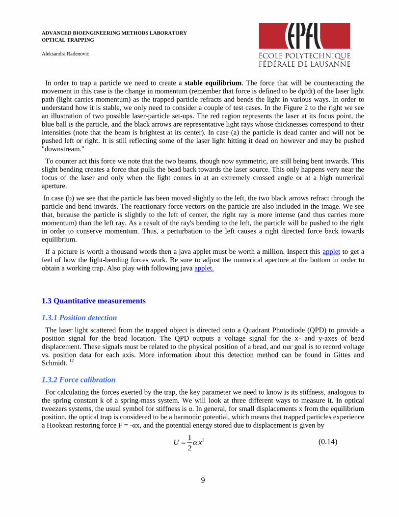
ADVANCED BIOENGINEERING METHODS LABORATORY
OPTICAL TRAPPING
Aleksandra Radenovic
18
Figure 7 GUI layout
2) When you run the GUI you will notice several different panels which will be used to control the stage and
perform the aforementioned calibrations and several axes whose purposes will be explained later The
GUI is initially launched with none of the piezo strain gauge or camera active-x controls displayed In
order to turn them on press the ldquoTurn Onrdquo push button in the upper left corner of the GUI in the ldquoPiezo
Controlsrdquo panel You will notice that 6 small piezo strain gauge and QPD active-x controls will be
initialized in the lower right of the GUI and the camera active-x control will be initialized in the middle
right of the GUI For the sake of this GUI you can ignore the piezo and strain gauge controls as they will
not be manually adjusted
3) The camera active-x control is initialized with the bdquoAutoGain‟ and bdquoAutoExposure‟ properties turned on
You will need to adjust these properties Most importantly Pixel clock should be set below 5M
4) Now adjust the objective slowly with the Z positioning knob until you can see floating beads in the Camera
window If you advance too far you will lift the slide off of the stage too little and you will not see the
beads
5) Refer to the laser operation section and following all safety procedures finally turn on the laser To turn it
you need to start the controllers first Make sure that you turn ON the TEMPERATURE controller first
(first red arrow left then red arrow right)
6) Now it is safe to turn ON also LASER DIODE controller (left green arrow) Don‟t change pre-set
parameters (20 000 kΩfor TSET) See Figure 8 They ensure proper functioning of laser diode Now turn on
the right green arrow and the laser diode should be on Yellow arrow Figure 8
ADVANCED BIOENGINEERING METHODS LABORATORY
OPTICAL TRAPPING
Aleksandra Radenovic
19
Figure 8 Laser diode controllers
7) Once you have turned up the power to the lasing power you will be able to see the laser reflected off of the
beads you trap or any glass you are focused on To find the edges of the cell first retract the objective in
the Z direction until you see the laser reflected in a bright circular pattern on the near coverslip To find the
far side advance the laser past the floating beads until you see the circular diffraction pattern on the
microscope slide The laser is in best focus just past the coverslip away from the microscope slide
8) This section discusses how to use the GUI to zero the strain gauges center the piezos and use the
nanometer precision positioning panel
- Zeroing the strain gauge cubes
Now you need to null the position reading on the strain gauge cubes In order to do this press the ldquoZerordquo push
button in the upper left corner of the GUI in the ldquoPiezo Controlsrdquo panel This button will set the x and y piezo
control outputs to 0V set the strain gauge position to 0V and then set both the x and y piezos in closed loop
(feedback) mode In addition it will move the piezos to the center of their output
- Centering the piezo cubes
This property of the GUI allows you to set all 3 piezo cubes (x y and z axes) to the middle of their output
range the approximate value of which is mentioned at the end of the previous section In addition it will zero
the output from the two DAQ analog output channels In order to execute this property press the ldquoResetrdquo push
button in the upper left corner of the GUI in the ldquoPiezo Controlsrdquo panel
- Nanometer accuracy 3-axis positioning
The three edit text boxes in the upper left corner of the GUI in the ldquoPiezo Controlsrdquo panel allow you to move
the stage by a specific displacement in nanometers In order to move the stage type the desired displacement in
nanometers in the edit text box corresponding to the cardinal axis upon which you would like to move Hit enter
in order to move the stage You can press enter multiple times to move the stage in increments of the entered
value This works for both positive and negative displacements If you exceed the range of the piezos which is
ADVANCED BIOENGINEERING METHODS LABORATORY
OPTICAL TRAPPING
Aleksandra Radenovic
20
set to be between 0 and 75V (this value should not be changed) you will no longer be able to move the stage
via this method In order to counteract this try to do the majority of the movement using the rough and fine
adjust knobs on the actual stage and use this property for final small displacements
9) The easiest way to trap a bead is to find one near the coverslip that is not stuck focus just past it and then
move the center of the trap over the bead It is highly recommended that at this time you mark the location
of the center of your trap on the computer screen Make an arrow-shaped piece of tape and use it to mark
the center of the bead on the screen This will make trapping much easier because you will have a rough
physical reference to the location of the laser
10) When the bead is trapped it will reflect the laser into the camera If the bead is not stuck to the glass you
should be able to move it in the X and Y directions and then very carefully advance the bead away from
the coverslip by advancing the objective by moving in the Z direction If the bead falls out of the trap try
again with another bead near the coverslip Trapping beads successfully away from the glass may take
some practice
11) Save an image of the trapped bead as shown on Figure 9
Figure 9 Trapped bead
26 Calibration
As is typical for instruments in AMBL the goal of this section is to relate the detector outputs to physical
quantities we would like to measure However before you proceed its important to consider laser power
dependence Both the position calibration as well as the stiffness of the trap depends greatly on the power
output of the 975nm trapping laser Therefore youll want to take data for 3-4 different trap power outputs in
the range of 30 60 and 90 mW (maximum power from laser diode is 90 mW at 260mA) and determine the
(hopefully linear) relationship between power and stiffness and power and QPD position readout Keep in
mind which of the measurements you make is dependent on accurate position calibration since youll need to
recalibrate when you change the laser power Observing specimens and trapping small objects is
straightforward with the procedures described above But to tap the full potential of the laser tweezers to
precisely quantify size position and forces at nm and pN scales requires careful calibration
To save time we are providing you with calibrations of the microscope image scale and the step-size of stage
movements by the picomotors We leave to you the more interesting calibrations including translating the
voltage measurements from the QPD into the position of the trapped particle relative to the center of the trap
(QPD position calibration) and the force exerted by the trap on the particle (trap stiffness calibration) There are
multiple techniques used to calibrate traps and well let you try a few of them and compare their results and
appropriateness Nevertheless please read the paragraph below about how to calibrate
ADVANCED BIOENGINEERING METHODS LABORATORY
OPTICAL TRAPPING
Aleksandra Radenovic
21
261 Voltage vs position calibration
What is Position Calibration To calibrate the position detection a relationship between the QPD output
voltages and position data must be determine Within a narrow range around the trap (about 100-200 nm) the
voltages Vx and Vy from the QPD are linearly related to the distance of the bead from the center of the trap
along each axis The position calibration also called sensitivity allows us to translate our raw Vx and Vy data
into distance data Sensitivity ρ is usually given in units of Voltsμm Of course the power setting of the laser
will affect the light intensity incident on the QPD and thus the voltage responses so rather than a single
conversion we really want the relationship between sensitivity and laser power This normally is fairly linear so
measuring sensitivity at 3 power levels is plenty to characterize the relationship
262 Stuck bead calibration (done by TA beforehand)
The calibration is performed by finding a 1μm bead attached to the glass surface (this sample is deliberately
mixed in a high-salt buffer to make the beads stick to the glass by hydrophobic interaction)
To make a slide with stuck beads use a ~1 M NaCl solution (provided) of 1300 dilution of 1 by weight 3μm
beads The best procedure to keep the beads from clumping is to first dilute the beads in a small amount of
distilled water (maybe 500μL) and then add the 50μL 1M NaCl solution For the stuck bead slide it is best to
let the slide rest for about 12 hour before using to let the beads settle onto the surface of the glass
Once the stuck bead slide is made load it and scan a stuck bead along the x- and y-axis while recording the
QPD signal A more precise method of calibration involves moving the bead in a grid pattern using either the
stage or a separate optical trap but our stage positioning does not have enough repeatability to enable this so
we will limit ourselves to measurements near the trap axes Estimated sensitivity is affected by focus This part
of the exercises has been performed by TA‟s before Typical sample position detection calibration curve for one
axis is shown in Figure 10
Remarks 90 mW of laser power at sample plane corresponds to asymp260 mA on current controller 60mW asymp175
mA and 30 asymp85 mA
Laser power [mW] Sensitivity α Vx ρ [Vnm] Sensitivityα Vy ρ [Vnm]
30 00061 00064
60 00042 00044
90 00035 00037
Figure 10 Sample position detection calibration curve for motion along a single axis
Position detector output [V] vs displacement [x] curve for a 097μm diam polystyrene
bead
Q8 How does sensitivity vary with power level Why this relation
minus2000 minus1000 0 1000 2000
minus4
minus3
minus2
minus1
0
1
2
3
4
Position (nm)
QP
DV
oltag
e(V
)
ADVANCED BIOENGINEERING METHODS LABORATORY
OPTICAL TRAPPING
Aleksandra Radenovic
22
27 Measurement of the trap stiffness
271 Power Spectrum Method
The thermal motion of a spherical bead of known size suspended in water is well characterized As the laser
power is turned up on a trapped bead the Brownian motion of the bead is constrained more and more by the
increasing trap force restoring the bead to the center of the trap A statistical analysis of this motion allows us to
estimate both the sensitivity of the trap and its stiffness
The PSD Method stiffness measurement requires knowledge of the hydrodynamic drag on the particle For a
sphere the Stokes drag relation is well known and requires knowing the diameter of the bead and viscosity of
the fluid The Stokes relationship is not valid close to a wall so a particle must not be near the surface of a slide
or coverslip
The OTkb program puts in the table the calculated trap stiffness by fitting your PSD data to Lorenzian Now
we explain what how program derives the trap stiffness from the PSD data The Power Spectral Density (PSD)
of a trapped bead has a Lorentzian profile described by
2
2 2 2
0( )
Bvv
k TS
f f
(015)
in V2Hz Where β = 3πηd is the drag η is the fluid viscosity of water d is the diameter of the bead ρ is the
sensitivity of the trap and f is the frequency of bead vibrations If the fluid is water then we can take η = 890
10 - 4
Pa s Using this a curve can be fit to the log of the data sets giving the rolloff frequency fo In addition
the rolloff frequency relates to the relaxation time
0
0
1
2 f
(016)
One useful analytic method for this part of the lab minimizes the least-squares distance of every point from the
predicted curve giving two parameters of the equation alpha and fo The Lorentzian can be recast as the
equation
2 2
0log ( ) log log( )vvS f f f (017)
The rolloff frequency parameters found through fitting gives the trap stiffnesses κ from the following relation
κ= 2πfoβ again where β = 3πηd is the drag η = 890 10 - 4
Pa s is the viscosity of water and d is the diameter
of the bead (in meters) This is enough information to calculate and output trap stiffnesses
272 Stokes drag
A second method of calculating the traps stiffness is by calculating the drag force F=αx exerted on a bead as
the stage is moved The most basic formulation of the force exerted on a sphere by fluid flowing past it is
3x v dv (018)
ADVANCED BIOENGINEERING METHODS LABORATORY
OPTICAL TRAPPING
Aleksandra Radenovic
23
Where v is the flow velocity η = 890 10 - 4
Pa s is -the viscosity of water and d is the diameter of the bead
(in meters) Note that this equation only applies for constant velocity The Stokes subprogram will run the bead
back and forth at various stage velocities its therefore important that the stage micrometers have ample
movement left and that there are few other beads in the area far from trapped bead 7
Most theory about microspheres in traps involves the Stokes drag formula However when a bead is close to a
surface the formula doesn‟t hold anymore and we need to use something called Faxenrsquos law Stokes equation
then needs to be corrected due to the proximity effects by factor g that can be approximated by Faxen‟s law
13 4 5
9 1 45 11
16 8 256 16
r r r rg
h h h h
(019)
Where h is a distance from the coverslip and r is bead radius This equation is valid for h-rge002r The factor g
takes values between 1 and 3
273 Data acquisition
Please record in your notebook the values generated by both methods for the three different laser powers and
enter corresponding sensitiveness given in table 1 To do so
1) Starting with a slide loaded with a sparse suspension of beads in water trap a bead and move it well away
from the coverslip slide and from other beads (If you have centered the QPD at the highest power setting
you wont have to release the bead and recenter between power settings)
2) Before taking data align the signal on QPD by pressing QPD alignment start once the signal is centered on
QPD
3) Enter the correct value for bead diameter
4) Specify the filename and directory to save your data (You need to change a file name EACH TIME YOU
CHANGE CONDITIONS laser power or axis for example PSD30mWx or STOKES60mWy etc)
5) Now press PSD Start Default sampling frequency is 100 000 Hz (but it can be changed if changed note it
in your logbook) Default sampling time is 3 seconds You can change axis by pressing Current axis
button Once done software will display the PSD as a function of the frequency image as shown below on
Fig 11
Figure 11 Power spectrum of V[t] for a 097μm beads
in water solution at room temperature Laser power is 90 m
ADVANCED BIOENGINEERING METHODS LABORATORY
OPTICAL TRAPPING
Aleksandra Radenovic
24
6) Then Run the Stokes watch the movement on the video capture If additional beads fall into the trap
discard the data If this is a consistent problem ask for help from a TA - a more dilute bead solution may
need to be made Make sure to run the Stokes program for both the x- and y-axes and all there laser power
as for PSD the program calculates the trap stiffness
7) Repeat data collection for both methods at each of the laser power settings you have chosen for your
calibration
3 DATA ANALYSIS
1) There is some experimental data available for a 1μm trapped microsphere on the course server (filename
trapdatatxt size ca 5Mb) This is a time-series of position data along one dimension for a microsphere
The data is collected at 200 kSs so the time-interval between each point is 5μs The units are in some
esoteric unit preferred by the experimenter (raw output of a 16-bit AD-conversion)
Download the data import it into MATLAB or some other data-analysis program of your choice
You can remove the average of the data from all data points to center it around zero
Calculate and plot the power spectral density in a log-log figure (in matlab this can be done with the
pwelch function)
Fit your result derived in excel to the data and determine the roll-off frequency You will need two
fitting parameters an overall constant that scales the curve and the roll-off frequency In matlab you
can use the function lsqcurvefit to do the fitting
Q9 What is the roll-off frequency What is the stiffness of the trap
2) Plot the trap stiffness for both axis as a function of laser power
3) Compare the results obtained using PSD and Stokes drag method Do you remark some differences Why
4) Think or speculate about why Stokes formula doesn‟t work near a wall (Hint find a hydrodynamics book
where Stokes law is derived and think about the assumptions Search the library or the web and find out
one formula (there are probably many) for Faxens law (it should look like Stokes law but involve the
distance to the wall somehow)
Q10 Your friend is doing an experiment with a 2μm microsphere which is trapped so that the center of the
sphere is 5μm above a glass coverslip How large is the error (in percent) heshe is making when using
Stokes law
5) Plot and fit PSDs for the data you took during the 1st session using the procedure you developed in 1)
Q11 Compute a histogram for the trapdata data set of the time-series and use the stiffness you calculated
What is the position sensitivity of the detector that has been used
ADVANCED BIOENGINEERING METHODS LABORATORY
OPTICAL TRAPPING
Aleksandra Radenovic
25
4 REFERENCES
1 Lebedev P N Experimental Examination of Light Pressure Annalen der Physik 6 433-458 (1901)
2 Ashkin A Acceleration and trapping of particles by radiation pressure Physical Review Letters 24 156-159 (1970)
3 Ashkin A Applications of Laser-Radiation Pressure Science 210 1081-1088 (1980)
4 Ashkin A Forces of a Single-Beam Gradient Laser Trap on a Dielectric Sphere in the Ray Optics Regime Biophysical Journal 61
569-582 (1992)
5 Ashkin A amp Dziedzic J M Optical Trapping and Manipulation of Viruses and Bacteria Science 235 1517-1520 (1987)
6 Cox A J DeWeerd A J amp Linden J An experiment to measure Mie and Rayleigh total scattering cross sections American
Journal of Physics 70 620-625 doiDoi 10111911466815 (2002)
7 Smith S B Cui Y J amp Bustamante C Optical-trap force transducer that operates by direct measurement of light momentum
Biophotonics Pt B 361 134-162 (2003)
8 Conroy R S et al Optical waveguiding in suspensions of dielectric particles Applied Optics 44 7853-7857 (2005)
9 Svoboda K amp Block S M Optical Trapping of Metallic Rayleigh Particles Optics Letters 19 930-932 (1994)
10 Stamper-Kurn D M et al Optical confinement of a Bose-Einstein condensate Physical Review Letters 80 2027-2030 (1998)
11 Nieminen T A Rubinsztein-Dunlop H amp Heckenberg N R Calculation and optical measurement of laser trapping forces on
non-spherical particles J Quant Spectrosc Ra 70 627-637 (2001)
12 Gittes F amp Schmidt C F Interference model for back-focal-plane displacement detection in optical tweezers Optics Letters 23 7-
9 (1998)
Additional literature
1 MITs Optical Trapping Experiment a sister lab to our own
J Bechhoefer S Wilson Faster cheaper safer optical tweezers for the undergraduate laboratory Am J Phys 70 (4) Apr 2002 Read
Optical tweezer theory and Applications part B and Appendix for Trapped-Particle Statistical Analysis explanation
2 Optical Tweezers from Wikipedia
3 J W Shaevitz A Practical Guide to Optical Trapping a less technical description of the optical set up and detection
(Not everything here is relevant to us but it serves as an excellent starter guide)
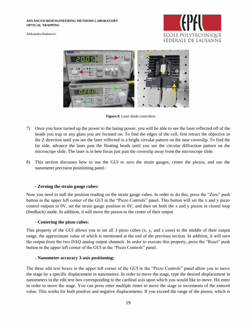
ADVANCED BIOENGINEERING METHODS LABORATORY
OPTICAL TRAPPING
Aleksandra Radenovic
25
4 REFERENCES
1 Lebedev P N Experimental Examination of Light Pressure Annalen der Physik 6 433-458 (1901)
2 Ashkin A Acceleration and trapping of particles by radiation pressure Physical Review Letters 24 156-159 (1970)
3 Ashkin A Applications of Laser-Radiation Pressure Science 210 1081-1088 (1980)
4 Ashkin A Forces of a Single-Beam Gradient Laser Trap on a Dielectric Sphere in the Ray Optics Regime Biophysical Journal 61
569-582 (1992)
5 Ashkin A amp Dziedzic J M Optical Trapping and Manipulation of Viruses and Bacteria Science 235 1517-1520 (1987)
6 Cox A J DeWeerd A J amp Linden J An experiment to measure Mie and Rayleigh total scattering cross sections American
Journal of Physics 70 620-625 doiDoi 10111911466815 (2002)
7 Smith S B Cui Y J amp Bustamante C Optical-trap force transducer that operates by direct measurement of light momentum
Biophotonics Pt B 361 134-162 (2003)
8 Conroy R S et al Optical waveguiding in suspensions of dielectric particles Applied Optics 44 7853-7857 (2005)
9 Svoboda K amp Block S M Optical Trapping of Metallic Rayleigh Particles Optics Letters 19 930-932 (1994)
10 Stamper-Kurn D M et al Optical confinement of a Bose-Einstein condensate Physical Review Letters 80 2027-2030 (1998)
11 Nieminen T A Rubinsztein-Dunlop H amp Heckenberg N R Calculation and optical measurement of laser trapping forces on
non-spherical particles J Quant Spectrosc Ra 70 627-637 (2001)
12 Gittes F amp Schmidt C F Interference model for back-focal-plane displacement detection in optical tweezers Optics Letters 23 7-
9 (1998)
Additional literature
1 MITs Optical Trapping Experiment a sister lab to our own
J Bechhoefer S Wilson Faster cheaper safer optical tweezers for the undergraduate laboratory Am J Phys 70 (4) Apr 2002 Read
Optical tweezer theory and Applications part B and Appendix for Trapped-Particle Statistical Analysis explanation
2 Optical Tweezers from Wikipedia
3 J W Shaevitz A Practical Guide to Optical Trapping a less technical description of the optical set up and detection
(Not everything here is relevant to us but it serves as an excellent starter guide)