TUGAS PROPULSI KAPAL LANJUT

A Numerical Study of The Propulsive Efficiency of aFlapping Hydrofoil

DISUSUN OLEH :Muhammad Habib Chusnul Fikri ( 4211 100 043)

JURUSAN TEKNIK SISTEM PERKAPALANFAKULTAS TEKNOLOGI KELAUTAN

INSTITUT TEKNOLOGI SEPULUH NOPEMBER SURABAYA

A numerical study of the propulsive e�ciencyof a �apping hydrofoil

SUMMARY

KEY WORDS: �apping hydrofoil; swimming propulsion; hydrofoil e�ciency

1. INTRODUCTION

In aerodynamics and hydrodynamics, bird �ight and �sh swimming have inspired and guidedthe development of aircraft and underwater vehicles. It is interesting, however, to note howprimitive these man-made machines seem compared to their natural counterparts in terms ofintelligence, e�ciency, agility, adaptiveness and functional complexity. These and other similarobservations and issues have been addressed by the scienti�c community, have triggered theformulation of the science of biomimetics and have inspired new approaches to old problems.Problems in the self-propulsion of deformable bodies through �uids invite the co-operation oftools from structural mechanics, theoretical and experimental hydrodynamics, computational�uid dynamics and control theory, to name a few.

1.1. Background and motivation

The highly e�cient swimming mechanisms of some �sh can potentially provide inspirationfor design of propulsive systems that will outperform the thrusters and propellers currently in

A computational �uid dynamics study of the swimming e�ciency of a two-dimensional �apping hydro-foil at a Reynolds number of 1100 is presented. The model accounts fully for viscous e�ects that areparticularly important when �ow separation occurs. The model uses an arbitrary Lagrangian–Eulerian(ALE) method to track the moving boundaries of oscillatory and �apping bodies. A parametric analysisis presented of the variables that a�ect the motion of the hydrofoil as it moves through the �ow alongwith �ow visualizations in an attempt to quantify and qualify the e�ect that these variables have on theperformance of the hydrofoil.

use. The advantages of noiseless propulsion associated with a less conspicuous wake couldbe particularly useful for military applications. Thus, there is a need to further our knowl-edge of the hydrodynamics and �uid–structure interactions in �sh swimming and to providebenchmarks for new theoretical developments and designs. Propulsion by means of oscillatinghydrofoils has been the focus of considerable interest in recent years. Applications that couldsubstantially bene�t from this technology include autonomous underwater vehicles.The �apping hydrofoil is the primary component in �sh propulsion kinematics. The objective

of this paper is to understand the hydrodynamics and �uid–structure interactions in pitchingand heaving hydrofoils. In particular, the present work attempts to further our understandingof the mechanisms which a�ect thrust and e�ciency by modelling the wake structure and itsevolution. This research e�ort involves the development of computational methods and toolsto simulate the �uid–structure interaction dynamics of a �apping hydrofoil, and the results arecompared with benchmark experimental case studies reported in the literature. Furthermore,the present work represents a small but important step in a broad research program in the areaof design of adaptive undersea vehicles that generate thrust using vorticity control mechanisms(i.e. �apping foil combined with body deformation).

1.2. Propulsion studies

Many researchers have addressed the problem of foil motion in the context of aerodynamicand hydrodynamic propulsion. In particular, the �apping foil propulsion, similar to the thun-niform mode of propulsion, has received considerable attention in recent years. In thunniformpropulsion, the caudal �n acts a the main propulsive element, providing up to 90% of thethrust. Researchers have attempted to formulate mathematical models to further understand theobserved kinematics of �sh. The �apping hydrofoil produces thrust as it oscillates developinga reverse K�arm�an vortex street (which has vortices rotating in opposite directions to the classi-cal K�arm�an vortex street) that corresponds to a jet-like average velocity pro�le. However, suchjets are convectively unstable and there is only a narrow bandwidth of frequencies for whichthe K�arm�an vortices and the jet-like pro�le co-exist and the �ow is stable as demonstrated byTriantafyllou et al. [1]. Early hydrodynamic models were based on a quasi-static approach thatuses steady-state �ow theory to calculate the �uid forces for sequential frames of the motion.These models were restricted to simple body shapes and forms. Later models have dealt withmore realistic assumptions. Lighthill [2] applied the slender body theory of hydrodynamics totransverse oscillatory motions of slender �sh. This study revealed the high propulsive e�ciencyof �sh, a �nding that alone renders the utilization of similar propulsive techniques in man-madevehicles a very attractive quest. Other studies included analyses of a slender wing with passivechordwise �exibility [3], two-dimensional potential �ow modelling over a thin waving plate of�nite chord by Wu [4] and Siekmann [5], and a planar modelling of �ow over a waving plateof �nite thickness by Uldrick and Siekmann [6]. Wu not only studied the hydromechanics ofswimming propulsion [7], he also researched optimum shape problems [8] and the hydrome-chanics of slender �sh with side �ns. Three-dimensional models have more recently beendeveloped by Cheng et al. [9] and Bandyopadhyay et al. [10] who have utilized waving platetheory as well as comparisons of performance coe�cients between �sh and underwater vehicles.Other researchers such as Isshiki and Murakami [11], Koochesfahani [12], Triantafyllou

et al. [13] and Gopalkrishnan et al. [14] have addressed the problem of the thrust-producingcapability of moving hydrofoils. Ramamurti et al. [15] studied �apping airfoils using an

incompressible �ow solver. Tuncer and Platzer [16] also conducted a computational study of�apping airfoil dynamics.In terms of experimental work, Anderson’s PhD thesis [17] on vorticity control provides

excellent data with which to compare results. The experimental work concentrated on the�ow around pitching and heaving airfoils at a Reynolds number of 1100. Koochesfahani [18]also studied experimentally a pitching airfoil at a Reynolds number of 12 000. Robotuna [18],a robotic undersea vehicle, designed and constructed at the Massachusetts Institute of Tech-nology (MIT) has demonstrated that thunniform propulsion is indeed very e�cient. Robotunaachieved e�ciencies on the order of 91%, not including losses in the actuators.In this body of work, a computational �uid dynamics research code (CFDLIB, [19]) based

on structured grids is used to study the unsteady �ow past oscillating hydrofoils at lowReynolds numbers. The viscous �ow past a NACA0012 hydrofoil at various pitching andheaving frequencies and other design parameters is simulated. The variation of the force coef-�cient with reduced frequency is compared to the experimental work published by Anderson.In all the numerical studies cited, it has been observed that the published data has failedto appropriately quantify the e�ciency of the thrust producing hydrofoil. The present paperattempts to address this issue and presents a quantitative analysis on the e�ciency of the�apping hydrofoil used in the thunniform mode of propulsion as a function of the Strouhalnumber which depends on the vortex shedding frequency and wake width.

1.3. Flow over static and oscillating cylinders

The unsteady viscous �ow behind a circular cylinder has been the object of numerous exper-imental and numerical studies, especially from the �uid mechanics point of view, because ofthe fundamental mechanisms that this �ow exhibits. A case that is often used to benchmarkcodes and that has been studied extensively is the oscillating cylinder.Blackburn and Henderson [20] studied the �ow past an oscillating cylinder utilizing a spec-

tral method. They limited the oscillation amplitude to one case and studied the �ow when thecylinder is oscillated at a frequency close to its shedding frequency. Mendes and Branco [21]applied their �nite element code to a cylinder in cross-�ow oscillation with a lower ampli-tude of motion as well as at a lower Reynolds number of 200. Koopman [22] conductedan experimental study of the wake geometry behind oscillating cylinders at low Reynoldsnumbers (100, 200 and 300). Tanida et al. [23] also conducted experimental research on thestability of circular cylinders in uniform �ow or in the wake of another cylinder. Mittal andTezduyar [24–26] developed a �nite element code and studied various incompressible �owcases including oscillating cylinders and airfoils.In this paper, the oscillating cylinder is used as a benchmark to validate the CFD code used.

This benchmark tests the capacity of the CFD code to not only properly resolve unsteady �owsas well as �ows where there is boundary movement.

2. FLUID FLOW MODELLING

Unsteady viscous �ow is governed by the continuity and Navier–Stokes equations:

∇ · (�u) = 0 (1)

@�u@t+∇ · (�uu) =−∇p+∇ ·�+ �F (2)

The above equations express conservation of mass and momentum, respectively, and accountfor the spatial and temporal distributions of the velocity vector, u, and the pressure �eld p.For an incompressible �ow �eld, the density � is constant spatially and in time. � is thedeviatoric stress tensor in which are prescribed viscous stresses, turbulent stresses or elastic–plastic material deformation. F de�nes the body forces present.A �nite-volume discretization technique is used to reduce the set of di�erential equations

given by Equations (1) and (2) into a system of algebraic equations corresponding to thenodes of the computational mesh.To account for mesh movement, an arbitrary Lagrangian–Eulerian (ALE) formulation is

used. In a Lagrangian formulation, the mesh moves such that the control volumes coincide withmaterial volumes and there is no advection relative to it. In a purely Eulerian method, the meshdoes not move and there is advection relative to it. The ALE method (see Reference [27])combines these two, to allow for mesh movement, and not necessarily with the �uid �ow. Todo this, the hydrodynamic time-step is split into a Lagrangian phase and a rezone–remap phase.In the Lagrangian phase, the �uid dynamics is taken into account and the mesh moves withthe �uid to a new position. In rezoning, a new mesh is de�ned and remapping is performed totransfer the state variables to this new mesh. The details of the ALE methodology are givenin References [19, 27], and only an overview of the salient aspects of the numerical methodare given here.For the purpose of discretization, it is convenient to recast Equations (1) and (2) in their

control volume formulation, namely:

∫Sa(t)

�(u − ua)n dS =0 (3)

ddt

∫Va(t)�u dV +

∫Sa(t)

�u(u − ua)n dS =−∫Sa(t)

pn dS +∫Sa(t)

n�dS +∫Va(t)

�F dV (4)

This formulation accounts for an arbitrary moving control volume. Sa(t) is the surface ofthe control volume Va(t). The outward unit normal to the surfaces is n. The movement ofthe control volume is de�ned by ua = dxa=dt. In the use of these equations, conservationof volume is maintained:

dVa(t)dt

=∫Sa(t)

uan dS (5)

Following the de�nition of Eulerian and Lagrangian formulations, one can expect that fora purely Lagrangian formulation ua = u and for a purely Eulerian formulation ua = 0.Equations (3) and (4) are cast in a conservative form, and are a combination of the �uid

dynamics (the Lagrangian phase) and the mesh movement (remapping). In the Lagrangianphase, one sets the volume velocity to be equal to the �uid velocity, i.e. ua = u. Equation (4)becomes:

ddt

∫VL�u dV = −

∫SLpn dS +

∫SLn�dS +

∫VL�F dV (6)

where VL is the Lagrangian control volume and SL its surface. The time derivatives refer to thisvolume. The distorted mesh obtained in the Lagrangian phase can be altered by remapping:

ddt

∫Sk

�uRn dS =0 (7)

ddt

∫Vk

�u dV −∫Sk

�uuRn dS =0 (8)

where uR = ua−u and is the mesh velocity relative to the Lagrangian frame. Vk is the controlvolume de�ned by the mesh velocity ua with Sk being its surface. This control volumechanges the mesh from its initial value VL to its �nal one V ∗

k . This method is known asintegral remapping.The �ow solver used is CFDLIB, which uses a cell-centred, �nite volume method with

explicit time-stepping. The �ow �eld is discretized using a central di�erencing method.

3. PERFORMANCE PARAMETERS

In the study of both the oscillating cylinder and �apping hydrofoil, several parameters areused to quantify the �ow characteristics. In this section, these parameters are presented.With both the cylinder and hydrofoil, drag and lift coe�cients provide important data

essential to this study:

CD =D

12 �U

2lb(9)

CL =L

12 �U

2lb(10)

where b is the span of the hydrofoil or cylinder which is set to 1 and l is a characteristiclength. In the case of the cylinder, its diameter is used (l=d) while in the case of the hydrofoilthe chord length is used (l= c). In both cases, the total lift and drag can be divided intoits pressure (force due to pressure �eld) and viscous (force due to shear stress) components.This is done throughout the paper.Since the hydrofoil’s main task is to produce thrust, it is often more convenient to think

in terms of thrust instead of drag. Thrust is equal but opposite in direction to the drag force,therefore one has

CT = − CD = T12 �U

2cb(11)

The average thrust is de�ned as

〈T 〉= 1�

∫ �

0T dt (12)

where � is the signal period. As in the case of the waving plate, power can be de�ned as theamount of energy imparted to the airfoil for it to overcome the �uid forces:

P(t)= − L(t) dhdt

−M (t) d�dt

(13)

where M (t) is the moment created by the lift and drag forces at the pitching axis and isnon-dimensionalized by

CM =M

12 �U

2c2b(14)

The sign on both terms (in Equation (13)) is negative as the lift force and moment are reactionforces created by the �uid as the airfoil moves through it. Power can also be averaged overtime:

〈P〉= 1�

∫ �

0P dt (15)

and also non-dimensionalized:

CP=P

12 �U

3cb(16)

E�ciency is a measure of the energy lost in the wake versus energy used in creating thenecessary thrust:

�=〈T 〉U〈P〉 (17)

The frequency and heave amplitude can be non-dimensionalized by using the followingparameters. The �rst is the wave number k:

k=!c2U

=�fcU

(18)

with a more indicative parameter being the Strouhal number which is based not only on theshedding frequency but also on the wake width. Since the wake width is di�cult to determine,one can approximate it with the amplitude of motion of the hydrofoil:

Sth=2h0fU

(19)

In the case of the oscillating cylinder, the wake width is also approximated by the amplitudeof motion.

4. OSCILLATING CYLINDER IN UNIFORM FLOW

The code was validated using a cylinder in a uniform �ow with cross-�ow oscillation. This isa well-studied phenomenon and the combination of moving boundary and vortex shedding isvery similar to the dynamics observed with �apping hydrofoils. In this section, a comparison

h

x

y

U

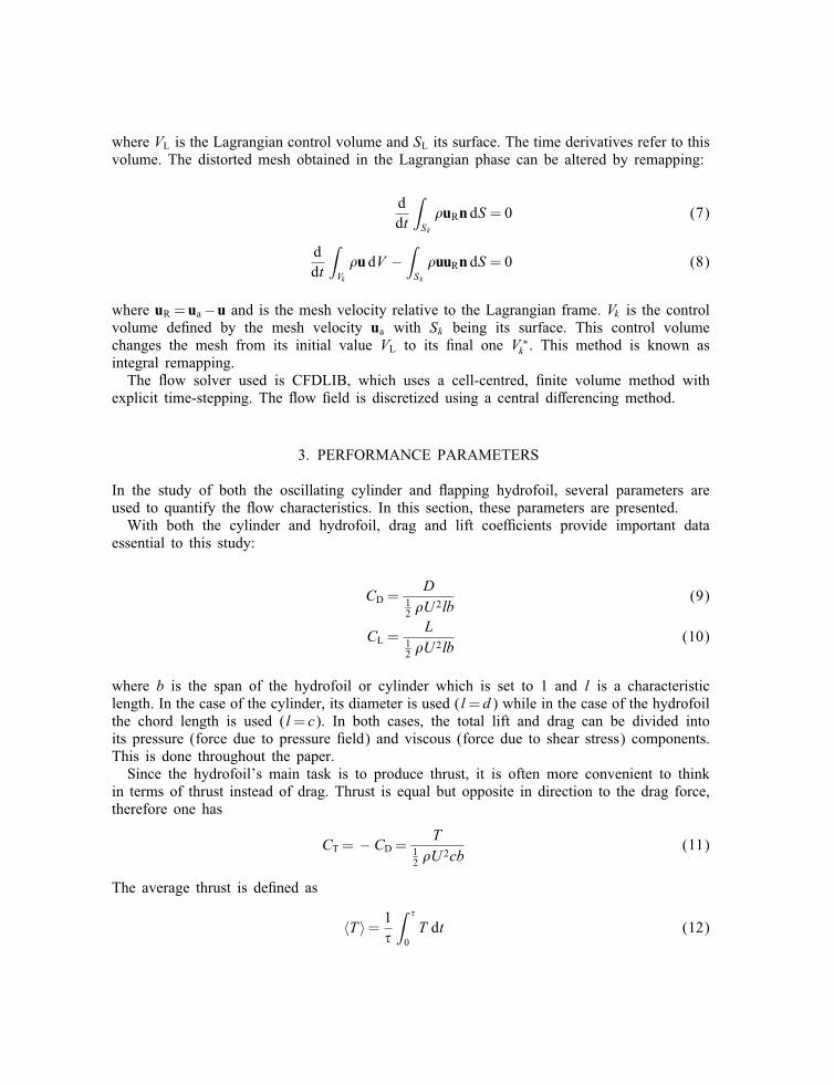
Figure 1. Problem de�nition of an oscillating cylinder in uniform �ow.The distance from the centreline is h.

of the results obtained using CFDLIB with ones obtained in the literature will be made. Inparticular, the comparison will be made with results obtained by Blackburn and Henderson[20]. This paper was chosen due to the Reynolds number (500) that was used, which is pastthe transitional Reynolds number of 400 after which the energy transfer phase switch canoccur. Also, the authors used a spectral method to solve the �ow �eld. These methods tendto be particularly accurate.The problem consists of a cylinder of diameter d oscillating in a direction perpendicular (y)

to the uniform velocity �eld direction (x). The study, as in the literature, was performedat a Reynolds number (Ud=�) of 500. One of the most interesting aspects of this kind ofoscillation is called the lock-in phenomena. During lock-in, the vortex shedding frequencyis the same as the oscillation frequency of the cylinder, therefore, the oscillation drives thevortex shedding. This occurs at oscillation frequencies approximately equal to the sheddingfrequency of the static cylinder. Simulations were performed with a static cylinder and theStrouhal number was measured to be equal to 0.21.The relative frequency is de�ned as

F =f0fv

(20)

where f0 is the oscillating frequency and fv is the vortex shedding frequency in the staticcase. The motion of the cylinder is governed by

h(t)= hmax sin(2�f0(t − tstart)) (21)

where hmax is the maximum displacement from the centreline and tstart is when the oscillationbegins (Figure 1).Lock-in occurs at an interval of F close to 1. For lower amplitudes of oscillation, this

interval diminishes. Koopman [22] reported that entrainment (lock-in) can only occur forhmax=d¿0:05. Therefore, entrainment is assured for a value of hmax =0:25d. Another inter-esting phenomenon is the phase reversal that occurs between F =0:90 and 0.98. The phases

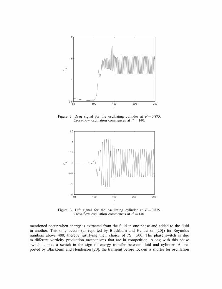
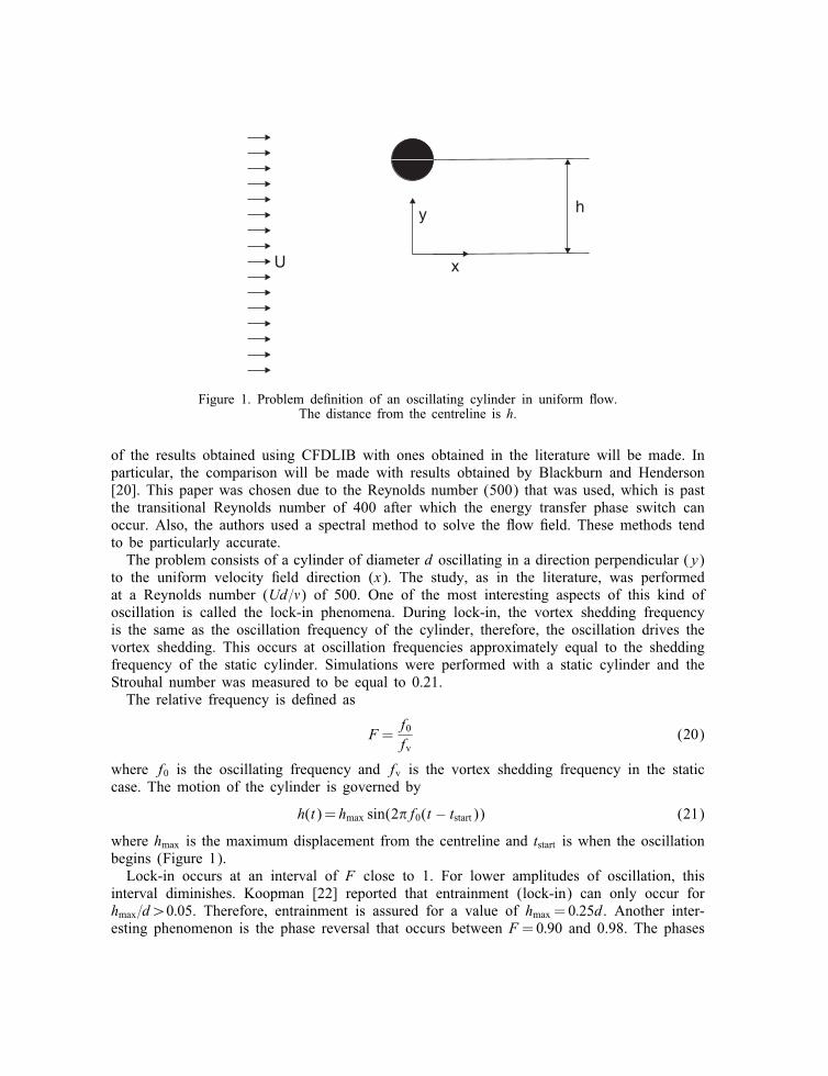
Figure 2. Drag signal for the oscillating cylinder at F =0:875.Cross-�ow oscillation commences at t∗=140.

Figure 3. Lift signal for the oscillating cylinder at F =0:875.Cross-�ow oscillation commences at t∗=140.

mentioned occur when energy is extracted from the �uid in one phase and added to the �uidin another. This only occurs (as reported by Blackburn and Henderson [20]) for Reynoldsnumbers above 400; thereby justifying their choice of Re=500. The phase switch is dueto di�erent vorticity production mechanisms that are in competition. Along with this phaseswitch, comes a switch in the sign of energy transfer between �uid and cylinder. As re-ported by Blackburn and Henderson [20], the transient before lock-in is shorter for oscillation

Table I. Comparison of results with ones obtained by Blackburn and Henderson [20].

Literature Present study

F 〈Cd〉 max |Cl| 〈Cd〉 max |Cl|0.875 1.46 0.72 1.35 0.67

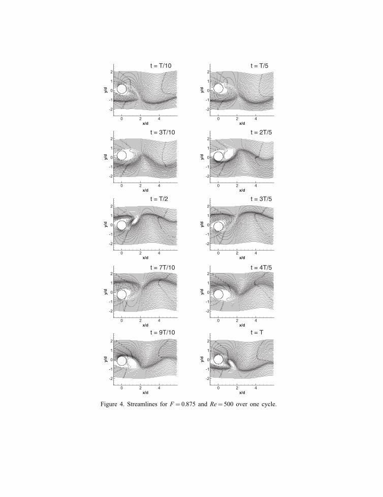
frequencies slightly below the vortex shedding frequency. Therefore, the simulations were runat F =0:875. The drag and lift curves are plotted in Figures 2 and 3. The cylinder was forcedto begin oscillating at a non-dimensional time (t∗= tU=d) equal to 140. Both the averagedrag and maximum lift (see Table I) compare favourably with results obtained by Blackburnand Henderson [20]. The streamlines over one cycle are plotted in Figure 4 and shows theformation of the vortices along with the areas of higher �uid velocity which are denoted bythe higher density of streamlines.As can be seen from Figures 2 and 3 the cylinder is kept static until the vortex shedding

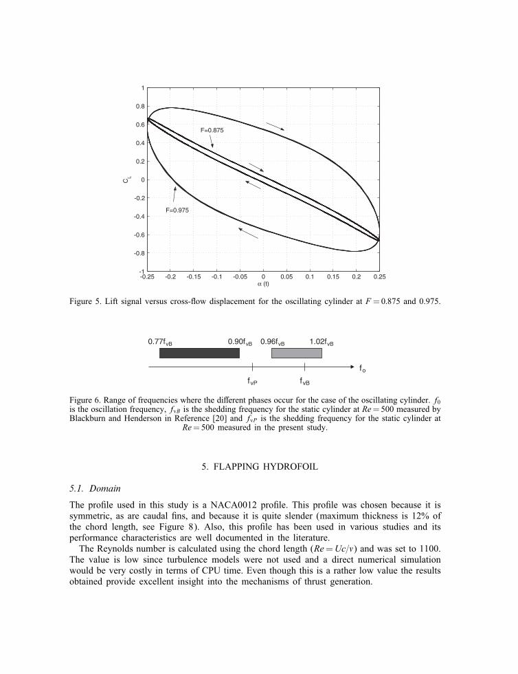
is stable and is then oscillated. The transient time is relatively short, approximately 30 timeunits. Also, the lift coe�cient is plotted against the cross-�ow coe�cient in Figure 5.This plot compares very favourably with the one in Reference [20] for the case F =0:875

and less favourably for F =0:975. This is due to the fact that the phase switch has notyet occurred. The fact that the phase switch has not occurred contradicts Blackburn andHenderson’s claims. The di�erence is that in the present study, the Strouhal number calculatedfor the static cylinder is too low. Figure 6 highlights the problem. The light grey area denotesthe phase where the cylinder transfers energy to the �uid (between F =0:98 and 1.02) whilethe black area denotes the phase where energy is extracted from the �uid (F =0:77–0.90).The frequencies fvB and fvP are the vortex shedding frequencies calculated for the staticcylinder in Reference [20] and in the present study, respectively. As can be clearly seen theshedding frequency calculated in the present study has a smaller value than the one calculatedby Blackburn and Henderson. The results obtained in the present study show that in fact, theStrouhal number calculated by Blackburn and Henderson is a better �t in relation to thelocation of the phases present.Since the range of frequencies over which the �uid to cylinder energy transfer occurs is

quite large in relation to the other phase, it is much easier to obtain favourable simulationresults in that range. The other phase presents a greater challenge, as it exists over a smallrange. This is why the results obtained for F =0:875 are very similar in relation to the resultsobtained by Blackburn. In the F =0:975, the shedding regime is transitional and thereforea degraded hysteresis curve is developed (Figure 5). In an attempt to reproduce the lock-in atapproximately F =1, obtained by Blackburn and Henderson, a simulation was performed at anon-dimensional frequency of 1.05. This would place the Strouhal number at approximately thevalue obtained by Blackburn and Henderson. The lock-in is never achieved and a quasi-chaotictransient is never surpassed. This transient is very similar to the one obtained by Blackburnand Henderson, with the di�erence that they achieved a lock-in after approximately 1200 timeunits.These results validate the CFD code used and allow for the simulation of more complex

geometries, i.e. the �apping hydrofoil.

t = T/10 t = T/5

t = 3T/10 t = 2T/5

t = T/2 t = 3T/5

t = 7T/10 t = 4T/5

t = 9T/10 t = T

Figure 4. Streamlines for F =0:875 and Re=500 over one cycle.

-0.25 -0.2 -0.15 -0.1 -0.05 0 0.05 0.1 0.15 0.2 0.25-1

-0.8

-0.6

-0.4

-0.2

0

0.2

0.4

0.6

0.8

1

α (t)

CL

F=0.875

F=0.975

Figure 5. Lift signal versus cross-�ow displacement for the oscillating cylinder at F =0:875 and 0.975.

fo

fvBfvP

0.96fvB 1.02fvB0.90fvB0.77fvB

Figure 6. Range of frequencies where the di�erent phases occur for the case of the oscillating cylinder. f0is the oscillation frequency, fvB is the shedding frequency for the static cylinder at Re=500 measured byBlackburn and Henderson in Reference [20] and fvP is the shedding frequency for the static cylinder at

Re=500 measured in the present study.

5. FLAPPING HYDROFOIL

5.1. Domain

The pro�le used in this study is a NACA0012 pro�le. This pro�le was chosen because it issymmetric, as are caudal �ns, and because it is quite slender (maximum thickness is 12% ofthe chord length, see Figure 8). Also, this pro�le has been used in various studies and itsperformance characteristics are well documented in the literature.The Reynolds number is calculated using the chord length (Re=Uc=�) and was set to 1100.

The value is low since turbulence models were not used and a direct numerical simulationwould be very costly in terms of CPU time. Even though this is a rather low value the resultsobtained provide excellent insight into the mechanisms of thrust generation.

ha

ld

Block 1

Block 2

Block 3

ji

jij

i

U

Inflo

wbo

unda

ry

Symmetry

Symmetry

Zero gradient

outflow boundary

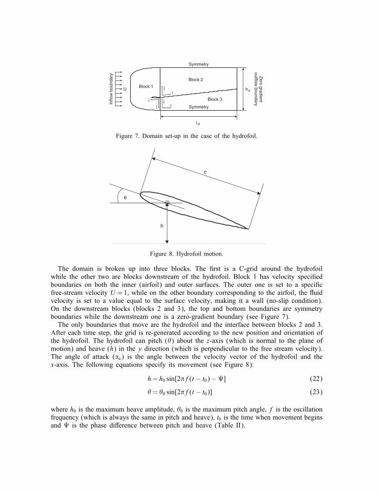
Figure 7. Domain set-up in the case of the hydrofoil.

θ

c

h

Figure 8. Hydrofoil motion.

The domain is broken up into three blocks. The �rst is a C-grid around the hydrofoilwhile the other two are blocks downstream of the hydrofoil. Block 1 has velocity speci�edboundaries on both the inner (airfoil) and outer surfaces. The outer one is set to a speci�cfree-stream velocity U =1, while on the other boundary corresponding to the airfoil, the �uidvelocity is set to a value equal to the surface velocity, making it a wall (no-slip condition).On the downstream blocks (blocks 2 and 3), the top and bottom boundaries are symmetryboundaries while the downstream one is a zero-gradient boundary (see Figure 7).The only boundaries that move are the hydrofoil and the interface between blocks 2 and 3.

After each time step, the grid is re-generated according to the new position and orientation ofthe hydrofoil. The hydrofoil can pitch (�) about the z-axis (which is normal to the plane ofmotion) and heave (h) in the y direction (which is perpendicular to the free stream velocity).The angle of attack (�a) is the angle between the velocity vector of the hydrofoil and thex-axis. The following equations specify its movement (see Figure 8):

h= h0 sin[2�f(t − t0)−�] (22)

�= �0 sin[2�f(t − t0)] (23)

where h0 is the maximum heave amplitude, �0 is the maximum pitch angle, f is the oscillationfrequency (which is always the same in pitch and heave), t0 is the time when movement beginsand � is the phase di�erence between pitch and heave (Table II).

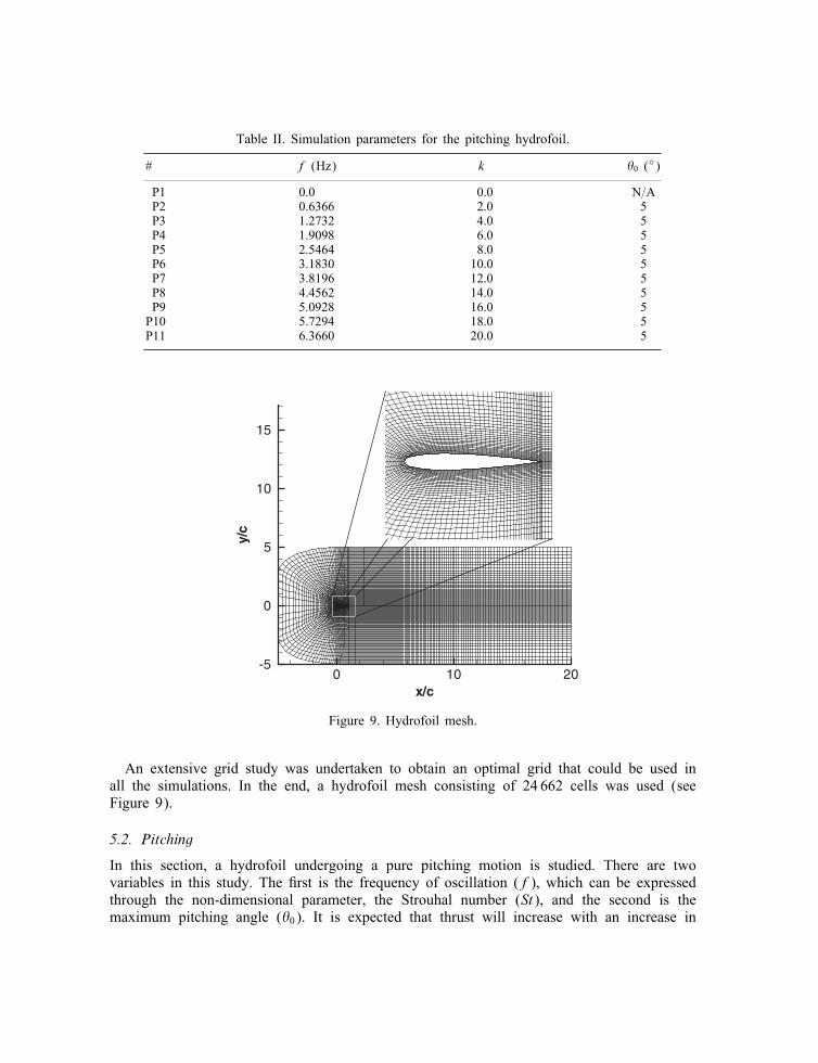
Table II. Simulation parameters for the pitching hydrofoil.

# f (Hz) k �0 (◦)

P1 0.0 0.0 N=AP2 0.6366 2.0 5P3 1.2732 4.0 5P4 1.9098 6.0 5P5 2.5464 8.0 5P6 3.1830 10.0 5P7 3.8196 12.0 5P8 4.4562 14.0 5P9 5.0928 16.0 5P10 5.7294 18.0 5P11 6.3660 20.0 5

x/c

y/c

0 10 20-5

0

5

10

15

Figure 9. Hydrofoil mesh.

An extensive grid study was undertaken to obtain an optimal grid that could be used inall the simulations. In the end, a hydrofoil mesh consisting of 24 662 cells was used (seeFigure 9).

5.2. Pitching

In this section, a hydrofoil undergoing a pure pitching motion is studied. There are twovariables in this study. The �rst is the frequency of oscillation (f), which can be expressedthrough the non-dimensional parameter, the Strouhal number (St), and the second is themaximum pitching angle (�0). It is expected that thrust will increase with an increase in

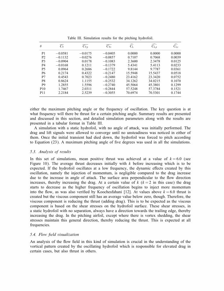
Table III. Simulation results for the pitching hydrofoil.

# CT CTp CTv CL CLp CLv

P1 −0:0581 −0:0175 −0:0405 0.0000 0.0000 0.0000P2 −0:1132 −0:0276 −0:0857 0.7107 0.7068 0.0039P3 −0:0904 0.0178 −0:1083 2.3600 2.3478 0.0125P4 −0:0168 0.1211 −0:1379 5.4341 5.4113 0.0233P5 0.0964 0.2686 −0:1722 9.8144 9.7787 0.0361P6 0.2174 0.4322 −0:2147 15.5948 15.5437 0.0518P7 0.4543 0.7023 −0:2480 23.4162 23.3420 0.0752P8 0.8624 1.1155 −0:2532 34.1262 34.0215 0.1070P9 1.2855 1.5596 −0:2740 45.5064 45.3801 0.1299P10 1.7467 2.0311 −0:2844 57.5248 57.3784 0.1521P11 2.2184 2.5239 −0:3055 70.6974 70.5301 0.1744

either the maximum pitching angle or the frequency of oscillation. The key question is atwhat frequency will there be thrust for a certain pitching angle. Summary results are presentedand discussed in this section, and detailed simulation parameters along with the results arepresented in a tabular format in Table III.A simulation with a static hydrofoil, with no angle of attack, was initially performed. The

drag and lift signals were allowed to converge until no unsteadiness was noticed in either ofthem. Once the initial transient had died down, the hydrofoil was forced to pitch accordingto Equation (23). A maximum pitching angle of �ve degrees was used in all the simulations.

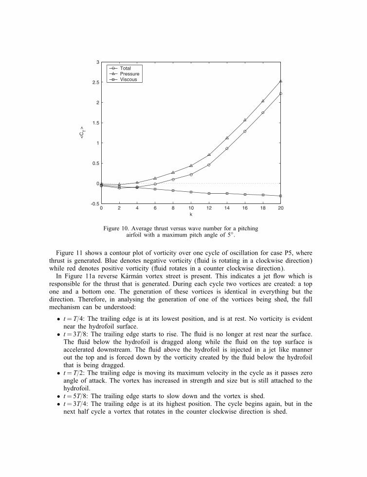
5.3. Analysis of results

In this set of simulations, mean positive thrust was achieved at a value of k=6:0 (seeFigure 10). The average thrust decreases initially with k before increasing which is to beexpected. If the hydrofoil oscillates at a low frequency, the dynamic e�ects created by thisoscillation, namely the injection of momentum, is negligible compared to the drag increasedue to the increase in angle of attack. The surface area perpendicular to the �ow directionincreases, thereby increasing the drag. At a certain value of k (k=2 in this case) the dragstarts to decrease as the higher frequency of oscillation begins to inject more momentuminto the �ow, as was also veri�ed by Koochesfahani [12]. At values above k=6:0 thrust iscreated but the viscous component still has an average value below zero, though. Therefore, theviscous component is reducing the thrust (adding drag). This is to be expected as the viscouscomponent is based on the shear stresses on the hydrofoil surface. These shear stresses, ina static hydrofoil with no separation, always have a direction towards the trailing edge, therebyincreasing the drag. In the pitching airfoil, except where there is vortex shedding, the shearstresses maintain this general direction, thereby reducing the thrust. This is expected at allfrequencies.

5.4. Flow �eld visualization

An analysis of the �ow �eld in this kind of simulation is crucial in the understanding of thevortical pattern created by the oscillating hydrofoil which is responsible for elevated drag incertain cases, but also thrust in others.

0 2 4 6 8 10 12 14 16 18 20-0.5

0

0.5

1

1.5

2

2.5

3

k

<C

T>

TotalPressureViscous

Figure 10. Average thrust versus wave number for a pitchingairfoil with a maximum pitch angle of 5◦.

Figure 11 shows a contour plot of vorticity over one cycle of oscillation for case P5, wherethrust is generated. Blue denotes negative vorticity (�uid is rotating in a clockwise direction)while red denotes positive vorticity (�uid rotates in a counter clockwise direction).In Figure 11a reverse K�arm�an vortex street is present. This indicates a jet �ow which is

responsible for the thrust that is generated. During each cycle two vortices are created: a topone and a bottom one. The generation of these vortices is identical in everything but thedirection. Therefore, in analysing the generation of one of the vortices being shed, the fullmechanism can be understood:

• t=T=4: The trailing edge is at its lowest position, and is at rest. No vorticity is evidentnear the hydrofoil surface.

• t=3T=8: The trailing edge starts to rise. The �uid is no longer at rest near the surface.The �uid below the hydrofoil is dragged along while the �uid on the top surface isaccelerated downstream. The �uid above the hydrofoil is injected in a jet like mannerout the top and is forced down by the vorticity created by the �uid below the hydrofoilthat is being dragged.

• t=T=2: The trailing edge is moving its maximum velocity in the cycle as it passes zeroangle of attack. The vortex has increased in strength and size but is still attached to thehydrofoil.

• t=5T=8: The trailing edge starts to slow down and the vortex is shed.• t=3T=4: The trailing edge is at its highest position. The cycle begins again, but in thenext half cycle a vortex that rotates in the counter clockwise direction is shed.

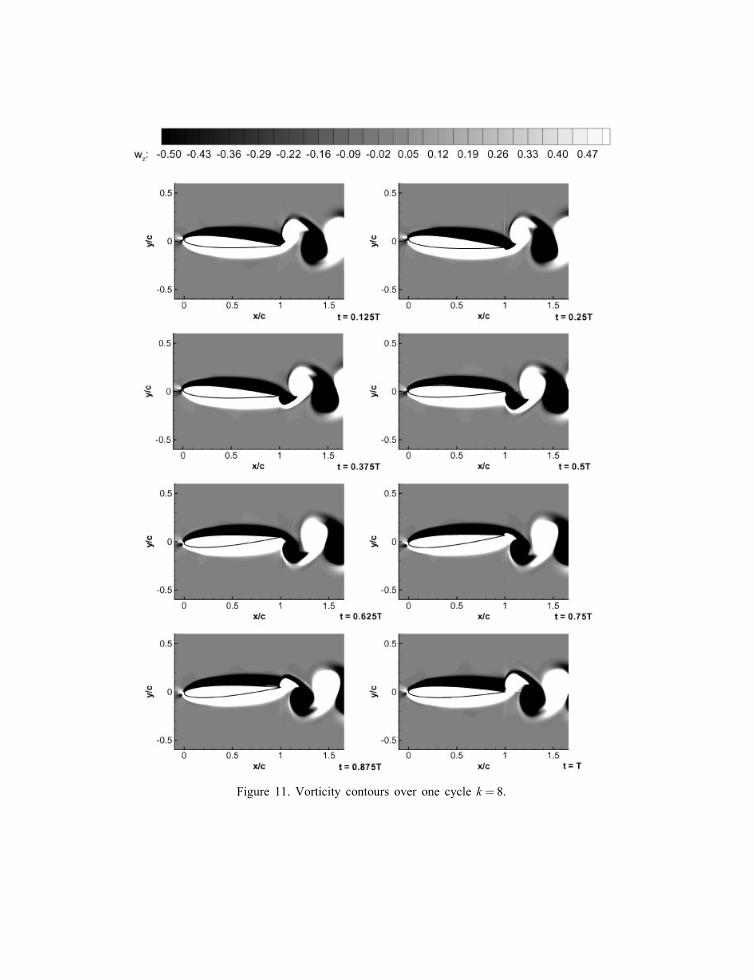
Figure 11. Vorticity contours over one cycle k =8.

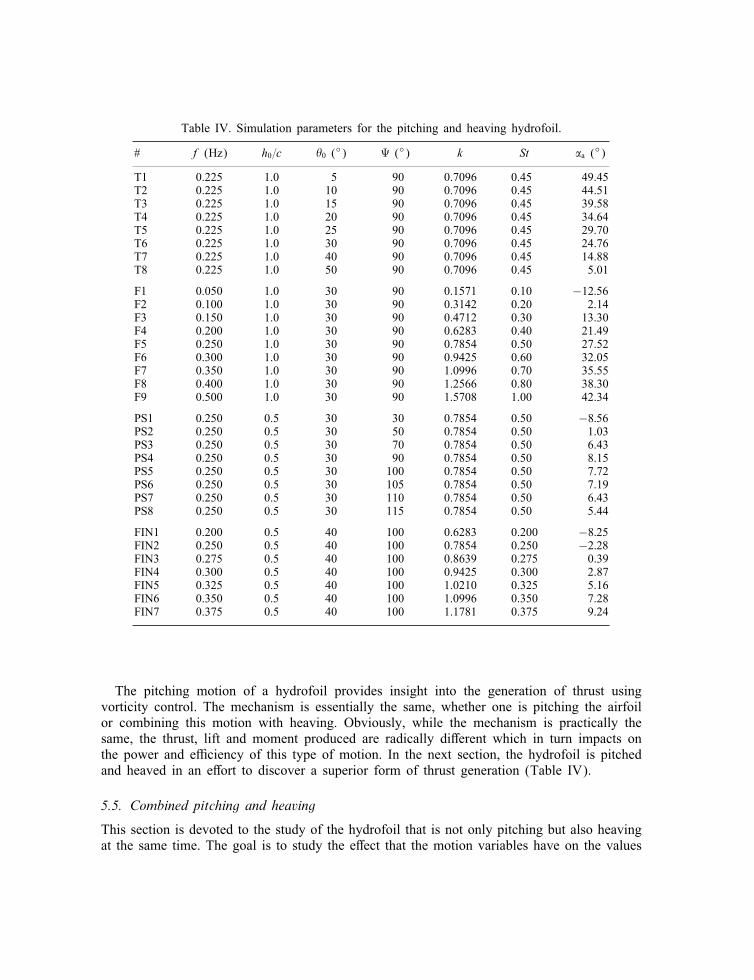
Table IV. Simulation parameters for the pitching and heaving hydrofoil.

# f (Hz) h0=c �0 (◦) � (◦) k St �a (◦)

T1 0.225 1.0 5 90 0.7096 0.45 49.45T2 0.225 1.0 10 90 0.7096 0.45 44.51T3 0.225 1.0 15 90 0.7096 0.45 39.58T4 0.225 1.0 20 90 0.7096 0.45 34.64T5 0.225 1.0 25 90 0.7096 0.45 29.70T6 0.225 1.0 30 90 0.7096 0.45 24.76T7 0.225 1.0 40 90 0.7096 0.45 14.88T8 0.225 1.0 50 90 0.7096 0.45 5.01

F1 0.050 1.0 30 90 0.1571 0.10 −12:56F2 0.100 1.0 30 90 0.3142 0.20 2.14F3 0.150 1.0 30 90 0.4712 0.30 13.30F4 0.200 1.0 30 90 0.6283 0.40 21.49F5 0.250 1.0 30 90 0.7854 0.50 27.52F6 0.300 1.0 30 90 0.9425 0.60 32.05F7 0.350 1.0 30 90 1.0996 0.70 35.55F8 0.400 1.0 30 90 1.2566 0.80 38.30F9 0.500 1.0 30 90 1.5708 1.00 42.34

PS1 0.250 0.5 30 30 0.7854 0.50 −8:56PS2 0.250 0.5 30 50 0.7854 0.50 1.03PS3 0.250 0.5 30 70 0.7854 0.50 6.43PS4 0.250 0.5 30 90 0.7854 0.50 8.15PS5 0.250 0.5 30 100 0.7854 0.50 7.72PS6 0.250 0.5 30 105 0.7854 0.50 7.19PS7 0.250 0.5 30 110 0.7854 0.50 6.43PS8 0.250 0.5 30 115 0.7854 0.50 5.44

FIN1 0.200 0.5 40 100 0.6283 0.200 −8:25FIN2 0.250 0.5 40 100 0.7854 0.250 −2:28FIN3 0.275 0.5 40 100 0.8639 0.275 0.39FIN4 0.300 0.5 40 100 0.9425 0.300 2.87FIN5 0.325 0.5 40 100 1.0210 0.325 5.16FIN6 0.350 0.5 40 100 1.0996 0.350 7.28FIN7 0.375 0.5 40 100 1.1781 0.375 9.24

The pitching motion of a hydrofoil provides insight into the generation of thrust usingvorticity control. The mechanism is essentially the same, whether one is pitching the airfoilor combining this motion with heaving. Obviously, while the mechanism is practically thesame, the thrust, lift and moment produced are radically di�erent which in turn impacts onthe power and e�ciency of this type of motion. In the next section, the hydrofoil is pitchedand heaved in an e�ort to discover a superior form of thrust generation (Table IV).

5.5. Combined pitching and heaving

This section is devoted to the study of the hydrofoil that is not only pitching but also heavingat the same time. The goal is to study the e�ect that the motion variables have on the values

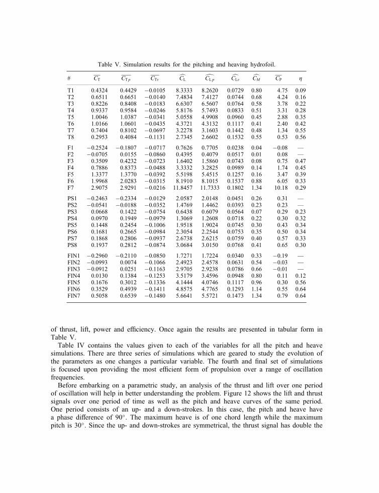
Table V. Simulation results for the pitching and heaving hydrofoil.

# CT CTp CTv CL CLp CLv CM CP �

T1 0.4324 0.4429 −0:0105 8.3333 8.2620 0.0729 0.80 4.75 0.09T2 0.6511 0.6651 −0:0140 7.4834 7.4127 0.0744 0.68 4.24 0.16T3 0.8226 0.8408 −0:0183 6.6307 6.5607 0.0764 0.58 3.78 0.22T4 0.9337 0.9584 −0:0246 5.8176 5.7493 0.0833 0.51 3.31 0.28T5 1.0046 1.0387 −0:0341 5.0558 4.9908 0.0960 0.45 2.88 0.35T6 1.0166 1.0601 −0:0435 4.3721 4.3132 0.1117 0.41 2.40 0.42T7 0.7404 0.8102 −0:0697 3.2278 3.1603 0.1442 0.48 1.34 0.55T8 0.2953 0.4084 −0:1131 2.7345 2.6602 0.1532 0.55 0.53 0.56

F1 −0:2524 −0:1807 −0:0717 0.7626 0.7705 0.0238 0.04 −0:08 —F2 −0:0705 0.0155 −0:0860 0.4395 0.4079 0.0517 0.01 0.08 —F3 0.3509 0.4232 −0:0723 1.6402 1.5860 0.0743 0.08 0.75 0.47F4 0.7886 0.8373 −0:0488 3.3332 3.2825 0.0989 0.14 1.74 0.45F5 1.3377 1.3770 −0:0392 5.5198 5.4515 0.1257 0.16 3.47 0.39F6 1.9968 2.0283 −0:0315 8.1910 8.1015 0.1537 0.88 6.05 0.33F7 2.9075 2.9291 −0:0216 11.8457 11.7333 0.1802 1.34 10.18 0.29

PS1 −0:2463 −0:2334 −0:0129 2.0587 2.0148 0.0451 0.26 0.31 —PS2 −0:0541 −0:0188 −0:0352 1.4769 1.4462 0.0393 0.23 0.23 —PS3 0.0668 0.1422 −0:0754 0.6438 0.6079 0.0564 0.07 0.29 0.23PS4 0.0970 0.1949 −0:0979 1.3069 1.2608 0.0718 0.22 0.30 0.32PS5 0.1448 0.2454 −0:1006 1.9518 1.9024 0.0745 0.30 0.43 0.34PS6 0.1681 0.2665 −0:0984 2.3054 2.2544 0.0753 0.35 0.50 0.34PS7 0.1868 0.2806 −0:0937 2.6738 2.6215 0.0759 0.40 0.57 0.33PS8 0.1937 0.2812 −0:0874 3.0684 3.0150 0.0768 0.41 0.65 0.30

FIN1 −0:2960 −0:2110 −0:0850 1.7271 1.7224 0.0340 0.33 −0:19 —FIN2 −0:0993 0.0074 −0:1066 2.4923 2.4578 0.0631 0.54 −0:03 —FIN3 −0:0912 0.0251 −0:1163 2.9705 2.9238 0.0786 0.66 −0:01 —FIN4 0.0130 0.1384 −0:1253 3.5179 3.4596 0.0948 0.80 0.11 0.12FIN5 0.1676 0.3012 −0:1336 4.1444 4.0746 0.1117 0.96 0.30 0.56FIN6 0.3529 0.4939 −0:1411 4.8575 4.7765 0.1293 1.14 0.55 0.64FIN7 0.5058 0.6539 −0:1480 5.6641 5.5721 0.1473 1.34 0.79 0.64

of thrust, lift, power and e�ciency. Once again the results are presented in tabular form inTable V.Table IV contains the values given to each of the variables for all the pitch and heave

simulations. There are three series of simulations which are geared to study the evolution ofthe parameters as one changes a particular variable. The fourth and �nal set of simulationsis focused upon providing the most e�cient form of propulsion over a range of oscillationfrequencies.Before embarking on a parametric study, an analysis of the thrust and lift over one period

of oscillation will help in better understanding the problem. Figure 12 shows the lift and thrustsignals over one period of time as well as the pitch and heave curves of the same period.One period consists of an up- and a down-strokes. In this case, the pitch and heave havea phase di�erence of 90◦. The maximum heave is of one chord length while the maximumpitch is 30◦. Since the up- and down-strokes are symmetrical, the thrust signal has double the

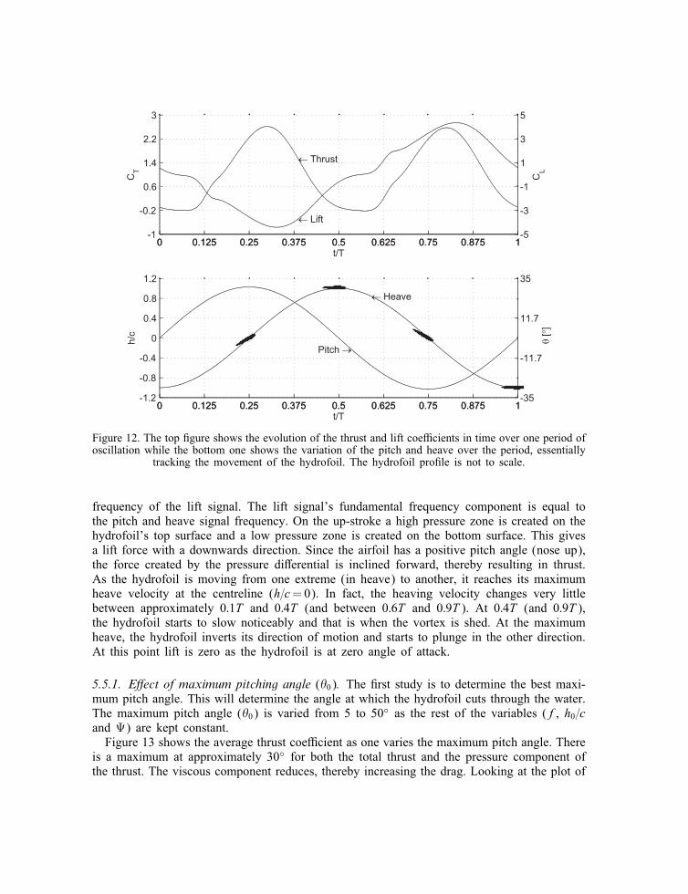
Figure 12. The top �gure shows the evolution of the thrust and lift coe�cients in time over one period ofoscillation while the bottom one shows the variation of the pitch and heave over the period, essentially

tracking the movement of the hydrofoil. The hydrofoil pro�le is not to scale.

frequency of the lift signal. The lift signal’s fundamental frequency component is equal tothe pitch and heave signal frequency. On the up-stroke a high pressure zone is created on thehydrofoil’s top surface and a low pressure zone is created on the bottom surface. This givesa lift force with a downwards direction. Since the airfoil has a positive pitch angle (nose up),the force created by the pressure di�erential is inclined forward, thereby resulting in thrust.As the hydrofoil is moving from one extreme (in heave) to another, it reaches its maximumheave velocity at the centreline (h=c=0). In fact, the heaving velocity changes very littlebetween approximately 0:1T and 0:4T (and between 0:6T and 0:9T ). At 0:4T (and 0:9T ),the hydrofoil starts to slow noticeably and that is when the vortex is shed. At the maximumheave, the hydrofoil inverts its direction of motion and starts to plunge in the other direction.At this point lift is zero as the hydrofoil is at zero angle of attack.

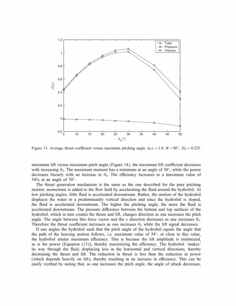
5.5.1. E�ect of maximum pitching angle (�0). The �rst study is to determine the best maxi-mum pitch angle. This will determine the angle at which the hydrofoil cuts through the water.The maximum pitch angle (�0) is varied from 5 to 50◦ as the rest of the variables (f, h0=cand �) are kept constant.Figure 13 shows the average thrust coe�cient as one varies the maximum pitch angle. There

is a maximum at approximately 30◦ for both the total thrust and the pressure component ofthe thrust. The viscous component reduces, thereby increasing the drag. Looking at the plot of

5 10 15 20 25 30 35 40 45 50-0.2

0

0.2

0.4

0.6

0.8

1

1.2

0 [ θ °]

<C

T>

TotalPressureViscous

Figure 13. Average thrust coe�cient versus maximum pitching angle; h0=c=1:0, �=90◦, Sth=0:225.

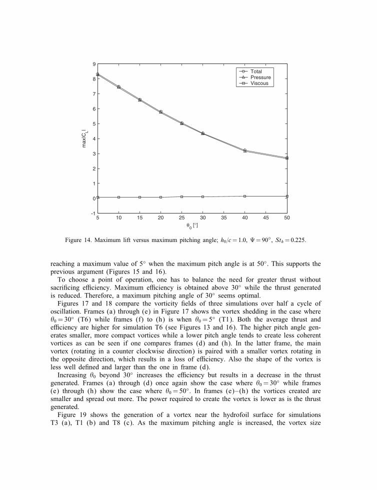
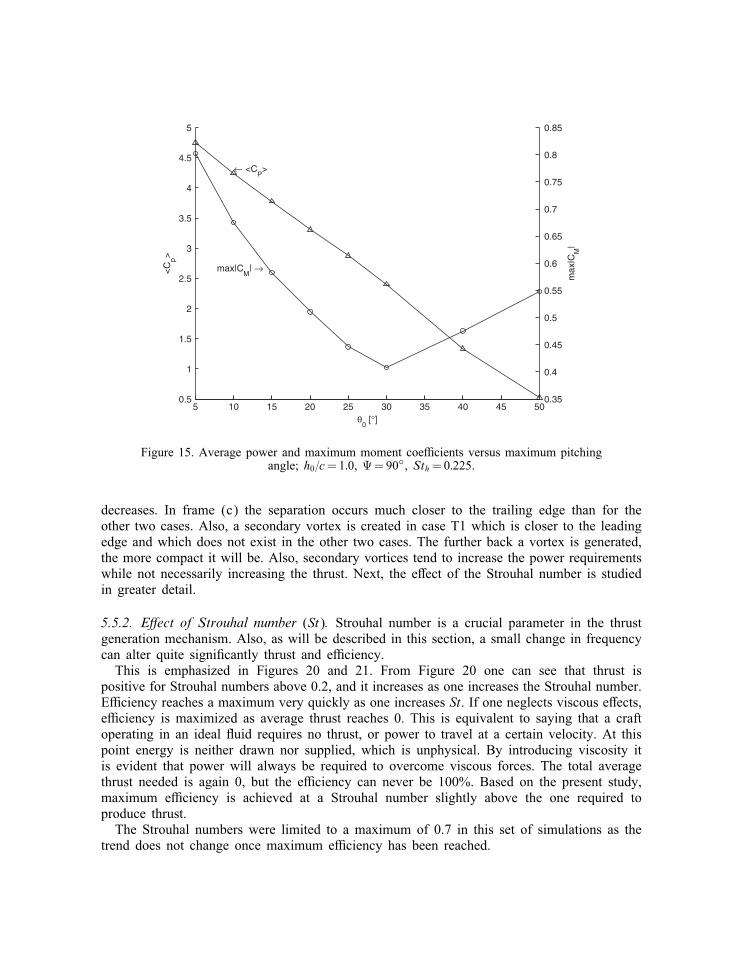
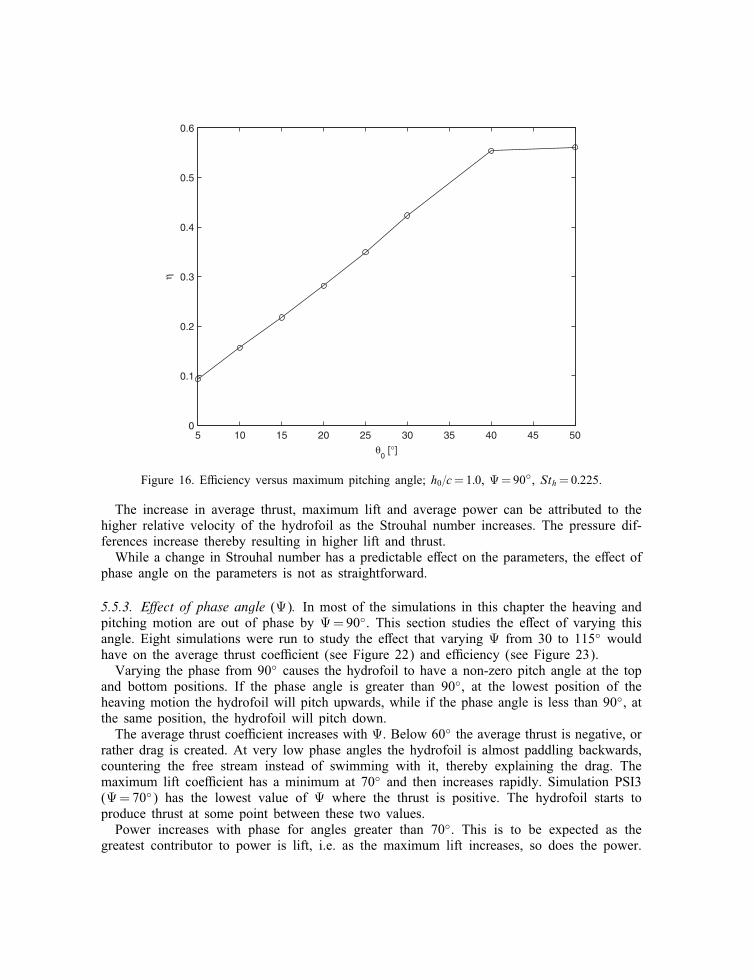
maximum lift versus maximum pitch angle (Figure 14), the maximum lift coe�cient decreaseswith increasing �0. The maximum moment has a minimum at an angle of 30◦, while the powerdecreases linearly with an increase in �0. The e�ciency increases to a maximum value of54% at an angle of 50◦.The thrust generation mechanism is the same as the one described for the pure pitching

motion: momentum is added to the �ow �eld by accelerating the �uid around the hydrofoil. Atlow pitching angles, little �uid is accelerated downstream. Rather, the motion of the hydrofoildisplaces the water in a predominantly vertical direction and since the hydrofoil is sloped,the �uid is accelerated downstream. The higher the pitching angle, the more the �uid isaccelerated downstream. The pressure di�erence between the bottom and top surfaces of thehydrofoil, which in turn creates the thrust and lift, changes direction as one increases the pitchangle. The angle between this force vector and the x direction decreases as one increases �0.Therefore the thrust coe�cient increases as one increases �0 while the lift signal decreases.If one angles the hydrofoil such that the pitch angle of the hydrofoil equals the angle that

the path of the heaving motion follows, i.e. maximum value of 54◦, or close to this value,the hydrofoil attains maximum e�ciency. This is because the lift amplitude is minimized,as is the power (Equation (13)), thereby maximizing the e�ciency. The hydrofoil ‘snakes’its way through the �uid, displacing less in the horizontal and vertical directions, therebydecreasing the thrust and lift. The reduction in thrust is less than the reduction in power(which depends heavily on lift), thereby resulting in an increase in e�ciency. This can beeasily veri�ed by noting that, as one increases the pitch angle, the angle of attack decreases,

5 10 15 20 25 30 35 40 45 50 -1

0

1

2

3

4

5

6

7

8

9

0 [ θ °]

max

|CL|

TotalPressureViscous

Figure 14. Maximum lift versus maximum pitching angle; h0=c=1:0, �=90◦, Sth=0:225.

reaching a maximum value of 5◦ when the maximum pitch angle is at 50◦. This supports theprevious argument (Figures 15 and 16).To choose a point of operation, one has to balance the need for greater thrust without

sacri�cing e�ciency. Maximum e�ciency is obtained above 30◦ while the thrust generatedis reduced. Therefore, a maximum pitching angle of 30◦ seems optimal.Figures 17 and 18 compare the vorticity �elds of three simulations over half a cycle of

oscillation. Frames (a) through (e) in Figure 17 shows the vortex shedding in the case where�0 = 30◦ (T6) while frames (f) to (h) is when �0 = 5◦ (T1). Both the average thrust ande�ciency are higher for simulation T6 (see Figures 13 and 16). The higher pitch angle gen-erates smaller, more compact vortices while a lower pitch angle tends to create less coherentvortices as can be seen if one compares frames (d) and (h). In the latter frame, the mainvortex (rotating in a counter clockwise direction) is paired with a smaller vortex rotating inthe opposite direction, which results in a loss of e�ciency. Also the shape of the vortex isless well de�ned and larger than the one in frame (d).Increasing �0 beyond 30◦ increases the e�ciency but results in a decrease in the thrust

generated. Frames (a) through (d) once again show the case where �0 = 30◦ while frames(e) through (h) show the case where �0 = 50◦. In frames (e)–(h) the vortices created aresmaller and spread out more. The power required to create the vortex is lower as is the thrustgenerated.Figure 19 shows the generation of a vortex near the hydrofoil surface for simulations

T3 (a), T1 (b) and T8 (c). As the maximum pitching angle is increased, the vortex size

5 10 15 20 25 30 35 40 45 500.5

1

1.5

2

2.5

3

3.5

4

4.5

5

<C

p>← <C

P>

0.35

0.4

0.45

0.5

0.55

0.6

0.65

0.7

0.75

0.8

0.85

max|CM

| →

0 [ θ °]

max

|CM

|

Figure 15. Average power and maximum moment coe�cients versus maximum pitchingangle; h0=c=1:0, �=90◦, Sth=0:225.

decreases. In frame (c) the separation occurs much closer to the trailing edge than for theother two cases. Also, a secondary vortex is created in case T1 which is closer to the leadingedge and which does not exist in the other two cases. The further back a vortex is generated,the more compact it will be. Also, secondary vortices tend to increase the power requirementswhile not necessarily increasing the thrust. Next, the e�ect of the Strouhal number is studiedin greater detail.

5.5.2. E�ect of Strouhal number (St). Strouhal number is a crucial parameter in the thrustgeneration mechanism. Also, as will be described in this section, a small change in frequencycan alter quite signi�cantly thrust and e�ciency.This is emphasized in Figures 20 and 21. From Figure 20 one can see that thrust is

positive for Strouhal numbers above 0.2, and it increases as one increases the Strouhal number.E�ciency reaches a maximum very quickly as one increases St. If one neglects viscous e�ects,e�ciency is maximized as average thrust reaches 0. This is equivalent to saying that a craftoperating in an ideal �uid requires no thrust, or power to travel at a certain velocity. At thispoint energy is neither drawn nor supplied, which is unphysical. By introducing viscosity itis evident that power will always be required to overcome viscous forces. The total averagethrust needed is again 0, but the e�ciency can never be 100%. Based on the present study,maximum e�ciency is achieved at a Strouhal number slightly above the one required toproduce thrust.The Strouhal numbers were limited to a maximum of 0.7 in this set of simulations as the

trend does not change once maximum e�ciency has been reached.

5 10 15 20 25 30 35 40 45 500

0.1

0.2

0.3

0.4

0.5

0.6

θ0 [°]

η

Figure 16. E�ciency versus maximum pitching angle; h0=c=1:0, �=90◦, Sth=0:225.

The increase in average thrust, maximum lift and average power can be attributed to thehigher relative velocity of the hydrofoil as the Strouhal number increases. The pressure dif-ferences increase thereby resulting in higher lift and thrust.While a change in Strouhal number has a predictable e�ect on the parameters, the e�ect of

phase angle on the parameters is not as straightforward.

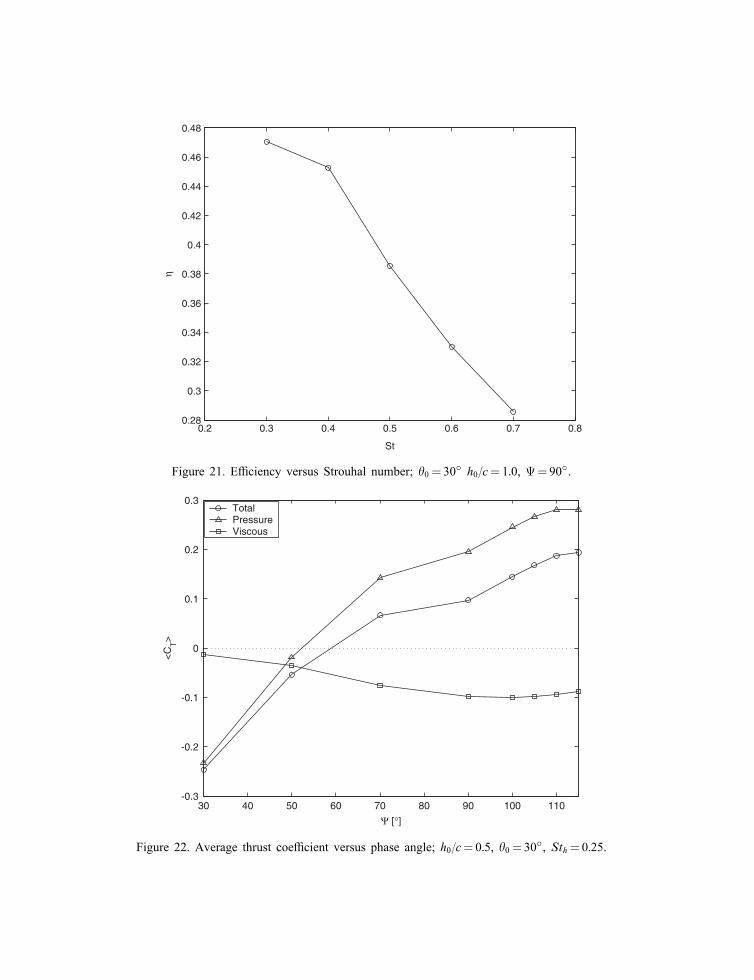
5.5.3. E�ect of phase angle (�). In most of the simulations in this chapter the heaving andpitching motion are out of phase by �=90◦. This section studies the e�ect of varying thisangle. Eight simulations were run to study the e�ect that varying � from 30 to 115◦ wouldhave on the average thrust coe�cient (see Figure 22) and e�ciency (see Figure 23).Varying the phase from 90◦ causes the hydrofoil to have a non-zero pitch angle at the top

and bottom positions. If the phase angle is greater than 90◦, at the lowest position of theheaving motion the hydrofoil will pitch upwards, while if the phase angle is less than 90◦, atthe same position, the hydrofoil will pitch down.The average thrust coe�cient increases with �. Below 60◦ the average thrust is negative, or

rather drag is created. At very low phase angles the hydrofoil is almost paddling backwards,countering the free stream instead of swimming with it, thereby explaining the drag. Themaximum lift coe�cient has a minimum at 70◦ and then increases rapidly. Simulation PSI3(�=70◦) has the lowest value of � where the thrust is positive. The hydrofoil starts toproduce thrust at some point between these two values.Power increases with phase for angles greater than 70◦. This is to be expected as the

greatest contributor to power is lift, i.e. as the maximum lift increases, so does the power.

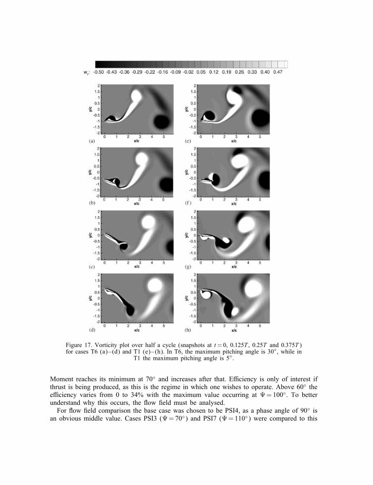
Figure 17. Vorticity plot over half a cycle (snapshots at t=0, 0:125T , 0:25T and 0:375T )for cases T6 (a)–(d) and T1 (e)–(h). In T6, the maximum pitching angle is 30◦, while in

T1 the maximum pitching angle is 5◦.

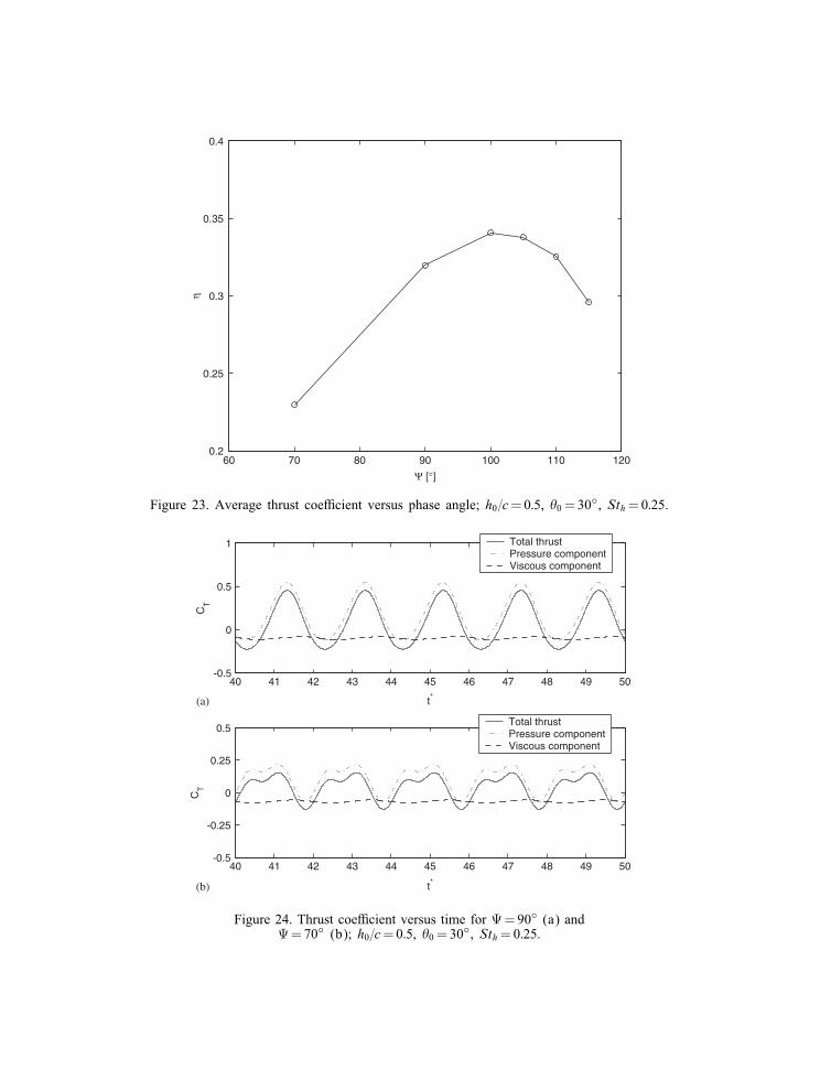
Moment reaches its minimum at 70◦ and increases after that. E�ciency is only of interest ifthrust is being produced, as this is the regime in which one wishes to operate. Above 60◦ thee�ciency varies from 0 to 34% with the maximum value occurring at �=100◦. To betterunderstand why this occurs, the �ow �eld must be analysed.For �ow �eld comparison the base case was chosen to be PSI4, as a phase angle of 90◦ is

an obvious middle value. Cases PSI3 (�=70◦) and PSI7 (�=110◦) were compared to this

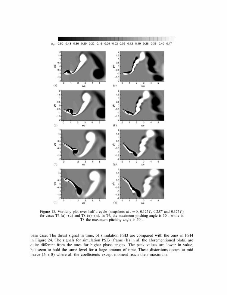
Figure 18. Vorticity plot over half a cycle (snapshots at t=0, 0:125T , 0:25T and 0:375T )for cases T6 (a)–(d) and T8 (e)–(h). In T6, the maximum pitching angle is 30◦, while in

T8 the maximum pitching angle is 50◦.

base case. The thrust signal in time, of simulation PSI3 are compared with the ones in PSI4in Figure 24. The signals for simulation PSI3 (frame (b) in all the aforementioned plots) arequite di�erent from the ones for higher phase angles. The peak values are lower in value,but seem to hold the same level for a large amount of time. These distortions occurs at midheave (h ≈ 0) where all the coe�cients except moment reach their maximum.

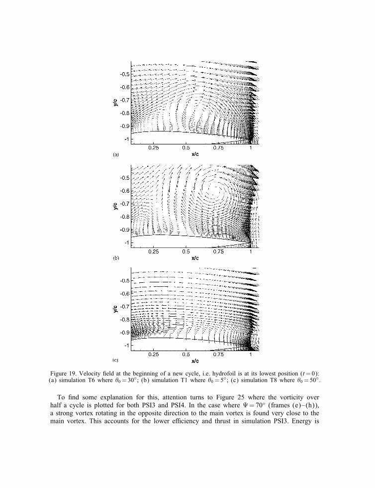
Figure 19. Velocity �eld at the beginning of a new cycle, i.e. hydrofoil is at its lowest position (t=0):(a) simulation T6 where �0 = 30◦; (b) simulation T1 where �0 = 5◦; (c) simulation T8 where �0 = 50◦.

To �nd some explanation for this, attention turns to Figure 25 where the vorticity overhalf a cycle is plotted for both PSI3 and PSI4. In the case where �=70◦ (frames (e)–(h)),a strong vortex rotating in the opposite direction to the main vortex is found very close to themain vortex. This accounts for the lower e�ciency and thrust in simulation PSI3. Energy is

0.1 0.2 0.3 0.4 0.5 0.6 0.7-0.5

0

0.5

1

1.5

2

2.5

3

St

<C

T>

TotalPressureViscous

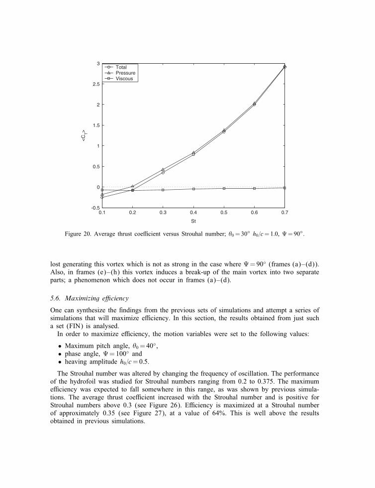
Figure 20. Average thrust coe�cient versus Strouhal number; �0 = 30◦ h0=c=1:0, �=90◦.

lost generating this vortex which is not as strong in the case where �=90◦ (frames (a)–(d)).Also, in frames (e)–(h) this vortex induces a break-up of the main vortex into two separateparts; a phenomenon which does not occur in frames (a)–(d).

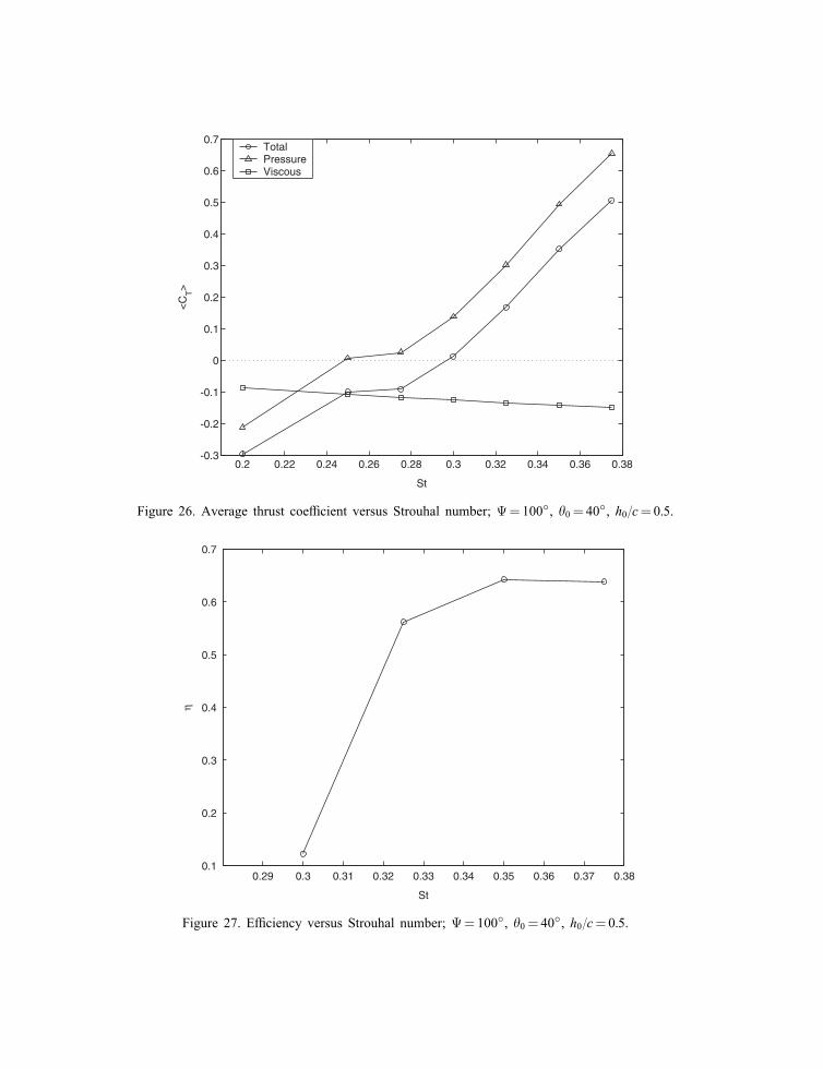
5.6. Maximizing e�ciency

One can synthesize the �ndings from the previous sets of simulations and attempt a series ofsimulations that will maximize e�ciency. In this section, the results obtained from just sucha set (FIN) is analysed.In order to maximize e�ciency, the motion variables were set to the following values:

• Maximum pitch angle, �0 = 40◦,• phase angle, �=100◦ and• heaving amplitude h0=c=0:5.The Strouhal number was altered by changing the frequency of oscillation. The performance

of the hydrofoil was studied for Strouhal numbers ranging from 0.2 to 0.375. The maximume�ciency was expected to fall somewhere in this range, as was shown by previous simula-tions. The average thrust coe�cient increased with the Strouhal number and is positive forStrouhal numbers above 0.3 (see Figure 26). E�ciency is maximized at a Strouhal numberof approximately 0.35 (see Figure 27), at a value of 64%. This is well above the resultsobtained in previous simulations.

0.2 0.3 0.4 0.5 0.6 0.7 0.80.28

0.3

0.32

0.34

0.36

0.38

0.4

0.42

0.44

0.46

0.48

St

η

Figure 21. E�ciency versus Strouhal number; �0 = 30◦ h0=c=1:0, �=90◦.

30 40 50 60 70 80 90 100 110-0.3

-0.2

-0.1

0

0.1

0.2

0.3

Ψ [°]

<C

T>

TotalPressureViscous

Figure 22. Average thrust coe�cient versus phase angle; h0=c=0:5, �0 = 30◦, Sth=0:25.

60 70 80 90 100 110 1200.2

0.25

0.3

0.35

0.4

Ψ [°]

η

Figure 23. Average thrust coe�cient versus phase angle; h0=c=0:5, �0 = 30◦, Sth=0:25.

40 41 42 43 44 45 46 47 48 49 50-0.5

0

0.5

1

t*

CT

Total thrustPressure componentViscous component

40 41 42 43 44 45 46 47 48 49 50-0.5

-0.25

0

0.25

0.5

t*

CT

Total thrustPressure componentViscous component

(a)

(b)

Figure 24. Thrust coe�cient versus time for �=90◦ (a) and�=70◦ (b); h0=c=0:5, �0 = 30◦, Sth=0:25.

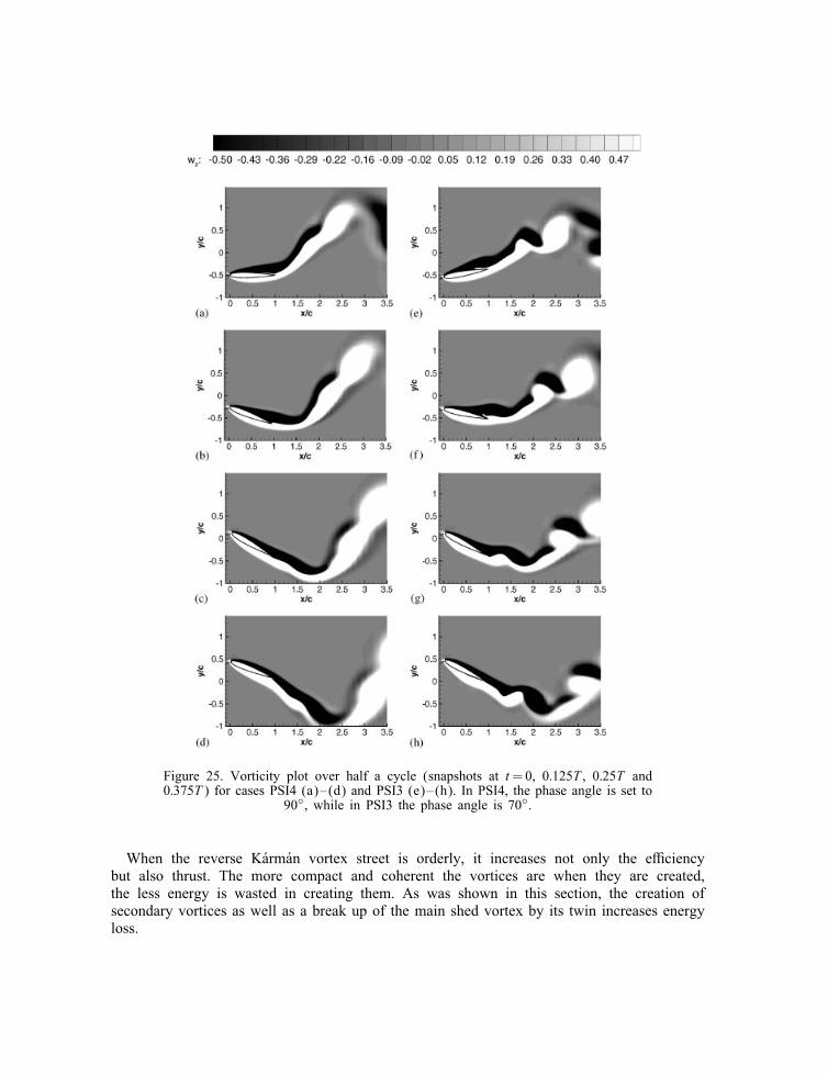
Figure 25. Vorticity plot over half a cycle (snapshots at t=0, 0:125T , 0:25T and0:375T ) for cases PSI4 (a)–(d) and PSI3 (e)–(h). In PSI4, the phase angle is set to

90◦, while in PSI3 the phase angle is 70◦.

When the reverse K�arm�an vortex street is orderly, it increases not only the e�ciencybut also thrust. The more compact and coherent the vortices are when they are created,the less energy is wasted in creating them. As was shown in this section, the creation ofsecondary vortices as well as a break up of the main shed vortex by its twin increases energyloss.

0.2 0.22 0.24 0.26 0.28 0.3 0.32 0.34 0.36 0.38-0.3

-0.2

-0.1

0

0.1

0.2

0.3

0.4

0.5

0.6

0.7

St

<C

T>

TotalPressureViscous

Figure 26. Average thrust coe�cient versus Strouhal number; �=100◦, �0 = 40◦, h0=c=0:5.

0.29 0.3 0.31 0.32 0.33 0.34 0.35 0.36 0.37 0.380.1

0.2

0.3

0.4

0.5

0.6

0.7

St

η

Figure 27. E�ciency versus Strouhal number; �=100◦, �0 = 40◦, h0=c=0:5.

Some of the simulations performed in this chapter can be directly compared with resultsobtained in Anderson’s study of �apping hydrofoils [17, 28]. Her study consisted of towinga hydrofoil undergoing a pitching and heaving motion. Two Reynolds number were considered:40 000 and 1100. In the former, it was possible to measure the moment on the hydrofoil andthe associated power and e�ciency. In the lower Reynolds number case, this was not done andcomparison to our simulations is only possible for thrust. In all cases, the present study under-predicted the thrust from about 15–40% in the worst case. The discrepancies are attributedto some extent to insu�cient grid re�nement, but primarily to three-dimensional e�ects thatare not accounted for in the present simulations.

6. CONCLUSIONS

The CFD-based method is an excellent numerical tool to solve the �ow �eld using the fullNavier–Stokes equations and complex geometries can be easily incorporated. With these ad-vantages comes greater computational e�ort and the need for a more judicious choice ofsimulation parameters. The mechanism of thrust generated by a �apping hydrofoil was rep-resented by a two-dimensional �ow at low Reynolds numbers. In this range, smaller gridscan be used to reduce the computational time needed to solve the �ow �eld. A drawbackin simulating �ows at low Reynolds numbers is that the viscous forces are overestimated inrelation to the high Reynolds number �ows calculations. At a Reynolds number in which thecraft will operate thrust and lift forces due to viscosity are very small compared to the inertialforces. This means that the maximum e�ciency calculated can be improved upon by simplyincreasing the Reynolds number. Experimental tests by Anderson et al. [17] at a Reynoldsnumber of 40 000 shows runs with 90% e�ciency, thus validating this observation.The code validation was performed using an oscillating cylinder in a cross-�ow. This type

of �ow is similar to the one generated by the oscillating hydrofoil, as shown in the �owvisualization results. Also, this benchmark case helped validate the ALE algorithm close tosolid boundaries. The results reported in the literature for this case vary considerably howeverCFDLIB produced results which �tted into the solution set.The results obtained show the sensitivity of thrust and e�ciency to the Strouhal number,

maximum pitch angle and phase angle. This is an important result that has to be taken intoaccount when designing the prototype. A design trade-o� was found between the e�ciencyand generated thrust. Although e�ciency is an obvious parameter to maximize, one mightnot want to do it at a cost of reducing thrust, as acceleration is often an important designconsideration in the operational envelope of the undersea vehicle.The simulations revealed that the maximum lift coe�cient decreases with increasing pitch

angle. The operation point was selected based on the need for greater thrust without sacri-�cing e�ciency. A maximum pitching angle of 30◦ was found to be optimal. It was foundthat a small variation in oscillation frequency considerably a�ected thrust and e�ciency. Anincrease in oscillation frequency resulted in an increase in average thrust, maximum lift andaverage power. The e�ect of phase angle between the heaving and pitching motions was stud-ied as well. It was found that the average thrust coe�cient increases with the phase angle.Below 60◦ the average thrust is negative, resulting in drag. The maximum lift coe�cient hasa minimum at 70◦ and then it increases rapidly while the thrust is positive. The hydrofoilwas found to generate positive thrust between these two operating values. The performance

of the hydrofoil does not depend on the heaving frequency and amplitude, however it wasfound to depend on the Strouhal number. A small variation in the Strouhal number can havean extremely large e�ect on the thrust and e�ciency.Finally, the e�ciency was maximized based on the simulations results from the parametric

analysis. In order to maximize e�ciency, the design variables were set at the optimum val-ues, i.e. maximum pitching angle at 40◦, phase angle at 100◦ and non-dimensional heavingamplitude at 0.5. The Strouhal number was varied by changing the oscillation frequency. Itwas found that e�ciency was a maximum at a Strouhal number of 0.35, with a value of 64%.

REFERENCES

1. Triantafyllou GS, Triantafyllou MS, Grosenbaugh MA. Optimal thrust development in oscillating foils withapplication to �sh propulsion. Journal of Fluids and Structures 1993; 7:205–225.

2. Lighthill MJ. Note on the swimming of slender �sh. Journal of Fluid Mechanics 1960; 9:305–317.3. Katz J, Weihs D. Hydrodynamic propulsion by large amplitude oscillation of an airfoil with chordwise �exibility.Journal of Fluid Mechanics 1978; 88:485–497.

4. Wu TY. Swimming of a waving plate. Journal of Fluid Mechanics 1961; 10:321–344.5. Siekmann J. Theoretical studies of sea animal locomotion, Part I. Ingenieur-Archiv 1962; 31:214–228.6. Uldrick JP, Siekmann J. On the swimming of a �exible plate of arbitrary �nite thickness. Journal of FluidMechanics 1964; 20:1–33.

7. Wu TY. Hydromechanics of swimming propulsion. Part 1. Swimming of a two-dimensional �exible plate atvariable speeds in an inviscid �uid. Journal of Fluid Mechanics 1971; 46:337–355.

8. Wu TY. Hydromechanics of swimming propulsion. Part 2. Some optimum shape problems. Journal of FluidMechanics 1971; 46:521–544.

9. Cheng JY, Zhuang LX, Tong BG. Analysis of swimming three-dimensional plates. Journal of Fluid Mechanics1991; 232:341–355.

10. Bandyopadhyay PR, Castano JM, Rice JQ, Philips RB, Nedderman WH, Macy WK. Low-speed maneuveringhydrodynamics of �sh and small underwater vehicles. Journal of Fluids Engineering—Transactions of theAmerican Society of Mechanical Engineers 1997; 119:136–144.

11. Isshiki H, Murakami M. A theory of wave devouring propulsion. Society of Naval Architects of Japan 1984;156:102–114.

12. Koochesfahani M. Vortical patterns in the wake of an oscillating airfoil. AIAA Journal 1989; 27:1200–1205.13. Triantafyllou MS, Triantafyllou GS, Gopalkrishnan R. Wake mechanics for thrust generation in oscillating foils.

Physics of Fluids A 1991; 3(12):2835–2837.14. Gopalkrishnan R, Triantafyllou MS, Triantafyllou GS, Barrett D. Active vorticity control in a shear �ow using

a �apping foil. Journal of Fluid Mechanics 1994; 274:1–21.15. Ramamurti R, Sandberg W, L�hner R. Simulation of �ow about �apping airfoils using a �nite element

incompressible �ow solver. In 37th AIAA Aerospace Sciences Meeting and Exhibit, American Institute ofAeronautics and Astronautics, Reno, NV, 1999.

16. Tuncer IH, Platzer MF. Computational study of �apping airfoil aerodynamics. Journal of Aircraft 2000;37(3):514–520.

17. Anderson JM. Vorticity control for e�cient propulsion. PhD thesis, Massachusetts Institute of Techno-logy=Woods Hole Oceanographic Institution, 1996, pp. 83–145.

18. Stix G. RoboT. Scienti�c American 1994; 270.19. Brackbill JU, Johnson NL, Kashiwa BA, Vanderheyden WB (eds). Workshop: Multi-Phase Flows and Particle

Methods. CFD Society of Canada: Victoria, BC, 1997.20. Blackburn HM, Henderson RD. A study of two-dimensional �ow past an oscillating cylinder. Journal of Fluid

Mechanics 1999; 385:255–286.21. Mendes PA, Branco FA. Analysis of �uid–structure interaction by an arbitrary Lagrangian–Eulerian �nite

element formulation. International Journal for Numerical Methods in Fluids 1999; 30:897–919.

22. Koopman GH. The vortex wakes of vibrating cylinders at low Reynolds numbers. Journal of Fluid Mechanics1967; 28:501–512.

23. Tanida Y, Okajima A, Watanabe Y. Stability of a circular cylinder oscillating in uniform �ow or in a wake.Journal of Fluid Mechanics 1973; 61(4):769–784.

24. Mittal S, Tezduyar TE. A �nite element study of incompressible �ows past oscillating cylinders and aerofoils.International Journal for Numerical Methods in Fluids 1992; 15(9):1073–1118.

25. Mittal S, Tezduyar TE. Massively parallel �nite element computation of incompressible �ows involving �uid-body interactions. Computer Methods in Applied Mechanics and Engineering 1994; 21(3–4):253–282.

26. Tezduyar TE. Parallel �nite element simulation of 3D incompressible �ows: �uid–structure interactions.International Journal for Numerical Methods in Fluids 1995; 21(10):933–953.

27. Hirt CW, Amsden AA, Cook JL. An arbitrary Lagrangian–Eulerian computing method for all �ow speeds.Journal of Computational Physics 1974; 14.

28. Anderson JM, Streitlien K, Barrett DS, Triantafyllou MS. Oscillating foils of high propulsive e�ciency. Journalof Fluid Mechanics 1998; 360:41–72.