ACTAUNIVERSITATIS

UPSALIENSISUPPSALA

2014

Digital Comprehensive Summaries of Uppsala Dissertationsfrom the Faculty of Science and Technology 1118

Adsorption Studies with LiquidChromatography

Experimental Preparations for ThoroughDetermination of Adsorption Data

LENA EDSTRÖM

ISSN 1651-6214ISBN 978-91-554-8858-1urn:nbn:se:uu:diva-216235

Dissertation presented at Uppsala University to be publicly examined in B22, BMC,Husargatan 3, Uppsala, Friday, 14 March 2014 at 10:15 for the degree of Doctor ofPhilosophy. The examination will be conducted in English. Faculty examiner: AssociateProfessor Lars Hagel.

AbstractEdström, L. 2014. Adsorption Studies with Liquid Chromatography. ExperimentalPreparations for Thorough Determination of Adsorption Data. Digital ComprehensiveSummaries of Uppsala Dissertations from the Faculty of Science and Technology 1118. 56 pp.Uppsala: Acta Universitatis Upsaliensis. ISBN 978-91-554-8858-1.

Analytical chemistry is a field with a vast variety of applications. A robust companion inthe field is liquid chromatography, the method used in this thesis, which is an establishedworkhorse and a versatile tool in many different disciplines. It can be used for identificationand quantification of interesting compounds generally present in low concentrations, calledanalytical scale chromatography. It can also be used for isolation and purification of high valuecompounds, called preparative chromatography. The latter is usually conducted in large scalewith high concentrations. With high concentrations it is also possible to determine somethingcalled adsorption isotherms.

Determination of adsorption isotherms is a useful tool for quite a wide variety ofreasons. It can be used for characterisation of chromatographic separation systems, andthen gives information on the retention mechanism as well as provides the possibility tostudy column-column and batch-batch reproducibility. If a protein is immobilised on a solidsupport, adsorption isotherms can be used for pharmacological characterisation of drug-protein interactions. Moreover, they can be used for the study of unexpected chromatographicphenomena.

If the adsorption isotherm is known it is also possible to simulate chromatograms, andsubsequently optimise the separation process numerically. The gain of a numerically optimisedseparation process is higher purity or yield of valuable compounds such as pharmaceuticals orantioxidants, as well as reducing the solvent usage. Taken all together, it saves time, money andthe environment.

However, the process of the adsorption isotherm determination requires a number of carefulexperimental considerations and preparations, and these are the main focus of the thesis.Important steps along the way include the choice of separation system and of suitable analytes,preparation of mobile phases and sample solutions, calibration, determination of injectionprofiles and column void, and of course the adsorption isotherm determination method itself.It is also important to keep track of parameters such as temperature and pH. These issues arediscussed in this thesis.

At the end, a description of useful methods for processing of the raw adsorption isotherm datais presented, as well as a brief passage on methods for numerical optimisation.

Keywords: Liquid chromatography, HPLC, UHPLC, Reversed phase, Preparativechromatography, Adsorption isotherm, Injection profile, Sample pH, pH stable conditions,Peak deformation, Band distortion, Overloaded band, Chiral preparative chromatography

Lena Edström, Department of Chemistry - BMC, Analytical Chemistry, Box 576, UppsalaUniversity, SE-75123 Uppsala, Sweden.

© Lena Edström 2014

ISSN 1651-6214ISBN 978-91-554-8858-1urn:nbn:se:uu:diva-216235 (http://urn.kb.se/resolve?urn=urn:nbn:se:uu:diva-216235)

“Ignorance more frequently begetsconfidence than does knowledge”

Charles Darwin

List of Papers

This thesis is based on the following papers, which are referred to in the text by their Roman numerals.

I. Samuelsson, J., Edström, L., Forssén, P., Fornstedt, T. Injection profiles in liquid chromatography. I. A fundamental investi-gation. Journal of chromatography A, 1217 (2010) 4306-4312.

II. Forssén, P., Edström, L., Samuelsson, J., Fornstedt, T. Injection profiles in liquid chromatography II: Predicting accurate in-jection-profiles for computer-assisted preparative optimiza-tions. Journal of chromatography A, 1218 (2011) 5794-5800.

III. Edström, L., Samuelsson, J., Fornstedt, T. Deformations of overloaded bands under pH-stable conditions in reversed phase chromatography. Journal of chromatography A, 1218 (2011) 1966-1973.

IV. Petersson, P., Forssén, P., Edström, L., Samie, F., Tatterton, S., Clarke, A., Fornstedt, T. Why ultra high performance liquid chromatography produces more tailing peaks than high per-formance liquid chromatography, why it does not matter and how it can be addressed. Journal of chromatography A, 1218 (2011) 6914-6921.

V. Forssén, P., Edström, L., Lämmerhofer, M., Samuelsson, J., Karlsson, A., Lindner, W., Fornstedt, T. Optimization strate-gies accounting for the additive in preparative chiral liquid chromatography. Journal of chromatography A, 1269 (2012) 279-286.

Reprints were made with kind permission from the publishers.

The author’s contribution to the papers:

Paper I: Participated in the planning, performed the majority of the laboratory experiments and wrote the paper in collaboration with my co-authors.

Paper II: Participated in the planning, performed all laboratory experi-ments and wrote the paper in collaboration with my co-authors.

Paper III: Participated in the planning, performed the majority of the laboratory experiments and wrote the major part of the paper.

Paper IV: Participated in the planning, performed some laboratory ex-periments, advised and directed laboratory experiments, de-termined isotherm parameters and wrote the paper in collabo-ration with my co-authors.

Paper V: Participated in the planning, performed the majority of the laboratory experiments and wrote the paper in collaboration with my co-authors.

Other papers by the author (not included in this thesis): Larsson, A., Edström, L., Svensson, L., Söderpalm, B., Engel, J.A. Volun-tary ethanol intake increases extracellular acetylcholine levels in the ventral tegmental area in the rat. Alcohol and alcoholism, 40 (2005) 349-358. Gyllenhaal, O., Edström, L., Persson, B.A. Ion-pair supercritical fluid chromatography of metoprolol and related amino alcohols on diol silica. Journal of chromatography A, 1134 (2006) 305-310.

Contents

1. Introduction ........................................................................................... 9 1.1 Chromatography ................................................................................ 9 1.2 The understanding of adsorption mechanisms ................................ 11

1.2.1 Analytical (linear) scale chromatography .............................. 11 1.2.2 Nonlinear and preparative scale chromatography .................. 12

2. Experimental procedures ..................................................................... 14 2.1 Adsorption issue and choice of suitable analytes ............................ 14

2.1.1 Choice of analyte form .......................................................... 15 2.2 Concentration of analytes in solutions ............................................ 16 2.3 Mobile phases ................................................................................. 17 2.4 Adjustment of the instrumentation .................................................. 18 2.5 Calibration ....................................................................................... 18 2.6 Injection profiles ............................................................................. 19 2.7 Void volume determination ............................................................ 24 2.8 pH effects ........................................................................................ 25 2.9 Temperature effects ......................................................................... 30 2.10 Adsorption isotherms ................................................................. 31 2.11 Isotherm acquisition methods ..................................................... 33

2.11.1 Frontal analysis ................................................................. 34 2.11.2 Elution by characteristic points ......................................... 35 2.11.3 The inverse method ........................................................... 36

3. Processing of adsorption data .............................................................. 38 3.1 Scatchard plots ................................................................................ 38 3.2 Adsorption energy distribution ....................................................... 39 3.3 Fitting of experimental data to an isotherm model ......................... 40 3.4 Simulation of chromatograms ......................................................... 41 3.5 An industrial application ................................................................. 42

4. Optimisation of preparative separations .............................................. 44

5. Concluding remarks and future aspects ............................................... 46

6. Acknowledgement ............................................................................... 48

7. Summary in Swedish ........................................................................... 49

References ..................................................................................................... 52

Abbreviations, symbols and units

ACN Acetonitrile AED Adsorption Energy Distribution API Active Pharmaceutical Ingredient BSA Bovine Serum Albumin BT BenzylTriethylammonium chloride C Mobile phase concentration C18 Alkyl chain of 18 carbons ECP Elution by Characteristic Points EMG Exponentially Modified Gaussian FA Frontal Analysis GFP Green Fluorescent Protein HPLC High Performance Liquid Chromatography IM Inverse Method IUPAC International Union of Pure and Applied Chemistry k Retention factor ln K Natural logarithm of the equilibrium constant ME Metoprolol MeOH Methanol PP 3-phenyl-1-propanol q Stationary phase concentration qs Saturation capacity of the stationary phase RPLC Reversed Phase Liquid Chromatography SMB Simulated Moving Bed t0 Void volume of the column UHPLC Ultra High Performance Liquid Chromatography UV Ultra Violet light pH pH calibrated in aqueous solution, measured with organic

modifier present pH pH calibrated and measured in aqueous solution p pKa calibrated in aqueous solution, measured with organic

modifier present p pKa calibrated and measured in aqueous solution

9

1. Introduction

1.1 Chromatography The International Union of Pure and Applied Chemistry (IUPAC) definition of chromatography is as follows: “A physical method of separation in which the components to be separated are distributed between two phases, one of which is stationary (the stationary phase) while the other (the mobile phase) moves in a definite direction.” [1]. The first described chromatographic techniques were evolved by the Russian scientist Michael Tswett during the beginning of the 20th century and were used for preparative purposes [2]. Tswett reported in a talk in 1903 that plant pigments adsorbed to and was separable by filtering them with petroleum ether through “Swedish paper”. He added that instead of paper, linen or starch powder could be used. Thus, the first chromatographic separation method was founded! In Reversed Phase Liquid Chromatography (RPLC), which is the technique mainly used in this thesis, the distribution of the solutes takes place between a polar mo-bile phase and a non-polar stationary phase. The mobile phase is usually an aqueous solution with some content of organic modifier, such as methanol (MeOH) or acetonitrile (ACN), and often also a buffering agent or a support-ing salt. The stationary phase is packed in tubes that are called columns (see Figure 1). The stationary phase usually consists of alkyl chains, most com-mon is chains of 18 carbons (denominated C18), bonded to the surface of porous silica particles. It can also consist of porous polymeric particles with or without alkyl chains.

Figure 1. Schematic overview of a chromatographic analysis system.

Mobile Phase

Pump Injector

Column

Detector

Collect/Waste

Computer/Printer

10

Traditional reversed phase silica C18 materials have the drawback of limited pH-tolerance in both the acidic and the alkaline ends of the pH-scale. At high pH (> pH 8) the silica starts to dissolve, and at low pH (< pH 2) hy-drolysis of the siloxane bond occurs. For the separation of basic compounds, this has in many cases limited the studies to a pH-range below the pKa of the base, thus having a fully or partially positively charged solute that can inter-act with residual silanols (negative charges) on the silica surface. The result can be tailing peaks and suboptimal performance [3]. Other materials with-out residual silanols have been available for high pH reversed phase separa-tions, such as polymeric materials. However, polymeric materials suffer from other disadvantages than silica, such as shrinking or swelling depend-ing on the composition of the mobile phase, and usually shows a lower chromatographic performance than silica materials [4]. It is also known that even the polymeric phases exhibit negative synthesis residues, albeit not residual silanols [5,6]. The problem with residual silanols has been drasti-cally decreased with the modern C18 phases that have been evolved during the recent years. There is an ever ongoing endeavour to develop new materials with better performance, such as higher chemical and mechanical stability, better repro-ducibility, faster mass transfer, higher efficiency and selectivity, wider pH tolerance etc. One of the latest contributions in terms of chemical stability and pH tolerance is the hybrid particles, where the silica particle is modified in different ways with complex organic compounds [7]. These phases have a pH stability of up to pH 12, which in general allows separation of uncharged basic compounds at high pH. Several of these materials are studied in Paper III. Today High Performance Liquid Chromatography (HPLC) is an established workhorse and a versatile tool in many areas of research and in many differ-ent industries. It is used for the identification and quantification of com-pounds of interest generally present at low concentrations, commonly known as analytical scale chromatography (see section 1.2.1). It is also used for the characterisation of separation materials and for optimization of large scale separation processes (nonlinear mode), as well as in the isolation and purifi-cation of high value compounds (preparative mode). The nonlinear and preparative modes usually involve samples of high concentration. This thesis will focus on the nonlinear and preparative modes.

11

1.2 The understanding of adsorption mechanisms Even though chromatographic techniques have been used for over 100 years, the understanding of the separation mechanism is still limited. The interface where the equilibrium between the mobile phase and the stationary phase occurs in RPLC is most likely not an absolute liquid-solid interface, since the solid adsorbent most often is covered by a hydrophobic layer of chemi-cally bonded alkyl chains. Since these chains are mobile, the interface is not strictly solid-liquid, but as the chains are attached to a solid surface it is nei-ther liquid-liquid. This creates a complicated structure that invokes several possible theories to the nature of the retention mechanisms [7]. It has been suggested that the retention depends on a combination of both partitioning (allocation to cavities within the alkyl chain layer) and adsorption processes (“adhesion” to the alkyl chains) [8-11]. It is most likely not a simple interac-tion but rather a complex combination of several different interactions simul-taneously. The retention mechanism when a compound is retained on an adsorbent is thus rarely due to one single interaction, but in most cases a combination of two or more interactions, i.e. a mixed retention mechanism on a heterogeneous surface. Despite ambitious efforts from manufacturers of modified adsorbents to produce homogeneous surfaces, the adsorbents still remain heterogeneous for one reason or another. One contribution to heterogeneity is elemental impurities from the production process (e.g. alumina, boron, iron) that due to low solubility in solids are expelled to the surface. These impurities are hence more concentrated on the surface than in the bulk solid, and excep-tionally high purity of the material is required to even approach homogene-ity. The material known closest to homogeneity is graphitized carbon black, while the surface modified porous silica particles used for RPLC usually are highly heterogeneous. The possibility of a wide variety of surface modifica-tions on the silica particles, giving them a high chemical stability and a wide field of applications, has however left them basically unchallenged in popu-larity since they first emerged on the market. Due to the fact that numerous industries (such as chemical, biochemical, biomedical, food and pharmaceu-tical industries) sell their products based on test results from RPLC analyses, the number of manufacturers of these materials is great.

1.2.1 Analytical (linear) scale chromatography Analytical scale chromatography (small/linear scale) is used in numerous disciplines for separation, identification (qualitative analysis) and quantifica-tion (quantitative analysis) of compounds. Examples of such applications can be the identification of prohibited doping agents in sports, quantification of Active Pharmaceutical Ingredients (API) in biological fluids and determi-nation of the API content in different dosage form designs (e.g. tablets or

12

capsules). The term “linear” implies that the analyte concentration in the sample/s is low enough as to not go beyond the linear part of the isotherm (see section 2.10.) It is also possible to use linear chromatography for the characterisation and classification of separation materials, and several protocols have been devel-oped for this purpose, such as the Engelhardt [12] and the Tanaka protocol [13]. These tests can be used, for example, by pharmaceutical companies and other highly regulated industries to find analogous materials to already es-tablished methods, e.g. in case a column brand is discontinued. The linear tests include parameters such as hydrophobic, steric, hydrogen accep-tor/donator and ion exchange interactions. A summarizing overview of the substances used for the characterisation of the different interactions can be found in reference [14]. Fittings of experimental data to these models have successfully been able to describe retention on RPLC materials. There are however some limitations with the linear characterisation methods, i.e. they cannot in one run really illuminate that the stationary phase surface might be heterogeneous to one single analyte, or that there may be different micro environments within the liquid phase [7]. For a more simultaneous under-standing of the different retention mechanisms, as well as the relative abun-dance of different interaction sites, nonlinear characterisation methods are very useful tools. These methods are described in more detail in Section 2.11.

1.2.2 Nonlinear and preparative scale chromatography While chromatography at an analytical scale deals significantly with the identification and quantification of different compounds, nonlinear and preparative chromatography has different aims. Nonlinear chromatography is used for the characterisation of separation systems (see Section 2.11) or optimisation of preparative separations (see section 4), and preparative chromatography is used e.g. in the chemical and pharmaceutical industries for the isolation and purification of high-value compounds, for which it is an excellent method. Most investigations concerning optimisation of experi-mental conditions in preparative chromatography are still based on empirical observations which can be time-consuming and tedious, even though it is possible to use computer simulations to achieve optimisation goals today [15]. It depends however on the separation aims. If the separation is to be carried out just once or under a short period of time, the numerical methods will likely be more expensive and time-consuming. A prerequisite for characterisation is a detailed knowledge about the adsorp-tion mechanism. For optimisation of large scale separation processes it is somewhat less important; in those cases a passable knowledge is satisfac-

13

tory. Understanding of the adsorption mechanism can be achieved by deter-mination of adsorption isotherms, for which a selection of methods are de-scribed in this thesis, i.e. Frontal Analysis (FA), Elution by Characteristic Points (ECP) and the Inverse Method (IM). These methods require many careful experimental considerations and preparations. Although the overall scope of the research in the group has been on the theoretical parts of nonlinear and preparative chromatography, my main focus has been on the laboratory parts, why this constitutes the main content of this thesis (section 2). A description of a feasible workflow for post-processing of the adsorption isotherm data is then presented (section 3). A short overview of useful opti-misation methods for preparative separations is also given (see Section 4).

14

2. Experimental procedures

2.1 Adsorption issue and choice of suitable analytes The origin to the choice of methods and procedures is what kind of adsorp-tion issue is at hand, along with availability and price of solutes and chemi-cals. Different paths may be the most beneficial, depending on the surface chemistry of the column (such as reversed phase, normal phase or chiral etc.), and the type of analyte/s at question. If the analytes are not pre-determined, it is wise to choose the analytes that can provide an as complete picture as possible of the adsorption. If the con-ditions are aqueous such as in the case of reversed phase, it can be insightful to select one or more protolytes and a neutral compound as model sub-stances. The protolytic compound used in this thesis was metoprolol (ME, paper III and IV), a basic pharmaceutical used against high blood pressure. The neutral compounds were 3-phenyl-1-propanol (PP, paper I-III) and phenol (paper II). Also, in paper III, the constantly positively charged qua-ternary ammonium ion benzyltriethylammonium chloride (BT) was used. For the chemical structures of these compounds, see Figure 2.

Figure 2. Chemical structures of the solutes used in paper I-IV. a) Metoprolol (ME). b) Phenol. c) 3-phenyl-1-propanol (PP). d) benzyltriethylammonium chloride (BT).

15

If the study concerns a chiral environment, a stereoisomer or a stereoisom-eric pair is desirable. In paper V, a racemate of an amino acid analogue was used (Figure 3).

Figure 3. Chemical structure of Z-(R,S)-2-aminobutyric acid (Z-abu), used in paper V.

2.1.1 Choice of analyte form It may be important to choose the analyte species that will enable the avoid-ance of solubility problems and/or great pH differences between the injected solution and the mobile phase. Conversion of the commercially available form of a protolytic compound to a more suitable form may therefore be necessary, before experiments are initialised. In paper III and IV, the com-mercially available metoprolol tartrate salt was converted (described in sec-tion 3.4.4. in paper III) both to its pure basic form (Figure 2a) and to the hydrochloric salt form. Hydrochloric acid was produced in-house by drip-ping concentrated H2SO4 on NaCl [16], shown schematically to the left in Figure 4.

16

Figure 4. Schematic illustration of the production of ME-HCl in the lab.

It is very common in adsorption studies that the commercially available form is used as such. This will potentially cause a large pH-difference between the injected solution and the mobile phase, especially when the analyte concen-tration is high. This pH-difference will decrease continuously when the band is diluted by the mobile phase as it travels through the column, which will most likely interfere with the adsorption mechanism.

2.2 Concentration of analytes in solutions To get the big picture of the adsorption mechanism, it is in most cases im-portant to cover a large concentration range, i.e. as large as possible. There are however some drawbacks when using highly concentrated solutions. When the concentration of a protolyte becomes very high it may actually take over as the buffering agent. Another potential hazard with high concen-trations is the effect it may have on the viscosity of the injected solution. If the viscosity is high compared to the mobile phase, a phenomenon described as “viscous fingering” can occur, where channels of the mobile phase are formed through the solute band as it travels along the column [17]. This ef-fect becomes more pronounced the bigger the viscosity difference is, and also with increasing flow rates and injection volumes.

17

2.3 Mobile phases The experiments required for the acquisition of adsorption isotherms can, in some cases, be quite time consuming. It is therefore desirable to carefully prepare sufficient amounts of mobile phase/s to cover the whole adsorption study. If several batches of the same mobile phase are prepared, the small uncertainties in the preparation may be enough to make the retention shift to a degree that makes the data from the different batches unsuitable to com-bine in the subsequent processing of the data. The mobile phases have to be properly filtrated, in this thesis a 0.22 μm filter was used, before they are used in any experiment. As the consumption of mobile phase in many cases is large it is important to keep it as particle free as possible, or the backpressure over the column will gradually increase and reduce the flow range that can be used. Once filtrated, the bottles that are stored for later use have to be filled to leave as little headspace as possible, to avoid evaporation of organic modifier. It is advisable that also the bottles that are currently in use are kept filled, for the same reason. During the preparation of mobile phases an excess of air can dissolve in the liquid, both from the shaking and from the possible reaction when adding the organic modifier. The solubility of gases in liquids is also temperature de-pendent. Because of the comparatively high flow rates used in these kinds of experiments, any excess air that is contained in the mobile phases may ad-here to the surfaces within the experimental system (i.e. tubing). The formed bubbles will eventually start travelling along the tubes, potentially causing great disturbances once it reaches the pump heads or the column. It is there-fore important to open the purge valve and flush the pump heads with high flow from time to time, but most importantly – to properly degas the mobile phases before use. This can be done either by preparing the mobile phases the day before the experiments and leaving them over night, or by ultrasoni-cation in a water bath for about 10 minutes. If the ultrasonication heats the liquid, it should be allowed to cool down before use. Most mobile phases used in this work were prepared for RPLC (C18) col-umns, i.e. a water based solution with a buffer. In most cases it was a phos-phate buffer with some content of an organic modifier, either methanol or acetonitrile. The content of organic modifier controls the retention in this case. In paper V however, the experiments were conducted under polar or-ganic conditions, where the bulk liquid was methanol (no water!) and the retention was controlled by the content of an acidic additive (acetic or hexa-noic acid). The column in that case was a chiral anion exchanger (see Figure 5).

18

N

O

O N

SH

HN

O

silica

CH3

H9

81S

4S3R

HX

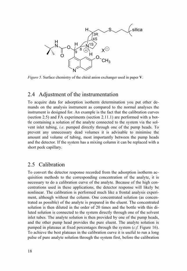
Figure 5. Surface chemistry of the chiral anion exchanger used in paper V.

2.4 Adjustment of the instrumentation To acquire data for adsorption isotherm determination you put other de-mands on the analysis instrument as compared to the normal analyses the instrument is designed for. An example is the fact that the calibration curves (section 2.5) and FA experiments (section 2.11.1) are performed with a bot-tle containing a solution of the analyte connected to the system via the sol-vent inlet tubing, i.e. pumped directly through one of the pump heads. To prevent any unnecessary dead volumes it is advisable to minimise the amount and volume of tubing, most importantly between the pump heads and the detector. If the system has a mixing column it can be replaced with a short peek capillary.

2.5 Calibration To convert the detector response recorded from the adsorption isotherm ac-quisition methods to the corresponding concentration of the analyte, it is necessary to do a calibration curve of the analyte. Because of the high con-centrations used in these applications, the detector response will likely be nonlinear. The calibration is performed much like a frontal analysis experi-ment, although without the column. One concentrated solution (as concen-trated as possible) of the analyte is prepared in the eluent. The concentrated solution is then diluted in the order of 20 times and the bottle with this di-luted solution is connected to the system directly through one of the solvent inlet tubes. The analyte solution is then provided by one of the pump heads, and the other pump head provides the pure eluent. The analyte solution is pumped in plateaus at fixed percentages through the system (c.f. Figure 16). To achieve the best plateaus in the calibration curve it is useful to run a long pulse of pure analyte solution through the system first, before the calibration

19

curve is started. When the calibration curve from the diluted solution is fin-ished, the same procedure is repeated with the concentrated solution that was prepared first, to cover the whole concentration range of the adsorption iso-therm. If it is possible, the option of using UV/Vis spectra is useful when the cali-bration curves are acquired. It is then possible to pick out the best suitable wavelength that stays below saturation of the detector response for the high concentrations, but at the same time has a response high enough to give a good signal for the lowest concentrations. This can be somewhat of a chal-lenge for some analytes. If necessary, different wavelengths can be used for different parts of the calibration curve. Nonetheless, the calibration curve for the high concentrations will most likely be strongly nonlinear.

2.6 Injection profiles One important input parameter in the use of numerical optimisation software is the injection profile [15]. In analytical applications the injection profile is usually of minor importance, unless it is very wide or tailing to a great ex-tent. The bandwidth of the injection profile is, in analytical cases, usually very small compared to the bandwidth of the eluted peak. It is however of greater importance in preparative chromatography, when large volumes are injected [18] and the retention time is low. Studies of commercial injector and detector systems through direct connec-tion of the injector to the detector cell has shown that many systems exhibit remarkably high extra-column dispersion from the injection, in relation to the columns they are designed for [19]. When it comes to compounds with little or no retention this dispersion becomes critical, because more than 80% of the band broadening can arise from extra-column dispersion [20], a re-markable observation considering that process systems often are adjusted for low retention.

20

Figure 6. Experimental illustration from paper I of the flow effect on (a) 5 µL injec-tion profiles, (b) 50 µL injection profiles and (c) 200 µL injection profiles of 1 mM 3-phenyl-1-propanol (PP) in a 45% MeOH solution. See legend for flow explana-tions.

The injection profile is often represented by a rectangular pulse in the opti-misation software [21-23] but can also be represented by a number of differ-ent theoretical profiles, such as Danckwert’s boundary conditions [21,24,25], one half of a Gaussian function [26], a quasi-Gaussian function (two half Gaussian profiles with slightly different standard deviations) [27] and the Exponentially Modified Gaussian (EMG) function [28,29]. The EMG func-tion has also been used for characterisation of asymmetrical eluted peaks [30,31]. However, it has been known for some time that better agreements between calculated and experimental eluted profiles usually are achieved if the real experimental injection profiles are used [26,32]. This has been spe-cifically demonstrated for the IM in some recent publications [28,29,33]. It was also shown recently that in adsorption isotherm determinations using the ECP method, the injection profile may introduce a serious error in the iso-

21

therm data. A new injection method was developed to more or less eliminate these effects [34]. The issue of the injection profile has remained largely un-investigated for the last 20 years. This is remarkable since the importance of accounting for the experimental injection profiles was demonstrated in an early theoretical pa-per [26]. A systematical and fundamental investigation on how the shape of the injection profile varies with a number of experimental conditions was therefore desirable (Paper I).

Figure 7. Injection profiles from paper I displaying the effect of (a) different mo-lecular mass of the solute (Bovine Serum Albumin > Green Fluorescent Protein >> Phenol) and (b) phenol injections with different viscosity of the eluent (45% metha-nol > 100% Water > 100% Methanol). All injections were 400 µL.

An experimental investigation was done on how the shape of the injection profile depends on different injection volumes, inner diameters of the loop capillary, flow rates, eluent compositions and molecule masses of the sol-utes. This was done by connecting the detector cell directly to the autosam-pler injection valve on an Agilent 1200 system, using the capillaries and pre-column filter normally used, but without the column. The shape of the injec-tion profile arises during the propagation of the solute zone through the loop and the capillaries, which are open cylindrical tubes of small bore. The ex-

22

periments revealed that the injection profile becomes more dispersed with increased flow rate and injection volume (Figure 6), increased molecular mass of the solute and viscosity of the eluent (Figure 7), and increased inner diameter of the injection loop capillary (Figure 8). An inner diameter of 1.0 mm gives a long dispersed tail. The dispersion dramatically decreases when the inner diameter is decreased by half to 0.5 mm, and even more when the diameter is decreased further, to 0.25 mm. The smaller the inner diameter, the lower the influence of the parabolic flow profile on the dispersion of the tail.

Figure 8. Experimental illustration from paper I of the effect of the inner diameter of the loop on the injection profile. 200 µL injections of PP.

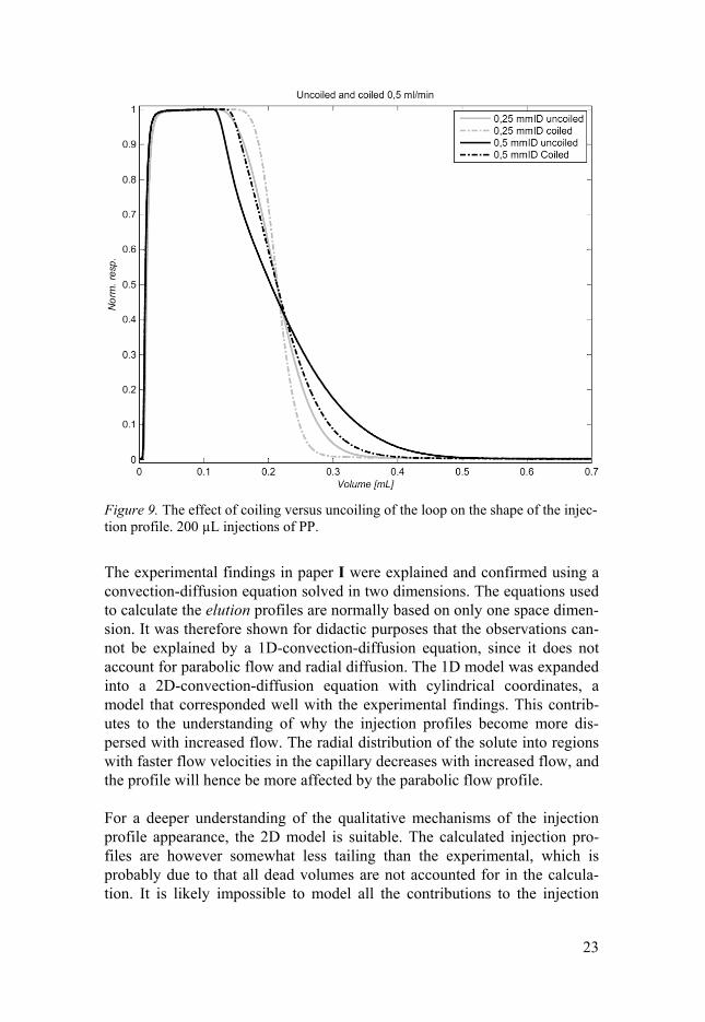
The coiling of the loop also has an influence on the shape of the injection profile. As can be seen in Figure 9, a coiled loop (diameter 4.2 cm) gives a clearly less tailing profile than an uncoiled loop. This can be ascribed to the effect that the centripetal forces has on the flow profile, reducing the para-bolic flow to a more flat flow profile.

23

Figure 9. The effect of coiling versus uncoiling of the loop on the shape of the injec-tion profile. 200 µL injections of PP.

The experimental findings in paper I were explained and confirmed using a convection-diffusion equation solved in two dimensions. The equations used to calculate the elution profiles are normally based on only one space dimen-sion. It was therefore shown for didactic purposes that the observations can-not be explained by a 1D-convection-diffusion equation, since it does not account for parabolic flow and radial diffusion. The 1D model was expanded into a 2D-convection-diffusion equation with cylindrical coordinates, a model that corresponded well with the experimental findings. This contrib-utes to the understanding of why the injection profiles become more dis-persed with increased flow. The radial distribution of the solute into regions with faster flow velocities in the capillary decreases with increased flow, and the profile will hence be more affected by the parabolic flow profile. For a deeper understanding of the qualitative mechanisms of the injection profile appearance, the 2D model is suitable. The calculated injection pro-files are however somewhat less tailing than the experimental, which is probably due to that all dead volumes are not accounted for in the calcula-tion. It is likely impossible to model all the contributions to the injection

24

profiles in a real experimental setting; it will always be an estimation. To make the situation even more complicated, all extra contributions from dead volumes will have a flow dependency [35]. The results give useful informa-tion on how to minimise extra-column band broadening effects caused by the injection profile, which in turn can improve the accuracy in the post-processing methods. This is important both for preparative and analytical chromatography; in particular for modern analytical systems using short and narrow columns. In a follow up study (paper II) it was investigated how to predict accurate injection profiles in numerical optimisation of preparative separations, with a minimum of experimental injection profiles required. The model used to predict the profiles was a modified EMG function, i.e. a convolution be-tween a Gaussian pulse and function with an inital constant plateau followed by an exponentially decaying tail. It was found that as little as two experi-mental profiles were enough to predict accurate profiles of other volumes, within one flow. If the flow was to be included in the optimisation, only two more experimental profiles were required.

2.7 Void volume determination It is important for these applications to do a careful determination of the void volume of the column, also called t0. An incorrect determination of the void can lead to misinterpretations in the subsequent processing of the data. It is especially important in characterisation studies [36] but somewhat less im-portant in process optimisation [37]. The determination of t0 can be done with some different approaches, but is normally done by injecting an unre-tained marker on the column. This is however associated with some chal-lenges, with respect to the retention issue. It is difficult to find a marker that is completely unaffected by the stationary phase in all ways, and in all ex-perimental cases. In the case of repulsion in any way between the marker and the stationary phase, the void volume will seem to be smaller than it really is. This could happen for example with the charged void volume marker sodium nitrate (Figure 10a). Even if the marker is unaffected in some conditions; a change in for example pH might change the ionisation state of the marker and/or stationary phase and thus possibly introducing an interac-tion between the two. This is the case with for example uracil (Figure 10b), a common void volume marker, which has a pKa of 9.45 [38]. Uracil and so-dium nitrate were used in paper III, uracil and potassium nitrate (an ana-logue to sodium nitrate but with a potassium ion instead of a sodium ion) were used in paper IV. Another common void volume marker is acetone, which was used in polar organic mode in paper V (Figure 10c).

25

Figure 10. Chemical structures of common void volume markers, a) Sodium nitrate, b) Uracil, c) Acetone.

2.8 pH effects Many compounds that contain basic amino functions can be found e.g. on the pharmaceutical market. Numerous studies on the behaviour of ionisable compounds in RPLC have been conducted throughout the years [39-44], perhaps because the large amount of pharmaceutical substances that belong to this category. The issue of pH when such compounds are analysed with liquid chromatography is a delicate matter. Depending on where along the pH-scale the experiments are performed relative to the pKa of the analyte, the compound can be present in different ratios of charged and uncharged form, which under some circumstances can have a dramatic effect on the chroma-tographic performance. It is reasonable to think that dissolving high concentrations of a protolytic compound in the eluent may lead to pH differences between sample and eluent, which in turn may lead to deviating band shapes when overloading the column [45,46]. It can be crucial to control this possible difference, since severe deformations of the bands can occur if the pH difference is large. The difference can be avoided by considering which protolytic form of the com-pound that should be used. It has been shown in studies of adsorption iso-therms that pH matched and pH mismatched samples will result in different parameters [47]. It has recently been demonstrated, using mathematical models, how peculiar overloaded band profiles of basic compounds are due to the local pH in the column when using low capacity buffers [48]. Paper III is a descriptive study where the experimental conditions cause dramatic changes to the band shapes of ionisable compounds, in the absence of a pH difference. Great care was taken to exactly match the pH of the injected so-lutions with the pH of the eluent. The design and outcome of the study con-tradicts current theories on the cause of the band shapes, and shows that complex band shapes may occur irrespective of the most careful experimen-

26

tal design. Even more detailed guidelines on how to avoid pH differences between sample and eluent is given in a follow up study [49]. There can also be other reasons to why peak deformations may occur, such as large system peaks caused by additives in the mobile phase [50,51]. To further complicate the issue of pH, the addition of organic modifiers to the eluent will change the pKa of the solute and the apparent pH of the eluent (i.e. the pKa of the buffer component). These changes are solute and buffer system dependent. The autoprotolysis constant of different solvents varies greatly. Examples of the autoprotolysis constants at 25°C for the solvents used in this thesis are given below: Water: 2 H2O H3O

+ + OH- 14.0 [52]

Methanol: 2 CH3OH CH3OH2+ + CH3O

- 16.7 [53]

Acetonitrile: 2 CH3CN CH3CNH+ + CH2CN- 32.2 [52] When mixing water and organic solvents, the autoprotolysis constant of the mixture does not follow a linear relationship between the two values of the respective pure solvent. A rule of thumb is however that the pKa of acids increases and the pKa of bases decreases upon addition of modifier to the eluent [39]. These changes can lead to confusing results if the eluent pH with modifier present ( pH) is not properly measured; as shown in Figure 1 in [54]. The pH and pKa values in this context is therefore better described by the pH / p scales (calibrated in aqueous solution and measured with organic modifier present) than the pH / p (calibrated and measured in aqueous solution) scales, since the latter can cause poor retention predic-tions.

27

Figure 11. Analytical retention factors versus from paper III for (a) the Kro-masil Eternity column and (b) the PLRP-S column. ME is the solid black line with open circle symbols, BT is the gray solid line with open rectangular symbols, and PP is the black dashed line with open triangular symbols. Note that the retention of BT increases on both columns, and the drastic drop of ME at high on the PLRP-S column. See the structures of the solutes in Figure 2.

The first part of the study is an analytical investigation of the retention factor at different pH for three chosen probes: the basic protolytic compound metoprolol (ME), the constantly positively charged quaternary ammonium ion benzyltriethylammonium chloride (BT), and the neutral compound 3-phenyl-1-propanol (PP). They were studied with analytical injections in 1 pH-unit steps from pH 3 to pH 11. The results are shown in Figure 11. The results follow what was expected, except for two observations. First, why the retention of BT increases at high pH on the polymeric column can-not be explained in the same way as for the silica column [55], since the polymeric surface lack residual silanols. However, there seems to be other negatively charged synthesis residues capable of electrostatic interactions on the polymeric phase [5,6]. Second, the drastic decrease in retention factor of ME at high pH on the polymeric column can be a cease in the strong cation exchange mechanism when the solute becomes uncharged [6].

28

Figure 12. Overloaded injections of 5, 10 and 20 mM metoprolol (Figure 2a) on four different reversed phase columns. All columns have C18 surface chemistry except for the Shodex ODP2 HP-4D column in the lower right panel, which is purely polymeric.

The main focus of the study was however on an expanded investigation in-spired by previously observed distorted overloaded band shapes at interme-diate pH (see Figure 12), i.e. type II isotherm bands (see Figure 15) of the basic probe metoprolol. This type of band shape around the pKa of ionisable compounds (pKa for metoprolol is approximately 9.60-9.70 [56,57]) has been noticed previously [43,48,54,58,59]. The change in shape of the band in this interval, indicating a switch of the adsorption isotherm type, is sug-gested to appear when the solute concentration is high enough to cause local pH differences between the sample and the eluent [43,48,59]. The overloaded study was performed in steps of 1 pH-unit covering the p of the base, to reveal in more detail where the deformed bands occur. Results from the silica C18 column are shown in Figure 13, where 5, 10 and 20 mM injections of metoprolol in 20 mM pH phosphate buffer with MeOH are shown. The column was Eternity C18, a recently released organic hybrid silica C18 column with ethyl groups inserted as an organic/inorganic interfacial gradient from the surface and down. Despite the fact that the in-jected solutions containing the base are very carefully pH-matched with the eluent, the deformed peaks still occur. In this case, the deformation cannot be explained by an initial pH difference. However, in a study of an ion-selective electrode, it was suggested that a local pH gradient on the surface occurs [60], which could be possible also on a silica surface. The relation to the pKa (i.e. the ionisation state) of the solute seems clear however, judging from where in the pH interval the distorted peaks occur.

29

Another result from the study is that this distortion effect does not appear on polymeric columns without C18 ligands in the concentration range studied. It only appears on columns with C18 ligands, independently of the base ma-trix (silica, hybrid silica or polymeric). The purely polymeric phase (PLRP-S) used in the present work shows an increase in analytical retention time at intermediate to high pH for a positively charged quaternary amine, to an even greater extent than on the silica C18 column. This suggests that there are negative groups [6] also on the polymeric phase, similar to residual si-lanols on silica columns, which are often blamed for poor performance. The phenomenon of the distorted peaks is however not observed on the poly-meric phase without C18 chains (for these results, see Paper III). The constantly positively charged quaternary ammonium ion BT, and the neutral compound PP, were also accordingly overloaded on both columns, but showed no deviating behaviour (see Paper III).

30

Figure 13. Overloaded injections from paper III, of 5, 10 and 20 mM metoprolol (Figure 2a) in eluent-sample pH-matched solutions on the silica C18 column. Note the drastic change in the shape of the bands.

2.9 Temperature effects It is well known that the temperature has a large effect on the performance of chromatographic systems [61]. When doing adsorption studies it is important to maintain a constant temperature on the column. This can be done by using an air temperature controlled column compartment as a part of the instru-ment stack. It is however easier to maintain a constant temperature by using a temperature controlled circulating water bath. This approach was used in all elution experiments in the papers included in this thesis.

31

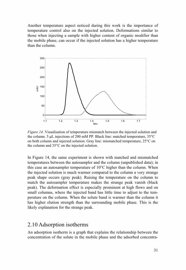
Another temperature aspect noticed during this work is the importance of temperature control also on the injected solution. Deformations similar to those when injecting a sample with higher content of organic modifier than the mobile phase, can occur if the injected solution has a higher temperature than the column.

Figure 14. Visualisation of temperature mismatch between the injected solution and the column. 5 μL injections of 200 mM PP. Black line: matched temperature, 35°C on both column and injected solution. Gray line: mismatched temperature, 25°C on the column and 35°C on the injected solution.

In Figure 14, the same experiment is shown with matched and mismatched temperatures between the autosampler and the column (unpublished data); in this case an autosampler temperature of 10°C higher than the column. When the injected solution is much warmer compared to the column a very strange peak shape occurs (gray peak). Raising the temperature on the column to match the autosampler temperature makes the strange peak vanish (black peak). The deformation effect is especially prominent at high flows and on small columns, where the injected band has little time to adjust to the tem-perature on the column. When the solute band is warmer than the column it has higher elution strength than the surrounding mobile phase. This is the likely explanation for the strange peak.

2.10 Adsorption isotherms An adsorption isotherm is a graph that explains the relationship between the concentration of the solute in the mobile phase and the adsorbed concentra-

1.1 1.2 1.3 1.4 1.5 1.6 1.7

0

50

100

150

200

250

300

Min

mAU

32

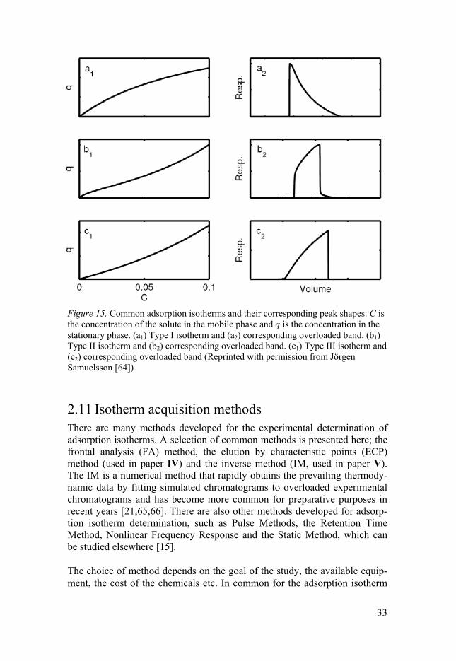
tion in the stationary phase, under specific and constant temperature condi-tion [15]. The most common adsorption isotherms and their corresponding peak shapes are shown in Figure 15. When it comes to linear chromatogra-phy, it revolves around the very initial slope of the apparent isotherm, and is unable to, for one specific analyte, distinguish individually between possibly different adsorption sites. It is thus not capable of explaining the complete retention mechanisms in one go; i.e. the effects and the consequences in the case of a heterogeneous surface. In order to give a complete picture of the retention mechanism, isotherms over a very wide range of concentrations (as wide as possible) are required [7]. When the concentration of the samples becomes very high, some special experimental considerations and pitfalls that rarely are encountered in other applications are introduced. Examples of such pitfalls are solubility prob-lems, changes in viscosity of the sample and issues regarding the buffering capacity of the liquid that is used to dissolve the sample. Special considera-tions are also introduced regarding the detector, such as linearity and dy-namic range of the detector response. There is almost no exception to the fact that the response factor of the detector needs to be adjusted to obtain a lower than the maximum response for the analyte in these cases (e.g. altering the wavelength on a UV detector), to avoid saturation of the detector signal. It might be necessary to use different wavelengths for different parts of the isotherm (see chapter 2.5 on calibration). Depending on the mechanisms of the adsorption of the compound, the iso-therm can display different curvatures. Different isotherm shapes have been suggested and described for gas-solid equilibriums [62,63], but these can also be encountered in liquid-solid equilibrium applications. The most com-mon isotherm shape is the type I isotherm, which is convex and eventually reaches a saturation level (qs). Highly overloaded chromatograms of a solute that exhibits a type I isotherm behaviour (often called Langmuir type iso-therm) will display a right-angled triangular shape with a sharp front and a diffuse rear [15]. Examples of the most common isotherm types and their corresponding overloaded peak shapes are shown in Figure 15. All these peak shapes were observed in Paper III (see Figure 13).

33

Figure 15. Common adsorption isotherms and their corresponding peak shapes. C is the concentration of the solute in the mobile phase and q is the concentration in the stationary phase. (a1) Type I isotherm and (a2) corresponding overloaded band. (b1) Type II isotherm and (b2) corresponding overloaded band. (c1) Type III isotherm and (c2) corresponding overloaded band (Reprinted with permission from Jörgen Samuelsson [64]).

2.11 Isotherm acquisition methods There are many methods developed for the experimental determination of adsorption isotherms. A selection of common methods is presented here; the frontal analysis (FA) method, the elution by characteristic points (ECP) method (used in paper IV) and the inverse method (IM, used in paper V). The IM is a numerical method that rapidly obtains the prevailing thermody-namic data by fitting simulated chromatograms to overloaded experimental chromatograms and has become more common for preparative purposes in recent years [21,65,66]. There are also other methods developed for adsorp-tion isotherm determination, such as Pulse Methods, the Retention Time Method, Nonlinear Frequency Response and the Static Method, which can be studied elsewhere [15]. The choice of method depends on the goal of the study, the available equip-ment, the cost of the chemicals etc. In common for the adsorption isotherm

34

determination methods is that the concentration of the solute should be as high as possible in the solution, to cover as much as possible of the adsorp-tion sites [7]. Using this strategy will provide the biggest picture of the reten-tion mechanisms.

2.11.1 Frontal analysis The FA method is considered as one of the most accepted and accurate methods for determination of adsorption isotherms [7,34,67]. This method can be performed in two different modes, the staircase mode and the single step mode. The staircase mode (Figure 16) is faster and consumes less solute and eluent, but has the drawback of lingering errors, i.e. errors from preced-ing steps will tag along to subsequent steps. The single step method resem-bles the staircase method, but includes a re-equilibration with pure mobile phase after every step, making each step independent of the other steps. This makes the single step method more accurate, but with the drawback of longer time and higher eluent and solute consumption [7]. Both methods are carried out similar to the calibration curve, by preparing a high concentration (close to saturation) solution of the compound in the elu-ent. The lowest concentration used for the adsorption isotherm determination should be low enough to give symmetrical breakthrough curves. If they are not symmetrical the solution should be diluted, about 20 times is often suffi-cient, until they become symmetrical. One head of the binary pump provides the analyte solution and the other pump head provides the pure eluent. The analyte solution is pumped through the column in fixed percentage steps; see Figure 16. The procedure is then repeated with the concentrated solution that was first prepared. The adsorption isotherm is calculated based on the con-centrations of the steps and the breakthrough times of the fronts. It is desirable to have an analytical retention factor (k) around 3-5, to get good data. To prevent any back flow it is good to start the frontal analysis at some low percentage (e.g. 0.1%) from the analyte solution pump, and then take the 0% value from the end of the experiment, after the switch back to the pure eluent. The plateaus can then be corrected afterwards from this value. If UV is the detection method, adjustment of the wavelength might be needed to properly detect the lowest concentrations, i.e. it might be neces-sary to use different wavelengths to determine different parts of the iso-therm.

35

Figure 16. FA in the staircase mode. 5, 10, 20, 30… 100% of the analyte solution is pumped through the column. Note the nonlinearity of the detector response.

2.11.2 Elution by characteristic points The ECP method is an experimentally simple and fast technique based on injection of a large and heavily overloaded pulse (see Figure 17). ECP has been previously studied regarding accuracy [68] and further developed with great success [34]. This further developed ECP method is performed with a so-called cut-injection technique and gives nearly identical adsorption iso-therms as reference methods that are known to be accurate (i.e. FA). The accuracy originates from the generation of nearly rectangular injection pro-files, obtained by turning the injection valve back before the dispersed tail of the injection plug exits the loop [34]. The tail is thus left in the injection loop and never reaches the column. The isotherm is then derived from the rear part of the elution band. The ECP method was used successfully in paper IV. Since then, the method for evaluation of the ECP tail has been even further developed, to the so called ECP-slope method [69], and also expanded to handle other isotherms than type I isotherms [70].

50 100 150 200 250 3000

200

400

600

800

1000

1200

1400

Min

mAU

36

Figure 17. ECP pulse. The adsorption isotherm is determined from the diffuse rear of the pulse.

2.11.3 The inverse method The IM is an “indirect” method of adsorption isotherm determination, which has increased in popularity during recent years. The IM is a fast numerical method that determines the adsorption isotherm parameters by repeatedly fitting simulated band profiles to overloaded experimental profiles, until a good fit is obtained [21,65,66], see Figure 18. In this way, the isotherm pa-rameters are repeatedly “guessed” (indirect method); as opposed to e.g. FA where the actual data points on the adsorption isotherm is obtained (direct method). In addition to the overloaded runs, analytical runs are used to ob-tain a good estimation of the initial slope of the isotherm. This method re-quires much less experimental work to obtain the necessary adsorption data than the more lengthy and demanding FA, however with the drawback of lower accuracy. In paper V, the inverse method was used with good results to develop optimisation strategies for taking an additive into account when optimising preparative separations of a stereoisomeric pair. The IM is an excellent choice of method in this case, as it easily determines isotherm pa-rameters for more than one component simultaneously, as opposed to e.g. FA where that is hard or even impossible.

12 14 16 18 20 22 24 26 28 30

0

500

1000

1500

Min

mAU

37

Figure 18.

Illu

stra

tion

of th

e In

vers

e M

etho

d. (

a) T

he b

lue

prof

ile is

the

expe

rim

enta

l pro

file

. The

red

pro

file

rep

rese

nts

the

ini-

tial g

uess

of

adso

rptio

n is

othe

rm p

aram

eter

s. (

b) T

he s

imul

atio

n is

rep

eate

d un

til th

e ex

peri

men

tal a

nd th

e si

mul

ated

pr

ofile

coi

ncid

e.

38

3. Processing of adsorption data

Presented below is a possible workflow which can be used to process the data from the isotherm acquisition methods. An overview of the workflow is shown in Figure 19. An exception to this workflow is when the IM is used for the determination of the adsorption isotherm, in which case the adsorp-tion model is assumed already prior to the fitting.

Figure 19. Workflow for elucidation of an accurate isotherm model.

3.1 Scatchard plots Once the adsorption isotherm data is acquired, it is time to elucidate what adsorption model that fits the data. A first useful step is to make a scatchard plot, where q/C is plotted against q (where q is the concentration in the sta-tionary phase and C is the concentration in the mobile phase). The curvature of the graph in the scatchard plot will give useful hints about the adsorption model. Displayed in Figure 20 are scatchard plots for isotherm models of type I (see Figure 15). Isotherms with inflection points (e.g. type II iso-therms) will give scatchard plots with a minimum or maximum, or both [7].

39

Figure 20. Scatchard plots representing the Langmuir, bi-Langmuir, Tóth and Jovanovic isotherm models (Reprinted with permission from Jörgen Samuelsson [64]).

3.2 Adsorption energy distribution AED is a novel tool that independently of an adsorption model uses the ex-perimental adsorption isotherm data to qualitatively determine the degree of heterogeneity of the adsorbent [71]. The heterogeneity includes the number of interaction sites, their relative abundance and their energies. Examples of results from AED calculations can be seen in Figure 21, where a one site model (Langmuir, grey line) as well as a two site model (bi-Langmuir, black line) is shown. The number of sites can however be even higher, depending on the experimental system that is studied. The appearance of the AED plot hence gives independent clues to what initial model to assume in the subse-quent fitting of the adsorption isotherm data to an isotherm model, see Sec-tion 3.3.

40

Figure 21. Example of AED for the Langmuir (one site) and the bi-Langmuir (two sites) models. ln K is the natural logarithm of the equilibrium constant and qs is the saturation capacity of the stationary phase (Reprinted with permission from Jörgen Samuelsson [64]).

3.3 Fitting of experimental data to an isotherm model When two or more likely adsorption isotherm models are chosen based on previous steps, the next step is to fit the experimental adsorption data to these models. This is usually done with a non-linear regression analysis, using a method that minimises the residual sum of squares of the relative difference between the calculated model based data and the experimental data. A statistical value called the Fisher parameter is calculated for each isotherm model, and a comparison of the Fisher parameters indicates what model that fits the data best. From this fitting, more accurate values of the equilibrium constant (ln K) and the saturation capacity (qs) are obtained, as compared to the values obtained from the AED. An example of what the fitting can look like is shown in Figure 22.

41

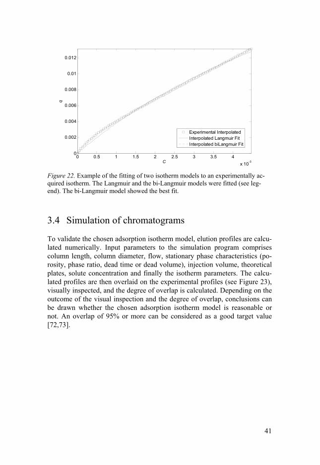
Figure 22. Example of the fitting of two isotherm models to an experimentally ac-quired isotherm. The Langmuir and the bi-Langmuir models were fitted (see leg-end). The bi-Langmuir model showed the best fit.

3.4 Simulation of chromatograms

To validate the chosen adsorption isotherm model, elution profiles are calcu-lated numerically. Input parameters to the simulation program comprises column length, column diameter, flow, stationary phase characteristics (po-rosity, phase ratio, dead time or dead volume), injection volume, theoretical plates, solute concentration and finally the isotherm parameters. The calcu-lated profiles are then overlaid on the experimental profiles (see Figure 23), visually inspected, and the degree of overlap is calculated. Depending on the outcome of the visual inspection and the degree of overlap, conclusions can be drawn whether the chosen adsorption isotherm model is reasonable or not. An overlap of 95% or more can be considered as a good target value [72,73].

0 0.5 1 1.5 2 2.5 3 3.5 4x 10-3

0

0.002

0.004

0.006

0.008

0.01

0.012

C

q

Experimental InterpolatedInterpolated Langmuir FitInterpolated biLangmuir Fit

42

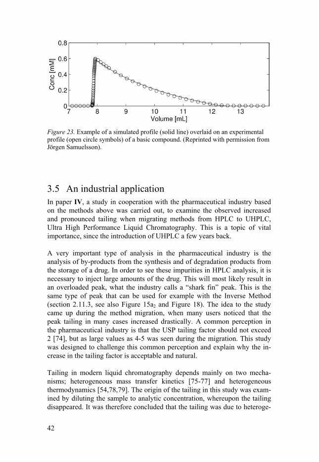
Figure 23. Example of a simulated profile (solid line) overlaid on an experimental profile (open circle symbols) of a basic compound. (Reprinted with permission from Jörgen Samuelsson).

3.5 An industrial application In paper IV, a study in cooperation with the pharmaceutical industry based on the methods above was carried out, to examine the observed increased and pronounced tailing when migrating methods from HPLC to UHPLC, Ultra High Performance Liquid Chromatography. This is a topic of vital importance, since the introduction of UHPLC a few years back. A very important type of analysis in the pharmaceutical industry is the analysis of by-products from the synthesis and of degradation products from the storage of a drug. In order to see these impurities in HPLC analysis, it is necessary to inject large amounts of the drug. This will most likely result in an overloaded peak, what the industry calls a “shark fin” peak. This is the same type of peak that can be used for example with the Inverse Method (section 2.11.3, see also Figure 15a2 and Figure 18). The idea to the study came up during the method migration, when many users noticed that the peak tailing in many cases increased drastically. A common perception in the pharmaceutical industry is that the USP tailing factor should not exceed 2 [74], but as large values as 4-5 was seen during the migration. This study was designed to challenge this common perception and explain why the in-crease in the tailing factor is acceptable and natural. Tailing in modern liquid chromatography depends mainly on two mecha-nisms; heterogeneous mass transfer kinetics [75-77] and heterogeneous thermodynamics [54,78,79]. The origin of the tailing in this study was exam-ined by diluting the sample to analytic concentration, whereupon the tailing disappeared. It was therefore concluded that the tailing was due to heteroge-

43

neous thermodynamics and not due to heterogeneous mass transfer kinetics, in which case the tailing would have persisted. The method used for isotherm determination in paper IV was the ECP method with cut-injection technique [34], described in section 2.11.2. The model substance was the basic drug metoprolol (a beta blocker, see Figure 2a). The scatchard plots were concave; the AEDs indicated a two site model and the best fitting isotherm was found to be the bi-Langmuir isotherm.

44

4. Optimisation of preparative separations

In large scale industrial separation and purification processes there are re-quirements for optimisation with regards to several different parameters. Some parameters that are generally optimised include injected amount/feed, mobile phase velocity and mobile phase composition [15]. The goal in most cases is the maximum productivity at a certain required yield and purity. This can be achieved empirically by conducting experiments under numer-ous different conditions and then trying to pick the conditions that give the best results. The empirical approach can however be very time- and labour consuming, especially if it has to be done often and in large scale, e.g. in the case of simulated moving bed, SMB. An alternative approach to process optimisation is to utilise computing power and optimisation algorithms, in order to find the best experimental parameters numerically. This procedure also requires some manual experi-mental laboratory work, but not near the extent of the laboratory work needed for empirical optimisation. It depends however on how many vari-ables that are to be optimised. In case of just one, e.g. injection volume, it can save time to avoid numerical optimisation. If more than one variable, numerical optimisation may be favourable. Experiments required for highly accurate numerical optimisations are the van Deemter curves (or equivalent, e.g. Knox curves), injection profiles (see Section 2.1) and elution profiles, at some different conditions. Knowledge about the adsorption isotherm is re-quired [15,67]. For examples of methods for adsorption isotherm determina-tion, see Section 2.11. Different approaches can be used for the optimisation. A common approach is to have a function that depends on a number of different parameters (such as productivity, depending on flow, injected volume etc.). Some of the pa-rameters are kept constant and the optimisation is performed for the non-constant parameters. A common strategy is to set all the parameters as con-stant except for the injection volume, and then optimise this volume in com-bination with the fixed parameters. This is called “sub-optimisation”. This is; in a sense; the same approach that is used for empirical optimisation, but in the empirical case it is performed experimentally, not numerically.

45

Another optimisation strategy is a more extensive approach using TOMLAB [80], that can handle “costly” optimisation problems. The function is calcu-lated for a number of points from which a response surface is interpolated. The optimisation is then performed over this surface. It is done iteratively, i.e. the function is subsequently calculated for the found optimal value and compared to the interpolated surface value. If it differs, the function is calcu-lated for additional points and a new response surface is interpolated, over which the optimisation is performed. Several optimisation strategies were investigated and compared in paper V, with the primary aim of highlighting the importance of the additive choice and to properly account for the additive in optimisation methods. Three op-timisation methods were compared; injection volume optimisation, injection volume and additive concentration optimisation, and full optimisation in-cluding injection volume, additive concentration, sample concentration and flow rate. In the last case the TOMLAB approach (described above) was used, and gave the overall best results. If the additive is included in the ad-sorption model and in the numerical optimisation, it is possible both to in-crease the production rate and to choose the additive that is most beneficial for the separation.

46

5. Concluding remarks and future aspects

The studies of adsorption mechanisms can provide a deeper understanding and knowledge about fundamental events in liquid chromatography. The main application for the studies in this thesis is nonlinear and preparative chromatography, but the results also contribute to the overall understanding of chromatography. To start with, two studies of the band broadening events occurring outside the column, i.e. the so-called injection profile, were conducted. The aim of the first one (paper I) was to deduce if and how a set of experimental pa-rameters affect the spreading of a band. With the results in mind, action can be taken to decrease band spreading contributions from extra-column sources, to improve the chromatographic performance. The second one (pa-per II) had the main purpose to find an approach to reduce the amount of experimental injection profiles required to a minimum, and still be able to perform highly accurate process optimisations. As a follow up study to a previous paper from the group, a study of pH and the performance of protolytic compounds (in this case a base) was conducted (Paper III). It was found that despite the most careful experimental design to avoid pH differences, severe deformations of the bands may still occur. The deformations seem under the prevailing conditions to be dependent on what separation system is used and proves that deviating peak shapes can appear no matter how much effort is made to avoid pH differences. Paper IV used the methods mentioned in this thesis to demonstrate that the common perception that the USP tailing factor should be <2 is no longer valid when the highly efficient separation systems of today are used. UHPLC produces noticeably higher tailing factors than the predecessor HPLC, but still with a better resolution to adjacent peaks. In paper V, different optimisation strategies were examined, with the aim to properly account for the type and concentration of the additive in chiral preparative chromatography. It was found that it was not only possible to increase the production rate, but also to choose the additive that is most fa-vourable for the separation at hand.

47

The overall goal of these studies is to gain a better understanding of, and to improve the performance of, preparative chromatographic processes. With an in-depth knowledge about the properties and the behaviour of the system, the chances of a fast and effective process increases. This in turn makes it possible to produce e.g. highly purified APIs to a reduced cost. The methods for characterisation and optimisation of separation processes can undoubtedly be further developed and improved, as well as applied for different separation methods in addition to HPLC. A wish for the future could be to have easily accessible and user friendly software to handle these types of computer assisted challenges. This way, computer assisted tools for improvement of separation and purification processes might be more ac-cepted and embraced by disciplines outside the academia.

48

6. Acknowledgement

There are a number of people I want to thank for who and where I am today:

Initially, I owe my courage to embark on the chemistry path in the first place to one specific person: Barbro Schröder, my chemistry teacher from Kat-edralskolan. Thank you for your firm encouragement when I asked you if chemistry was something for me!

My advisors Jonas Bergquist and Torgny Fornstedt, for giving me the opportunity to embark on this scientific journey. My co-advisors Per Sjöberg, Titti Ekegren and Jan Carlsson for the help, input and feedback, whether scientific or non-scientific, on whatever was on my mind.

My co-authors Jörgen Samuelsson and Patrik Forssén, for their patient guidance and their contributions to the papers. Torgny Undin and Martin Enmark, for great company in the separation science group. All other co-authors, for good cooperation and for their contributions to the papers.

All past and present roommates and colleagues at Kemi - BMC, for con-tributing to my scientific and social skills in so many ways. Extra thanks to Ulla, Barbro, Fredrika, Eva, Yngve, Erik and Bosse for all help with eve-rything beside the research. A special shimmering star to Anne-Li, Julia and Torgny, for all the support and pep talk during the final ascent!

My teaching colleagues at Analytisk Farmaceutisk Kemi, especially Anita, Annica, Jacob and Victoria. It was educative times!

All my fantastic friends, for being there whenever a friend is needed. You know who you are!

My parents Rolf and Monika, for their unprejudiced and endless love and support, for encouraging me to be independent and to pursue my own goals.

My sister Annika and her family Olle, Rebecka, Valter and Jonatan, for being so generous and loving no matter when.

My family David, Malva and Tuva, for being absolutely adorable. Thank you for filling my life with other things than work! ♥

Thank you all!

49

7. Summary in Swedish

Adsorptionsstudier med vätskekromatografi

Experimentella beaktanden för grundlig bestämning av adsorptionsdata Kromatografi är en metod som enligt IUPAC definieras som ”En fysisk me-tod för separation i vilken komponenterna som ska separeras distribueras mellan två faser, en som är fast (den stationära fasen) medan den andra (den mobila fasen) rör sig i en bestämd riktning” [1]. De första kromatografiska metoderna beskrevs av den ryska vetenskapsmannen Michael Tswett i början av 1900-talet, då han i ett föredrag berättade hur han separerat plantpigment lösta i petroleumeter med ”swedish paper” som stationär fas [2]. Så föddes den första kromatografiska separationstekniken!

Figur 24. Schematisk bild över komponenterna som ingår i ett vätskekromatogra-fiskt separationssystem.

I Reversed Phase, som är det separationssätt som i huvudsak används i den här avhandlingen, fördelar sig analyterna mellan en polär mobil fas och en opolär stationär fas. Den mobila fasen är oftast en vattenlösning med en viss halt av en organisk modifierare, såsom metanol eller acetonitril, samt en buffert eller någon form av salt. Den stationära fasen packas i rör som kallas kolonner (se ”Kolonn” i Figur 24). Den stationära fasen består ofta av alkyl-kedjor, vanligast är kedjor med 18 kol (C18), fästa på ytan av porösa kisel-

50

partiklar. Den kan även bestå av porösa polymerpartiklar, med eller utan alkylkedjor. Idag är vätskekromatografi (på engelska High Performance Liquid Chroma-tography, HPLC) en etablerad arbetshäst och ett mångsidigt verktyg i många olika industrier. Det används för identifiering och kvantifiering av intressan-ta ämnen som generellt förekommer i låga koncentrationer, i så kallad analy-tisk skala. Det kan även användas för att rena fram och isolera värdefulla ämnen som förekommer i höga koncentrationer, så kallad preparativ kroma-tografi. Med höga koncentrationer kan man även ta fram något som kallas för adsorptionsisotermer (se Figur 25).

Figur 25. Vanliga adsorptionsisotermer och deras motsvarande överladdade topp-former. C är koncentrationen av substansen i den mobila fasen och q är koncentra-tionen i stationära fasen. (a1) Typ I-isotherm och (a2) korresponderande överladdad topp. (b1) Typ II-isotherm och (b2) korresponderande överladdad topp. (c1) Typ III-isotherm and (c2) korresponderande överladdad topp (Reproducerad med tillåtelse från Jörgen Samuelsson [64]).

Adsorptionsisotermer är ett värdefullt redskap av många anledningar. De kan användas för karakterisering av kromatografiska separationssystem, och ger då information om retentionsmekanismen samt möjligheten att studera re-producerbarheten mellan kolonner och mellan batcher. Om ett protein im-mobiliseras på ett fast underlag kan man använda adsorptionsisotermer för

51

farmakologisk karakterisering av interaktioner mellan läkemedel och prote-in. Dessutom kan de användas för att studera märkliga kromatografiska fe-nomen. Om man känner till adsorptionsisotermen är det därtill möjligt att simulera kromatogram, och därefter optimera separationsprocessen med datorkraft. Fördelen med en datoroptimerad separationsprocess är högre renhet eller utbyte av värdefulla ämnen såsom läkemedel eller antioxidanter, samtidigt som man reducerar användningen av lösningsmedel. Sammantaget sparar man tid, pengar och miljöpåverkan. Processen för att ta fram adsorptionsisotermer kräver emellertid ett antal noggranna experimentella överväganden och förberedelser, vilka utgör hu-vudfokus i denna avhandling. Viktiga steg längs vägen omfattar val av sepa-rationssystem och lämpliga analyter, beredning av mobila faser och provlös-ningar, kalibrering, framtagande av injektionsprofiler och kolonnens dödtid samt givetvis själva metoden för bestämningen av adsorptionsisotermen. Det är även viktigt att hålla ordning på parametrar som temperatur och pH. Dessa frågor behandlas i denna avhandling. På slutet presenteras en genomgång av användbara metoder för bearbetning av rådata från bestämningen av adsorptionsisotermer, samt en kort beskriv-ning av metoder för optimering med hjälp av datorer.

52

References

[1] A.D. McNaught, A. Wilkinson, IUPAC Compendium of Chemical Terminology. The Gold Book, 2nd Edition, Black-well Science, 1997.

[2] K. Sakodynskii, Journal of Chromatography A 73 (1972) 303. [3] J. Nawrocki, Journal of Chromatography A 779 (1997) 29. [4] U.D. Neue, HPLC columns : theory, technology, and practice,

Wiley-VCH, New York, 1997. [5] S.M.C. Buckenmaier, D.V. McCalley, M.R. Euerby, Analyti-

cal Chemistry 74 (2002) 4672. [6] R. Ruiz, J. Ruiz-Angel, C. Garcia-Alvarez-Coque, C. Rafols,

M. Roses, E. Bosch, Journal of Chromatography A 1028 (2004) 139.

[7] F. Gritti, G. Guiochon, Journal of Chromatography A 1099 (2005) 1.

[8] A. Tchapla, H. Colin, G. Guiochon, Analytical Chemistry 56 (1984) 621.

[9] A. Tchapla, S. Heron, H. Colin, G. Guiochon, Analytical Chemistry 60 (1988) 1443.

[10] K.A. Dill, Journal of Physical Chemistry 91 (1987) 1980. [11] J.G. Dorsey, K.A. Dill, Chemical Reviews 89 (1989) 331. [12] H. Engelhardt, M. Jungheim, Chromatographia 29 (1990) 59. [13] K. Kimata, K. Iwaguchi, S. Onishi, K. Jinno, R. Eksteen, K.

Hosoya, M. Araki, N. Tanaka, Journal of Chromatographic Science 27 (1989) 721.

[14] H.A. Claessens, M.A. van Straten, C.A. Cramers, M. Jezier-ska, B. Buszewski, Journal of Chromatography A 826 (1998) 135.

[15] G. Guiochon, A. Felinger, D.G. Shirazi, A.M. Katti, Funda-mentals of preparative and nonlinear chromatography, 2nd edi-tion, Elsevier Academic Press, Amsterdam, 2006.

[16] F.J. Arnaiz, Journal of Chemical Education 72 (1995) 1139. [17] B.S. Broyles, R.A. Shalliker, D.E. Cherrak, G. Guiochon,

Journal of Chromatography A 822 (1998) 173.

53

[18] G. Guiochon, Journal of Chromatography A 965 (2002) 129. [19] K.W. Freebairn, J.H. Knox, Chromatographia 19 (1984) 37. [20] F. Gritti, A. Felinger, G. Guiochon, Journal of Chromatogra-

phy A 1136 (2006) 57. [21] A. Felinger, A. Cavazzini, G. Guiochon, Journal of Chroma-

tography A 986 (2003) 207. [22] A. Felinger, G. Guiochon, Journal of Chromatography A 752

(1996) 31. [23] A. Felinger, G. Guiochon, Journal of Chromatography A 796

(1998) 59. [24] F. Gritti, G. Guiochon, Journal of Chromatography A 1043

(2004) 159. [25] F. Gritti, G. Guiochon, Journal of Chromatography A 1069

(2005) 31. [26] A.M. Katti, M. Czok, G. Guiochon, Journal of Chromatogra-

phy 556 (1991) 205. [27] F. James, M. Sepulveda, F. Charton, I. Quinones, G. Guio-

chon, Chemical Engineering Science 54 (1999) 1677. [28] A. Felinger, D.M. Zhou, G. Guiochon, Journal of Chromatog-

raphy A 1005 (2003) 35. [29] A. Felinger, F. Gritti, G. Guiochon, Journal of Chromatogra-

phy A 1024 (2004) 21. [30] A. Felinger, Analytical Chemistry 66 (1994) 3066. [31] P.J. Naish, S. Hartwell, Chromatographia 26 (1988) 285. [32] I. Quinones, J.A. Ford, G. Guiochon, Analytical Chemistry 72

(2000) 1495. [33] R. Arnell, P. Forssén, T. Fornstedt, Journal of Chromatography

A 1099 (2005) 167. [34] J. Samuelsson, T. Fornstedt, Analytical Chemistry 80 (2008)

7887. [35] K.P. Hupe, R.J. Jonker, G. Rozing, Journal of Chromatography

285 (1984) 253. [36] J. Samuelsson, P. Sajonz, T. Fornstedt, Journal of Chromatog-

raphy A 1189 (2008) 19. [37] J. Samuelsson, J. Zang, A. Murunga, T. Fornstedt, P. Sajonz,

Journal of Chromatography A 1194 (2008) 205. [38] M.J.O. O'Neil, The Merck index. Ed. 14, Merck & Co.,

Whitehouse Station, N. J., 2006. [39] E. Bosch, P. Bou, H. Allemann, M. Roses, Analytical Chemis-

try 68 (1996) 3651.

54

[40] U.D. Neue, C.H. Phoebe, K. Tran, Y.F. Cheng, Z.L. Lu, Jour-nal of Chromatography A 925 (2001) 49.

[41] F. Gritti, G. Guiochon, Journal of Chromatography A 1028 (2004) 197.

[42] U.D. Neue, T.E. Wheat, J.R. Mazzeo, C.B. Mazza, J.Y. Cava-naugh, F. Xia, D.M. Diehl, Journal of Chromatography A 1030 (2004) 123.

[43] F. Gritti, G. Guiochon, Journal of Separation Science 31 (2008) 3657.

[44] D.V. McCalley, Advances in Chromatography, Vol 46 46 (2008) 305.

[45] B. Streel, A. Ceccato, P. Chiap, P. Hubert, J. Crommen, Bio-medical Chromatography 9 (1995) 254.

[46] A. Vailaya, P. Sajonz, S. Sudah, V. Capodanno, R. Helmy, F.D. Antia, Journal of Chromatography A 1079 (2005) 80.

[47] A. Andrzejewska, F. Gritti, G. Guiochon, Journal of Chroma-tography A 1216 (2009) 3992.

[48] F. Gritti, G. Guiochon, Journal of Chromatography A 1216 (2009) 63.

[49] J. Samuelsson, P. Forssén, T. Fornstedt, Journal of Separation Science 36 (2013) 3769.

[50] L.B. Nilsson, D. Westerlund, Analytical Chemistry 57 (1985) 1835.

[51] A. Sokolowski, T. Fornstedt, D. Westerlund, Journal of Liquid Chromatography 10 (1987) 1629.

[52] I.M. Kolthoff, Chantoon.Mk, Journal of Physical Chemistry 72 (1968) 2270.

[53] J.F. Coetzee, G.R. Padmanabhan, Journal of Physical Chemis-try 66 (1962) 1708.

[54] J. Samuelsson, A. Franz, B.J. Stanley, T. Fornstedt, Journal of Chromatography A 1163 (2007) 177.

[55] U.D. Neue, K.V. Tran, A. Mendez, P.W. Carr, Journal of Chromatography A 1063 (2005) 35.

[56] F. Luan, W.P. Ma, H.X. Zhang, X.Y. Zhang, M.C. Liu, Z.D. Hu, B.T. Fan, Pharmaceutical Research 22 (2005) 1454.

[57] M. Shalaeva, J. Kenseth, F. Lombardo, A. Bastinz, Journal of Pharmaceutical Sciences 97 (2008) 2581.

[58] R. LoBrutto, A. Jones, Y.V. Kazakevich, H.M. McNair, Jour-nal of Chromatography A 913 (2001) 173.

[59] F. Gritti, G. Guiochon, Journal of Chromatography A 1216 (2009) 1776.

55

[60] M. Gratzl, F. Rakias, G. Horvai, K. Toth, E. Pungor, Analytica Chimica Acta 102 (1978) 85.

[61] D. Guillarme, S. Heinisch, J.L. Rocca, Journal of Chromatog-raphy A 1052 (2004) 39.

[62] S. Brunauer, L.S. Deming, W.E. Deming, E. Teller, Journal of the American Chemical Society 62 (1940) 1723.

[63] K.S.W. Sing, D.H. Everett, R.A.W. Haul, L. Moscou, R.A. Pierotti, J. Rouquerol, T. Siemieniewska, Pure and Applied Chemistry 57 (1985) 603.

[64] J. Samuelsson, Acta Universitatis Upsaliensis, Uppsala, 2008, p. 69.

[65] R. Arnell, P. Forssén, T. Fornstedt, Analytical Chemistry 79 (2007) 5838.

[66] P. Forssén, R. Arnell, T. Fornstedt, Computers & Chemical Engineering 30 (2006) 1381.

[67] A. Seidel-Morgenstern, Journal of Chromatography A 1037 (2004) 255.

[68] L. Ravald, T. Fornstedt, Journal of Chromatography A 908 (2001) 111.

[69] J. Samuelsson, T. Undin, A. Törncrona, T. Fornstedt, Journal of Chromatography A 1217 (2010) 7215.

[70] J. Samuelsson, T. Undin, T. Fornstedt, Journal of Chromatog-raphy A 1218 (2011) 3737.

[71] T. Fornstedt, Journal of Chromatography A 1217 (2010) 792. [72] J. Lindholm, T. Fornstedt, Journal of Chromatography A 1095

(2005) 50. [73] R. Arnell, P. Forssén, T. Fornstedt, R. Sardella, M. Lämmer-

hofer, W. Lindner, Journal of Chromatography A 1216 (2009) 3480.

[74] J.W. Dolan, LC GC Europe 16 (2003) 610. [75] T. Fornstedt, G.M. Zhong, G. Guiochon, Journal of Chroma-

tography A 741 (1996) 1. [76] T. Fornstedt, G.M. Zhong, G. Guiochon, Journal of Chroma-

tography A 742 (1996) 55. [77] G. Götmar, T. Fornstedt, G. Guiochon, Journal of Chromatog-

raphy A 831 (1999) 17. [78] J. Samuelsson, T. Fornstedt, Journal of Chromatography A

1203 (2008) 177. [79] G. Götmar, J. Samuelsson, A. Karlsson, T. Fornstedt, Journal

of Chromatography A 1156 (2007) 3.

56

[80] M. Björkman, K. Holmström, Optimization and Engineering 1 (2000) 373.

Acta Universitatis UpsaliensisDigital Comprehensive Summaries of Uppsala Dissertationsfrom the Faculty of Science and Technology 1118

Editor: The Dean of the Faculty of Science and Technology

A doctoral dissertation from the Faculty of Science andTechnology, Uppsala University, is usually a summary of anumber of papers. A few copies of the complete dissertationare kept at major Swedish research libraries, while thesummary alone is distributed internationally throughthe series Digital Comprehensive Summaries of UppsalaDissertations from the Faculty of Science and Technology.(Prior to January, 2005, the series was published under thetitle “Comprehensive Summaries of Uppsala Dissertationsfrom the Faculty of Science and Technology”.)

Distribution: publications.uu.seurn:nbn:se:uu:diva-216235

ACTAUNIVERSITATIS

UPSALIENSISUPPSALA

2014