ADS Load Pull DesignGuide -...

Advanced Design System 2011.01 - ADS Load Pull DesignGuide

1

Advanced Design System 2011.01

Feburary 2011ADS Load Pull DesignGuide


2

© Agilent Technologies, Inc. 2000-20115301 Stevens Creek Blvd., Santa Clara, CA 95052 USANo part of this documentation may be reproduced in any form or by any means (includingelectronic storage and retrieval or translation into a foreign language) without prioragreement and written consent from Agilent Technologies, Inc. as governed by UnitedStates and international copyright laws.

AcknowledgmentsMentor Graphics is a trademark of Mentor Graphics Corporation in the U.S. and othercountries. Mentor products and processes are registered trademarks of Mentor GraphicsCorporation. * Calibre is a trademark of Mentor Graphics Corporation in the US and othercountries. "Microsoft®, Windows®, MS Windows®, Windows NT®, Windows 2000® andWindows Internet Explorer® are U.S. registered trademarks of Microsoft Corporation.Pentium® is a U.S. registered trademark of Intel Corporation. PostScript® and Acrobat®are trademarks of Adobe Systems Incorporated. UNIX® is a registered trademark of theOpen Group. Oracle and Java and registered trademarks of Oracle and/or its affiliates.Other names may be trademarks of their respective owners. SystemC® is a registeredtrademark of Open SystemC Initiative, Inc. in the United States and other countries and isused with permission. MATLAB® is a U.S. registered trademark of The Math Works, Inc..HiSIM2 source code, and all copyrights, trade secrets or other intellectual property rightsin and to the source code in its entirety, is owned by Hiroshima University and STARC.FLEXlm is a trademark of Globetrotter Software, Incorporated. Layout Boolean Engine byKlaas Holwerda, v1.7 http://www.xs4all.nl/~kholwerd/bool.html . FreeType Project,Copyright (c) 1996-1999 by David Turner, Robert Wilhelm, and Werner Lemberg.QuestAgent search engine (c) 2000-2002, JObjects. Motif is a trademark of the OpenSoftware Foundation. Netscape is a trademark of Netscape Communications Corporation.Netscape Portable Runtime (NSPR), Copyright (c) 1998-2003 The Mozilla Organization. Acopy of the Mozilla Public License is at http://www.mozilla.org/MPL/ . FFTW, The FastestFourier Transform in the West, Copyright (c) 1997-1999 Massachusetts Institute ofTechnology. All rights reserved.

The following third-party libraries are used by the NlogN Momentum solver:

"This program includes Metis 4.0, Copyright © 1998, Regents of the University ofMinnesota", http://www.cs.umn.edu/~metis , METIS was written by George Karypis([email protected]).

Intel@ Math Kernel Library, http://www.intel.com/software/products/mkl

SuperLU_MT version 2.0 - Copyright © 2003, The Regents of the University of California,through Lawrence Berkeley National Laboratory (subject to receipt of any requiredapprovals from U.S. Dept. of Energy). All rights reserved. SuperLU Disclaimer: THISSOFTWARE IS PROVIDED BY THE COPYRIGHT HOLDERS AND CONTRIBUTORS "AS IS"AND ANY EXPRESS OR IMPLIED WARRANTIES, INCLUDING, BUT NOT LIMITED TO, THEIMPLIED WARRANTIES OF MERCHANTABILITY AND FITNESS FOR A PARTICULAR PURPOSEARE DISCLAIMED. IN NO EVENT SHALL THE COPYRIGHT OWNER OR CONTRIBUTORS BELIABLE FOR ANY DIRECT, INDIRECT, INCIDENTAL, SPECIAL, EXEMPLARY, ORCONSEQUENTIAL DAMAGES (INCLUDING, BUT NOT LIMITED TO, PROCUREMENT OF

http://www.xs4all.nl/~kholwerd/bool.html

http://www.xs4all.nl/~kholwerd/bool.html

http://www.mozilla.org/MPL/

http://www.mozilla.org/MPL/

http://www.cs.umn.edu/~metis

http://www.cs.umn.edu/~metis

http://www.intel.com/software/products/mkl

http://www.intel.com/software/products/mkl


3

SUBSTITUTE GOODS OR SERVICES; LOSS OF USE, DATA, OR PROFITS; OR BUSINESSINTERRUPTION) HOWEVER CAUSED AND ON ANY THEORY OF LIABILITY, WHETHER INCONTRACT, STRICT LIABILITY, OR TORT (INCLUDING NEGLIGENCE OR OTHERWISE)ARISING IN ANY WAY OUT OF THE USE OF THIS SOFTWARE, EVEN IF ADVISED OF THEPOSSIBILITY OF SUCH DAMAGE.

7-zip - 7-Zip Copyright: Copyright (C) 1999-2009 Igor Pavlov. Licenses for files are:7z.dll: GNU LGPL + unRAR restriction, All other files: GNU LGPL. 7-zip License: This libraryis free software; you can redistribute it and/or modify it under the terms of the GNULesser General Public License as published by the Free Software Foundation; eitherversion 2.1 of the License, or (at your option) any later version. This library is distributedin the hope that it will be useful,but WITHOUT ANY WARRANTY; without even the impliedwarranty of MERCHANTABILITY or FITNESS FOR A PARTICULAR PURPOSE. See the GNULesser General Public License for more details. You should have received a copy of theGNU Lesser General Public License along with this library; if not, write to the FreeSoftware Foundation, Inc., 59 Temple Place, Suite 330, Boston, MA 02111-1307 USA.unRAR copyright: The decompression engine for RAR archives was developed using sourcecode of unRAR program.All copyrights to original unRAR code are owned by AlexanderRoshal. unRAR License: The unRAR sources cannot be used to re-create the RARcompression algorithm, which is proprietary. Distribution of modified unRAR sources inseparate form or as a part of other software is permitted, provided that it is clearly statedin the documentation and source comments that the code may not be used to develop aRAR (WinRAR) compatible archiver. 7-zip Availability: http://www.7-zip.org/

AMD Version 2.2 - AMD Notice: The AMD code was modified. Used by permission. AMDcopyright: AMD Version 2.2, Copyright © 2007 by Timothy A. Davis, Patrick R. Amestoy,and Iain S. Duff. All Rights Reserved. AMD License: Your use or distribution of AMD or anymodified version of AMD implies that you agree to this License. This library is freesoftware; you can redistribute it and/or modify it under the terms of the GNU LesserGeneral Public License as published by the Free Software Foundation; either version 2.1 ofthe License, or (at your option) any later version. This library is distributed in the hopethat it will be useful, but WITHOUT ANY WARRANTY; without even the implied warranty ofMERCHANTABILITY or FITNESS FOR A PARTICULAR PURPOSE. See the GNU LesserGeneral Public License for more details. You should have received a copy of the GNULesser General Public License along with this library; if not, write to the Free SoftwareFoundation, Inc., 51 Franklin St, Fifth Floor, Boston, MA 02110-1301 USA Permission ishereby granted to use or copy this program under the terms of the GNU LGPL, providedthat the Copyright, this License, and the Availability of the original version is retained onall copies.User documentation of any code that uses this code or any modified version ofthis code must cite the Copyright, this License, the Availability note, and "Used bypermission." Permission to modify the code and to distribute modified code is granted,provided the Copyright, this License, and the Availability note are retained, and a noticethat the code was modified is included. AMD Availability:http://www.cise.ufl.edu/research/sparse/amd

UMFPACK 5.0.2 - UMFPACK Notice: The UMFPACK code was modified. Used by permission.UMFPACK Copyright: UMFPACK Copyright © 1995-2006 by Timothy A. Davis. All RightsReserved. UMFPACK License: Your use or distribution of UMFPACK or any modified versionof UMFPACK implies that you agree to this License. This library is free software; you canredistribute it and/or modify it under the terms of the GNU Lesser General Public License

http://www.7-zip.org/

http://www.7-zip.org/

http://www.cise.ufl.edu/research/sparse/amd

http://www.cise.ufl.edu/research/sparse/amd


4

as published by the Free Software Foundation; either version 2.1 of the License, or (atyour option) any later version. This library is distributed in the hope that it will be useful,but WITHOUT ANY WARRANTY; without even the implied warranty of MERCHANTABILITYor FITNESS FOR A PARTICULAR PURPOSE. See the GNU Lesser General Public License formore details. You should have received a copy of the GNU Lesser General Public Licensealong with this library; if not, write to the Free Software Foundation, Inc., 51 Franklin St,Fifth Floor, Boston, MA 02110-1301 USA Permission is hereby granted to use or copy thisprogram under the terms of the GNU LGPL, provided that the Copyright, this License, andthe Availability of the original version is retained on all copies. User documentation of anycode that uses this code or any modified version of this code must cite the Copyright, thisLicense, the Availability note, and "Used by permission." Permission to modify the codeand to distribute modified code is granted, provided the Copyright, this License, and theAvailability note are retained, and a notice that the code was modified is included.UMFPACK Availability: http://www.cise.ufl.edu/research/sparse/umfpack UMFPACK(including versions 2.2.1 and earlier, in FORTRAN) is available athttp://www.cise.ufl.edu/research/sparse . MA38 is available in the Harwell SubroutineLibrary. This version of UMFPACK includes a modified form of COLAMD Version 2.0,originally released on Jan. 31, 2000, also available athttp://www.cise.ufl.edu/research/sparse . COLAMD V2.0 is also incorporated as a built-infunction in MATLAB version 6.1, by The MathWorks, Inc. http://www.mathworks.com .COLAMD V1.0 appears as a column-preordering in SuperLU (SuperLU is available athttp://www.netlib.org ). UMFPACK v4.0 is a built-in routine in MATLAB 6.5. UMFPACK v4.3is a built-in routine in MATLAB 7.1.

Qt Version 4.6.3 - Qt Notice: The Qt code was modified. Used by permission. Qt copyright:Qt Version 4.6.3, Copyright (c) 2010 by Nokia Corporation. All Rights Reserved. QtLicense: Your use or distribution of Qt or any modified version of Qt implies that you agreeto this License. This library is free software; you can redistribute it and/or modify it undertheterms of the GNU Lesser General Public License as published by the Free SoftwareFoundation; either version 2.1 of the License, or (at your option) any later version. Thislibrary is distributed in the hope that it will be useful,but WITHOUT ANY WARRANTY; without even the implied warranty of MERCHANTABILITYor FITNESS FOR A PARTICULAR PURPOSE. See the GNU Lesser General Public License formore details. You should have received a copy of the GNU Lesser General Public Licensealong with this library; if not, write to the Free Software Foundation, Inc., 51 Franklin St,Fifth Floor, Boston, MA 02110-1301 USA Permission is hereby granted to use or copy thisprogram under the terms of the GNU LGPL, provided that the Copyright, this License, andthe Availability of the original version is retained on all copies.Userdocumentation of any code that uses this code or any modified version of this code mustcite the Copyright, this License, the Availability note, and "Used by permission."Permission to modify the code and to distribute modified code is granted, provided theCopyright, this License, and the Availability note are retained, and a notice that the codewas modified is included. Qt Availability: http://www.qtsoftware.com/downloads PatchesApplied to Qt can be found in the installation at:$HPEESOF_DIR/prod/licenses/thirdparty/qt/patches. You may also contact BrianBuchanan at Agilent Inc. at [email protected] for more information.

The HiSIM_HV source code, and all copyrights, trade secrets or other intellectual propertyrights in and to the source code, is owned by Hiroshima University and/or STARC.

http://www.cise.ufl.edu/research/sparse/umfpack

http://www.cise.ufl.edu/research/sparse/umfpack

http://www.cise.ufl.edu/research/sparse




http://www.mathworks.com

http://www.mathworks.com

http://www.netlib.org

http://www.netlib.org

http://www.qtsoftware.com/downloads

http://www.qtsoftware.com/downloads


5

Errata The ADS product may contain references to "HP" or "HPEESOF" such as in filenames and directory names. The business entity formerly known as "HP EEsof" is now partof Agilent Technologies and is known as "Agilent EEsof". To avoid broken functionality andto maintain backward compatibility for our customers, we did not change all the namesand labels that contain "HP" or "HPEESOF" references.

Warranty The material contained in this document is provided "as is", and is subject tobeing changed, without notice, in future editions. Further, to the maximum extentpermitted by applicable law, Agilent disclaims all warranties, either express or implied,with regard to this documentation and any information contained herein, including but notlimited to the implied warranties of merchantability and fitness for a particular purpose.Agilent shall not be liable for errors or for incidental or consequential damages inconnection with the furnishing, use, or performance of this document or of anyinformation contained herein. Should Agilent and the user have a separate writtenagreement with warranty terms covering the material in this document that conflict withthese terms, the warranty terms in the separate agreement shall control.

Technology Licenses The hardware and/or software described in this document arefurnished under a license and may be used or copied only in accordance with the terms ofsuch license. Portions of this product include the SystemC software licensed under OpenSource terms, which are available for download at http://systemc.org/ . This software isredistributed by Agilent. The Contributors of the SystemC software provide this software"as is" and offer no warranty of any kind, express or implied, including without limitationwarranties or conditions or title and non-infringement, and implied warranties orconditions merchantability and fitness for a particular purpose. Contributors shall not beliable for any damages of any kind including without limitation direct, indirect, special,incidental and consequential damages, such as lost profits. Any provisions that differ fromthis disclaimer are offered by Agilent only.

Restricted Rights Legend U.S. Government Restricted Rights. Software and technicaldata rights granted to the federal government include only those rights customarilyprovided to end user customers. Agilent provides this customary commercial license inSoftware and technical data pursuant to FAR 12.211 (Technical Data) and 12.212(Computer Software) and, for the Department of Defense, DFARS 252.227-7015(Technical Data - Commercial Items) and DFARS 227.7202-3 (Rights in CommercialComputer Software or Computer Software Documentation).

http://systemc.org/

http://systemc.org/


6

Load Pull DesignGuide . . . . . . . . . . . . . . . . . . . . . . . . . . . . . . . . . . . . . . . . . . . . . . . . . . . . . 7 One Tone Simulation . . . . . . . . . . . . . . . . . . . . . . . . . . . . . . . . . . . . . . . . . . . . . . . . . . . . 8

One Tone, Constant Available Source Power Load Pull . . . . . . . . . . . . . . . . . . . . . . . . . . . . . . . 10 One Tone, Constant Available Source Power Load Pull with Swept Parameter . . . . . . . . . . . . . . 13 One Tone, Constant Power Delivered 2nd Harmonic Load Pull . . . . . . . . . . . . . . . . . . . . . . . . . 15 One Tone, Constant Power Delivered Load Pull . . . . . . . . . . . . . . . . . . . . . . . . . . . . . . . . . . . . 17 One Tone, Constant Power Delivered Load Pull with Swept Parameter . . . . . . . . . . . . . . . . . . . 20 One Tone, Constant Power Delivered Source Pull . . . . . . . . . . . . . . . . . . . . . . . . . . . . . . . . . . 24 One Tone, Swept Available Source Power Load Pull . . . . . . . . . . . . . . . . . . . . . . . . . . . . . . . . 27

Two Tone Simulation . . . . . . . . . . . . . . . . . . . . . . . . . . . . . . . . . . . . . . . . . . . . . . . . . . . . 28 Two Tone, Constant Available Source Power Load Pull . . . . . . . . . . . . . . . . . . . . . . . . . . . . . . 29 Two Tone, Constant Power Delivered Load Pull . . . . . . . . . . . . . . . . . . . . . . . . . . . . . . . . . . . . 31 Two Tone, Constant Power Delivered Load Pull with Swept Parameter . . . . . . . . . . . . . . . . . . . 34 Two Tone, Swept Available Source Power Load Pull . . . . . . . . . . . . . . . . . . . . . . . . . . . . . . . . 36

WCDMA Signal Simulation . . . . . . . . . . . . . . . . . . . . . . . . . . . . . . . . . . . . . . . . . . . . . . . . 37


7

Load Pull DesignGuideLoad Pull simulation is frequently used by power amplifier designers to determine, whichload impedance to present to a device or amplifier in order to achieve a particular powerdelivered, power-added efficiency, intermodulation distortion level, adjacent-channelleakage ratio, and other specifications.The Load Pull DesignGuide has simulation setups for working with measured load pull datafiles and with nonlinear device models. The first two selections, that begin with Load PullMeasured Data (Maury) - Check Contours…, enable you to specify a region of theSmith Chart and verify that the measured data file will generate the contours you expect.These are useful for determining approximately the optimal load impedance. The thirdselection, Load Pull Measured Data (Maury) – Matching Network Optimization…,shows an example of optimizing an impedance matching network. The first threeselections each utilize the DataBasedLoadPull component. This component simulates theS-parameters of the network connected to it, and uses S11 as an index into the measuredload pull data file to read out (possibly with interpolation and extrapolation) thecorresponding measured data.The Load Pull Measurement Data Import Utility (Focus or Maury) uses the LoadPull Utility, which is unchanged from earlier ADS releases. This is necessary because theDataBasedLoadPull component does not yet work with Focus data files.

The remaining selections in this Load Pull DesignGuide are all for running various differenttypes of load and source pulls on nonlinear device or amplifier models.From a Schematic window, Select DesignGuide > Load Pull where you can see differentoptions in the Load Pull dialog box.


8

When you click on one of the options in the Load Pull dialog box, for example, OneTone,Constant Available Source Power Load Pull, a simulation schematic and the correspondingdata display file are copied into your working workspace directory. You modify theschematic by deleting the sample device, inserting your device, editing the parameters onthe load pull instrument to set voltages as needed, and specifying the circular region ofthe Smith Chart for the load reflection coefficients. Then you run the simulation and viewthe results in the corresponding data display file. Following are the three load pullsimulations:

One Tone Simulation (dgldpull)Two Tone Simulation (dgldpull)WCDMA Signal Simulation (dgldpull)

The constant power delivered simulations are achieved using an optimization, and includeone-tone, two-tone, and WCDMA input signals.

One Tone Simulation

Contents

One Tone, Constant Available Source Power Load Pull (dgldpull)One Tone, Swept Available Source Power Load Pull (dgldpull)


9

One Tone, Constant Available Source Power Load Pull with Swept Parameter(dgldpull)One Tone, Constant Available Source Power Source Pull (dgldpull)One Tone, Constant Power Delivered Load Pull (dgldpull)One Tone, Constant Power Delivered Load Pull with Swept Parameter (dgldpull)One Tone, Constant Power Delivered 2nd Harmonic Load Pull (dgldpull)One Tone, Constant Power Delivered Source Pull (dgldpull)


10

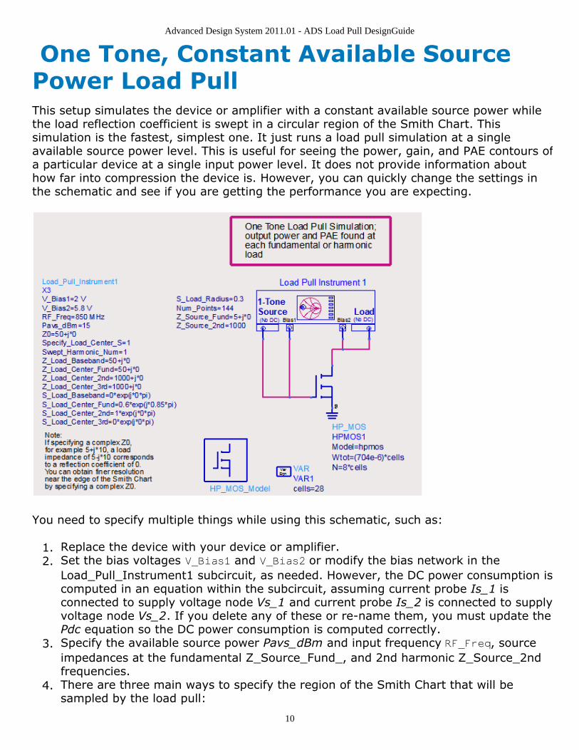
One Tone, Constant Available SourcePower Load PullThis setup simulates the device or amplifier with a constant available source power whilethe load reflection coefficient is swept in a circular region of the Smith Chart. Thissimulation is the fastest, simplest one. It just runs a load pull simulation at a singleavailable source power level. This is useful for seeing the power, gain, and PAE contours ofa particular device at a single input power level. It does not provide information abouthow far into compression the device is. However, you can quickly change the settings inthe schematic and see if you are getting the performance you are expecting.

You need to specify multiple things while using this schematic, such as:

Replace the device with your device or amplifier.1.Set the bias voltages V_Bias1 and V_Bias2 or modify the bias network in the2.Load_Pull_Instrument1 subcircuit, as needed. However, the DC power consumption iscomputed in an equation within the subcircuit, assuming current probe Is_1 isconnected to supply voltage node Vs_1 and current probe Is_2 is connected to supplyvoltage node Vs_2. If you delete any of these or re-name them, you must update thePdc equation so the DC power consumption is computed correctly.Specify the available source power Pavs_dBm and input frequency RF_Freq, source3.impedances at the fundamental Z_Source_Fund_, and 2nd harmonic Z_Source_2ndfrequencies.There are three main ways to specify the region of the Smith Chart that will be4.sampled by the load pull:


11

Set the reference impedance Z0 to 50, and set Specify_Load_Center_S=1. In1.this case, the center of the circle of simulated reflection coefficients (andharmonics) will be set by the S_Load_Center_* parameters, which are reflectioncoefficients.Set the reference impedance Z0 to 50, and set Specify_Load_Center_S=0. In2.this case, the center of the circle of simulated reflection coefficients (andharmonics) will be set by the Z_Load_Center_* parameters, which areimpedances.Set the reference impedance Z0 to the complex conjugate of the impedance at3.the center of the circle of reflection coefficients you want to simulate. In thiscase, you could set Specify_Load_Center_S=1 and use the S_Load_Center_*parameters. Remember that in this case, a reflection coefficient of 0corresponds to setting the load impedance to the complex conjugate of thereference impedance.

Specify the radius of the circle of the reflection coefficients S_Load_Radius and the5.number of points Num_Points.

If the device or amplifier is potentially unstable and the circle of reflection coefficients thatyou specify includes the unstable region, the simulation may run into convergenceproblems. This would be due to the device wanting to oscillate. A solution to this problemis to add stabilizing components at the input, output, or in parallel with the device. Youmay want to use a simulation setup for this purpose, DesignGuide > Amplifier > S-Parameter Simulations > Feedback Network Optimization to Attain Stability.Another solution is to specify the circle of reflection coefficients such that the unstableregion is avoided.You can select DesignGuide > Load Pull > Reflection Coefficient Utility to see a datadisplay with a graphical tool to help you see the circle that corresponds to particularvalues of the s11_rho and s11_center variables.

Run the simulation just as you would any other. When it finishes, open theHB1Tone_LoadPull data display.


12

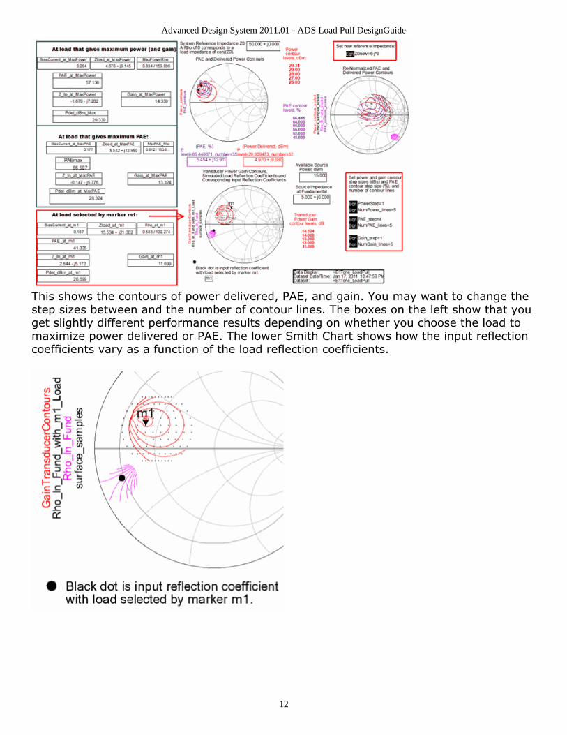
This shows the contours of power delivered, PAE, and gain. You may want to change thestep sizes between and the number of contour lines. The boxes on the left show that youget slightly different performance results depending on whether you choose the load tomaximize power delivered or PAE. The lower Smith Chart shows how the input reflectioncoefficients vary as a function of the load reflection coefficients.


13

One Tone, Constant Available SourcePower Load Pull with Swept ParameterThe One Tone, Constant Available Source Power Loadpull with Swept Parametersimulation allows you to see how the contours and performances vary with some arbitraryswept parameter (such as a bias voltage and the input frequency). However, the availablesource power is held constant.

This setup adds the sweep of an arbitrary parameter to the simplest constant availablesource power load pull simulation. You have to assign the parameter SweepVar to somecomponent or variable on the schematic. In this case it is assigned to the input signalfrequency RF_Freq.

The above figure specifies the limits of the swept variable, SweepVar, and assigning it toRF_Freq.

One Tone, Constant Available Source Power Source Pull

This setup simulates the device or amplifier with a constant available source power whilethe load reflection coefficient is swept in a circular region of the Smith Chart. Thissimulation is the fastest, simplest one. It just runs a load pull simulation at a singleavailable source power level. This is useful for seeing the power, gain, and PAE contours ofa particular device at a single input power level. It does not provide information abouthow far into compression the device is. However, you can quickly change the settings inthe schematic and see if you are getting the performance you are expecting.


14

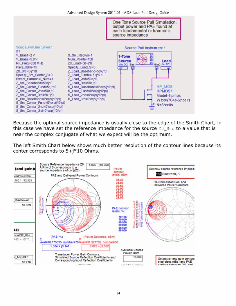
Because the optimal source impedance is usually close to the edge of the Smith Chart, inthis case we have set the reference impedance for the source Z0_Src to a value that isnear the complex conjugate of what we expect will be the optimum.

The left Smith Chart below shows much better resolution of the contour lines because itscenter corresponds to 5+j*10 Ohms.


15

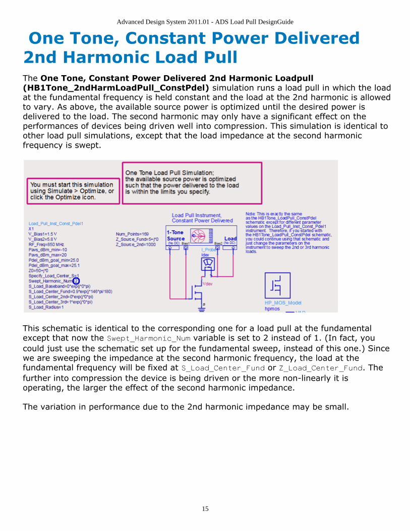
One Tone, Constant Power Delivered2nd Harmonic Load PullThe One Tone, Constant Power Delivered 2nd Harmonic Loadpull(HB1Tone_2ndHarmLoadPull_ConstPdel) simulation runs a load pull in which the loadat the fundamental frequency is held constant and the load at the 2nd harmonic is allowedto vary. As above, the available source power is optimized until the desired power isdelivered to the load. The second harmonic may only have a significant effect on theperformances of devices being driven well into compression. This simulation is identical toother load pull simulations, except that the load impedance at the second harmonicfrequency is swept.

This schematic is identical to the corresponding one for a load pull at the fundamentalexcept that now the Swept_Harmonic_Num variable is set to 2 instead of 1. (In fact, youcould just use the schematic set up for the fundamental sweep, instead of this one.) Sincewe are sweeping the impedance at the second harmonic frequency, the load at thefundamental frequency will be fixed at S_Load_Center_Fund or Z_Load_Center_Fund. Thefurther into compression the device is being driven or the more non-linearly it isoperating, the larger the effect of the second harmonic impedance.

The variation in performance due to the 2nd harmonic impedance may be small.


16


17

One Tone, Constant Power DeliveredLoad PullThe One Tone, Constant Power Delivered Loadpull(HB1Tone_LoadPull_ConstPdel) simulation optimizes the available source power leveluntil the desired power is delivered to each load reflection coefficient. You would use this ifyour device or amplifier needs to deliver a particular power level and you want to choosethe optimum load considering other performances (such as gain, gain compression, PAE,and bias current.)

This setup sweeps the load reflection coefficient in a circular region of the Smith Chart andoptimizes the source power level for each load reflection coefficient until the desired poweris delivered to the load. The data display shows contours of constant PAE, bias current,gain, and gain compression. The input reflection coefficient is also shown for a particularload that you specify. These data allow you to pick the optimal load that produces the bestPAE, gain, gain compression, or bias current, or make trade-offs amongst thesespecifications.

You have to make the same types of edits to this schematic as with the others describedabove . Also, you have to specify the minimum and maximum allowed values of theavailable source power, Pavs_dBm_min and Pavs_dBm_max, respectively.

During the optimization, the available source power is adjusted within these limits untilthe power that you want is delivered to the load. Depending on how high a power youwant delivered to the load and the gain of the device, you may have to adjust thePavs_dBm_max limit.

In this example, the power delivered (based on Pdel_dBm_goal_min and


18

Pdel_dBm_goal_max) is to be between 25 and 25.1 dBm. With this value and aPavs_dBm_max value of 20 dBm, it is specified that the lowest transducer power gainaccepted is 5 dB.You may also specify different load impedances or reflection coefficients at the harmonicfrequencies and (for the source) at the fundamental and harmonic frequencies.

To launch the simulation, click the Optimize icon . If the simulation is started by hittingthe F7 key or by selecting Simulate > Simulate, then an optimization is not executedand the simulation results are not displayed correctly in the data display.

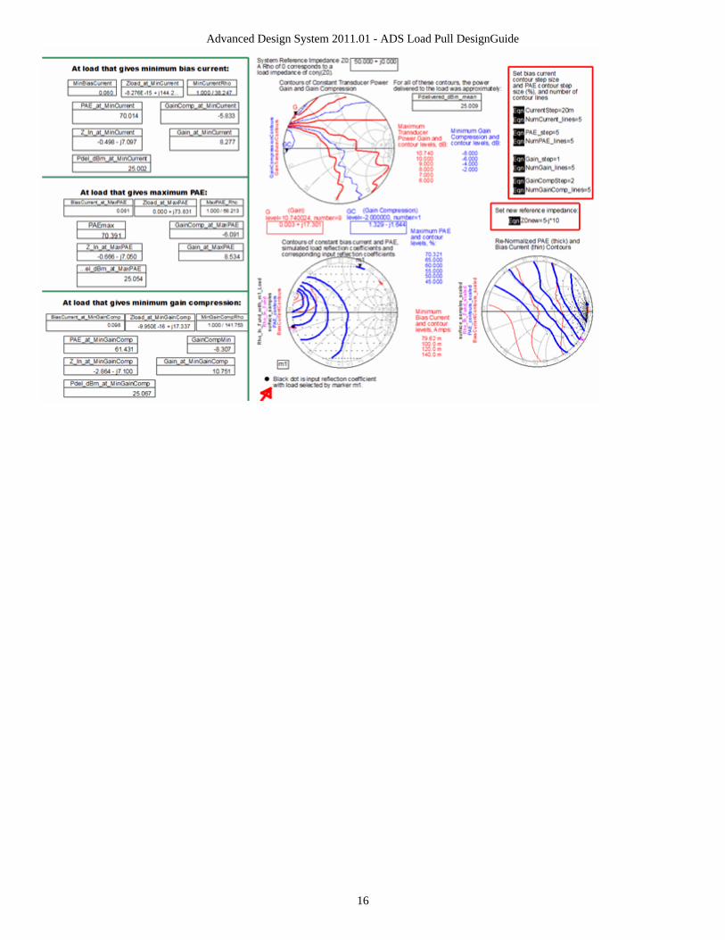
After running the optimization, the HB1Tone_LoadPull_ConstPdel data display showsthe results.

To see the contours effectively, you may need to change the CurrentStep, PAE_step,Gain_step, and GainCompStep variables. These set the step sizes between the contours.

The upper Smith Chart shows contours of constant gain and gain compression. The lowerleft Smith Chart shows contours of constant bias current and power-added efficiency(PAE), as well as the simulated load reflection coefficients and the corresponding inputreflection coefficients.

In the green boxes on the left side are data that correspond to a particular optimalcondition such as minimum bias current, maximum PAE, or minimum gain compression.However, you have to make sure that the desired power delivered was actually achieved.For some load impedances close to the edge of the Smith Chart this may be difficult.


19

You also have the option of selecting any of the simulated load reflection coefficients withmarker m1. The corresponding data appears in a separate box.

Data within the red box corresponds to the reflection coefficient selected by marker M1.


20

One Tone, Constant Power DeliveredLoad Pull with Swept ParameterThe One Tone, Constant Power Delivered Loadpull with Swept Parameter(HB1Tone_LoadPull_ConstPdel_Sweep) simulation adds the sweep of an arbitraryparameter. This sort of simulation is very useful if you want to see how the optimal loadimpedance, load pull contours, and the device performances vary versus some arbitraryparameter. For example, how does the optimal load vary with frequency and how do thepower added efficiency and other parameters change with the bias voltage. If you haveincluded some stabilization network around the device, how does the performance vary asyou change one of the parameters.

This simulation setup and data display are nearly identical to the version without theparameter sweep.

You have to assign the swept variable SweepVar to some parameter on the schematic aswell as set its sweep limits. In this case, the gate bias voltage V_Bias1 will be swept from1.5 to 2.25 Volts. After running the optimization, open theHB1Tone_LoadPull_ConstPdel_Sweep data display and make sure the default datasetname is set to the name of the dataset the simulation just created.


21

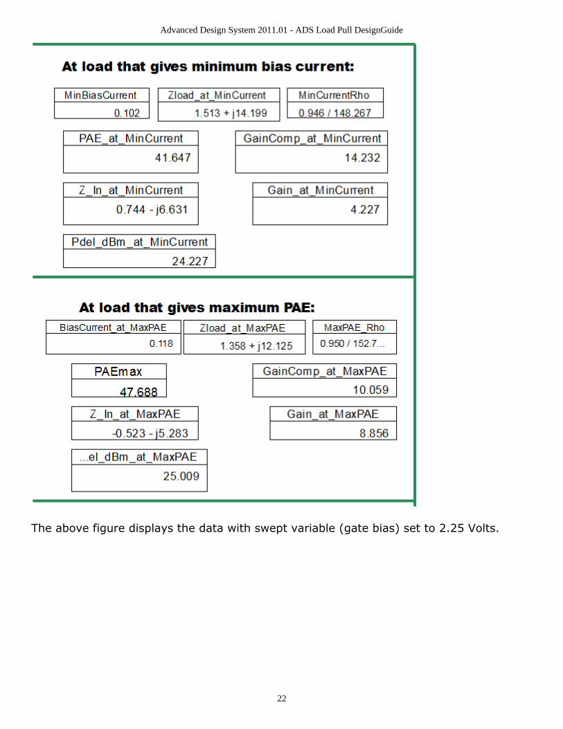
All the data is now indexed to the swept parameter value, which you select by moving theSweepIndx marker. There is a change in the power-added efficiency as you change thebias voltage.


22

The above figure displays the data with swept variable (gate bias) set to 2.25 Volts.


23

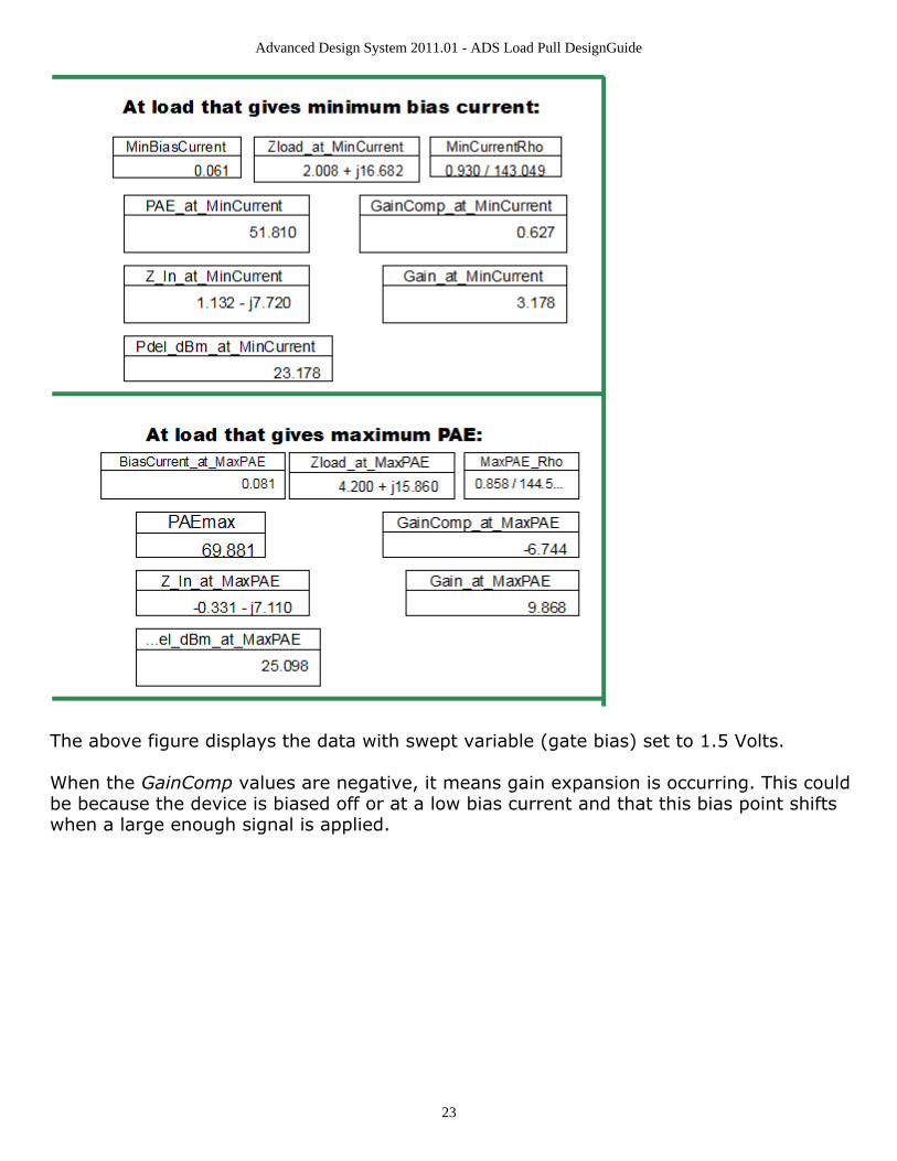
The above figure displays the data with swept variable (gate bias) set to 1.5 Volts.

When the GainComp values are negative, it means gain expansion is occurring. This couldbe because the device is biased off or at a low bias current and that this bias point shiftswhen a large enough signal is applied.


24

One Tone, Constant Power DeliveredSource PullThe One Tone, Constant Power Delivered Source Pull(HB1Tone_SourcePull_ConstPdel) simulation is most useful for determining theoptimal source impedance to present to a device. The source impedance should mostlyaffect the gain and gain compression. This setup sweeps the source reflection coefficientin a circular region of the Smith Chart and optimizes the source power level for eachsource reflection coefficient until the desired power is delivered to the load. The datadisplay shows contours of constant PAE, gain, and gain compression. This allows you topick the optimal source that produces the best PAE, gain, or gain compression, or maketrade-offs amongst these specifications.

The lower left SmallSignal and Sweep3 parameter sweeps are only used to obtain outputpowers when the device is being driven with a small signal. These output powers are usedas references in the gain compression computations.

Relative to the other constant power delivered simulation schematics above, the onlydifference is that you have to specify the constant load impedance at the fundamentalfrequency, instead of the source impedance. You may also specify different load andsource impedances at the harmonic frequencies. Typically, you would first run a load pullsimulation to determine the fundamental load impedance to use here.


25

To launch the simulation, click the Optimize icon. If the simulation is started by hittingthe F7 key or by selecting Simulate > Simulate, then an optimization is not executedand the simulation results are not displayed correctly in the data display.

After running the optimization, the HB1Tone_SourcePull_ConstPdel data display showsthe results.

To see the contours effectively, you may need to change the PAE_step, Gain_step, andGainCompStep variables. These set the step sizes between the contours. As statedabove, if you have modified the bias network, you will have to edit the Pdc equation onthe Equations page.

Also, the bias supply current calculations only include the current in the probe Is_high. Ifyou change the name of the current probe, you will need to edit the BiasCurrent equationon the Equations page.

The upper Smith Chart shows contours of constant gain and gain compression. The lowerleft Smith Chart shows contours of constant power-added efficiency (PAE) which may notvary much, as well as the simulated source reflection coefficients and the correspondinginput reflection coefficients, which may be just a single point since they should not dependon the source impedance. The lower right Smith Chart shows the same data on a SmithChart with a different reference impedance.

In the boxes on the left side are data that correspond to a particular optimal conditionsuch as maximum gain, maximum PAE, or minimum gain compression. However, youhave to make sure that the desired power delivered was actually achieved.


26

The source that corresponds to the maximum gain is very nearly satisfying the conditionsfor oscillation at the input (Z_In_at_MaxGain+Zsource_at_MaxGain =0, approximately),so you would want to avoid setting the source impedance to this value or you would wantto add some sort of stabilization network around the device.You also have the option of selecting any of the simulated source reflection coefficientswith marker m1. The corresponding data appear in a separate box.

The above figure shows the performance data corresponding to the source impedanceselected by marker 1. This enables you to see potential trade-offs. As you move awayfrom the maximum gain source impedance, the gain drops rapidly.


27

One Tone, Swept Available SourcePower Load PullThe One Tone, Swept Available Source Power Load Pull setup adds a sweep of theavailable source power for each value of the load reflection coefficient. It enables you tosee how the contours change as the device is driven from small signal to large signal intocompression. The schematic has an additional parameter sweep for the available sourcepower variable Pavs_dBm.

In addition to the various settings done in the HB1Tone_LoadPull schematic, you alsohave to specify the sweep limits for the Pavs (Power available from the source) variable.Here we have two ranges, one with a coarser step (assumed to be the linear region) andone with a finer step (in the compressed region.)

After running the simulation, open the HB1Tone_LoadPull_PSweep data display andmake sure the default dataset name is set to the name of the dataset generated by thesimulation.


28

The data display shows the transducer power gain, gain compression, power delivered,and PAE contours for a particular value of the available source power that you select usingSwpIndx marker. The gain and gain compression curves that correspond to severaloptimal load points (for minimum gain compression, maximum PAE, and maximum powerdelivered) are also shown.

Two Tone Simulation

Contents

Two Tone, Constant Available Source Power Load Pull (dgldpull)Two Tone, Swept Available Source Power Load Pull (dgldpull)Two Tone, Constant Power Delivered Load Pull (dgldpull)Two Tone, Constant Power Delivered Load Pull with Swept Parameter (dgldpull)


29

Two Tone, Constant Available SourcePower Load PullThis simulation setup and data display is identical to the "One Tone" version, except thatnow two tones are supplied instead of one. A two tone test signal stresses the devicemore because of its much higher peak-to-average ratio. The data display from thissimulation shows the same information as shown in the one-tone version and alsoincludes intermodulation distortion.

Here also you have to replace the sample device with yours and adjust the bias voltagesas needed. In addition to all the other variables that you must specify as before, you needto specify the following two variables:

Frequency spacing between the two tones F_Spacing.1.Maximum order of intermodulation distortion tones to be included in the simulation2.Max_IMD_Order.The simulation results include similar information as shown above, with the additionof intermodulation distortion.


30


31

Two Tone, Constant Power DeliveredLoad PullThis simulation setup and data display is identical to the "One Tone" version, except thatnow two tones are supplied instead of one. A two tone test signal stresses the devicemore because of its much higher peak-to-average ratio. The data display from thissimulation shows the same information as shown in the one-tone version and alsoincludes intermodulation distortion.

A different device is used here.


Frequency spacing between the two tones F_Spacing.1.Maximum order of intermodulation distortion tones to be included in the simulation2.Max_IMD_Order.

The simulation results include similar information as shown above, with the addition ofintermodulation distortion.


32

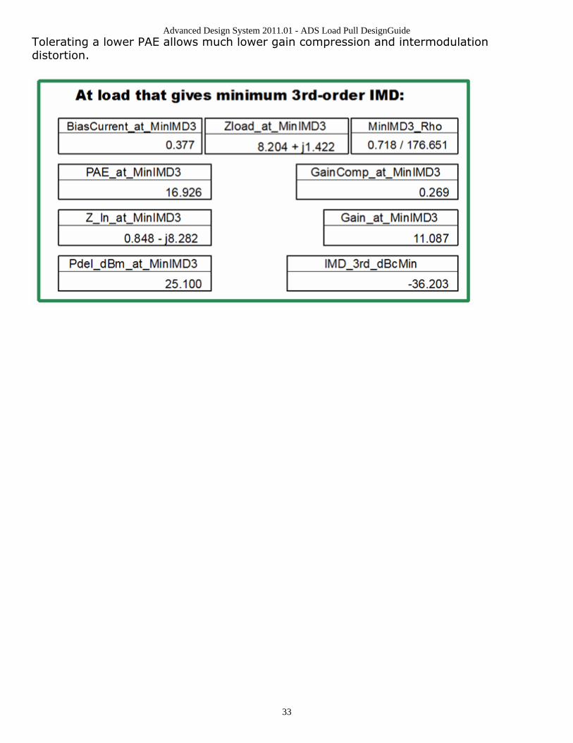
There is a clear trade-off between PAE and distortion. For this bias point, if you wantmaximum PAE, you suffer a lot of gain compression and intermodulation distortion.


33

Tolerating a lower PAE allows much lower gain compression and intermodulationdistortion.


34

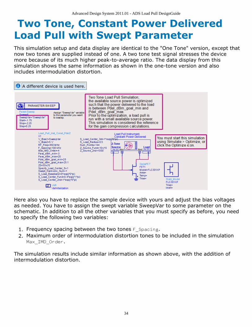
Two Tone, Constant Power DeliveredLoad Pull with Swept ParameterThis simulation setup and data display are identical to the "One Tone" version, except thatnow two tones are supplied instead of one. A two tone test signal stresses the devicemore because of its much higher peak-to-average ratio. The data display from thissimulation shows the same information as shown in the one-tone version and alsoincludes intermodulation distortion.

A different device is used here.

Here also you have to replace the sample device with yours and adjust the bias voltagesas needed. You have to assign the swept variable SweepVar to some parameter on theschematic. In addition to all the other variables that you must specify as before, you needto specify the following two variables:




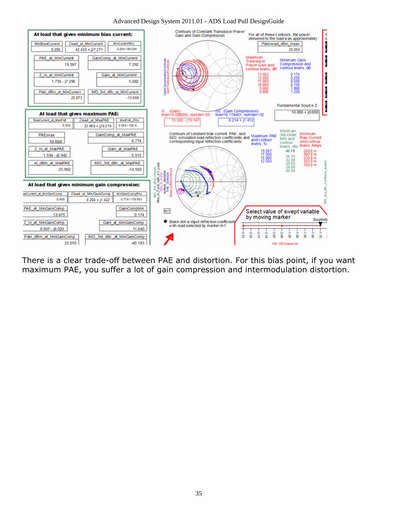
35

There is a clear trade-off between PAE and distortion. For this bias point, if you wantmaximum PAE, you suffer a lot of gain compression and intermodulation distortion.


36

Two Tone, Swept Available SourcePower Load PullThis simulation setup and data display is identical to the "One Tone" version, except thatnow two tones are supplied instead of one. A two tone test signal stresses the devicemore because of its much higher peak-to-average ratio. The data display from thissimulation shows the same information as shown in the one-tone version and alsoincludes intermodulation distortion.





37

WCDMA Signal SimulationWCDMA uses a source with WCDMA modulation instead of one or two sinusoids. Theadjacent channel power ratios are computed in addition to other performances such asgain, gain compression, and PAE. These simulations take longer to run, so you might wantto run at least one of the one- or two-tone simulations above first.

Select WCDMA Load Pull > Constant Power Delivered, Mag/Phase Load Pull tocopy WCDMA_LoadPullMagPh_ConstPdel schematic and corresponding data display intoyour workspace.

This setup sweeps the load reflection coefficient in a fan-shaped region of the Smith Chartand optimizes the source power level for each load reflection coefficient until the desiredpower is delivered to the load. The source is a WCDMA signal read in from a dataset, andits amplitude (and thus the available source power) is set by a variable, SFexp, and thegain applied to this signal is 10**(SFexp). The WCDMA signal was generated byconnecting a Timed Sink to the output of the signal source in the ADS exampleexamples/WCDMA3G/WCDMA3G_PA_Test_wrk/WCDMA3G_PA_UE_ACLR schematic.

The load pull is performed twice.

In first case, SFexp is set to 0.01. This is assumed to make the input signal small1.enough that the amplifier is operating linearly. The gain under this condition for eachload reflection coefficient is the reference used to compute the gain compression.In second case, SFexp is optimized until the desired power is delivered to the load.2.

The data display shows contours of constant PAE, ACLR, bias current, gain, and gaincompression. The input reflection coefficient is also shown for a particular load that youspecify. This allows you to pick the optimal load that produces the best PAE, ACLR, gaincompression, or bias current, or make trade-offs among these specifications.


38

When using this schematic, there are a number of different things you need to specify,and these are listed in a paragraph on the schematic. First, you would replace the devicewith your device or amplifier. You have to set the bias voltages or modify the biasnetwork, as needed. However, the data display calculates the DC power consumptionassuming current probe Is_low is connected to supply voltage node Vs_low and currentprobe Is_high is connected to supply voltage node Vs_high. If you delete any of these orre-name them, you will have to modify the equations likeIs_highDC=mean(Is_high.i[0]) and the Pdc equation on the schematic.

You have to specify the range of phases and magnitudes of the reflection coefficients. Thetotal simulation time will increase linearly with the product of the numbers of phases andmagnitudes simulated. The tradeoff is that you should get better contour lines with morepoints simulated.


39

If the device or amplifier is potentially unstable and the region of reflection coefficientsthat you specify includes the unstable region, the simulation may run into convergenceproblems. This would be due to the device wanting to oscillate. A solution to this problemis to add stabilizing components at the input, output, or in parallel with the device. Youmay want to use a simulation setup for this purpose, DesignGuide > Amplifier > S-Parameter Simulations > Feedback Network Optimization to Attain Stability.Another solution is to specify the range of reflection coefficients such that the unstableregion is avoided.

You also have to specify the reference impedance, Z0, and the source center frequency,RFfreq.

You have to specify the nominal and allowed range of the signal source gain scale factorexponent, SFexp. It is necessary to adjust this gain to set the available source power,because we are using a voltage source to generate the signal.

It is not obvious what the relationship is between this exponent and the available sourcepower. However, the WCDMA_SrcTest schematic in the same workspace allows you tosweep this scale factor and calculate the corresponding available source power. In thiscase, stepping SFexp from -1 to 1 increases the available source power from about -20dBm to +20 dBm. This does vary with the source impedance you specify.

When setting the range of SFexp values, you want the highest SFexp value to correspondto the maximum available source power you will accept. For example, if you want todeliver 27 dBm to the load and you want the device to provide at least 7 dB of transducerpower gain, you would set the maximum value of SFexp to correspond to an availablesource power of approximately 20 dBm. The optimization will run fastest if SFexp isallowed to vary over a relatively large range, but with the nominal value close to the valueneeded to give you the desired output power. You may get extremely high gaincompression values for some reflection coefficients near the edge of the Smith Chart.

Figure: Prior to starting on-screen editing


40

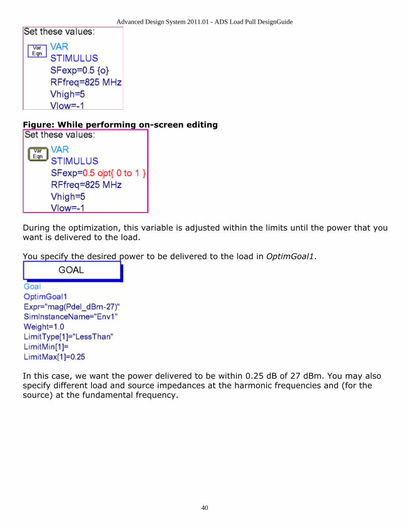
Figure: While performing on-screen editing

During the optimization, this variable is adjusted within the limits until the power that youwant is delivered to the load.

You specify the desired power to be delivered to the load in OptimGoal1.

In this case, we want the power delivered to be within 0.25 dB of 27 dBm. You may alsospecify different load and source impedances at the harmonic frequencies and (for thesource) at the fundamental frequency.


41

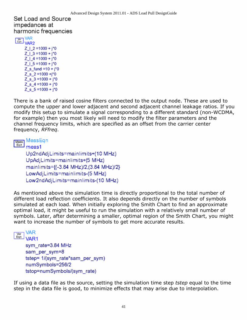
There is a bank of raised cosine filters connected to the output node. These are used tocompute the upper and lower adjacent and second adjacent channel leakage ratios. If youmodify this setup to simulate a signal corresponding to a different standard (non-WCDMA,for example) then you most likely will need to modify the filter parameters and thechannel frequency limits, which are specified as an offset from the carrier centerfrequency, RFfreq.

As mentioned above the simulation time is directly proportional to the total number ofdifferent load reflection coefficients. It also depends directly on the number of symbolssimulated at each load. When initially exploring the Smith Chart to find an approximateoptimal load, it might be useful to run the simulation with a relatively small number ofsymbols. Later, after determining a smaller, optimal region of the Smith Chart, you mightwant to increase the number of symbols to get more accurate results.

If using a data file as the source, setting the simulation time step tstep equal to the timestep in the data file is good, to minimize effects that may arise due to interpolation.


42

The Envelope analysis includes a SweepOffset. This simulates but does not keep the first12 symbols in the simulation during which the input signal amplitude is ramping on. If youwant to include this turn-on ramp data in the post-processing computations, just setSweepOffset=0.

Because the simulation includes an optimization, click Optimize icon to launch thesimulation. If instead you just launch the simulation by hitting the F7 key or selectingSimulate > Simulate, an optimization will not be run and the data display will notdisplay the simulation results.

After running the optimization, this WCDMA_LoadPullMagPh_ConstPdel data display showsthe results.


43

To see the contours effectively, you may need to change the CurrentStep, PAE_step,Gain_step, GainCompStep, and ACLR_step variables. These set the step sizes between thecontours. The bias supply current calculations only include the current in the probeIs_high. If you change the name of the current probe, you will need to edit theBiasCurrent equation on the Equations page.

The upper Smith Chart shows contours of constant gain and gain compression. The lowerleft Smith Chart shows contours of constant bias current, power-added efficiency (PAE),and lower adjacent channel ACLR, as well as the simulated load reflection coefficients andthe corresponding input reflection coefficients. The lower right Smith Chart shows thesame data on a Smith Chart with a different reference impedance.

In the red boxes on the left side are data that correspond to a particular optimal conditionsuch as minimum bias current, maximum PAE, minimum gain compression, or minimumACLR. However, you have to make sure that the desired power delivered was actuallyachieved. In some cases with load reflection coefficients very close to the edge of theSmith Chart, the desired power will not be achieved.

The results show there is a trade-off between power-added efficiency and distortion. Youcan get slightly better PAE if you are willing to tolerate higher ACLR levels.

Note that the power delivered specification is not satisfied. You could re-run thesimulation, allowing SFexp to vary over a larger range, or you could move marker m1 to aload near this one and see if the power delivered specification is satisfied. Moving markerm1 allows you to select any of the simulated load reflection coefficients. Thecorresponding data appears in a separate box, which allows you to see potential tradeoffsas you move around the Smith Chart.


44

The gain compression is still excessive, however.

The ACLR is somewhat sensitive to the load impedance.

The WCDMA Load Pull > Constant Power Delivered, Circular Region Load Pullmenu pick copies into your workspace a schematic and data display nearly identical to theWCDMA_LoadPullMagPh_ConstPdel ones above, except that it sweeps a circularregion of the Smith Chart instead of a fan-shaped region.

Time Taken by Simulation

For 25 different load reflection coefficients, numSymbols=128, and the optimization typeset to Gradient with MaxIters=5, this simulation required about 4 minutes. For 49different load reflection coefficients, about 6.75 minutes were required.

ADS Load Pull DesignGuide -...

Documents

Transcript of ADS Load Pull DesignGuide -...