Adoption of laser levelers and water- saving in agriculture · Adoption of laser levelers and...
55
Working paper Adoption of laser levelers and water- saving in agriculture Report on a follow up pilot study Nathan Larson Sheetal Sekhri Rajinder Sidhu February 2013
Transcript of Adoption of laser levelers and water- saving in agriculture · Adoption of laser levelers and...

Working paper
Adoption of laser levelers and water-saving in agriculture
Report on a follow up pilot study
Nathan Larson Sheetal Sekhri Rajinder Sidhu
February 2013

Adoption of Laser Levelers and Water-Saving in Agriculture:
Report on a Follow-up Pilot Study∗
Nathan Larson† Sheetal Sekhri‡ Rajinder Sidhu§
February, 2013
Abstract
Water saving agricultural technologies are a potentially important but under-
utilized lever to conserve groundwater in India. Technologies like laser levelers have
high private returns and lead to water savings, yet the adoption rates are not very
high. It is often thought that social influence is an important factor in adopting new
technologies. This report presents results from a pilot study in which farmers in the
Indian state of Punjab were surveyed about their beliefs about, and use of, laser
leveling, and about their social networks. This survey is a follow-up to an earlier
pilot study exploring similar issues; the earlier study provided valuable information
about laser levelers but not about social networks. In the current survey, a revised
elicitation procedure is used for social network information, with much greater suc-
cess.
∗Funding from International Growth Centre, India County Team is gratefully acknowledged. We
also thank Sonal Guarishanker and Martin Abel for superlative field assistance and research assistance
respectively.†University of Virginia; Email: [email protected]
‡University of Virginia; Email:[email protected]
§Punjab Agriculture University; Email: [email protected]
1

JEL classification: O10, O13, Q54
Keywords: Water Infrastructure, Groundwater Depletion India
1 Introduction
The rapidly declining stock of groundwater for irrigation poses a significant threat to
agriculture in India. As a result, there has been great interest in policies that could be used
to encourage farmers to adopt various water-saving technologies. This report discusses
the results of a pilot study on the adoption of one particular water-saving technology, laser
leveling. This pilot represents a follow up to an earlier IGC-funded survey in which over
800 farmers in the state of Punjab were asked about their perceived benefits and obstacles
to adopting laser leveling. One of the objectives of that earlier study was to map out the
farmers’social networks in order to shed light on the degree to which friends, family, and
other contacts influence a farmer’s attitudes and adoption decision. However, the network
mapping component of this first survey was unsuccessful, and the main objective of the
new study reported here was to correct this shortcoming by using a revised methodology
to elicit these networks. While this report will largely focus on this new network data,
farmers were also asked about their attitudes to and use of laser leveling, their irrigation
practices, and their agricultural practices more generally, and headline results on these
topics will be reported at the end.
The next two sections provide an abbreviated overview of the background context
of the study: we sketch the current situation with agricultural water policy in Punjab,
explain the role that laser leveling technology can play, and describe the key elements of
our earlier pilot study. (Readers who wish to delve deeper into these topics are encouraged
to refer to our earlier report.) After this preamble, we present the new results on social
networks from the current study, followed by a summary of other key findings. The report
concludes with discussion of options for a large-scale randomized controlled trial testing
how social networks can be enlisted to encourage adoption.
1

2 Background: Water Use and Laser Leveling
While India is the largest user of groundwater in the world (with heavy demand from both
agriculture and households), current patterns of groundwater use are not sustainable in the
long run. Water tables are falling rapidly, in large part due to the fact that individuals
do not bear the cost of the water they use: free water extraction is a property right
attached to land ownership, and the electricity needed to pump water to the surface is
highly subsidized. If current trends continue, some estimates suggest that national food
production could fall by around 25 percent by 2025 (Seckler et al, 1998).
In principle, the best policy to curtail over-extraction would be to price water at its
social marginal cost, or barring this, to end the electricity subsidy that makes pumping
water effectively free. However neither of these is practical in the short run; the first would
require metering and monitoring millions of private wells nationwide, while the latter is
politically problematic. Given these limitations, there is a strong argument that policy
intervention to encourage the use of water-saving technologies is a logical second-best
measure.
Laser leveling is one such technology: in brief, it is a method of smoothing agricultural
fields to high precision by using laser guidance. Laser leveling is an “add-on”technology,
in the sense that it supplements rather than replaces the traditional method of leveling
a field. In traditional leveling, a grading implement with a blade is towed behind a
tractor over the surface of a field; the height of the blade is adjusted manually by the
operator so as to achieve a surface that appears smooth and level to the human eye.
The innovation in laser leveling is to use a laser guidance system to raise and lower the
blade of the grading implement automatically. The result is a significantly flatter field
than an unaided human operator could achieve. Evidence suggests that the benefits of
leveling can be substantial. In controlled experiments on agricultural plots, researchers at
Punjab Agriculture University found that laser leveling increases crop yields by around
11 percent and results in water saving of around 25 percent, holding constant other inputs
like fertilizers and seed quality. These experiments have also demonstrated that leveling
reduces weeds by up to 40 percent and labor time spent weeding by up to 75 percent (Bhatt
2

and Sharma). However, because these results were achieved by academic researchers
implementing best practices, it remains to be seen whether real farmers operating in
uncontrolled conditions will achieve similar benefits. Assessing this question was one
purpose of our study.
2.1 Laser Leveling in Punjab
In Punjab, where both of our studies were conducted, village agricultural cooperative
societies play a central role in providing access to laser leveling for farmers. These co-
operatives, largely established in the last decade, offer a variety of services to farmers,
including equipment rental, seed and fertilizer sales, and short term loans. In the last
six years, the state of Punjab has encouraged them, by means of a 30% subsidy on the
purchase price, to acquire laser levelers that are then made available for rental by farmers.
At present, there are over 2000 laser leveler units in service in Punjab, most owned by
cooperatives.1 While the up-front rental cost to farmers is significant (500 rupees/hr, or
roughly 750 rupees/acre), past evidence suggests that the private returns (in higher yield
and lower labor costs) are high enough to recoup that investment within one to two years
(Jat et al., 2009), and that the benefits of leveling persist for five years or more. Thus,
leveling could be a compelling investment for farmers even if they do not internalize the
positive externality of reduced water use. Despite its benefits and wide availability, adop-
tion of this technology remains relatively low —in Punjab prior estimates indicate that
only one-seventh of all cultivable land has been laser leveled.
2.2 Rental Arrangement
Cooperatives charge 500 rupees per hour for the rental service, or approximately $9 at
current exchange rates. Renting a leveler is an all-inclusive service: the cooperative
provides all the necessary equipment (the leveler, the grading implement, and the tractor)
and the driver; no effort from the farmer is required besides paying the fee. The farmer
1There are a relatively small number of private owners, most of whom have large landholdings. For a
smaller farmer, purchasing a laser leveler would not be cost effective.
3

pays only for time spent in-field, not transportation time to and from the field; a typical
estimate for the time required to level a field is 1.5 hours per acre. Most cooperatives
will own a single laser leveler, so in principle scheduling limitations could prevent some
farmers who would like to schedule a rental from doing so; we will discuss evidence on
this point below. The purchase cost of a leveler is high enough to make owning one
impractical for all but the very largest landowners. While in principle there is nothing to
prevent a private market in laser leveler rentals, in practice most rentals appear to take
place through the village cooperative.
3 The Earlier Study
The earlier study was based on a survey designed to illuminate farmers’adoption deci-
sions, including the channels through which they learn about laser leveling, the beliefs
they hold about the benefits and costs to adoption, and the obstacles to adoption that
they face. Going into the survey, we anticipated that two types of obstacle, financial
constraints and lack of knowledge about the technology, might be particularly important.
Financial constraints would come into play if, for example, small farmers found themselves
particularly cash constrained at times just before sowing a new crop, as this happens to
be the appropriate time to level one’s fields. In other settings, cash constraints around
the time of sowing are known to be a problem (Duflo et al., 2010). Alternatively, if farm-
ers are unaware of, or misinformed about the benefits of laser leveling, adoption might
be low. Other studies of technology adoption provide some evidence of breakdowns in
information flow in this region: farmers complain that they are underserved by offi cial
information channels, such as visits from agricultural extension offi cers and technology
demonstrations, and they list neighbors and family as an important source of information
about agricultural practices (Jafry, 2007). In particular, small and female farmers were
more reliant on socially transmitted information than large farmers were. One focus of our
study was to collect information about both offi cial channels and informal social network
channels by which farmers learn about new technologies.
4

4 Study Design
We carried out the first survey in the state of Punjab in India, in the districts of Amritsar
and Jalandhar. In addition to the reasons described earlier, Punjab is of interest because
it produces a large fraction of the rice grown in India. (The crop yield and water saving
benefits of laser leveling are considered to be greater for rice cultivation than for other
crops because the typical method of irrigation is to flood the field to a depth of 2.5 to 3
inches.) The study consisted of a survey administered to households in eight villages; the
objective was to reach every farming household in each of those villages. The procedure
for choosing these villages and the content of the survey are described briefly below.
4.1 Village and Respondent Selection
One objective of the earlier study was to understand why some farmers have adopted laser
leveling while others have not. For this reason, one criterion in selecting villages for the
survey was to include villages with a range of different adoption rates. A second goal was
to study both early-stage (right after the technology has been introduced) and later-stage
adoption. Thus, we looked for villages in which the first laser leveler was acquired at
different dates.
To make the selection, we obtained a list of all the cooperatives in two districts,
Amritsar and Jallandhar, that currently offer laser leveler rental. This list included the
date at which each cooperative acquired the leveler, and an estimate of the fraction of
land leveled in the village. Using this list, we chose eight villages spanning a range of
acquisition dates (from early 2007 through late 2010) and estimated adoption rates. In
each village, the goal was to survey all land-owning farmers. In total, we surveyed 856
individual land-owning farmers across the eight villages.
4.2 Results
The results of this first pilot indicated that both financial constraints and poor information
act as barriers to the use of laser levelers by farmers in Punjab. Both of these barriers tend
to create a divide between farmers with larger landholdings and smaller (and presumably
5

poorer) farmers. It is not surprising that financial constraints hit small farmers harder, but
it turns out that larger farmers, particularly those with connections to local government,
are also better informed about the benefits of laser leveling. This suggests that a policy
intended to promote laser leveler use across farmers of all sizes may need to tailor its
approach differently to different socioeconomic groups. Our original plan was to map
out social networks in the surveyed villages in order to study how patterns of social
relationships relate to patterns of adoption. However, the network mapping was largely
unsuccessful; correcting the problems with this mapping was the main purpose of the new
study we report on here.
5 Design of the New Study
Our current study was designed to correct problems that arose with mapping social net-
works during the first pilot. Using a revised network elicitation method, an updated
survey was administered to farmers in a different set of villages than those visited pre-
viously. The process for selecting villages was similar to the first pilot except that this
time villages in three districts, Amritsar, Jallandhar, and Ludhiana, were considered. As
before, we chose villages spanning a range of laser leveler acquisition dates and estimated
adoption rates, and also as before, the full survey was administered to each land-owning
household in a village. In total, the new study comprises five villages with a total of 479
land-owning households.
Except for the changes to the social network module, the content of the survey was
largely the same as in the first study, but some questions were streamlined or eliminated
to avoid redundancy. One exception is on irrigation practices where a suite of questions
were added. One concern behind these questions is that while laser leveling may make
it possible for a farmer to use less water, these savings will not occur unless he adjusts
his irrigation practices. To understand whether this adjustment is likely to happen, it is
important to understand the incentives that govern current practices.
6
5.1 Network Elicitation Methodology
In the earlier pilot, survey enumerators were instructed to ask each respondent to list
people within the village with whom he (the farmers are almost universally male) com-
municated about agricultural matters. There were several diffi culties with this approach,
which we have sought to respond to in the latest pilot: (1) compliance was poor, in the
sense that many respondents did not volunteer any names; (2) while all farming house-
holds in a village were surveyed, matching the identities of a respondent’s listed contacts
to their household surveys proved to be problematic; (3) anecdotal reports suggest that
some farmers were reluctant to go “on the record”about seeking farming advice out of
a sense of pride; and (4) respondents tended to name people in formal positions, such as
the cooperative secretary or shopkeeper, even when the natural answer to the question
would be friends or family. On the last point, farmers were asked about their networks
after a long series of questions on agricultural practices, so it is possible that they were
inadvertently primed to think of more offi cial sources of agricultural information.
In the updated pilot, while the tenor of the questions about social networks was gen-
erally similar, the methodology for eliciting responses was rather different. Most impor-
tantly, social network information was collected in two stages. In the first stage, prior to
the main survey, our enumerators canvassed each village to form a roster of all households,
including the names of the head of household and of any other co-resident farmer, with
each household assigned a unique numerical identifier. Then, some time later, enumera-
tors returned to carry out the main survey including the questions about social contacts.
The roster was brought along, and when network questions were asked, the respondent
was encouraged to pick out his contacts from the roster. These contacts were recorded
by ID code, ensuring that they could be matched to their own survey responses. This
methodology appears to have drastically improved both matching and compliance: farm-
ers volunteer more names and those names appear less likely to be mismatched to the
question. Furthermore, we suspected that both issues (3) and (4) above stemmed in part
from the long series of agricultural questions at the beginning of the survey which may
have induced farmers to filter their social contact responses based on a sense of what the
7

“correct”answers should be. In the updated survey, social contact questions were asked
at the beginning of the survey so that respondents would not form preconceptions about
how to answer. In addition, language about “relying on others’opinions”was softened to
avoid any insinuation about whether the respondent was self-reliant or not.
6 Results
6.1 Summary Statistics About Farmers’Social Network Con-
tacts
This section provides an in-depth look at the social networks in the five villages in which
we collected this data. These villages comprise 1227 households in total, approximately
381 of which own land; our social network questions were addressed to these landowning
households.
Table 1 provides summary statistics about the average number of contacts reported by
each farmer for five types of relationship: relatives, friends, people he spoke to at least five
times in the last month (“5X,”or “spoken,”for brevity), farmers with neighboring plots,
people with a reputation (according to the respondent) as knowledgeable and successful
farmers. The first four categories involve what we will refer to as two-way relationships,
in the sense that one would expect the contact to cite the same relationship with the
respondent. For example, if A claims B as a relative, then B’s list of relatives should
include A. We refer to the last category as a one-way relationship because the fact that A
regards B as prominent and respected does not necessarily imply the converse is also true.
These five categories are intentionally broad and neutral; except in the last case there
is no suggestion that respondents should frame their answers in terms of preconceptions
about how agricultural information should spread.
The next two questions in Table 1 focus more sharply on how much farmers know
about the laser leveling decisions of other in their village. These questions were inten-
tionally asked at the end of the social network module to avoid coloring the responses to
earlier questions. Specifically, a farmer was asked who, to his knowledge, had adopted
8

laser leveling before he did (or at all, if the respondent had never adopted), and who
had adopted laser leveling after he did. These questions will not prove whether adoption
spreads by social influence, but they may be helpful in determining whether this is plau-
sible or implausible. For example, it is harder to argue that farmer B was influenced by
farmer A’s adoption decision if he does not report knowing about it.
The median number of contacts reported for each category is usually one or two. The
median number of people talked to is zero, but this may be because we asked the farmers
to identify farmers talked to 5 times in last month which may have been mis-construed.
Interestingly, there is relatively little overlap in the contacts a farmer reports for the
different types of two-way relationship: the median total number of distinct relatives,
friends, 5X contacts, and plot neighbors is seven. This lack of overlap may be genuine,
but we cannot be sure —some respondents may have assumed that they were meant to
list a contact in only one category, even though they were not told to do this.
The analysis in the next section will take up the question of whether a farmer’s decision
to adopt laser leveling is influenced by any prior experience that his social contacts have
with the technology. Before plunging into this question, it is helpful to have a sense of the
general pattern of adoption by a farmer’s social contacts. For our purposes here, let us
normalize Year 1 for a village to be the earliest year that any farmer in the village reports
adopting laser leveling. Figure 1 reports the probability in Year t (where t = 1, 2, ..., 6)
that a farmer has at least one social network contact who has adopted laser leveling by
Year t or earlier. (This trend is labeled as “Any.”) On the same figure, we report the
same probability broken down by relationship type: that is, the chance that a farmer has
at least one relative who has adopted by Year t, or at least one friend, and so forth.
In the first year, only 25% of farmers have any social contact who has adopted, but this
percentage rises steadily over time and in the most recent crop season, almost every farmer
has such a contact. We see a similar gradual rise in the probabilities of knowing an adopter
in each of the relationship categories, but there is a clear difference between social contacts
who are prominent, knowledgeable farmers and those in the other categories. At every
point in time, contacts who are viewed as prominent and knowledgeable are substantially
more likely to have adopted than contacts in the other categories. Furthermore, this
9

gap widens substantially between Year 2 and Year 3 with the other categories catching up
gradually, if at all, in later years. Altogether, this would appear to suggest that prominent,
knowledgeable farmers may be a particularly critical source of information for others in
the early years of the adoption process.
6.2 Peer Effects in the Adoption of Laser Leveling
Our principal motivation for collecting data on farmers’social networks is to study the role
that these networks play in spreading word of mouth about laser leveling and convincing
farmers to try it. In order to address this question, we will focus on lagged peer effects
models in which a farmer’s likelihood of adopting laser leveling for the first time may
depend on the past adoption decisions of some subgroup of farmers in his village —which
we call his reference group — as well as other factors. The premise of such models is
that adopters pass on information about laser leveling to those who have not yet adopted
and that this additional information can be instrumental in convincing non-adopters to
try the technology. For our purposes here, we will be agnostic about the form that this
information takes. For example, it may be that adopters talk about their outcomes, such
as successful crop yields, water savings, and so forth. Alternatively, it could be that the
very fact that they adopted, which reveals their confidence that laser leveling will be
worthwhile, is the final straw that convinces others to follow suit.
To illustrate the approach, a very common specification for studying peer effects in
technology adoption is the following
Pr (i adopts at time t | has not adopted so far) = f (βAvt−1 + γXi)
where Avt−1 represents the cumulative fraction of farmers in individual i’s village v who
had adopted at time t− 1 or earlier, and Xi is a vector of characteristics of individual i.
In order to interpret this as a model of word of mouth, we make the assumption that a
farmer interacts more or less uniformly with all of the other farmers in his village. Then
we can think of Avt−1 as the chance that farmer i interacts with another farmer who has
already adopted laser leveling and passes on information that helps to persuade i to adopt.
Notice that in this model, a farmer’s reference group includes everyone in his village; with
10

this in mind, let us call it the Village Peer Effect model. A second point to note is that we
must be cautious in interpreting results from this model —a positive coeffi cient β could be
evidence for the story above, but there are other interpretations that cannot be excluded.
For example, it could be that farmers face pressure to conform with typical practices in
the village, and so they tend to adopt when Avt−1 is large simply to fit in, not because
they have learned from past adopters.
Under the model above, social networks do not play any special role in the spread of
adoption; in effect, everyone in a village who has already adopted influences farmer i’s
adoption decision equally. A natural alternative is to suppose that a farmer is influenced
only by his social network contacts. Write this schematically as
Pr (i adopts at time t | has not adopted so far) = f (β PeerAdoptionit−1 + γXi)
where PeerAdoptionit−1 is some summary measure reflecting adoption at time t − 1 or
earlier by farmer i’s network contacts. To distinguish this case, we call it the Network
Peer Effect model. Recall that in our data, farmers classify their social contacts into five
types of relationship: relatives, friends, those spoken to at least five times in the last
month, plot neighbors, and farmers regarded as knowledgeable. For our purposes here,
we consolidate those categories into a single class: individual j is regarded as a peer of i,
written j ∈ {Peersi}, if i lists j as a contact under any of these five relationships.
While there are any number of ways that a farmer could be influenced by his peers’
past adoption, we will focus on three plausible specifications of the PeerAdoptionit−1
summary variable. The first is PeerAdoptionShareit−1, which is defined as the fraction
of farmer i’s peers who adopted laser leveling at time t − 1 or earlier. The second,
PeerAdoptionNumberit−1, is simply the total number of peers who adopted at t − 1 or
earlier. Finally, PeerAdoptionAnyit−1 is an indicator variable equal to 1 if farmer i has at
least one peer who adopted by time t− 1. These variables represent different conceptions
of how much evidence a farmer might require to be persuaded that laser leveling is a
good idea. The first two, the share and the total number, would be appropriate if farmers
require an accumulation of evidence, or information, from different people in order to be
convinced to adopt. If all farmers had the same number of contacts, these two variables
11

would be essentially equivalent; to see the difference between them, consider a scenario
in which farmer A has 5 peers while farmer B has 10, and the farmers are identical on
other dimensions. If each has one peer who has adopted laser leveling, the total number
specification stipulates that A and B will be equally likely to adopt, while the share
specification stipulates that A will be more likely to adopt since one peer is a larger
fraction of his contact list.
In contrast with the other two, the third variable, PeerAdoptionAnyit−1, would be
appropriate if knowing at least one contact who has adopted is the critical element in
tipping a farmer’s decision, and if additional examples of adoption do not add much
additional information. This might make sense if many farmers are already close to
adopting and just need an additional nudge; for example, it may be that farmers have
heard, and accepted in theory, the claims made about benefits from laser leveling, but
they would like to see at least one piece of hard evidence before adopting.
To estimate these peer effects models, we use the Cox proportional hazards specifica-
tion for the link function f :
Pr (i adopts at time t | has not adopted so far) = h (t) eβAvt−1+γXi+µv
for the Village Peer Effect model, or
Pr (i adopts at time t | has not adopted so far) = h (t) eβPeerAdoptionit−1+γXi+µv
for Network Peer Effects. Under this specification, the hazard rate for adoption is the
product of a common baseline hazard rate h (t), which is allowed to have a flexible form and
is not estimated, and a shifter term that expresses farmer i’s likelihood of adoption relative
to the baseline. We also allow for village fixed effects µv to capture unobserved factors
— for example, a particularly industrious cooperative secretary —that affect all farmers
within a village. The survey records date of first adoption by month and year; for our
initial specifications, we aggregate so that time t is measured in years. However, because
the rice crop season extends over the summer months, there is a qualitative difference
between an adoption in April 2010, which occurs in time to have an effect on the 2010
crop, and an adoption in October 2010 whose effects will not be seen until the 2011 crop.
12

With this in mind, we break each year between July and August: adoptions prior to
the break point are attributed to the current year, while later adoptions are attributed
to the next year. The vector of farmer characteristics Xi includes total landholdings (in
acres), self-reported land quality, indicators for belonging to a scheduled caste and for
membership in the cooperative society, age, years of education, and an indicator variable
for “government connections.” (The latter is equal to one if the farmer reports ties to
offi cials such as the cooperative secretary, local council members, or district and state
level offi cials.)
Regression results are presented first without village fixed effects (Table 4) and then
including them (Table 5).2 In the absence of fixed effects, lagged adoption appears to
have a positive and significant effect whether one considers the Village Peer Effect model
or the Network Peer Effect models based on the share of prior adopters among one’s peers
or knowing any prior adopter. (The effect of the number of prior adopters among one’s
peers is insignificant.) However, we must be cautious in interpreting these results, as the
effect that we attribute to peer influence could actually be due to unobserved differences
across villages. To illustrate, suppose that Village A has a cooperative secretary who,
unbeknownst to us, is unusually enthusiastic about promoting new technology. This fact
will tend to make new adoption higher in every time period than we would otherwise
expect, based on the observed characteristics of farmers in Village A. Then because high
adoption will tend to follow high adoption in Village A, while lower adoption will tend
to follow lower adoption elsewhere, the statistical estimation may tend to reconcile this
pattern by imputing an inflated, or even spurious, positive effect of lagged adoption on
current adoption. By including fixed effects in Table 5, we hope to control for such
spurious effects. However, before moving on, let us note some of the other factors that
appear to influence adoption. A farmer is significantly more likely to try laser leveling if
he owns more land, has government connections, or does not belong to a scheduled caste.
Moreover, being younger or being a member of the cooperative society has a significant
positive effect on adoption in at least some of the specifications.
We turn next to the specification with village fixed effects in Table 5. One will imme-
2All standard errors are clustered at the village level.
13

diately notice an important change in the Village Peer Effect model: the sign on lagged
adoption flips from positive to negative and insignificant. While this is a curious result, it
would probably be unwise to make too much of it. Because lagged village adoption Avt−1
and the village fixed effect µv are both constant across all farmers within a village at time
t, the only way to identify an effect of Avt−1 separately from µv comes from variation
within a village over time. However, the time series is not long enough to separate the
effects of Avt−1 and µv with much precision.
The coeffi cients in the Network Peer Effect models are better identified because farmers
within a village have different sets of social contacts, creating within-village variation
in the PeerAdoptionit−1 variables. While the effect of the number of prior adopters
among one’s peers is small and no longer significant, the effects of the other two variables,
PeerAdoptionShareit−1 and PeerAdoptionAnyit−1, remain positive and significant. The
most natural way to interpret the coeffi cients on these variables is through the hazard
ratio eβ. For example, for the “Peer Any”specification, if there are two otherwise identical
farmers, one of whom has has at least one peer who has adopted laser leveling and another
who has not, the first farmer will be eβ ≈ 1.51 times as likely to adopt as the second one.
Most of the other factors that were significant predictors of adoption in Table 4 remain
so, and with similar magnitudes, in Table 5; the exceptions are age, which is no longer
significant, and cooperative membership, which emerges as a positive and consistently
significant factor. While we do not have direct measurements of wealth and social class,
the pattern of results strongly suggest that richer, upper class, and better connected
farmers are relatively more likely to adopt laser leveling. For example, the coeffi cient on
landholdings, which is consistently in the neighborhood of 0.03, indicates that raising a
farmer from the 25th percentile of landholdings to the 75th percentile (from 2 acres to 8.5
acres), will raise his likelihood of adopting by a factor of e0.03(8.5−2) ≈ 1.22.
The results in Tables 4 and 5 suggest that social network structure materially affects
the way that knowledge and use of a new technology spread. That is, average behavior in
the whole village is not enough to explain who adopts and who does not; one must also look
at the individualized information conveyed by each farmer’s friends and family. To provide
more convincing evidence that this is the case, we estimate hybrid models that include
14

both lagged adoption in the entire village and lagged peer adoption at the same time. We
focus on the two peer variables that were consistently significant earlier, Share and Any,
and omit village fixed effects to give Ait−1 its best chance to knock the peer variables out
of significance; these estimates are presented in Table 6. In both cases (columns 1 and 2),
the effect of one’s social network peers remains significant and changes little in magnitude
when village-level adoption is included as an explanatory factor, indicating that peers are
influential over and beyond the overall trend of adoption in one’s village. In column 3
of the table, the two peer effect variables are allowed to compete with each other. In
this case, PeerAdoptionShareit−1 appears to be a stronger predictor of behavior than
PeerAdoptionAnyit−1: the effect of the latter shrinks and becomes insignificant, while
the share of one’s peers who have adopted remains positive and significant.
Month by month adoption
One limitation of studying adoption on a year by year basis is that we treat some
adoptions as contemporaneous when they really occur in sequence. For example, if two
farmers adopt in March and April of the same year, it is reasonable to think that the first
farmer’s decision might have influenced the second farmer; however, our analysis thus
far does not allow for this possibility since the farmers are treated as adopting at the
same time. Next, in order to examine how this issue affects our results, we re-estimate
some of our earlier specifications treating a month as the unit of time rather than a year;
the results are in Table 7. Column 1 includes PeerAdoptionShareit−1, column 2 uses
PeerAdoptionAnyit−1, and column 3 includes both. In this month-by-month specification,
the relative importance of the two peer effect variables appears to flip: having at least
one prior adopter among one’s peers is a positive and significant predictor of one’s own
adoption, both on its own and in concert with PeerAdoptionShareit−1. In contrast, the
share of prior adopters has the wrong sign and is weakly significant to insignificant. We do
not have a compelling explanation for this difference in the results at annual and monthly
frequencies; it is probably safest to say that while a farmer’s social network contacts have
a robust effect on his decision to try laser leveling, the exact functional form of that effect
is not conclusively revealed in the data.
Because of the difference in the unit of time, the coeffi cients in Table 7 cannot be
15

compared directly with their counterparts in the earlier tables. For example, if we use
the coeffi cient on PeerAdoptionAnyit−1 in column 2 to compute a hazard ratio, we have
eβ ≈ 1.39. As before, this has the interpretation that having at least one social contact
who has used laser leveling boosts a farmer’s likelihood of adopting by a factor of 1.39.
However, one must remember that this is now the additional likelihood of adopting within
the current month; the likelihood of adopting anytime within the next year (that is, the
next 12 months beginning with the current one), will presumably rise by an even greater
factor. In this sense, the strength of peer effects appears to be greater when measured
at a monthly frequency than at an annual frequency. It would be imprudent to draw
firm conclusions about why this is true, but we can cautiously speculate. One possibility,
as suggested above, is that by overlooking those peers of a farmer who adopted earlier
than him, but in the same year, the annual data tends to underestimate peer effects by
overlooking one source of influence. If so, the fact that the “annualized”effect of a peer
adopter appears to grow so substantially when switching to monthly data may suggest
that within-year peer effects are particularly strong. To put this point more plainly, it
may be that farmers tend to adopt right after their friends do —perhaps because the idea
is fresh in their minds —but that if they do not strike while the iron is hot (so to speak),
the potency of the friend’s example begins to fade. To examine this hypothesis more
carefully would be stretching our existing data rather finely, but it is not inconceivable;
for the time being we will leave it as a conjecture.
Which types of relationships matter for adoption?
Thus far, our analysis has proceeded on the implicit assumption that all of a farmer’s
social network contacts influence him in more or less the same way. However, it may
be that certain types of contacts —prominent, knowledgeable farmers, for example —are
particularly influential sources of information about laser leveling, while other types of
contact matter relatively less. Because our data include the nature of the relationship
between farmer and contact, we can examine this hypothesis. Our results here expand
on the “any peer”specification in the monthly data just discussed. For each of the five
relationship categories, relative, friend, spoken to at least five times in the last month,
plot neighbor, or prominent, or knowledgeable farmer, we create a dummy variable equal
16

to one if a farmer has a contact in that category who has already adopted. For example,
FriendAnyit−1 will be equal to one if farmer i has at least one friend who adopted at time
t−1 or earlier. Table 8 presents peer effects specifications including PeerAdoptionAnyit−1with each of these relationship dummies individually (columns 1-5) and all together (col-
umn 6). If prior adoption by a certain type of social contact carries relatively more weight,
this should show up in a positive and significant coeffi cient on the appropriate dummy.
As the table demonstrates, the significant positive effect of having at least one prior
adopter among one’s peers is robust, and its size hardly changes across the specifications.
However, we find no evidence that the nature of one’s relationship with a prior adopter
matters: all of the relationship coeffi cients in columns 1-5 are small and (with one excep-
tion) insignificant. The story is essentially the same when we compare all five relationship
types at once. In both cases, the single exception is the significant negative coeffi cient on
SpokenAnyit−1, suggesting that word of mouth from farmers spoken to frequently in the
last month may be somewhat less influential than other sources.
Does the influence of social networks vary with farmer size?
The fact that larger farmers (those with more land) adopt laser leveling at higher
rates is a very consistent thread running through the results reported so far. As discussed
elsewhere, a farmer’s landholding size is likely to be correlated with a number of other
characteristics of interest that we do not observe (or observe imperfectly), such as his
wealth, entrepreneurial spirit and openness to new technology, and access to offi cial infor-
mation channels and credit markets. Since large and small farmers are likely to differ on
all of these dimensions, it is natural to ask whether they also differ in the extent to which
they rely on peer networks for guidance about adopting laser leveling. We classify farmers
with less than five acres, five to ten acres, or more than ten acres as small, medium, or
large, respectively. Since the effect of other factors in adoption may also vary with farmer
size, we split the data based on whether a farmer is small, medium, or large and run three
separate regressions of the “any peer”specification from Table 7; the results are in Table
9. The most striking fact is how consistent the size of the peer effect is: the coeffi cient
on PeerAdoptionAnyit−1 is 0.419, 0.423, or 0.349 for small, medium, or large farmers,
respectively. This effect remains statistically significant for large and small farmers (but
17

not for those of medium size).
This evidence suggests that, for practical purposes, the mechanism by which small
and large farmers learn about laser leveling from their social network peers may not be
that different.
Not too surprisingly, the effect of landholdings drops out of significance in two out
of the three regressions, suggesting that shifting within the small, medium, and large
categories is not as important for adoption as shifting between them. Many of the other
variables that showed consistent effects in earlier regressions become more scattered and
insignificant here —for example, scheduled caste and cooperative society membership, and
to a lesser extent, government connections. We take this as an indication that many of
these variables are fairly strongly correlated with land and social status; among farmers
who are already stratified, they lose some of their predictive power.
6.3 The Shape of Social Networks: Stylized Facts
This section uses the example of one village, Taka Pur, to illustrate the overlapping layers
of connections that link farmers together in different types of relationship. Diagrams
representing these networks are presented in Figures 2, 3, and 4.
Figure 2 illustrates the network of prominent farmers; an arrow leads from A to B if
farmer A listed B as someone with a reputation for being knowledgeable and successful.
The most striking feature of the diagram is the extent to which respondents agree on
who is prominent: the overwhelming majority of links point to just four individuals, and
roughly 60% of the citations go to just two people. This data cannot tell us whether
this handful of prominent farmers exerts a strong influence on the behavior of others
in the village, but it alerts to the fact that this is possible. This is a feature to take
into account in designing policy interventions. On the positive side, convincing a few
influential individuals to adopt laser leveling may be an effi cient way to persuade many
others to consider it as well. On the other hand, the fact that many different farmers in
a village are all influenced by the same opinion-makers can be a confounding factor for
statistical analysis.
Figure 3 illustrates the network of friends. Several features are worth noting. First,
18

the network is fragmented into six disconnected components. One of these is quite large,
comprising around 60% of the respondents, while the others are small (2-5 people each).
We do not wish to overemphasize the importance of fine details of this structure, in
part because if respondents forgot to report some friendships, the network could be more
connected than it appears. However, it appears safe to say that some individuals are
more tightly knit into a dense web of contacts, while others tend to be more peripheral.
It would be a natural conjecture that the former are likely to be more exposed, and the
latter less exposed, to information about new technologies like laser leveling —this is a
question we plan to examine in the data.
A third point is illustrated by the circled individual, Kashmir Singh. Not coinciden-
tally, Mr. Singh is also the most frequently cited prominent farmer in Figure 2. In the
friendship network, he functions as something like a linchpin: if he were to be removed
from the network, the large connected component would dissolve into three separate
pieces. (He is not the only such individual; for example, Malkeet Singh and Rajwant
Singh play similar roles.) Notice that this role does not depend on him having a particu-
larly large number of friendship links; in fact he has only three incoming links. Instead,
the key is that he connected to a number of different social circles. One conjecture, which
we hope to test, is that individuals like Mr. Singh can be particularly effi cient at spread-
ing information precisely because they can reach a broad swathe of the population with
relatively few links.
A more troubling point in Figure 3 is that most of the links are reported by only
one party. That is, A reports B as a friend, denoted by an arrow from A to B, but
B does not mention A. There are a few potential explanations for this puzzle, all of
which require further investigation. One possibility is that B reports A as a contact in a
different category. Another possibility is that the elicited friendship lists are incomplete
because respondents forgot or declined to mention some friends. A third possibility is
that friendship should not be regarded as automatically reciprocal: A and B may take
different views of how close they are. A common simplification in network modeling, partly
motivated by the latter two explanations above, is to assume that both reciprocated and
unreciprocated friends are valid contacts, but that they represent stronger and weaker
19

relationships respectively.
Figure 4 presents the network of people talked to at least five times in the last month.
Just as in Figure 3, there are six separate components, but their sizes are more balanced.
Interestingly, the individuals who appeared to be linchpins in the friendship network do
not play a particularly central role here.
With the use of specialized software for social network analysis, we begin to explore
if there are regularities in the structure of the networks. We illustrate this by way of an
example using the network information for most prominent farmers in the three villages we
surveyed after our interim report was submitted. The three villages are -Khalra, Giddar
Pindi and Sarhal Mandi. Figures 5, 6, and 7 show four pieces of information for these three
villages separately. First, we show an overall map of the network in which we include the
adoption and non-adoption status of the node. The green triangles indicate that the node
(farmer) has not adopted laser leveling yet whereas the blue rectangle indicates that the
node has adopted laser leveling already. The size of the symbol indicates the in-centrality
of the node. In centrality refers to how many nodes are pointing to the node. In other
words, how many farmers report that this farmer is a prominent farmer/person in the
village. Second, we show the distribution of the in-degree centrality. This index for every
node is calculated as a fraction of total nodes that point to the node in the network.
Third, we show summary statistics for the in-degree and out-degree centrality (fraction
of nodes that point out of the node). The summary measures shown are mean, standard
deviation, minimum, and maximum. Finally, we also zoom into the center of the map so
as to show the relationships more clearly.
Consistent with the findings in Taka pur, we find that there are a few prominent farm-
ers identified in each village as shown in the maps in Figures 5, 6 and 7. This prominence
is indicated by the size of the symbol for the node. The larger the symbol, more promi-
nent the node. The histogram further helps us to see that in each of these three villages,
about nine nodes have a centrality measure greater than 0.02. Majority of the nodes have
a very small centrality measure. We also observe from the summary statistics that the
average centrality measure is roughly the same. These networks statistics are very similar
across the villages. We can use this to our advantage and design an intervention in which
20

these prominent farmers are identified and then put in the center stage of information
sharing. If locally delivered information from people who are considered prominent is
more salient tot he farmers, this can induce multiplier effects in adoption. One additional
point that stands out is that the prominent farmers are more likely to be adopters. From
the center view of Figure 5, we see that there are some non-adopters as well, but majority
have adopted. This is suggestive that these farmers are more entrepreneurial with their
farming practises. We hope to explore the characteristics of such farmers to develop a
treatment arm where we can leverage the adoption of such farmers by providing them
incentives to spread information.
6.4 Other Notable Results
This section summarizes some of the other notable results from the new study.
6.5 Irrigation Practices
Besides the change in social network methodology, the second major innovation of the
updated survey involved a more detailed suite of questions about how the respondents
use water in irrigation. The objective of these questions was to understand with greater
specificity the incentives that farmers face to conserve water. These incentives are inter-
esting in their own right, and they cast light on the question of whether adoption of laser
leveling will translate into water savings.
6.5.1 Time Trends
First, in order to understand trends over time, respondents were asked about their past
and current irrigation practices. Because of changes in rural electricity policy over the
last 15 years, which we sketch briefly below, farmers arguably face a lower marginal cost
for water than they used to, and as we shall see, this is reflected in how they irrigate.
Beginning in 1997, there have been three important policy changes regarding electricity.
First, in 1997, the government announced that electric power would be made free for the
agricultural sector, with an undertaking to supply roughly 6-8 hours of power per day.
21

(Previously farmers had paid a flat rate for power.) In practice, the supply of power
turned out to be somewhat irregular from day to day. Another policy initiative in 2006
stipulated that transplantation of rice plants should begin no earlier than June 10. This
measure was aimed, at least in part, at water conservation, as complying farmers would
presumably begin irrigation somewhat later in the year than they had previously done.
As a carrot to encourage compliance, guarantees were made that farmers would receive
more reliable power supply from June 10 on. Finally, the third policy change, in 2008,
was the passage of this second measure into law with enforcement provisions: farmers
caught transplanting their plants before June 10 could now be fined.
With these changes in mind, our retrospective questions asked farmers about their
irrigation practices in 1996, 2005, 2008, and the most recent paddy season, 2012 — in
other words, before and after each policy change. The main effect of the first change
would appear to be a clear reduction in the marginal cost of pumping irrigation water.
The effects of the second and third changes are less straightforward, as compressing the
irrigation period could induce farmers to use less water, if their irrigation practices stayed
the same, or more water, if they began to use water more intensively during the shorter
window of electricity availability.
Table 2 presents trends in irrigation practices, grouped into three categories, among the
survey respondents who were actively farming in each year. The third category includes
farmers who reported actively managing their pumps, turning them on and off as needed
and in response to electricity availability, in order to reach a target level of water flow each
day. The first two categories reflect progressively more hands-off management. Farmers
in category 2 reported leaving pumps turned on all night, so as to get the benefit of
any night-time power, while occasionally shutting them off during the day if a plot had
gotten enough water. Farmers in category 1 report a completely hands-offpolicy of leaving
pumps on all the time, day and night, so as to use electricity whenever available. Roughly
speaking, these categories represent a continuum of water usage ranging from using no
more than necessary to using whatever is available.
The pattern in Table 2 is clear and striking. Before the first policy change, in 1996, 65%
of farmers were careful targeters and only 12% were “on all the time”types. By the most
22

recent paddy season, the fraction of “on all the time”irrigators had almost quadrupled to
45%, while the share of careful targeters dropped to 52%. Given the change in incentives,
this trend is not altogether surprising, as when electricity is free, there is little reason to
economize on its use.
There are two main points to take away from this trend. The first is that a sizable
minority of farmers may have become accustomed to not monitoring their water usage
very carefully. For this minority, adopting laser leveling may not lead to water savings
unless these farmers reassess their irrigation practices after adopting.
The second point is that, despite free electricity, the majority of farmers appear to
be monitoring, and self-limiting, their water usage. For this majority, we can be more
confident that laser leveler adoption should lead to water savings. In the next section we
present evidence about some of incentives that induce farmers to self-limit.
6.5.2 Incentives to Conserve Water
As discussed above, subsidized electricity shields farmers from a major component of the
true marginal cost of irrigation. However, farmers face other irrigation costs that create
incentives to conserve water.
First, it is not generally true that rice crop yields always improve with additional
irrigation; instead, there is some optimal target range of irrigation. If laser leveling reduces
this target range, then adopters should prefer to use less water even in the absence of other
marginal irrigation costs. For rice cultivation, the natural way to think about an irrigation
target is the depth to which a plot should be flooded, in inches. Our surveyed farmers are
in general agreement about what this depth should be: 85% of them suggest 3-4 inches.
This consensus appears at odds with the evidence above that some farmers seem
content to use as much water as possible. One possible explanation is that farmers believe
that over-watering is less harmful than under-watering. With this in mind, we asked
respondents about how much harm over- and under-watering cause for one’s crop yield.
On a four point scale, ranging from “not at all”to “severe,”farmers rated over-watering
roughly one-third of a point less harmful than under-watering (2.95 vs. 3.28), a small
but statistically significant difference. To frame this a bit differently, farmers are almost
23
twice as likely to believe that under-watering is more harmful than over-watering than
to believe the reverse (168 responses, vs. 89). (The remaining 76 respondents, out of
333 in total, believe that they are equally harmful.) The fact that many farmers are
relatively less concerned about over-watering may partially explain why some use “always
on”irrigation policies. However, the overall average of 2.95 out of 4 indicates that many
farmers do treat over-watering seriously, suggesting that laser leveling may induce some
water savings for this reason alone.
A second irrigation cost for some farmers is diesel fuel. While farmers will run their
pumps using free electricity as long as it is available, depending on the frequency of power
outages and on the farmer’s irrigation needs, this free electricity may not suffi ce. When
this is the case, farmers will typically switch their pumps over to diesel power. (This
involves hooking the pumps up to generator/alternator equipment which is either owned,
or in some cases, rented.) Because farmers who use diesel fuel must pay for it out of
pocket, this raises their effective marginal cost of irrigation. Consequently, one might
expect these farmers to be more responsive to opportunities to conserve water. In our
survey, just over half of the farmers (52%) used diesel fuel at least once during the 2012
rice season. Table 4 breaks down the patterns in diesel usage for farmers with small (up
to 5 acres), medium (5-10 acres) and large (more than 10 acres) landholdings. Farmers
with more land are more likely to resort to diesel, with the usage rate rising to two-thirds
for large farmers. This may reflect the fact that, holding the pump flow rate constant,
more pumping time is needed to irrigate larger plots, implying that large farmers may be
less likely to be satisfied with pumping only when electricity is available. Alternatively,
it may be that some smaller farmers would like to supplement with diesel power but are
deterred by the cost.
Among those farmers who used diesel at least once, the average consumption for the
season was 177 liters. The final two rows of the table carry out a thought experiment.
First, suppose that a farmer spreads his diesel pumping uniformly across all of his plots;
if this were true, the 177 liters of total usage would correspond to 30 liters per acre. Next,
we estimate the cost of that fuel at the current diesel price in Jalandhar, the district
capital, which is approximately 75 Rs/liter. This implies an average expenditure of 2,228
24

Rs/acre among farmers who use diesel. For comparison, this is quite close to the average
amount spent on seed and fertilizer per acre. Recall also that laser leveler rental costs
around 750 Rs/acre. Thus, we estimate that a typical farmer using diesel could recover
the cost of laser leveling in one year alone, based on fuel savings alone, if adopting enabled
him to reduce diesel pumping by at least 34% (750/2,228). If the cost of leveling were
amortized across two years (which is still conservative, as re-leveling is only needed every
2-3 years), then diesel savings of at least 17% would suffi ce to recover that cost.
Such savings are not unreasonable to expect. If we impute a 34% (or 17%) reduction
in total hours of diesel pumping (101 hours, on average), the necessary reduction would
be 34 hours (17 hours, respectively). Farmers report total pumping (electric and diesel)
of approximately 420 hours per season (30 hours per week, for approximately 14 weeks).
Clearly, any potential water savings would be applied toward reducing diesel pumping
first, rather than electric. For a diesel user, if laser leveling could supply potential water
savings of at least 8% (34/240), this would suffi ce to pay off its costs in just one year,
disregarding other benefits including increased crop yield. Similarly, water savings of at
least 4% would pay back the investment in two years. Since laser leveling has produced
water savings of around 25% on experimental test plots, savings of 4-8% in the field are
not prima facie unrealistic.
These considerations suggest that for the majority of farmers who use diesel fuel, the
prospect of saving on fuel costs should provide a relatively strong incentive to adopt laser
leveling and exploit its potential water savings.
6.6 Laser Leveling: Beliefs and Outcomes
Our earlier study indicated that farmers who have not tried laser leveling have system-
atically different beliefs about its merits than farmers who have used it. Our current
survey provides much more limited evidence that this is the case. Table 10 summarizes
adopters’and non-adopters’beliefs about whether laser leveling has benefits along five
outcome dimensions. The differences in beliefs are smallest along dimensions that one
might expect to be widely known: 100% of adopters and 96% of non-adopters believe
that laser leveling reduces irrigation time and saves water, while non-adopters are only
25

slightly less likely to believe that laser leveling increases crop yields (86% vs. 95%). Fewer
in each group believe there are benefits for weeding time (34% among adopters vs. 31%
among non-adopters). The largest difference in beliefs has to do with savings in labor
time which adopters are substantially more likely to believe in (49%) than non-adopters
(35%). Of course, agreement about the existence of a benefit does not necessarily imply
agreement about how large that benefit is, so to some extent these binary responses may
overstate the similarity between adopters and non-adopters.
Furthermore, as hinted at by the fraction of “Don’t know” responses, non-adopters
may be relatively uncertain (compared to adopters) about the magnitude of potential
benefits. We have some evidence on these magnitudes because adopters were asked to
quantify a number of key farming inputs and outputs before and after laser leveling. Table
11 reports the average percentage change in these variables after adopting. Adopters
report crop yield improvements of 12.3% for rice and 12.1% for wheat, both of which are
highly significant in t-tests. Furthermore, this average gain comes with little downside
risk: farmers at the 10th percentile of the yield change distribution still made gains of
3.8% for rice and held even (0%) for wheat. Furthermore, adopters benefited from lower
input costs. Conditional on using diesel fuel, a farmer needed 25.4% fewer liters after
laser leveling, while irrigation labor costs declined by 27.4%.
We can make a conservative estimate of the monetary return to an adopter from
the increase in the rice crop alone. Prior to laser leveling, an average plot produces
approximately 2300 kilograms per acre, so the average gain after laser leveling is roughly
283 kg. Evaluated at the median sale price of 12 rupees/kg, this amounts to a one year
gross return of 3400 rupees, or more than four times the cost of laser leveling one acre of
land.
7 Concluding Remarks
An ultimate goal of the pilot study reported here, and of our earlier pilot, is to provide
insight about whether, and how, pre-existing social networks can be effectively used to
promote the adoption of water-saving technologies like laser leveling. With this in mind,
26

we will close by summarizing the key findings reported here and discussing the implications
of those findings for the design of a larger scale intervention.
Our analysis of adoption decisions in these villages reveals the following:
1. Lagged adoption by peers does appear to influence a farmer’s own decision to adopt
laser leveling. Although causality cannot be established definitively, we consider
this persuasive evidence that information flow along social networks plays some role
in spreading this technology.
2. However, knowing adopters does not guarantee that a farmer will try laser leveling
himself. By the time of the most recent year in our data, virtually every farmer
(98%) has at least one social contact who has adopted, but around 40% of farmers
remain non-adopters. One would like a more detailed understanding of why they
hold out: for example, are they credit constrained, do they have land that genuinely
is not suitable for laser leveling, or is there some reason that they require more
convincing evidence than others do? In particular, do some farmers require hands-
on evidence of benefits on their own land before investing in laser leveling?
3. Two-thirds of farmers report borrowing to finance inputs, and the amounts borrowed
are often more than comparable with the cost of laser leveling. (For example, the
median amount borrowed for fertilizer, 10,000 Rs, would fund laser leveling of over
13 acres.) This suggests that while credit constraints may bind for some farmers,
they are unlikely to provide a full explanation for incomplete adoption of laser
leveling. Thus it makes sense to take a closer look at limited information flow as a
complementary explanation.
4. Influence by peers is a black box in our data. If one grants that the effect we
measure represents learning from prior adopters, we still cannot say which elements
of that learning process are critical to triggering new adoptions. It may be that
the evidence that convinces a farmer to adopt is as slight as simply knowing the
fact that others have adopted, or as substantial as observing their crop yield and
irrigation results with his own eyes. One of the goals of an intervention should be
27

to monitor the information flow among peers in more detail in order to clarify the
channel of persuasion more precisely.
5. We do not find evidence that a farmer’s adoption decision is influenced by the type
of relationship he has —such as relative or plot neighbor —with a social contact who
has adopted earlier. It may still be the case that prominent, knowledgeable farmers
create larger spillover effects on others when they adopt, but if so, this is because
they tend to adopt earlier and are more widely observed, not necessarily because
their example is more convincing than that of other farmers.
Based in large part on these observations, we recommend that any large scale inter-
vention incorporate the following features and objectives:
1. Test the relative importance of ‘Learning from Others’versus ‘Learning from Own
Experience’in persuading farmers to adopt laser leveling. One way to test for the
importance of own experience would be to subsidize adoption on part of a farmer’s
land and then monitor whether this exogenous intervention makes him more likely
to invest in laser leveling on the rest of his land than a farmer who did not receive
the subsidy.
2. Test which specific information about laser leveling is critical to convincing farm-
ers to adopt. For example, while water savings are important to the community’s
long run well-being, reliable and significant increases in crop yield offer an imme-
diate and tangible benefit to individual farmers. We conjecture that interventions
that emphasize and quantify this crop yield benefit may be particularly effective at
encouraging adoption.
3. Test how concrete evidence must be to be convincing. In order to do this, an
intervention would need to monitor subtle distinctions in the information that flows
between peers; for example, an intervention should be able to distinguish between
a farmer who is told about peers’positive results and one who sees peers’positive
results firsthand.
28

4. Test whether simple interventions that work in concert with pre-existing social net-
works can improve their success rate in disseminating information. Such interven-
tions might include collecting information about the experience of network contacts
to post in a central, public forum, reminding farmers about their peers’ experi-
ence more frequently, or creating small incentives to talk to one’s peers about laser
leveling.
5. Carefully quantify the size of benefits from adoption of laser leveling, particular any
improvement in crop yields and water savings in irrigation. While our pilot studies
have provided estimates of crop yield improvements, these are based on farmers’
memories of outcomes in past years, and so they may be subject to some recall
error. Measuring crop yields year by year in a panel study would alleviate this
concern. Our survey evidence on irrigation practices suggests that some farmers
who adopt laser leveling (the “hands on”irrigators) will probably save water as a
direct result, while others may not save water at all unless they change their habits
about leaving pumps running. Since externalities to do with water use are the main
justification for any policy intervention to promote laser levelers, measuring water
savings will be a critical element of any such intervention.
29

References
[1] Bala, V. and S. Goyal (1998), “Learning from Neighbors,”Review of Economic Stud-
ies, 65(3), 595-621.
[2] Ballester, C., A. Calvó-Armengol, and Y. Zenou (2006), “Who’s Who in Networks.
Wanted: The Key Player,”Econometrica, 74(5), 1403-1417.
[3] Bandiera, O. and I. Rasul (2006), “Social Networks and Technology Adoption in
Northern Mozambique,”The Economic Journal, 116, 869-902.
[4] Bhatt, R. and M. Sharma (2009), “Laser Leveler for Precision Land Leveling for Ju-
dicious Use of Water in Punjab,”Punjab Agricultural University Extension Bulletin.
[5] Conley, T. and C. Udry (2010), “Learning about a New Technology: Pineapple in
Ghana,”American Economic Review, 100(1), 35-69.
[6] Duflo, E., M. Kremer, and J. Robinson (2010), “Nudging Farmers to Use Fertilizer:
Theory and Experimental Evidence from Kenya,”NBER Working Paper.
[7] Erenstein, O. (2009), “Zero Tillage in the Rice-Wheat Systems of the Indo-Gangetic
Plains,”IFPRI Discussion Paper 00916.
[8] Foster, A. and M. Rosenzweig (1995), “Learning by Doing and Learning from Others:
Human Capital and Technical Change in Agriculture,”Journal of Political Economy,
103, pp 1176-1209.
[9] Griliches, Z. (1957), “Hybrid Corn: An Exploration in the Economics of Technological
Change,”Econometrica, 25, 501-22.
[10] Humphreys, E. et al. (2004), “Water Saving in Rice-wheat Systems,”in Fischer, T.
et al., New Directions for a Diverse Planet:Proceedings for the 4th International Crop
Science Congress, Brisbane, Australia, 26 September —1 October 2004.
[11] Jafry, T., editor (2007), “India (NDUAT and BHU) and Pakistan Final Reports to
DFID: Project Reports on ‘Reaping the Benefits: Assessing the Impact and Facili-
30

tating the Uptake of Resource-conserving Technologies in the Rice-wheat Systems of
the Indo-Gangetic Plain,’”CABI, Wallingford, U.K.
[12] Jat, M., R. Singh, Y. Saharawat, M. Gathala, V. Kumar, H. Sidhu, and R. Gupta
(2009), “Innovations Through Conservation Agriculture: Progress and Prospects of
Participatory Approach in the Indo-Gangetic Plains,”in Proceedings of the 4th World
Congress on Conservation Agriculture, February 4-7, 2009, New Delhi, India, New
Delhi: World Congress on Conservation Agriculture.
[13] Kahlown, M., Gill, M.A., and Ashraf, M. (2002), “Evaluation of Resource Conserva-
tion Technologies in Rice-wheat System of Pakistan,”Pakistan Council of Research
in Water Resources, Pakistan.
[14] Sekhri, S. (2012), “Sustaining Groundwater: Role of Policy Reforms in Promoting
Conservation in India,”forthcoming, India Policy Forum.
[15] Seckler, D., U. Amarasinghe, D. Molden, R. de Silva and R. Barker (1998), “World
Water Demand and Supply, 1990 to 2025: Scenarios and Issues,”International Water
Management Institute: Research Report 19, Colombo, Sri Lanka.
[16] Vatta, K., B. Garg, and M. Sidhu (2008), “Rural Employment and Income: The
Inter-household Variations in Punjab,”Agricultural Economics Research Review, 21,
201-210.
31

Tables and Figures
Table 1: Number of contacts per respondent Type of contact Mean Median 90th %
Relative 1.2 1 3 Friend 1.62 2 3 Talked to 5+ times in last month 0.73 0 2 Plot neighbor 0.96 1 3 Total unique contacts 6.2 7 12
Viewed as knowledgeable 1.6 2 3 Adopted LL before respondent 0.75 0 3 Adopted LL after respondent 0.33 0 2
Table 2: Trends in Irrigation Practices
Irrigation Practice 1996 2005 2007
Most Recent
Pumps always on to use elec. whenever available 11.7% 28.7% 40.2% 45.0% Pumps on all night; sometimes turn off during day 23.4% 11.5% 3.9% 3.5% Pumps on or off to hit target water level each day 65.0% 59.8% 55.9% 51.5%
Table 3: Diesel usage, by landholding size, for 2012 season
Column1 Small Medium Large Overall Fraction using diesel 42.9% 57.6% 66.2% 52.4% Among those using diesel:
Mean total hours of pumping 68.1 83.1 168.3 101.2 Mean liters of diesel used 120.3 142.1 294.3 177.2 Liters per acre of landholdings 45.5 19.9 16.8 29.7 Estimated cost/acre (at 75 Rs/liter) 3,412 1,494 1,258 2,228
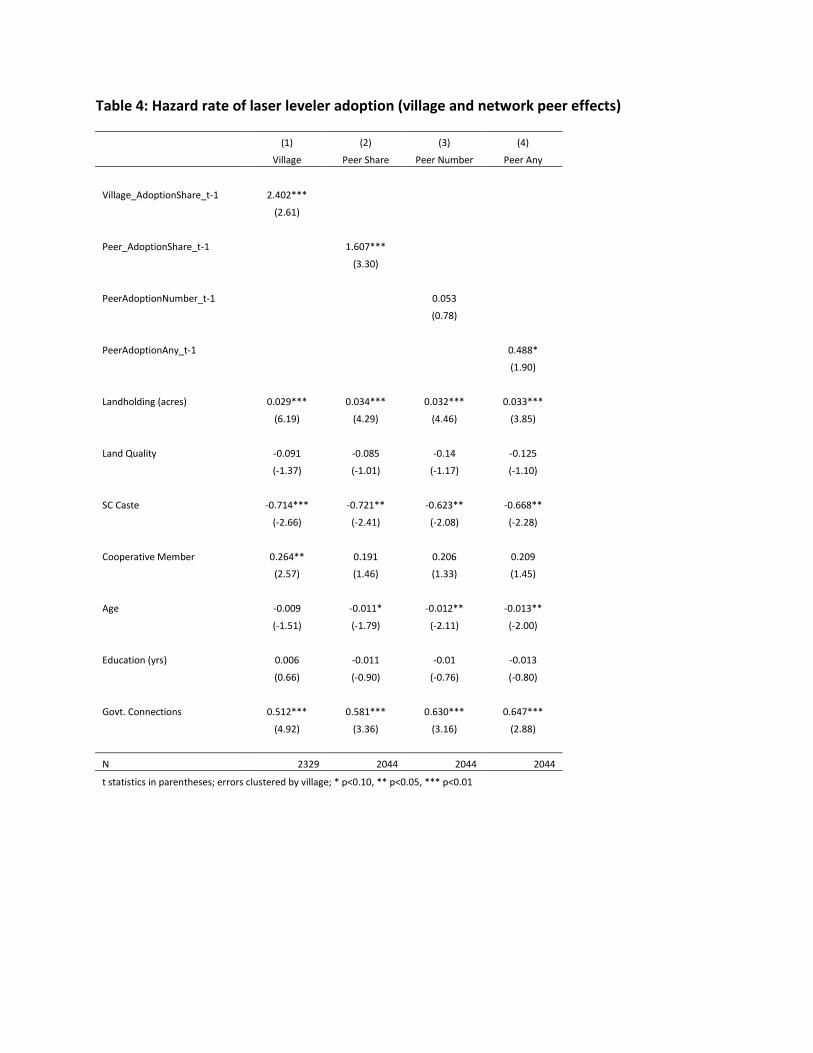
Table 4: Hazard rate of laser leveler adoption (village and network peer effects)
(1) (2) (3) (4)
Village Peer Share Peer Number Peer Any
Village_AdoptionShare_t-1 2.402***
(2.61)
Peer_AdoptionShare_t-1
1.607***
(3.30)
PeerAdoptionNumber_t-1
0.053
(0.78)
PeerAdoptionAny_t-1
0.488*
(1.90)
Landholding (acres) 0.029*** 0.034*** 0.032*** 0.033***
(6.19) (4.29) (4.46) (3.85)
Land Quality -0.091 -0.085 -0.14 -0.125
(-1.37) (-1.01) (-1.17) (-1.10)
SC Caste -0.714*** -0.721** -0.623** -0.668**
(-2.66) (-2.41) (-2.08) (-2.28)
Cooperative Member 0.264** 0.191 0.206 0.209
(2.57) (1.46) (1.33) (1.45)
Age -0.009 -0.011* -0.012** -0.013**
(-1.51) (-1.79) (-2.11) (-2.00)
Education (yrs) 0.006 -0.011 -0.01 -0.013
(0.66) (-0.90) (-0.76) (-0.80)
Govt. Connections 0.512*** 0.581*** 0.630*** 0.647***
(4.92) (3.36) (3.16) (2.88)
N 2329 2044 2044 2044
t statistics in parentheses; errors clustered by village; * p<0.10, ** p<0.05, *** p<0.01

Table 5: Hazard rate of laser leveler adoption (with village fixed effects)
(1) (2) (3) (4)
Village Peer Share Peer
Number Peer Any
Village_AdoptionShare_t-1 -3.133
(-1.36)
Peer_AdoptionShare_t-1
1.100***
(3.40)
PeerAdoptionNumber_t-1
-0.032
(-0.54)
PeerAdoptionAny_t-1
0.413**
(2.07)
Landholding (acres) 0.028*** 0.029*** 0.028*** 0.027***
(8.36) (7.34) (7.66) (6.41)
Land Quality -0.056*** -0.009 -0.040*** -0.038***
(-6.66) (-0.36) (-8.07) (-3.53)
SC Caste -0.743*** -0.800*** -0.749*** -0.771***
(-2.65) (-2.71) (-2.60) (-2.68)
Cooperative Member 0.317*** 0.243*** 0.316*** 0.278***
(8.12) (5.54) (15.74) (10.26)
Age -0.006 -0.006 -0.006 -0.006
(-0.75) (-0.70) (-0.67) (-0.66)
Education (yrs) 0.02 0.014 0.02 0.018
(1.25) (0.94) (1.12) (1.09)
Govt. Connections 0.375*** 0.404*** 0.404*** 0.391***
(5.46) (7.62) (7.25) (5.49)
Village 2 1.660*** 1.048*** 1.194*** 1.192***
(3.85) (14.16) (69.62) (20.54)
Village 3 -0.201 0.367*** 0.211*** 0.384***
(-1.40) (10.13) (4.08) (4.13)
Village 4 -0.521** 0.215** -0.027 0.16
(-2.31) (2.38) (-0.17) (1.21)
Village 5 -2.122*** -0.738*** -1.098*** -0.892***
(-2.78) (-4.79) (-4.56) (-5.36)
N 2329 2044 2044 2044 t statistics in parentheses; errors clustered by village; * p<0.10, ** p<0.05, *** p<0.01

Table 6: Adoption with both village and network effects
(1) (2) (3)
Village + Peer Share Village + Peer Any Peer Share + Any
Village_AdoptionShare_t-1 1.09 2.098**
(1.40) (2.38)
Peer_AdoptionShare_t-1 1.367***
0.980***
(4.57)
(3.18)
PeerAdoptionAny_t-1
0.381* 0.179
(1.83) (0.91)
Landholding (acres) 0.033*** 0.031*** 0.029***
(4.99) (4.85) (7.13)
Land Quality -0.072 -0.09 -0.012
(-1.11) (-1.27) (-0.51)
SC Caste -0.737** -0.714** -0.807***
(-2.54) (-2.57) (-2.73)
Cooperative Member 0.227** 0.269*** 0.239***
(2.05) (3.02) (6.05)
Age -0.01 -0.01 -0.006
(-1.64) (-1.58) (-0.68)
Education (yrs) -0.005 -0.001 0.014
(-0.52) (-0.05) (0.93)
Govt. Connections 0.541*** 0.543*** 0.399***
(4.20) (4.13) (6.64)
Village 2
1.067***
(11.85)
Village 3
0.416***
(4.54)
Village 4
0.253*
(1.95)
Village 5
-0.715***
(-4.14)
N 2044 2044 2044 t statistics in parentheses; errors clustered by village; * p<0.10, ** p<0.05, *** p<0.01

Table 7: Hazard rate of adoption with monthly data
(1) (2) (3)
Peer Share Peer Any Share + Any
Peer_AdoptionShare_t-1 -0.105
-0.486*
(-0.36)
(-1.73)
PeerAdoptionAny_t-1
0.327*** 0.489***
(3.28) (6.30)
Landholding (acres) 0.026*** 0.028*** 0.026***
(7.33) (6.45) (5.97)
Land Quality -0.011 -0.025*** -0.021
(-0.29) (-2.64) (-0.61)
SC Caste -0.792*** -0.816*** -0.823***
(-2.97) (-2.63) (-2.87)
Cooperative Member 0.278*** 0.319*** 0.265***
(4.37) (8.15) (4.25)
Age -0.007 -0.006 -0.007
(-0.85) (-0.69) (-0.80)
Education (yrs) 0.023 0.024 0.024
(1.28) (1.22) (1.26)
Govt. Connections 0.505*** 0.382*** 0.497***
(10.35) (5.11) (8.75)
Village 2 1.541*** 1.278*** 1.580***
(16.65) (18.77) (17.38)
Village 3 -0.484*** -0.646*** -0.243***
(-5.59) (-8.59) (-2.94)
Village 4 -0.711*** -0.920*** -0.501***
(-4.62) (-7.09) (-3.38)
Village 5 -1.827*** -1.953*** -1.659***
(-7.87) (-9.50) (-6.84)
N 21675 22055 21675
t statistics in parentheses; errors clustered by village; * p<0.10, ** p<0.05, *** p<0.01

Table 8: Peer effects by type of relationship
(1) (2) (3) (4) (5) (6) Relative Friend Spoken to Neighbor Knowledgable All
PeerAdoptionAny_t-1 0.320*** 0.372*** 0.341*** 0.327*** 0.424* 0.553*
(2.69) (4.61) (3.51) (3.19) (1.90) (1.86)
RelativeAny_t-1 0.03
0
(0.15)
0.00
FriendAny_t-1
-0.131
-0.188
(-0.82)
(-1.09)
SpokenAny_t-1
-0.110***
-0.152***
(-4.12)
(-3.88)
NeighborAny_t-1
0.001
-0.028
(0.01)
(-0.18)
KnowledgableAny_t-1
-0.173 -0.244
(-0.60) (-0.75)
Landholding (acres) 0.028*** 0.027*** 0.028*** 0.028*** 0.028*** 0.028***
(6.64) (5.84) (6.57) (6.35) (6.70) (6.56)
Land Quality -0.026*** -0.029*** -0.032*** -0.025* -0.007 -0.013
(-3.81) (-4.30) (-3.92) (-1.78) (-0.21) (-0.28)
SC Caste -0.818*** -0.820*** -0.837*** -0.815*** -0.782*** -0.813***
(-2.84) (-2.75) (-2.76) (-2.72) (-3.00) (-4.00)
Cooperative Member 0.317*** 0.322*** 0.325*** 0.319*** 0.312*** 0.320***
(9.72) (8.85) (6.99) (8.42) (7.44) (9.15)
Age -0.006 -0.006 -0.006 -0.006 -0.006 -0.006
(-0.67) (-0.68) (-0.69) (-0.71) (-0.71) (-0.68)
Education (yrs) 0.024 0.026 0.025 0.024 0.022 0.026
(1.08) (1.43) (1.28) (1.18) (1.25) (1.27)
Govt. Connections 0.384*** 0.380*** 0.375*** 0.382*** 0.382*** 0.373***
(4.77) (5.14) (5.13) (4.77) (5.08) (4.87)
Village 2 1.266*** 1.260*** 1.279*** 1.278*** 1.274*** 1.246***
(9.44) (16.23) (18.61) (18.37) (20.68) (7.85)
Village 3 -0.653*** -0.650*** -0.638*** -0.645*** -0.666*** -0.675***
(-11.19) (-8.42) (-8.55) (-9.55) (-6.99) (-7.97)
Village 4 -0.922*** -0.931*** -0.910*** -0.920*** -0.941*** -0.956***
(-8.11) (-7.42) (-7.07) (-7.86) (-5.84) (-6.66)
Village 5 -1.949*** -1.993*** -1.954*** -1.953*** -1.985*** -2.065***
(-8.48) (-9.74) (-9.56) (-11.14) (-7.96) (-7.15)
N 22055 22055 22055 22055 22055 22055 t statistics in parentheses; errors clustered by village; * p<0.10, ** p<0.05, *** p<0.01

Table 9: Hazard rate of adoption, by landholding size
(1) (2) (3)
Small Medium Large
PeerAdoptionAny_t-1 0.419*** 0.423 0.349**
(3.36) (1.38) (2.02)
Landholding (acres) 0.156 0.097*** 0.006
(1.21) (4.03) (1.21)
Land Quality -0.165 -0.186 0.085
(-0.67) (-1.34) (0.67)
SC Caste -1.039** -0.132
(-2.17) (-1.53)
Cooperative Member 0.172 -0.033 -0.052
(0.81) (-0.12) (-0.21)
Age -0.003 -0.001 -0.013
(-0.20) (-0.14) (-0.84)
Education (yrs) -0.006 0.036*** 0.025
(-0.17) (5.36) (0.42)
Govt. Connections 0.397 0.714*** -0.029
(1.43) (3.30) (-0.11)
Village 2 1.061*** 22.035 1.007***
(6.83) . (3.48)
Village 3 -2.041*** 20.614*** -1.209***
(-5.22) (46.66) (-10.91)
Village 4 -2.370*** 20.106*** -1.216***
(-14.63) (48.66) (-4.47)
Village 5 -3.709*** 19.487*** -1.121***
(-31.35) (45.44) (-3.14)
N 11162 7121 3772
t statistics in parentheses; errors clustered by village; * p<0.10, ** p<0.05, *** p<0.01

Table 10: Beliefs about benefits of laser leveling
Believe benefit for:
Crop yield Irrigation time Water savings Weeding time Labor savings
Adopters Yes 95% 100% 100% 34% 49%
No 5% 0% 0% 66% 51%
Don't know 0% 0% 0% 0% 0%
Non-adopters Yes 86% 96% 96% 31% 35%
No 8% 1% 1% 61% 57%
Don't know 6% 4% 3% 8% 8%
(Note: numbers may not add to 100% due to rounding.)
Table 11: Reported changes in inputs and outputs after laser leveling
Rice Yield Wheat Yield Diesel (ltrs) Labor (hrs) Average % change 12.30% 12.10% -25.40% -27.40%
Change at 10th percentile 3.80% 0% -18.80% -12.50% Change at 90th percentile 22.20% 22.20% -33.30% -40.00%
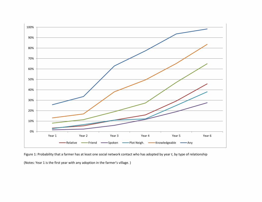
Figure 1: Probability that a farmer has at least one social network contact who has adopted by year t, by type of relationship
(Notes: Year 1 is the first year with any adoption in the farmer’s village. )
0%
10%
20%
30%
40%
50%
60%
70%
80%
90%
100%
Year 1 Year 2 Year 3 Year 4 Year 5 Year 6
Relative Friend Spoken Plot Neigh. Knowledgeable Any

Figure 2: Detecting Influential People in the Village

Figure 3: Friends: Several Components are observed. Critical Nodes that link the widest network are identified.

Figure 4: Contacts: People Whom the Respondents talk with more than others

Figure 5: Network – Most prominent Farmers Sarhal Mandi

Degree Centrality Histogram
Node Count
Range In-Degree .000 - .002 245 .002 - .004 21 .004 - .006 0 .006 - .008 6 .008 - .010 0 .010 - .012 2 .012 - .014 0 .014 - .016 0 .016 - .018 1 .018 - .020 0 > 0.020 9
DISTRIBUTION OF DEGREE CENTRALITY SCORES
MEASURES VALUE
In-Degree Centrality Out-Degree Centrality
MEAN 0.002 0.002 STD.DEV. 0.013 0.004
MIN. 0 0
MAX. 0.141 0.018

Center View

Figure 6: Network – Most prominent Farmers Giddar Pindi

Degree Centrality Histogram
Node Count
Range In-Degree .000 - .002 245 .002 - .004 39 .004 - .006 31 .006 - .008 0 .008 - .010 12 .010 - .012 4 .012 - .014 0 .014 - .016 2 .016 - .018 2 .018 - .020 0 > 0.020 9
DISTRIBUTION OF DEGREE CENTRALITY SCORES
MEASURES VALUE
In-Degree Centrality Out-Degree Centrality
MEAN 0.003 0.003 STD.DEV. 0.01 0.004 MIN. 0 0
MAX. 0.105 0.012

Center View

Figure 7: Network – Most prominent Farmers Khalra

Degree Centrality Histogram
Node Count
Range In-Degree .000 - .002 332
.002 - .004 30 .004 - .006 16 .006 - .008 5 .008 - .010 7 .010 - .012 0 .012 - .014 3 .014 - .016 0 .016 - .018 1 .018 - .020 4 > .020 9
DISTRIBUTION OF DEGREE CENTRALITY SCORES
MEASURES VALUE
In-Degree Centrality Out-Degree Centrality
MEAN 0.002 0.002 STD.DEV. 0.009 0.004 MIN. 0 0
MAX. 0.116 0.017


Designed by soapbox.
The International Growth Centre (IGC) aims to promote sustainable growth in developing countries by providing demand-led policy advice based on frontier research.
Find out more about our work on our website www.theigc.org
For media or communications enquiries, please contact [email protected]
Subscribe to our newsletter and topic updates www.theigc.org/newsletter
Follow us on Twitter @the_igc
Contact us International Growth Centre, London School of Economic and Political Science, Houghton Street, London WC2A 2AE