Adjustment and Application of Transition Matrices in Credit Risk Models
27
Working Paper Adjustment and Application of Transition Matrices in Credit Risk Models This draft: September 2003 Universit¨ at Karlsruhe (TH) Fakult¨ at f¨ ur Wirtschaftswissenschaften Lehrstuhl f¨ ur Statistik, ¨ Okonometrie und Mathematische Finanzwirtschaft Stefan Tr¨ uck and Emrah ¨ Ozturkmen A revised version of this paper will appear in Rachev (ed), Handbook: Computational and Numerical Methods in Finance, to appear in Birkhauser 2004
-
Upload
ernesto-moreno -
Category
Documents
-
view
225 -
download
2
description
Abstract. The paper gives a survey on recent developments on the use of numericalmethods in rating based Credit Risk Models. Generally such modelsuse transition matrices to describe probabilities from moving from one ratingstate to the other and to calculate Value-at-Risk figures for portfolios. Weshow how numerical methods can be used to find so-called true generator matricesin the continuous-time approach, adjust transition matrices or estimateconfidence bounds for default and transition probabilities.
Transcript of Adjustment and Application of Transition Matrices in Credit Risk Models

Working Paper
Adjustment and Application of TransitionMatrices in Credit Risk Models
This draft: September 2003
Universitat Karlsruhe (TH)Fakultat fur Wirtschaftswissenschaften
Lehrstuhl fur Statistik, Okonometrie und MathematischeFinanzwirtschaft
Stefan Truck and Emrah Ozturkmen
A revised version of this paper will appear in Rachev (ed), Handbook:Computational and Numerical Methods in Finance, to appear in
Birkhauser 2004

ADJUSTMENT AND APPLICATION OF TRANSITION
MATRICES IN CREDIT RISK MODELS
STEFAN TRUCK AND EMRAH OZTURKMEN
Abstract. The paper gives a survey on recent developments on the use of nu-
merical methods in rating based Credit Risk Models. Generally such models
use transition matrices to describe probabilities from moving from one rating
state to the other and to calculate Value-at-Risk figures for portfolios. We
show how numerical methods can be used to find so-called true generator ma-
trices in the continuous-time approach, adjust transition matrices or estimate
confidence bounds for default and transition probabilities.
1. Introduction
Borrowing and lending money have been one of the oldest financial transactions.They are the core of the modern world‘s sophisticated economy, providing fundsto corporates and income to households. Nowadays, corporates and sovereign en-tities borrow either on the financial markets via bonds and bond-type products orthey directly borrow money at financial institutions such as banks and savings as-sociations. The lenders, e.g banks, private investors, insurance companies or fundmanagers are faced with the risk that they might lose a portion or even all of theirmoney in case the borrower cannot meet the promised payment requirements.In recent years, to manage and evaluate Credit Risk for a portfolio especially so-
called rating based systems have gained more and more popularity. These systemsuse the rating of a company as the decisive variable and not - like the formerly usedso-called structural models the value of the firm - when it comes to evaluate thedefault risk of a bond or loan. The popularity is due to the straightforwardness ofthe approach but also to the upcoming ”New Capital Accord” of the Basel Com-mittee on Banking Supervision, a regulatory body under the Bank of InternationalSettlements, publicly known as Basel II. Basel II allows banks to base their capitalrequirement on internal as well as external rating systems. Thus, sophisticatedcredit risk models are being developed or demanded by banks to assess the riskof their credit portfolio better by recognizing the different underlying sources ofrisk. Default probabilities for certain rating categories but also the probabilities formoving from one rating state to another are important issues in such Credit RiskModels. We will start with a brief description of the main ideas of rating-basedCredit Risk Models and then give a survey on numerical methods that can be ap-plied when it comes to estimating continous time transition matrices or adjustingtransition probabilities.
Key words and phrases. Credit Risk, Transition Matrix, Bootstrapping.
1

2 STEFAN TRUCK AND EMRAH OZTURKMEN
Table 1. An example for Moody’s one-year transition matrix
Initial Rating at year-end (%)Rating Aaa Aa A Baa Ba B Caa DefaultAaa 93.40 5.94 0.64 0 0.02 0 0 0Aa 1.61 90.55 7.64 0.26 0.09 0.01 0 0.02A 0.07 2.28 92.44 4.63 0.45 0.12 0.01 0Baa 0.05 0.26 5.51 88.48 4.76 0.71 0.08 0.15Ba 0.02 0.05 0.42 5.16 86.91 5.91 0.24 1.29B 0 0.04 0.13 0.54 6.35 84.22 1.91 6.81Caa 0 0 0 0.62 2.05 4.08 69.20 24.06
2. Rating Based Credit Risk Models
2.1. Reduced Form Models - the beginning. In 1994, Jerome S. Fons, was thefirst to develop a so-called reduced form model and to derive credit spreads usinghistorical default rates and recovery rate estimates. Before that most models werebased on the so-called structural approach developed by Merton (1974) calculatingdefault probabilities and credit spreads using the value of the company as thedecisive variable. However, in the model developed by Fons, calculating the priceof credit risk the decisive variables were the rating of a company and historicaldefault probabilities for rating classes and not the value of the firm. Althoughhis approach is rather simple in relation to other theoretical models of credit risk,the predicted credit spreads derived by Fons showed strong similarity towards realmarket data.However, not only the ’worst case’ event of default has influence on the price of
a bond, but also a change in the rating of a company or an issued bond. Therefore,refining Fons model, Jarrow, Lando, Turnbull (JLT)1 introduced a discrete-timeMarkovian Model to estimate changes in the price of loans and bonds. They incor-porate possible rating upgrade, stable rating and rating downgrade (with defaultas a special event) in the reduced form approach. To determine the price of creditrisk both historical default rates and a transition matrix (an exemplary historicaltransition matrix is shown in Table 1) is used.
2.2. Rating Models - the JLT model. Deterioration or improvement in thecredit quality of the issuer is highly important for example if someone wants tocalculate VaR figures for a portfolio or evaluate credit derivatives like credit spreadoptions whose payouts depend on the yield spreads that are influenced by suchchanges. One common way to express these changes in the credit quality of marketparticipants is to consider the ratings given by agencies like Standard & Poors andMoody‘s. Downgrades or upgrades by the rating agencies are taken very seriouslyby market players to price bonds and loans, thus effecting the risk premium andthe yield spreads.Jarrow/Lando/Turnbull (JLT) in 1997 constructed a model that considers dif-
ferent credit classes characterized by their ratings and allows moving within theseclasses. In this section, we will describe the basic idea of the the JLT model andalso some of the extensions by Lando (1998).
1 JLT

ADJUSTMENT AND APPLICATION OF TRANSITION MATRICES IN CREDIT RISK MODELS3
To ease the understanding and interpret the outcomes better, we first focus onthe theoretical framework in the discrete time before going to the continuous timecase.
2.3. The Discrete Time Case. JLT model default and transition probabilitiesby using a discrete time, time-homogenous Markov chain on a finite state spaceS={1,......,K}. The state space S represents the different rating classes. While1 is for the best credit rating, K represents the default case. Hence, the (KxK)one-period transition matrix is:
(2.1) P =
p11 p12 · · · p1Kp21 p12 · · · p2K· · · · · · · · · · · ·pK−1,1 pK−1,2 · · · pK−1,K0 0 · · · 1
where pij ≥ 0 for all i, j, i 6= j, and pii ≡ 1 -∑K
j=1
j 6=ipij for all i. pij represents the
actual probability of going to state j from state i in one time step.
JLT make the following key assumptions underlying their model45:
• The interest rates and the default process are independent under the mar-tingale measure Q.
• The transition matrix is time-homogenous, i.e. we use the same matrix foreach point in time.
• The default state is an absorbing state, represented by pKi = 0 for i =1, · · · ,K − 1 and pKK = 1.
The multi-period transition matrix equals to:
P0,n = Pn
Under the martingale measure the one-period transition matrix equals to:
(2.2) Qt,t+1 =
q11(t, t+ 1) q12(t, t+ 1) · · · q1K(t, t+ 1)q21(t, t+ 1) q22(t, t+ 1) · · · q2K(t, t+ 1)· · · · · · · · · · · ·qK−1,1(t, t+ 1) qK−1,2(t, t+ 1) · · · qK−1,K(t, t+ 1)0 0 · · · 1
where qij(t, t+1) ≥ 0, for all i,j, i 6= j, qij(t, t+1) ≡ 1−∑K
j=1
j 6=iqij , and qij(t, t+1) > 0
if and only if qij > 0 for 0 ≤ t ≤ τ − 1.
JLT argue that, without additional restrictions, the martingale probabilitiesqij(t, t+ 1) can depend on the entire history up to time, i.e. the Markov propertyis not satisfied anymore. Therefore, they assume that the martingale probabilitiesqij(t, t+ 1) satisfy the following equation:
(2.3) qij(t, t+ 1) = πi(t)pij
for all i,j, i 6= j where πi(t) is a deterministic function of time.
45 The assumptions of complete markets with no arbitrage opportunities, thus existence and
uniqueness of the martingale measure Q is a key assumption of all intensity models that will
not be mentioned further during the rest of chapter.

4 STEFAN TRUCK AND EMRAH OZTURKMEN
Differently speaking, given a current state i, the martingale probabilities to movefrom state i to j are proportional to the actual probabilities and the proportionalityfactor depends on time and the current state i, but not on the next state j. JLTcall this factor the risk premium.
We can write the equation (3.17) also in matrix form:
(2.4) Qt,t+1 − I = Π(t)[P − I]
where I is the (KxK) identity matrix and Π(t) = diag(π1(t), . . ., πK−1(t), 1) is a(KxK) diagonal matrix. Given the time dependence of the risk premium, one getsa time-inhomogenous Markov chain under the martingale measure.Often in practise market prices of defaultable claims do not reflect historical
default or transition probabilities. We will see later how with the help of numericalmethods risk premiums can be calculated so historical transition matrices can betransformed into e.g. a one-year transition matrix under the martingale measure.But first, having outlined the basic ideas of the JLT model, we will now describe
the continuous-time case. We will see later that using the continuous approach tocalculate transition and default probabilities has some advantages.
2.4. The Continuous-Time Case. A continuous-time, time-homogenous Markovchain is specified via the (KxK) generator matrix:
(2.5) Λ =
λ11 λ12 · · · λ1Kλ21 λ22 · · · λ2K· · · · · · · · · · · ·λK−1,1 λK−1,2 · · · λK−1,K0 0 · · · 0
where λij ≥ 0, for all i, j and λii = −∑K
j=1
j 6=iλij , for i = 1,.....K. The off-diagonal
elements represent the intensities of jumping to rating j from rating i. The defaultstate K is an absorbing one.The (KxK) t-period transition matrix under the actual probabilities is then given
by
(2.6) P (t) = etΛ =∞∑
k=0
(tΛ)k
k!= I + (tΛ) +
(tΛ)2
2!+(tΛ3)
3!+ · · ·
For example consider the transition matrix
P A B DA 0.90 0.08 0.02B 0.1 0.80 0.1D 0 0 1
then the corresponding generator matrix is
Λ A B DA -0.1107 0.0946 0.0162B 0.1182 -0.2289 0.1107C 0 0 0.
Similar to their discrete-time framework, they transform the empirical generatormatrix to a risk-neutral generator matrix by multiplying it with the risk premium

ADJUSTMENT AND APPLICATION OF TRANSITION MATRICES IN CREDIT RISK MODELS5
matrix, i.e. adjustments of risk to transform the actual probabilities into the risk-neutral probabilities for valuation purposes:
(2.7) Λ(t) ≡ U(t)Λ(t)
where U(t) = diag(µ1(t), · · · , µK−1(t), 1) is a (KxK) diagonal matrix whose firstK-1 entries are strictly positive deterministic functions of t.Thus, JLT define a methodology to value risky bonds as well as credit derivatives
based on ratings allowing changes in credit quality before default. In the followingsection we will give a brief outline on the advantages of continuous modeling versusdiscrete time models.
2.5. Continuous vs. discrete time modeling. Lando/Skodeberg (2000) andLando/Christensen (2002) focus in their papers on the advantages of the continuoustime modeling over the discrete time approach used by rating agencies to analyzerating transition data. Generally, by rating agencies transition probabilities areestimated using the multinomial method by computing
(2.8) pij =Nij
Ni
for j 6= i and where Ni is the number of firms in rating class i at the beginning ofthe year and Nij is the number of firms that migrated to rating class j.The authors argue that these transition probabilities do not capture rare events
such as a transition from AAA to default as they may not be observed. However, itis possible that a firm reaches default through subsequent downgrades from AAA -even within one year, i.e. the probability of moving from AAA to default must benon-zero. Therefore, they purpose the continuous-time method by first estimatingthe generator matrix via the maximum-likelihood estimator:2
(2.9) λij =Nij(T )∫ T0
Yi(s)ds
where Yi(s) is the number of firms in rating class i at time s and Nij(T ) is thetotal number of transitions over the period from i to j, where i 6= j. Under theassumption of time-homogeneity the transition matrix can be computed by theformula P (t) = etΛ.Consider the following example taken from Lando/Skodeberg. There are three
rating classes A, B and D for default. Assume that at the beginning of the yearthere are 10 firms in A and 10 in B and none in default. Suppose that one A-rated company is downgraded to B after one month and stays there for the rest ofthe year; a B-rated company is upgraded to A after two months to remain therefor the rest of the period and a B-rated company defaults after six months. Thediscrete-time multinomial method then estimates the following one-year transitionmatrix:
P A B DA 0.90 0.10 0B 0.1 0.80 0.1D 0 0 1
The maximum-likelihood estimator for the continuous-time approach computes thefollowing generator matrix first:
2 See Kuchler and Sorensen [1997] for details.

6 STEFAN TRUCK AND EMRAH OZTURKMEN
Λ A B DA -0.10084 0.10084 0B 0.10909 -0.21818 0.10909D 0 0 0
For instance, the non-diagonal element λAB equals to:
λAB =NAB(1)∫ 1
0YA(s)ds
=1
9 + 112 +
1012
= 0.10084
The diagonal element λAA is computed so that the row sums to zero. Exponenti-ating the generator gives the following one-year transition matrix:
P A B DA 0.90887 0.08618 0.00495B 0.09323 0.80858 0.09819D 0 0 1
Thus, we have a strictly positive default probability for class A although there havebeen no observation from A to default in this period. However, this makes sense asthe migration probability from A to B and from B to default are non-zero. Thus,it could happen within one year that a company is downgraded from rating stateA to B and then defaults being in rating state B.Before we go to the time-inhomogenous case let us briefly summarize the key
advantages of the continuous time approach:3
• We can get non-zero estimates for probabilities of rare events which themultinomial method estimates to be zero.
• We can obtain transition matrices for arbitrary time horizons.• We have a good method to assess the proposal of Basel-2 to impose aminimum probability of 0.03% for events that are estimated with a binomialor multinomial method to have a zero probability.
• In the continous-time approach we do not have to worry which yearly peri-ods we consider. Using a discrete time approach may lead to quite differentresults depending on the starting point of our consideration.
• The continuous framework permits of generating confidence sets as dis-cussed in later sections.
• The dependence on covariates can be tested and business cycles effects canbe quantified.
For the time-inhomogeneous case, the Nelson-Aalen estimator is used:
λhj(t) =∑
{k:Thjk≤t}
1
Yh(Thjk)
where Thj1 < Thj2 < . . . are the observed times of transitions from h to j and Yh(t)counts the number of firms in rating class h at time just prior to t. The transitionmatrix is then computed as follows:
(2.10) P (s, t) =
m∏
i=1
(I +∆Λ(T ))
3 See Lando/Skodeberg [2000] p.2ff. and Lando/Christensen [2002] p.2ff.

ADJUSTMENT AND APPLICATION OF TRANSITION MATRICES IN CREDIT RISK MODELS7
where I is the identity matrix, Ti is a jump time in the interval ]s,t] and
∆Λ(T ) =
−∆N1(Ti)Y1(Ti)
−∆N12(Ti)Y1(Ti)
· · · −∆N1K(Ti)Y1(Ti)
−∆N21(Ti)Y2(Ti)
−∆N2(Ti)Y2(Ti)
· · · −∆N2K(Ti)Y2(Ti)
· · · · · · · · · · · ·−∆NK−1,1(Ti)
YK−1(Ti)−∆NK−1,2(Ti)
YK−1(Ti)· · · −∆NK−1,K(Ti)
YK−1(Ti)
0 0 · · · 0
The diagonal elements count the total number of transitions away from class idivided by the number of exposed firms and the off-diagonal elements count thenumber of migration to the corresponding class, again divided by the number offirms exposed. This estimator can be interpreted a cohort method applied to veryshort intervals.Implementing this approach to our example we obtain the following matrices:
∆Λ(T 1
12
) =
−0.1 0.1 00 0 00 0 0
∆Λ(T 2
12
) =
0 0 0111 − 1
11 00 0 0
∆Λ(T 6
12
) =
0 0 00 −0.1 0.10 0 0
Using equation 2.5 we get
P (0, 1) =
0.90909 0.08181 0.009090.09091 0.81818 0.090910 0 1
As in the time-homogeneous case we obtain strictly positive default probabilityfor class A although the entries in the matrix above are slightly different than in thetime-homogenous case. However, Lando and Skodeberg indicate that in most casesthe results are not dramatically different for large data sets. However, comparedto the estimator for the transition matrix using the discrete multinomial estimatorwe get quite different results.
3. Finding Generator Matrices for Markov chains
So far we described the basic ideas of rating based credit risk evaluation methodsand the advantages of continuous time transition modeling over the discrete timecase.Despite these advantages of continuous modeling, there are also some problems
to deal with like the existence, uniqueness or adjustment of the generator matrixto the corresponding discrete transition matrix.An important issue when dealing with the continuous time approach is whether
for a given discrete one-year transition matrix a so-called true generator exists.For some discrete transition matrices there does not exist a generator matrix whilefor some though there exists a generator, it has negative off-diagonal elements.This would mean that considering short time intervals transition probabilities maybe negative what is from practical point of view not acceptable. Examining this

8 STEFAN TRUCK AND EMRAH OZTURKMEN
question and suggesting numerical methods for finding true generators or approx-imations for true generators we will follow an approach by Israel/Rosenthal/Wei(2000).In their paper they first identify conditions under which a true generator does or
does not exist. Then they provide a numerical method for finding the true generatoronce its existence is proved and how to obtain an approximate one in case of theabsence of a true generator.The authors define two issues with transition matrices: Embeddability, which is
to determine if an empirical transition matrix is compatible with a true generatoror a Markov process; and identification, which is to search for the true generatoronce its existence is known.
3.1. Computing the Generator Matrix to a given Transition Matrix.
Given the one-year N ×N transition matrix P we are interested in finding a gen-erator matrix Λ such that:
(3.1) P = eΛ =
∞∑
k=0
Λk
k!= I + Λ+
Λ2
2!+Λ3
3!+ · · ·
Dealing with the question whether there exists a generator matrix for a giventransition matrix P , the first task is to calculate S with
S = max{(a− 1)2 + b2; a+ bi is an eigenvalue of P, a, b ∈ R}where all the (possibly complex) eigenvalues of P are examined by computing
the absolute square of the eigenvalue minus 1 and taking the maximum of these.It can be shown that if the condition S < 1 holds
(3.2) Λ∗ = (P − I)− (P − I)2
2+(P − I)3
3− (P − I)4
4+ · · ·
converges geometrically quickly and is an N×N matrix having row-sums of zeroand satisfying P = eΛ
∗
exactly.4
It is important to note that even if the series Λ∗ does not converge or convergesto a matrix that cannot be a true generator P may still have a true generator.There is also a simpler way to check if S < 1, namely if the transition matrix
consists of diagonal elements that are greater than 0.5. Then S is less than one andthe convergence of is guaranteed. For most transition matrices in practice this willbe true, so we can assume that generators having row-sums of zero and satisfyingP = eΛ
∗
can be found.However, often there remains one problem: The main disadvantage of series 3.2
is that Λ∗ may converge but does not have to be a generator matrix, particularlyit is possible that some off-diagonal elements are negative.We will illustrate this with an example. Consider the one-year transition matrix:
P A B C DA 0.9 0.08 0.0199 0.0001B 0.050 0.850 0.090 0.010C 0.010 0.090 0.800 0.100D 0 0 0 1
Calculating the generator that exactly matches P = eΛ∗
we get with 3.2
4 For proof see Appendix 1 on p.23 in Israel et al.

ADJUSTMENT AND APPLICATION OF TRANSITION MATRICES IN CREDIT RISK MODELS9
Λ A B C DA -0.1080 0.0907 0.0185 -0.0013B 0.0569 -0.1710 0.1091 0.0051C 0.0087 0.1092 -0.2293 0.1114D 0 0 0 0
having a negative entry in λAD.From economic viewpoint this is not acceptable because a negative entry in the
generator may lead for very short time intervals to negative transition probabilities.Israel/Rosenthal/Wei (IRW) show that it is possible that sometimes there existmore than one generator. They provide conditions for the existence or non-existenceof a valid generator matrix and a numerical algorithm for finding a valid generator.
3.2. Conditions for the Existence of a valid Generator. Conditions for
the non-existence of a generator
We will first define the conditions to conclude the non-existence of a generator.If
• det(P ) ≤ 0; or• det(P ) >
∏i pii; or
• there are states i and j such that j is accessible from i, but pij = 0.then there is not a generator matrix exact for P.
Conditions for the uniqueness of a generator
Beside the problem of the existence of the generator matrix, there is also theproblem of its uniqueness, as P sometimes has more than one valid generator. Asit is unlikely for a firm to migrate to a ”far” rating from its current rating, theauthors suggest to choose among valid generators the one with the lowest value of
J =∑
i,j
|j − i||λij |
which ensures that the chance of jumping too far is minimized.A theorem for the uniqueness of the generator is as follows:
• If det(P ) > 0.5, then P has at most one generator.• If det(P ) > 0.5 and ||P − I|| < 0.5, then the only possible generator for Pis ln(P ).
• If P has distinct eigenvalues and det(P ) > e−π, then the only possiblegenerator is log(P ).
For the proofs of the above conditions and further material we refer to the originalarticle.
Conditions for the non-existence of a valid generator
Investigating the existence or non-existence of a valid generator matrix with onlypositive off-diagonal elements we start with another result obtained by Singer andSpilerman (1976):Let P be a transition matrix that has real distinct eigenvalues.
• If all eigenvalues of P are positive, then log(P ) is the only real matrix Λsuch that exp(Λ) = P .

10 STEFAN TRUCK AND EMRAH OZTURKMEN
• If P has any negative eigenvalues, then there is no real matrix Λ such thatexp(Λ) = P .
Using the conditions above we can conclude a condition for the non-existence ofa valid generator.Let P be a transition matrix such that at least one of the following three condi-
tions hold:
• det(P ) > 1/2 and |P − I| < 1/2 or• P has distinct eigenvalues and det(P ) > e−π or• P has distinct real eigenvalues.
Suppose further that the series 3.2 converges to a matrix Λ with negative off-diagonal entries. Then there does not exist a valid generator for P.
In our example we find for
P =
0.9 0.08 0.0199 0.00010.050 0.850 0.090 0.0100.010 0.090 0.800 0.1000 0 0 1
• det(P ) = 0.6015 and |P − I| = 0 ≤ 1/2• P has the distinct positive eigenvalues 0.9702, 0.8529, 0.7269 and 1.0000and det(P ) = 0.6015 > 0.0432 = e−π
• P has distinct real eigenvalues
So all three conditions hold - however, to show that one of the conditions holdswould have been enough - and since the series 3.2 converges to
Λ =
−0.1080 0.0907 0.0185 −0.00130.0569 −0.1710 0.1091 0.00510.0087 0.1092 −0.2293 0.11140 0 0 0
we find that there exists no true generator.
An algorithm to search for a valid generator
Israel et al. also provide a search algorithm for a valid generator if the series3.2 fails to converge, or converges to a matrix that has some negative offdiagonalterms while none of the three conditions above holds. We stated already that it isstill possible that a generator exists even if 3.2 fails to converge.Israel et al. use Lagrange interpolation in their search algorithm. They assume
that P is n × n with distinct eigenvalues e1, e2, ..., en and that there exists anarbitrary function f analytic in a neighborhood of each eigenvalue with f(P ) =g(P ). Here g is the polynomial of degree n− 1 such that g(ej) = f(ej) for each j.Using the Lagrange interpolation formula leads to:
g(x) =∑
j
∏
k 6=j
x− ekej − ek
f(ej)(3.3)
Obviously the product is over all eigenvalues ek except ej and the sum is overall eigenvalues ej .

ADJUSTMENT AND APPLICATION OF TRANSITION MATRICES IN CREDIT RISK MODELS11
To search for generators, the values f(ej) must satisfy
f(ej) = log|ej |+ i(arg(ej) + 2πkj(3.4)
where kj is an arbitrary integer and ej may be a complex number and |ej | =√Re(ej)2 + Im(ej)2 and arg(ej) = arctan(Im(ej)/Re(ej)). In theory, it is possi-
ble to find a generator by checking all branches of the logarithm of ej and usingLagrange interpolation to compute f(P ) for each possible choice of k1, k2, ..., kn.Each time it is checked if the nonnegativity condition of the off-diagonal elementsis satisfied. If P has distinct eigenvalues, then this search is finite, as the followingtheorem shows.
If P has distinct eigenvalues and if λ is a generator for P , then each eigenvalue
e of Q satisfies that |Im(e)| ≤ |ln(det(P ))|. In particular, there are only a finite
number of possible branch values of log(P ) which could possibly be generators of Psince, if det(P ) ≤ 0 then no generator exists.
Thus, due to the finite number of possible branch values of log(P ) whenever Phas distinct eigenvalues, it is possible to construct a finite algorithm to search forall possible generators of P .The necessary algorithm can be described as follows:
• Step 1. Compute the eigenvalues e1, e2, ..., en of P , and verify that they areall distinct.
• Step 2. For each eigenvalue ej , choose an integer kj such that |Imλ| =|arg(ej) + 2πkj | ≤ |ln(det(P ))|.
• Step 3. For the collection of integers k1, k2, ..., kn set f(ej) = log|ej | +i(arg(ej) + 2πkj). Let then g(x) be the function given in 3.3
• Step 4. For g(x) compute the matrix Q = g(P ), and see if it is a validgenerator.
• Step 5. If Q is not a valid generator return to Step 2, modifying one ormore of the integers kj . Continue until all allowable collections k1, k2, ..., knhave been considered.
For the rare cases where repeated eigenvalues are present, the authors refer toSinger and Spilerman 1976.
3.3. Methods for finding Approximations of the Generator. As we sawin the previous section, it is not unlikely that the series 3.2 converges to a gen-erator with negative off-diagonal elements and there exists no generator withoutoff-diagonal elements. Thus, either the calculated generator has to be adjusted orwe have to use different methods to calculate the generator matrix. In the followingsection different methods will be discussed.If we find a generator matrix with negative entries in a row, we will have to
correct this. The result may lead to a generator not providing exactly P = eΛ∗
butonly an approximation, though ensuring that from economic viewpoint the neces-sary condition that all off-diagonal row entries in the generator are non-negative isguaranteed.The literature suggests different methods to deal with this problem if calculating
Λ leads to a generator matrix with negative row entries:

12 STEFAN TRUCK AND EMRAH OZTURKMEN
The Jarrow, Lando, Turnbull Method
Jarrow et al. (1997) suggest a method where every firm is assumed to have madeeither zero or one transition throughout the year. Under this hypothesis it can beshown that for λi 6= 0 for i = 1, . . . ,K − 1
(3.5) exp(Λ) =
eλ1λ12(e
λ1−1)λ1
· · · λ1K(eλ1−1)λ1
λ21(eλ2−1)λ2
eλ2 · · · λ2K(eλ2−1)λ2
· · · · · · · · · · · ·
λK−1,1(eλK−1−1)
λK−1
λK−1,2(eλK−1−1)
λK−1
· · · λK−1,K(eλK−1−1)λK−1
0 0 · · · 1
the estimates of Λ can be obtained by solving the system:
qii = eλi for i = 1, . . . ,K − 1 and
qij = λij(eλi − 1) for i, j = 1, . . . ,K − 1
JLT provide the solution to this system as
λi = log(qii) for i = 1, . . . ,K − 1 and
λij = qij ·log(qii)
(qii − 1)for i 6= j and i, j . . . ,K − 1
This leads only to an approximate generator matrix, however it is guaranteedthat the generator will have no non-negative entries except the diagonal elements.For our example, the JLT method gives the associated approximate generator
Λ A B C DA -0.1054 0.0843 0.0210 0.0001B 0.0542 -0.1625 0.0975 0.0108C 0.0112 0.1004 -0.2231 0.1116D 0 0 0 0
with no-negative entries, however, exp(Λ) is only close to the original transitionmatrix P :
PJLT A B C DA 0.9021 0.0748 0.0213 0.0017B 0.0480 0.8561 0.0811 0.0148C 0.0118 0.0834 0.8041 0.1006D 0 0 0 1
Especially in the last column high deviations (from 0.0001 to 0.0017 in the firstrow or 0.0148 instead of 0.010 in the second) for low default probabilities haveto be considered as a rather rough approximation. We conclude that the methodsuggested by JLT in 1997 solves the problem of negative entries in the generator

ADJUSTMENT AND APPLICATION OF TRANSITION MATRICES IN CREDIT RISK MODELS13
matrix, though we get an approximation that is not really close enough to the ’real’transition matrix.
Methods suggested by Israel, Rosenthal and Wei
Due to the deficiencies of the method suggested by JLT, in their paper IRW sug-gest a different approach to finding an approximate true generator. They suggest,to use 3.2 to calculate the associated generator and then adjusting this matrix usingone of the following methods:
• Replace the negative entries by zero and add the appropriate value backin the corresponding diagonal entry to guarantee that row-sums are zero.Mathematically,
λij = max(λij , 0), j 6= i; λii = λii +∑
j 6=i
min(λij , 0)
The new matrix will not exactly satisfy P = eΛ∗
.• Replace the negative entries by zero and add the appropriate value back intoall entries of the corresponding row proportional to their absolute values.Let Gi be the sum of the absolute values of the diagonal and nonnegativeoff-diagonal elements and Bi the sum of the absolute values of the negativeoff-diagonal elements:
Gi = |λii|+∑
j 6=i
max(λij , 0); Bi =∑
j 6=i
max(−λij , 0)
Then set the modified entries
λij =
0, i 6= j and λij < 0
λij − Bi|λij |Gi
otherwise ifGi > 0
λij , otherwise ifGi = 0
In our example where the associated generator was
Λ A B C DA -0.1080 0.0907 0.0185 -0.0013B 0.0569 -0.1710 0.1091 0.0051C 0.0087 0.1092 -0.2293 0.1114D 0 0 0 0
applying the first method and setting λAD to zero and adding −0.0013 to thediagonal element λAA we would get for the adjusted generator matrix Λ
∗
Λ∗ A B C DA -0.1093 0.0907 0.0185 0B 0.0569 -0.1710 0.1091 0.0051C 0.0087 0.1092 -0.2293 0.1114D 0 0 0 0
which gives us for the approximate one-year transition matrix:
PIRW1 A B C DA 0.8989 0.0799 0.0199 0.0013B 0.0500 0.8500 0.0900 0.0100C 0.0100 0.0900 0.8000 0.1000D 0 0 0 1.

14 STEFAN TRUCK AND EMRAH OZTURKMEN
Obviously the transition matrix PIRW1 is much closer to the ’real’ one-yeartransition than using the JLT method. Especially for the second and third row weget almost exactly the same transition probabilities than for the ’real’ transitionmatrix. Also the deviation for the critical default probability λAD is clearly reducedcompared to the JLT method described above.Applying the second suggested method and again replacing the negative entries
by zero but ’redistributing’ the appropriate value to all entries of the correspondingrow proportional to their absolute values gives us the adjusted generator
Λ∗ A B C DA -0.1086 0.0902 0.0184 0B 0.0569 -0.1710 0.1091 0.0051C 0.0087 0.1092 -0.2293 0.1114D 0 0 0 0
and the associated one-year transition matrix
PIRW1 A B C DA 0.8994 0.0795 0.0198 0.0013B 0.0500 0.8500 0.0900 0.0100C 0.0100 0.0900 0.8000 0.1000D 0 0 0 1.
Again we get results that are very similar to the ones using the first method byIsrael et al. The authors state that generally by testing various matrices they foundsimilar results. To compare the goodness of the approximation they used differentdistance matrix norms.While the approximation of the method suggested by JLT in their 1997 seminal
paper is rather rough, the methods suggested by IRW give better approximationsif the true transition matrix. In the next section we will now deal with the questionhow to adjust transition matrices according to some conditions derived from marketprices or macro-economic forecasts.
4. Modifying Transition Matrices
4.1. The Idea. Another issue when dealing with transition matrices is to adjust,re-estimate or change the transition matrix due to some economic reason. In thissection we will describe numerical methods that can be applied to modify e.g.historical transition matrices. As we stated before the idea of time-homogenoustransition matrices is often not realistic. Due to changes in the business cycles likerecession or expansion of the economy average transition matrices estimated outof historical data are modified. A well-known approach where transition matriceshave to be adjusted according to the macro-economic situation is the CreditPortfolioView model by the McKinsey Company. A more thorough description of the ideasbehind the model can be found in Wilson (1997). Another issue e.g. described inJLT (1997) is for example to match transition matrices with default probabilitiesimplied in bond prices observed in the market. We will now describe some of themethods mentioned by the literature so far.
4.2. Methods suggested by Lando. Again we consider the continuous-time casewhere the time-homogenous Markov chain is specified via the (KxK) generator

ADJUSTMENT AND APPLICATION OF TRANSITION MATRICES IN CREDIT RISK MODELS15
matrix:
(4.1) Λ =
λ11 λ12 · · · λ1Kλ21 λ22 · · · λ2K· · · · · · · · · · · ·λK−1,1 λK−1,2 · · · λK−1,K0 0 · · · 0
where
λij ≥ 0 for all i, j and
λii = −K∑
j=1
j 6=i
λij for i = 1,.....K.
The off-diagonal elements represent the intensities of jumping to rating j fromrating i. The default state K is an absorbing one. As we already showed in theprevious section using the generator matrix we get the K ×K t-period transitionmatrix by
P (t) = exp(tΛ) =
∞∑
k=0
(tΛ)k
k!(4.2)
In his paper Lando (1999) extends the JLT approach and describes three differentmethods to modify the transition matrices so that the implied default probabilitiesare matched. Assuming a known recovery rate ϕ we can derive the implied survivalprobabilities from the market prices of risky bonds for each rating class
(4.3) Qi0(τ > t) =
vi(0, t)− ϕp(0, t)
(1− ϕ)p(0, t)for i = 1,......K-1
where vi(0, t) is the price of a risky bond with rating and i, p(0, t) is the price of ariskless bond. We can then calculate the one-year implied default probabilities as
(4.4) piK = 1− Qi0(τ > 1)
Based on this prework Lando aims to create a family of transition matrices (Q(0, t))t>1
so that the implied default probabilities for each maturity match the correspondingentries in the last column of Q(0, t). Assuming a given one-year transition matrixP and an associated generator matrix Λ with P = eΛ, he proposes the followingprocedure:
(1) Let Q(0, 0) = I
(2) Given Q(0, t), choose Q(t, t+ 1) such that
Q(0, t)Q(t, t+ 1) = Q(0, t+ 1), where (Q(0, t+ 1))iK = 1− Qi(τ > t+ 1)
for i = 1,.....K-1(3) Go to step 2.
The difference between the methods is how step 2 is performed. It is important tonote that this procedure only matches the implied default probabilities. To matchthe implied migration probabilities, one needs suitable contracts such as creditswaps against downgrade risk with the full maturity spectrum.

16 STEFAN TRUCK AND EMRAH OZTURKMEN
In each step the generator matrix Λ is modified such that
Q(0, 1) = eΛ(0)
Q(1, 2) = eΛ(1)
and they satisfy
Q(0, 1)Q(1, 2) = Q(0, 2)
where Λ(0) is a modification of Λ depending on Π1 = (Π11,Π12,Π13) and Λ(1) isa modification of Λ depending on Π2 = (Π21,Π22,Π23) where Π1 and Π2 have tosatisfy
piK(0, 1) = 1− Q(0, 1)
piK(0, 2) = 1− Q(0, 2)
Note that the generator matrix has to be checked if it still fulfills the criteria, namelynon-negative off-diagonal elements and row sums of zero for each row. Having thegenerator matrix, all we have to do is to exponentiate it to get the transition matrix.To illustrate the methods we will always give an example based on a hypothetical
transition matrix with three possible rating categories {A,B,C} and a default state{D} of the following form. Let’s assume our historical yearly transition matrix hasthe form:
P A B C DA 0.900 0.080 0.017 0.003B 0.050 0.850 0.090 0.010C 0.010 0.090 0.800 0.100D 0 0 0 1
Thus, the associated generator is:
Λ A B C DA -0.1080 0.0909 0.0151 0.0020B 0.0569 -0.1710 0.1092 0.0050C 0.0087 0.1092 -0.2293 0.1114D 0 0 0 0
We further assume that we forecasted (or calculated implied default probabilitiesusing bond prices) the following one-year default probabilities for Rating classes{A,B,C}:
A B CpiK 0.006 0.03 0.2
In the following subsections we will refer to these transition matrices and defaultprobabilities and show adjustment methods for the generator and probability tran-sition matrix.
Modifying default intensities.
The first method we describe modifies the default column of the generator matrixand simultaneously modifies the diagonal element of the generator according to:

ADJUSTMENT AND APPLICATION OF TRANSITION MATRICES IN CREDIT RISK MODELS17
λ1K = π1 · λ1K and λ11 = λ11 − (π1 − 1) · λ1Kλ2K = π2 · λ2K and λ22 = λ22 − (π2 − 1) · λ2K· · · · · ·
and for row K − 1:λK−1,K = πK−1 · λK−1,K and
λK−1,K−1 = λK−1,K−1 − (πK−1 − 1) · λK−1,Ksuch that for the new transition matrix P with
P (t) = exp(tΛ) =∞∑
k=0
(tΛ)k
k!(4.5)
the last column equals the risk-neutral default probabilities estimated from themarket.
P (:;K) =
p1Kp2K· · ·pK−1,K1
(4.6)
Thus, with these modifications Λ is also a generator with rows summing tozero. The modifications are done numerically such that all conditions are matchedsimultaneously.Using numerical solution, we get π1 = 1.7443, π2 = 4.1823, π3 = 2.1170 and thus,
for the modified generator matrix
Λ A B C DA -0.1095 0.0909 0.0151 0.0034B 0.0569 -0.1869 0.1092 0.0209C 0.0087 0.1092 -0.3537 0.2358D 0 0 0 0
and the associated probability transition matrix is:
P A B C DA 0.8987 0.0793 0.0161 0.0060B 0.0496 0.8365 0.0840 0.0300C 0.0094 0.0840 0.7066 0.2000D 0 0 0 1.
We find that due to the fact that the changes in the generator only take placein the last column and in the diagonal elements, for the new probability transitionmatrix most of the probability mass is shifted from the default probability to thediagonal element - especially when the new (calculated) default probability is sig-
nificantly higher. Still, if a jump occurs, interpreting − λijλiias the probability for a
jump into the new rating class j also these probabilities slightly change since λii ismodified. In our case we find that for example for rating class A the conditionalprobability when a jump occurs, to jump to default has increased from 1.8% to morethan 3% the other conditional probabilities slightly decrease from 84% to 83% andfrom 14% to 13.8%. These results are confirmed by taking a look at the other rows

18 STEFAN TRUCK AND EMRAH OZTURKMEN
and also by the associated new one-year transition matrix. We conclude that themain changes only happen in the diagonal element and in the default transition.
Modifying the rows of the generator Matrix
This method goes back to Jarrow, Lando and Turnbull (1997) where again a nu-merical approximation is used to solve the equations. The idea is not only to applythe last column and the diagonal elements of the generator matrix but multiplyingeach row by a factor such that the calculated or forecasted default probabilities arematched.Thus, we get:
(4.7) Λ =
π1 · λ11 π1 · λ12 · · · π1 · λ1Kπ2 · λ21 π2 · λ22 · · · π2 · λ2K· · · · · · · · · · · ·πK−1 · λK−1,1 πK−1 · λK−1,2 · · · πK−1 · λK−1,K0 0 · · · 0
Applying this method and solving
P (t) = exp(tΛ) =
∞∑
k=0
(tΛ)k
k!(4.8)
subject to P (:;K) = (p1K , p2K , · · · , pK−1,K , 1) numerically we get for
Λ A B C DA -0.1455 0.1225 0.0204 0.0027B 0.1149 -0.3457 0.2207 0.0101C 0.0198 0.2482 -0.5212 0.2532D 0 0 0 0
and the associated probability transition matrix is:
P A B C DA 0.8706 0.0988 0.0246 0.0060B 0.0926 0.7316 0.1458 0.0300C 0.0247 0.1639 0.6114 0.2000D 0 0 0 1.
In this case due to the different method more probability mass is shifted from thediagonal element of the transition matrix to the others row entries. Considering forexample the new transition matrix we find that for rating state B the probabilityfor staying in the same rating category decreases from 0.85 to approximately 0.73while for all the other row entries the probability significantly increases - e.g. from0.05 to 0.09 for moving from rating state B to rating state A. These results wereconfirmed by applying the method to different transition matrices, so we concludethat the method that modifies the complete row of the generator spreads clearlymore probability mass from the diagonal element to the other elements than thefirst method does. It could be used when the transition matrix should be adjustedto an economy in a rather unstable situation.
Modifying eigenvalues of the transition probability matrix
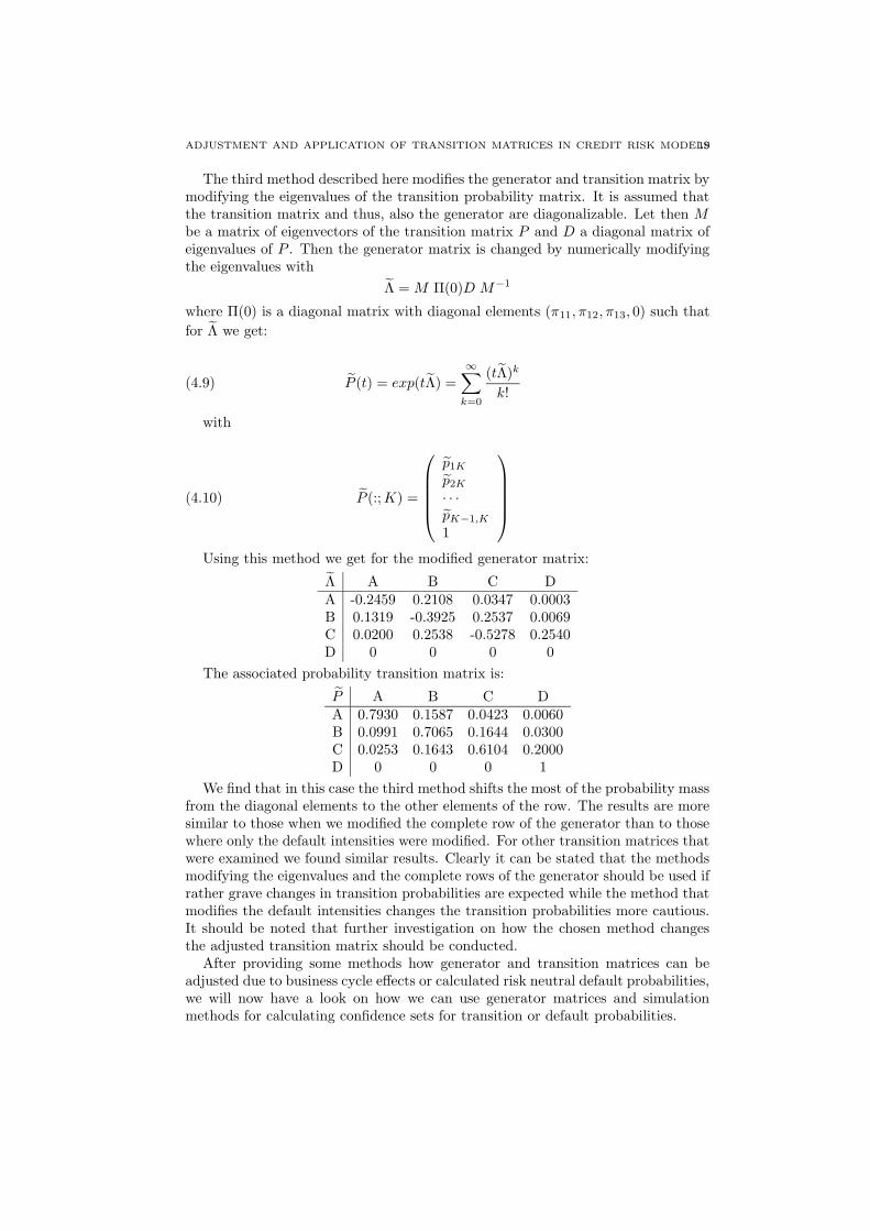
ADJUSTMENT AND APPLICATION OF TRANSITION MATRICES IN CREDIT RISK MODELS19
The third method described here modifies the generator and transition matrix bymodifying the eigenvalues of the transition probability matrix. It is assumed thatthe transition matrix and thus, also the generator are diagonalizable. Let then Mbe a matrix of eigenvectors of the transition matrix P and D a diagonal matrix ofeigenvalues of P . Then the generator matrix is changed by numerically modifyingthe eigenvalues with
Λ =M Π(0)D M−1
where Π(0) is a diagonal matrix with diagonal elements (π11, π12, π13, 0) such that
for Λ we get:
P (t) = exp(tΛ) =
∞∑
k=0
(tΛ)k
k!(4.9)
with
P (:;K) =
p1Kp2K· · ·pK−1,K1
(4.10)
Using this method we get for the modified generator matrix:
Λ A B C DA -0.2459 0.2108 0.0347 0.0003B 0.1319 -0.3925 0.2537 0.0069C 0.0200 0.2538 -0.5278 0.2540D 0 0 0 0
The associated probability transition matrix is:
P A B C DA 0.7930 0.1587 0.0423 0.0060B 0.0991 0.7065 0.1644 0.0300C 0.0253 0.1643 0.6104 0.2000D 0 0 0 1
We find that in this case the third method shifts the most of the probability massfrom the diagonal elements to the other elements of the row. The results are moresimilar to those when we modified the complete row of the generator than to thosewhere only the default intensities were modified. For other transition matrices thatwere examined we found similar results. Clearly it can be stated that the methodsmodifying the eigenvalues and the complete rows of the generator should be used ifrather grave changes in transition probabilities are expected while the method thatmodifies the default intensities changes the transition probabilities more cautious.It should be noted that further investigation on how the chosen method changesthe adjusted transition matrix should be conducted.After providing some methods how generator and transition matrices can be
adjusted due to business cycle effects or calculated risk neutral default probabilities,we will now have a look on how we can use generator matrices and simulationmethods for calculating confidence sets for transition or default probabilities.
20 STEFAN TRUCK AND EMRAH OZTURKMEN
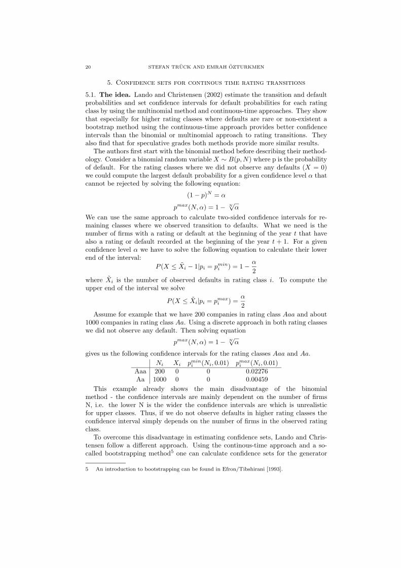
5. Confidence sets for continous time rating transitions
5.1. The idea. Lando and Christensen (2002) estimate the transition and defaultprobabilities and set confidence intervals for default probabilities for each ratingclass by using the multinomial method and continuous-time approaches. They showthat especially for higher rating classes where defaults are rare or non-existent abootstrap method using the continuous-time approach provides better confidenceintervals than the binomial or multinomial approach to rating transitions. Theyalso find that for speculative grades both methods provide more similar results.The authors first start with the binomial method before describing their method-
ology. Consider a binomial random variable X ∼ B(p,N) where p is the probabilityof default. For the rating classes where we did not observe any defaults (X = 0)we could compute the largest default probability for a given confidence level α thatcannot be rejected by solving the following equation:
(1− p)N = α
pmax(N,α) = 1− N√α
We can use the same approach to calculate two-sided confidence intervals for re-maining classes where we observed transition to defaults. What we need is thenumber of firms with a rating or default at the beginning of the year t that havealso a rating or default recorded at the beginning of the year t + 1. For a givenconfidence level α we have to solve the following equation to calculate their lowerend of the interval:
P (X ≤ Xi − 1|pi = pmini ) = 1− α
2
where Xi is the number of observed defaults in rating class i. To compute theupper end of the interval we solve
P (X ≤ Xi|pi = pmaxi ) =
α
2
Assume for example that we have 200 companies in rating class Aaa and about1000 companies in rating class Aa. Using a discrete approach in both rating classeswe did not observe any default. Then solving equation
pmax(N,α) = 1− N√α
gives us the following confidence intervals for the rating classes Aaa and Aa.
Ni Xi pmini (Ni, 0.01) pmax
i (Ni, 0.01)Aaa 200 0 0 0.02276Aa 1000 0 0 0.00459
This example already shows the main disadvantage of the binomialmethod - the confidence intervals are mainly dependent on the number of firmsN, i.e. the lower N is the wider the confidence intervals are which is unrealisticfor upper classes. Thus, if we do not observe defaults in higher rating classes theconfidence interval simply depends on the number of firms in the observed ratingclass.To overcome this disadvantage in estimating confidence sets, Lando and Chris-
tensen follow a different approach. Using the continous-time approach and a so-called bootstrapping method5 one can calculate confidence sets for the generator
5 An introduction to bootstrapping can be found in Efron/Tibshirani [1993].

ADJUSTMENT AND APPLICATION OF TRANSITION MATRICES IN CREDIT RISK MODELS21
Table 2. The ’true’ generator estimated for the period 1997-2002
01 02 03 04 05 06 07 08 D
01 -0.4821 0.1722 0.0517 0.1205 0.0689 0.0517 0.0172 0.0000 0.0000
02 0.0098 -0.4902 0.3625 0.0756 0.0265 0.0059 0.0039 0.0020 0.0039
03 0.0038 0.0941 -0.5694 0.3667 0.0643 0.0111 0.0085 0.0021 0.0187
04 0.0026 0.0154 0.2550 -0.5658 0.2250 0.0240 0.0157 0.00225 0.0258
05 0.0036 0.0090 0.0626 0.2935 -0.5972 0.1008 0.0656 0.0286 0.0334
06 0.0018 0.0055 0.0238 0.0880 0.2492 -0.5626 0.1375 0.0257 0.0312
07 0.0047 0.0093 0.0279 0.0652 0.1513 0.1257 -0.5538 0.0954 0.0745
08 0.0066 0.0000 0.0132 0.0197 0.0728 0.09923 0.1324 -0.4766 0.1324
D 0.0000 0.0000 0.0000 0.0000 0.0000 0.0000 0.0000 0.0000 0.0000
matrix and thus, also for transition matrices for arbitrary time intervals. Theirmethodology can be described as follows:6
(1) Using equation 2.9, estimate the generator matrix Λ∗ for the consideredperiod. This is the point estimator for the generator matrix - it is calledthe ’true generator’.
(2) Exponentiate the true generator and record the corresponding ’true’ one-year default probabilities for each rating category.
(3) Simulate histories for the credit portfolio by using a start configuration ofrating states for the portfolio and the true generator Λ∗.
(4) For each history, compute the estimates of the generator via equation 2.9and exponentiate them to obtain a distribution of the maximum-likelihoodestimator of the one-year default probabilities. Repeating 3) and 4) Ntimes we obtain N generator estimates and N transition matrices for anytime period.
(5) Compute the relevant quantiles e.g. for default or transition probabilities.
The main advantage of the bootstrap-method based on continuous-time ratingtransitions is that one gets narrower intervals in general and that it is possible tocalculate confidence sets for the upper rating classes at all. This was not possibleusing the multinomial method. For lower rated classes, both methods have simi-lar results. In addition to that the default probability estimated using the ’true’generator is approximately the mean of the simulated distributions. The Binomialapproach, as mentioned earlier, suffers from its dependence on the number of firms.
5.2. Some empirical results. In this section we will present some results from im-plementing the Lando/Christensen algorithm on the rating data of a German commercial bank.The rating system consists of 8 rating classes and the considered period was
from April 1996 to May 2002. The first task was to compute the generator matrixfrom the entire given information about rating transition in the loan portfolio. Theestimated generator matrix is considered to be ’true’; it is the point estimator forthe real empirical generator. Using the maximum-likelihood estimator as in 2.9we computed the generator matrix in Table 2 that gives us the one-year transitionmatrix in Table 3.Our considered portfolio consists of 1160 companies with the following rating
structure. This structure was used as starting population for the simulation. Using
6 See Lando/Christensen [2002] p. 8ff.

22 STEFAN TRUCK AND EMRAH OZTURKMEN
Table 3. The estimated one-year transition probability matrixbased on the ’true’ generator (in%)
01 02 03 04 05 06 07 08 D
01 62.80 9.70 7.44 8.72 5.78 3.26 1.58 0.26 0.46
02 0.62 64.06 18.96 10.83 3.27 0.74 0.53 0.21 0.79
03 0.30 4.99 64.86 17.99 7.30 1.32 0.97 0.28 1.99
04 0.23 2.09 12.57 66.63 11.14 2.48 1.74 0.55 2.58
05 0.26 1.00 6.89 14.75 62.38 5.42 4.08 1.87 3.37
06 0.19 0.61 3.19 8.58 13.26 60.91 7.50 2.31 3.45
07 0.32 0.77 2.90 6.37 9.51 7.22 61.01 5.27 6.63
08 0.42 0.24 1.39 3.11 6.02 6.26 7.72 63.81 11.03
D 0.00 0.00 0.00 0.00 0.00 0.00 0.00 0.00 100
Table 4. The distribution of ratings of the 1160 companies
01 02 03 04 05 06 07 08
11 106 260 299 241 95 99 49
the estimated generator, for the population of firms in the portfolio, we simulated20,000 histories for the portfolio. As the waiting time for leaving state i has anexponential distribution with the mean 1
λiiwe draw an exponentially-distributed
random variable t1 with the density function
f(t1) = λiie−λiit1
for each company with initial rating i. If we get t1 > 6, the company stays inits current class during the entire period of 6 years. If we get t1 < 6, we have todetermine which rating class the company migrates to.For this, we divide the interval [0,1] into sub-intervals according to the migra-
tion intensities calculated viaλijλiiand draw a uniform distributed random variable
between 0 and 1. Depending on which sub-interval the random variable lies in wedetermine the new rating class j. Then we have to check again whether the companystays in the new rating class or migrates - we draw again from an exponentially-distributed random variable t2 with parameter λjj from the generator matrix. If wefind that t1 + t2 > 6 it stays in the new rating the simulation is completed for thisfirm and if it does not we have to determine the new rating class. The procedureis repeated until we get
∑tk > 6 or the company migrates to default state.
This procedure is carried out for all 1160 firms in the portfolio. Thus, we get 1160transition histories that are used to estimate the generator matrix and calculate theone-year transition matrix using exponential series.Since we simulated 20,000 histories we obtained 20,000 default probabilities for
each rating class and could use the ’empirical distribution’ of default probabilitiesto compute e.g. 95% confidence intervals for the one-year default probabilities ofthe rating states.The results are similar to those of Lando and Christensen. For almost all rating
classes (also for the upper classes) we obtain nicely shaped probability distributionsfor the simulated default probabilities. For the upper rating classes see e.g. Figure1 the distribution is asymmetric and slightly skewed to the right. For the lowerrating categories the distribution becomes more and more symmetric - see Figure2 and 3 and are close to the normal distribution.

ADJUSTMENT AND APPLICATION OF TRANSITION MATRICES IN CREDIT RISK MODELS23
1 2 3 4 5 6 7 8 9 10 11
x 10−3
0
100
200
300
400
500
600
700
800
Default Probability
Obs
erva
tions
Figure 1. Histogram of simulated default probabilities for ratingclass 01
0.005 0.01 0.015 0.02 0.025 0.03 0.0350
100
200
300
400
500
600
700
Default Probability
Obs
erva
tions
Figure 2. Histogram of simulated default probabilities for ratingclass 03

24 STEFAN TRUCK AND EMRAH OZTURKMEN
0.015 0.02 0.025 0.03 0.035 0.04 0.045 0.05 0.0550
100
200
300
400
500
600
700
800
Default Probability
Obs
erva
tions
Figure 3. Histogram of simulated default probabilities for ratingclass 05
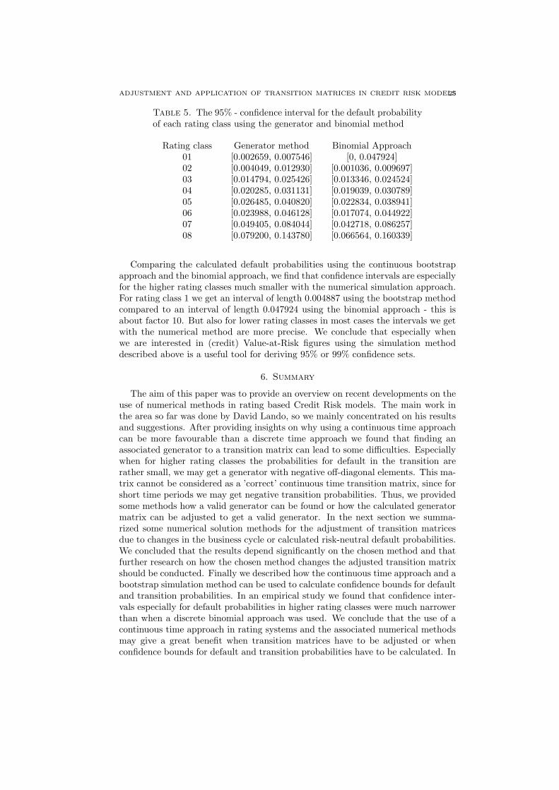
ADJUSTMENT AND APPLICATION OF TRANSITION MATRICES IN CREDIT RISK MODELS25
Table 5. The 95% - confidence interval for the default probabilityof each rating class using the generator and binomial method
Rating class Generator method Binomial Approach01 [0.002659, 0.007546] [0, 0.047924]02 [0.004049, 0.012930] [0.001036, 0.009697]03 [0.014794, 0.025426] [0.013346, 0.024524]04 [0.020285, 0.031131] [0.019039, 0.030789]05 [0.026485, 0.040820] [0.022834, 0.038941]06 [0.023988, 0.046128] [0.017074, 0.044922]07 [0.049405, 0.084044] [0.042718, 0.086257]08 [0.079200, 0.143780] [0.066564, 0.160339]
Comparing the calculated default probabilities using the continuous bootstrapapproach and the binomial approach, we find that confidence intervals are especiallyfor the higher rating classes much smaller with the numerical simulation approach.For rating class 1 we get an interval of length 0.004887 using the bootstrap methodcompared to an interval of length 0.047924 using the binomial approach - this isabout factor 10. But also for lower rating classes in most cases the intervals we getwith the numerical method are more precise. We conclude that especially whenwe are interested in (credit) Value-at-Risk figures using the simulation methoddescribed above is a useful tool for deriving 95% or 99% confidence sets.
6. Summary
The aim of this paper was to provide an overview on recent developments on theuse of numerical methods in rating based Credit Risk models. The main work inthe area so far was done by David Lando, so we mainly concentrated on his resultsand suggestions. After providing insights on why using a continuous time approachcan be more favourable than a discrete time approach we found that finding anassociated generator to a transition matrix can lead to some difficulties. Especiallywhen for higher rating classes the probabilities for default in the transition arerather small, we may get a generator with negative off-diagonal elements. This ma-trix cannot be considered as a ’correct’ continuous time transition matrix, since forshort time periods we may get negative transition probabilities. Thus, we providedsome methods how a valid generator can be found or how the calculated generatormatrix can be adjusted to get a valid generator. In the next section we summa-rized some numerical solution methods for the adjustment of transition matricesdue to changes in the business cycle or calculated risk-neutral default probabilities.We concluded that the results depend significantly on the chosen method and thatfurther research on how the chosen method changes the adjusted transition matrixshould be conducted. Finally we described how the continuous time approach and abootstrap simulation method can be used to calculate confidence bounds for defaultand transition probabilities. In an empirical study we found that confidence inter-vals especially for default probabilities in higher rating classes were much narrowerthan when a discrete binomial approach was used. We conclude that the use of acontinuous time approach in rating systems and the associated numerical methodsmay give a great benefit when transition matrices have to be adjusted or whenconfidence bounds for default and transition probabilities have to be calculated. In

26 STEFAN TRUCK AND EMRAH OZTURKMEN
view of internal-rating based systems and Basel II the benefits of these methodsshould not be neglected.
References
[1] Bomfim, A.N. (2001). Understanding Credit Derivatives and their potential to Synthesize
Riskless Assets. The Federal Reserve Board. Working Paper.
[2] Carty, L., Lieberman D., Fons, J.S. (1995). Corporate Bond Defaults and Default Rates
1970–1994. Special Report. Moody‘s Investors Service.
[3] Carty, L. and Lieberman D. (1996). Corporate Bond Defaults and Default Rates 1938–1995.
Special Report. Moody‘s Investors Service.
[4] Carty, L. (1997). Moody‘s Rating Migration and Credit Quality Correlation, 1920–1996.
Special Comment. Moody‘s Investors Service.
[5] Crosby, P. (1998). Modelling Default Risk. in Credit Derivatives: Trading & Management of
Credit & Default Risk. John Wiley & Sons. Singapore.
[6] Crouhy, M., Galai, D., Mark, R. (2000). A Comparative Analysis of Current Credit Risk
Models. Journal of Banking and Finance (24).[7] Das, S.R. (1998). Credit Derivatives – Instruments. in Credit Derivatives: Trading & Man-
agement of Credit & Default Risk. John Wiley & Sons. Singapore.
[8] Duffie, D. and Singleton, K.J. (1999). Modeling Term Structures of Defaultable Bonds. Re-
view of Financial Studies (12).[9] Efron B. and Tibshirani, R.J (1993). An Introduction to the Bootstrap. Chapman & Hall, New
York. bibitemafoFons, Jerome S. (1994). Using Default Rates to Model the Term Structure
of Credit Risk. Financial Analysts Journal, 25–32.[10] Fons, J.S, Cantor, R., Mahoney C. (2002). Understanding Moody‘s Corporate Bond Ratings
and Rating Process. Special Comment. Moody‘s Investors Service
[11] Gupton, G. (1998). CreditMetrics: Assessing the Marginal Risk Contribution of Credit. inCredit Derivatives: Trading & Management of Credit & Default Risk. John Wiley & Sons.Singapore.
[12] Israel, R.B, Rosenthal, J.S., Wei, J.Z. (2000). Finding Generators for Markov Chains via
Empirical Transition Matrices, with Application to Credit Ratings. Working Paper.
[13] Jarrow, R.A. and Turnbull, S.M. (1995). Pricing Derivatives on Financial Securities Subject
to Credit Risk. Journal of Finance (1).[14] Jarrow, R.A., Lando, D., Turnbull, S.M. (1997). A Markov Model for the Term Structure of
Credit Risk Spreads. Review of Financial Studies (10).[15] Kuchler, U. and Sørensen, M. (1997). Exponential Families of Stochastic Processes. Springer,
New York.[16] Lando, D. (1998). On Cox Processes and Credit Risky Securities. University of Copenhagen.
Working Paper.
[17] Lando, D. (1999). Some Elements of Rating-Based Credit Risk Modeling. University of Cop-nehagen. Working Paper.
[18] Lando, D. and Skødeberg, T. (2000). Analyzing Rating Transitions and Rating Drift with
Continuous Observations. University of Copenhagen. Working Paper.[19] Lando, D. and Christensen, J. (2002). Confidence Sets for Continuous-time Rating Transition
Probabilities. University of Copenhagen. Working Paper.
[20] Madan, D.B. and Unal, H. (1998). Pricing the Risks of Default. Review of Derivatives Re-
search (2).
[21] Merton, R. (1974). On the pricing of corporate debt: The Risk Structure of Interest Rates.
Journal of Finance (29).
[22] Saunders, A. and Allen, L. (2002). Credit Risk Measurement. John Wiley.[23] Schonbucher, P.J. (2000). The Pricing of Credit Risk and Credit Risk Derivatives. University
of Bonn. Working Paper.
[24] Truck, S. and Peppel J. (2003). Credit Risk Models in Practice – A Review. Physica Verlag,
Heidelberg.
[25] Uhrig-Homburg M. (2002). Valuation of Defaultable Claims – A Survey. Schmalenbach Busi-
ness Review (54).[26] Wilson, T.C. (1997). Portfolio Credit Risk I. Risk (10–9).
[27] Wilson, T.C. (1997). Portfolio Credit Risk II. Risk (10–10).