Adjusting to Capital Account Liberalizationkiyotaki/papers/capital account...School of Economics and...
60
Adjusting to Capital Account Liberalization Kosuke Aoki, Gianluca Benigno and Nobuhiro Kiyotaki April, 2006 Preliminary, Appendix to be Completed Abstract We study theoretically how an economy adjusts to liberalization of interna- tional nancial transaction. We consider an economy in which debtors do not repay unless the debts are secured by collateral, and collateralizable assets for international borrowing are more restricted than domestic borrowing. We exam- ine how the adjustment to capital liberalization depends upon the domestic and international collateral constraints. We show that, with an intermediate level of domestic collateral constraint, capital liberalization leads to capital outow, im- provement of TFP, and transitional loss of wage and employment. Government policy can mitigate the loss of workers at the cost of prolonging the transition, but cannot eliminate the loss without halting the transition. London School of Economics, London School of Economics and Bank of England, and London School of Economics and Federal Reserve Bank of New York. 0
Transcript of Adjusting to Capital Account Liberalizationkiyotaki/papers/capital account...School of Economics and...
Adjusting to Capital Account Liberalization
Kosuke Aoki, Gianluca Benigno and Nobuhiro Kiyotaki�
April, 2006Preliminary, Appendix to be Completed
Abstract
We study theoretically how an economy adjusts to liberalization of interna-tional �nancial transaction. We consider an economy in which debtors do notrepay unless the debts are secured by collateral, and collateralizable assets forinternational borrowing are more restricted than domestic borrowing. We exam-ine how the adjustment to capital liberalization depends upon the domestic andinternational collateral constraints. We show that, with an intermediate level ofdomestic collateral constraint, capital liberalization leads to capital out�ow, im-provement of TFP, and transitional loss of wage and employment. Governmentpolicy can mitigate the loss of workers at the cost of prolonging the transition, butcannot eliminate the loss without halting the transition.
�London School of Economics, London School of Economics and Bank of England, and LondonSchool of Economics and Federal Reserve Bank of New York.
0
1 Introduction
"Capital account liberalization, it is fair to say, remains one of the most controversial
and least understood policies of our day". (Eichengreen, 2002)
This paper is a theoretical study into how an economy adjusts to the liberaliza-
tion of international �nancial transaction � capital account liberalization. Although
most economists agree that trade liberalization generally improves e¢ ciency of resource
allocation, they are sharply divided on the costs and bene�ts of capital account lib-
eralization. According to standard microeconomic theory, the international �nancial
transaction is international trade of goods of di¤erent dates (possibly contingent on the
states of nature), and thus capital account liberalization should have similar bene�ts
with trade liberalization. Why do economists disagree? We think that the intertem-
poral exchange of present goods and claims to future goods is fundamentally di¤erent
from intra-temporal exchange of various goods at least in one respect: the intertem-
poral exchange requires commitment that those who made promises in the past keep
their promises to deliver goods (or purchasing power for goods) at the promised date,
while intra-temporal exchange does not require such commitment. If people�s ability to
keep their promises (commitment) is limited, then the equivalence of intertemporal trade
and intra-temporal trade no longer holds, and thus we need to investigate the e¤ects of
capital account liberalization, taking into account the limitation of commitment.
In this paper, we consider an economy in which the debtor (who received present
goods in the past in exchange of a promise of future repayment) does not keep his
promise to repay unless the debt is secured by collateral assets �productive assets he
looses if he defaults. Then, the creditor limits her loan to the debtor so that the
debt repayment does not exceed the value of collateral. Moreover, we consider the
1

amount of collateralizable assets for foreign credits is restricted compared to domestic
credits, because the foreign creditors have more di¢ culty in taking over control and
utilizing the collateral assets in a di¤erent country. Thus, the constraint on international
borrowing is tighter than the domestic borrowing. The extent of collateralizable asset
depends upon both technology and the quality of institution of the economy, which
a¤ects the development of domestic �nancial system. The fraction of future output
from the productive asset usable as collateral for domestic borrowing a¤ects the overall
�nancial depth of the economy. The gap between collateralizable assets for international
borrowing and domestic borrowing �the relative tightness of international borrowing �
a¤ects how much the domestic economy is �nancially integrated into the international
�nancial market. Our aim is to examine how the adjustment of the home economy
to capital account liberalization depends upon the parameter of �nancial depth of the
domestic economy and the relative tightness of the international borrowing constraint.
For this purpose, we construct a dynamic model of small open economy with two
types of in�nitely lived agents: entrepreneurs and workers. At each date, some entrepre-
neurs are productive and other are not. Entrepreneurs hire workers to produce output
in the following period, and they can borrow domestically against only a fraction (do-
mestic collateral factor) of future output. The fraction they can borrow from foreigners
is smaller. The symptom of low domestic collateral factor is that the domestic �nancial
system fails to transfer enough purchasing power from savers (typically unproductive
entrepreneurs) to investing agents (productive entrepreneurs), so that unproductive en-
trepreneurs end up hiring workers. The domestic interest rate remains low �comparable
to the rate of returns on production of the unproductive entrepreneurs , the productive
entrepreneurs are credit constrained, and the total factor productivity (TFP) is low,
2
which leads to low a wage rate.1
The way the economy adjusts to the liberalization of international �nancial transac-
tion depends upon the �nancial depth of the domestic economy and the relative tightness
of the international borrowing constraint. If the domestic �nancial system is poor with
a low �nancial depth, the wage rate is so low before liberalization that even unproduc-
tive entrepreneurs enjoy a higher rate of returns on production than the foreign real
interest rate. After capital liberalization, both productive and unproductive entrepre-
neurs borrow from foreigners, causing capital in�ow, which pushes up the wage rate. If
the international borrowing constraint is tight relative to domestic borrowing constraint
(or if the domestic �nancial depth is lower), then the unproductive entrepreneurs (who
borrow from foreigners) extend domestic loans to the productive entrepreneurs, acting
as �nancial intermediary. Although the workers gain from higher wages, TFP and
accumulation of net wealth of the entrepreneurs stagnate after liberalization.
For the intermediate level of domestic �nancial development, the wage rate is not
very low and the domestic real interest rate under �nancial autarky is below the foreign
interest rate because of �nancial suppression. After capital liberalization, the unproduc-
tive entrepreneurs start lending to foreigners and cutting back their production. With
this capital out�ow, the workers su¤er from loss of wage and employment, and entre-
preneurs gain from a higher rate of return on their net worth. With the intermediate
depth of domestic �nance, capital liberalization serves as a catalyst to reduce ine¢ cient
production, by providing means to absorb the saving which was not productively used
before. The catalyst e¤ect is stronger over time, eliminating the ine¢ cient production
completely, which leads to eventual recovery of the wage rate and employment.
1Kiyotaki and Moore (1997), Kiyotaki (1998), Aghion, Banerjee and Piketty (1999), and Aghion andBanerjee (2005), for examples, investigate these symptoms of the domestic collateral constraint.
3

If domestic �nancial system is more advanced than the rest of the world, the alloca-
tion of production is already e¢ cient, and the large borrowing capacity of the productive
entrepreneurs keeps the domestic interest rate above the foreign rate before liberaliza-
tion. After liberalization, the productive domestic entrepreneurs will attract foreign
fund, causing capital in�ow, increasing the investment on wage bills. Worker gains
from higher wage and employment, and the entrepreneurs gains from cheaper interest
rate. With a superior �nancial institution, the domestic economy can take advantage
of a cheaper fund because of �nancial suppression of the rest of the world.
What emerges from our analysis is that the adjustment of home economy to capital
liberalization depends upon not only the absolute level of development of home �nancial
system, but also on the relative level of development of home institution compared to
the rest of the world.
Because production is ine¢ cient when the domestic �nancial system is poor and
there is painful period of adjustment for workers following capital liberalization for the
economy with intermediate level of �nancial development, a natural step would be to
examine the role of government policy. When people may not keep promises, the analysis
of government policy has new aspects. People may not pay taxes, unless they loose the
collateral asset by not paying taxes. Even if people pay taxes, the tax liability will crowd
out their borrowing capacity, because the debtor may default if the total liabilities to
government and the creditors exceed the value of collateral. Government may default
on its debt too. In the economy with such limited commitment, we show that the
government only reallocates the means of saving (liquidity) between public and private,
instead of creating liquidity (as in Woodford, 2001). For the economy with intermediate
�nancial depth, a small subsidy to production of unproductive entrepreneurs mitigates
the loss of the workers following the capital liberalization at the cost of prolonging the
4

transition to e¢ cient production. But the large subsidy to completely prevent the
temporal loss of workers will halt the transition, ending up hurting both entrepreneurs
and workers in the long run.
There is an extensive literature that examines the relationship between the domestic
�nancial development and capital account liberalization. Aghion, Bacchetta and Baner-
jee (2004) show that the economy with the intermediate level of domestic collateral
factor may become unstable following capital liberalization. Sakuragawa and Hamada
(2001) analyze the danger of capital �ight from South to North following capital liberal-
ization, by constructing an overlapping generations model with costly state veri�cation.
Caballero and Krishnamurthy (2004) emphasize the interaction between domestic and
international �nancial constraints to examine �nancial crisis. Although every entrepre-
neur anticipates the possibility of liquidity shock with some likelihood before the project
yields the return, those who do not experience the shock will earn only meager return on
saving because of limited domestic borrowing capacity and resulting �nancial repression
in the interim period. Thus the entrepreneurs tend to under-save and over-invest in the
�rst place, which makes �nancial crisis likely with small aggregate shock. A recent work
of Caballero, Farhi and Gourinchas (2006) investigate how two economies with di¤er-
ent levels of �nancial depth interact, by using a Blanchard and Yaari type overlapping
generations model. Kim (2001) develops a two country model of adoption of vintages
of technologies, and shows that, following capital liberalization, the country with bet-
ter domestic �nancial system specializes in adopting more recent technology, while the
country with poor �nancial system ends up with adopting older technologies, leading to
a substantial gap in TFP between two. Our distinctive contributions to the literature
would be that we systematically investigate the implications of limited commitment of
both private and government agents against both domestic and foreign creditors, for the
5

entire adjustment process of the economy to capital account liberalization.
2 Model
We consider a small open economy with one homogeneous goods and two types of con-
tinua of agents: entrepreneurs and workers. Both of them live forever. Entrepreneurs
hire workers to produce goods. Workers do not have production technology, simply
supplying homogeneous labour in order to consume.
The preference of the entrepreneur is described by the expected discounted utility
Et
" 1Xs=t
�s�t log cs
#; (1)
where cs is the consumption at date s; and � 2 (0; 1) is the subjective discount factor,
and Et is the expectations conditional on information at date t.
The entrepreneurs have a constant returns to scale production technology
yt+1 = atlt; (2)
where yt+1 is output of goods at date t + 1, lt is the labour input at date t, and at is a
productivity parameter, which is known at date t. At each date some entrepreneurs are
productive (at = �); and others are unproductive (at = 2 (0; �)). Each entrepreneur
shifts stochastically between productive and unproductive states following a Markov
process. Speci�cally, if an entrepreneur is productive in this period he/she may become
unproductive in the next period with probability �: Also, any unproductive entrepreneur
in this period may become productive in the next period with probability n�: The shifts
6

of the productivity are exogenous and independent across entrepreneurs and over time.
This transition matrix implies that the fraction of productive entrepreneurs is stationary
over time and equal to n=(1 + n), given that the economy starts with such population
distribution. We assume that the probability of the productivity shifts is not too large:
� + n� < 1: (3)
This assumption is equivalent to the condition that the productivity of each agent is
positively correlated between present and the next periods.
We assume that the production technology is speci�c to the entrepreneur, and that
only the entrepreneur who started the production has the necessary skill to obtain full
amount described by the production function. We also assume that the entrepreneur
cannot precommit to work, always having freedom to withdraw its labour. (The en-
trepreneur�s human capital is inalienable, following Hart and Moore (1994)). Besides
this entrepreneur, a lead creditor who has been monitoring the production throughout
has a speci�c skill to obtain � (< 1) fraction of full amount of output, if she takes over
the entrepreneur�s production. Although production is divisible, we assume that there
is only one lead creditor for each segment of production, and that only a home resident
can become a lead creditor. All the other (non-lead) outside creditors, home or foreign,
can obtain only �� fraction of full output, where � 2 [0; 1). If the entrepreneur who
borrows to produce threatens to withdraw its labour immediately before output realizes
in order to negotiate with the creditors, it is e¢ cient for the entrepreneur to bribe the
creditors into letting him to continue production. Assuming that the outside creditors
(including foreign lenders) are weak in the bargaining against the entrepreneur and the
lead creditor, the repayment to the outside creditors is negotiated down to �� fraction of
7
full output2. Knowing this possibility in advance, the foreign lenders restrict their loan
of this period so that the repayment (b�t+1) does not to exceeds �� fraction of output in
the next period:
b�t+1 � ��yt+1: (4)
Also, assuming that the creditors as a whole are weak against the entrepreneur in the
bargaining, the domestic lead creditor restricts her loan (bt+1) so that the total sum of
loans does not exceed � fraction of output,:
bt+1 + b�t+1 � �yt+1: (5)
We take both � and � as exogenous parameters to represent the degrees of devel-
opment of the country�s �nancial institution. We consider the size of � as a domestic
collateral factor, representing the overall �nancial depth of the home economy. The gap
between �� and � re�ects the di¤erence between the outside creditors and the lead cred-
itor in their skills of production and bargaining, (being in�uenced by legal protection of
the outside creditors3), which explains why borrowing constraint from the foreigners is
tighter than the borrowing constraint from the domestic lead creditor. We assume that
the collateralized return from unit labour input of productive entrepreneurs is smaller
than the return of unproductive entrepreneurs:
�� < : (6)
2Diamond and Rajan (2001) called the lead creditor relationship banker. Unlike Diamond and Rajan,however, we consider an economy in which the lead creditor cannot precommit to bargain sequentiallywith one outsider creditor after another in order to give up her bargaining power.
3See La Porta, Shleifer, Lopez-de-Silanes and Vishny (1998, 2002).
8
Under this assumption, the productive entrepreneurs cannot borrow unlimited amount
when the interest rate is at least as high as the rate of return on production of the
unproductive entrepreneurs.
The �ow-of-funds constraint of the entrepreneur is given by
ct + wtlt = yt � bt � b�t +bt+1rt
+b�t+1r�; (7)
where wt is the real wage rate, rt is the domestic real gross interest rate, and r� is the
foreign real gross interest rate. The left hand side (LHS) of the �ow-of-fund constraint
is expenditure; consumption (ct) and investment �wage bill (wtlt) due to the time lag
between labour input and output in production function. The right-hand-side (RHS) is
�nancing; the internal �nance from the net worth �output minus the debt repayment
to domestic and foreign creditors �, and the external �nance of the borrowings from
home and foreign creditors. Throughout the analysis, we assume the home economy is
small relative to the rest of the world, the real interest rate of the rest of the world is
constant over time, and that there is no limitation on domestic lending to foreigners at
this interest rate. We also assume the foreign interest rate is strictly less than the time
preference rate:
r� < 1=�: (8)
The entrepreneur chooses consumption, labour input, output and domestic and foreign
borrowing�ct; lt; yt+1; bt+1; b
�t+1
�to maximize the expected discounted utility (1) subject
to the constraints of technology (2), the �ow-of-funds (7), the borrowing from foreign
and home creditors (4) and (5).
Next, we turn to workers. Unlike entrepreneurs, the workers do not have production
technology, nor any collateralizable asset in order to borrow either domestically or in-
9

ternationally. They choose consumption ct, labour supply lt, and domestic and foreign
net borrowings (bt+1 and b�t+1) to maximize the expected discounted utility,
Et
" 1Xs=t
�s�tu (cs � v(lt))#; (9)
subject to the �ow of funds constraint
ct = wtlt � bt � b�t +bt+1rt
+b�t+1r�; (10)
and the borrowing constraints
bt+1 � 0; b�t+1 � 0: (11)
We assume decreasing marginal net utility of consumption, u0(c� v) > 0; u"(c� v) < 0;
and increasing marginal disutility of labour, v(0) = 0; v0(l) > 0; v"(l) > 0: The choice of
labour supply implies wt = v0(lt); or
lst = Ls(wt); where Ls(w) = v0�1(l): (12)
Thus dLs=dwt > 0: We normalize the population size of workers to be unity.
Let us denote aggregate consumption of productive entrepreneurs, unproductive en-
trepreneurs, and workers as Ct; C 0t; and Cwt : (Similarly let Bt; B
0t; and B
wt be aggregate
quantities of the other quantity bt of productive entrepreneurs, unproductive entrepre-
neur, and workers, etc.). The market clearing condition for labour, goods, and domestic
credit are written as
Lt + L0t = L
s(wt); (13)
10
Ct + C0t + C
wt = Yt + Y
0t +
B�t+1r�
�B�t ; (14)
Bt+1 +B0t+1 +B
wt+1 = 0: (15)
In the RHS of equation (14), B�t is de�ned as the aggregate net debt of all the home
entrepreneurs and workers against foreigners matured at date t, and thus the last two
terms are the net supply of goods by the foreigners to domestic agents. In equation
(15), the debt of domestic agents to the other domestic agents should be net out in the
aggregate, even though the total debts of the domestic agents need not because of the
international borrowing and lending. (Remember that the domestic credit market may
be segmented from the international credit market, because the home agents face the
international borrowing constraint).
The competitive equilibrium is de�ned as a set of prices (rt; wt) and quantities
(yt; lt; ct; bt+1; b�t+1; Yt; Y
0t ; Lt:L
0t; Ct; C
0t; C
wt ; Bt+1; B
0t+1; B
wt+1; B
�t+1); which is consistent of
the choice of all the individual entrepreneurs and workers as well as the clearing con-
ditions of market for labour, goods and domestic credit. Because there is no shocks
except for the idiosyncratic shock to the productivity of each entrepreneur, the agents
have perfect foresight of future prices and aggregate quantities in the equilibrium. By
Walras�Law, only two out of three market clearing conditions are independent.
Now, let us derive general property of the competitive equilibrium. In our small open
economy, although home agents face the constraint on their borrowing from foreigners,
there is no constraint on their lending to foreigners: Thus, in equilibrium, we learn that
the domestic interest rate is at least as high as the foreign interest rate:
rt � r�: (16)
11
(If the domestic interest rate were strictly lower than the foreign interest rate, there
would be no domestic agent who provides domestic credit and there would be many
producers who seek domestic credit, which contradicts the market equilibrium).
The entrepreneur has a few choices of accumulating net worth from this period to
the next period subject to the �ow-of-funds constraint (7). Let Rt(at) be the maximum
rate of returns on the net worth from date t to date t+1 for the entrepreneur with labour
productivity at: Then, it is the maximum of all the options as:
Rt(at) =Max
�rt;
atwt;
at(1� ��)wt � (at��=r�)
;at(1� �)
wt � (at��=r�)� [at(1� �)�=rt]
�: (17)
The �rst term in the bracket of RHS is the rate of return on domestic loan; which is
at least as high as the return on making loan to the foreigners by (16): The second
term is the rate of returns on production without borrowing, subject to the constraint
of production technology (2): The third term is the rate of return on production with
borrowing from foreigners by putting �� fraction of output as collateral ((4) holds with
equality and lt > 0 in the �ow-of-funds constraint). By borrowing from foreigners
secured by �� fraction of output, the entrepreneur can �nance at��=r� amount of unit
labour cost externally. Thus the denominator is the required net worth (downpayment)
for the unit labour input, and the numerator is the output after repaying the debt.
The �nal term is the rate of returns on production with maximum borrowing from
both foreigners and the domestic lead creditor. (Both (4) and (5) hold equality and
lt > 0 in the �ow-of-funds constraint). The denominator is downpayment for hiring unit
labour, when the entrepreneur �nances at��=r� of unit labour cost from borrowing from
foreigners, and �nances at(1� �)�=rt by borrowing additionally from the domestic lead
creditor at interest rate rt: (Note that the entrepreneur prefers to borrow maximum
12
�rst from foreigners at a lower interest rate4).
Given this optimal choice of accumulating net worth, the �ow-of-funds constraint (7)
can be written as
mt+1 = Rt(at)(mt � ct); (18)
where mt (= yt � bt � b�t ) is net worth of the entrepreneur at date t. The entrepreneur
chooses consumption and saving in order to maximize the expected discounted utility
subject to the �ow-of-fund constraint. The �rst order condition is given by the Euler
equation:1
ct= �Rt(at)Et
�1
ct+1
�:
Together with the �ow-of-funds constraint, we have the explicit consumption function
as
ct = (1� �)mt = (1� �)(yt � bt � b�t ): (19)
In the expression of maximum rate of returns on net worth (17); each of the last three
rates of returns on production are strictly higher for the productive entrepreneur than
the unproductive entrepreneur, while the rate of return on domestic loan is the same
for both. Thus, the unproductive entrepreneur has comparative advantage in providing
loan, while the productive entrepreneurs have comparative advantage in production with
maximum borrowing. Later, we will show that the workers will not lend nor borrow
in the equilibrium, so that the domestic debts of the productive and the unproductive
entrepreneurs are net out in the domestic credit market. Thus we learn that unproduc-
tive entrepreneurs lend to productive entrepreneurs in the domestic credit market, and
4The preference is strict if r� < rt: If r� = rt; then entrepreneur is indi¤erent, and any combinationof doemstic and foreign borrowing yields the same return as long as the sum of borrowing is at themaxmimum.
13

that
Rt( ) = rt �Max�
wt; (1� ��)
wt � ( ��=r�)
�; (20)
0 = l0
t
�rt �Max
�
wt; (1� ��)
wt � ( ��=r�)
��:
The unproductive entrepreneurs produce if and only if the rate of return on produc-
tion is equal to the domestic interest rate. Otherwise, the unproductive entrepreneurs
specialize in providing loan.
We also learn that the productive entrepreneur always borrows to produce, and that
their domestic and international borrowing constraints are binding if the rate of return
on production with maximum leverage exceeds the domestic interest rate:
Rt(�) =�(1� �)
wt � (���=r�)� [�(1� �)�=rt]� rt;
lt ��mt
wt � (���=r�)� [�(1� �)�=rt]; and the equality holds if Rt(�) > rt: (21)
We derive the expression of upper bound of employment of the productive entrepre-
neur from the two borrowing constraints with equality, the �ow-of-funds constraint and
consumption function, (4) (5) (7); and (19): Let Zt be aggregate net worth of all the
entrepreneurs
Zt = Yt + Y0t �Bt �B0t �B�t ;
and let st be the share of net worth of all the productive entrepreneurs, so that stZt is
the aggregate net worth of the productive entrepreneurs. Because the labour demand
function of the productive entrepreneur (21) is linear and common to all the productive
entrepreneurs, we can derive the aggregate employment of the productive entrepreneurs
14

as
Lt ��stZt
wt � (���=r�)� [�(1� �)�=rt]; and the equality holds if Rt(�) > rt: (22)
Concerning the workers, they will decumulate their asset until they consume all, if
the domestic real interest rate is strictly less than the time preference rate:
rt < 1=�: (23)
We will later verify this inequality holds in equilibrium. When workers consume all
the asset, ideally they would like to borrow, but they cannot borrow because they do
not have collateral. Thus, after the initial transition, the workers�asset stays zero with
the borrowing constraint (11) binding, and the aggregate consumption of the workers is
equal to the aggregate wages5:
Bwt = 0; and Cwt = wtL
s(wt): (24)
The workers do not save, not because the workers are impatient relative to the entre-
preneurs, but because the real interest rate is lower than the time preference rate in
equilibrium. The entrepreneurs nonetheless save because their rate of return on net
worth exceeds the time preference rate when they are productive.
From the behavior of the workers, the domestic credit market equilibrium becomes
Bt + B0t = 0. Together with the consumption function of the entrepreneurs (19) ; the
5If the workers expect sharp decline of wage in furure, then they may save despite of the interestrate being lower than the time preference rate. We will later show that there is no such sharp andcontinual decline in wages in the equilibrium.
15
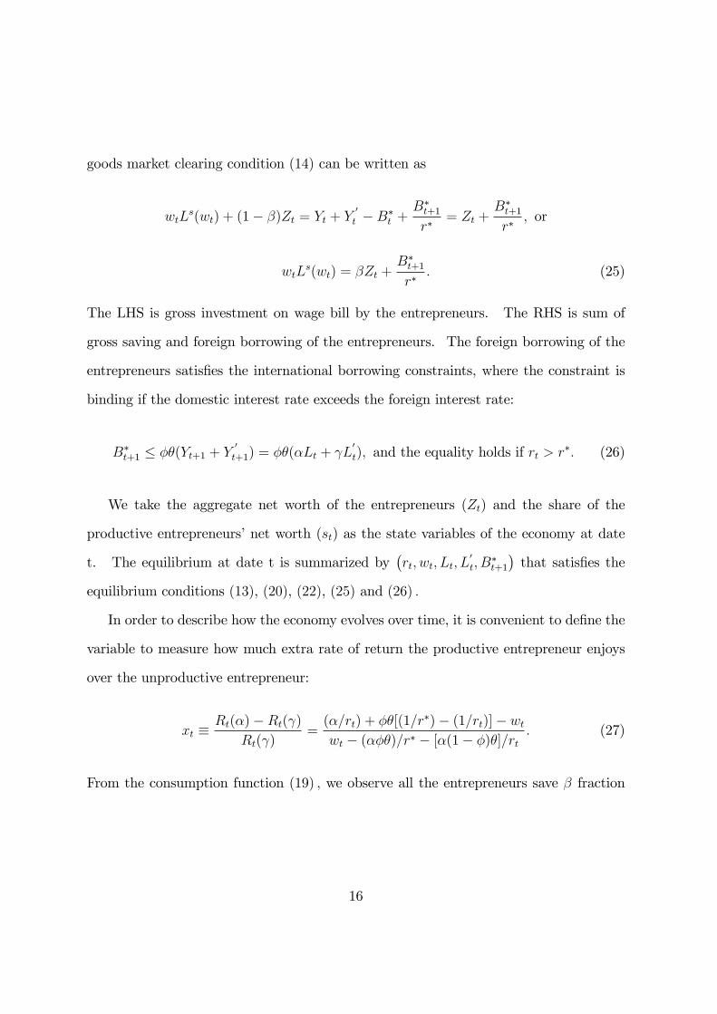
goods market clearing condition (14) can be written as
wtLs(wt) + (1� �)Zt = Yt + Y
0
t �B�t +B�t+1r�
= Zt +B�t+1r�
; or
wtLs(wt) = �Zt +
B�t+1r�
: (25)
The LHS is gross investment on wage bill by the entrepreneurs. The RHS is sum of
gross saving and foreign borrowing of the entrepreneurs. The foreign borrowing of the
entrepreneurs satis�es the international borrowing constraints, where the constraint is
binding if the domestic interest rate exceeds the foreign interest rate:
B�t+1 � ��(Yt+1 + Y0
t+1) = ��(�Lt + L0
t); and the equality holds if rt > r�: (26)
We take the aggregate net worth of the entrepreneurs (Zt) and the share of the
productive entrepreneurs�net worth (st) as the state variables of the economy at date
t. The equilibrium at date t is summarized by�rt; wt; Lt; L
0t; B
�t+1
�that satis�es the
equilibrium conditions (13), (20), (22), (25) and (26) :
In order to describe how the economy evolves over time, it is convenient to de�ne the
variable to measure how much extra rate of return the productive entrepreneur enjoys
over the unproductive entrepreneur:
xt �Rt(�)�Rt( )
Rt( )=(�=rt) + ��[(1=r
�)� (1=rt)]� wtwt � (���)=r� � [�(1� �)�]=rt
: (27)
From the consumption function (19) ; we observe all the entrepreneurs save � fraction
16

of their net worth. Then, the aggregate wealth in the next period would be:
Zt+1 = (1 + xt)rt�stZt + rt�(1� st)Zt (28)
= (1 + stxt)rt�Zt:
Here, the aggregate saving of productive entrepreneurs (�stZt) earns the rate of returns
Rt (�) = (1+xt)rt; while the aggregate saving of the unproductive entrepreneurs (�(1�
st)Zt) only earns the rate of return Rt ( ) = rt: We can also derive the law of motion
of the share of productive entrepreneurs�net worth as:
st+1 =(1� �)(1 + xt)rt�stZt + n�rt�(1� st)Zt
(1 + stxt)rt�Zt(29)
=(1� �)st(1 + xt) + n�(1� st)
1 + stxt:
The denominator of RHS of the �rst equation is the aggregate net worth in the next pe-
riod. The numerator is the aggregate net worth of productive agents in the next period,
which is the sum of the net worth of those who continue to be productive, (1 � �)(1 +
xt)rt�stZt; and those who shift from unproductive to be productive, n�rt�(1 � st)Zt.
The dynamic evolution of the economy is characterized by the recursive equilibrium:�Zt+1; st+1; xt; rt; wt; Lt; L
0t; B
�t+1
�that satis�es (13), (20), (22), (25), (26), (27), (28) and
(29); as functions of the state variables (st; Zt):
3 Steady State Autarky Equilibrium
Before looking into how the economy adjusts to the capital liberalization, we �rst analyze
the steady state equilibrium of the economy with no �nancial transaction with foreigners.
17

Here, the home agents are not allowed to borrow nor lend, i.e., � = B�t = 0: Because
our economy has only one goods and labour is not tradeable, once there is no trade of
�nancial assets, there would be no trade of goods in equilibrium: the economy becomes
autarky. In the steady state, all the endogenous variables stay constant. Let us
de�ne X = sx; the product of the share of net worth and the extra rate of returns of
the productive agents �the importance of extra returns of the productive entrepreneurs.
Then, the equilibrium conditions (13), (20), (22),(25), (27), (28) and (29) can be written
as
L+ L0 = Ls(w); (30)
r �
w; and L0(r �
w) = 0; (31)
L � X
(�=r)� w�Z; and the equality holds if�
r> r: (32)
wLs(w) = �Z; (33)
x =(�=r)� ww � (��=r) ; (34)
1 = �(1 +X)r; (35)
F (X; x) = X2 + [�(1 + n)� (1� �)x]X � n�x = 0; and X � 0: (36)
In the steady state equilibrium of the autarky economy, these seven equilibrium condi-
tions determine (r; w; x;X; L; L0; Z) endogenously. Then, we have the following propo-
sition (See Figure 1. Proofs of all the Propositions are in Appendix):
Proposition 1 The steady state equilibrium of the autarky economy depends upon the
�nancial depth of the economy � as:
(i) If � < � � ��� +(1+n)�
; the unproductive entrepreneurs produce in equilibrium,
18
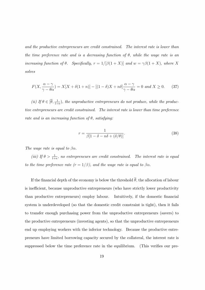
and the productive entrepreneurs are credit constrained. The interest rate is lower than
the time preference rate and is a decreasing function of �; while the wage rate is an
increasing function of �. Speci�cally, r = 1=[�(1 +X)] and w = �(1 +X); where X
solves
F (X;�� � ��) = X[X + �(1 + n)]� [(1� �)X + n�]
�� � �� = 0 and X � 0: (37)
(ii) If � 2 [�; 11+n); the unproductive entrepreneurs do not produce, while the produc-
tive entrepreneurs are credit constrained. The interest rate is lower than time preference
rate and is an increasing function of �, satisfying:
r =1
�[1� � � n� + (�=�)] : (38)
The wage rate is equal to ��:
(iii) If � > 11+n; no entrepreneurs are credit constrained. The interest rate is equal
to the time preference rate (r = 1=�), and the wage rate is equal to ��:
If the �nancial depth of the economy is below the threshold �; the allocation of labour
is ine¢ cient, because unproductive entrepreneurs (who have strictly lower productivity
than productive entrepreneurs) employ labour. Intuitively, if the domestic �nancial
system is underdeveloped (so that the domestic credit constraint is tight), then it fails
to transfer enough purchasing power from the unproductive entrepreneurs (savers) to
the productive entrepreneurs (investing agents), so that the unproductive entrepreneurs
end up employing workers with the inferior technology. Because the productive entre-
preneurs have limited borrowing capacity secured by the collateral, the interest rate is
suppressed below the time preference rate in the equilibrium. (This veri�es our pre-
19

vious conjecture (23)): Since production allocation is ine¢ cient, the aggregate wealth
and the wage rate are remained to be low in the steady state. The threshold level � of
domestic collateral factor to induce the productive ine¢ ciency is an increasing function
of the transition probability from the productive to unproductive state �; because the
higher the transition probability is; the lower is the share of net worth of the productive
entrepreneurs, and the smaller is the aggregate borrowing capacity of the productive
entrepreneurs relative to the aggregate saving.6.
In the second type of equilibrium, � is at least as large as � but smaller that the
share of population of the unproductive entrepreneurs, 1=(1 + n). Here, the domestic
�nancial system is developed enough to transfer necessary purchasing power to produc-
tive entrepreneurs to achieve the e¢ ciency in production. (The e¢ ciency in production
means aggregate output is at the maximum for a given total employment. It does not
mean the allocation is the �rst best, because the credit constraint is binding). Then,
the larger the borrowing capacity of the productive entrepreneurs is, the larger is the
demand for domestic credit relative to the supply, and the higher is the equilibrium
interest rate in the domestic credit market. This explains why the interest rate is an
increasing function of �.
If the domestic �nancial system is very well developed � > 11+n
in the third type
equilibrium, both the productive and unproductive entrepreneurs enjoy the same rate of
return on saving, behaving similarly, and thus the entrepreneurs as a whole behave like
the representative entrepreneur.7 The economy achieves the �rst best allocation with
6A higher � implies the economy is more likely to be ine¢ cient in production for the same �nancialdepth. The threshold � is also a decreasing function of the productivity gap between productive andunproductive entrepreneurs (�� )= , because the larger the gap is, the larger is the share of net worthof the productive entrepreneurs, and the larger is their borrowing capacity relative to aggregate saving.
7For � < 1=(1 + n); Proposition 1 veri�es our conjecture (23). Because (23) no longer holds for� � 1=(1 + n), workers may not be credit constrained. Also, we must use (22) instead of (32) in order
20
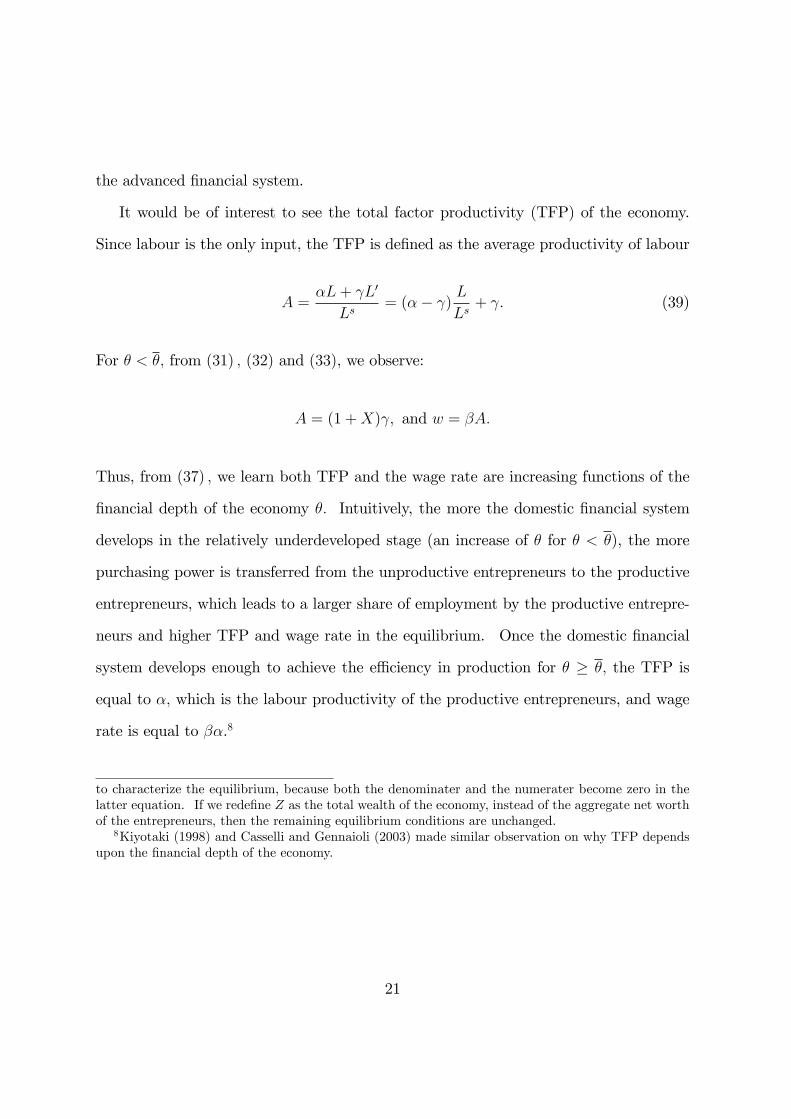
the advanced �nancial system.
It would be of interest to see the total factor productivity (TFP) of the economy.
Since labour is the only input, the TFP is de�ned as the average productivity of labour
A =�L+ L0
Ls= (�� ) L
Ls+ : (39)
For � < �; from (31) ; (32) and (33), we observe:
A = (1 +X) ; and w = �A:
Thus, from (37) ; we learn both TFP and the wage rate are increasing functions of the
�nancial depth of the economy �: Intuitively, the more the domestic �nancial system
develops in the relatively underdeveloped stage (an increase of � for � < �), the more
purchasing power is transferred from the unproductive entrepreneurs to the productive
entrepreneurs, which leads to a larger share of employment by the productive entrepre-
neurs and higher TFP and wage rate in the equilibrium. Once the domestic �nancial
system develops enough to achieve the e¢ ciency in production for � � �; the TFP is
equal to �; which is the labour productivity of the productive entrepreneurs, and wage
rate is equal to ��.8
to characterize the equilibrium, because both the denominater and the numerater become zero in thelatter equation. If we rede�ne Z as the total wealth of the economy, instead of the aggregate net worthof the entrepreneurs, then the remaining equilibrium conditions are unchanged.
8Kiyotaki (1998) and Casselli and Gennaioli (2003) made similar observation on why TFP dependsupon the �nancial depth of the economy.
21

4 Adjusting to Capital Liberalization
We now study how the economy is going to adjusts to the liberalization of �nancial
transactions with foreigners, starting from the steady state autarky equilibrium. We
are going to focus on the situation in which the productive entrepreneurs are credit
constrained, (i.e., equation (22) holds with equality). Later, we will derive the condition
for this to be true, (and will discuss how our results are extended for the case in which
the productive entrepreneurs are not credit constrained). Combining (13) with (20) and
(22) ; we can summarize the labour market equilibrium condition as9:
Ls(wt) ��stZt
wt � (���=r�)� [�(1� �)�=rt]; (40)
rt � (1� ��)
wt � ( ��=r�); (41)
�Ls(wt)�
�stZtwt � (���=r�)� [�(1� �)�=rt]
��rt �
(1� ��)wt � ( ��=r�)
�= 0: (42)
For given state variables (st; Zt) ; the interest rate rt that satis�es (40) with equality is
a decreasing function of the wage rate wt; so is the interest rate that satis�es (41) with
equality. Because we know
�Ls(wt)�
�stZtwt � (���=r�)� [�(1� �)�=rt]
�rt=
(1���)wt�( ��=r�)
is an increasing function of wt, when (41) holds with equality, the inequality (40) is
satis�ed for wt � w� and is violated for wt < w� for some w�: Thus, the labour market
equilibrium locus of (wt; rt) is described by ABC in Figure 2.
9From rt � r�, we know the second term in the bracket of RHS of (20) is at least as large as the�rst term.
22

From equations (25) (26) and (22) ; the goods market equilibrium condition is sum-
marized by inequality (16) and:
�Zt
�1 +
(�� )(��=r�)stwt � (���=r�)� [�(1� �)�=rt]
���wt �
��
r�
�Ls (wt) ; (43)
��Zt
�1 +
(�� )(��=r�)stwt � (���=r�)� [�(1� �)�=rt]
���wt �
��
r�
�Ls (wt)
�(rt � r�) = 0:
(44)
The goods market equilibrium is described by the DEF in Figure 3:
Given the state variables (st; Zt) ; the equilibrium of date t is described by (wt; rt)
that clears both labour and goods markets, i.e., the intersection of curves ABC of Figure
2 and DEF of Figure 3. When (40) holds with equality; the inequality (43) can be
rewritten as
�Zt � Ls(wt)�wt �
���
r�
�:
Thus, if (40) holds with equality; the inequality (43) is satis�ed for wt � w��; and it
is violated if wt > w�� for some w��: Then, the locus of (wt; rt) that satis�es (43)
with equality is steeper than the locus that satis�es (40) with equality, which is in turn
steeper than the locus that satis�es (41) with equality. Therefore, there exists a unique
intersection of the labour market equilibrium locus and the goods market equilibrium
locus, and there are four possible types of equilibrium (See Figure 4).
Proposition 2 For a given state variables (st; Zt) ; there exists a unique date t equilib-
rium of one of the four types:
(Type A : L0t > 0 and rt > r�) (41) and (43) hold with equality, and (40) with strict
inequality;
(Type B : L0t > 0 and rt = r�) (41) holds with equality, (40) with strict inequality,
23

and (43) with inequality;
(Type C : L0t = 0 and rt = r�) (40) holds with equality, and (41) (43) with inequality;
(Type D : L0t = 0 and rt > r�) (40) (43) hold with equality, and (41) with strict in-
equality.
In equilibrium of Type A and Type B; the production allocation is ine¢ cient as the
unproductive entrepreneurs employ labour. In contrast, the production is e¢ cient in
equilibrium of Type C and Type D: In equilibrium of Type B and Type C; the domestic
credit market is integrated into the international credit market, so that the domestic and
foreign interest rates are equal. In equilibrium of Type A and Type D; on the other
hand, the domestic interest rate exceeds the foreign interest rate, so that the domestic
credit market is segmented from the international credit market.
Using Propositions 1 and 2, we can describe the economy immediately after the
capital liberalization. Let rA (�) ; wA(�); sA(�) and ZA(�) be the domestic interest
rate, wage rate, share of net worth of the productive entrepreneurs and the aggregate
net worth of the entrepreneurs in the steady state equilibrium of autarky economy with
�nancial depth �: From Proposition 1, we know rA (�) is a decreasing function of � for
� < �, and is an increasing function of � for � � �. Let us assume that
rA(�) =
��< r�: (45)
The inequality implies that the foreign interest rate is higher than the minimum value of
the domestic interest rate in the steady state autarky equilibrium for all possible �nancial
depth of the home economy. (If the foreign economy has the same environment as the
home economy except for the �nancial depth, then this assumption holds except for an
exceptional case that foreign �nancial depth is exactly equal to �). Let us de�ne two
24
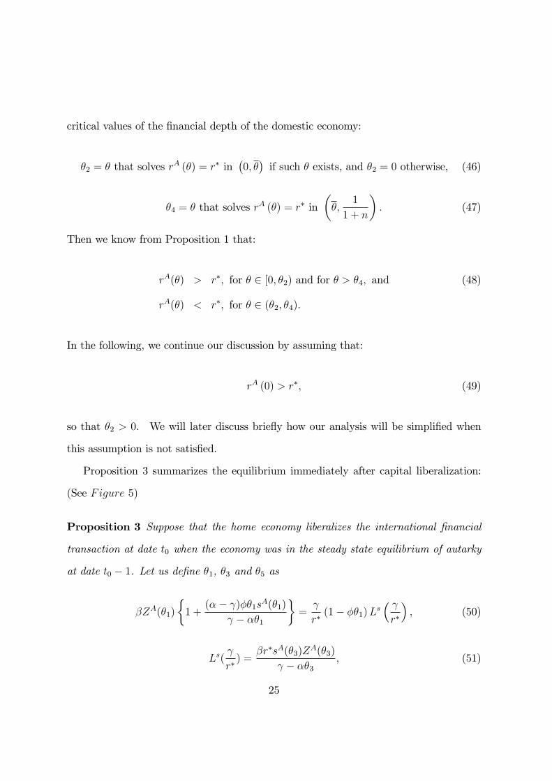
critical values of the �nancial depth of the domestic economy:
�2 = � that solves rA (�) = r� in�0; ��if such � exists, and �2 = 0 otherwise, (46)
�4 = � that solves rA (�) = r� in��;
1
1 + n
�: (47)
Then we know from Proposition 1 that:
rA(�) > r�; for � 2 [0; �2) and for � > �4; and (48)
rA(�) < r�; for � 2 (�2; �4):
In the following, we continue our discussion by assuming that:
rA (0) > r�; (49)
so that �2 > 0. We will later discuss brie�y how our analysis will be simpli�ed when
this assumption is not satis�ed.
Proposition 3 summarizes the equilibrium immediately after capital liberalization:
(See Figure 5)
Proposition 3 Suppose that the home economy liberalizes the international �nancial
transaction at date t0 when the economy was in the steady state equilibrium of autarky
at date t0 � 1. Let us de�ne �1, �3 and �5 as
�ZA(�1)
�1 +
(�� )��1sA(�1) � ��1
�=
r�(1� ��1)Ls
� r�
�; (50)
Ls(
r�) =
�r�sA(�3)ZA(�3)
� ��3; (51)
25
�5 = Min(1� n�r�
1 + n
Ls(��)
Ls(�=r�); �05); where (52)�
w(�05)� ���05r�
�Ls(w(�05) = �ZA(�05), and w(�) solves
�w(�)� ��
r�
�Ls(w (�)) = �sA(�)ZA(�):
We learn
0 < �1 < �2 < �3 < � < �4 < �5;
and that the equilibrium at date t0 is:
(Type A: L0t0 > 0; rt0 > r�), if � 2 [0; �1);
(Type B: L0t0 > 0; rt0 = r�), if � 2 [�1; �3);
(Type C: L0t0 = 0; rt0 = r�), if � 2 [�3; �5];
(Type D: L0t0 = 0; rt0 > r�), if � 2 (�5; 1):
Notice that the minimum level of the �nancial depth of the home economy to achieve
the productive e¢ ciency falls from � to �3 immediately after capital liberalization. Thus,
the economy is more likely to achieve the e¢ ciency in production after capital liberal-
ization than the autarky economy for the same �nancial depth. Intuitively, the interna-
tional capital market provides additional means to absorb the saving of the unproductive
entrepreneurs and to reduce ine¢ cient production, especially when the domestic �nan-
cial system is underdeveloped relatively to the rest of the world but it is not extremely
underdeveloped. Also, we observe that capital liberalization does not necessarily leads
to the complete �nancial integration of the home economy with the rest of the world im-
mediately after the liberalization. If the �nancial depth of the economy is very di¤erent
from the rest of the world, either extremely low � < �1 or extremely high � > �5; the do-
mestic interest rate stays higher than the foreign interest rate because the international
26

borrowing constraint is binding.10
How does the new steady state after capital liberalization depends upon the �nancial
depth of the domestic economy? From the generic equilibrium conditions, (13), (20),
(22),(25), (26) (27), (28) and (29) ; we learn the steady state equilibrium of the open
economy is characterized by (r; w; x;X; L; L0; Z) that satis�es the conditions (30), (35),
(36) and
r � (1� ��)w � ( ��=r�) ; and
�r � (1� ��)
w � ( ��=r�)
�L0 = 0; (53)
L =�XZ
(�=r)� w + ���[(1=r�)� (1=r)] ; (54)
�Z +��
r�[ Ls(w) + (�� )L] � wLs(w); and (55)
(r � r�)��Z +
��
r�[ Ls(w) + (�� )L]� wLs(w)
�= 0;
x =(�=r)� w + ��� [(1=r�)� (1=r)]w � (��=r)� ��� [(1=r�)� (1=r)] : (56)
From these conditions, we have the following proposition (See Figure 6):
Proposition 4 Let r(�), w(�) and Z(�) be the domestic interest rate, the wage rate and
the aggregate net worth of the entrepreneurs in the steady state equilibrium of the open
economy with �nancial depth of �. The equilibrium depends upon the �nancial depth of
the home economy as:
(i) If � < �2; the unproductive entrepreneurs produce. r� < r(�) < rA(�), w (�) >
wA(�), r0(�) < 0 and w0(�) > 0:
(ii) If � 2 [�2;e�]; where e� � �+��[n�+(1=�r�)�1](1+n)�+(1=�r�)�1 2 (�4; 1); the unproductive entrepreneurs
10For the economy with � > 1� n�r�
1+nLs(��)Ls(�=r�) ; the productive entreprenerus are not credit constrained.
However, the equilibrium is still Type D.
27

do not produce, r(�) = r� and w0(�) > 0:
(iii) If � > e�; the unproductive entrepreneurs do not produce, r(�) > r�; w(�) >
wA(�); r0(�) � 0 and w0(�) > 0:
(iv) Z (�) is an increasing function of �, if labour supply is relatively elastic:
w
LsLs0(w) >
(n�=X�) + 1 + [(1 + n)� +X�](� � �2)n� +X� � [(1 + n)� +X�](� � �2)
; where X� � 1
�r� 1 > 0: (57)
Note that the unproductive entrepreneurs do not produce if the �nancial depth is at
least as high as �2: Thus the economy is more likely to achieve e¢ ciency in production for
the same �nancial depth in the steady state than the equilibrium immediately after the
liberalization, (because �2 < �3 of Proposition 3). Also, we see that Type B equilibrium
with ine¢ cient production and complete �nancial integration no longer exists in the
steady state. Intuitively, the international capital market has a stronger catalyst e¤ect
of eliminating the ine¢ ciency in production in the long run than the short run, so that
the ine¢ ciency of production remains in the long run only if the domestic �nancial
market is not perfectly integrated with the international �nancial market.11
From Proposition 4, we learn the wage rate is an increasing function of the �nancial
depth of the economy �, so is the total employment of the economy (which is equal
to labour supply). The aggregate net worth of the entrepreneurs depends upon both
aggregate output and income distribution between entrepreneurs, workers and foreigners.
The more developed the domestic �nancial system is, the larger is the aggregate output,
and the less favorable is the income distribution of the entrepreneurs after achieving
the e¢ ciency in production. Proposition 4(iv) says the aggregate net worth of the
entrepreneurs is an increasing function of the �nancial depth if labour supply is relatively
11If � is close enough to 1, then the productive entrepreneurs are not credit constrained, but thesteady state equilibrium is still characterized by (iii).
28

elastic. Although the threshold elasticity of labour supply is higher than 1, we are
focusing on relatively underdeveloped economy which tends to have elastic labour supply,
and thus we are going to continue the analysis under the assumption of (57) :12
In order to understand the transition from the economy immediately after liberal-
ization (in Proposition 3) to the new steady state (in Proposition 4), we examine the
dynamics of the aggregate net worth of the entrepreneurs (Zt) and the share of net worth
of the productive entrepreneurs (st). The following proposition summarize the results
on the transition (See Figure 7)
Proposition 5 For Type A equilibrium (L0t > 0; rt > r�); Zt decreases over time unless
� is close to zero, and st increases over time.
For Type B equilibrium (L0t > 0; rt = r�) ; Zt decreases over time if � < �2 and
increases over time if � > �2, while st stays constant at the autarky steady state level.
For Type C equilibrium (L0t = 0; rt = r�), Zt decreases over time for � 2 (�03; �4) for
some �03 2 (�3; �) and increases for � < �03 and for � > �4; and st increases over time.
For Type C equilibrium (L0t = 0; rt > r�); Zt increases over time, and st increases
over time.
From Propositions 1, 3, 4 and 5, we can now describe the dynamic adjustment of
the economy following capital liberalization. From Proposition 1, in the steady state
equilibrium of the autarky economy with poor domestic �nancial system, the domestic
interest rate is below the time preference rate if � < 11+n; and the wage rate stays low
due to the ine¢ ciency in production for � < �: For the very poor domestic �nancial
system, [0; �2), the wage rate is so low that even the unproductive entrepreneurs en-
joy a higher rate of return on production under autarky than the foreign interest rate.12Lewis (1954 ) characterized the underdeveloped economy as an economy with unlimited surplus
labour. We will later discuss brie�y how our results are modi�ed, if Assumption (57) does not hold.
29

Thus, the capital liberalization causes capital in�ow, which pushes up the wage rate.
For the extremely poor �nancial system � < �1(< �2); the wage rate continues to be
low and the domestic real interest rate continues to be higher than the foreign interest
rate as in Type A equilibrium, (despite of the wage hike after liberalization). Because
the foreign interest rate is lower than the domestic interest rate, both productive and
unproductive entrepreneurs borrow from foreigners up to the international borrowing
constraint. In addition, the productive entrepreneurs borrow from the unproductive
entrepreneurs who become their lead creditors in the domestic credit market. Here,
the unproductive entrepreneurs serve as �nancial intermediary: they borrow from the
foreigners secured by the fraction of their output, and, at the same time, extend loan to
the productive entrepreneurs in the domestic credit market as the lead creditors.13 The
dynamics of employment for the economy with very poor �nancial system � 2 [0; �2)
is illustrated by Figure 8: Immediately after liberalization, total employment expands
with capital in�ow and the wage hike, employment of unproductive entrepreneurs (who
serve as �nancial intermediary) expands, while employment of the productive entrepre-
neurs shrinks (who su¤ers from the wage hike). Then TFP falls, and the aggregate net
worth of the entrepreneurs decumulate over time, which will partially o¤set the initial
expansionary e¤ect on total employment. Thus the adjustment of the economy with
poor �nancial system is characterized by expansion of total employment induced by
capital in�ow, which is diluted later by the TFP deterioration. Possibly, countries like
India and China (at least in the early stage) may experience this type of adjustment.
For the intermediate level of domestic �nancial development � 2 (�2; �4); the wage
rate is not very low and the domestic interest rate under autarky is suppressed below
13Caballero and Krishnamurty (2001) has a similar feature. During the rapid economic growth eraafter WWII, Japanese general trading companies play such role of �nancial intermediary, borrowingfrom abroad against their international collateral and lending to domestic businesses.
30
the foreign interest rate due to relatively limited borrowing capacity of the productive
entrepreneurs. Then, following the capital liberalization, the unproductive domestic
entrepreneurs will lend to foreigners, earning a higher interest rate than the autarky do-
mestic interest rate, and shrink their production. The domestic interest rate is equalized
with the foreign interest rate, while the domestic investment (wage bill) and the wage
rate fall after the liberalization. Both the productive and unproductive entrepreneurs
gain from the capital liberalization, while the workers su¤er, at least temporally. Figure
9 illustrates the typical dynamics of employment. Because of the capital out�ow and
wage loss immediately after liberalization, total employment and employment of unpro-
ductive entrepreneurs fall; while the employment of productive entrepreneurs and TFP
rise. (The equilibrium immediately after liberalization is Type B (L0t > 0; rt = r�) if
� < �3; and it is Type C (L0t = 0; rt = r�) if � � �3): Over time, employment of pro-
ductive entrepreneurs increases together with their accumulation of net worth, until it
absorbs the entire employment (so that there is no longer employment of the unpro-
ductive entrepreneurs). Thereafter, the wage rate and employment start recovering.
Perhaps, some Latin American countries experience this type of adjustment, which is
characterized by capital out�ow and the loss of employment of the unproductive sector,
which may cultivate the anti-globalization sentiment.
When home economy has more advanced �nancial system than the rest of the world
� > �4; the production is e¢ cient with large borrowing capacity of the productive
entrepreneurs, which pulls up the domestic interest rate above the foreign interest rate
under autarky. Thus, after liberalization, the productive domestic entrepreneurs will
attract foreign fund, causing capital in�ow. The investment on wage bills increases and
the wage rate rises after liberalization. (If For � 2 [�3; �5] ; the domestic �nancial market
is perfectly integrated with international �nancial market (after the adjustment of wage)
31
and there is no ine¢ ciency in production as the economy is in Type C equilibrium. If
the �nancial depth of the domestic economy is much higher than the rest of the world
(� > �5), then the domestic interest rate continues to be higher than the foreign interest
rate after the capital in�ow as in Type D equilibrium). Figure 10 illustrates the path
of employment. The total employment (which is equal to employment of the productive
entrepreneurs) continues to expand over time with the accumulation of the aggregate net
worth of the entrepreneurs, if labour supply is relatively elastic to satisfy Assumption
(57) :14 When the home economy has more advance �nancial system than the reset
of the world, the home economy can take advantage of the low interest rate (and the
saving glut) of the rest of the world. Both workers and entrepreneurs will gain from
capital liberalization. If current US belongs to this type, then it may explain why some
people are optimistic about the current account de�cit, (even though such optimism
is rationalized only if the capital in�ow helps �nancing investment of the productive
entrepreneurs rather than government consumption according to our model).
5 Government Policy
We observed that, when the domestic �nancial system is underdeveloped, the allocation
of production is ine¢ cient as the unproductive entrepreneurs produce using the inferior
technology. Also, we observe capital liberalization can eventually eliminate the ine¢ -
ciency of production in the economy with intermediate stage of �nancial development,
but that such process can be painful to the workers who su¤er from the loss of wage and
employment. Is there any role for government to complement the domestic �nancial
system in order to reduce the ine¢ ciency of production? Can the government miti-
14If labour supply is relatively inelastic so that Assumption (57) is violated, then the aggregate networth of the entrepreneurs decumulate over time because of unfavorable income distribution.
32
gate the loss of workers during the adjustment to the capital liberalization? Woodford
(1999) considers a model with heterogeneous entrepreneurs who cannot borrow, in order
to argue that government can issue public debt to absorb the saving of the unproductive
entrepreneurs and improve the e¢ ciency. Here, we would like to examine the e¤ects of
such policy as well as tax and subsidy policy.
Our economy is characterized by limited commitment: possibility of default of the
borrowers. Many countries with poor �nancial system tend to have poor tax system
as well as underdeveloped market for government bond. One possible explanation is
that limited commitment and shortage of collateral have implications for both private
�nance and public �nance. When creditors have di¢ culty to enforce the debtors to
repay debt, government may have di¢ culty to enforce private agents to pay their tax
liability. Even if private agents pay tax, they may not be able to borrow as much as
before without tax, because they may default if their total liabilities to government and
the creditors exceed the value of their collateral. Government may default on their
debt too. Such possibility limits the amount of government debt private agents are
willing to buy. In this section, we are going to explore systematically the implication of
the limited commitment, by considering the economy in which both private agents and
government may default.
Government taxes on the entrepreneurs and issues one period discount bond in order
to �nance government consumption, subsidy to workers and some entrepreneurs, and
repayment of the debt. The budget constraint is given by:
Gt +BGt = � t�1Yt + �
0t�1Y
0t�1 +
BGt+1r�
; (58)
where Gt is government consumption and subsidy to workers, BGt is government debt
33
matured at date t, � t�1 and � 0t�1 are tax rates on production of the productive entrepre-
neurs and the unproductive entrepreneurs from date t�1 to date t. (If the tax rates are
negative, they are subsidy to production). Because workers consume all the disposable
income and there is no income e¤ect on labour supply for a given wage rate, the subsidy
to workers and government consumption have the same e¤ect on aggregate production.
Government may default. The reason people nonetheless buy government debt is
that they can sell it to the agents who can use the government debt to pay their tax
liabilities. Thus the private agents are willing to buy the government debt as long as
the debt at the maturity date does not exceed the total tax liability:
BGt+1 � (� t)+ Yt+1 + (�
0t)+Y 0t+1; (59)
where (� t)+ is the shorthand notation for Max(� t; 0): As long as this constraint is
satis�ed, the foreigners are also happy to buy the government debt (which they can sell
to home tax payers). Thus the market interest rate for government debt is the foreign
interest rate (which is no higher than the domestic interest rate).15
The private agent will not pay tax, unless the tax liability is secured by the collateral.
If the entrepreneur defaults on tax liability, the government can threaten to take over his
production project as the most senior outside creditor. If the government does not have
15We ignore reputation of government here. The government debt can include government papermoney, which is subject to the same constraint. (There is a tradition of monetary theory, which arguesthat people are willing to accept government paper money because they can ultimately use them topay tax). Our analysis does not change by taking into accounts government paper money, because thepaper money and real governement bond must be perfect substitutes in order to coexists in our economy.In this paper, however, we are not going to consider circulation of intrinsically useless non-governmentmoney (such as seashells). If the foreign interest rate is positive (r� > 1); then there is no equilibriumin which such money circulates.The readers should not confuse this constraint (59) with recent �scal theory of price level, because
the latter is related to equilibrium selection by using in�nite horizon government budget constraint,instead of the commitment constraint of government.
34

bargaining power during the negotiation, then government cannot enforce tax liability
more than the collateral value for the outside creditors:
� tyt+1 � ��yt+1; (60)
where � t represents a generic tax rate on the individual entrepreneur here16: Because
workers do not have collateral assets, the government cannot enforce workers to pay
tax17.
Because the tax liability to the government is assumed to be the most senior debt of
the entrepreneur, it a¤ects his domestic and international borrowing constraints as
(� t)+ yt+1 + b
�t+1 � ��yt+1 (61)
(� t)+ yt+1 + b
�t+1 + bt+1 � �yt+1 (62)
The �rst constraint implies that the foreign creditors will limit their loans so that the
sum of the tax liability and the foreign debt repayment does not exceeds the value
of collateral for the outside creditors. The second constraint says the domestic lead
creditor restricts her loan so that sum of all liabilities of the entrepreneur to government
and home and foreign creditors does not exceed the collateral value of the project to the
lead creditor.18
16If, instead, government has bargaining power, we can think of this condition as the assumption thatthe governement tax is not very predatory.17The entrepreneurs are responsible to pay payroll tax on wage income. Because of our constant
returns to scale technology, the payroll tax is equivalent to the tax on production as in text.18Here the entrepreneur cannot borrow agaist the future production subsidy, because the creditor
who take over the project may not receive the production subsidy from the government.
35
The �ow-of-fund constraint of each entrepreneur becomes
ct + wtlt = (1� � t�1)yt � bt � b�t +bt+1rt
+b�t+1r�
(63)
Each entrepreneur chooses quantities�ct; lt; yt+1; bt+1; b
�t+1
�to maximize the expected
discounted utility subject to the constraints on technology, the �ow-of-funds, and the
domestic and international borrowing. As the results, behavior of the unproductive
entrepreneurs is modi�ed from (20) to:
Rt ( ) = rt � �1� �� + (�� 0t)
+�wt �
��� � (� 0t)
+� =r� ; and L0t(rt �
�1� �� + (�� 0t)
+�wt �
��� � (� 0t)
+� =r�)= 0:
(64)
The denominator of the RHS is the downpayment for unit labour input, because, if
there is tax on production (i.e., � 0t > 0), the unproductive entrepreneur can �nance
��� � (� 0t)
+� =r� of unit labour cost by borrowing from foreigners. The numerator
is the return from unit labour input after repaying debt and receiving the production
subsidy (if � 0t < 0). The employment of the productive entrepreneurs is modi�ed from
(22) to
Lt � �stZt
wt � ���� � (� t)+
�=r� � [�(1� �)�=rt]
; and (65)
equality holds if R (�) =��1� � + (�� t)+
�wt � �
��� � (� t)+
�=r� � [�(1� �)�=rt]
> rt:
The denominator of RHS is downpayment for unit labour input, when the productive
entrepreneur borrows ���� � (� t)+
�=r� from foreigners and �(1��)�=rt from domestic
lead creditor for unit labour cost.
36

The goods market clearing condition (14) can be written as
wtLs (wt) +Gt + (1� �)Zt = Yt + Y 0t +
B�t+1r�
�B�t ; or
wtLs(wt) +
BGt+1r�
= �Zt +B�t+1r�
; (66)
where the aggregate net worth of the entrepreneurs is de�ned as Zt = (1 � � t�1)Yt +
(1� � 0t�1)Y 0t +BGt �B�t , and B�t is the aggregate debt repayment to foreigners by all the
domestic agents (both private and government) at date t. Equation (66) implies the
gross investment on wage bill and purchase of government bond are �nanced by gross
saving of the entrepreneurs and gross borrowing from foreigners. The aggregate foreign
borrowing of the entrepreneurs satis�es the international borrowing constraints, where
the constraint is binding if the domestic interest rate exceeds the foreign interest rate as
B�t+1 �BGt+1 � [�� � (� t)+]�Lt + [�� � (� 0t)
+] L0t; equality holds if rt > r
�: (67)
The extra rate of returns by the productive entrepreneur is now
xt =R(�)�R( )
R( )=��1� �� + (�� t)+
�=rt + �[�� � (� t)+]=r� � wt
wt � ���� � (� t)+
�=r� � [�(1� �)�=rt]
(68)
The competitive equilibriumwith government policy is de�ned recursively by (wt; rt; xt; Lt; L0t;
st+1; Zt+1; BGt+1; B
�t+1) as functions of the state variables
�st; Zt; B
Gt
�that satisfy (13),
(28), (29), (58), (64), (65), (66), (67) and (68), together with inequality (59) for a given
policy (� t; � 0t; Gt).
Using the above framework, we �rst examine the role of government in providing liq-
uidity. The idea is that government may be able to improve the e¢ ciency of production,
37
by providing means of saving �government debt �for the unproductive entrepreneurs to
save and cut down their unproductive investment. In our economy, however, the gov-
ernment has to tax in order to issue debt as in (59) and the borrowing capacity of the
private agents are crowded out by the government tax as in (62) and (67). Thus, gov-
ernment role of providing liquidity may be o¤set by the distortion of reducing borrowing
of the entrepreneurs (especially the productive ones). More speci�cally, concerning the
steady state equilibrium of the autarky economy, we have the following proposition:
Proposition 6 Consider a steady state autarky economy in which the �nancial depth
is less than threshold � so that the unproductive entrepreneurs produce.
(i) Suppose government taxes uniformly on all the entrepreneurs in order to provide
the maximum liquidity subject to the constraint of commitment (59), and that government
uses the surplus to �nance government consumption and lump-sum subsidy to workers.
Then TFP is lower than the laissez faire economy in the autarky steady state;
(ii) Suppose government taxes uniformly on all the entrepreneurs in order to provide
the maximum liquidity, and that government uses the surplus to �nance lump-sum sub-
sidy to all the entrepreneurs. Then, TFP is lower than the laissez faire economy in the
autarky steady state.
(iii) Suppose government taxes only on unproductive entrepreneurs in order to provide
the maximum liquidity, and that the government uses the surplus to �nance government
consumption and lump-sum subsidy to workers. Then, TFP is higher than the laissez
faire economy in the autarky steady state.
Proposition 6 says that government fails to improve the e¢ ciency in production by
issuing debt and uniform tax. The main reason why TFP falls by uniform tax is
that the uniform tax on production hurts the productive entrepreneurs more than the
38

unproductive entrepreneurs, because the taxation reduces the leverage of the productive
entrepreneurs. If the tax is only on production of the unproductive entrepreneurs, then
the combination of such tax and the government bond issue is bene�cial to TFP as in (iii)
of Proposition 6. ...From the borrowing constraints of the government and entrepreneurs
(59) and (62), we learn the aggregate value of gross debts of government and private
agents does not exceeds the aggregate value of the collateral of the entrepreneurs. Thus,
the government policy reallocates liquidity between public and private debts, instead of
creating liquidity in our economy. (In contrast, in Woodford�s model, there is no limited
commitment of government nor the crowding out e¤ect of tax on private borrowing, and
thus the government creates liquidity which can improve the e¢ ciency).19 Roughly
speaking, it is better for the small country to use the means of saving provided by
foreigners (foreign liquidity) than the government debt in order to absorb saving of the
unproductive entrepreneurs, when the domestic government and private agents have
problems of limited commitment
If government has not much bene�cial role in providing liquidity, can government
mitigate the loss of the workers during the adjustment to capital liberalization? In
order to explore such role, we are focusing on the economy in the intermediate level of
�nancial depth so that the capital liberalization cause the capital out�ow but the unpro-
ductive entrepreneurs still produce immediately after liberalization. In such economy,
government may be able to mitigate the loss of wage and employment by subsidizing
the production of the unproductive entrepreneurs.
Proposition 7 Consider home economy with intermediate level of �nancial depth, � 219Tirole (2006) takes into account the crowding out e¤ect of tax on private borrowing, but derives
the limited commitment of the government from political economy, (rather than outright default of oureconomy). Perhaps Tirole�s model is more applicable to a matured democratic governement, while ourframework is applicable to a simply opportunistic government.
39
(�2; �3) ; that was at the steady state equilibrium under autarky at date t0 � 1: Sup-
pose that the home economy liberalizes the international �nancial transaction at date t0:
Simultaneously, the government provides subsidy to production of the unproductive en-
trepreneurs, which is �nanced by the tax on the productive entrepreneurs without relying
on debt �nance.
(i) If the subsidy is small enough, then the loss of wage and total employment are
smaller during the transition periods in which the unproductive entrepreneurs continue
to produce, while the transition periods last longer than the laissez faire economy. Even-
tually, the unproductive entrepreneurs stop producing, and thereafter the adjustment is
identical to the laissez faire economy except for the time lag of the adjustment.
(ii) If the subsidy is large enough to prevent completely the temporal loss of wage
and employment, then the economy fails to achieve the transition to the equilibrium with
e¢ cient production.
Proposition 7(i) shows the trade-o¤of the government subsidy. When the unproduc-
tive entrepreneurs receive subsidy, they will pay a higher wage and employ more workers
in equilibrium than the laissez faire economy. But because the productive entrepre-
neurs are taxed, the accumulation of the net worth and expansion of employment of the
productive entrepreneurs are slower. Thus the transition to the equilibrium e¢ cient
production takes longer period than the laissez faire economy, even though the economy
with small subsidy will eventually complete the transition. Proposition 7(ii) says the
economy cannot achieve the transition to the e¢ cient production, if the government
tries to avoid completely the temporal loss of wage and employment by large subsidy.20
20 In fact, with such a large subsidy, the employment of the productive entrepreneurs starts shrinkingas their net worth decumulates. Then the tax rate on output of the productive agents have to be higherin order to balance the budget, which leads to further decumulation of their net worth. Thus, there isa possibility that the large subsidy program may not be sustainable in the long run.
40

6 Appendix
6.1 Proof of Proposition 1:
From (31) and (32) ; we learn there are three possible types of the equilibrium:
(i) Unproductive entrepreneurs produce (L0 > 0; r = w)
(ii) Unproductive entrepreneurs do not produce and productive entrepreneurs are
credit constraint (r 2� w; �w
�)
(iii) Unproductive entrepreneurs do not produce and none is credit constrained:�r = �
w
�Let us now examine each type of equilibrium in turn in order to derive the necessary
and su¢ cient condition on the parameters for such equilibrium to exist.
6.1.1 (i) Autarky equilibrium with ine¢ cient production:
Because the interest rate is less than the rate of return of production on productive
entrepreneurs:
r =
w<�
w; (69)
the productive entrepreneurs are credit constrained from (32) as:
L =X
(�=r)� w�Z =rX
�� �Z: (70)
For employment of unproductive entrepreneurs to be positive, we need from goods mar-
ket equilibrium condition (33) that:
wL = X
�� �Z < wLs(w) = �Z; or
41

X <��
: (71)
From (34) and (69) ; we learn x = (�� )=( ���): Thus, from (36) ; X solves equation
(37) in the text. Because F (0; �� ���) < 0; we know X > 0; which implies from (35) that
r =1
�(1 +X)<1
�:
Thus, we verify the condition (23) that guarantee that workers do not save in the neigh-
borhood of the steady state equilibrium. Also, we learn the condition for ine¢ cient
production (71)holds if and only if; F (�� ; �� ���) > 0; or
� <�
�� + (1 + n)�
� �: (72)
From (37) ; both X and w are increasing functions of �:
6.1.2 (ii) Autarky equilibrium with e¢ cient production and credit con-
strained productive entrepreneurs:
Here, because there is no employment of the unproductive entrepreneurs (L0 = 0) and
the productive entrepreneurs are credit constrained, the equilibrium conditions (30),
(32) and (33) imply
Ls =�Z
w= L =
X�Z
(�=r)� w; or
w =�
(1 +X)r= ��:
Together with (34) and (36) ; we learn
X = �1� (1 + n)�
�:
42

Then, we learn the productive entrepreneurs earns extra returns (X > 0; so that they
are credit constrained), if and only if
� <1
1 + n:
6.1.3 (iii) Autarky equilibrium with representative entrepreneurs:
If, � � 1=(1 + n); then we learn
X = 0; r = 1=�; w = ��; and s =n
1 + n
satisfy all the equilibrium conditions of the steady state autarky equilibrium in which
none of the entrepreneurs are credit constrained. (See footnote 7). Concerning the
quantities, we have L0 = 0 and:
L = Ls(��) = Z=�:
Q:E:D:
6.2 Proof of Proposition 2
If (40) holds with equality, (43) can be written as:
�(1� �)�rt
� (1� st)�wt �
���
r�
�:
Along the locus of (wt; rt) that satis�es (40) with equality, this inequality holds for
su¢ ciently large rt: Also the labour market equilibrium locus is downward sloping as
in Figure 2, and the locus of (41) with equality intersects with the locus of rt = r�
43

at (wt; rt) = (( =r�); r�): Thus there always exists an intersection between the labour
market equilibrium locus and the goods market equilibrium locus Figure 3:
Moreover, we already showed that the labour market equilibrium locus (both the
locus that satis�es (40) with equality and the locus that satis�es (41) with equality)
are �atter than the locus that satis�es (43) with equality. Thus if the labour market
equilibrium locus intersects with the locus of (43) with equality, it intersects only once
from the northwest to the southeast. If the labour market equilibrium locus intersects
with the locus of rt = r�; then it also intersects once. Thus, the date t equilibrium
exists uniquely for a given (st; Zt).
From the labour market clearing conditions ((40), (41), (42)), and the goods market
clearing conditions ((43),(44),(16)), we learn that the equilibrium of date t is one of four
types described in Proposition 2, depending upon the state variables (st; Zt) and the
parameters. Q:E:D:
6.3 Proof of Proposition 3
We learn from Proposition 1 that sA(�) and ZA(�) are both increasing function of � for
� � �. Thus
(1� ��)Ls( r�) < �r�ZA(�)
�1 +
(�� )��sA(�) � ��
�; i¤ � > �1:
Also we know that at � = �2
r�Ls(
r�) = �ZA(�2);
44

from which it follows that �1 < �2. Also we know that at � = 0;
r�Ls(
r�) >
rA(0)Ls(
rA(0)) = �ZA(0);
because r� < rA(0): Thus 0 < �1 < �2. Moreover the RHS of (51) is an increasing
function of � for � < �. Thus
Ls(
r�) >
�sA(�)ZA(�)1r� ( � ��)
i¤ � < �3:
At � = �2, we have w = r� and
Ls(
r�) >
�sA(�2)ZA(�2)
1r� ( � ��2)
;
because �2 < � implies L0A(�2) > 0:
45
7 Reference
Aghion, P., P. Bacchetta, and A. Banerjee. "Financial Development and the Instability
of Open Economy," Journal of Monetary Economics, 51 (2004): 1077-1106.
Aghion, P., and A. Banerjee. Volatility and Growth, Oxford University Press, (2005):
Oxford and New York.
Aghion, P., A. Banerjee, and T. Piketty. "Dualism and Macroeconomic Volatility,"
Quarterly Journal of Economics, 114 (1999): 1321-1358.
Aghion, P., O. Hart, and J. Moore. "The Economics of Bankruptcy Reform," Journal
of Law, Economics and Organization, 8, (1992): 523-546.
Bebchuk, A. L. "A New Approach to Corporate Reorganization," Harvard Law Re-
view, 101, (1988): 775-804.
Caballero, R., and A. Krishnamurthy. "International and Domestic Collateral Con-
straints in a Model of Emerging Market Crisis," Journal of Monetary Economics, 48,
(2001): 513-548.
Caballero, R., E. Farhi, and P.O. Gourinchas. "An Equilibrium Model of "Global
Imbalances" and Low Interest Rates," NBER Working Paper 11996, (2006) National
Bureau of Economic Research, MA.
Caselli, F., and N. Gennaioli. "Dynastic Management," NBER Working Paper 9442,
(2003) National Bureau of Economic Research, MA.
Diamond, D., and R. Rajan. "Liquidity Risk, Liquidity Creation, and Financial
Fragility: A Theory of Banking," Journal of Political Economy, 109 (2001): 287-327.
46

Eichengreen, B. "Capital Account Liberalization: What Do the Cross-Country Stud-
ies Tell Us?" The World Bank Economic Review, (March 2002).
Hart, O., and J. Moore, "A Theory of Debt Based on the Inalienability of Human
Capital," Quarterly Journal of Economics, 109, (1994): 841-879.
Kim, Yong. "Borrowing Constraints and Technology Di¤usion: Implications of Intra
Industry Trade," Mimeo, (2001) Revised (2003) University of .Southern California.
Kiyotaki, N. "Credit and Business Cycles," Japanese Economic Review, 49, (1998):
18-35.
Kiyotaki, N. and J. Moore. "Credit Cycles," Journal of Political Economy, 105,
(1997): 211-248.
La Porta, R., Lopez-de-Silanes, A. Shleifer, and R. Vishny. "Law and Finance,"
Journal of Political Economy, (1998):1113-1155.
La Porta, R., Lopez-de-Silanes, A. Shleifer, and R. Vishny. "Investor Protection and
Corporate Valuation," Journal of Finance, (2002).
Lewis, A. " Development with Unlimited Supplies of Labor," The Manchester School,
(1954).
Sakuragawa, M., and K. Hamada. "Capital Flight, North-South Lending, and Stages
of Economic Development," International Economic Review, (2001): 1-24.
Tirole, J. The Theory of Corporate Finance, Chapter 16, Princeton University Press
(2006): Princeton, NJ.
47

Woodford, M. "Public Debt as Private Liquidity," American Economic Review, 80,
(1990): 382-388.
48
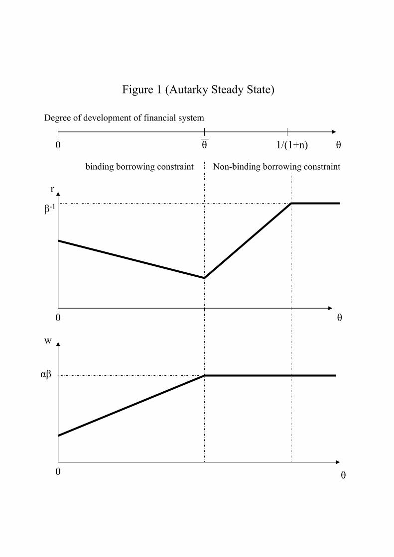
Figure 1 (Autarky Steady State)
Degree of development of financial system
0 θ
binding borrowing constraint
θ 1/(1+n)
0 θ
β-1
r
0 θ
w
αβ
Non-binding borrowing constraint

Figure 2 (Labor Market Equilibrium)
wt
rt
A
B
C
L’t= 0
L’t > 0
Figure 3 (Goods Market Equilibrium)
wt
rt
r*
D
E
F

Figure 4 (Short Run Equilibrium)
rt rt
rt rt
wt wt
wt wt
E
E
E
E
Type A: L’t > 0, rt > r*
Type B: L’t > 0, rt = r*
Type C: L’t = 0, rt = r*
Type D: L’t = 0, rt > r*
r*
r*r*
r*
w0
w0
w0
w0
r0
r0
Type A: L’t > 0, rt > r*

r
θ
r*
β-1
θ1 θ3θ2 θ4 θ5 θ6θ 1/(1+n)
r A
r A
Type A L’t > 0,rt > r*
Type B L’t > 0,rt = r*
Type C L’t = 0,rt = r*
Type D L’t = 0,rt > r*
Figure 5
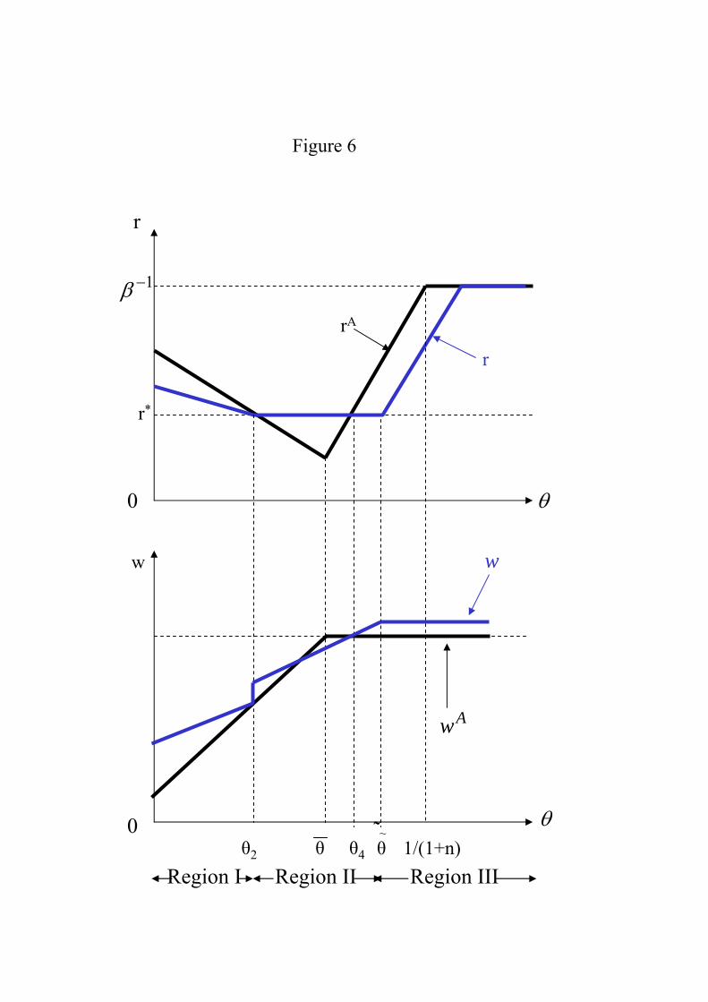
r
1−β
0 θ
θ0
Region I Region II Region III
Aw
w
r*
rA
r
w
θ2 θ θ4̃̃̃
1/(1+n)
Figure 6
~θ
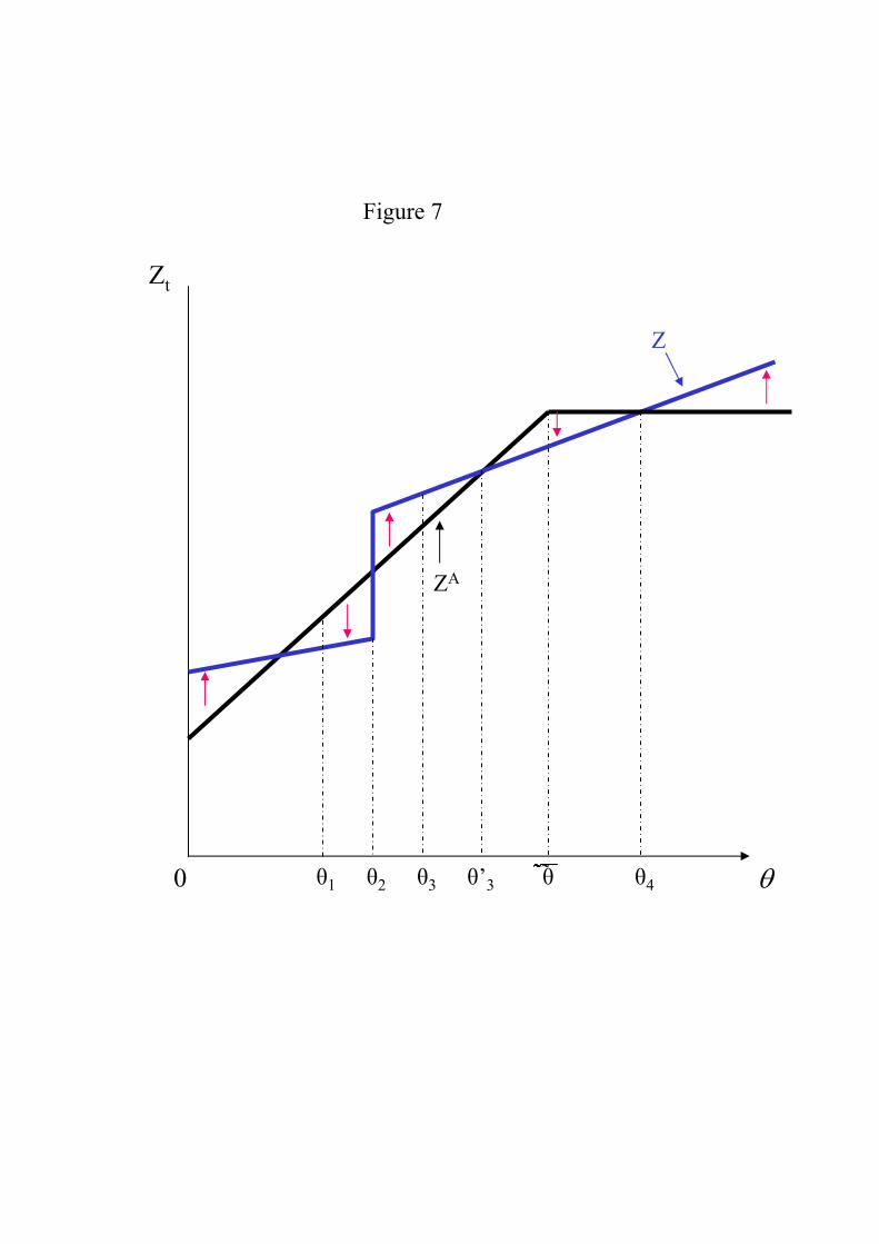
Zt
θ0
ZA
Z
θ2 θ3 ̃̃̃ ̃
Figure 7
θ1 θ θ4θ’3

Employment
tt0
Lt
Figure 8 (Dynamics of Employment - θ < θ2)
L’t
Lts

Employment
tt0
Lt
Figure 9a (Dynamics of Employment – θ2 < θ < θ3)
L’t
Lts
t1
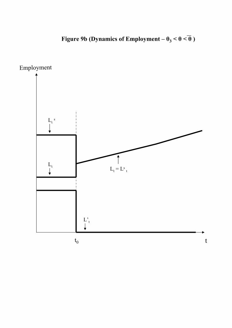
Employment
tt0
Lt
Figure 9b (Dynamics of Employment – θ3 < θ < θ )
L’t
Lts
Lt = Lst
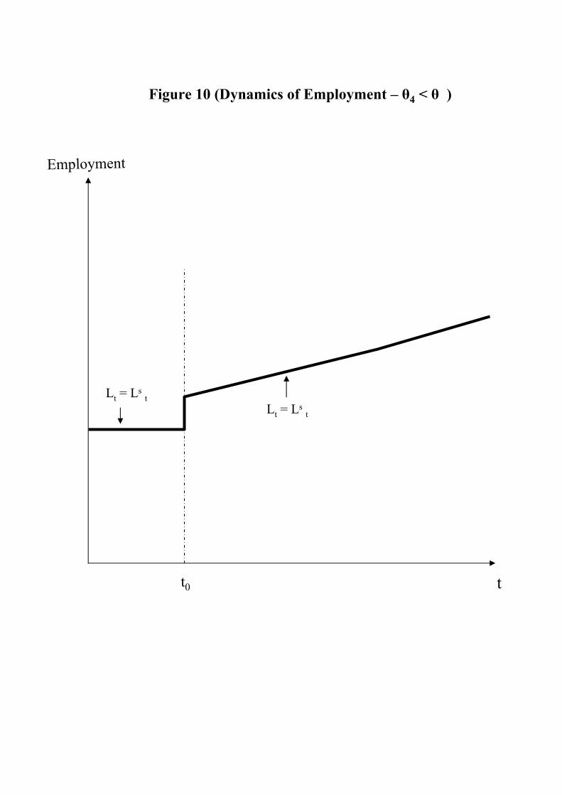
Employment
tt0
Figure 10 (Dynamics of Employment – θ4 < θ )
Lt = Lst
Lt = Lst

Employment
tt0
Lt
Figure 11 (Dynamics of Employment withand without government policy– θ2 < θ < θ3)
L’t
Lts
t1t’1
L’t
Lts
Lt
(stop subsidy)