Adjusting the valve boundary condition in Olkiluoto 1 load rejection test … · 2015-03-17 · 3...

RESEARCH REPORT No VTT-R-08574-07 9.10.2007

Adjusting the valve boundary condition in Olkiluoto 1 load rejection test calculated using TRAB-3D Authors Malla Seppälä

Confidentiality Public

3 (13)

Contents 1 Introduction 4

2 Models and solving methods in TRAB-3D 5

2.1 Neutronics 5 2.2 Thermal Hydraulics 6

3 Load rejection test 7

3.1 Test description 7 3.2 Calculation using TRAB-3D 8

4 New calculations 9

5 Results 10

6 Conclusions 12

References 13

4 (13)

1 Introduction

During the designing process of a nuclear power plant many kinds of safety

calculations are made to ensure the durability of the plant and to discover any

defects left unnoticed. One category of calculations is transient calculations in

which severe transient scenarios are studied in order to determine whether the

response of the reactor is in accordance with regulations. At the Technical

Research Center of Finland (VTT) three dimensional transient calculations are

performed using two programs, TRAB-3D and HEXTRAN, depending on the

geometry of the fuel assembly. Both programs have been developed at VTT. An

important part of developing a transient code that models nuclear reactors is the

validation of the program using international benchmarks or data from

experiments carried out on domestic nuclear reactors.

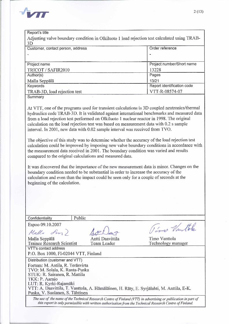
The objective of this study is to examine one of the validation calculations

performed on TRAB-3D, a load rejection test performed on the Olkiluoto 1

reactor in Finland in 1998, and to determine whether the calculation could be

enhanced using new, more detailed measurement data received from TVO in

2001. The original calculation was based on data with 0.2 s sample interval. In

the new data the sample interval is 0.02 s. The focus of the new calculation is on

a valve opening-closing mismatch that occurs during the first few seconds of the

test initiating a disturbance in the system pressure. The mismatch is modeled in

TRAB-3D with a boundary condition in the input. First the exact mismatch

values from the data are put to use in the boundary condition and the results are

assessed in respect to the original calculation to evaluate the importance of the

new data. Second the mismatch is adjusted to maximize the accuracy of

calculated pressure in respect of measured pressure during the first second of the

calculation. Last the accuracy of calculated pressure is maximized during first

three seconds of the calculation. The latter two calculations are performed to

determine the sensibility of the calculation regarding the mismatch.

5 (13)

2 Models and solving methods in TRAB-3D

In a nuclear reactor core the coupling of neutronics, heat transfer and thermal

hydraulics is very strongly present. It is therefore of vital important to describe

this phenomenon in the dynamic codes in order to gain a feasible model of the

core. At VTT coupled three dimensional transient codes have been developed,

validated and used since the mid eighties.

TRAB-3D [1, 2] is a stand-alone BWR dynamics code, whose core model is

based on the 3D hexagonal core model in HEXTRAN [3], and circuit and

system models are adopted from one-dimensional code TRAB [4]. TRAB-3D

can be applied to transient and accident analyses of boiling (BWR) and

pressurized water (PWR) reactors with rectangular fuel bundle geometry. The

code has been validated against international benchmarks and actual measured

data from real plant transients and it is in active use at VTT.

2.1 Neutronics

In TRAB-3D neutronics are modeled with two-group diffusion equations which

are solved by nodal expansion method in x-y-z-geometry. The nodal expansion

is based on the steady-state solution method for hexagonal core model in the

HEXBU-3D simulator. The basic principle of the solving method is the

decoupling of the diffusion equations, which is accomplished by separating the

equations using two spatial modes. The characteristic solutions of the spatial

modes construct the two group fluxes. There are two types of characteristic

solutions, asymptotic and transient. The fundamental, asymptotic mode is a

well-behaving function within a node and it can be approximated using

polynomial functions, whereas the transient mode has a large buckling in LWR

cores and therefore needs to be approximated by exponential functions. The

interaction of adjacent nodes is handled through continuity conditions at the

interfaces. The dynamic equations include six groups of delayed neutrons. [5]

A two-level iteration scheme is used to solve the nodal equations. In the inner

iteration only one unknown, the average fundamental mode, is determined. The

6 (13)

nodal flux shapes are enhanced in the outer iteration by recalculating the

coupling coefficients. Cross-sections are calculated using polynomial fittings to

coolant temperature, density and soluble boron density. Homogenized cross

sections are created with the CASMO-4 cell burnup code. [1]

2.2 Thermal Hydraulics

The thermal hydraulics model and its solution method are adopted from the one-

dimensional transient code TRAB. Flow channels are parallel and they are

connected freely to one or several fuel assemblies. The principal equations

represent the conservation of the masses of water and steam, respectively, total

enthalpy and total momentum. Additional equations for disequilibrium of

evaporation and condensation, slip and one- and two-phase friction can also be

utilized. Mass distribution through flow channels is determined from the

pressure balance in the core. The phase velocities are determined using slip ratio

or the drift-flux formalism. Properties of water and steam are calculated locally

as rational functions of pressure and enthalpy.

During the thermal hydraulic iteration one-dimensional heat transfer is

calculated for an average fuel rod in each fuel assembly. Fuel rod and cladding

are discretised with several radial mesh points and the calculations are

performed at equidistant axial elevations. Heat conduction is solved according to

Fourier’s law with temperature dependent thermal properties of fuel pellet, gas

gap and fuel cladding and with different heat transfer coefficients for different

hydraulic regimes.

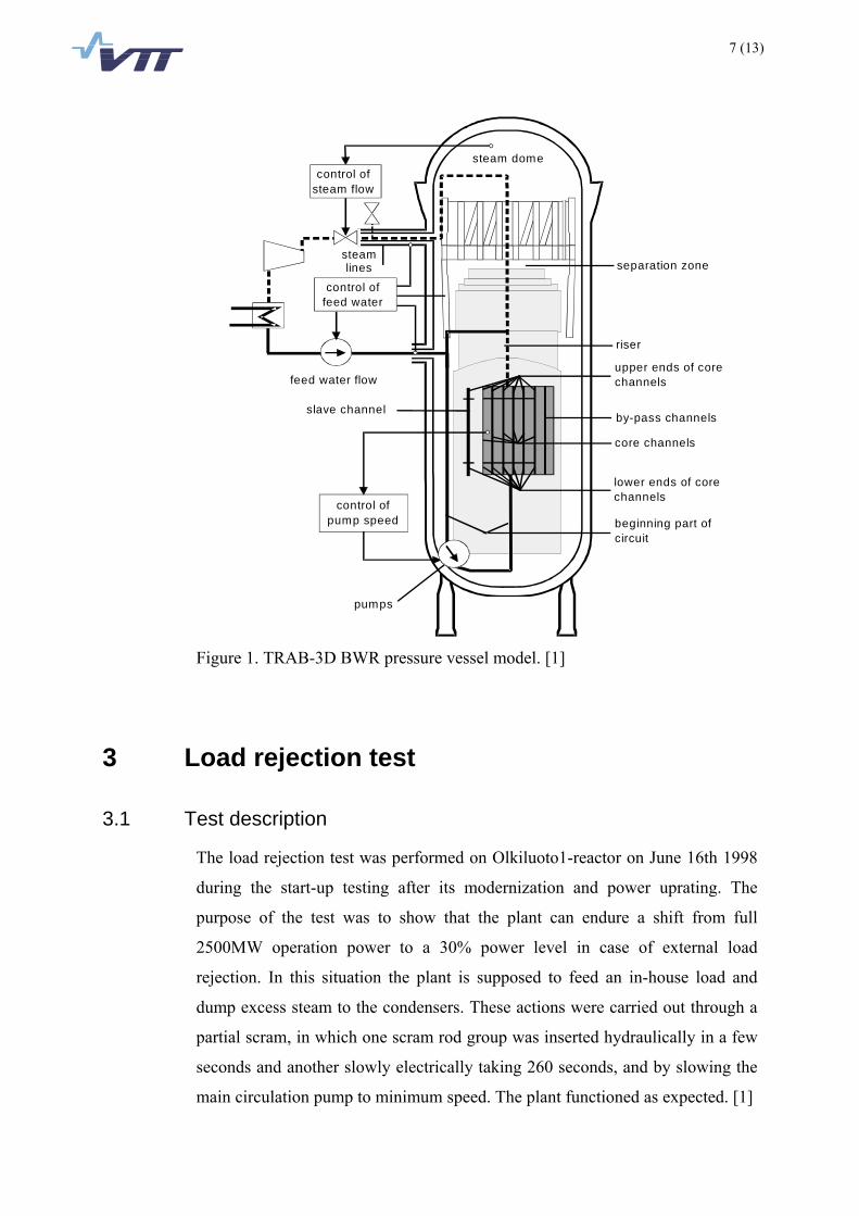
TRAB-3D includes a 1D model for BWR’s thermal hydraulics inside the

pressure vessel, as well as models for pumps, steam lines, and control systems.

The circuit components of TRAB-3D are shown in Figure 1. When TRAB-3D is

used for PWR transient calculations, it is coupled with a 1D thermal hydraulic

system code SMABRE for the hydraulic circuit. [1]

7 (13)

separation zone

riser

upper ends of corechannels

by-pass channels

beginning part ofcircuit

core channels

lower ends of corechannels

control offeed water

control ofpump speed

control ofsteam flow

pumps

slave channel

feed water flow

steam dome

steamlines

Figure 1. TRAB-3D BWR pressure vessel model. [1]

3 Load rejection test

3.1 Test description

The load rejection test was performed on Olkiluoto1-reactor on June 16th 1998

during the start-up testing after its modernization and power uprating. The

purpose of the test was to show that the plant can endure a shift from full

2500MW operation power to a 30% power level in case of external load

rejection. In this situation the plant is supposed to feed an in-house load and

dump excess steam to the condensers. These actions were carried out through a

partial scram, in which one scram rod group was inserted hydraulically in a few

seconds and another slowly electrically taking 260 seconds, and by slowing the

main circulation pump to minimum speed. The plant functioned as expected. [1]

8 (13)

The test offers excellent material for testing of 3D codes, because the transient is

asymmetric in the core and there are measurements from local power range

monitors available on several axial and radial locations in the core as well as

measurement values of bundle flows for several bundles.

At the initial stage of the test the plant was on 2500 MW operation power, the

turbine valves were open and the dump valves closed. At the beginning turbine

valves close and dump valves open. At the same time a partial scam takes place,

as one rod group is inserted hydraulically and another slowly. Feed water pumps

operate both under automatic control and under manual control by the operators.

The plant stabilized on a 30% house turbine operation power level. [6]

3.2 Calculation using TRAB-3D

Several modifications were initially done on TRAB-3D in order to calculate the

load rejection test. The first full core model on TRAB-3D was constructed, since

the partial scram was not half-core symmetric. The thermal hydraulic model was

altered to take into account the impact of the partial length Atrium fuel rods on

the flow geometry. A simple detector model was coded approximating local

power range monitors (LPRM) with averaging the thermal flux of the four nodes

adjacent to the detector. Average power range monitor (APRM) values are

calculated from 28 LPRM values. As the main object of the calculation was to

evaluate the capability of TRAB-3D to model 3D core phenomena, no

modifications were made on coolant circuit model or controller models. The

values of the feed water flow were set as transient boundary conditions because

of the manual operator actions during the test and due to the absence of feed

water controller in the present TRAB-3D input for TVO reactors. Feed water

enthalpy and pump speed were also used as boundary conditions. [7]

In the initial test measurement data the closing of the turbine valves and the

opening of the dump valves appeared simultaneous. After some test calculations,

a 0.05 s mismatch in the closing and opening of the valves was chosen due to

the relatively long sample interval 0.2 s, and the total time taken in opening and

closing the valves was fixed to 0.15 s. These values were also set as boundary

conditions for the calculation. The load rejection test was calculated for 400

9 (13)

seconds with TRAB-3D. Agreement with measured 3D time-dependent LPRM

data was good. [1, 8]

4 New calculations

In 2001 new, more specific measurement data of the load rejection with a 0.02 s

sample interval was received. The objective of this study is to determine

whether the accuracy of the calculation of the load rejection test could be

improved by imposing more detailed boundary conditions for the turbine and

dump valves in the beginning of the calculation. In addition, the sensitivity of

the calculation in respect of the opening and closing of valves was evaluated and

thereby the significance of the new data.

In the current TRAB-3D input opening and closing of valves is modeled by one

variable, which represents the fraction of openness of all the turbine and dump

valves. This is because in the present calculation the four steam lines are lumped

as one. Therefore, if no mismatch was related to the closing of the turbine valves

and the opening of the dump valves, the value of the valve variable, A2VAL1,

would stay one through the first few seconds of the calculation. In the initial

calculations the mismatch was modeled by a plateau between the beginning of

the closing of the turbine valves and the end of the opening of the dump valves,

shown in Figure 3. The constant value of the valve variable on the plateau was

determined by varying it and comparing the calculated pressure to measured

system pressure.

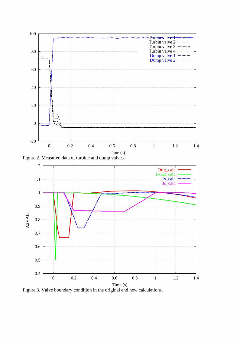
For the new calculation, the fraction of openness of the valves in the

measurement data was plotted to determine more detailed boundary conditions,

see Figure 2. In the new, exact boundary conditions mismatch is modeled the

same way as in the original calculation, by a plateau. The value of the valve

variable on the plateau was determined by comparing calculated and measured

pressures.

In order to evaluate the sensitivity of the calculation and to find out the optimal

mismatch values, the calculation was performed with varying valve boundary

10 (13)

condition values. The mismatch and time taken in opening and closing the

valves was varied freely, without paying any attention to the values gained from

measurement data. The accuracy of the calculated system pressure was chosen

as criterion for the quality of the boundary condition. At first only the first

second of the calculation was considered when comparing the pressures and

later first three seconds were taken into account.

Closer inspection of the new data revealed that the starting point of the

calculation needed to be readjusted in respect to the measured data to allow

comparison. The zero-time of the calculation was set to the beginning of the

valve opening/closing and the calculation started 0.1 seconds before it. In the

initial calculation, the zero-time of the calculation corresponded to 58.2 s in the

measured data. It was corrected to 58.28 s in accordance with the new data.

5 Results

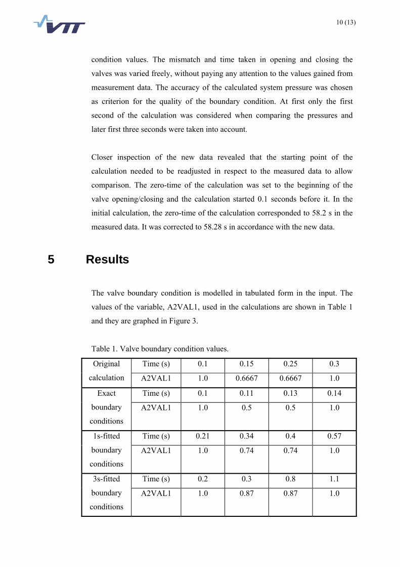
The valve boundary condition is modelled in tabulated form in the input. The

values of the variable, A2VAL1, used in the calculations are shown in Table 1

and they are graphed in Figure 3.

Table 1. Valve boundary condition values.

Time (s) 0.1 0.15 0.25 0.3 Original

calculation A2VAL1 1.0 0.6667 0.6667 1.0

Time (s) 0.1 0.11 0.13 0.14 Exact

boundary

conditions

A2VAL1 1.0 0.5 0.5 1.0

Time (s) 0.21 0.34 0.4 0.57 1s-fitted

boundary

conditions

A2VAL1 1.0 0.74 0.74 1.0

Time (s) 0.2 0.3 0.8 1.1 3s-fitted

boundary

conditions

A2VAL1 1.0 0.87 0.87 1.0

11 (13)

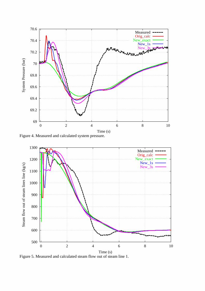
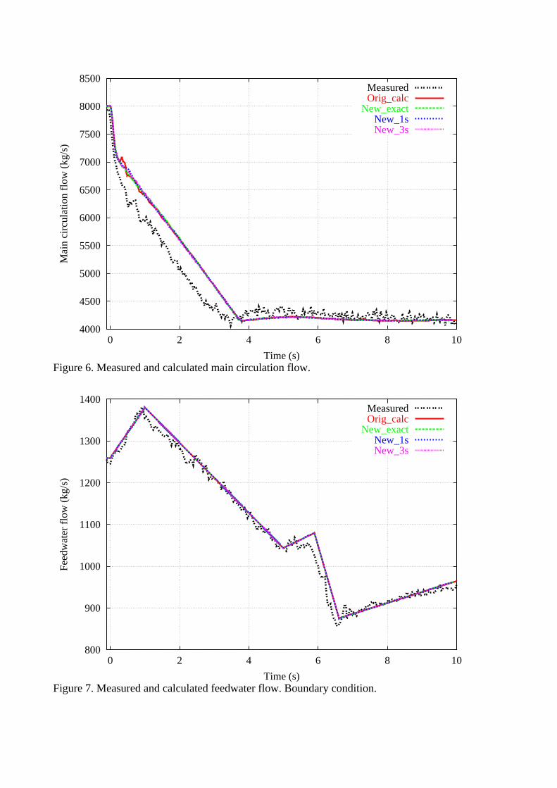
Figures of the most interesting variables, pressure, main circulation flow, steam

flow out of steam line and feed water flow are presented in Figures 4-7 for the

first ten seconds of the calculation for the different boundary conditions.

Measured data and data from original calculation are also graphed in the same

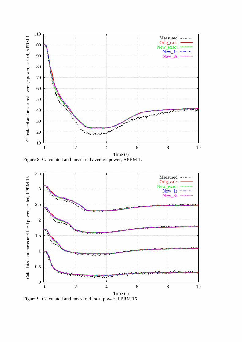
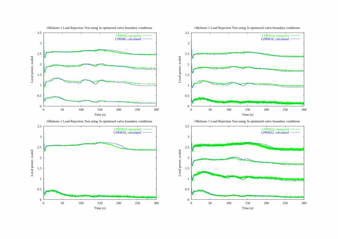
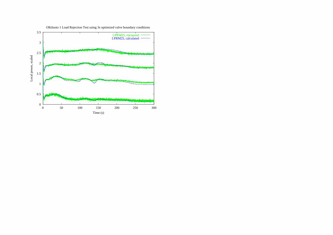
figures to allow comparison. In addition, results from a local power range

monitors (LPRM16) located near a hydraulic scram rod group at four heights

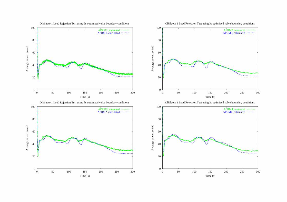
axially are shown in Figure 9 and results from an average power range monitor

(APRM1) based on 28 LPRM measurements in Figure 8. Relative LPRM values

are scaled with an arbitrary initial value to allow visualization of four axial

values in the same figure.

Examining system pressure in Figure 4 shows that the exact mismatch

determined from measured data is too rapid to create the rise in pressure

observed in the measured pressure in the beginning of the test. During the first

four seconds, the calculation performed using the exact boundary condition is

less accurate than the original calculations. For the calculation in which pressure

was optimized for the first second of the calculation, the calculated pressure is,

as expected, quite consistent with measured pressure for the first second and

therefore more accurate than the pressure in the original calculation. In the 3s

optimized calculation calculated pressure follows the measured pressure well for

almost three seconds. However, after four seconds all the calculated pressures

converge and no deviation can bee seen between the original calculation and

new calculations.

Steam flow out of steam line in Figure 5 shows differences between the

calculations for the first three seconds of the transient but little improvement can

be seen in its accuracy. In the other variables, the new calculations show little

variation from the original calculation.

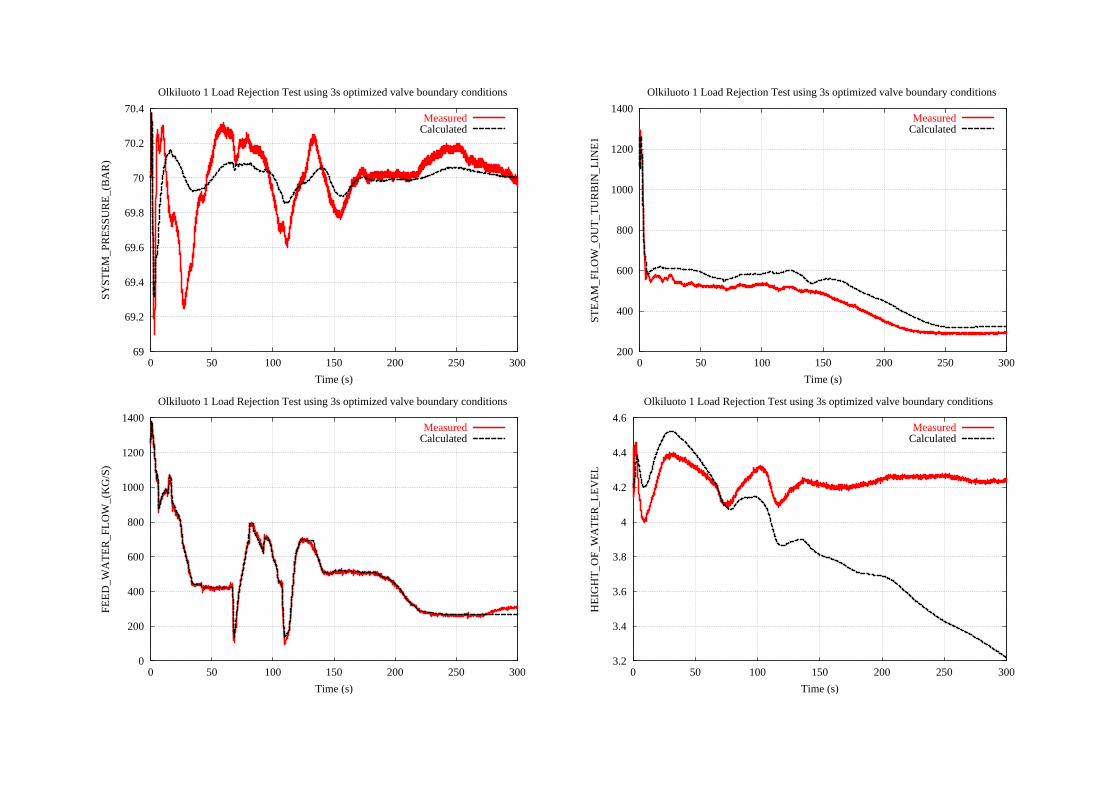
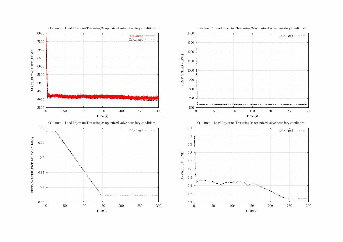
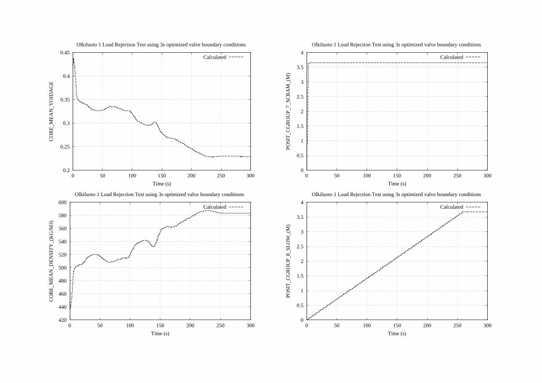
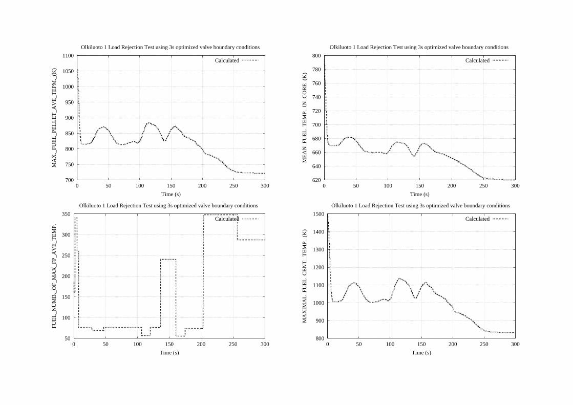
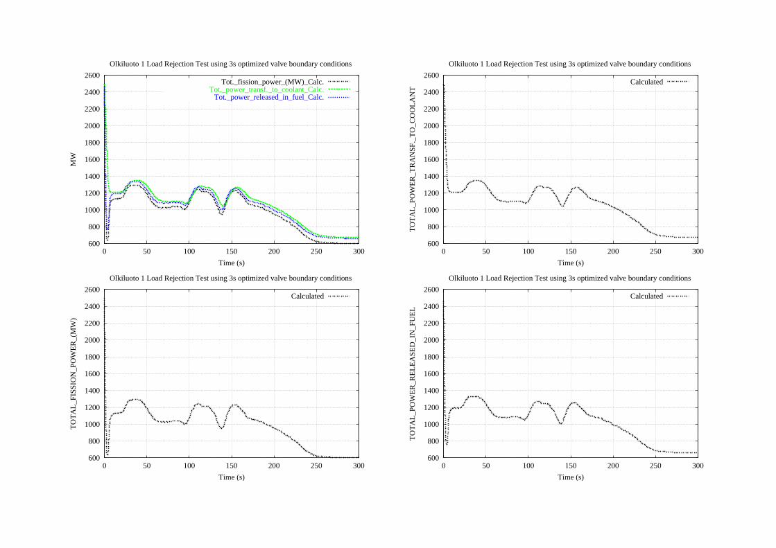
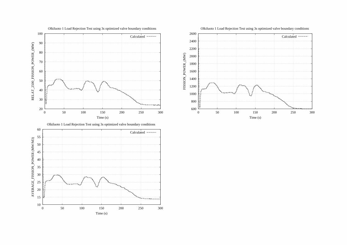
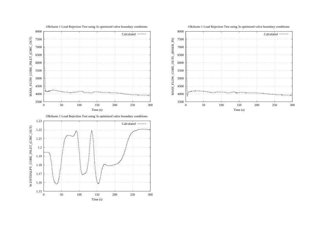
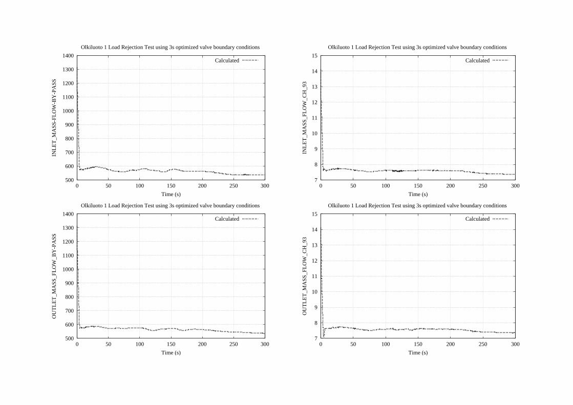
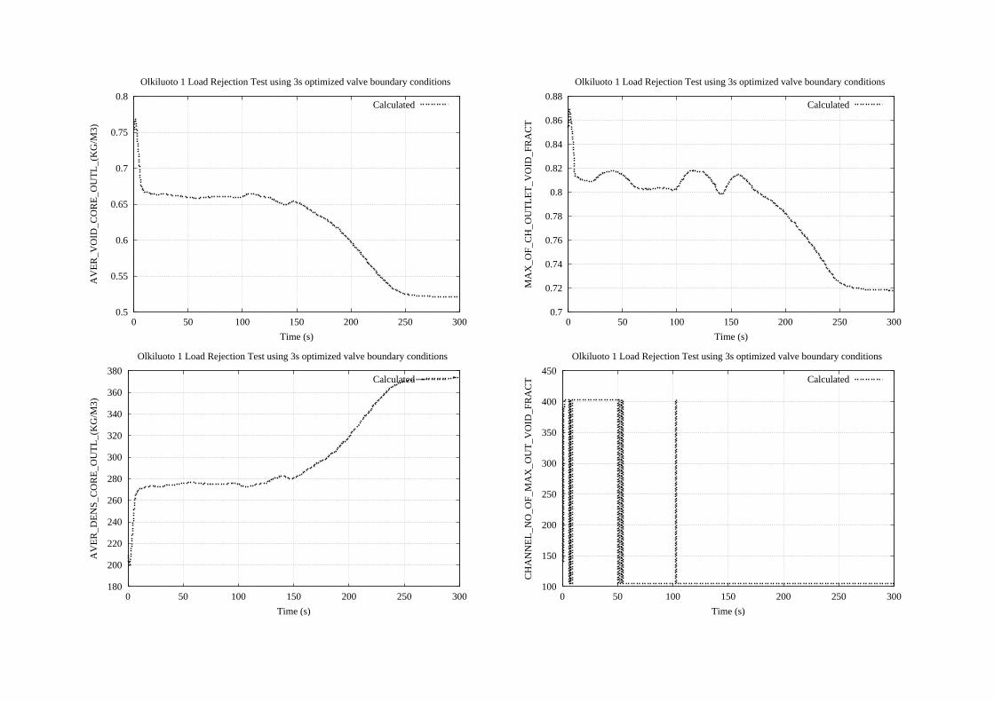
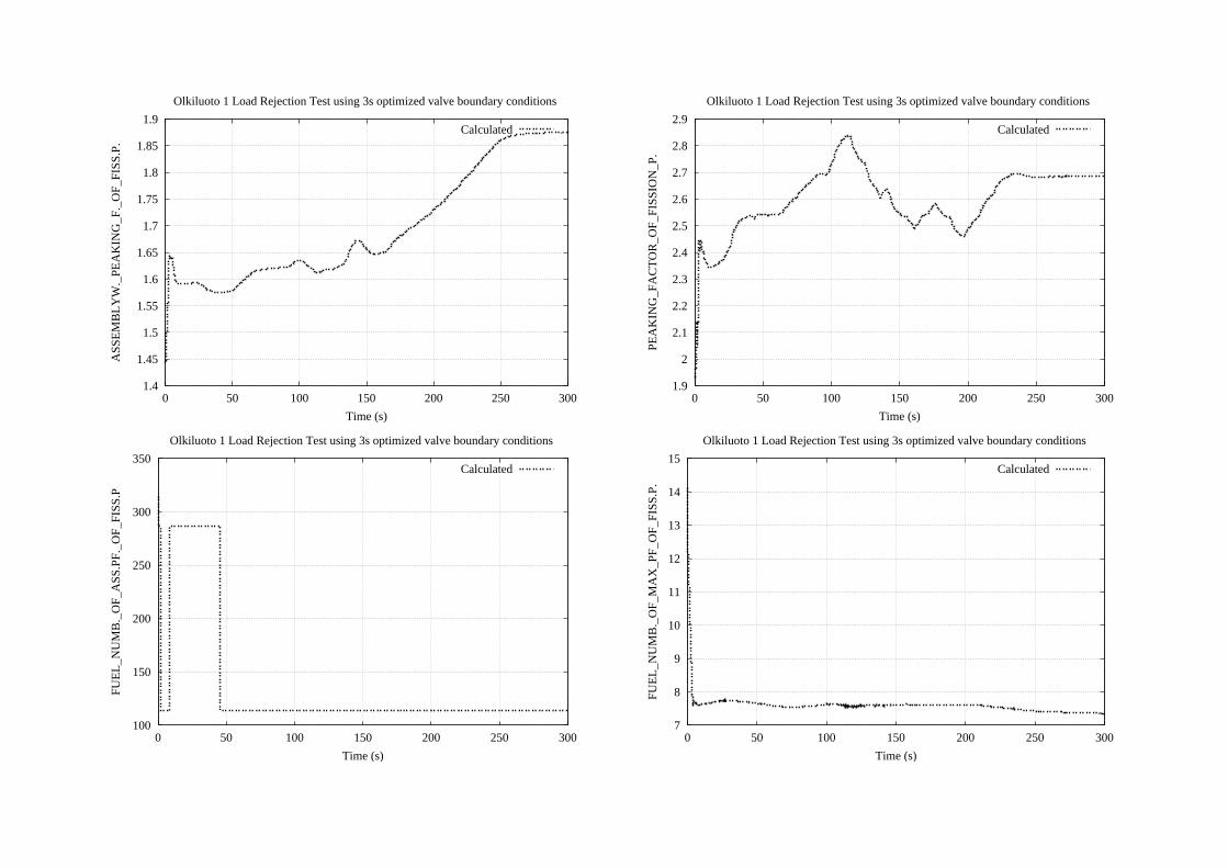
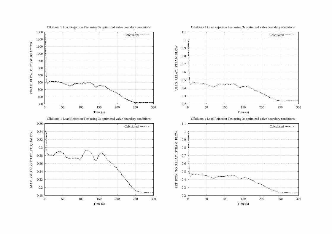
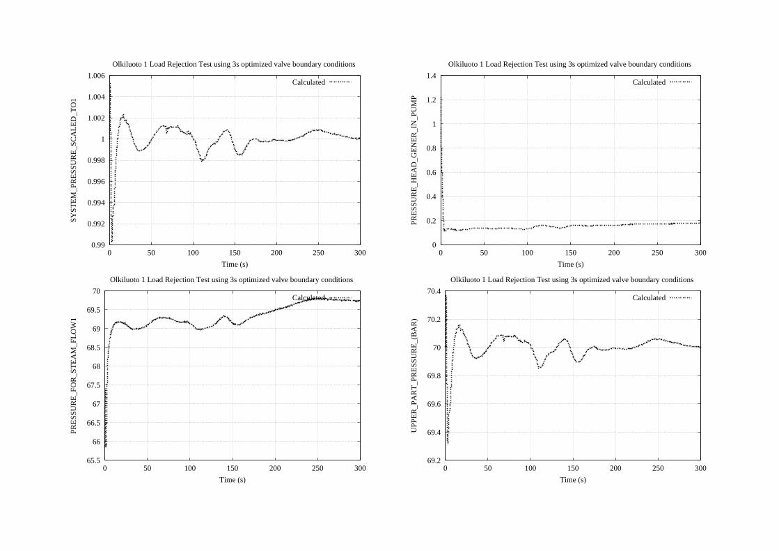
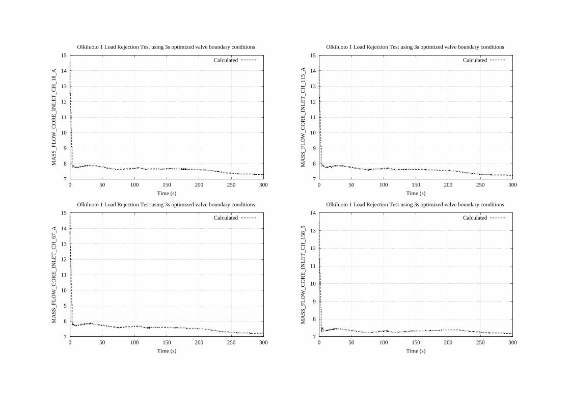
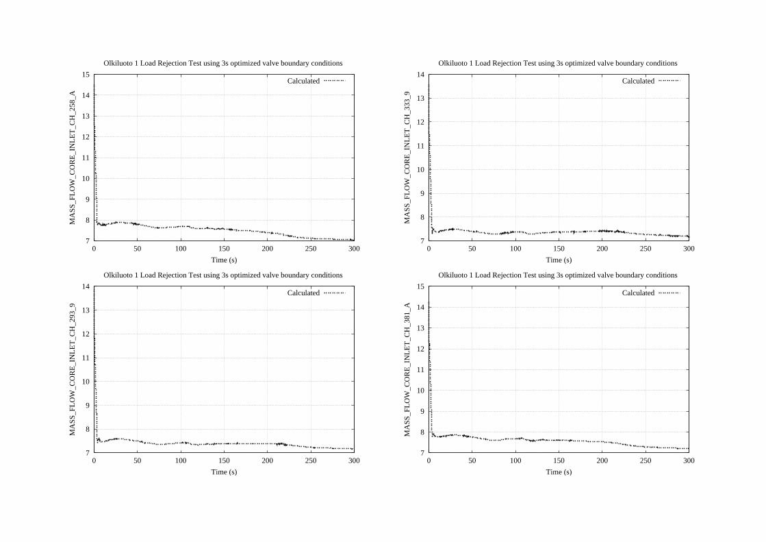
A longer 300 s calculation was performed using the last valve boundary

condition, in which pressure was optimized for three seconds. Figures of the

results are shown at the end of this report.

12 (13)

6 Conclusions

The objective of this study was to apply new, more detailed boundary conditions

to the transient calculation of the load rejection test performed in 1998 on

Olkiluoto 1 nuclear reactor. The exact boundary conditions for the valve

variable were determined from the new measurement data and they were used in

the calculation. In addition, the sensitivity of the calculation in respect of the

valve boundary condition was evaluated by trying to adjust calculated pressure

to measured pressure by varying the boundary condition freely. At first, only the

first second of the calculation was considered and second, first three seconds

were taken into account. The results are compared to the measured data as well

as the original calculation.

The results are shown in the figures at the end of this report. Using the exact

boundary conditions the mismatch appears to be too rapid in order to create the

rise in pressure observed in the beginning of the test. Therefore, the new, exact

boundary conditions do not enhance accuracy but rather impair it at the

beginning of the calculation. Overall, this has little impact on the calculation as

a whole. The calculations in which pressure was optimized for one and three

seconds, are somewhat more accurate than the original calculation at the

beginning, but their influence lasts no more than a couple of second. The impact

of the new boundary conditions is very little on other variables apart from

pressure and steam flow out of steam line.

As a conclusion, it can be summarized that the boundary conditions on the valve

variable are not critical concerning the load rejection test calculation. Some

enhancements can be attained during the first few seconds of the calculation, but

in order to do so the values of the valve variable must be changed substantially

from the one gained from measured data. Even when doing so, no effect is seen

after four seconds.

In the future, improvements on the calculation of the load rejection test could be

attained for example by adding a feed water controller model to the input. In the

13 (13)

present calculations height of water level is fairly accurate until 100 seconds.

After that, however, the absence of the controller model shows evidently.

References

[1] A. Daavittila, A. Hämäläinen & H. Räty, Transient and Fuel Performance

Analysis with VTT’s Coupled Code System, Mathematics and Computation,

Reactor Physics and Nuclear and Biological Applications, Avignon, France,

September 12-15, 2005

[2] Daavittila, A., Kaloinen, E., Kyrki-Rajamäki, R. & Räty, H. Validation of

TRAB-3D against Real BWR Plant Transients. In: International Meeting on “Best-

Estimate” Methods in Nuclear Installation Safety Analysis (BE-2000).

Washington, D.C., USA, 12-16 November, 2000 [CD-ROM]. La Grange Park:

American Nuclear Society, 2000. File Log40~54.pdf. ISBN 0-89448-658-6

[3] Kyrki-Rajamäki, R., HEXTRAN: VVER Reactor Dynamics Code for Three-

Dimensional Transients, In: Proceedings of the first Symposium of AER, Řež

near Prague, 23-28 September 1991. Budapest: KFKI Atomic Energy Research

Institute, 1991. Pp. 474-481.

[4] Rajamäki, M., TRAB, a transient analysis program for BWR, Part 1.

Principles. Helsinki 1980. Technical Research Centre of Finland, Nuclear

Engineering Laboratory, Report 45. 101 p + app. 9 p.

[5] Kaloinen, E. & Kyrki-Rajamäki, R., TRAB-3D, a new code for three-

dimensional reactor dynamics. CD-ROM Proceedings of ICONE-5, 5th

International Conference on Nuclear Engineering. "Nuclear Advances through

Global Cooperation". May 26-30 1997, Nice, France. Paper ICONE5-2197.

[6] Hanski, O., OL1 – koe 859, kuormanpudotuskoe, tulosraportti. TVO:n

muistio S03-KK-M-60/98. 17.6.1998. (in Finnish).

14 (13)

[7] Räty, H., TRAB-3D-Ohjelman Validointi Olkiluoto1 Kuormanpudotuskokeen

16.6.1998 Avulla, VTT Energy, Programme Document, ENE-PR-14/01.

[8] Daavittila, A, Räty, H., Reactor physics and dynamics (READY): Validation

of TRAB-3D. In: Kyrki-Rajamäki, Riitta & Puska, Eija-Karita (eds.) FINNUS The

Finnish Research Programme on Nuclear Power Plant Safety 1999-2002. Final

Report. Espoo: Technical Research Centre of Finland. Pp. 127 - 133. (VTT

Research Notes 2164). ISBN 951-38-6085-X, 951-38-6086-8.

-20

0

20

40

60

80

100

0 0.2 0.4 0.6 0.8 1 1.2 1.4

Time (s)

Turbin valve 1Turbin valve 2Turbin valve 3Turbin valve 4Dump valve 1Dump valve 2

Figure 2. Measured data of turbine and dump valves.

0.4

0.5

0.6

0.7

0.8

0.9

1

1.1

1.2

0 0.2 0.4 0.6 0.8 1 1.2 1.4

A2V

AL

1

Time (s)

Orig_calcExact_calc

1s_calc3s_calc

Figure 3. Valve boundary condition in the original and new calculations.

69

69.2

69.4

69.6

69.8

70

70.2

70.4

70.6

0 2 4 6 8 10

Syst

em P

ress

ure

(bar

)

Time (s)

MeasuredOrig_calc

New_exactNew_1sNew_3s

Figure 4. Measured and calculated system pressure.

500

600

700

800

900

1000

1100

1200

1300

0 2 4 6 8 10

Stea

m f

low

out

of

stea

m li

nes

line

(kg/

s)

Time (s)

MeasuredOrig_calc


Figure 5. Measured and calculated steam flow out of steam line 1.

4000

4500

5000

5500

6000

6500

7000

7500

8000

8500

0 2 4 6 8 10

Mai

n ci

rcul

atio

n fl

ow (

kg/s

)

Time (s)

MeasuredOrig_calc


Figure 6. Measured and calculated main circulation flow.

800

900

1000

1100

1200

1300

1400

0 2 4 6 8 10

Feed

wat

er f

low

(kg

/s)

Time (s)

MeasuredOrig_calc


Figure 7. Measured and calculated feedwater flow. Boundary condition.

10

20

30

40

50

60

70

80

90

100

110

0 2 4 6 8 10

Cal

cula

ted

and

mea

sure

d av

erag

e po

wer

, sca

led,

APR

M 1

Time (s)

MeasuredOrig_calc


Figure 8. Calculated and measured average power, APRM 1.

0

0.5

1

1.5

2

2.5

3

3.5

0 2 4 6 8 10

Cal

cula

ted

and

mea

sure

d lo

cal p

ower

, sca

led,

LPR

M 1

6

Time (s)

MeasuredOrig_calc


Figure 9. Calculated and measured local power, LPRM 16.

69

69.2

69.4

69.6

69.8

70

70.2

70.4

0 50 100 150 200 250 300

SYST

EM

_PR

ESS

UR

E_(

BA

R)

Time (s)

Olkiluoto 1 Load Rejection Test using 3s optimized valve boundary conditions

MeasuredCalculated

0

200

400

600

800

1000

1200

1400

0 50 100 150 200 250 300

FEE

D_W

AT

ER

_FL

OW

_(K

G/S

)

Time (s)


MeasuredCalculated

200

400

600

800

1000

1200

1400

0 50 100 150 200 250 300

STE

AM

_FL

OW

_OU

T_T

UR

BIN

_LIN

E1

Time (s)


MeasuredCalculated

3.2

3.4

3.6

3.8

4

4.2

4.4

4.6

0 50 100 150 200 250 300

HE

IGH

T_O

F_W

AT

ER

_LE

VE

L

Time (s)


MeasuredCalculated

3500

4000

4500

5000

5500

6000

6500

7000

7500

8000

0 50 100 150 200 250 300

MA

SS_F

LO

W_I

NT

O_P

UM

P

Time (s)


MeasuredCalculated

0.55

0.6

0.65

0.7

0.75

0.8

0 50 100 150 200 250 300

FEE

D_W

AT

ER

_EN

TH

AL

PY_(

MJ/

KG

)

Time (s)


Calculated

600

700

800

900

1000

1100

1200

1300

1400

0 50 100 150 200 250 300

PUM

P_SP

EE

D_(

RPM

)

Time (s)


Calculated

0.2

0.3

0.4

0.5

0.6

0.7

0.8

0.9

1

1.1

0 50 100 150 200 250 300

A2V

AL

1_ST

_LIN

E1

Time (s)


Calculated

0.2

0.25

0.3

0.35

0.4

0.45

0 50 100 150 200 250 300

CO

RE

_ME

AN

_VO

IDA

GE

Time (s)


Calculated

420

440

460

480

500

520

540

560

580

600

0 50 100 150 200 250 300

CO

RE

_ME

AN

_DE

NSI

TY

_(K

G/M

3)

Time (s)


Calculated

0

0.5

1

1.5

2

2.5

3

3.5

4

0 50 100 150 200 250 300

POSI

T_C

GR

OU

P_7_

SCR

AM

_(M

)

Time (s)


Calculated

0

0.5

1

1.5

2

2.5

3

3.5

4

0 50 100 150 200 250 300

POSI

T_C

GR

OU

P_8_

SLO

W_(

M)

Time (s)


Calculated

700

750

800

850

900

950

1000

1050

1100

0 50 100 150 200 250 300

MA

X._

FUE

L_P

EL

LE

T_A

VE

_TE

PM._

(K)

Time (s)


Calculated

50

100

150

200

250

300

350

0 50 100 150 200 250 300

FUE

L_N

UM

B._

OF_

MA

X_F

P_A

VE

_TE

MP.

Time (s)


Calculated

620

640

660

680

700

720

740

760

780

800

0 50 100 150 200 250 300

ME

AN

_FU

EL

_TE

MP.

_IN

_CO

RE

_(K

)

Time (s)


Calculated

800

900

1000

1100

1200

1300

1400

1500

0 50 100 150 200 250 300

MA

XIM

AL

_FU

EL

_CE

NT

._T

EM

P._(

K)

Time (s)


Calculated

600

800

1000

1200

1400

1600

1800

2000

2200

2400

2600

0 50 100 150 200 250 300

MW

Time (s)


Tot._fission_power_(MW)_Calc.Tot._power_transf._to_coolant_Calc.

Tot._power_released_in_fuel_Calc.

600

800

1000

1200

1400

1600

1800

2000

2200

2400

2600

0 50 100 150 200 250 300

TO

TA

L_F

ISSI

ON

_PO

WE

R_(

MW

)

Time (s)


Calculated

600

800

1000

1200

1400

1600

1800

2000

2200

2400

2600

0 50 100 150 200 250 300

TO

TA

L_P

OW

ER

_TR

AN

SF._

TO

_CO

OL

AN

T

Time (s)


Calculated

600

800

1000

1200

1400

1600

1800

2000

2200

2400

2600

0 50 100 150 200 250 300

TO

TA

L_P

OW

ER

_RE

LE

ASE

D_I

N_F

UE

L

Time (s)


Calculated

20

30

40

50

60

70

80

90

100

0 50 100 150 200 250 300

RE

LA

T_2

500_

FISS

ION

_PO

WE

R_(

MW

)

Time (s)


Calculated

10

15

20

25

30

35

40

45

50

55

60

0 50 100 150 200 250 300

AV

ER

AG

E_F

ISSI

ON

_PO

WE

R (

MW

/M3)

Time (s)


Calculated

600

800

1000

1200

1400

1600

1800

2000

2200

2400

2600

0 50 100 150 200 250 300

FISS

ION

_PO

WE

R_(

MW

)

Time (s)


Calculated

3500

4000

4500

5000

5500

6000

6500

7000

7500

8000

0 50 100 150 200 250 300

MA

SS_F

LO

W_C

OR

E_I

NL

ET

_(C

IRC

_OU

T)

Time (s)


Calculated

1.15

1.16

1.17

1.18

1.19

1.2

1.21

1.22

1.23

0 50 100 150 200 250 300

W.E

NT

HA

LPY

_CO

RE

_IN

LE

T_(

CIR

C_O

UT

)

Time (s)


Calculated

3500

4000

4500

5000

5500

6000

6500

7000

7500

8000

0 50 100 150 200 250 300

MA

SS_F

LO

W_C

OR

E_O

UT

L_(

RIS

ER

_IN

)

Time (s)


Calculated

500

600

700

800

900

1000

1100

1200

1300

1400

0 50 100 150 200 250 300

INL

ET

_MA

SS-F

LO

W-B

Y-P

ASS

Time (s)


Calculated

500

600

700

800

900

1000

1100

1200

1300

1400

0 50 100 150 200 250 300

OU

TL

ET

_MA

SS_F

LO

W_B

Y-P

ASS

Time (s)


Calculated

7

8

9

10

11

12

13

14

15

0 50 100 150 200 250 300

INL

ET

_MA

SS_F

LO

W_C

H_9

3

Time (s)


Calculated

7

8

9

10

11

12

13

14

15

0 50 100 150 200 250 300

OU

TL

ET

_MA

SS_F

LO

W_C

H_9

3

Time (s)


Calculated

0.5

0.55

0.6

0.65

0.7

0.75

0.8

0 50 100 150 200 250 300

AV

ER

_VO

ID_C

OR

E_O

UT

L_(

KG

/M3)

Time (s)


Calculated

180

200

220

240

260

280

300

320

340

360

380

0 50 100 150 200 250 300

AV

ER

_DE

NS_

CO

RE

_OU

TL

_(K

G/M

3)

Time (s)


Calculated

0.7

0.72

0.74

0.76

0.78

0.8

0.82

0.84

0.86

0.88

0 50 100 150 200 250 300

MA

X_O

F_C

H_O

UT

LE

T_V

OID

_FR

AC

T

Time (s)


Calculated

100

150

200

250

300

350

400

450

0 50 100 150 200 250 300

CH

AN

NE

L_N

O_O

F_M

AX

_OU

T_V

OID

_FR

AC

T

Time (s)


Calculated

1.4

1.45

1.5

1.55

1.6

1.65

1.7

1.75

1.8

1.85

1.9

0 50 100 150 200 250 300

ASS

EM

BL

YW

._PE

AK

ING

_F._

OF_

FISS

.P.

Time (s)


Calculated

100

150

200

250

300

350

0 50 100 150 200 250 300

FUE

L_N

UM

B._

OF_

ASS

.PF.

_OF_

FISS

.P

Time (s)


Calculated

1.9

2

2.1

2.2

2.3

2.4

2.5

2.6

2.7

2.8

2.9

0 50 100 150 200 250 300

PEA

KIN

G_F

AC

TO

R_O

F_FI

SSIO

N_P

.

Time (s)


Calculated

7

8

9

10

11

12

13

14

15

0 50 100 150 200 250 300

FUE

L_N

UM

B._

OF_

MA

X_P

F_O

F_FI

SS.P

.

Time (s)


Calculated

300

400

500

600

700

800

900

1000

1100

1200

1300

0 50 100 150 200 250 300

STE

AM

_FL

OW

_OU

T_O

F_R

EA

CT

OR

Time (s)


Calculated

0.18

0.2

0.22

0.24

0.26

0.28

0.3

0.32

0.34

0.36

0 50 100 150 200 250 300

MA

X._

OF_

CH

_OU

TL

ET

_ST

_QU

AL

ITY

Time (s)


Calculated

0.2

0.3

0.4

0.5

0.6

0.7

0.8

0.9

1

1.1

0 50 100 150 200 250 300

USE

D_R

EL

AT

._ST

EA

M_F

LO

W

Time (s)


Calculated

0.2

0.3

0.4

0.5

0.6

0.7

0.8

0.9

1

1.1

0 50 100 150 200 250 300

SET

_PO

IN_T

O_R

EL

AT

._ST

EA

M_F

LO

W

Time (s)


Calculated

0.99

0.992

0.994

0.996

0.998

1

1.002

1.004

1.006

0 50 100 150 200 250 300

SYST

EM

_PR

ESS

UR

E_S

CA

LE

D_T

O1

Time (s)


Calculated

65.5

66

66.5

67

67.5

68

68.5

69

69.5

70

0 50 100 150 200 250 300

PRE

SSU

RE

_FO

R_S

TE

AM

_FL

OW

1

Time (s)


Calculated

0

0.2

0.4

0.6

0.8

1

1.2

1.4

0 50 100 150 200 250 300

PRE

SSU

RE

_HE

AD

_GE

NE

R_I

N_P

UM

P

Time (s)


Calculated

69.2

69.4

69.6

69.8

70

70.2

70.4

0 50 100 150 200 250 300

UPP

ER

_PA

RT

_PR

ESS

UR

E_(

BA

R)

Time (s)


Calculated

7

8

9

10

11

12

13

14

15

0 50 100 150 200 250 300

MA

SS_F

LO

W_C

OR

E_I

NL

ET

_CH

_18_

A

Time (s)


Calculated

7

8

9

10

11

12

13

14

15

0 50 100 150 200 250 300

MA

SS_F

LO

W_C

OR

E_I

NL

ET

_CH

_67_

A

Time (s)


Calculated

7

8

9

10

11

12

13

14

15

0 50 100 150 200 250 300

MA

SS_F

LO

W_C

OR

E_I

NL

ET

_CH

_115

_A

Time (s)


Calculated

7

8

9

10

11

12

13

14

0 50 100 150 200 250 300

MA

SS_F

LO

W_C

OR

E_I

NL

ET

_CH

_158

_9

Time (s)


Calculated

7

8

9

10

11

12

13

14

15

0 50 100 150 200 250 300

MA

SS_F

LO

W_C

OR

E_I

NL

ET

_CH

_258

_A

Time (s)


Calculated

7

8

9

10

11

12

13

14

0 50 100 150 200 250 300

MA

SS_F

LO

W_C

OR

E_I

NL

ET

_CH

_293

_9

Time (s)


Calculated

7

8

9

10

11

12

13

14

0 50 100 150 200 250 300

MA

SS_F

LO

W_C

OR

E_I

NL

ET

_CH

_333

_9

Time (s)


Calculated

7

8

9

10

11

12

13

14

15

0 50 100 150 200 250 300

MA

SS_F

LO

W_C

OR

E_I

NL

ET

_CH

_381

_A

Time (s)


Calculated

0

20

40

60

80

100

0 50 100 150 200 250 300

Ave

rage

pow

er, s

cale

d

Time (s)


APRM1, measuredAPRM1, calculated

0

20

40

60

80

100

0 50 100 150 200 250 300

Ave

rage

pow

er, s

cale

d

Time (s)



0

20

40

60

80

100

0 50 100 150 200 250 300

Ave

rage

pow

er, s

cale

d

Time (s)



0

20

40

60

80

100

0 50 100 150 200 250 300

Ave

rage

pow

er, s

cale

d

Time (s)



0

0.5

1

1.5

2

2.5

3

3.5

0 50 100 150 200 250 300

Loc

al p

ower

, sca

led

Time (s)


LPRM6, measuredLPRM6, calculated

0

0.5

1

1.5

2

2.5

3

3.5

0 50 100 150 200 250 300

Loc

al p

ower

, sca

led

Time (s)



0

0.5

1

1.5

2

2.5

3

3.5

0 50 100 150 200 250 300

Loc

al p

ower

, sca

led

Time (s)



0

0.5

1

1.5

2

2.5

3

3.5

0 50 100 150 200 250 300

Loc

al p

ower

, sca

led

Time (s)



0

0.5

1

1.5

2

2.5

3

3.5

0 50 100 150 200 250 300

Loc

al p

ower

, sca

led

Time (s)



Adjusting the valve boundary condition in Olkiluoto 1 load rejection test … · 2015-03-17 · 3...

Documents

Transcript of Adjusting the valve boundary condition in Olkiluoto 1 load rejection test … · 2015-03-17 · 3...