ADDITIVE MANUFACTURING OF SHORT-FIBER COMPOSITES VIA ...

ADDITIVE MANUFACTURING OF SHORT-FIBER COMPOSITES VIA

STEREOLITHOGRAPHY

A Thesis

Submitted to the Graduate Faculty

of the

North Dakota State University

of Agriculture and Applied Science

By

Patrick Glenn Simpson

In Partial Fulfillment of the Requirements

for the Degree of

MASTER OF SCIENCE

Major Department:

Mechanical Engineering

December 2018

Fargo, North Dakota

North Dakota State University

Graduate School

Title

Additive Manufacturing of Short-Fiber Composites via Stereolithography

By

Patrick Glenn Simpson

The Supervisory Committee certifies that this disquisition complies with North Dakota

State University’s regulations and meets the accepted standards for the degree of

MASTER OF SCIENCE

SUPERVISORY COMMITTEE:

Dr. Chad Ulven

Chair

Dr. Dilpreet Bajwa

Dr. Dean Webster

Approved:

12/7/2018 Dr. Alan R. Kallmeyer

Date Department Chair

iii

ABSTRACT

The effectiveness of using a dual curing system, consisting of a photo and thermal

initiator, for the additive manufacturing of carbon fiber short-fiber composites via

stereolithography was investigated. The necessary processing parameters were developed that

resulted in successful printing and curing of composites at a 5% fiber volume. The effects of

layer height and print orientation of the short-fiber composites were evaluated for their effect on

the material properties. There was no increase in the flexural modulus or fracture toughness, and

a decrease the tensile and flexural strength of the short-fiber composites produced. This was

found to be due to weak fiber/matrix interfacial properties, a wide fiber length distribution, and

issues with fiber volume consistency. An increase in the tensile modulus was seen and that it

could be manipulated with adjustments to layer height and part orientation.

iv

ACKNOWLEDGEMENTS

I would like to thank the Army Research Laboratory for provide the funding for this

research. I would like to thank my adviser, Dr. Chad Ulven, for providing thoughtful discussions,

and guidance during this research. I would also like to thank my committee members, Dr. Dean

Webster and Dr. Dilpreet Bajwa, for their advice during this research.

v

TABLE OF CONTENTS

ABSTRACT ................................................................................................................................... iii

ACKNOWLEDGEMENTS ........................................................................................................... iv

LIST OF TABLES ....................................................................................................................... viii

LIST OF FIGURES ....................................................................................................................... xi

LIST OF APPENDIX TABLES .................................................................................................. xiv

LIST OF APPENDIX FIGURES ............................................................................................... xvii

1. INTRODUCTION ...................................................................................................................... 1

2. BACKGROUND ........................................................................................................................ 3

2.1. Stereolithography ......................................................................................................... 3

2.1.1. Printing Methods ............................................................................................... 3

2.1.2. Printing Materials .............................................................................................. 4

2.1.3. Isotropic Material Properties ............................................................................. 5

2.2. Short-Fiber Composites ............................................................................................... 6

2.3. Additive Manufacturing of Short-Fiber Composites ................................................... 9

2.3.1. FDM Produced Short-Fiber Composites ........................................................... 9

2.3.2. SLA Produced Composites.............................................................................. 12

2.4. Dual Cure Resin System ............................................................................................ 15

3. OBJECTIVES ........................................................................................................................... 16

4. RESEARCH METHODOLOGY ............................................................................................. 17

4.1. Materials and Equipment ........................................................................................... 17

4.1.1. Moai Printer ..................................................................................................... 17

4.1.2. Photopolymer Resins ....................................................................................... 18

4.1.3. Carbon Fiber .................................................................................................... 18

4.1.4. Thermal Initiators ............................................................................................ 20

vi

4.2. Sample Manufacturing ............................................................................................... 21

4.2.1. Resin Manufacturing ....................................................................................... 21

4.2.2. Processing Parameters for 3D Printing Parts................................................... 22

4.2.3. Post-Processing of 3D Printed Parts ................................................................ 25

4.3. Material Property Characterization of 3D Printed Composites ................................. 28

4.3.1. Thermal Initiator Selection .............................................................................. 28

4.3.2. Viscosity Testing ............................................................................................. 29

4.3.3. Tensile Testing ................................................................................................ 31

4.3.4. Flexural Testing ............................................................................................... 34

4.3.5. Fracture Toughness Testing ............................................................................ 36

4.3.6. Fiber Volume Consistency .............................................................................. 38

4.3.7. Composite Void Content ................................................................................. 40

4.3.8. Post-Cure Shrinkage ........................................................................................ 41

4.3.9. Scanning Electron Microscopy........................................................................ 42

5. RESULTS AND DISCUSSION ............................................................................................... 43

5.1. UV Cured Short Fiber Reinforced Composites ......................................................... 43

5.1.1. Tensile Testing ................................................................................................ 43

5.2. Dual Cured Short Fiber Reinforced Composite ......................................................... 45

5.2.1. Thermal Initiator Evaluation ........................................................................... 45

5.2.2. Carbon Fiber Evaluation.................................................................................. 50

5.2.3. Fiber Volume Consistency and Porosity ......................................................... 56

5.2.4. Material Characterization ................................................................................ 59

6. CONCLUSIONS AND RECOMMENDATIONS ................................................................. 122

6.1. Conclusions .............................................................................................................. 122

6.2. Future Recommendations ........................................................................................ 126

vii

REFERENCES ........................................................................................................................... 128

APPENDIX A. EXPERIMENTAL DATA ................................................................................ 134

APPENDIX B. STATISTICAL DATA ...................................................................................... 144

viii

LIST OF TABLES

Table Page

2.1: Mechanical properties of commercially available SLA resins. ............................................... 5

4.1: Peopoly resin constituents [9]. ............................................................................................... 18

4.2: Mechanical properties of various carbon fiber [41]............................................................... 19

4.3: Toray T-700 fiber properties [42]. ......................................................................................... 20

4.4: Carbiso MF SM45R-100 fiber properties [43]. ..................................................................... 20

4.5 Thermal initiators to be investigated for a dual cure resin system. ........................................ 21

4.6: Tensile testing experimental variables. .................................................................................. 32

4.7: Tensile testing test matrix. ..................................................................................................... 33

4.8: Qcritical for Tukey HSD tension testing. .................................................................................. 34

4.9: Flexural testing experimental variables. ................................................................................ 35

4.10: Flexural testing test matrix. ................................................................................................. 36

4.11: Fracture toughness testing experimental variables. ............................................................. 37

4.12: Fracture toughness testing test matrix. ................................................................................ 38

4.13: Qcritical for Tukey HSD fracture toughness testing. .......................................................... 38

4.14: Post-cure shrinkage test samples. ........................................................................................ 41

5.1: Tensile testing results for UV cured at 5% Vf carbon fiber. .................................................. 44

5.2: Thermal initiator solubility and stability testing. ................................................................... 46

5.3: Thermal initiator onset temperature from DSC curves. ......................................................... 47

5.4: Viscosity of composite resins. ............................................................................................... 47

5.5: Printer settings changed for printing with carbon fiber resin. ............................................... 51

5.6: Tensile testing results for Carbiso carbon fiber. .................................................................... 52

5.7: Tensile testing results for Toray T-700 carbon fiber. ............................................................ 54

5.8: Post-curing study for carbon fiber composite (Luperox P). .................................................. 54

ix

5.9: Post-curing study for carbon fiber composite (Cumene Hydroperoxide). ............................. 55

5.10: Summarized fiber volume consistency results for flexural samples.................................... 56

5.11: Density and void content of composite samples. ................................................................. 58

5.12: Sample identification guide. ................................................................................................ 60

5.13: Summarized tensile testing results. ...................................................................................... 63

5.14: Volumetric shrinkage (%) of post-cured samples................................................................ 66

5.15: Statistical analysis groups. ................................................................................................... 72

5.16: ANOVA summary for Young's modulus in 0º print orientation. ........................................ 72

5.17: Tukey HSD results for Young's modulus in 0º print orientation. ........................................ 74

5.18: ANOVA summary for Young's modulus in 90º print orientation. ...................................... 75

5.19: ANOVA summary for Young's modulus printed at 100 μm layer height. .......................... 76

5.20: Tukey HSD results for Young's modulus printed at 100 μm layer height. .......................... 78

5.21: ANOVA summary for Young's modulus printed at 50 μm layer height. ............................ 78

5.22: Tukey HSD results for Young's modulus printed at 50 μm layer height. ............................ 80

5.23: ANOVA summary for tensile strength in 0º print orientation. ............................................ 81

5.24: Tukey HSD results for tensile strength in 0º print orientation............................................. 82

5.25: ANOVA summary for tensile strength in 90º print orientation. .......................................... 82

5.26: Tukey HSD results for tensile strength in 90º print orientation........................................... 84

5.27: ANOVA summary for tensile strength printed at 100 μm layer height. .............................. 84

5.28: Tukey HSD results for tensile strength printed at 100 μm layer height. ............................. 86

5.29: ANOVA summary for tensile strength at 50 μm layer height. ............................................ 86

5.30: Tukey HSD results for tensile strength printed at 50 μm layer height. ............................... 88

5.31: Summarized flexural testing results. .................................................................................... 91

5.32: ANOVA summary for flexural modulus in 0º print orientation. ......................................... 93

5.33: Tukey HSD results for flexural modulus in 0º print orientation. ......................................... 95

x

5.34: ANOVA summary for flexural modulus in 90º print orientation. ....................................... 95

5.35: Tukey HSD results for flexural modulus in 90º print orientation. ....................................... 97

5.36: ANOVA summary for flexural modulus printed at 100 μm layer height. ........................... 97

5.37: Tukey HSD results for flexural modulus printed at 100 μm layer height. .......................... 99

5.38: ANOVA summary for flexural modulus printed at 50 μm layer height. ............................. 99

5.39: Tukey HSD results for flexural modulus printed at 50 μm layer height. .......................... 101

5.40: ANOVA summary for flexural strength in 0º print orientation. ........................................ 101

5.41: Tukey HSD results for flexural strength in 0º print orientation......................................... 103

5.42: ANOVA summary for flexural strength in 90º print orientation. ...................................... 104

5.43: Tukey HSD results for flexural strength in 90º print orientation....................................... 105

5.44: ANOVA summary for flexural strength printed at 100 μm layer height. .......................... 106

5.45: Tukey HSD results for flexural strength printed at 100 μm layer height. ......................... 107

5.46: ANOVA summary for flexural strength at 50 μm layer height. ........................................ 108

5.47: Tukey HSD results for flexural strength printed at 50 μm layer height. ........................... 110

5.48: Summarized fracture testing results. .................................................................................. 113

5.49: ANOVA summary for fracture toughness in the 0º print orientation. ............................... 115

5.50: ANOVA summary for fracture toughness in the 90º print orientation. ............................. 116

5.51: ANOVA summary for fracture toughness of 100 μm layer height. .................................. 118

5.52: ANOVA summary for fracture toughness of 50 μm layer height. .................................... 120

xi

LIST OF FIGURES

Figure Page

2.1: Bottom-up SLA printer. ........................................................................................................... 4

2.2: Schematic of layers SLA printing process. .............................................................................. 6

2.3: Dual curing system. ............................................................................................................... 15

3.1: Effects of layer height on fiber orientation. ........................................................................... 16

4.1: Moai SLA printer. .................................................................................................................. 18

4.2: Before (left) and after (right) support material being added. ................................................. 23

4.3: Cura slicing software. ............................................................................................................ 24

4.4: Sample long axis orientation.................................................................................................. 25

4.5: UV cure oven. ........................................................................................................................ 26

4.6: Post-curing oven. ................................................................................................................... 27

4.7: Surface defects from support removal. .................................................................................. 27

4.8: Removal of supports and surface effects. .............................................................................. 28

4.9: AR-G2 rheometer. ................................................................................................................. 30

4.10: Tensile testing specimen (all dimensions in mm). ............................................................... 31

4.11: Flexural testing specimen (all dimensions in mm). ............................................................. 35

4.12: SENB specimen for fracture testing (all dimensions in mm). ............................................. 37

4.13: Burn off sample testing areas............................................................................................... 39

4.14: Thermolyne muffle furnace. ................................................................................................ 40

4.15: Void content and density test specimen (all dimensions mm)............................................. 41

5.1: Representative stress-strain curves. ....................................................................................... 44

5.2: Viscosity testing with for shear rate from 1 s-1 to 25 s-1. ....................................................... 48

5.3: Viscosity testing with for shear rate from 1 s-1 to 100 s-1. ..................................................... 49

5.4: Milled Toray T-700 fiber length distribution. ....................................................................... 50

xii

5.5: SEM imaging of fracture surface of Carbiso fiber composite. .............................................. 53

5.6: Cracks in cumene hydroperoxide post-cured specimens. ...................................................... 56

5.7: Tensile strength results for 0º print orientation...................................................................... 61

5.8: Young's modulus results for 0º print orientation. .................................................................. 61

5.9: Tensile stregnth results for 90º print orientation.................................................................... 62

5.10: Young's modulus results for 90º print orientation. .............................................................. 62

5.11: Fracture surface of CF50-0 (A) X200 and (B) X250 magnification. .................................. 64

5.12: Fracture surface of (A) CF100-90 and (B) CF50-90 specimens. ........................................ 65

5.13: Surface cracking from thermal curing. ................................................................................ 66

5.14: M100-90 fracture surface at (A) X500 and (B) X1000 magnification. ............................... 67

5.15: M50-90 fracture surface at (A) X500 and (B) X1000 magnification. ................................. 68

5.16: LP100-0 fracture surface at (A) X500 and (B) X1000 magnification. ................................ 69

5.17: Cracks in CF50-90 sample from printing. ........................................................................... 70

5.18: Examples of CF50-90 print failures..................................................................................... 70

5.19: Box plot of ANOVA results for Young's modulus in 0º print orientation. ......................... 73

5.20: Box plot of ANOVA results for Young's modulus in 90º print orientation. ....................... 75

5.21: Box plot of ANOVA results for Young's modulus printed at 100 μm layer height. ........... 77

5.22: Box plot of ANOVA results for Young's modulus printed at 50 μm layer height. ............. 79

5.23: Box plot of ANOVA results for tensile strength in 0º print orientation. ............................. 81

5.24: Box plot of ANOVA results for tensile strength in 90º print orientation. ........................... 83

5.25: Box plot of ANOVA results for tensile strength printed at 100 μm layer height. ............... 85

5.26: Box plot of ANOVA results for tensile strength printed at 50 μm layer height. ................. 87

5.27: Flexural strength results for 0º print orientation. ................................................................. 89

5.28: Flexural modulus results for 0º print orientation. ................................................................ 90

5.29: Flexural stregnth results for 90º print orientation. ............................................................... 90

xiii

5.30: Flexural modulus results for 90º print orientation. .............................................................. 91

5.31: Box plot of ANOVA results for flexural modulus in 0º print orientation. .......................... 94

5.32: Box plot of ANOVA results for flexural modulus in 90º print orientation. ........................ 96

5.33: Box plot of ANOVA results for flexural modulus printed at 100 μm layer height. ............ 98

5.34: Box plot of ANOVA results for flexural modulus printed at 50 μm layer height. ............ 100

5.35: Box plot of ANOVA results for flexural strength in 0º print orientation. ......................... 102

5.36: Box plot of ANOVA results for flexural strength in 90º print orientation. ....................... 104

5.37: Box plot of ANOVA results for flexural strength printed at 100 μm layer height. ........... 106

5.38: Box plot of ANOVA results for flexural strength printed at 50 μm layer height. ............. 109

5.39: Fracture toughness for 0º print orientation. ....................................................................... 112

5.40: Fracture toughness for 90º print orientation. ..................................................................... 112

5.41: Fracture testing specimens. ................................................................................................ 113

5.42: Box plot of ANOVA results for fracture toughness in the 0º print orientation. ................ 115

5.43: Box plot of ANOVA results for fracture toughness in the 90º print orientation. .............. 117

5.44: Box plot of ANOVA results for fracture toughness of 100 μm layer height. .................... 119

5.45: Box plot of ANOVA results for fracture toughness of 50 μm layer height. ...................... 120

xiv

LIST OF APPENDIX TABLES

Table Page

A.1: Fiber volume consistency for 100 μm layer height............................................................. 140

A.2: Fiber volume consistency for 50 μm layer height. ............................................................. 140

A.3: Density measurements results. ............................................................................................ 141

A.4: Void content measurement results. ..................................................................................... 141

A.5: Shrinkage due to post-curing M100. ................................................................................... 142

A.6: Shrinkage due to post-curing M50. ..................................................................................... 142

A.7: Shrinkage due to post-curing LP100................................................................................... 142

A.8: Shrinkage due to post-curing LP50..................................................................................... 143

A.9: Shrinkage due to post-curing CF100. ................................................................................. 143

A.10: Shrinkage due to post-curing CF50. ................................................................................. 143

B.1: ANOVA summary for Young's modulus 0º print orientation. ............................................ 144

B.2: Tukey HSD results Young's modulus 0º print orientation. ................................................. 144

B.3: ANOVA summary for Young's modulus 90º print orientation. .......................................... 145

B.4: Tukey HSD results Young's modulus 90º print orientation. ............................................... 145

B.5: ANOVA summary for Young's modulus printed at 100 μm layer height. ......................... 146

B.6: Tukey HSD results for Young's modulus printed at 100 μm layer height. ......................... 146

B.7: ANOVA summary for Young's modulus printed at 50 μm layer height. ........................... 147

B.8: Tukey HSD results for Young's modulus printed at 50 μm layer height. ........................... 147

B.9: ANOVA summary for tensile strength 0º print orientation. ............................................... 148

B.10: Tukey HSD results tensile strength 0º print orientation. ................................................... 148

B.11: ANOVA summary for tensile strength 90º print orientation. ........................................... 149

B.12: Tukey HSD results tensile strength 90º print orientation. ................................................. 149

B.13: ANOVA summary for tensile strength printed at 100 μm layer height. ........................... 150

xv

B.14: Tukey HSD results for tensile strength printed at 100 μm layer height. ........................... 150

B.15: ANOVA summary for tensile strength printed at 50 μm layer height. ............................. 151

B.16: Tukey HSD results for tensile strength printed at 50 μm layer height. ............................. 151

B.17: ANOVA summary for flexural modulus 0º print orientation. .......................................... 152

B.18: Tukey HSD results flexural modulus 0º print orientation. ................................................ 152

B.19: ANOVA summary for flexural modulus 90º print orientation. ........................................ 153

B.20: Tukey HSD results flexural modulus 90º print orientation. .............................................. 153

B.21: ANOVA summary for flexural modulus printed at 100 μm layer height. ........................ 154

B.22: Tukey HSD results for flexural modulus printed at 100 μm layer height. ........................ 154

B.23: ANOVA summary for flexural modulus printed at 50 μm layer height. .......................... 155

B.24: Tukey HSD results for flexural modulus printed at 50 μm layer height. .......................... 155

B.25: ANOVA summary for flexural strength 0º print orientation. ........................................... 156

B.26: Tukey HSD results flexural strength 0º print orientation. ................................................. 156

B.27: ANOVA summary for flexural strength 90º print orientation. ......................................... 157

B.28: Tukey HSD results flexural strength 90º print orientation. ............................................... 157

B.29: ANOVA summary for flexural strength printed at 100 μm layer height. ......................... 158

B.30: Tukey HSD results for flexural strength printed at 100 μm layer height. ......................... 158

B.31: ANOVA summary for flexural strength printed at 50 μm layer height. ........................... 159

B.32: Tukey HSD results for flexural strength printed at 50 μm layer height. ........................... 159

B.33: ANOVA summary for fracture toughness 0º print orientation. ........................................ 160

B.34: Tukey HSD results fracture toughness 0º print orientation............................................... 160

B.35: ANOVA summary for fracture toughness 90º print orientation. ...................................... 161

B.36: Tukey HSD results fracture toughness 90º print orientation............................................. 161

B.37: ANOVA summary for fracture toughness printed at 100 μm layer height. ...................... 162

B.38: Tukey HSD results for fracture toughness printed at 100 μm layer height. ..................... 162

xvi

B.39: ANOVA summary for fracture toughness printed at 50 μm layer height. ........................ 163

B.40: Tukey HSD results for fracture toughness printed at 50 μm layer height. ....................... 163

xvii

LIST OF APPENDIX FIGURES

Figure Page

A.1: DSC curves for Moai resin. ................................................................................................ 134

A.2: DSC curves for Luperox P. ................................................................................................. 134

A.3: DSC curves for dicumyl peroxide. ...................................................................................... 135

A.4: DSC curves for cumene hydroperoxide. ............................................................................. 135

A.5: Moai resin viscosity curve 1 s-1 to 25 s-1............................................................................. 136

A.6: Moai resin viscosity curve 1 s-1 to 100 s-1........................................................................... 136

A.7: Moai resin + Luperox P viscosity curve 1 s-1 to 25 s-1. ...................................................... 137

A.8: Moai resin + Luperox P viscosity curve 1 s-1 to 100 s-1. .................................................... 137

A.9: Moai resin + carbon fiber viscosity curve 1 s-1 to 25 s-1. .................................................... 138

A.10: Moai resin + carbon fiber viscosity curve 1 s-1 to 100 s-1. ................................................ 138

A.11: Moai resin + carbon fiber + Luperox P viscosity curve 1 s-1 to 25 s-1. ............................. 139

A.12: Moai resin + carbon fiber + Luperox P viscosity curve 1 s-1 to 100 s-1. ........................... 139

1

1. INTRODUCTION

In the 1980s, the ability for engineers to bring virtual models into the real world directly

became a possibility with the advent of the first 3D printing method, stereolithography (SLA)

[1]. This impacted the design process by providing a way of streamlining prototyping, proof of

concepts, design verification, and allowed for the production of complex geometries that could

not be made using traditional manufacturing methods. While SLA was the first patented 3D

printing method there are several other methods currently in use such as: fusion deposition

modeling (FDM), jetted photopolymer (PolyJet), selective laser sintering (SLS), and laminated

object manufacturing (LOM). Although the different methods can vary through the materials

they use, and differences in manufacturing techniques the overall process is the same. The

manufacturing of a part is accomplished by using a computer-controlled process that adds

material together in a layer-by-layer process, known as additive manufacturing (AM). In this

process a virtual model of the part to be made is created with the use of computer-aided design

software. The virtual model is then sliced into multiple layers along a plane in one direction, the

toolpath for the creation of the part is defined, and the part is created on a computer controlled

machine.

A current drawback of AM parts is that the material properties of the parts produced are

much lower than that of parts manufactured using traditional manufacturing such as milling,

injection molding, and traditional composite manufacturing methods [2-4]. If the material

properties of the parts produced using AM could be increased to be on par with that of traditional

manufacturing methods a new era of design could be opened up. This would be accomplished by

the ability to use AM to make parts that could not be produced using any other methods due to

their complex geometry. With the advent of computer aided design (CAD) software the design

2

process was changed, but we are still limited by what can be made in the virtual world and what

can be manufactured in the real world. With the incorporation of AM into the final production

processes the complexity of the geometries that could be manufactured increases. This increase

in complexity of part geometry can allow for a decrease in the over complexity of the part, sub-

assembly, or whole assembly, along with helping to relieve supply chain issues. For instance, by

combing multiple parts into one you can remove the need for several fasteners. This will

decrease the number of parts needed, number of components to analyze, and possible points of

failure.

The research conducted to investigate methods to further develop the capabilities of AM

by increasing the material properties of parts manufactured using SLA, is detailed in the 5

remaining sections. The second section will look at different SLA methods, and the current state

of research in the area of using short fibers as a reinforcement to in AM. The third section

provides the objectives of this research to develop and evaluate the processes involved to

manufacture a short fiber composite part using SLA. The fourth section includes methodology

that will be used to meet the objectives in regards to the materials and machines that will be

used, the processes undertaken for manufacturing samples, and the design of the experiments to

be used in characterization of the materials produced. The fifth section summarizes the results of

the research by looking at the properties of the commercially available resin being used, and

comparing that to the effects of incorporating short fiber as a reinforcement. The sixth section

summarizes the results, and provides some recommendations for future research.

3

2. BACKGROUND

2.1. Stereolithography

SLA manufactures objects by curing a liquid photopolymer resin into a solid object via a

computer control light source. The polymer used is typically an acrylic functionalized monomer

that are polymerized by free radical polymerization. The free radicals used in SLA are

photoinitated by a light source employed in the machine. The light used can be ultraviolet laser

or even digital projection units, as long as the wavelength generated is within that of the

wavelength need to cause initiation of the free radical. To accurately produced parts there are

numerous aspects to take into consideration ranging from the chemistry aspects of the resin used,

physics behind the optics for the lasers, or the necessary software to correct for distortions. For

an in depth look at the principals of SLA the book, “Rapid Prototyping & Manufacturing

Fundamentals of Stereolithography” by Paul F. Jacobs covers all aspects of the process [5].

2.1.1. Printing Methods

Within SLA there are different styles of printers that can be differentiated based off of the

direction the part is moved during printing, and the direction/source of the UV light that is

applied to the resin. The different types of SLA can be broken down into three main categories:

top-down, continuous liquid interface production (CLIP), and bottom-up.

For the top-down method a build platform is lowered into a vat of liquid resin dropping

one layer height at a time. The UV light source is then projected downward tracing out the 2D

geometry of that part for the layer. As each layer is completed the part is lowered down and the

process is repeated. The CLIP method uses a digital light-processing imaging unit to project UV

light through an oxygen-permeable window at the bottom of the unit, while the part is raised

vertically out of the resin [6]. This production method can allow for much higher printing speeds

4

when compared to the bottom-up or top-down methods due to the continuous nature of the

production process when compared to the sequential process of the other two methods [6]. For

the bottom-up method the build plate is lowered into a small vat of liquid resin and held one

layer height above the bottom of the vat, and the UV light source is projected up through the vat

tracing out the 2D geometry. After one layer is finished, a peel step is needed to separate the

solid resin layer from the build plate. The build plate is then raised to allow liquid resin to coat

the vat underneath the part, and the build platform is moved into positon for the next layer. The

basic components of a bottom-up SLA printer are shown in Figure 2.1.

Figure 2.1: Bottom-up SLA printer.

2.1.2. Printing Materials

Currently most SLA printers use acrylic and epoxy base polymers, with acrylic being the

more commonly used material [2]. Table 2.1 shows the tensile strength and Young’s modulus of

a few commercially available resins for desktop SLA printers [7-9].

5

Table 2.1: Mechanical properties of commercially available SLA resins.

Brand Type Tensile Strength

(MPa)

Young’s Modulus

(GPa)

DruckWege Resin Type D [7] Epoxy 35.7 1.56

Formlabs Clear FLGPCL03 [8] Acrylic 65.0 2.80

Moai Standard Resin [9] Acrylic 60.0 0.83

While Table 1 shows the material properties for a given resin as stated from the

manufacturer, other factors can influence the actual materials properties of parts produced. One

of the most important of these is the post-cure procedure followed after printing [10]. Most post-

cure processes are done at an elevated temperature while exposing the part to a UV light source

for a set amount of time. Depending on the type of light source (LED, incandescent bulb, or the

sun), intensity of the light source, and the thickness of the part, the post-curing parameters can

have a large effect on the material properties of the final part [10].

2.1.3. Isotropic Material Properties

An appealing advantage of SLA over other 3D printing methods, such as FDM, is the

ability to manufacture parts that have isotropic material properties [11]. For parts produced using

FDM, the part has the properties of the material in the plane of printing, but perpendicular to that

it becomes dependent on the mechanical adhesion of the polymer layers to each other for the

part’s mechanical properties [11]. This is due to the part being produced using a thermoplastic

material that is heated and extruded to form the layers. Although the individual strands that make

up the layers are small, each line has cooled to a certain extent before the next line is applied,

and this process does not allow for the entanglement of the polymer chains from one line to the

next, and therefore limiting the mechanical properties to that of the adhesion of one line to the

next.

For parts manufactured using SLA it is possible to produce parts that have near isotropic

mechanical properties [11]. Although the part is produced in a layer-by-layer process, as like in

6

FDM, the thermoset polymer is not completely cured with in the layer before the part is raised

and the next layer is printed. This allows for unreacted polymer functional groups in a previous

layer to react with the polymer getting cured in the current layer. A schematic of this is shown in

Figure 2.2.

Figure 2.2: Schematic of layers SLA printing process.

Because of the ability of SLA to produced parts with isotropic properties, the orientation

of the part while printing does not depend on what direction force will be applied to the finished

part, but what orientation of the part will optimize the printing process.

2.2. Short-Fiber Composites

One of the limiting factors of SLA is the material properties of the resins used to create

parts. The parts produced using these resins are weak and brittle, limiting their use for many end

use structural applications [12]. One method of improving the properties of a material is the

incorporation of a reinforcement material in the creation of a composite. Short-fiber composites

have traditional been produced via injection and compression molding, and by using short-fibers

as a reinforcement the same manufacturing methods used for polymers can be used to form the

composites, but with increased material properties [13].

7

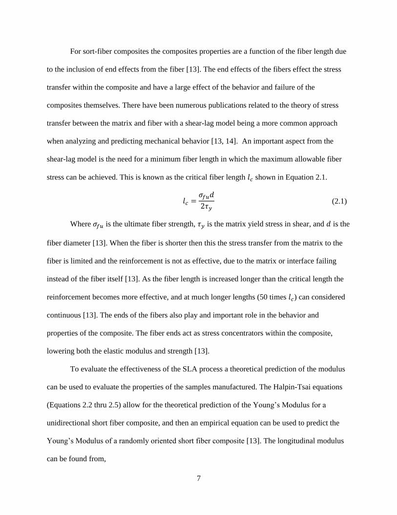
For sort-fiber composites the composites properties are a function of the fiber length due

to the inclusion of end effects from the fiber [13]. The end effects of the fibers effect the stress

transfer within the composite and have a large effect of the behavior and failure of the

composites themselves. There have been numerous publications related to the theory of stress

transfer between the matrix and fiber with a shear-lag model being a more common approach

when analyzing and predicting mechanical behavior [13, 14]. An important aspect from the

shear-lag model is the need for a minimum fiber length in which the maximum allowable fiber

stress can be achieved. This is known as the critical fiber length 𝑙𝑐 shown in Equation 2.1.

𝑙𝑐 =

𝜎𝑓𝑢𝑑

2𝜏𝑦 (2.1)

Where 𝜎𝑓𝑢 is the ultimate fiber strength, 𝜏𝑦 is the matrix yield stress in shear, and 𝑑 is the

fiber diameter [13]. When the fiber is shorter then this the stress transfer from the matrix to the

fiber is limited and the reinforcement is not as effective, due to the matrix or interface failing

instead of the fiber itself [13]. As the fiber length is increased longer than the critical length the

reinforcement becomes more effective, and at much longer lengths (50 times 𝑙𝑐) can considered

continuous [13]. The ends of the fibers also play and important role in the behavior and

properties of the composite. The fiber ends act as stress concentrators within the composite,

lowering both the elastic modulus and strength [13].

To evaluate the effectiveness of the SLA process a theoretical prediction of the modulus

can be used to evaluate the properties of the samples manufactured. The Halpin-Tsai equations

(Equations 2.2 thru 2.5) allow for the theoretical prediction of the Young’s Modulus for a

unidirectional short fiber composite, and then an empirical equation can be used to predict the

Young’s Modulus of a randomly oriented short fiber composite [13]. The longitudinal modulus

can be found from,

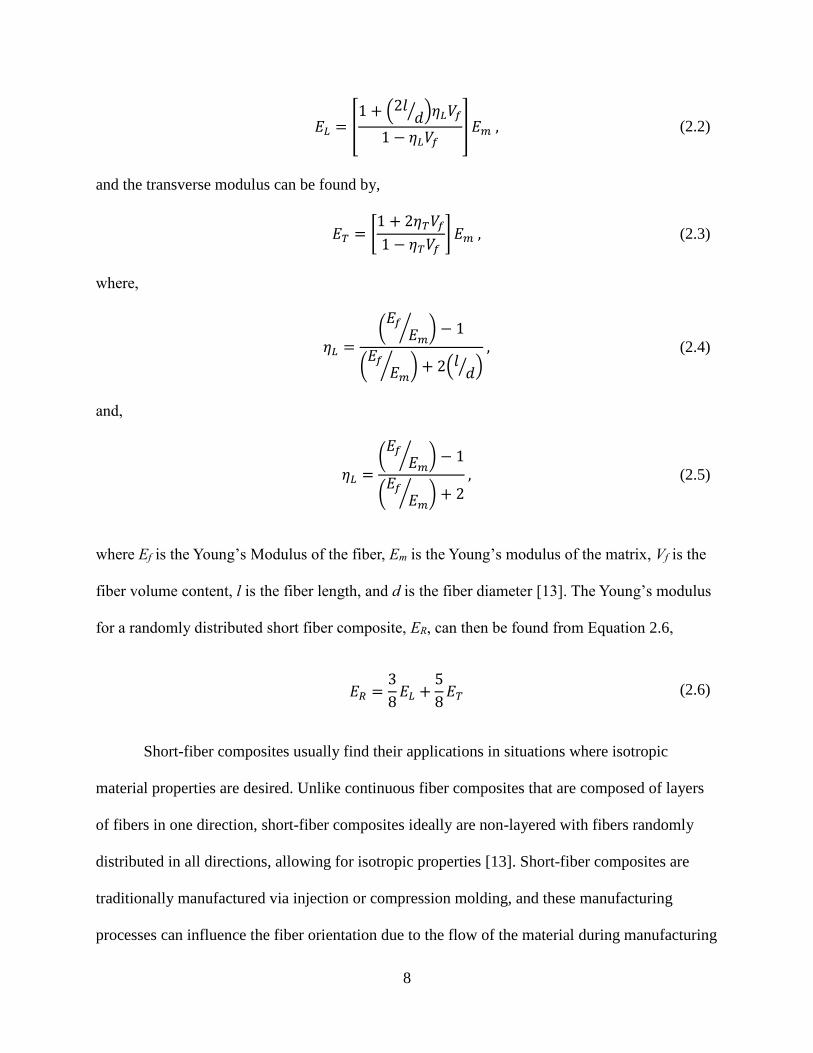
8

𝐸𝐿 = [1 + (2𝑙

𝑑⁄ )𝜂𝐿𝑉𝑓

1 − 𝜂𝐿𝑉𝑓] 𝐸𝑚 , (2.2)

and the transverse modulus can be found by,

𝐸𝑇 = [

1 + 2𝜂𝑇𝑉𝑓

1 − 𝜂𝑇𝑉𝑓] 𝐸𝑚 , (2.3)

where,

𝜂𝐿 =(

𝐸𝑓𝐸𝑚

⁄ ) − 1

(𝐸𝑓

𝐸𝑚⁄ ) + 2(𝑙

𝑑⁄ ) , (2.4)

and,

𝜂𝐿 =(

𝐸𝑓𝐸𝑚

⁄ ) − 1

(𝐸𝑓

𝐸𝑚⁄ ) + 2

, (2.5)

where Ef is the Young’s Modulus of the fiber, Em is the Young’s modulus of the matrix, Vf is the

fiber volume content, l is the fiber length, and d is the fiber diameter [13]. The Young’s modulus

for a randomly distributed short fiber composite, ER, can then be found from Equation 2.6,

𝐸𝑅 =3

8𝐸𝐿 +

5

8𝐸𝑇 (2.6)

Short-fiber composites usually find their applications in situations where isotropic

material properties are desired. Unlike continuous fiber composites that are composed of layers

of fibers in one direction, short-fiber composites ideally are non-layered with fibers randomly

distributed in all directions, allowing for isotropic properties [13]. Short-fiber composites are

traditionally manufactured via injection or compression molding, and these manufacturing

processes can influence the fiber orientation due to the flow of the material during manufacturing

9

final material properties [15]. While the flow induced alignment can be taken advantage of to

some extent, it can be limited due to the requirements of the mold design, and can be an

undesired effect when isotropic properties are desired [16]. To aid in design there have been

several analytical and experimental papers published in the area of fiber ordination and

distribution and their effects on the final material properties of parts produced using traditional

manufacturing methods [15-21].

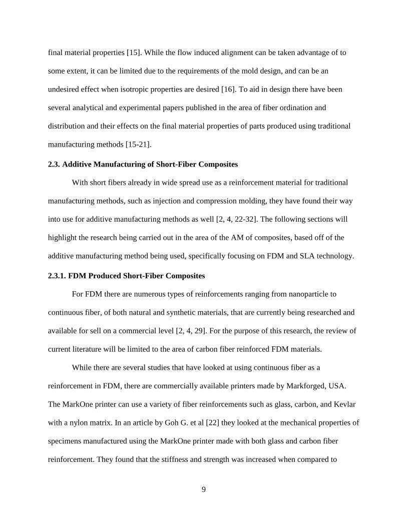
2.3. Additive Manufacturing of Short-Fiber Composites

With short fibers already in wide spread use as a reinforcement material for traditional

manufacturing methods, such as injection and compression molding, they have found their way

into use for additive manufacturing methods as well [2, 4, 22-32]. The following sections will

highlight the research being carried out in the area of the AM of composites, based off of the

additive manufacturing method being used, specifically focusing on FDM and SLA technology.

2.3.1. FDM Produced Short-Fiber Composites

For FDM there are numerous types of reinforcements ranging from nanoparticle to

continuous fiber, of both natural and synthetic materials, that are currently being researched and

available for sell on a commercial level [2, 4, 29]. For the purpose of this research, the review of

current literature will be limited to the area of carbon fiber reinforced FDM materials.

While there are several studies that have looked at using continuous fiber as a

reinforcement in FDM, there are commercially available printers made by Markforged, USA.

The MarkOne printer can use a variety of fiber reinforcements such as glass, carbon, and Kevlar

with a nylon matrix. In an article by Goh G. et al [22] they looked at the mechanical properties of

specimens manufactured using the MarkOne printer made with both glass and carbon fiber

reinforcement. They found that the stiffness and strength was increased when compared to

10

samples made of just nylon, but the properties where less than that of traditional composite

manufacturing methods [22]. The reason identified for this was the porosity of the extruded

material, voids with the layers, and weak bonding between the layers due to the lack of

consolidation within the manufacturing process [22].

A large amount of prior research and literature is available in the area of short carbon

fiber composites manufactured using FDM with a variety of matrix materials. In work by

Ferreira R. et al [23] they looked at using short carbon fiber as a reinforcement in a polylactic

acid (PLA) matrix. They compared a commercial available PLA printer filament with that of a

commercial available PLA filament with 15% weight carbon fiber. The study looked at the

effects of the print orientation on the material properties by holding the printing parameters the

same and varying the direction in which the test sample was printed. This samples were printed

with all layers in the same direction to best replicate a unidirectional laminate composite.

Ferreira R. et al found that the carbon fiber increased the stiffness the most (220%) in the

printing direction (longitudinal), while some improvement (160%) was seen in the transverse

stiffness [23]. They also observed a decrease in the tensile strength in all directions with this

being attributed to poor adhesion between the matrix and fiber [23]. It was also noted that the

printing process aligned the carbon fibers in the printing direction, and that voids were present in

the samples that where left behind by the printing process [23].

Work done by Ning F. et al [24] looked at the effects of different carbon fiber weight

percent on the material properties of composites parts made with an acrylonitrile butadiene

styrene (ABS) matrix. The samples were prepared using carbon fibers of 100 µm and 150 µm in

length at different fiber weights of 3, 5, 7.5, 10, and 15 percent, and both tensile and flexural

properties were investigated. The result suggested that the maximum improvements to tensile

11

strength, Young’s modulus, flexural strength, flexural modulus, and flexural toughness at a fiber

weight of 5% [24]. Above 5 wt.% the resulting mechanical properties began to decrease back to

or below that of the pure ABS samples, this being attributed to an increase in porosity within the

samples [24]. The authors found that as the carbon fiber amount was increased so did the number

void amount of the specimen, with the pores being generated due to gas evolution and physical

gap at the layer interfaces [24]. It was also found by Ning F. et al that increasing the fiber length

from 100 µm to 150 µm increased the tensile strength and Young’s modulus there was no

difference in the yield strength [24]. Ning F. et al study highlights one of the drawbacks of FDM,

being that the fabrication processes results in voids left in the sample in the form of gaps

between the layers and the individual extruded lines making up the layers themselves.

The work done by Tekinalp et al. [28] evaluated the material properties of carbon fiber

reinforced ABS, for fiber weights of 10, 20, 30, and 40 percent, and looked at the fiber

orientation effects of the FDM process. To accomplish this the Tekinalp et al. compared samples

prepare by both compression molding and FDM printing, and found that the FDM printing

process highly orientated the fibers in the printing direction [28]. While both samples had

increased tensile strength and Young’s modulus, due to the porosity in the FDM samples the

compression molded samples had overall higher properties [28]. While the fibers are orientated

in the direction of printing that direction is might not always be the direction of loading in a part

due to the different infill patterns available, and how the FDM process can vary depending on

what software is used. Tekinalp et al. point out, like others, that the porosity generated be the

FDM printing process has a negative effect on the material properties and is an issue that will

need to be addressed to further increase material properties [28].

12

From the literature, carbon fiber can offer a method of increasing the material properties

for FDM, but one of the main areas of concern that was pointed out was the formation of voids

and gaps due to the FDM printing process [23, 24, 28]. There is also the issue of the effect of the

printing processing parameters themselves. These include the nozzle temperature, bed

temperature, print speed, layer height, air gap, nozzle diameter, infill amount, infill pattern, and

number of perimeters to name a few. Changing few of these parameters can have an effect on

mechanical properties of the parts produced from the same material, as shown by Lanzotti A. et

al [33].

2.3.2. SLA Produced Composites

Whereas FDM based methods have a number of publications in the area of short fiber

composite characterization, the area of SLA manufactured composites is lacking in published

studies and available data using carbon fiber as a reinforcement. Because of this, the area of

review will be broadened to include other reinforcement materials and fiber types.

There have been various nanosized reinforcements studied as a method of increasing the

material properties of SLA manufactured parts such as: cellulose nanocrystals (CNC), multi-wall

carbon nanotubes (MWCNTs), and silver nanoparticles (AgNPs) [25-27, 31]. Feng X. et al [27]

used lignin-coated cellulose nanocrystals (L-CNC) at 0, 0.1, 0.5, and 1 weight percent with an

acrylic matrix. The research was carried out using Form+1 (Formlabs, Somerville, MA) which is

a bottom-up desktop SLA printer. At a loading of 0.5 wt.% L-CNC there was an increase in the

tensile strength and Young’s modulus by 3% and 5% respectively [27]. This was achieved only

after a thermal post-cure being carried out on the specimens with the non-post cured specimens

showing unimproved or reduced properties depending on the loading of L-CNC [27]. The

13

decrease in material properties that was seen at higher weight percent was attributed to poor

dispersion of the L-CNC and poor adhesion between the L-CNC and matrix [27].

Sandoval et al. [25] investigated a composite made from MWCNTs at 0.025 and 0.1

weight percent with an epoxy-based matrix using the commercial resin, DSM Somos®

WaterShed™ 11120. A top-down printer the 3D Systems SLA-250/50 machine (3D Systems,

Rock Hill, SC) was modified from a 47 liter vat to a 500 ml vat with the sweeping mechanism

removed, and a peristaltic pump was used to recirculate the resin mixture [25]. The research

looked at the increasing the tensile strength and fracture strength of the resin. For 0.025 wt.% of

MWCNTs, an increase in tensile strength of 5.7% with an increase in fracture strength of 26%

was reported. While at 0.10 wt.% an increase of 7.5% and 33% in tensile and fracture strength,

respectively was reported, but it was pointed out that at the higher loading of 0.1% MWCNTs

there were issues with agglomeration of the MWCNTs [25]. The elongation at break decreased

28% for the MWCNTs reinforced resin, and the fracture mode was reported as a brittle type

verse as more of a ductile failure mode that was seen in the pure resin [25].

Short glass fibers have been studied more as reinforcement materials for SLA in part due

to the decrease in opacity when compared to that of carbon fiber [4]. In one study, Cheah, C. et

al. [32] looked at using short glass fibers 1.6 mm in length at various fiber volume fractions of 0,

5, 10, 15, and 20 percent, and an urethane acrylic matrix, DeSolite SCR310. The experiment was

carried out for comparing molded and 3D printed samples. Although the paper does not state

what machine was used to print the samples it can be inferred that a top-down style was used

[32]. Cheah, C. et al saw improvements for all fiber volumes, with increased mechanical

properties achieved by increasing fiber amount and part shrinkage can be reduced. For a fiber

volume of 20% they were able to achieve an increase in tensile strength of 24%, and an 80%

14

increase in the Young’s modulus [32]. The top-down SLA machine that was employed resulted

in the manufacture of composites that were close to unidirectional in fiber orientation due to the

scraping step in between layers [32]. While the creation of unidirectional composites is desirable

in some applications, the leveling step would prevent the printing of an isotropic part, and

therefore could limit potential applications and restrict the printing process based on how the part

must be printed.

Along with short glass fibers, there have also be studies that have looked into the use of

continuous glass fiber as a reinforcement in SLA. Karalekas D. et al. [3] placed a single layer of

nonwoven glass fiber mats, of various thickness, within specimens produced using SLA. This

was done by pausing the printer at a predetermined build height placing the mat of the specimen

and resuming the print [3]. Karalekas D. et al. were able to show an increase in the Young’s

modulus, but a decrease in tensile strength for thinner mats. For the thicker mats the Young’s

modulus was shown to decrease, this was contributed to the inability for the photopolymer to

fully cure with in the thicker mats [3]. While this study was able to show that continuous glass

fibers could be placed into the part for reinforcement, the fact that it was added by hand during

the build process is inefficient, especially if multiple layers of fiber are to be used in the

manufacturing of a part, and would be difficult for the manufacturing of complex parts.

There is limited literature available on the use of carbon fibers with SLA, this could be

due in part to the limitation of carbon fibers being opaque [2, 4, 29]. Some research has been

carried out in this area using continuous carbon fiber by Gupta A. et al. [30] where to overcome

the issues of fully curing the part a dual curing system was used. The dual curing system

employed a photo initiator for initially curing the fiber and matrix in the desired geometry, and a

thermal initiator to cure the remaining resin. While Gupta A. et al was able to show that the

15

system was fully cured, they did not report any information on the material properties of the

composite produced [30].

2.4. Dual Cure Resin System

The use of a dual cure resin system, as proposed by Gupta A. et al [30], shows promise a

method of fully curing a short fiber composite manufactured using SLA, and this is demonstrated

in latter sections 5.1 and 5.2. The ability for the thermal initiator to cure the areas that the UV

light cannot, due to the opacity of the carbon fiber, could prove to be an effective method in the

manufacturing of short fiber composite via STL, shown in Figure 2.3.

Figure 2.3: Dual curing system.

16

3. OBJECTIVES

From the available literature in section 2.3, there is a limited amount of information and

results in the development of short-fiber composite manufactured using SLA, in particular ones

that use carbon fiber as the reinforcing material. The brittle nature of acrylic leads to a low

fracture toughness, and therefore, a low facture toughness in the parts made using SLA printing

[34, 35]. By incorporating fibers into the acrylic polymer, the fracture toughness could be

increased, along with other mechanical properties such as tensile strength and Young’s modulus

[13, 22, 32, 36, 37]. By taking advantage of the layer-by-layer manufacturing process it could be

possible to produce either an isotropic material, or an orthotropic material by influencing the

fiber orientation during the fabrication process by taking advantage of the differences in fiber

length verses layer height, as shown in Figure 3.1.

Figure 3.1: Effects of layer height on fiber orientation.

The purpose of this research will primarily be aimed at increasing the mechanical

properties of parts manufactured using SLA with fiber reinforcement. To accomplish this, the

research objectives are be defined as:

Determine and develop the processing parameters needed to manufacture short fiber

composite using SLA with carbon fiber as a reinforcement

Evaluate the effect of print orientation on material properties

Evaluate the effect of layer height on material properties

17

4. RESEARCH METHODOLOGY

This section will detail the materials and equipment used, the methods for sample

manufacturing, testing, and data analysis for this research. The section is organized into three

different main sub-sections, materials and equipment, sample manufacturing, and material

characterization. The materials and equipment section will look at the base materials and the

SLA printer used for this research. The section on sample manufacturing will cover the steps

used to produce the samples used in this study. While the material characterization section will

discuss the testing methods and data analysis used for characterization of the samples.

4.1. Materials and Equipment

The following subsections will detail the materials and SLA printer that were used to

produce both short-fiber composites, and the controls used in this study.

4.1.1. Moai Printer

A Moai Laser SLA Printer manufactured by Peopoly, and purchased from

MatterHackers, (Lake Forest, CA) as a DIY kit, was assembled and calibrated by the author. The

Moai is a bottom-up printer that uses a 405 nm 70-micron spot size laser and is based on an open

sourced design. This allows for the modification of both hardware and software along with direct

G-Code modification, with the limitation of the firmware being closed source. All printing

settings used in the research are in reference to the Moai printer using firmware version 1.6.

Figure 4.1 is of the Moai printer currently being used to conduct this study.

18

Figure 4.1: Moai SLA printer.

4.1.2. Photopolymer Resins

The photopolymer resin being used in this research is Moai Standard Clear resin, by

Peopoly. It is an acrylic-based photopolymer designed to work with the Moai printer being used

in this research. The data in Table 4.1 shows the given makeup of the resin according to the

manufacture.

Table 4.1: Peopoly resin constituents [9].

Chemical Approximant Weight (%)

Urethane Acrylate 30-50

Acrylic Monomer 55-60

1,6 - Hexanediol Diacrylate 5-15

Photo initiator 0-5

4.1.3. Carbon Fiber

Carbon fiber has been used as a reinforcement in polymer matrix composite for many

years [38]. This material is widely used for its high strength, modulus, and thermal resistance

19

along with its light weight. The high specific properties lead to carbon fiber composites being

used in a number of industries such as, aerospace, automotive, sports, aeronautics, and leisure

[39, 40]. The exact mechanical properties of carbon fiber can vary depending on the precursors

used and the processing parameters during its manufacturing. Table 4.2 shows the mechanical

properties of some carbon fibers depending on what precursors are used in their manufacturing

[41].

Table 4.2: Mechanical properties of various carbon fiber [41].

Precursor Tensile Strength (GPa) Tensile Modulus (GPa)

Polyacrylonitrile (PAN) 2.5-7.0 250-400

Mesophase Pitch 1.5-3.5 200-800

Rayon 1.0 50

The primary carbon fiber that will be used in this study will be, Toray T-700. The fiber

was purchased form Composite Envisions (Wausau, WI) as a chopped 3 mm fiber and is sized

for epoxies. The fiber was then milled in a Retsch Rotor Beater Mill SR 300 (Retsch GmbH,

Haan, Germany) using a 120 µm screen. The milled fiber was then sieved using a stack of

screens, with a stacking sequence of 2 mm, 250 µm, 106 µm, and 76 µm. The fibers were

collected in-between the 106 µm and 76 µm screens.

To evaluate the size of the milled carbon fiber produce, a glass slide was prepared that

was coated with a thin layer of the Moai resin. A sample of fibers was then applied on the

surface of the glass slide, and held in front of the light in the UV cure oven for 1 minute. A

sample of fibers were observed using an Axovert 40Mat (Carl Zeiss AG, Oberkochen,

Germany), with images obtained by a ProgRes C10plus camera (Jenoptik AG, Jena, Germany),

to determine the average length along with the length distribution. The processed fibers were

then placed in an oven at 80 °C and dried for a minimum of 8 hours before use. The mechanical

properties of the fibers as provided by the manufacturer are shown in Table 4.3.

20

Table 4.3: Toray T-700 fiber properties [42].

T-700 Fiber Properties

Fiber Diameter 7 µm

Fiber Length 3 mm

Tensile Strength 4.90 GPa

Tensile Modulus 230 GPa

A second fiber was also used during this research, Carbiso MF SM45R-100

manufactured by ELG Carbon Fibre Ltd, (Conseley, UK). The fibers are reclaimed from end-of-

life composite materials that are then take through a modified pyrolysis process, milled, and

sorted [43]. The fibers that were used were dried for a minimum of 8 hours in an oven at 80°C.

Due to the reclamation process the fiber is unsized, and has the mechanical properties, as

provided by the manufacturer, shown in Table 4.4.

Table 4.4: Carbiso MF SM45R-100 fiber properties [43].

Carbiso MF Fiber Properties

Fiber Diameter 7 µm

Fiber Length 80-100 µm

Tensile Strength 4.150 GPa

Tensile Modulus 230-255 GPa

4.1.4. Thermal Initiators

The exact make up and composition of the base resin being used is not known, therefore

a variety of thermal initiators will be investigated in order to identify the optimum thermal

initiator to be used in a dual cure system. This will be based off of the thermal initiators

solubility with the resin system, the stability of the resin system at room temperature, and the

temperatures needed for post-curing of the samples. The initial thermal initiators to be

investigated are summarized in Table 4.5.

21

Table 4.5 Thermal initiators to be investigated for a dual cure resin system.

Name Trade Name CAS Number Source

Dilauroyl Peroxide Luperox LP 105-74-8 Alfa Aesar

Cumene Hydroperoxide -- 80-15-9 Sigma-Aldrich

Dicumyl Peroxide -- 80-43-3 Sigma-Aldrich

Tert-Butyl Peroxybenzoate Luperox P 614-45-9 Sigma-Aldrich

Benzoyl Peroxide Luperox A98 94-36-0 Alfa Aesar

4.2. Sample Manufacturing

The following subsections will detail the processing parameters that will be used to

produce both short-fiber composites, and the controls that will be used in this study.

4.2.1. Resin Manufacturing

To ensure that the fiber and any other added components are well dispersed the following

process was carried out:

1. The necessary fiber amount is added to the resin and hand mixed for 2 minutes.

2. The resin mixture is then mixed using a high-speed mixer for 20 minutes.

3. The resin mixture is then placed in an ice bath and sonicated in 10 second pluses, with a 1

minute break between pulses, for a total of 5 minutes of sonication.

4. The necessary thermal initiator amount is then added.

5. The resin mixture is then mixed in a high-speed mixer for 20 minutes.

6. The resin mixture is then degassed in a vacuum chamber for 10 minutes, or until bubbling

stops.

The resin and fiber was first mixed and sonicated separately, due to the increase in

temperature of the resin during this process, as a way of protecting the thermal initiator. The

vacuum chamber is used to remove any air trapped within the system that could then cause voids

within the manufactured sample. Upon the completion of the degassing the resin is immediately

used to manufacture samples to limit the time allowed for setting of the fiber to occur.

22

4.2.2. Processing Parameters for 3D Printing Parts

To create samples for testing, the test samples were designed first using SolidWorks

(Dassault Group, Paris, France), a CAD software, to create the need geometry of the specimens.

The files were then exported from Solidworks in a Standard Tessellation Language (stl) file

format. The stl files are then loaded into another software package, XYZware (New Kinpo

Group, New Taipei City, Taiwan) that is used to orient the part in the desired print orientation,

and used to generate the necessary supports to facilitate the printing process. XYZware was used

to generate all supports and part orientations for this research. The supports that are made within

XYZware serve multiple purposes such as elevating the part above and securing it to the print

bed. The silicon layer that is coated along the bottom of the vat is deformed when the bed is

initially lowered. The part to be printed is raised up from the print bed by these supports a

sufficient distance, generally 3 to 6 mm, to allow for compensation due to the compression of the

silicon layer so as to not affect the geometry of the part being printed.

Generally, when printing with bottom-up style machines the part is oriented to reduce the

size of the cross-section of the largest axis of the part. This is done to reduce the stresses within

the part when the peel step is carried out. If too high of stresses are present it can result in layer

separation, warping of the part, or separation/shifting from the printing bed. To be able to print

the parts need for this research it was necessary to the increase the amount and size of some of

the supports used. An example of the supports applied in the XYZware software is shown in

Figure 4.2.

23

Figure 4.2: Before (left) and after (right) support material being added.

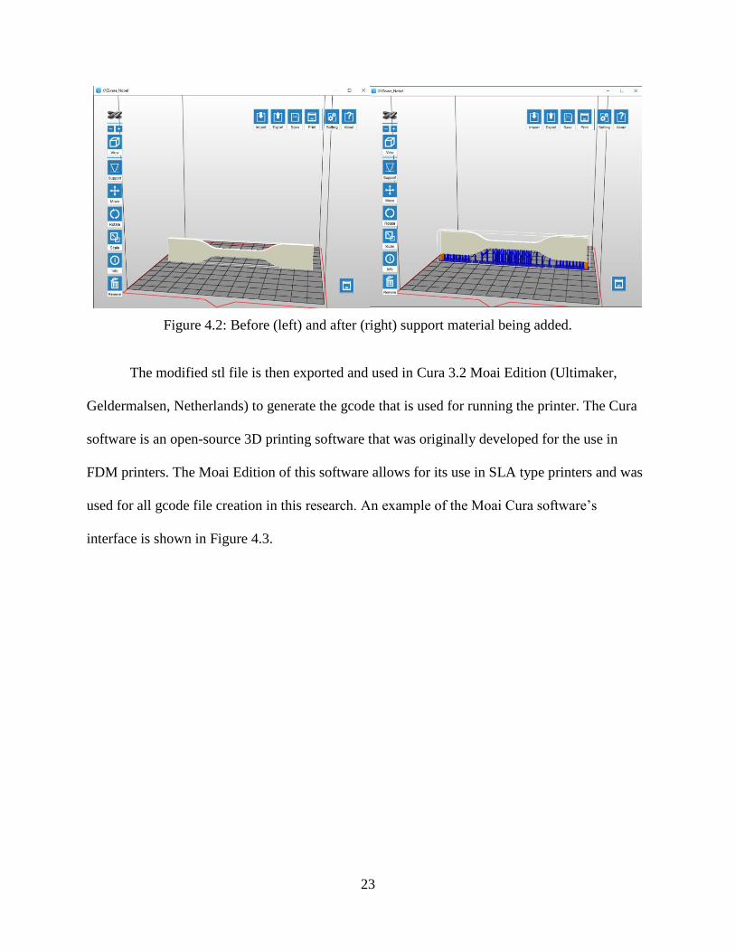
The modified stl file is then exported and used in Cura 3.2 Moai Edition (Ultimaker,

Geldermalsen, Netherlands) to generate the gcode that is used for running the printer. The Cura

software is an open-source 3D printing software that was originally developed for the use in

FDM printers. The Moai Edition of this software allows for its use in SLA type printers and was

used for all gcode file creation in this research. An example of the Moai Cura software’s

interface is shown in Figure 4.3.

24

Figure 4.3: Cura slicing software.

Within the Cura software is where the modifications to the printing parameters can be

made. The most important of these would be the layer height, laser speed, and infill amount. For

samples printed with neat (non-fiber reinforced) resin, the layer height would have the most

effect on the print resolution when trying to print fine/small details. For the application in

printing short-fiber composites it is proposed that the layer height can be used to influence the

fiber orientation.

The laser speed, along with the laser power which is set directly on the printer, controls

the amount of energy being delivered to the area, and therefore directly effects the curing of the

part being printed [5]. The infill amount is used to control the amount of space between the laser

scans within the part, if any that occurs during the printing process. The infill patterns can also

be change, but only the line pattern was used for this research. While the laser spot is where the

energy is being delivered to initiate the polymerization, there is an area around the laser spot that

25

the polymerization process spreads past [5]. This allows for the spacing between the scan lines,

but stills allows for curing of part into a solid. By increasing the space between the scans the

print time can be reduced, but if the spacing is increased too much the part can fail to fully cure

and as a result a solid part will not be formed.

For all samples that are manufactured using the 3D printer for this research a naming

convention will be implemented that will reference the long axis of the sample to the printed

layer orientation, this is illustrated in Figure 4.4.

Figure 4.4: Sample long axis orientation.

4.2.3. Post-Processing of 3D Printed Parts

For all samples prepared, the finished parts were washed in ethanol after being removed

from the build platform. This allows for the removal of any uncured resin, and in the case of the

fiber reinforced samples any lose fibers from the surface. The supports that were generated

during the printing process are left in place at this time to support the sample while it was being

post-cured.

For the neat (non-fiber reinforced) samples, the resin manufacturer recommends post-

curing in a 405 nm UV light for a period of time until the surface cannot be scratched by a finger

26

nail [9]. While other resin manufactures provide more detailed post-curing instructions of

elevated temperature and times. For this research the neat samples were post-cured in an in-

house built cure oven, shown in Figure 4.5.

Figure 4.5: UV cure oven.

This oven consist of three 25 Watt LED UV lights, a heating element, and a rotating

platform. The temperature and the time for the post-cure can be adjusted by the use of PID

controller. For the neat samples a temperature of 80 °C was used while being exposed to the UV

light for 1 hour.

Unless otherwise stated the fiber reinforced sample’s post-curing was carried out using a

VWR Forced Convection Oven (VWR International, Radnor, PA), shown in Figure 4.6.

27

Figure 4.6: Post-curing oven.

The temperature that the samples are post-cured at will be dependent on the thermal

initiator that is used, with DSC being used to determine at what temperature the resin system will

begin to initiate, and how long the samples will need to be held at that temperature.

After post-curing is complete, the supports are removed from the sample. This leaves

behind dimples in the surface that can act as defects that affect the ultimate tensile strength of the

material during testing [44]. An example of these surface defects are shown in Figure 4.7.

Figure 4.7: Surface defects from support removal.

28

To completely remove the dimples, the area that had the supports attached were sanded

with increasingly finer grits of sand paper, ranging from 60 to 600, with care taken to preserve

the sample geometry which varies depending on the desired testing. This was done for all printed

samples used in this study. Figure 4.8 shows the progression at various points in removing the

support material and surface defects.

Figure 4.8: Removal of supports and surface effects. A) Supports removed, B) sanded with 60

grit paper, and C) sanded with 600 grit paper

4.3. Material Property Characterization of 3D Printed Composites

The following subsections will detail the material characterization that was used to

experimentally evaluate both short-fiber composites and the controls that were used in this study.

4.3.1. Thermal Initiator Selection

In an effort to identify a thermal initiator that worked best as a dual cure system, several

were evaluated with the first key issue being the solubility of the initiator within the resin. As

mentioned in section 2.3.2, Gupta A. et al [30] proposed a dual cure system using Luperox LP

that remained in a solid state in the sample until post-curing at an elevated temperature. To

achieve a good dispersion of the initiator within the system different thermal initiators were

mixed at a loading of 1 wt.% with the resin. The mixtures were monitored to determine if the

29

initiator was soluble in the resin, and also monitored for one week at room temperature to insure

stability for the 3D printing process.

Upon completion of solubility testing the selected thermal initiators were evaluated

experimentally via differential scanning calorimetry (DSC) in accordance with ASTM E2160

[45]. The testing was carried out over a range from 25°C to 180°C at a ramp rate of 10°C/min,

using a Q20 DSC (TA Instruments, New Castle, DE). This was done to determine the thermal

initiators onset temperature, and to experimentally determine if any reactions are occurring after

UV curing. The samples were tested at a fiber volume (Vf) of 5%, and a thermal initiator content

of 1 wt.% of thermal initiator to 99 wt.% of Moai resin. The neat Moai resin was also tested to

determine if there is any activation of the photo initiator at elevated temperatures.

For each sample tested two runs were carried out. The first was of an uncured sample,

and the second was a sample that had been UV cured by placing the DSC pan in the UV cure

oven 25.4 mm away from the light source for one minute at room temperature. All graphs

produced from the DSC data were made using TA Universal Analysis (TA Instruments, New

Castle, DE).

4.3.2. Viscosity Testing

To examine both the effects of the fiber reinforcement and thermal initiator on the resin

system, viscosity testing was carried out using a AR-G2 Rheometer (TA Instruments, New

Castle, DE) with a 40 mm steel parallel plate and Peltier plate, shown in Figure 4.9.

30

Figure 4.9: AR-G2 rheometer.

The gap between the plates was set to 1000 μm to allow for at least 10 times the length of

the fiber (assumed a fiber length of 100 μm) in the resin, as per the AR-G2 TA Instruments

rheology manual [46]. Two controlled shear rate test were ran for each sample, one from a range

of 1 to 25 s-1 on a linear scale with 25 sample points, and the other from 1 to 100 s-1 on a log

scale at 5 decades. All test were carried out at room temperature, and the data was post processed

using Rheology Advantage Data Analysis (TA Instruments, New Castle, DE).

The experimental data points where then fitted with a model that resulted in the smallest

standard error. This was found to be Ostwald-de-Waele equation (power law equation) for both

of the testing rates, shown in Equation 4.1,

𝜏 = �̅��̇�𝑛, (4.1)

31

were, τ is the shear stress, �̇� is the shear rate, n is the power-law index, and �̅� is the consistency

index of the polymer [47]. The best fit was determined based off of the standard error of model

with the smaller number being the best fit and defined as Equation 4.2,

𝑆𝐸 =

[∑(𝑥𝑚 − 𝑥𝑐)2

𝑛 − 2 ]1/2

𝑅𝑎𝑛𝑔𝑒𝑥1000,

(4.2)

where Xm is the measured value, XC is the calculated value of x for each data point, n is the

number of data points, and the range is the maximum value of Xm [46, 47].

4.3.3. Tensile Testing

4.3.3.1. Sample Manufacturing and Testing

The tensile testing was carried out using an Instron 5567 load frame (Instron, Norwood,

MA), a 25.4 mm extensometer, and a 2 kN load cell. The load frame was controlled and data

collected using Bluehill software (Instron, Norwood, MA). While there are no ASTMs directly

concerning 3D printed materials, all tensile testing will be carried out referencing ASTM D638

[48] and ASTM 3039 [49]. The specimen geometry was of the type IV according to ASTM

D638, with the specimen dimensions shown in Figure 4.10 [48].

Figure 4.10: Tensile testing specimen (all dimensions in mm).

The type IV specimen was chosen due to the limiting size of the build plate (130 mm x

130 mm) of the Moai printer being used to conduct this research. All samples were tested at a

32

constant cross-head rate of 1 mm/min, so failure of the specimen occurred within 1 to 10 minutes

of testing, per ASTM D3039 [49]. For each sample 5 specimens were tested.

To evaluate the effect of using SLA to manufacture short-fiber composites the sample

parameters that were evaluated are; carbon fiber reinforcement, thermal initiator effects, different

layer heights, and different print orientations. So as to determine what effect the different

manufacturing parameters and fiber volumes have on the Young’s modulus and ultimate tensile

strength. To develop the experiment a two level full factorial design was used with the above

mentioned parameters. Table 4.6 shows the identification of each factor, while Table 4.7 is the

experimental test matrix.

Table 4.6: Tensile testing experimental variables.

Factor Level 1 Level 2

Print Orientation 0° 90°

Layer Height 100 µm 50 µm

Fiber Volume 0 5% Vf

Thermal Initiator 0 0.5 wt%

33

Table 4.7: Tensile testing test matrix.

Test Number Print Orientation Layer Height Fiber Volume Thermal

Initiator

1 1 1 1 1

2 1 1 1 2

3 1 1 2 1

4 1 1 2 2

5 1 2 1 1

6 1 2 1 2

7 1 2 2 1

8 1 2 2 2

9 2 1 1 1

10 2 1 1 2

11 2 1 2 1

12 2 1 2 2

13 2 2 1 1

14 2 2 1 2

15 2 2 2 1

16 2 2 2 2

4.3.3.2. Data Analysis

The experimental data was evaluated statistically to identify any trends using MatLab

R2016b (MathWorks, Natick, MA), and Excel (Microsoft, Redmond, WA). The effects of layer

high and print orientation were compared using a one-way ANOVA analyst at a 95% confidence

interval. While ANOVA allows for the identification if there is a difference between the means

within a group it will not identify which groups are different [50]. To identify which samples

differ from each other additional statistical analysis was carried out. Tukey’s Honest Significant

Difference (HSD) was chosen to identify which samples differ from each other within the groups

compared using ANOVA. The Tukey HSD is calculated by first applying Equation 4.3.

𝑄𝐻𝑆𝐷 =

𝑀𝑖 − 𝑀𝑗

√𝑀𝑆𝑊

𝑛

, (4.3)

where Mi and Mj are the means of the pairs to be compared, with Mi being larger then Mj, MSW is

the mean square within from the ANOVA analysis, and n is the sample size [50-52]. The QHSD

34

value is then compared to a Qcritical value based off of sample size, degrees of freedom for the

error term, and desired confidence level, and can be found from numerous sources as published

tables [50, 51].

The Tukey test for the tension samples was carried out at both a 95% and 99%

confidence level with the highest confidence level being reported per compared pair, with the

corresponding Qcritical values shown in Table 4.8 [51].

Table 4.8: Qcritical for Tukey HSD tension testing.

Confidence Level Qcritical

95% 4.3729

99% 5.3738

4.3.4. Flexural Testing


The flexural testing was carried out using an Instron 5567 load frame (Instron, Norwood,

MA) with a 2 kN load cell. The load frame was controlled and data collected using Bluehill

software (Instron, Norwood, MA). While there are no ASTMs directly concerning 3D printed

materials, all flexural testing will be carried out referencing ASTM D790 [53]. The flexural

testing was carried out as a three-point bending utilizing center loading, with specimens having a

span-to-thickness ratio of 16:1. The crosshead rate for testing was determine using Equation 4.4,

as per ASTM D790.

𝑅 =

𝑍𝐿2

6𝑑 (4.4)

where R is the crosshead rate, Z is the rate of straining of the outer fiber (0.01), L is the support

span, d is the depth of the beam [53]. The specimen geometry was determined based off of

ASTM D790 so as to fit within the build envelope of the printer, with the specimen dimensions

shown in Figure 4.10 [53].

35

Figure 4.11: Flexural testing specimen (all dimensions in mm).

To evaluate the effect of using SLA to manufacture short-fiber composites samples were

tested at, different fiber volumes, different layer heights, and print orientations so as to determine

what effect the different manufacturing parameters and fiber volumes had on the flexural

strength and stiffness. To develop the experiment a two level full factorial design was used with

the above mentioned parameters. Table 4.9 shows the identification of each factor, while Table

4.10 is the experimental test matrix.

Table 4.9: Flexural testing experimental variables.






36

Table 4.10: Flexural testing test matrix.


Initiator

1 1 1 1 1

2 1 1 1 2

3 1 1 2 1

4 1 1 2 2

5 1 2 1 1

6 1 2 1 2

7 1 2 2 1

8 1 2 2 2

9 2 1 1 1

10 2 1 1 2

11 2 1 2 1

12 2 1 2 2

13 2 2 1 1

14 2 2 1 2

15 2 2 2 1

16 2 2 2 2


The data analysis for the flexural testing was carried out in the same manner as the tensile

testing, as described in section 4.3.3.2. The same parameters for the Qcritical that were used for the

tensile testing were used for the flexural testing due to the same sample size.

4.3.5. Fracture Toughness Testing


The fracture toughness testing was carried out using an Instron 5567 load frame (Instron,

Norwood, MA) with a 2 kN load cell. The load frame was controlled and data collected using

Bluehill software (Instron, Norwood, MA). While there are no ASTMs directly concerning 3D

printed materials, all fracture toughness testing was carried out referencing ASTM D5045 [54].

The testing was conducted using the three point bend method that utilizes a single edge notched

beam (SENB) specimen [54]. To find the necessary specimen geometry ASTM E399 [55] was

referenced to find the minimum recommended thickness based off the ratio of yield strength to

37

Young’s modulus. Based off of ASTM D5045 and the printer bed size a thickness, B, was

chosen as 7 mm. The other dimensions of the specimen are then based off of this value to insure

plane-strain conditions and are shown in Figure 4.12 [54].

Figure 4.12: SENB specimen for fracture testing (all dimensions in mm).

As per ASTM D5045, a natural crack was generated by sliding a razor blade in the 3D

printed notch until the crack was of the specified length [54]. The fracture toughness was then

calculated per section A1.4 of ASTM D5045 [54].

To evaluate the effect of using SLA to manufacture short-fiber composites samples were

tested at different fiber volumes, different layer heights, and print orientations so as to determine

what effect the different manufacturing parameters and fiber volumes had on the fracture

toughness. To develop the experiment a two level full factorial design was used with the above

mentioned parameters Table 4.11 shows the identification of each factor, while Table 4.12 is the

experimental test matrix.

Table 4.11: Fracture toughness testing experimental variables.






38

Table 4.12: Fracture toughness testing test matrix.


Initiator

1 1 1 1 1

2 1 1 1 2

3 1 1 2 1

4 1 1 2 2

5 1 2 1 1

6 1 2 1 2

7 1 2 2 1

8 1 2 2 2

9 2 1 1 1

10 2 1 1 2

11 2 1 2 1

12 2 1 2 2

13 2 2 1 1

14 2 2 1 2

15 2 2 2 1

16 2 2 2 2


The data analysis for the flexural testing was carried out in the same manner as the tensile

testing, as described in section 4.3.3.2. With Qcritical values due to the different sample size shown

in Table 4.13 [51].

Table 4.13: Qcritical for Tukey HSD fracture toughness testing.

Confidence Level Qcritical

95% 4.7511

99% 6.1023

4.3.6. Fiber Volume Consistency

To evaluate the consistency of the fiber volume content, due to the various printing times

need in manufacturing samples, burn off testing was carried out. The samples that were analyzed

were taken at 3 different points from flexural specimens printed in the 90° print orientation as 2

mm sections, as shown in Figure 4.13.

39

Figure 4.13: Burn off sample testing areas.

The testing was carried out using a Thermolyne Type 2000 muffle furnace (Thermolyne,

Dubuque, IA), pictured in Figure 4.14.

40

Figure 4.14: Thermolyne muffle furnace.

The burn off testing was carried out referencing ASTM D3171-15 procedure G, with the

samples being held at a temperature of 550 ºC for 1 hour [56]. Two specimens each were tested

for the two different layer heights to determine at what point, if any, the print times start to effect

the fiber content due to settling. The print times for the 100 μm and 50 μm layer heights were

3.00 and 5.25 hours, respectively.

4.3.7. Composite Void Content

To determine the void content of the carbon fiber composites, first the density was found

as per ASTM D792-13 Test Method A [57]. Cubes were printed of 0.5 wt.% Luperox P at 100

μm layer height, and for 100 μm and 50 μm layer height for resin containing 5% Vf carbon fiber

and 0.5%wt Luperox P. All samples were prepared and post-cured as outlined in section 4.2. The

specimen geometry used is shown in Figure 4.15.

41

Figure 4.15: Void content and density test specimen (all dimensions mm).

The water temperature at the time of testing was 23.7 ºC, and the density was found per

section 13.1 and 13.2 of ASTM D792-13 [57]. Two specimens were tested per sample and the

same composite samples that were used to find the density were then used to determine the void

content as per ASTM D3171-15 Procedure G [56]. The burn off testing was carried out using the

same Thermolyne Type 2000 muffle furnace that was used in section 4.3.6. Two specimens per

sample were tested with a burn off time of 1.5 hours at 550 ºC.

4.3.8. Post-Cure Shrinkage

To determine the shrinkage that occurred during the post-curing process samples were

prepared of the same geometry used for the density measurements, shown in Figure 4.15. For the

testing 5 specimens per sample were prepared and evaluated. The samples that were tested are

shown in Table 4.14.

Table 4.14: Post-cure shrinkage test samples.

Sample Constituents Layer Height

Moai Resin 100

Moai Resin 50

Moai Resin + 0.5 wt.% Luperox P 100

Moai Resin + 0.5 wt.% Luperox P 50

Moai Resin + 0.5 wt.% Luperox P + 5% Vf Carbon Fiber 100

Moai Resin + 0.5 wt.% Luperox P + 5% Vf Carbon Fiber 50

42

The samples were prepared as per sections 4.2.1 and 4.2.2, and the cubes numbered for

easy identification. The sides of the cubes were marked with an X, Y, and Z in reference to the

printing axis defined by the Moai printer. The sides were measured using a digital caliper before

post-curing. The samples were then post-cured as per section 4.2.3, and measured again. The

difference in the corresponding sides and the overall volume difference was then calculated

along with the mean and standard deviation.

4.3.9. Scanning Electron Microscopy

Scanning electron microscopy (SEM) will be utilized to examine the fracture surface of

tested samples. This will allow for examination of the fracture surface in determining failure

types, and to evaluate the dispersion and the orientation of the fibers with in the sample [58].

Samples were attached to cylindrical aluminum mounts with colloidal silver paste (SPI Supplies,

West Chester, Pennsylvania, USA). The specimens were sputter coated (Cressington 108auto,

Ted Pella, Redding, California, USA) with a conductive layer of gold. Images were obtained

with a JEOL JSM-6490LV scanning electron microscope (JEOL USA, Inc., Peabody MA,

USA); energy-dispersive X-ray information was collected at an accelerating voltage of 15 kV

using a Thermo Scientific UltraDry Premium silicon drift detector with NORVAR light element

window and Noran System Six imaging system (ThermoFisher Scientific, Madison WI, USA).

43

5. RESULTS AND DISCUSSION

5.1. UV Cured Short Fiber Reinforced Composites

To evaluate the effectiveness as carbon fiber as a reinforcement in SLA printed parts it

was first attempted to print parts using only the photo initiator that was present in the Moai resin.

The following section 5.1.1 summarizes the results from evaluating the tensile properties of these

parts.

5.1.1. Tensile Testing

A short-fiber composite resin consisting of Carbiso MF SM45R-100 carbon fiber and

Moai resin, at a fiber volume of 5%, was prepared as detailed in section 4.2.1 with the exception

of the addition of a thermal initiator. Tensile samples were prepared as per sections 4.2.2 and

4.2.3 with a layer height of 50 μm and 100 µm and a print orientation of 0º. Due to no thermal

initiator being used, the samples were post-cured in the same manner as the neat samples in the

UV oven in section 4.2.3. The tensile testing was carried out as described in section 4.3.3.

Representative stress-strain curves of the neat Moai resin and 5% Vf for 100 μm and 50 µm layer

heights are shown in Figure 5.1 for comparison.

44

Figure 5.1: Representative stress-strain curves.

The maximum tensile strength and Young’s modulus was found as specified in ASTM

D638 section 11.2 and 11.4 respectively with the results summarized in Table 5.1.

Table 5.1: Tensile testing results for UV cured at 5% Vf carbon fiber.

Fiber

Volume (%)

Print

Orientation

Layer Height

(µm)

Tensile Strength

(MPa)

Young’s Modulus

(GPa)

0 0° 100 58.9 ± 5 2.72 ± 0.059

5 0° 100 26.2 ± 4.1 1.98 ± 0.03

5 0° 50 52.0 ± 2.3 2.64 ± 0.04

From the results in Table 5.1, the addition of the carbon fiber did not increase any of the

material properties when compared to the neat Moai resin properties. Applying the Halpin-Tsai

Equations (Equations 2.2 thru 2.5) to predict the Young’s modulus for a randomly distributed

short fiber composite, ER, (Equation 2.6) the theoretical modulus should be 4.27 GPa.

45

For the sample printed at 100 µm layer height there is a decrease in both strength and

modulus, while the sample printed at 50 μm layer height shows a smaller decrease. This is due to

the UV radiation being unable to activate the photo initiator in order to fully cure the resin due to

the opaque nature of the carbon fiber [2, 4, 29, 30]. The increase of properties between the 100

μm and 50 µm layers could be due to the fibers being aligned in the direction of the tensile

testing, but is more likely due to the decreased layer height allowing for more of the matrix to be

cured. This is evident by the fact that the material properties of the sample are approaching that

of the neat resin. To counter act this the use of a dual cure resin system is implemented for the

remainder of this research.

5.2. Dual Cured Short Fiber Reinforced Composite

5.2.1. Thermal Initiator Evaluation

5.2.1.1. Solubility and Stability of Thermal Initiators

In order to fully cure all of the resin with in the sample the use of a dual cure system that

uses both a photo initiator and a thermal initiator was investigated. The first thermal initiator

investigated was Luperox LP. This was chosen because of its use by Gupta A. et al [30] in a dual

cure system, as mentioned in section 2.3.2. One issue that had arisen in Gupta A. et al. work and

the current work is that Luperox LP is a solid at room temperature and would not completely

dissolve in the base resin being used [30].

To attempt to overcome the solubility issues of the Luperox LP it was first dissolved in

toluene, which was then mixed into the base resin. This addition of solvent to the resin lead to a

large decrease in viscosity causing the carbon fibers to settle out of the resin quickly. To remove

the toluene from the resin a vacuum chamber was used to evaporate the toluene and remove it

from the resin. To verify that the toluene was removed from the resin, the weight of the resin and

46

thermal initiator being added was recorded along with the weight of the toluene being added. The

mixture was then kept under vacuum, and the weight checked until the weight of the toluene was

removed from the mixture. The other thermal initiators that were investigated, shown in Table

4.5, were either liquid or would dissolve into the Moai resin on their own, and needed no

additional steps to incorporate into the system.

The solubility and stability of the thermal initiators were tested as outlined in section

4.3.1 with a 1 wt.% of thermal initiator to 99 wt.% of the Moai resin. The results of the solubility

and stability testing are summarized in Table 5.2.

Table 5.2: Thermal initiator solubility and stability testing.

Thermal Initiator Solubility Stability

Luperox LP Yes, with additional steps Yes

Luperox P Yes Yes

Dicumyl Peroxide Yes Yes

Cumene Hydroperoxide Yes Yes

Luperox A98 Yes No, gelled after 24 hours

Due to Luperox A98 gelling the system within 24 hours of mixing it was removed for

consideration as a suitable thermal initiator.

5.2.1.2. DSC

The DSC testing was carried out as outlined in section 4.3.1 for the Moai resin and all

thermal initiators but Luperox A98 and Luperox LP. The Luperox A98 was removed from the

study due to gelling, and the onset temperature for the Luperox LP (93.35 °C) was available

from Gupta A. et al paper [30]. The results of the DSC testing are shown in Appendix A, Figure

A.1 thru Figure A.4, and are summarized below in Table 5.3.

47

Table 5.3: Thermal initiator onset temperature from DSC curves.

Thermal Initiator Onset Temperature (°C) 10 Hour Half-life (ºC) [59]

Luperox P 115.99 104

Dicumyl Peroxide 116.83 114

Cumene Hydroperoxide 104.01 135

Based off of the results from the thermal initiator testing Luperox P was chosen as the

first thermal initiator to be evaluated for the dual cure resin system. Luperox is a liquid at room

temperature therefore it does not require additional processes to incorporate into the resin.

5.2.1.3. Resin Viscosity

To determine the effect of the incorporation of the different constituents on the viscosity

of the resin it was evaluated as outlined in section 4.3.2., and tested at a room temperature of

24.5 ºC. The samples that were tested and their viscosities are shown in Table 5.4.

Table 5.4: Viscosity of composite resins.

Sample Viscosity (Pa s)

Moai Resin 0.517

Moai Resin + 0.5% wt. Luperox P 0.497

Moai Resin + 5% Vf Carbon Fiber 0.815

Moai Resin + 5% Vf Carbon Fiber + 0.5% wt. Luperox P 0.649

With representative graphs for the testing done for a shear rate of 1 s-1 to 25 s-1 in Figure

5.2 , and for rates of 1 s-1 to 100 s-1 Figure 5.3, with the individual graphs with fitted curves in

APPENDIX A, Figure A.5 thru Figure A.12.

48

Figure 5.2: Viscosity testing with for shear rate from 1 s-1 to 25 s-1.

49

Figure 5.3: Viscosity testing with for shear rate from 1 s-1 to 100 s-1.

From Figure 5.2, at lower shear rates both the Moai resin + Luperox P and the Moai resin

+ carbon fiber exhibit shear thinning behavior [47]. While the Moai resin is near Newtonian in

its behavior the Moai resin + carbon fiber + Luperox P exhibits shear thickening behavior [47].

The shear thickening behavior could prove to be an advantage by limiting flow induced fiber

orientation while the part is being lowered into the vat during the printing process. Although the

addition of the carbon fiber increases the viscosity of the resin system, the lowering of the

viscosity caused by the addition of the thermal initiator helps to bring it back down closer to that

of the original resin. This aids in ensuring that the vat is able to recoat itself in-between layers

during printing, where as if this was unable to happen voids could form in the part being printed.

This could become more of an issue if the fiber volume is increased, and could require the

addition of a viscosity modifier.

50

5.2.2. Carbon Fiber Evaluation

Two sources of carbon fiber were evaluated during this research as fiber reinforcement,

the Carbiso MF SM45R-100 and Toray T-700 3mm chopped carbon fiber, as discussed in

section 4.1.3. The following two sections evaluate their use in SLA printing of short-fiber

composites.

5.2.2.1. Processing Effects

The Carbiso fiber were used as received, but the Toray fibers were used after being

milled and sorted, as per section 4.1.3. The distribution of the length of 300 fibers of the milled

Toray fibers were measured as outlined in section 4.1.3. The fiber had an average length

74.1 ± 40.2 µm, and the distribution of the measured lengths are shown in Figure 5.4.

Figure 5.4: Milled Toray T-700 fiber length distribution.

The average length of 74.1 µm was less than the desired length of 100 µm even thought a

screen of 120 µm was used. This is mainly due to the large number of fibers below the 76 µm

51

sieve screen size used being present. The fibers were sieved for 10 minutes through the entire

stack up outlined in section 4.1.3 and then collected. The difficulty in extracting fibers within a

particular range was due to the small diameter of the fibers (7 µm) allowing for them to easily tilt

and slip through the sieve screens. The 10 minute cycle time allowed for the removal of most of

the large fibers, but was unable to efficiently separate the smaller fibers (less than 76 µm).

Longer cycle times resulted in all fibers passing though the final 76 µm screen in the sieve.

5.2.2.2. Carbiso MF SM45R-100 Carbon Fiber

A short-fiber composite resin consisting of Carbiso MF SM45R-100 carbon fiber,

Luperox P, and Moai resin, at a fiber volume of 5%, was prepared as detailed in section 4.2.1.

Tensile samples were prepared as per sections 4.2.2 and 4.2.3 with a layer height of 100 µm. The

tensile testing was carried out as described in section 4.3.3, with the exception that only 2

specimens were tested per sample in order to decrease the time needed to identify the correct

processing parameters in order to manufacture samples. The processing parameters that had to be

changed from the default values (used for neat Moai resin) are, laser speed, Z motor speed, PM

motor speed, and PM reset position. The parameters that were changed from default settings for

that of the samples that produced the highest tensile strength and Young’s modulus are shown in

Table 5.5.

Table 5.5: Printer settings changed for printing with carbon fiber resin.

Printer Setting Original Setting New Setting

Laser Power 55 75

Z Motor Speed 8 6

PM Motor Speed 30 12

PM Reset Position 40 50

The increase in laser power was need due to the opaqueness of the carbon fiber [2, 4, 29]

not allowing for the transmission of the energy delivered by the UV laser to be at the same levels

seen when using neat Moai resin which is need for activation of the photo initiator [5]. At laser

52

power settings lower then what was used parts would fail to print or become detached from the

print bed. The Z motor speed and PM motor speed control how fast the z-axis and vat tilting

moves when going through the peel step of the printing process. By lowering the PM motor

speed the force applied to the part during the peel step can be decreased, but at the cost of

increasing the print time. The lower Z motor speed and PM reset position allow for more time for

the resin to rewet the surface of the vat in between layers due to the increased viscosity of the

fiber reinforced resin.

The maximum tensile strength and Young’s modulus was found a specified in ASTM


Table 5.6: Tensile testing results for Carbiso carbon fiber.

Fiber Volume

(%)

Print

Orientation

Layer Height

(µm)

Tensile

Strength (MPa)

Young’s

Modulus (GPa)

5 0° 100 53.8 ± 4.9 2.94 ± 0.222

The Young’s modulus of the composite made with the Carbiso MF carbon fiber showed

an increase of the Young’s modulus of 8% when compared to the neat Moai resin of the same

print orientation and layer height. While this is an increase it is still lower than the predicted

value of 4.27 GPa. This was thought to be due to weak interfacial properties between the matrix

and the fiber [13]. To investigate these possibilities SEM imaging was carried out of a fracture

surface of one of the tensile specimens, as outlined in section 4.3.9. The results of the SEM

imaging is shown in Figure 5.5.

53

Figure 5.5: SEM imaging of fracture surface of Carbiso fiber composite.

From Figure 5.5, it can be seen that the fiber surface is relatively smooth, and there are

locations where the fiber has become debonded from the matrix resulting in fiber pull-out. This

indicates weak interfacial properties that result in failure at the interface instead of the load being

transferred to the fiber to support the stress within the part [13, 60].

5.2.2.3. Toray T-700 Carbon Fiber

To try and improve the interfacial properties of the composite a different carbon fiber was

evaluated. The Toray T-700 comes from the manufacture with an epoxy sizing on the fiber. The

sizing on the fiber is used to improve the bonding between the fiber and matrix material, and is

used in most composite applications [13]. The shortest available fiber length was 3 mm, and

resulted in the fiber having to be processed as specified in section 4.1.3. A short-fiber composite

resin consisting of the milled and sieved Toray T-700 carbon fiber at a fiber volume of 5%,

Luperox P at 1 wt.%, and Moai resin was prepared as detailed in section 4.2.1. Tensile samples

were manufactured and prepared as per sections 4.2.2, 4.2.3, and 4.3.3.1. The tensile testing was

carried out as described in section 4.3.3.1, with the exception that only 2 test specimens made per

54

sample. The settings changed from default for the Moai printer are the same that were used in

Table 5.5.

The maximum tensile strength and Young’s modulus was found a specified in ASTM


Table 5.7: Tensile testing results for Toray T-700 carbon fiber.

Fiber Volume

(%)

Print

Orientation

Layer Height

(µm)

Tensile

Strength (MPa)

Young’s

Modulus (GPa)

5 0° 100 47.1 ± 4.6 3.32 ± 0.067

The Young’s modulus of the composite made with the Toray T-700 carbon fiber showed

an increase of the Young’s modulus of 22% when compared to the neat Moai resin of the same

print orientation and layer height, and a 13% increase when compared to the sample made with

the Carbiso carbon fiber. With the Toray T-700 fiber showing better results it was used for the

remainder of this research. To find the optimal curing schedule for the composite, tensile testing

was carried out for samples cured at different times, temperatures, and thermal initiator amount.

The Young’s modulus was used for comparison, and the results are summarized in Table 5.8.

Table 5.8: Post-curing study for carbon fiber composite (Luperox P).

Temperature (ºC) Thermal Initiator

Amount (wt.%)

Time (hours) Young’s Modulus

(GPa)

125 1 2 2.82 ± 0.221

135 1 4 3.12 ± 0.079

135 1 6 3.23 ± 0.293

135 0.5 6 3.33 ± 0.093

There was some improvement between the 4 and 6 hour curing time, and the use of only

0.5 wt.% of thermal initiator (Luperox P) was found to be just as effective. The use of only 0.5

wt.% and a curing schedule of 135 ºC for 6 hours was used to insure the optimum results for the

remainder of this research. Due to the difference in some of the specimen geometry for the

different characterization testing that will be carried out the longer cure time will insure complete

heating of the samples.

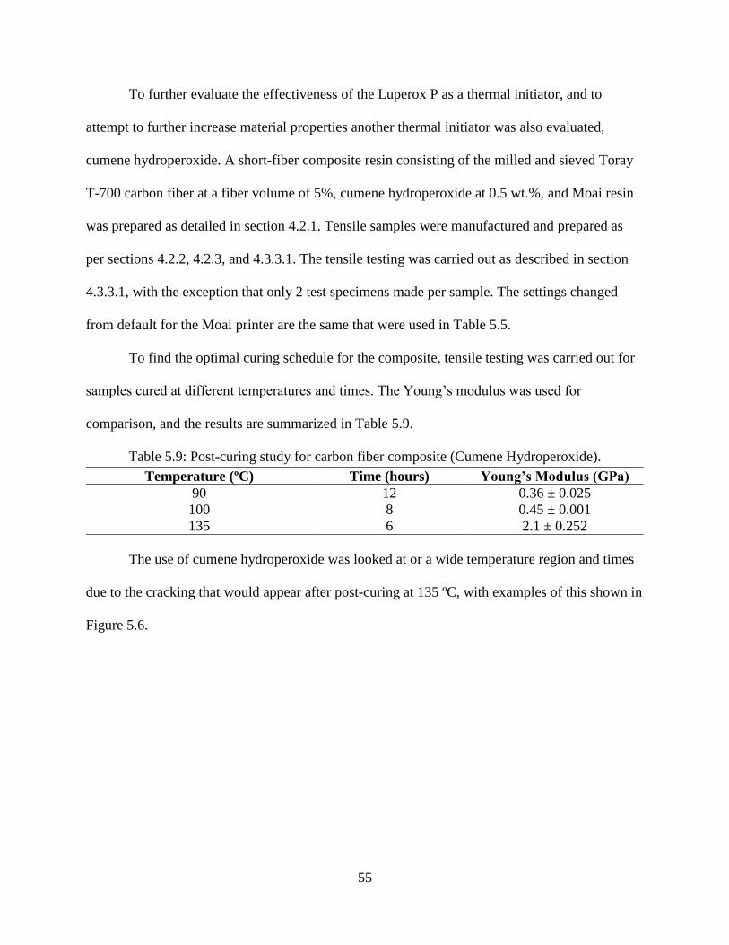
55

To further evaluate the effectiveness of the Luperox P as a thermal initiator, and to

attempt to further increase material properties another thermal initiator was also evaluated,

cumene hydroperoxide. A short-fiber composite resin consisting of the milled and sieved Toray

T-700 carbon fiber at a fiber volume of 5%, cumene hydroperoxide at 0.5 wt.%, and Moai resin

was prepared as detailed in section 4.2.1. Tensile samples were manufactured and prepared as

per sections 4.2.2, 4.2.3, and 4.3.3.1. The tensile testing was carried out as described in section

4.3.3.1, with the exception that only 2 test specimens made per sample. The settings changed

from default for the Moai printer are the same that were used in Table 5.5.

To find the optimal curing schedule for the composite, tensile testing was carried out for

samples cured at different temperatures and times. The Young’s modulus was used for

comparison, and the results are summarized in Table 5.9.

Table 5.9: Post-curing study for carbon fiber composite (Cumene Hydroperoxide).

Temperature (ºC) Time (hours) Young’s Modulus (GPa)

90 12 0.36 ± 0.025

100 8 0.45 ± 0.001

135 6 2.1 ± 0.252

The use of cumene hydroperoxide was looked at or a wide temperature region and times

due to the cracking that would appear after post-curing at 135 ºC, with examples of this shown in

Figure 5.6.

56

Figure 5.6: Cracks in cumene hydroperoxide post-cured specimens.

The cracks would run both parallel (front of specimen) and perpendicular (side of

specimen) to the loading direction of the tensile testing. This resulted in the low modulus seen

due to system compliance [44]. At lower temperatures the thermal initiator would not activate

and fully cure the sample. This can be seen in Table 5.9 from the low results of the Young’s

modulus.

5.2.3. Fiber Volume Consistency and Porosity

5.2.3.1. Fiber Volume Consistency

The fiber volume consistency was evaluated as outlined in section 4.3.6. The results

summarized in Table 5.10, with the full results in APPENDIX A, Table A.1 and Table A.2.

Table 5.10: Summarized fiber volume consistency results for flexural samples.

Layer Height (μm) Print Time (hours) Top (% Vf) Middle (% Vf) Bottom (% Vf)

100 3.0 5.23 ± 0.02 4.84 ± 0.10 3.57 ± 0.27

50 5.25 5.45 ± 0.15 4.50 ± 0.13 3.88 ± 0.01

From Table 5.10 it can be seen that a fiber volume gradient is present with in the

samples. The top section of the samples have a higher fiber volume then what the resin mixture

was designed to have (5% Vf). This is due to the lowering of the bed plate into the vat trapping

57

more fibers in-between the sample and bottom of the vat then desired. The reason believed for

the samples to have lower and similar fiber volume gradients despite the different print times, is

that the area around the sample being printed becomes depleted of fibers as the sample is printed.

This slowly lowers the fiber volume of the sample as it is going through the printing process. The

possible effects of this fiber volume gradients effect on the material properties will be discussed

in the following Material Characterization section 5.2.4.

Because the flexural specimens have a larger cross-section area throughout the entire

specimen the fiber gradient appears more pronounced. Similar burn off testing was carried out

with the tensile specimens (geometry shown in Figure 4.10) with the exception that only the two

ends were tested. This was done early on in the manufacturing process to evaluate the

consistence of the print process. The average difference in the fiber volume of the top and

bottom portions of the tensile specimens change by on average of 0.8% for the specimens printed

in the 90º orientation. This lower difference could be to the varying specimen geometry, or that

due to their large size a less number of specimens were printed at the same time to keep the print

time short. This allowed for more spacing between the specimens, and could have prevented the

fiber from becoming depleted from around the specimens being printed.

The Moai printer has no built in mixing method such as a pump or wiper arm that can be

found in some other manufactures printers. To facilitate mix of the resin the setting for the

distance the vat tilts (PM Reset Position) when the peel step occurs was increased from the

default setting of 40 to 50. While this did aid in recoating the vat surface, the gradient in the fiber

volume was still present in the samples. Increasing this value can also had the negative effect of

increasing the peel force on the parts therefore limiting the amount it can be increased. During

the course of this research attempts were made to incorporate a pump into the resin vat were

58

made, but the effort was unsuccessful. This was mainly due to the limited amount of space to

incorporate the necessary equipment. Recommendations for a solution to the problem of fiber

volume consistency are presented in the Future Recommendations section 6.2.

5.2.3.2. Composite Porosity

The results of the void content testing along with the densities, outlined in section 4.3.7,

are summarized in Table 5.11, with the full results for the testing in APPENDIX A, Table A.4.

Table 5.11: Density and void content of composite samples.

Layer Height Sample Density

(g/cm3)

Void Content

(%)

100 μm 5% Vf Carbon Fiber + 0.5 wt.% Luperox P 1.25 1.32

50 μm 5%Vf Carbon Fiber + 0.5 wt.% Luperox P 1.25 0.70

100 μm 0.5 wt.% Luperox P 1.24 -

The voids present in the composite samples can originate both during the manufacturing

of the fiber reinforced resin used for printing and during the printing of the samples. Although

the resin was degassed in a vacuum chamber before using there could still be air trapped in the

resin and to the fibers themselves. Voids can be introduced during the peel step between every

layer when the sample is raised up from the vat. During the photo polymerization process the

volume of the liquid resin is reduced when going to a solid. This leaves behind a negative space

that can then form bubbles that are trapped in the liquid resin, and then be incorporated into the

sample. This was observed in some of the Moai resin samples before parameters were adjusted

by allowing the vat and bed to separate more in-between layers. The Moai resin parts are

transparent so any samples with visible voids could be removed from testing and reprinted. For

the samples made with carbon fiber, they are not transparent and therefore it could be possible

for samples with voids formed due to this manufacturing defect to still be used as testing

specimens.

59

The voids could also be due to the thermal initiator producing gas byproducts during the

post-curing process [61]. With the 100 μm layer height having more unreacted resin from the

photo polymerization process then the 50 μm layer height, with this being elaborated on more in

the following section 5.2.4.1. This could be why the 100 μm layer height was seen to have a

higher void content than that of the 50 μm layer height samples. The presence of voids within the

composite will act as stress concentrators, but a 1% void content is considered good whereas

around 5% would be considered poor for traditional laminate composites [13].

5.2.4. Material Characterization

5.2.4.1. Tensile Testing

A short-fiber composite resin consisting of the milled and sieved Toray T-700 carbon

fiber at a fiber volume of 5%, Luperox P at 0.5 wt.%, and Moai resin was prepared as detailed in

section 4.2.1. Tensile samples were manufactured and prepared as per sections 4.2.2, 4.2.3, and

4.3.3.1. The tensile testing was carried out as described in section 4.3.3.1, with the exception the

test numbers 4,8,12, and 16 from Table 4.7 were left out. The test omitted represent the samples

made with carbon fiber and no thermal initiator, which was shown as ineffective in section 5.1.1.

The settings changed from default for the Moai printer are the same that were used in Table 5.5,

unless otherwise stated.

It was found the by applying a thin layer of neat Moai resin to the print bed before

starting the print aided in keeping the part fixed to the bed during the printing process. The thin

layer of neat resin was able to cure more during the over exposer processes during the first few

layers. When no neat resin was applied to the bed before printing some specimens would become

unattached from the bed during the peel step, resulting in print failure. The success rate of prints

60

with the thin layer of neat resin applied to the bed was greatly increased, and would be

recommend for any future research with this style of SLA printer to aid in part success.

To aid in sample identification the follow naming scheme will be implemented for the

remainder of this paper. It will consist of the main material parameter being looked at along with

the layer height and print orientation, shown in Table 5.12.

Table 5.12: Sample identification guide.

Abbreviation Sample Components Layer Height Print Orientation

M100-0 Moai Resin 100 0º




LP100-0 Moai Resin + 0.5 wt.% Luperox P 100 0º




CF100-0 Moai Resin + 0.5 wt.% Luperox P +

5% Vf Carbon Fiber

100 0º


5% Vf Carbon Fiber

100 90º


5% Vf Carbon Fiber

50 0º


5% Vf Carbon Fiber

50 90º

The maximum tensile strength and Young’s modulus was found as specified in ASTM

D638 section 11.2 and 11.4 respectively, and the results are shown in Figure 5.7, Figure 5.8,

Figure 5.9, Figure 5.10, and summarized in Table 5.13 [48]. The results for the samples printed

in the 0º orientation are shown in Figure 5.7 and Figure 5.8., and the samples printed in the 90º

orientation are shown in Figure 5.9 and Figure 5.10.

61

Figure 5.7: Tensile strength results for 0º print orientation.

Figure 5.8: Young's modulus results for 0º print orientation.

62

Figure 5.9: Tensile stregnth results for 90º print orientation.

Figure 5.10: Young's modulus results for 90º print orientation.

63

Table 5.13: Summarized tensile testing results.

Sample Layer Height

(µm)

Print

Orientation

Fiber

Volume

(%)

Tensile

Strength

(MPa)

Young’s

Modulus

(GPa)

M100-0 100 0° 0 58.9 ± 5.0 2.72 ± 0.06

M100-90 100 90º 0 66.1 ± 0.4 2.87 ± 0.05

M50-0 50 0° 0 43.4 ± 7.7 2.81 ± 0.15

M50-90 50 90º 0 64.6 ± 1.6 2.89 ± 0.12

LP100-0 100 0° 0 36.9 ± 7.9 3.17 ± 0.15

LP100-90 100 90º 0 22.5 ± 22.5 3.17 ± 0.26

LP50-0 50 0° 0 50.3 ± 7.7 3.04 ± 0.11

LP50-90 50 90º 0 68.8 ± 5.9 2.83 ± 0.01

CF100-0 100 0° 5 52.4 ± 3.7 3.29 ± 0.29

CF100-90 100 90º 5 41.4 ± 2.6 3.39 ± 0.52

CF50-0 50 0° 5 50.6 ± 6.6 3.46 ± 0.17

CF50-90 50 90º 5 11.69 ± 2.28 2.92 ± 0.01

When comparing the Young’s modulus of the samples there was an increase of 21%

between the M100-0 and CF100-0 samples, and an increase of 27% for the M50-0 and the CF50-

0. With an increase in Young’s modulus for the CF50-0 samples when compared to the CF100-0

of 5%. While showing only 4% increase between the LP100-0 and CF100-0 samples, and 13%

increase for the LP50-0 and CF50-0. These increase in the Young’s modulus are not as high as

what would be predicted theoretically using Equations 2.2 thru 2.6 for a randomly distributed

short-fiber composite (CF100 samples). Using the average fiber length, found in section 5.2.2.1,

of 76 μm the theoretical modulus for a randomly distributed composite would be 4.05 GPa, and

for a unidirectional composite it would be 5.42 GPa.

The theoretical modulus for the randomly distributed composite is 23% higher than that

of the CF100-0 sample. This is in part due to the distribution of the shorter fiber lengths within

the sample, but also that the theoretical model also assumes perfect bonding between the fiber

and matrix along with an absents of voids [13]. Evidence of the weak interfacial properties of the

short-fiber composite samples can be seen in Figure 5.11.

64

Figure 5.11: Fracture surface of CF50-0 (A) X200 and (B) X250 magnification.

In Figure 5.11, the smooth channels left behind from the carbon fiber in A, the clean

(lack of bonded matrix material) fibers present in B, and the smooth holes in B are all signs of

weak interfacial properties due to poor bonding between the matrix and fiber [13, 60]. This limits

the ability for the matrix to transfer stress to the fibers and therefore reducing its overall

properties [13]. If the composite had better interfacial properties there would have been evidence

of fiber breakage, which was not present in any of the SEM Images taken [13, 60]. The results of

the fiber volume consistence (section 5.2.3.1) showed that a fiber volume gradient existed in the

samples produced, but the gage section of the tensile sample is in the middle of the print were the

fiber volume should be more uniform, due to the lower difference found between the top and

bottom of the tensile specimen fiber volume content (0.8%).

When comparing the modulus of the carbon fiber samples printed at different layer

heights (100 μm and 50 μm) the increase in modulus of 5% can be attributed to the partial

alignment of the fibers in the loading direction. While the CF100-90 has a higher modulus than

the CF50-90 samples. While this would be expected if the material was going from isotropic

material to a special orthotropic material due to fiber alignment, it is not the case for these

65

samples due to cracks being present in the CF50-90 samples [13]. The cracks presence and their

effect in the CF50-90 samples will be discussed in greater detail later in this section. The

alignment of the fibers via layer height is demonstrated in Figure 5.12 with the yellow arrows

highlighting the various fiber orientations.

Figure 5.12: Fracture surface of (A) CF100-90 and (B) CF50-90 specimens.

When comparing the strength of the Moai resin samples, the samples printed in the 90º

print orientation for the Moai resin have a higher strength when compared to the same samples

printed in the 0º print orientation. This is due to the effects of the support material being removed

and leaving behind notches in the specimen, examples of this can be seen in Figure 4.7 in section

4.2.3. These notches then act as small stress concentrators resulting in lower strength of the

sample [44]. Due to these effects the Moai resin samples tested at a print orientation of 90º are a

better representation of the actual ultimate tensile strength of the neat resin material.

The samples tested with just the thermal initiator (Luperox P) added also showed flaws

the contributed to a lower tensile strength result. These are from cracks there were present on the

66

surface of the samples that originated during the curing process, with an example of these defects

shown in Figure 5.13.

Figure 5.13: Surface cracking from thermal curing.

The cracks originate from the volumetric shrinkage that occurs during the post-curing

process as the degree of conversation within the system increases [62]. A slower curing schedule

might be able to produce samples without cracks, but it was keep the same as the carbon fiber

samples for comparison purposes. The volumetric shrinkage due to post-curing was found for the

different samples as outlined in section 4.3.8. The results for the volumetric change in the

samples from post-curing are summarized in Table 5.14, with the full results in APPENDIX A,

Table A.5 thru Table A.10.

Table 5.14: Volumetric shrinkage (%) of post-cured samples.

Sample Volume Shrinkage (%)

M100 1.4 ± 0.6

LP100 3.5 ± 0.6

CF100 1.1 ± 0.8

M50 0.8 ± 0.5

LP50 1.0 ± 0.7

CF50 0.4 ± 0.3

67

The largest change in volume can be seen in the LP-100 sample, and the largest decrease

in strength can be seen in the LP100-0 and LP100-90 samples. The LP-100 tension samples also

showed the largest number of cracks when compared to the LP50-0 and LP50-90 samples. This

is due to the dual-cure system working against itself. When the samples are first cured rapidly

using the photo initiator the polymer quickly becomes fixed in place at a low degree of

conversation [62]. During the post-curing process the thermal initiator then reacts with remaining

function groups increasing the shrinkage and therefore stress within the sample causing cracks to

develop [62]. This is more pronounced in the samples at a 100 μm layer height due to there being

more unreacted material for the thermal initiator to react with, due to the lower degree of

conversion from less energy being delivered to the photo initiator [32, 62]. This can also be seen

in SEM images taken from the fracture surfaces of the tensile specimens. Figure 5.14 is of the

fracture surface of a M100-90 specimen.

Figure 5.14: M100-90 fracture surface at (A) X500 and (B) X1000 magnification.

From Figure 5.14 the fracture appears as brittle until increasing the magnification and

then areas of plastic deformation can be seen, and indicating more of a ductile failure on a

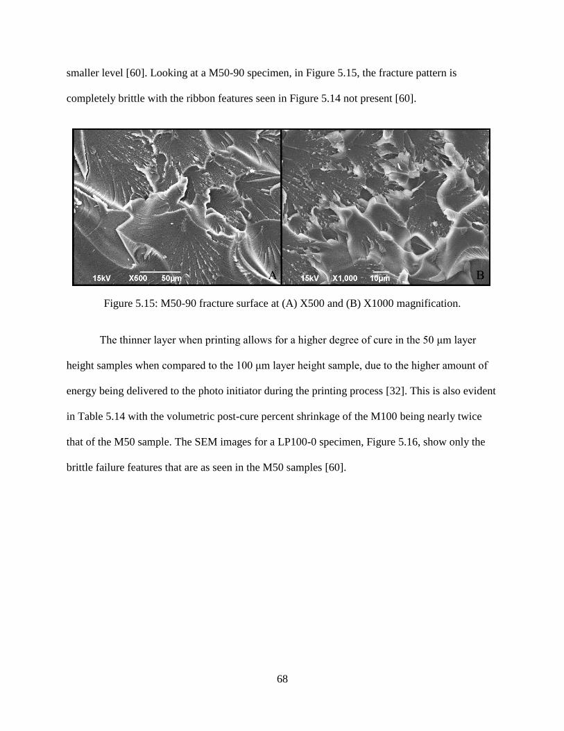
68

smaller level [60]. Looking at a M50-90 specimen, in Figure 5.15, the fracture pattern is

completely brittle with the ribbon features seen in Figure 5.14 not present [60].

Figure 5.15: M50-90 fracture surface at (A) X500 and (B) X1000 magnification.

The thinner layer when printing allows for a higher degree of cure in the 50 μm layer

height samples when compared to the 100 μm layer height sample, due to the higher amount of

energy being delivered to the photo initiator during the printing process [32]. This is also evident

in Table 5.14 with the volumetric post-cure percent shrinkage of the M100 being nearly twice

that of the M50 sample. The SEM images for a LP100-0 specimen, Figure 5.16, show only the

brittle failure features that are as seen in the M50 samples [60].

69

Figure 5.16: LP100-0 fracture surface at (A) X500 and (B) X1000 magnification.

The samples with carbon fiber on the other hand, show similar shrinkage as the Moai

resin samples even though there would be unreacted resin due to the shadowing of the carbon

fiber from the UV light source. The lower shrinkage of the carbon fiber samples is due to the

carbon fiber providing dimensional stability to the samples during the curing process by limiting

their thermal expansion, and the volume of the carbon fiber displacing some of the volume of the

resin when compare to the original volume of resin in neat Moai samples [13, 32].

The lower strength of the carbon fiber samples is due in part by the end effects of the

fiber reinforcement acting as stress concentrators within the composite [13]. This is caused by

the large number of very short fibers (much less than the critical length) in the distribution of the

lengths, seen in Figure 5.4, being present in the sample [13]. The presence of voids with in the

carbon fiber samples can also act as stress concentrators and farther weaken the samples, but the

low void content found (section 5.2.3.2) for the samples should help minimize the effect [63].

The cracks seen on the surface of the LP100 and LP50 samples were not seen in the

carbon fiber samples, but the CF50-90 sample did have cracks present before post-curing from

the printing processes itself, examples of these cracks are shown in Figure 5.17.

70

Figure 5.17: Cracks in CF50-90 sample from printing.

This was caused due to the smaller layer height not having as much matrix material

available for holding one layer to the next. During the peel step of the printing process, when the

part would be separated from the silicon layer on the bottom of the vat, it would generate enough

stress to separate previous layers. Multiple attempts to print the CF50-90 specimens resulted in

failures due to the layers sticking to the bottom of the vat instead of the printed part itself.

Examples of these failures shown in Figure 5.18.

Figure 5.18: Examples of CF50-90 print failures.

71

From Figure 5.18, the cone shaped failures in the print are from a small piece of a layer

separating from the part and sticking to the vat, as the subsequent layers are printed this small

piece sticking to the vat slowly increase in size until causing printing failure. To overcome this

and manufacture specimens that could be tested the PM motor speed was lowered until part

failure no longer occurred, this was found to be a value of 6 for the Moai printer settings. By

lowering the speed of the PM motor it deceased the force generated of the part during the peel

step, but could not completely remove it resulting in the cracks seen in the specimens. The cracks

being present in the specimens caused a large decrease in the strength of the CF50-90 samples

due to the cracks decreasing in the actual cross-sectional area and acting as stress concentrators

[44]. While also decreasing the Young’s modulus by increasing the compliance of the specimens

[44].

The strength of the short-fiber composites were also affected by the length of the carbon

fiber being used. To get the maximum amount of reinforcement from the carbon fiber the fiber

needs to be over a critical length, lc, to maximize the load transfer between the fiber and matrix

[13]. This can be found for the current composite system by solving Equation 2.1, with the fiber

properties given in Table 4.3, and assuming a shear yield stress of the matrix to be half of the

tensile strength of the matrix with the critical fiber length for this system being 434 μm [13]. The

shorter length of the fibers (76 μm) being used means that the load is not being fully transferred

to the fiber, and limiting the composites performance [13].

The statistical analysis for the tensile testing results for the Young’s modulus and

ultimate tensile strength of the evaluated materials is examined in the following two sections, as

outlined in section 4.3.3.2

72

5.2.4.1.1. Young’s Modulus

The results for the Young’s modulus for the samples tested were evaluated using

ANOVA and if needed a post-hoc Tukey HSD test, as outlined in section 4.3.3.2. The samples

were compared across 4 different groups these were, 0º and 90º print orientation and 100 μm and

50 μm layer heights. The groups analyzed are shown in Table 5.15.

Table 5.15: Statistical analysis groups.

Group

Parameter Groups

0º Print

Orientation M100-0 LP100-0 CF100-0 M50-0 LP50-0 CF50-0

90º Print

Orientation M100-90 LP100-90 CF100-90 M50-90 LP50-90 CF50-90

100 μm Layer

Height M100-0 LP100-0 CF100-0 M100-90 LP100-90 CF100-90

50 μm Layer

Height M50-0 LP50-0 CF50-0 M50-90 LP50-90 CF50-90

The results for the ANOVA analysis when comparing samples in the 0º print orientation

are summarized in Table 5.16, with the full ANOVA results in Table B.1 in APPENDIX B.

Table 5.16: ANOVA summary for Young's modulus in 0º print orientation.

Source of

Variation

Sum of

Squares

Degrees

of

Freedom

Mean

Square F-Statistic P-value F-Critical

Between

Groups 1.99 5 0.398 13.84 2.05*10-6 2.62

Within

Groups 0.691 24 0.0288 - - -

The ANOVA result were also plotted in MatLab as notched box plots for visual

examination of the data, and is shown in Figure 5.19.

73

Figure 5.19: Box plot of ANOVA results for Young's modulus in 0º print orientation.

From the results of the ANOVA testing the p-value of 2.05*10-6 is less than that of 0.05

for the 95% confidence level chosen. This indicates that there is significant differences between

at least two of the means in the sample groups tested [50]. From Figure 5.19 a visual

determination can be made to determine which groups differ, and it can be seen that there is

some separation between the notches in the box plots of the samples. The summarized results of

the Tukey test for the 0º sample groups that showed significant differences are shown in Table

5.17, with the full Tukey results in APPENDIX B, Table B.2.

2.6

2.8

3

3.2

3.4

3.6

M100-0 LP100-0 CF100-0 M50-0 LP50-0 CF50-0Sample

Mo

du

lus

(GP

a)

74

Table 5.17: Tukey HSD results for Young's modulus in 0º print orientation.

Compared Pairs Tukey HSD Q

statistic Tukey HSD p-value

Tukey HSD

inference

M100-0 vs LP100-0 5.9817 0.0035542 p<0.01

M100-0 vs CF100-0 7.4633 0.0010053 p<0.01

M100-0 vs CF50-0 9.7304 0.0010053 p<0.01

LP100-0 vs M50-0 4.7848 0.0262724 p<0.05

CF100-0 vs M50-0 6.2664 0.0021738 p<0.01

M50-0 vs CF50-0 8.5336 0.0010053 p<0.01

LP50-0 vs CF50-0 5.5414 0.0075388 p<0.01

From Table 5.17, both CF100-0 and CF50-0 differ statistically and have higher moduli

then the M100-0 and M50-0 moduli, respectively. The results also show that the LP100-0 does

not differ from the CF100-0 or the CF50-0. This is in part due to the large deviation with in the

CF100-0 sample. This indicates that somewhere within the processing parameters something is

causing a deviation with in the manufacturing of the samples [50]. This could be due to things

such as fiber distribution, voids, or other unseen imperfections in the sample, with solutions for

these issues proposed in later sections. This can be seen with the CF50-0 being statistical

different than the LP50-0, due to the smaller deviation within the confidence interval of the

CF50-0 samples when compared to the CF100-0 samples.



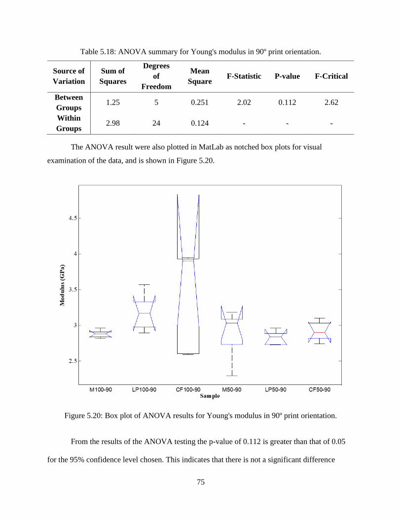
75

Table 5.18: ANOVA summary for Young's modulus in 90º print orientation.

Source of

Variation

Sum of

Squares

Degrees

of

Freedom

Mean


Between

Groups 1.25 5 0.251 2.02 0.112 2.62

Within

Groups 2.98 24 0.124 - - -



Figure 5.20: Box plot of ANOVA results for Young's modulus in 90º print orientation.

From the results of the ANOVA testing the p-value of 0.112 is greater than that of 0.05

for the 95% confidence level chosen. This indicates that there is not a significant difference

76

between the sample groups tested [50]. From Figure 5.20, a visual determination can be made to

confirm that the groups do not differ, and it can be seen that there is overlap between all of the

samples within the 95% confidence level, represented by the ends of the notches. This is in part

due to the large deviation with in the CF100-90 sample. As was mentioned before with the

CF100-0, this is due to inconsistences within the printing process. If this deviation could be

corrected for more consistent samples then the CF100-90 would be statistical different than the

other samples tested. This is seen in the box plots median value (3.90 GPa) for the CF100-90

being higher than its mean value (3.39 GPa), and highlights the potential for improvement in the

material properties. For completeness, the Tukey HSD test was still carried out with none of the

results indicating any significant differences. The results of the Tukey test for the 90º sample

groups can be found in APPENDIX B, Table B.4.

The results for the ANOVA analysis when comparing samples printed at a 100 μm layer

height are summarized in Table 5.19, with the full ANOVA results in Table B.5 in APPENDIX

B.

Table 5.19: ANOVA summary for Young's modulus printed at 100 μm layer height.

Source of

Variation

Sum of

Squares

Degrees

of

Freedom

Mean


Between

Groups 1.63 5 0.326 2.78 0.0404 2.62

Within

Groups 2.81 24 0.117 - - -



77

Figure 5.21: Box plot of ANOVA results for Young's modulus printed at 100 μm layer height.

From the results of the ANOVA testing the p-value of 0.0404 is less than that of 0.05 for

the 95% confidence level chosen. This indicates that there is significant differences between at

least two the sample groups tested [50]. From Figure 5.21, a visual determination can be made to

determine which groups differ, and that there is some separation between the means of the

samples, but with most of the notches overlapping. This is again due to the large standard of

deviation, and therefore large spread in data of the CF100-90 samples. The summarized results

of the Tukey test for the 100 μm layer height sample groups that showed significant differences

are shown in Table 5.20, with the full Tukey results in APPENDIX B, Table B.6.

78

Table 5.20: Tukey HSD results for Young's modulus printed at 100 μm layer height.



Tukey HSD

inference

M100-0 vs CF100-90 4.3934 0.0484687 p<0.05

While the Tukey results only should a difference between the M100-0 and CF 100-90, if

the deviation of the CF 100-90 sample could be reduced it might have showed a difference

between all of the other groups. The higher median of the CF100-90 than that of the CF 100-0

also shows that at layer heights larger than the average fiber length isotropic parts possibly could

be produced. If fiber was being aligned more in plane with the printing surface it would be

expected that the properties would have been lower than the CF 100-0 results [13].



B.

Table 5.21: ANOVA summary for Young's modulus printed at 50 μm layer height.

Source of

Variation

Sum of

Squares

Degrees

of

Freedom

Mean


Between

Groups 1.49 5 0.298 8.31 1.13*10-4 2.62

Within

Groups 0.86 24 0.0358 - - -



79

Figure 5.22: Box plot of ANOVA results for Young's modulus printed at 50 μm layer height.



at least two of the sample groups tested [50]. From Figure 5.22, there is some separation between

the means of the samples, but most of the notches overlap with CF50-0 showing the greatest

difference. The summarized results of the Tukey test for the 50 μm layer height sample groups

that showed significant differences are shown in Table 5.22, with the full Tukey results in

APPENDIX B, Table B.8.

80

Table 5.22: Tukey HSD results for Young's modulus printed at 50 μm layer height.

Treatments Pair Tukey HSD Q

Statistic

Tukey HSD p-

value

Tukey HSD

Inference

M50-0 vs CF50-0 7.6447 0.0010053 p<0.01

LP50-0 vs CF50-0 4.9642 0.0196729 p<0.05

CF50-0 vs M50-90 6.752 0.0010053 p<0.01

CF50-0 vs LP50-90 7.5148 0.0010053 p<0.01

CF50-0 vs CF50-90 6.3954 0.001736 p<0.01

M50-0 vs CF50-0 7.6447 0.0010053 p<0.01

The CF50-0 shows the greatest difference between the different samples, which is a good

indicator that the carbon fiber is working as a reinforcement for the resin. The CF50-90 would be

predicted to be lower than the CF50-0 if fiber alignment was as such that the load was being

applied out of plane of a special orthotropic composite, it is more likely due to the cracks that

were present in the sample as discussed in the previous section [13].

5.2.4.1.2. Tensile Strength

The results for the ultimate tensile strength for the samples were evaluated using

ANOVA and if needed a post-hoc Tukey HSD test, as outlined in section 4.3.3.2. The samples

were compared across 4 different groups, 0º and 90º print orientation and 100 μm and 50 μm

layer heights. The groups analyzed are the same that were used in the statistical analysis for the

Young’s modulus, and are shown in Table 5.15.



81

Table 5.23: ANOVA summary for tensile strength in 0º print orientation.

Source of

Variation

Sum of

Squares

Degrees

of

Freedom

Mean


Between

Groups 1465.0 5 293.0 6.58 5.515*10-4 2.62

Within

Groups 1069.4 24 44.6 - - -



Figure 5.23: Box plot of ANOVA results for tensile strength in 0º print orientation.



82

the sample groups tested [50]. From Figure 5.23, a visual determination can be made to

determine which groups differ, and from these box plots it can be seen that there is some

separation between the means of the samples. The summarized results of the Tukey test for the 0º

sample groups that showed significant differences are shown in Table 5.24, with the full Tukey

results in APPENDIX B, Table B.10.

Table 5.24: Tukey HSD results for tensile strength in 0º print orientation.



Tukey HSD

inference

M100-0 vs LP100-0 7.4069 0.0010053 p<0.01

M100-0 vs M50-0 5.1935 0.0135044 p<0.05

LP100-0 vs CF100-0 5.2144 0.0130433 p<0.05

LP100-0 vs LP50-0 4.5001 0.0411466 p<0.05

LP100-0 vs CF50-0 4.5967 0.0353984 p<0.05

As discussed in section 5.2.4.1, the samples printed in the 0º orientation strengths are

lowered by the defects left from removal of the support material, and the cracks present in the

LP100 and LP50 samples. The samples printed in the 90º print orientation are better

representations of the neat Moai resin strength.



Table 5.25: ANOVA summary for tensile strength in 90º print orientation.

Source of

Variation

Sum of

Squares

Degrees

of

Freedom

Mean


Between

Groups 14521.5 5 2904.3 31.17 9.49*10-10 2.62

Within

Groups 2236.1 24 93.2 - - -

The ANOVA result were also plotted in MatLab as box plots for visual examination of

the data, and is shown in Figure 5.24.

83

Figure 5.24: Box plot of ANOVA results for tensile strength in 90º print orientation.


for the 95% confidence level chosen. This indicates that there is significant difference between

the sample groups tested [50]. From Figure 5.24, many of the sample means do not overlap, but

the red cross present above LP100-90 is an indication of an outlier. Although it is an outlier it is

most likely a better reflation of the strength of the LP-100 sample. This is due to all the cracks

that were present in the samples with just Luperox P added, but was not as prevalent in the

specimen that produced that data point. In Figure 5.24, the size of the confidence interval

(notches) are smaller than what is seen in Figure 5.23 due to the defects of the supports not being

present on the specimens. The summarized results of the Tukey test for the 90º sample groups

84

that showed significant differences are shown in Table 5.26, with the full Tukey results in


Table 5.26: Tukey HSD results for tensile strength in 90º print orientation.


Statistic

Tukey HSD p-

value

Tukey HSD

Inference

M100-90 vs LP100-90 9.473 0.0010053 p<0.01

M100-90 vs CF100-90 6.2817 0.0021166 p<0.01

M100-90 vs CF50-90 13.1663 0.0010053 p<0.01

LP100-90 vs M50-90 8.5619 0.0010053 p<0.01

LP100-90 vs LP50-90 9.5533 0.0010053 p<0.01

CF100-90 vs M50-90 5.3706 0.0100509 p<0.05

CF100-90 vs LP50-90 6.362 0.0018398 p<0.01

CF100-90 vs CF50-90 6.8846 0.0010053 p<0.01

M50-90 vs CF50-90 12.2552 0.0010053 p<0.01

LP50-90 vs CF50-90 13.2466 0.0010053 p<0.01

The lower strength of the carbon fiber and Luperox samples when compared to the Moai

resin have been discussed in the previous section 5.2.4.1, and are a result of poor interface

strength and stress concentration effects.


height are summarized in Table 5.27, with the full ANOVA results in Table B.13, in APPENDIX

B.

Table 5.27: ANOVA summary for tensile strength printed at 100 μm layer height.

Source of

Variation

Sum of

Squares

Degrees

of

Freedom

Mean


Between

Groups 5714.6 5 1142.9 11.08 1.29*10-5 2.62

Within

Groups 2474.7 24 103.1 - - -



85

Figure 5.25: Box plot of ANOVA results for tensile strength printed at 100 μm layer height.



at least two of the sample groups tested [50]. From Figure 5.25, there is separation between the

many of the means of the samples, with the outlier from LP50-90 present again. The summarized

results of the Tukey test for the 100 μm layer height sample groups that showed significant

differences are shown in Table 5.28, with the full Tukey results in APPENDIX B, Table B.14.

86

Table 5.28: Tukey HSD results for tensile strength printed at 100 μm layer height.



Tukey HSD

inference

M100-0 vs LP100-0 4.8691 0.0229462 p<0.05

M100-0 vs LP100-90 6.9028 0.0010053 p<0.01

LP100-0 vs M100-90 6.9711 0.0010053 p<0.01

CF100-0 vs LP100-90 5.4615 0.0086307 p<0.01

M100-90 vs LP100-90 9.0048 0.0010053 p<0.01

M100-90 vs CF100-90 5.9712 0.0036196 p<0.01

Again the Moai resin samples have a higher strength, but the carbon fiber reinforced

samples for both the 0º and 90º print orientation are not statistically different. This helps

demonstrates that for a layer height larger than the length of the fiber an isotropic part could be

manufactured.



B.

Table 5.29: ANOVA summary for tensile strength at 50 μm layer height.

Source of

Variation

Sum of

Squares

Degrees

of

Freedom

Mean


Between

Groups 10307.4 5 2061.5 59.55 9.67*10-13 2.62

Within

Groups 830.8 24 34.6 - - -



87

Figure 5.26: Box plot of ANOVA results for tensile strength printed at 50 μm layer height.



the sample groups compared [50]. From Figure 5.26, while the CF50-0 looks to be of the same

strength as the M50-0, but the values could be affected due to the support material defects being

present in the specimens. The summarized results of the Tukey test for the 50 μm layer height



88

Table 5.30: Tukey HSD results for tensile strength printed at 50 μm layer height.


Statistic

Tukey HSD p-

value

Tukey HSD

Inference

M50-0 vs M50-90 8.0251 0.0010053 p<0.01

M50-0 vs LP50-90 9.6515 0.0010053 p<0.01

M50-0 vs CF50-90 12.0803 0.0010053 p<0.01

LP50-0 vs M50-90 5.4311 0.0090823 p<0.01

LP50-0 vs LP50-90 7.0574 0.0010053 p<0.01

LP50-0 vs CF50-90 14.6744 0.0010053 p<0.01

CF50-0 vs M50-90 5.3215 0.0109131 p<0.05

CF50-0 vs LP50-90 6.9478 0.0010053 p<0.01

CF50-0 vs CF50-90 14.784 0.0010053 p<0.01

M50-0 vs LP50-0 20.1054 0.0010053 p<0.01

M50-0 vs CF50-0 21.7318 0.0010053 p<0.01

The poor results from the CF50-90 causes a larger difference between the groups then

would otherwise be present, but the trend of the 90º oriented parts having higher strengths is still

present for the other samples, from the support material not being present in the gage section.

5.2.4.2. Flexural Testing



section 4.2.1. Flexural samples were manufactured and prepared as per sections 4.2.2, 4.2.3, and

4.3.4.1. The flexural testing was carried out as described in section 4.3.4.1, with the exception

the test numbers 4,8,12, and 16 from Table 4.10 were left out. The test numbers omitted

represent the samples made with carbon fiber and no thermal initiator which was shown as

ineffective in section 5.1.1. The settings changed from default for the Moai printer are the same

that were used in Table 5.5 unless otherwise stated. As in section 5.2.4.1, a thin layer of neat

Moai resin to the print bed before starting the print aided in keeping the part fixed to the bed

during the printing process. With the same naming convention used for the samples as shown in

Table 5.12.

89

The maximum flexural strength and flexural modulus was found as specified in ASTM

D790 section 12.2 and 12.5 respectively, and the results are shown in Figure 5.27, Figure 5.28,

Figure 5.29, and Figure 5.30, and summarized in Table 5.31 [53]. The results for the samples

printed in the 0º orientation are shown in Figure 5.27 and Figure 5.28, for the flexural strength

and flexural modulus respectively, and for the samples printed in the 90º shown in Figure 5.29

and Figure 5.30, for the flexural strength and flexural modulus respectively.

Figure 5.27: Flexural strength results for 0º print orientation.

90

Figure 5.28: Flexural modulus results for 0º print orientation.

Figure 5.29: Flexural stregnth results for 90º print orientation.

91

Figure 5.30: Flexural modulus results for 90º print orientation.

Table 5.31: Summarized flexural testing results.

Sample Layer Height

(µm)

Print

Orientation

Fiber

Volume

(%)

Flexural

Strength

(MPa)

Flexural

Modulus

(GPa)

M100-0 100 0° 0 86.0 ± 9.5 2.52 ± 0.07

M100-90 100 90º 0 96.2 ± 1.7 2.42 ± 0.01

M50-0 50 0° 0 82.2 ± 11.2 2.42 ± 0.05

M50-90 50 90º 0 100.8 ± 3.4 2.62 ± 0.06

LP100-0 100 0° 0 27.9 ± 5.4 2.34 ± 0.15

LP100-90 100 90º 0 14.6 ± 3.0 2.47 ± 0.21

LP50-0 50 0° 0 23.9 ± 3.7 2.55 ± 0.23

LP50-90 50 90º 0 13.2 ± 0.6 2.50 ± 0.20

CF100-0 100 0° 5 84.9 ± 4.3 2.59 ± 0.06

CF100-90 100 90º 5 66.1 ± 10.5 2.31 ± 0.11

CF50-0 50 0° 5 43.4 ± 5.5 2.64 ± 0.12

CF50-90 50 90º 5 19.4 ± 2.5 2.58 ± 0.16

Overall the flexural modulus of the samples were not improved by the addition of the

carbon fiber. This could be primarily due to the lower fiber volume (5%) of the samples, causing

them to have results similar to that of the neat resin samples. During the flexural testing the

specimens are subjected to the more complex stress state (compressive, tensile, and shear) when

92

compared to the previous tensile stress state from the axial testing in section 5.2.4.1 [63, 64].

This is even more pronounced due to the fiber volume gradient that was found (section 5.2.3.1)

to be present with in the flexural testing. With the tensile specimens, the gage section where the

extensometer was attached, and reading the strain during testing, had similar fiber volume

amount within the measured section. While with the flexural specimens, almost the whole

specimen (with in the span length) is subjected to testing at the same time, with the lower fiber

volume on one end of the specimen having a stiffness similar to that of the neat Moai resin

samples.

For the flexural testing the samples are subjected to compressive, tensile, and shear

stresses that lead to the multiple failure mechanisms effecting the flexural properties of material

[64]. The tensile stresses can lead to fiber breakage and debonding, while compressive stresses

can lead to fiber shear and/or buckling and kinking [64]. As was discussed before in section

5.2.4.1 the fibers exhibited characteristics indicating poor interfacial strength between the fiber

and matrix. This along with the low fiber content and weak shear properties of carbon fiber

would lead the failure of the flexural testing to coincide more with that of the compressive type

failures, which are governed more by the matrix properties [13, 63, 64].

The samples made with just Luperox P added showed the same type of surface cracking

after post-curing as was seen in the tensile samples. This lead to them have the weakened

flexural strength as was seen in the tensile samples made of the same constituents. The carbon

fiber samples exhibited poorer flexural strength than the neat Moai resin samples due to the

effects of the fiber ends acting as stress concentration, weak interfacial properties, low fiber

content, and the presents of voids [13]. The CF50-90 samples also had the same cracking

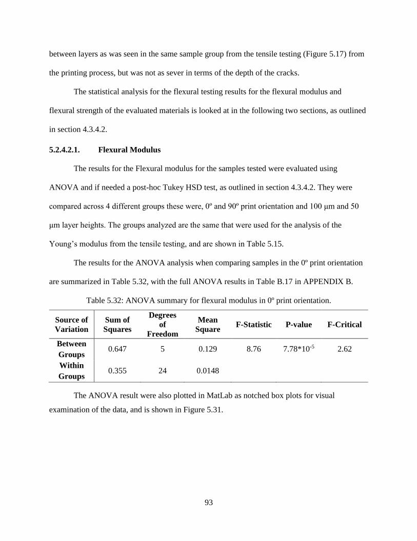
93

between layers as was seen in the same sample group from the tensile testing (Figure 5.17) from

the printing process, but was not as sever in terms of the depth of the cracks.

The statistical analysis for the flexural testing results for the flexural modulus and

flexural strength of the evaluated materials is looked at in the following two sections, as outlined

in section 4.3.4.2.

5.2.4.2.1. Flexural Modulus

The results for the Flexural modulus for the samples tested were evaluated using

ANOVA and if needed a post-hoc Tukey HSD test, as outlined in section 4.3.4.2. They were

compared across 4 different groups these were, 0º and 90º print orientation and 100 μm and 50

μm layer heights. The groups analyzed are the same that were used for the analysis of the

Young’s modulus from the tensile testing, and are shown in Table 5.15.



Table 5.32: ANOVA summary for flexural modulus in 0º print orientation.

Source of

Variation

Sum of

Squares

Degrees

of

Freedom

Mean


Between

Groups 0.647 5 0.129 8.76 7.78*10-5 2.62

Within

Groups 0.355 24 0.0148



94

Figure 5.31: Box plot of ANOVA results for flexural modulus in 0º print orientation.



at least two of the sample groups tested [50]. From Figure 5.31, a visual determination can be

made to determine which groups differ, and can be seen that there is some separation between

the means of the samples. The summarized results of the Tukey test for the 0º sample groups that

showed significant differences are shown in Table 5.33, with the full Tukey results in


95

Table 5.33: Tukey HSD results for flexural modulus in 0º print orientation.



Tukey HSD

inference

M100-0 vs LP50-0 5.3509 0.010389 p<0.05

LP100-0 vs CF100-0 4.5896 0.0357898 p<0.05

LP100-0 vs CF50-0 5.5862 0.0069875 p<0.01

CF100-0 vs LP50-0 6.7263 0.0010053 p<0.01

M50-0 vs LP50-0 5.9136 0.0039968 p<0.01

LP50-0 vs CF50-0 7.7229 0.0010053 p<0.01

The LP samples had a lower modulus due to the increased compliance of the specimens

from the cracks being present [44]. While the CF50-0 sample did not show any significant

difference when compared to the neat Moai resin samples, the higher median and mean value

when compared to the CF100-0 in the box plot indicates that the smaller layer height is aligning

some fibers. There was also outliers present in both the CF100-0 and CF50-0 samples indicating

that the sample manufacturing process could be improved for better consistency [50].



Table 5.34: ANOVA summary for flexural modulus in 90º print orientation.

Source of

Variation

Sum of

Squares

Degrees

of

Freedom

Mean


Between

Groups 0.326 5 0.0652 4.52 4.82*10-3 2.62

Within

Groups 0.347 24 0.0144



96

Figure 5.32: Box plot of ANOVA results for flexural modulus in 90º print orientation.




made to determine which groups differ, and can be seen that there is some separation between

the means of the samples of the CF100-90. The summarized results of the Tukey test for the 0º



97

Table 5.35: Tukey HSD results for flexural modulus in 90º print orientation.


Statistic

Tukey HSD p-

value

Tukey HSD

Inference

CF100-90 vs M50-90 5.9428 0.0037998 p<0.01

CF100-90 vs CF50-90 5.0608 0.0168014 p<0.05

The Tukey HSD results showed only a difference for the CF100-90 specimen due to their

lower flexural modulus. The flexural modulus would be expected to be similar to that of the

CF100-0 sample, but showed a 13% decrease. This could be due to the inconsistency in the fiber

distribution, or due to some fiber alignment occurring and causing the sample to have a

decreased modulus.



B.

Table 5.36: ANOVA summary for flexural modulus printed at 100 μm layer height.

Source of

Variation

Sum of

Squares

Degrees

of

Freedom

Mean


Between

Groups 0.331 5 0.0661 4.18 7.09*10-3 2.62

Within

Groups 0.379 24 0.0158



98

Figure 5.33: Box plot of ANOVA results for flexural modulus printed at 100 μm layer height.



at least two of the sample groups tested [50]. From Figure 5.33 a visual determination can be

made to determine which groups differ, and that there is some separation between the samples,

but most of the notches overlap. This is impart due to the lager standard of deviation, and

therefore large spread in data, of the CF100-90 samples. The summarized results of the Tukey

test for the 100 μm layer height sample groups that showed significant differences are shown in

Table 5.37, with the full Tukey results in APPENDIX B, Table B.22.

99

Table 5.37: Tukey HSD results for flexural modulus printed at 100 μm layer height.



Tukey HSD

inference

LP100-0 vs CF100-0 4.4395 0.0451671 p<0.05

CF100-0 vs CF100-90 5.0123 0.0181893 p<0.05

The flexural modulus of CF100-0 showed higher stiffness than the CF100-90 although it

would be expected that they would show close to the same value, due to the 100 μm layer height.

This could be due to the fiber volume gradient being more pronounced in the 90º printed samples

when compared to the 0º printed samples. The 90º printed samples would have a gradient that

runs long ways across the span from support to support, whereas the 0º printed samples would

have a gradient going perpendicular to this, allowing the fiber to have more of an effect increase

the stiffness.



B.

Table 5.38: ANOVA summary for flexural modulus printed at 50 μm layer height.

Source of

Variation

Sum of

Squares

Degrees

of

Freedom

Mean


Between

Groups 0.596 5 0.119 5.73 1.29*10-3 2.62

Within

Groups 0.499 24 0.0208



100

Figure 5.34: Box plot of ANOVA results for flexural modulus printed at 50 μm layer height.




made to determine which groups differ. From these box plots it can be seen that there is some

separation between the means of the samples, but most of the notches overlap. The summarized

results of the Tukey test for the 50 μm layer height sample groups that showed significant

differences are shown in Table 5.39, with the full Tukey results in APPENDIX B, Table B.24.

101

Table 5.39: Tukey HSD results for flexural modulus printed at 50 μm layer height.


Statistic

Tukey HSD p-

value

Tukey HSD

Inference

M50-0 vs LP50-0 4.986 0.0189857 p<0.05

LP50-0 vs CF50-0 6.5116 0.0014191 p<0.01

LP50-0 vs M50-90 6.2542 0.0022196 p<0.01

LP50-0 vs CF50-90 5.5193 0.0078275 p<0.01

From the Tukey HSD results the only groups showing significance difference are the

LP50-0 and LP50-90 groups, due to the cracks with in the specimens increasing compliance and

therefore decreasing the modulus [44].

5.2.4.2.2. Flexural Strength

The results for the flexural strength for the samples were evaluated using ANOVA and if

needed a post-hoc Tukey HSD test, as outlined in section 4.3.4.2. The samples were compared

across 4 different groups; 0º and 90º print orientation, and 100 μm and 50 μm layer heights. The

groups analyzed are the same that were used in the statistical analysis for the Young’s modulus

from the tensile testing, and are shown in Table 5.15.



Table 5.40: ANOVA summary for flexural strength in 0º print orientation.

Source of

Variation

Sum of

Squares

Degrees

of

Freedom

Mean


Between

Groups 2191 5 4382 86.2 1.57*10-14 2.62

Within

Groups 1220 24 50.9 - - -



102

Figure 5.35: Box plot of ANOVA results for flexural strength in 0º print orientation.





separation between the samples. The summarized results of the Tukey test for the 0º sample

groups that showed significant differences are shown in Table 5.41, with the full Tukey results in


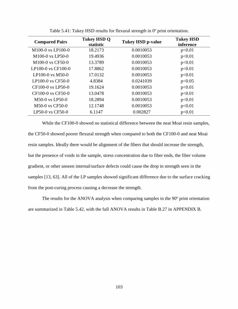
103

Table 5.41: Tukey HSD results for flexural strength in 0º print orientation.



Tukey HSD

inference

M100-0 vs LP100-0 18.2173 0.0010053 p<0.01

M100-0 vs LP50-0 19.4936 0.0010053 p<0.01

M100-0 vs CF50-0 13.3789 0.0010053 p<0.01

LP100-0 vs CF100-0 17.8862 0.0010053 p<0.01

LP100-0 vs M50-0 17.0132 0.0010053 p<0.01

LP100-0 vs CF50-0 4.8384 0.0241039 p<0.05

CF100-0 vs LP50-0 19.1624 0.0010053 p<0.01

CF100-0 vs CF50-0 13.0478 0.0010053 p<0.01

M50-0 vs LP50-0 18.2894 0.0010053 p<0.01

M50-0 vs CF50-0 12.1748 0.0010053 p<0.01

LP50-0 vs CF50-0 6.1147 0.002827 p<0.01

While the CF100-0 showed no statistical difference between the neat Moai resin samples,

the CF50-0 showed poorer flexural strength when compared to both the CF100-0 and neat Moai

resin samples. Ideally there would be alignment of the fibers that should increase the strength,

but the presence of voids in the sample, stress concentration due to fiber ends, the fiber volume

gradient, or other unseen internal/surface defects could cause the drop in strength seen in the

samples [13, 63]. All of the LP samples showed significant difference due to the surface cracking

from the post-curing process causing a decrease the strength.



104

Table 5.42: ANOVA summary for flexural strength in 90º print orientation.

Source of

Variation

Sum of

Squares

Degrees

of

Freedom

Mean


Between

Groups 42490 5 8497 362 8.89*10-22 2.62

Within

Groups 563 24 23.5 - - -



Figure 5.36: Box plot of ANOVA results for flexural strength in 90º print orientation.


for the 95% confidence level chosen. This indicates that there is significant difference between

105

the sample groups tested [50]. From Figure 5.36, many of the samples do not overlap indicating

differences between the groups. The summarized results of the Tukey test for the 90º sample

groups that showed significant differences are shown in Table 5.43, with the full Tukey results in


Table 5.43: Tukey HSD results for flexural strength in 90º print orientation.


Statistic

Tukey HSD p-

value

Tukey HSD

Inference

M100-90 vs LP100-90 37.6398 0.0010053 p<0.01

M100-90 vs CF100-90 13.8998 0.0010053 p<0.01

M100-90 vs LP50-90 38.3222 0.0010053 p<0.01

M100-90 vs CF50-90 35.43 0.0010053 p<0.01

LP100-90 vs CF100-90 23.74 0.0010053 p<0.01

LP100-90 vs M50-90 39.7961 0.0010053 p<0.01

CF100-90 vs M50-90 16.056 0.0010053 p<0.01

CF100-90 vs LP50-90 24.4225 0.0010053 p<0.01

CF100-90 vs CF50-90 21.5302 0.0010053 p<0.01

M50-90 vs LP50-90 40.4785 0.0010053 p<0.01

M50-90 vs CF50-90 37.5862 0.0010053 p<0.01

For the samples printed in the 90º orientation, there is a large amount of difference

between the groups, impart due to the cracks that were present in the LP100-90, LP50-90, and

the CF50-0 decreasing the flexural strength results. The CF100-90 and CF50-90 again showed

weaker flexural strength then the neat Moai resin samples.



B.

106

Table 5.44: ANOVA summary for flexural strength printed at 100 μm layer height.

Source of

Variation

Sum of

Squares

Degrees

of

Freedom

Mean


Between

Groups 28450 5 5690 132 1.19*10-16 2.62

Within

Groups 1030 24 43.1 - - -

The ANOVA result were also plotted in MatLab as box plots for visual examination of

the data, and is shown in Figure 5.37.

Figure 5.37: Box plot of ANOVA results for flexural strength printed at 100 μm layer height.

107





separation between a few of the samples. The summarized results of the Tukey test for the 100

μm layer height sample groups that showed significant differences are shown in Table 5.45, with

the full Tukey results in APPENDIX B, Table B.30.

Table 5.45: Tukey HSD results for flexural strength printed at 100 μm layer height.



Tukey HSD

inference

M100-0 vs LP100-0 19.7968 0.0010053 p<0.01

M100-0 vs LP100-90 24.3289 0.0010053 p<0.01

M100-0 vs CF100-90 6.8084 0.0010053 p<0.01

LP100-0 vs CF100-0 19.437 0.0010053 p<0.01

LP100-0 vs M100-90 23.2466 0.0010053 p<0.01

LP100-0 vs LP100-90 4.5321 0.0391507 p<0.05

LP100-0 vs CF100-90 12.9884 0.0010053 p<0.01

CF100-0 vs LP100-90 23.9691 0.0010053 p<0.01

CF100-0 vs CF100-90 6.4485 0.0015818 p<0.01

M100-90 vs LP100-90 27.7788 0.0010053 p<0.01

M100-90 vs CF100-90 10.2582 0.0010053 p<0.01

LP100-90 vs CF100-90 17.5205 0.0010053 p<0.01

While the lower strength of the LP samples is causing a lot of the difference seen in the

analysis, the CF100-0 was found to not be statistically different from the M100-0 sample, but

again the lower result of the CF100-90 is seen. When comparing the M100-0 and M100-90

results the higher strength seen in the M100-90 is due to the surface defects not being present in

the tested area of the specimen. This is the same as was seen with the tensile specimens in

section 5.2.4.1.

108



B.

Table 5.46: ANOVA summary for flexural strength at 50 μm layer height.

Source of

Variation

Sum of

Squares

Degrees

of

Freedom

Mean


Between

Groups 32950 5 6590 211 5.18*10-19 2.62

Within

Groups 750 24 31.2 - - -



109

Figure 5.38: Box plot of ANOVA results for flexural strength printed at 50 μm layer height.



the sample groups compared [50]. From Figure 5.38, there is separation between most of the

samples. The summarized results of the Tukey test for the 50 μm layer height sample groups that

showed significant differences are shown in Table 5.47, with the full Tukey results in


110

Table 5.47: Tukey HSD results for flexural strength printed at 50 μm layer height.


Statistic

Tukey HSD p-

value

Tukey HSD

Inference

M50-0 vs LP50-0 23.3327 0.0010053 p<0.01

M50-0 vs CF50-0 15.532 0.0010053 p<0.01

M50-0 vs M50-90 7.4543 0.0010053 p<0.01

M50-0 vs LP50-90 27.6164 0.0010053 p<0.01

M50-0 vs CF50-90 25.1105 0.0010053 p<0.01

LP50-0 vs CF50-0 7.8008 0.0010053 p<0.01

LP50-0 vs M50-90 30.7871 0.0010053 p<0.01

CF50-0 vs M50-90 22.9863 0.0010053 p<0.01

CF50-0 vs LP50-90 12.0844 0.0010053 p<0.01

CF50-0 vs CF50-90 9.5786 0.0010053 p<0.01

M50-90 vs LP50-90 35.0707 0.0010053 p<0.01

M50-0 vs LP50-0 32.5649 0.0010053 p<0.01

Again the M50-90 sample had higher strength than the M50-0, due to the surface defects

left behind on the M50-0 from the support material during printing. While the CF50-0 did have

higher strength then the CF50-90, as would be expected if the fiber alignment was being

influenced by the decreasing of the layer high, the cracks present from the printing process in the

CF50-90 would be the main cause in the differences of the strengths. The LP samples again

showed poor flexural strength due to the presence of surface cracks from the post-curing process.

5.2.4.3. Fracture Testing



section 4.2.1. Fracture samples were manufactured and prepared as per sections 4.2.2, 4.2.3, and

4.3.5.1. The flexural testing was carried out as described in section 4.3.5.1, with the exception

the test numbers 4,8,12, and 16 from Table 4.12 were left out. The test numbers omitted

represent the samples made with carbon fiber and no thermal initiator which was shown as

ineffective in section 5.1.1. The settings changed from default for the Moai printer are the same

that were used in Table 5.5 unless otherwise stated. As in section 5.2.4.1, a thin layer of neat

111

Moai resin to the print bed before starting the print aided in keeping the part fixed to the bed

during the printing process. With the same naming convention used for the samples as shown in

Table 5.12.

From ASTM D5045 [54] the procedure to find the fracture toughness from the load-

displacement curves involves verifying that plane-strain testing conditions were met. To verify

this a conditional fracture toughness (KQ) is first found using Equation 5.1,

𝐾𝑄 = (𝑃𝑚𝑎𝑥

𝐵𝑊1/2) 𝑓(𝑥), (5.1)

where,

𝑓(𝑥) = 6𝑥1/2 [1.99−𝑥(1−𝑥)(2.15−3.93𝑥+2.7𝑥3)]

(1+2𝑥)(1−𝑥)3/2 , and 𝑥 = 𝑎/𝑊, (5.2)

where, B is thickness, W is width, and Pmax is the peak load from the load-displacement curve.

Once KQ is found it has to be verified that the plastic zone is small enough for small scale

yielding to be valid. This is checked by using the following inequality, Equation 5.3.

𝐵, 𝑎, (𝑊 − 𝑎) > 2.5 (

𝐾𝑄𝜎𝑦

⁄ )2

if true, 𝐾𝑄 = 𝐾𝐼𝐶 (5.3)

This inequality was found to be true for all specimens tested, and indicated that the

specimen size could be reduced for future testing. This would aid in decreasing print times need

to prepare the samples.

The fracture toughness was found as specified in ASTM D5045 section A1.4, and the

results are shown for the samples printed in the 0º orientation in Figure 5.39, for the samples

printed in the 90º orientation in Figure 5.40, and are summarized in Table 5.48 [54].

112

Figure 5.39: Fracture toughness for 0º print orientation.

Figure 5.40: Fracture toughness for 90º print orientation.

113

Table 5.48: Summarized fracture testing results.

Sample Layer Height

(µm)

Print

Orientation

Fiber

Volume

(%)

Fracture

Toughness

𝐊𝐈𝐂 (𝐌𝐏𝐚√𝐦)

M100-0 100 0° 0 0.627 ± 0.126

M100-90 100 90º 0 0.688 ± 0.057

M50-0 50 0° 0 0.654 ± 0.162

M50-90 50 90º 0 0.570 ± 0.078

LP100-0 100 0° 0 0.580 ± 0.182

LP100-90 100 90º 0 0.656 ± 0.116

LP50-0 50 0° 0 0.565 ± 0.083

LP50-90 50 90º 0 0.574 ± 0.133

CF100-0 100 0° 5 0.726 ± 0.146

CF100-90 100 90º 5 0.577 ± 0.065

CF50-0 50 0° 5 0.573 ± 0.045

CF50-90 50 90º 5 0.568 ± 0.056

From the fracture testing carried out on the neat Moai resin, it can be observed that while

the print orientation does not have an effect on the fracture toughness of the material, but the

smaller 50 μm layer height does exhibit a decrease in 90º print orientation. From the specimens

themselves, shown in Figure 5.41, it can be seen that the fracture is consistent with a mode Ⅰ

fracture regardless of the print orientation [44].

Figure 5.41: Fracture testing specimens.

The fracture toughness of the CF100-0 shows a 15.8% increase over the M00-0, but for

all the other CF samples the results showed the same or lower fracture toughness. When

114

comparing the CF100-0 and CF100-90 the larger difference seen could be due to partial

alignment of fibers parallel to the crack direction. While the LP samples showed the same

surface cracking as seen previously in the tensile and flexural testing it does not appear to have

had as large of an effect on the fracture toughness as it did on other material properties.

The incorporation of short-fibers can increase the fracture toughness by changing the

failure modes associated with crack growth which can include fiber pull-out, bridging, failure,

fiber/matrix debonding, and matrix cracking [44]. Ideally the change in the failure modes require

more energy for crack initiation and propagation therefore increasing the fracture toughness, and

would result in the composite having a higher fracture toughness then the matrix material [44].

From the tensile testing (section 5.2.4.1) it was shown that the composite had weak interfacial

strength. The weak interfacial strength can cause the composite to have a weaker fracture

toughness than the neat matrix, and the short-fiber lengths used in the CF samples can limit the

energy need for fiber pull-out and crack bridging [44]. The incorporation of longer fiber lengths

and/or increasing the fiber volume could help to increase the fracture toughness of the material in

any future research [65].

Appling the statistical methods outlined in section 4.3.5.2 the results of the fracture

toughness can be compared across the different layer heights and print orientations to help

identify any trends within the data.

The results for the ANOVA analysis when comparing the fracture toughness of samples

in the 0º print orientation are summarized in Table 5.49, with the full ANOVA results in Table

B.33 in APPENDIX B.

115

Table 5.49: ANOVA summary for fracture toughness in the 0º print orientation.

Source of

Variation

Sum of

Squares

Degrees

of

Freedom

Mean


Between

Groups 0.0579 5 0.0116 0.6567 0.6627 3.1059

Within

Groups 0.2116 12 0.0176 - - -



Figure 5.42: Box plot of ANOVA results for fracture toughness in the 0º print orientation.



116



samples within the 95% confidence level, represented by the ends of the notches. This is in part

due to the large deviation with some of the tested samples. If this deviation could be corrected

for more consistent samples then the CF100-0 could possibly be statistical different than the

other samples tested. This is seen in the box plots median value (0.757 K1C) for the CF100-0

being higher than its mean value (0.726 K1C) and that of the M100-0 sample. This could

indicate that the potential for improvement in the fracture toughness is possible. For

completeness, the Tukey HSD test was still carried out with none of the results indicating any

significant differences. The results of the Tukey test for the 0º sample groups can be found in



in the 90º print orientation are summarized in Table 5.50, with the full ANOVA results in Table

B.35 in APPENDIX B.

Table 5.50: ANOVA summary for fracture toughness in the 90º print orientation.

Source of

Variation

Sum of

Squares

Degrees

of

Freedom

Mean


Between

Groups 0.0418 5 0.0084 1.05 0.435 3.11

Within

Groups 0.0957 12 0.0080 - - -



117

Figure 5.43: Box plot of ANOVA results for fracture toughness in the 90º print orientation.





samples within the 95% confidence level, represented by the ends of the notches. This is again

due to the large deviation with some of the tested samples. It can also be seen that the 100 μm

layer height samples have a higher median value than the 50 μm layer height samples, but

without smaller deviation of the samples conclusions that can be drawn are limited. For

completeness, the Tukey HSD test was still carried out with none of the results indicating any

118

significant differences. The results of the Tukey test for the 90º sample groups can be found in



printed at a 100 μm layer height are summarized in Table 5.51, with the full ANOVA results in

Table B.37 in APPENDIX B.

Table 5.51: ANOVA summary for fracture toughness of 100 μm layer height.

Source of

Variation

Sum of

Squares

Degrees of

Freedom

Mean


Between

Groups 0.0533 5 0.0107 0.6972 0.6358 3.10588

Within

Groups 0.1834 12 0.0153 - - -



119

Figure 5.44: Box plot of ANOVA results for fracture toughness of 100 μm layer height.





samples within the 95% confidence level, represented by the ends of the notches. These results

demonstrate that the print orientation is not having an effect on the fracture toughness of the

samples. For completeness, the Tukey HSD test was still carried out with none of the results

indicating any significant differences. The results of the Tukey test for the 90º sample groups can

be found in APPENDIX B, Table B.38.

120


printed at a 50 μm layer height are summarized in Table 5.52, with the full ANOVA results in

Table B.39 in APPENDIX B.

Table 5.52: ANOVA summary for fracture toughness of 50 μm layer height.

Source of

Variation

Sum of

Squares

Degrees of

Freedom

Mean


Between

Groups 0.0176 5 0.0035 0.3416 0.8780 3.10588

Within

Groups 0.1240 12 0.0103 - - -



Figure 5.45: Box plot of ANOVA results for fracture toughness of 50 μm layer height.

121




confirm that the groups do not differ, and it can be seen that the medians of the samples (red line)

in the box plots are similar. For the 50 μm layer height samples the addition of carbon fiber

and/or thermal initiator along with the print orientation had no influence on the fracture

toughness. For completeness, the Tukey HSD test was still carried out with none of the results

indicating any significant differences. The results of the Tukey test for the 90º sample groups can

be found in APPENDIX B, Table B.40.

122

6. CONCLUSIONS AND RECOMMENDATIONS

6.1. Conclusions

The use of carbon fiber as a reinforcement in a short-fiber composite produced using

stereolithography was experimentally investigated through this research. The use of a dual curing

system consisting of a photo initiator for forming the part geometry, and a thermal initiator to

completely cure the part was shown to be an effective method when using carbon fiber to

manufacture composites using SLA printers.

To identify and evaluate the effectiveness of using a dual cure system for the

manufacturing of carbon fiber composites, several thermal initiators were investigated through

DSC, and the solubility and stability of the thermal initiators in the system was explored.

From the solubility testing it was found that several thermal initiators could be

incorporated into the system. The ease of use from a processing stand point, were the thermal

initiators that were liquid at room temperature. This aided in the dispersion and incorporation of

the thermal initiator into the resin. The stability aspect that was evaluated proved to be an

important area, due to some thermal initiators being evaluated that resulted in the system gelling

within a short period of time. This could lead to polymerization during the printing process

causing part failure, and potential damage to the print apparatus. While the Luperox P was stable

during the printing process, it was observed that resin left out for a week at ambient temperatures

would began to gel. This would only happen to the carbon fiber that had settled to the bottom of

the container, while the remaining resin would still be unreacted. This could have been due to the

thermal initiator undergoing induced decomposition from the increased concentration of carbon

fiber [59]. Other possible thermal initiators to overcome this are discussed in the following

Future Recommendations section.

123

From the DSC results it was determine that the neat Moai resin did not exhibit any curing

due to thermal processing, but with the incorporation of a thermal initiator the resin would cure

both with and without prior UV curing. Luperox P was chosen as the thermal initiator that yield

the best results from the ones evaluated, both from a processing and material properties

perspective.

To determine the effects of the printing process on the manufacturing of short-fiber

composite the void content of the composite, fiber volume consistency, and resin viscosity were

evaluated.

The void content of the samples produce showed to differ with the layer height of the

sample printed. For a layer height of 100 μm a void content of 1.3% was found, while a layer

height of 50 μm had a void content of 0.7%. The differences seen in the void content could have

originated for two different sources. From when part is being printed, the layer that is currently

being cured during the print has a reduction in the volume when going from the liquid state to the

solid state, and creating free space. The smaller layer height would have less of a reduction due

to less material changing phase, and therefore less free space. This would allow for the resin to

recoat the vat easier, and therefore reducing the chance that voids could become trapped in the

resin. The larger layer height would have more unreacted resin after the photo polymerization

process, and while going through the thermal post curing process produce more gas byproducts

from the reaction of the thermal initiator and resin, resulting in an increase in the void content

[61].

The addition of the carbon fiber to the Moai resin was shown to increase the viscosity of

the resin by 57%, but with the addition of the liquid thermal initiator (Luperox P) into the system

it was lowered to only a 26% increase. The resin also showed some shear thinning behavior that

124

could have an influence on the fiber orientation with the part, and the ability for the fiber to stay

suspended within the resin. To overcome this increase in resin viscosity, printing parameters

where changed that increased the distance that the vat tilted down during the peel step to allow

for more time and to increase resin flow over the processing area. The fiber volume consistency

was found to not vary with time, but be due to the fiber dispersed in the resin within the

immediate area of the part becoming depleted. To improve the fiber volume consistency a

method of mixing the resin during the printing processes should be used in future research.

To evaluated the effects of the carbon fiber on the material properties the composite was

evaluated by tensile, flexural, and fracture testing. While comparing what effects layer height

and print orientation have on the material properties of the produced short-fiber composite.

From the tensile testing results, the carbon fiber samples showed an increase in Young’s

modulus of 21% for a 100 μm layer height, and a 27% for a 50 μm layer height. The change in

the modulus due to the lower layer high is due to the fibers being aligned in the loading direction

with in the sample. This demonstrates that manipulating a part’s properties based off of fiber

length and layer height could be possible. This increase was less than what was predicted by

theoretical models. The lower modulus was thought to be due to large distribution of fiber

lengths and poor interfacial properties between the carbon fiber and matrix. These defects also

lead to the carbon fiber samples having a lower tensile strength then the neat Moai resin samples.

With improvements in these areas the tensile properties of the composite could be further

improved.

The flexural strength, flexural modulus, and fracture toughness showed no noticeable

gains in material properties from the use of the carbon fiber reinforcement. For the flexural

testing this is thought to be due because of the low fiber volume (5%) and high fiber volume

125

inconsistency of the samples. The low fiber volume (5%) and short fiber lengths (76 μm) of the

fracture samples resulted in no improvements in fracture toughness, but also did not cause any

decrease in the fracture toughness.

While factors such as interfacial strength, fiber length distribution and volume

consistency, and low fiber volume content lowered the effectiveness of the carbon fiber as a

reinforcement the main limiting factor is the fiber length itself. The average fiber length used

was 76 μm. This is much shorter than the critical fiber length that was found to be 433 μm for the

system. While it would be possible to incorporate fibers of this length into the resin and print

parts, they could not have isotropic properties due to forced alignment of the layer height. The

effects of fibers folding over within the layers could also affect the ability for the part to print

successfully. This could be by limiting the amount of matrix material available to keep the layers

attached to one and another. To avoid this it would require a layer height at least as larger as the

fiber length itself. This is outside of the capabilities of even industrial grade SLA printers, that

typical print at around 200 μm on the top end of layer height [5]. The incorporation of carbon

fiber and the subsequent shadowing of the photo initiator from the UV source would even further

limit the depth of cure that could be achieved. So while it might not be feasible to use fiber with

a length of 433 μm, increasing the fiber length and tightening the fiber length distribution would

aid in increasing the material properties for the samples studied in this research.

The research does show that the use of a dual cure resin system could be used for the

additive manufacturing of carbon fiber composites, and can provide a good starting point for the

continuation of this area of research.

126

6.2. Future Recommendations

To aid in the continuation of the research carried out in this study, the following section

provides recommendations in both the areas of processing and material improvements. Looking

specifically and the type of thermal initiators, fibers, and apparatus used.

For this research all of the thermal initiators looked at for their possible use in the dual

cure system were organic peroxides There is another class of thermal initiators that are

commonly used for free radical polymerization, known as aliphatic azo compounds (azo). The

azo initiators are not as effected by fillers, and do not undergo radical induced decomposition

[66]. This could prove useful for the long-term stability of the resins used for manufacturing

short-fiber composites via SLA.

The carbon fiber used in this research was sized for an epoxy matrix. With the use of a

carbon fiber sized for use with a urethane or vinyl ester matrix, the interfacial properties might

be increased, and therefore the material properties of the composite. The other method of

approach would be to use a different resin for the matrix material. There are SLA resins that are

commercially available that are labeled as epoxy resins. While these are not true epoxies, they do

contain bisphenol A in the polymer chain, and could prove to bond better to the carbon fiber

sized for an epoxy matrix. If these types of resin are to be used with the SLA printer used in this

research, a different vat bed/coating would have to be used. The epoxy SLA resins react with the

silicon layer used in the vats, causing the parts to stick and subsequently fail.

During the process of conducting the research for this study, there was one factor within

the printing process that seemed to limit the composites that could be produced, and this was the

use of a bottom-up SLA style printer. This is mainly due to the peel step that is used to separate

the layer from the vat. It was seen in the cracks that were produced when printing at the 50 μm

127

layer height causing failure, and why any attempts to print parts at higher fiber volumes (7.5%

and 10%) resulted in print failure. By switching to a top-down style printer this peel step would

be removed, and there would be an added benefit from not have to use as much support material.

This is because it would only be need to keep the part in place, not support it from the forces

generated in the peel step.

The use of a top-down style printer could also allow for the easy incorporation of a

pump/mixing unit to help maintain fiber volume consistency. While this was tried for the Moai

printer the main limitation was the lack of space for equipment of the necessary size to be

incorporated, due to the limited free space available in the vat with the print bed present. Because

of the large vat size need for the top-down style printer adding a pump to the tank, along with an

angled bottom, should allow for mixing of the resin to maintain a constant fiber distribution

during the printing process. One issue that would need to be addressed would be for the printing

of parts that have random fiber orientation, and therefore isotropic properties. During the printing

process for top-down style machines, a recoat blade moves across the top of the tank to smooth

out the resin for the printing of the next layer. This has been shown by Cheah C. et al. to produce

near unidirectional composites and could limit the applications of the parts produced [32]. This

might be overcome by not including the recoat blade, but adjusting the raising and lowering

settings for the build platform. This would allow for some settling to occur, but would increase

the print time of the parts.

128

REFERENCES

[1] Hull, C. W., 1986, "Apparatus for production of three-dimensional objects by

stereolithography," U.S. Patent 4575330A.

[2] Wang, X., Jiang, M., Zhou, Z., Gou, J., and Hui, D. "3D printing of polymer matrix

composites: A review and prospective." Composites Part B: Engineering Vol. 110

(2017): pp. 442-458.

[3] Karalekas, D., and Antoniou, K. "Composite rapid prototyping: overcoming the

drawback of poor mechanical properties." Journal of Materials Processing Technology

Vol. 153-154 (2004): pp. 526-530.

[4] Parandoush, P., and Lin, D. "A review on additive manufacturing of polymer-fiber

composites." Composite Structures Vol. 182 (2017): pp. 36-53.

[5] Jacobs, P. F., Rapid Prototyping & Manufacturing: Fundamentals of Stereolithography,

Society of Manufacturing Engineers, (1992)

[6] Tumbleston, J. R., Shirvanyants, D., Ermoshkin, N., Janusziewicz, R., Johnson, A. R.,

Kelly, D., Chen, K., Pinschmidt, R., Rolland, J. P., and Ermoshkin, A. "Continuous liquid

interface production of 3D objects." Science (2015): DOI 10.1126/science.aaa2397

[7] "DruckWege Resin Technical Datasheet," https://druckwege.de/wp-

content/uploads/2018/07/Technical-Datasheet_TypD_English_v6.pdf. Accessed 2018

[8] "FLGPCL03 Clear Resin Technical Datasheet,"

https://formlabs.com/media/upload/Clear-DataSheet.pdf. Accessed 2018

[9] "Moai Clear Resin Technical Datasheet." ." http://wiki.peopoly.net/doku.php?id=moai-

resin. Accessed 2018

[10] Zguris, Z. "How mechanical properties of stereolithography 3D prints are affected by UV

curing." Formlabs, Inc., Somerville, MA, 2017.

[11] Stansbury, J. W., and Idacavage, M. J. "3D printing with polymers: Challenges among

expanding options and opportunities." Dental Materials Vol. 32 No. 1 (2016): pp. 54-64.

[12] Ogale, A. A., and Renault, T. "3-D Photolithography for Composite Development:

Discontinuous Reinforcements," SAMPE Quarterly Vol. 5, No. 6 (1991): pp. 28-38

[13] Agarwal, B. D., Broutman, L. J., and Chandrashekhara, K. Analysis and Performance of

Fiber Composites, John Wiley & Sons, New York (2017).

[14] Taya, M., and Arsenault, R. J. "A comparison between a shear lag type model and an

eshelby type model in predicting the mechanical properties of a short fiber composite,"

Scripta Metallurgica Vol. 21 No. 3 (1987): pp. 349-354.

129

[15] Mortazavian, S., and Fatemi, A. "Effects of fiber orientation and anisotropy on tensile

strength and elastic modulus of short fiber reinforced polymer composites," Composites

Part B: Engineering, Vol. 72 (2015): pp. 116-129.

[16] Papthanasiou, T. D., and Guell, D. C. Flow-induced alignment in composite materials,

Elsevier (1997)

[17] Zainudin, E. S., Sapuan, S. M., Sulaiman, S., and Ahmad, M. "Fiber orientation of short

fiber reinforced injection molded thermoplastic composites: A review," Journal of

Injection Molding Technology, Vol. 6 No. 1 (2002): pp. 1.

[18] Tucker Iii, C. L., and Liang, E. "Stiffness predictions for unidirectional short-fiber

composites: Review and evaluation," Composites Science and Technology, Vol. 59 No. 5

(199): pp. 655-671.

[19] Altan, M. C. "A Review of Fiber-Reinforced Injection Molding: Flow Kinematics and

Particle Orientation," Journal of Thermoplastic Composite Materials, Vol. 3 No. 4

(1990): pp. 275-313.

[20] Vincent, M., Giroud, T., Clarke, A., and Eberhardt, C. "Description and modeling of fiber

orientation in injection molding of fiber reinforced thermoplastics," Polymer, Vol. 46 No.

17 (2005): pp. 6719-6725.

[21] Chung, D. H., and Kwon, T. H. "Fiber orientation in the processing of polymer

composites," Korea-Australia Rheology Journal, Vol. 14 No. 4 (2002): pp. 175-188.

[22] Goh, G. D., Dikshit, V., Nagalingam, A. P., Goh, G. L., Agarwala, S., Sing, S. L., Wei,

J., and Yeong, W. Y. "Characterization of mechanical properties and fracture mode of

additively manufactured carbon fiber and glass fiber reinforced thermoplastics."

Materials & Design Vol. 137 (2018): pp. 79-89.

[23] Ferreira, R. T. L., Amatte, I. C., Dutra, T. A., and Bürger, D. "Experimental

characterization and micrography of 3D printed PLA and PLA reinforced with short

carbon fibers." Composites Part B: Engineering, Vol. 124 (2017): pp. 88-100.

[24] Ning, F., Cong, W., Qiu, J., Wei, J., and Wang, S. "Additive manufacturing of carbon

fiber reinforced thermoplastic composites using fused deposition modeling." Composites

Part B: Engineering Vol. 80 (2015): pp. 369-378.

[25] Hector Sandoval, J., and Wicker, R. B. "Functionalizing stereolithography resins: effects

of dispersed multi‐walled carbon nanotubes on physical properties." Rapid Prototyping

Journal Vol. 12 No. 5 (2006): pp. 292-303.

[26] Yang, Z., Wu, G., Wang, S., Xu, M., and Feng, X. "Dynamic postpolymerization of 3D-

printed photopolymer nanocomposites: Effect of cellulose nanocrystal and postcure

temperature." Journal of Polymer Science Part B: Polymer Physics Vol. 56 No. 12

(2018): pp. 935-946.

130

[27] Feng, X., Yang, Z., Chmely, S., Wang, Q., Wang, S., and Xie, Y. "Lignin-coated

cellulose nanocrystal filled methacrylate composites prepared via 3D stereolithography

printing: Mechanical reinforcement and thermal stabilization." Carbohydrate Polymers

Vol. 169 (2017): pp. 272-281.

[28] Tekinalp, H. L., Kunc, V., Velez-Garcia, G. M., Duty, C. E., Love, L. J., Naskar, A. K.,

Blue, C. A., and Ozcan, S. "Highly oriented carbon fiber–polymer composites via

additive manufacturing." Composites Science and Technology Vol. 105 (2014): pp. 144-

150.

[29] Thomas, H., David, B. P., Guido, T., and Hans, N. H. "State-of-the-art of fiber-reinforced

polymers in additive manufacturing technologies." Journal of Reinforced Plastics and

Composites Vol. 36 No. 15 (2017): pp. 1061-1073.

[30] Gupta, A., and Ogale, A. A. "Dual curing of carbon fiber reinforced photoresins for rapid

prototyping." Polymer Composites Vol. 23 No. 6 (2002): pp. 1162-1170.

[31] Taormina, G., Sciancalepore, C., Bondioli, F., and Messori, M. "Special resins for

stereolithography: In situ generation of silver nanoparticles." Polymers Vol. 10

No.2:(2018) pp. 212.

[32] Cheah, C. M., Nee, A. Y. C., Fuh, J. Y. H., and Lu, L., "Mechanical characteristics of

fiber‐filled photo‐polymer used in stereolithography." Rapid Prototyping Journal Vol. 5

No. 3 (199): pp. 112-119.

[33] Grasso, M., Martorelli, M., Lanzotti, A., and Staiano, G. "The impact of process

parameters on mechanical properties of parts fabricated in PLA with an open-source 3-D

printer," Rapid Prototyping Journal, Vol. 21 No. 5 (2015): pp. 604-617.

[34] L. Dunn, M., Suwito, W., and Cunningham, S. "Fracture Initiation at Sharp Notches:

Correlation Using Critical Stress Intensities." International Journal of Solids and

Structures Vol. 34 No. 29 (1997): pp 3873-3883

[35] Lerch, B. A., Thesken, J. C., and Bunnell, C. T. "Polymethylmethacrylate (PMMA)

material test results for the capillary flow experiments (CFE)."Technical Report No.

NASA/TM‐2007‐214835 NASA STI Program, Cleveland, OH. 2007

[36] Huang Donald, D. "The application of fracture mechanics to short fiber composites."

Polymer Composites Vol. 16 No. 1 (2004): pp. 10-16.

[37] Mower, T. M., and Li, V. C. "Fracture characterization of random short fiber reinforced

thermoset resin composites," Engineering Fracture Mechanics, Vol. 26 No. 4 (1987): pp.

593-603.

[38] Fitzer, E. "Pan-based carbon fibers—present state and trend of the technology from the

viewpoint of possibilities and limits to influence and to control the fiber properties by the

process parameters," Carbon, Vol. 27 No. 5 (1989) pp. 621-645.

131

[39] Yao, S.-S., Jin, F.-L., Rhee, K. Y., Hui, D., and Park, S.-J. "Recent advances in carbon-

fiber-reinforced thermoplastic composites: A review." Composites Part B: Engineering

Vol. 142 (2018): pp. 241-250.

[40] Maradur, S. P., Kim, C. H., Kim, S. Y., Kim, B.-H., Kim, W. C., and Yang, K. S.

"Preparation of carbon fibers from a lignin copolymer with polyacrylonitrile." Synthetic

Metals Vol. 162 No.5 (2012): pp. 453-459.

[41] Chand, S. "Review Carbon fibers for composites." Journal of Materials Science Vol. 35

No. 6(2000) pp. 1303-1313.

[42] "Toray T-700S Technical Datasheet."

https://www.toraycma.com/file_viewer.php?id=4459 Accessed 2018

[43] "Carbiso MF SM45R-100 Technical Datasheet."

http://www.elgcf.com/assets/datasheets/Carbiso-MF-TDS.pdf Accessed 2018

[44] Anderson, T. L. Fracture Mechanics: Fundamentals and Applications, CRC press, Boca

Rarton, FL, (2005)

[45] ASTM E2160-04 Standard Test Method for Heat of Reaction of Thermally Reactive

Materials by Differential Scanning Calorimetry, ASTM International, West

Conshohocken, PA, 2018

[46] Instruments, TA, AR-G2/AR 2000ex Operator's Manual, New Castle, DE. (2010)

[47] Shenoy, A. V. Rheology of filled polymer systems, Springer Science & Business Media.

(2013)

[48] ASTM D638-14 Standard Test Method for Tensile Properties of Plastics, ASTM

International, West Conshohocken, PA, 2014

[49] ASTM D3039/D3039M-17 Standard Test Method for Tensile Properties of Polymer

Matrix Composite Materials, ASTM International, West Conshohocken, PA, 2017

[50] Levine, D. M., Ramsey, P. P., and Smidt, R. K. Applied statistics for engineers and

scientists: using Microsoft Excel and Minitab, Prentice Hall, Upper Saddle River, (2001).

[51] Devore, J. L. Probability and Statistics for Engineering and the Sciences, Cengage

learning. (2011)

[52] Tukey, J. W. "Comparing Individual Means in the Analysis of Variance," Biometrics,

Vol. 5 No. 2 (1949): pp. 99-114.

[53] ASTM D790-17 Standard Test Methods for Flexural Properties of Unreinforced and

Reinforced Plastics and Electrical Insulating Materials, ASTM International, West

Conshohocken, PA, 2017

132

[54] ASTM D5045-14 Standard Test Methods for Plane-Strain Fracture Toughness and Strain

Energy Release Rate of Plastic Materials, ASTM International, West Conshohocken, PA,

2014

[55] ASTM E399-17 Standard Test Method for Linear-Elastic Plane-Strain Fracture

Toughness KIc of Metallic Materials, ASTM International, West Conshohocken, PA,

2017

[56] ASTM D3171-15 Standard Test Methods for Constituent Content of Composite

Materials, ASTM International, West Conshohocken, PA, 2015

[57] ASTM D792-13 Standard Test Methods for Density and Specific Gravity (Relative

Density) of Plastics by Displacement, ASTM International, West Conshohocken, PA,

2013

[58] Zhang, H., Zhang, Z., and Breidt, C. "Comparison of short carbon fibre surface

treatments on epoxy composites: I. Enhancement of the mechanical properties,"

Composites Science and Technology Vol. 64 No. 13 (2004): pp. 2021-2029.

[59] Dixon, K. W. "Decomposition rates of organic free radical initiators," Polymer handbook

Vol .4 (1999).

[60] Purslow, D. "Matrix fractography of fibre-reinforced epoxy composites," Composites,

Vol. 17 No. 4 (1986): pp. 289-303.

[61] Masere, J., Chekanov, Y., Warren, J. R., Stewart, F. D., Al‐Kaysi, R., Rasmussen, J. K.,

and Pojman, J. A. "Gas‐free initiators for high‐temperature free‐radical polymerization,"

Journal of Polymer Science Part A: Polymer Chemistry, Vol. 38 No. 21 (2000): pp.

3984-3990.

[62] Braga, R. R., Ballester, R. Y., and Ferracane, J. L. "Factors involved in the development

of polymerization shrinkage stress in resin-composites: A systematic review," Dental

Materials, Vol. 21 No. 10 (2005): pp. 962-970.

[63] Chambers, A. R., Earl, J. S., Squires, C. A., and Suhot, M. A. "The effect of voids on the

flexural fatigue performance of unidirectional carbon fibre composites developed for

wind turbine applications," International Journal of Fatigue, Vol. 28 No. 10 (2006): pp.

1389-1398.

[64] Parry, T. V., and Wronski, A. S. "Kinking and tensile, compressive and interlaminar

shear failure in carbon-fibre-reinforced plastic beams tested in flexure," Journal of

Materials Science, Vol. 16 No. 2 (1981): pp. 439-450.

[65] Cholake, S. T., Moran, G., Joe, B., Bai, Y., Singh Raman, R. K., Zhao, X. L., Rizkalla,

S., and Bandyopadhyay, S. "Improved Mode I fracture resistance of CFRP composites by

reinforcing epoxy matrix with recycled short milled carbon fibre," Construction and

Building Materials, Vol. 111 (2016): pp. 399-407.

133

[66] Sheppard Chester, S., and Kamath Vasanth, R. "The selection and use of free radical

initiators," Polymer Engineering & Science, Vol. 19 No. 9 (2004) pp. 597-606.

134

APPENDIX A. EXPERIMENTAL DATA

Figure A.1: DSC curves for Moai resin.

Figure A.2: DSC curves for Luperox P.

135

Figure A.3: DSC curves for dicumyl peroxide.

Figure A.4: DSC curves for cumene hydroperoxide.

136

Figure A.5: Moai resin viscosity curve 1 s-1 to 25 s-1.

Figure A.6: Moai resin viscosity curve 1 s-1 to 100 s-1.

137

Figure A.7: Moai resin + Luperox P viscosity curve 1 s-1 to 25 s-1.

Figure A.8: Moai resin + Luperox P viscosity curve 1 s-1 to 100 s-1.

138

Figure A.9: Moai resin + carbon fiber viscosity curve 1 s-1 to 25 s-1.

Figure A.10: Moai resin + carbon fiber viscosity curve 1 s-1 to 100 s-1.

139

Figure A.11: Moai resin + carbon fiber + Luperox P viscosity curve 1 s-1 to 25 s-1.

Figure A.12: Moai resin + carbon fiber + Luperox P viscosity curve 1 s-1 to 100 s-1.

140

Table A.1: Fiber volume consistency for 100 μm layer height.

100 μm Layer Height Top Weight (g) Middle Weight (g) Bottom Weight (g)

Crucible 6.0931 8.0662 7.7678

Before Burn off 6.2136 8.2070 7.9383

After Burn off 6.0994 8.0731 7.7742

Composite Mass 0.1205 0.1408 0.1705

Fiber Mass 0.0063 0.0069 0.0064

Fiber Weight % 5.2282 4.9006 3.7537

Average 5.2445 4.8363 3.5635

Standard Deviation 0.0230 0.0909 0.2689

Table A.2: Fiber volume consistency for 50 μm layer height.

50 μm Layer Height Top Weight (g) Middle Weight (g) Bottom Weight (g)

Crucible 7.7620 8.0613 6.0937

Before Burn off 7.9545 8.2793 6.3391

After Burn off 7.7727 8.0709 6.1032

Composite Mass 0.1925 0.2180 0.2454

Fiber Mass 0.0107 0.0096 0.0095

Fiber Weight % 5.5584 4.4037 3.8712

Average 5.4544 4.4978 3.8813

Standard Deviation 0.1471 0.1331 0.0143

141

Table A.3: Density measurements results.

100 μm Layer Height 5%Vf Carbon Fiber + 0.5 wt.% Luperox P

Sample Dry Weight (g) Wet Weight (g) Density (g/cm3) Submerged Wire

Weight (g)

1 1.2298 0.8488 1.2545 0.5993

2 1.2168 0.8465 1.2550 0.5993

50 μm Layer Height 5%Vf Carbon Fiber + 0.5 wt.% Luperox P


Weight (g)

1 1.2582 0.8545 1.2544 0.5993

2 1.2456 0.8472 1.2485 0.5993

100 μm Layer Height 0.5 wt.% Luperox P


Weight (g)

1 1.1958 0.8459 1.2424 0.6126

2 1.1866 0.8441 1.2424 0.6126

Table A.4: Void content measurement results.

100 μm Layer Height

Sample Crucible

(g)

Before

Burn

off (g)

After

Burn

off (g)

Composite

Mass (g)

Fiber

Mass

(g)

Fiber

Volume

(%)

Matric

Volume

(%)

Void

Content

(%)

1 7.7642 8.9973 7.8417 1.2331 0.0775 4.3646 94.4708 1.1646

2 8.0640 9.2859 8.1527 1.2219 0.0887 5.0411 93.4887 1.4702

50 μm Layer Height

1 6.0954 7.3537 6.1505 1.2583 0.0551 3.0409 96.3922 0.5669

2 7.4096 8.6793 7.4763 1.2697 0.0667 3.6481 95.5109 0.8411

142

Table A.5: Shrinkage due to post-curing M100.

M100 Before Cure After Cure

Cube X

(mm)

Y

(mm)

Z

(mm)

Volume

(mm3)

X

(mm)

Y

(mm)

Z

(mm)

Volume

(mm3)

1 9.83 9.84 10.4 1005.963 9.81 9.8 10.42 1001.758

2 9.86 9.74 10.38 996.8578 9.79 9.68 10.33 978.9452

3 9.79 9.84 10.58 1019.209 9.75 9.8 10.55 1008.053

4 9.74 9.74 10.58 1003.699 9.7 9.69 10.45 982.2269

5 9.74 9.75 10.48 995.2332 9.69 9.71 10.42 980.4168

Table A.6: Shrinkage due to post-curing M50.

M50 Before Cure After Cure

Cube X

(mm)

Y

(mm)

Z

(mm)

Volume

(mm3)

X

(mm)

Y

(mm)

Z

(mm)

Volume

(mm3)

1 9.77 9.88 10.71 1033.811 9.7 9.85 10.74 1026.153

2 9.78 9.87 10.72 1034.787 9.76 9.82 10.73 1028.398

3 9.77 9.75 10.69 1018.303 9.69 9.74 10.75 1014.591

4 9.94 9.88 10.74 1054.745 9.95 9.83 10.7 1046.551

5 9.78 9.77 10.85 1036.724 9.75 9.72 10.76 1019.725

Table A.7: Shrinkage due to post-curing LP100.

LP100 Before Cure After Cure

Cube X

(mm)

Y

(mm)

Z

(mm)

Volume

(mm3)

X

(mm)

Y

(mm)

Z

(mm)

Volume

(mm3)

1 9.8 9.85 10.54 1017.43 9.67 9.73 10.46 984.172

2 9.86 9.87 10.41 1013.08 9.62 9.75 10.31 967.026

3 9.73 9.75 10.44 990.417 9.61 9.62 10.39 960.537

4 9.8 9.75 10.45 998.498 9.66 9.62 10.37 963.676

5 9.86 9.87 10.43 1015.03 9.73 9.75 10.35 981.879

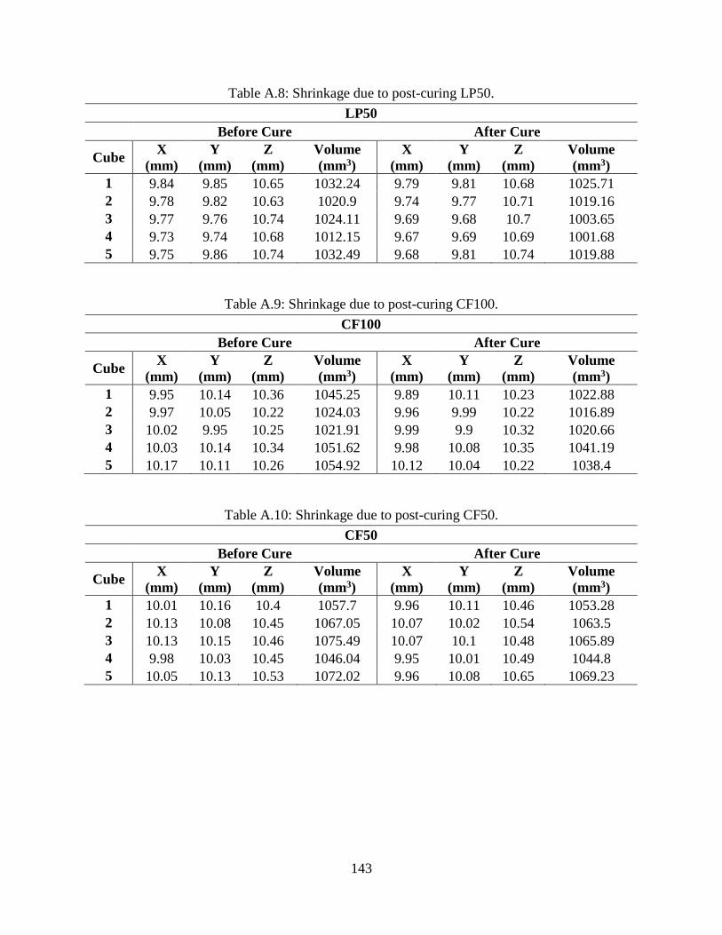
143

Table A.8: Shrinkage due to post-curing LP50.

LP50 Before Cure After Cure

Cube X

(mm)

Y

(mm)

Z

(mm)

Volume

(mm3)

X

(mm)

Y

(mm)

Z

(mm)

Volume

(mm3)

1 9.84 9.85 10.65 1032.24 9.79 9.81 10.68 1025.71

2 9.78 9.82 10.63 1020.9 9.74 9.77 10.71 1019.16

3 9.77 9.76 10.74 1024.11 9.69 9.68 10.7 1003.65

4 9.73 9.74 10.68 1012.15 9.67 9.69 10.69 1001.68

5 9.75 9.86 10.74 1032.49 9.68 9.81 10.74 1019.88

Table A.9: Shrinkage due to post-curing CF100.

CF100 Before Cure After Cure

Cube X

(mm)

Y

(mm)

Z

(mm)

Volume

(mm3)

X

(mm)

Y

(mm)

Z

(mm)

Volume

(mm3)

1 9.95 10.14 10.36 1045.25 9.89 10.11 10.23 1022.88

2 9.97 10.05 10.22 1024.03 9.96 9.99 10.22 1016.89

3 10.02 9.95 10.25 1021.91 9.99 9.9 10.32 1020.66

4 10.03 10.14 10.34 1051.62 9.98 10.08 10.35 1041.19

5 10.17 10.11 10.26 1054.92 10.12 10.04 10.22 1038.4

Table A.10: Shrinkage due to post-curing CF50.

CF50 Before Cure After Cure

Cube X

(mm)

Y

(mm)

Z

(mm)

Volume

(mm3)

X

(mm)

Y

(mm)

Z

(mm)

Volume

(mm3)

1 10.01 10.16 10.4 1057.7 9.96 10.11 10.46 1053.28

2 10.13 10.08 10.45 1067.05 10.07 10.02 10.54 1063.5

3 10.13 10.15 10.46 1075.49 10.07 10.1 10.48 1065.89

4 9.98 10.03 10.45 1046.04 9.95 10.01 10.49 1044.8

5 10.05 10.13 10.53 1072.02 9.96 10.08 10.65 1069.23

144

APPENDIX B. STATISTICAL DATA

Table B.1: ANOVA summary for Young's modulus 0º print orientation.

Group Count Sum Average Variance

M100-0 5 13.62 2.724 0.0035705 - -

LP100-0 5 15.889 3.1778 0.0234822 - -

CF100-0 5 16.451 3.2902 0.0810507 - -

M50-0 5 14.074 2.8148 0.0229977 - -

LP50-0 5 15.209 3.0418 0.0125272 - -

CF50-0 5 17.311 3.4622 0.0290367 - -

ANOVA

Source of

Variation SS df MS F P-value

F

Critical

Between

Groups 1.99096946 5 0.39819389 13.836987 2.0565*10-6 2.62065

Within

Groups 0.69066 24 0.0287775 - - -

Total 2.68162946 29 - - - -

Table B.2: Tukey HSD results Young's modulus 0º print orientation.


Statistic Tukey HSD p-value

Tukey HSD

Inference

M100-0 vs LP100-0 5.9817 0.0035542 p<0.01

M100-0 vs CF100-0 7.4633 0.0010053 p<0.01

M100-0 vs M50-0 1.1969 0.8999947 insignificant

M100-0 vs LP50-0 4.189 0.0659969 insignificant

M100-0 vs CF50-0 9.7304 0.0010053 p<0.01

LP100-0 vs CF100-0 1.4816 0.894244 insignificant

LP100-0 vs M50-0 4.7848 0.0262724 p<0.05

LP100-0 vs LP50-0 1.7927 0.7746687 insignificant


CF100-0 vs M50-0 6.2664 0.0021738 p<0.01

CF100-0 vs LP50-0 3.2742 0.2268235 insignificant

CF100-0 vs CF50-0 2.2672 0.5922682 insignificant


M50-0 vs CF50-0 8.5336 0.0010053 p<0.01

LP50-0 vs CF50-0 5.5414 0.0075388 p<0.01

145

Table B.3: ANOVA summary for Young's modulus 90º print orientation.


M100-90 5 14.397 2.8794 0.0030163 - -

LP100-90 5 15.892 3.1784 0.0673943 - -

CF100-90 5 16.982 3.3964 0.5242093 - -

M50-90 5 14.452 2.8904 0.1212383 - -

LP50-90 5 14.129 2.8258 0.0097227 - -

CF50-90 5 14.603 2.9206 0.0196288 - -

ANOVA

Source of


F

Critical

Between

Groups 1.25392936 5 0.25078587 2.01918364 0.11204328 2.62065

Within

Groups 2.9808388 24 0.12420161 - - -

Total 4.23476816

7 29 - - - -

Table B.4: Tukey HSD results Young's modulus 90º print orientation.



Tukey HSD

Inference


M100-90 vs CF100-90 3.2803 0.2251809 insignificant





LP100-90 vs M50-90 1.8273 0.7613445 insignificant



CF100-90 vs M50-90 3.2105 0.2444688 insignificant






146

Table B.5: ANOVA summary for Young's modulus printed at 100 μm layer height.


M100-0 5 13.62 2.724 0.0035705 - -

LP100-0 5 15.889 3.1778 0.0234822 - -

CF100-0 5 16.451 3.2902 0.0810507 - -

M100-90 5 14.397 2.8794 0.0030163 - -

LP100-90 5 15.892 3.1784 0.0673943 - -

CF100-90 5 16.982 3.3964 0.5242093 - -

ANOVA

Source of


F

Critical

Between

Groups 1.6295651 5 0.3259130 2.78271422 0.04040991 2.62065

Within

Groups 2.8108932 24 0.1171205 - - -

Total 4.4404583 29 - - - -

Table B.6: Tukey HSD results for Young's modulus printed at 100 μm layer height.



Tukey HSD

Inference





M100-0 vs CF100-90 4.3934 0.0484687 p<0.05











147

Table B.7: ANOVA summary for Young's modulus printed at 50 μm layer height.


M50-0 5 14.074 2.8148 0.0229977 - -

LP50-0 5 15.209 3.0418 0.0125272 - -

CF50-0 5 17.311 3.4622 0.0290367 - -

M50-90 5 14.452 2.8904 0.1212383 - -

LP50-90 5 14.129 2.8258 0.0097227 - -

CF50-90 5 14.603 2.9206 0.0196288 - -

ANOVA

Source of


F

Critical

Between

Groups 1.4900436 5 0.29800872 8.31067016 1.13*10-4 2.62065

Within

Groups 0.8606056 24 0.03585856 - - -

Total 2.3506492 29 - - - -

Table B.8: Tukey HSD results for Young's modulus printed at 50 μm layer height.



Tukey HSD

Inference


M50-0 vs CF50-0 7.6447 0.0010053 p<0.01




LP50-0 vs CF50-0 4.9642 0.0196729 p<0.05




CF50-0 vs M50-90 6.752 0.0010053 p<0.01

CF50-0 vs LP50-90 7.5148 0.0010053 p<0.01

CF50-0 vs CF50-90 6.3954 0.001736 p<0.01



M50-0 vs CF50-0 7.6447 0.0010053 p<0.01

148

Table B.9: ANOVA summary for tensile strength 0º print orientation.


M100-0 5 294.888 58.9776 25.7157088 - -

LP100-0 5 184.331 36.8662 63.8093842 - -

CF100-0 5 262.163 52.4326 13.3336853 - -

M50-0 5 217.372 43.4744 59.4877828 - -

LP50-0 5 251.5 50.3 62.082573 - -

CF50-0 5 252.942 50.5884 42.9189113 - -

ANOVA

Source of


F

Critical

Between

Groups 1465.00493 5 293.000987 6.57572013 5.5152*10-4 2.62065

Within

Groups 1069.39218 24 44.5580075 - - -

Total 2.68162946 29 - - - -

Table B.10: Tukey HSD results tensile strength 0º print orientation.



Tukey HSD

Inference

M100-0 vs LP100-0 7.4069 0.0010053 p<0.01


M100-0 vs M50-0 5.1935 0.0135044 p<0.05



LP100-0 vs CF100-0 5.2144 0.0130433 p<0.05


LP100-0 vs LP50-0 4.5001 0.0411466 p<0.05

LP100-0 vs CF50-0 4.5967 0.0353984 p<0.05







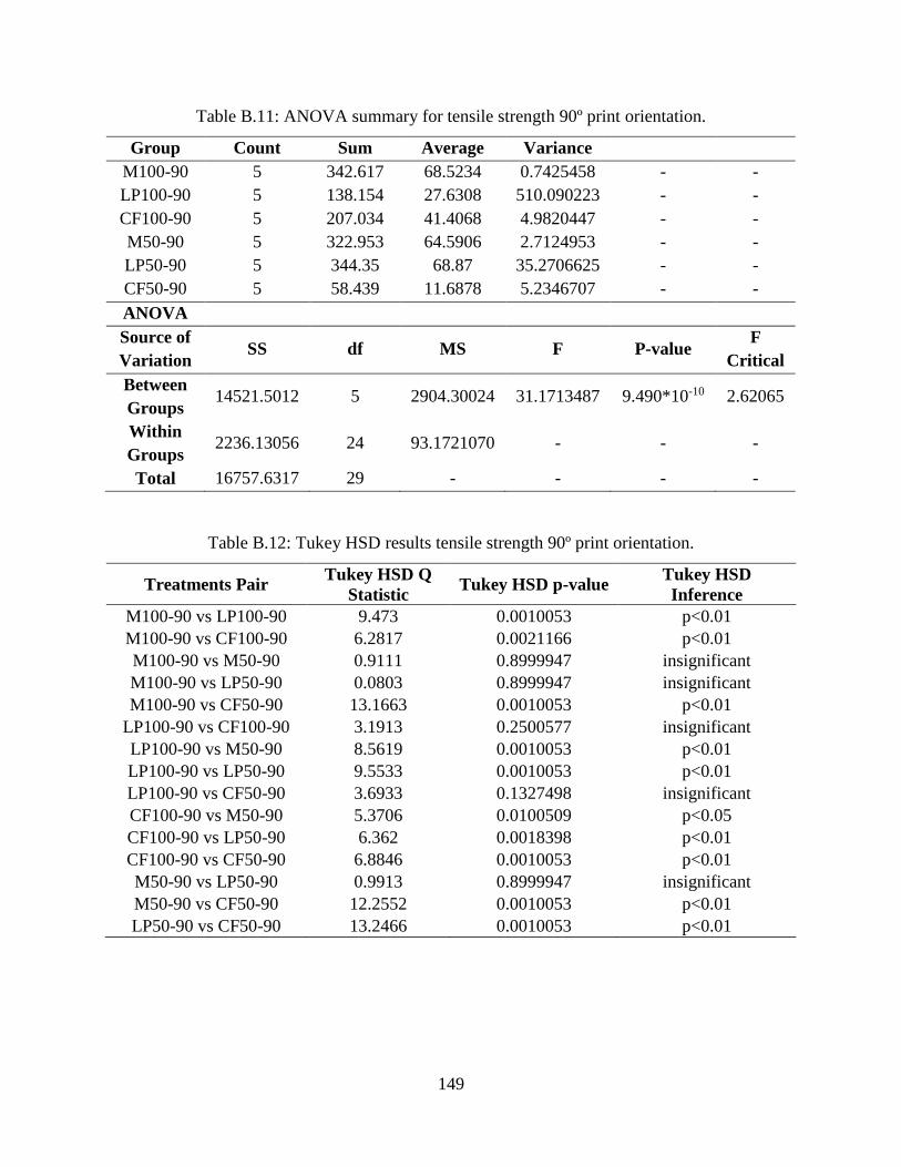
149

Table B.11: ANOVA summary for tensile strength 90º print orientation.


M100-90 5 342.617 68.5234 0.7425458 - -

LP100-90 5 138.154 27.6308 510.090223 - -

CF100-90 5 207.034 41.4068 4.9820447 - -

M50-90 5 322.953 64.5906 2.7124953 - -

LP50-90 5 344.35 68.87 35.2706625 - -

CF50-90 5 58.439 11.6878 5.2346707 - -

ANOVA

Source of


F

Critical

Between

Groups 14521.5012 5 2904.30024 31.1713487 9.490*10-10 2.62065

Within

Groups 2236.13056 24 93.1721070 - - -

Total 16757.6317 29 - - - -

Table B.12: Tukey HSD results tensile strength 90º print orientation.



Tukey HSD

Inference

M100-90 vs LP100-90 9.473 0.0010053 p<0.01

M100-90 vs CF100-90 6.2817 0.0021166 p<0.01



M100-90 vs CF50-90 13.1663 0.0010053 p<0.01


LP100-90 vs M50-90 8.5619 0.0010053 p<0.01

LP100-90 vs LP50-90 9.5533 0.0010053 p<0.01


CF100-90 vs M50-90 5.3706 0.0100509 p<0.05

CF100-90 vs LP50-90 6.362 0.0018398 p<0.01

CF100-90 vs CF50-90 6.8846 0.0010053 p<0.01


M50-90 vs CF50-90 12.2552 0.0010053 p<0.01

LP50-90 vs CF50-90 13.2466 0.0010053 p<0.01

150

Table B.13: ANOVA summary for tensile strength printed at 100 μm layer height.


M100-0 5 294.888 58.9776 25.7157088 - -

LP100-0 5 184.331 36.8662 63.8093842 - -

CF100-0 5 262.163 52.4326 13.3336853 - -

M100-90 5 342.617 68.5234 0.7425458 - -

LP100-90 5 138.154 27.6308 510.090223 - -

CF100-90 5 207.034 41.4068 4.9820447 - -

ANOVA

Source of


F

Critical

Between

Groups 5714.61108 5 1142.92221 11.0842508 1.287*10-5 2.62065

Within

Groups 2474.69436 24 103.112265 - - -

Total 8189.30544 29 - - - -

Table B.14: Tukey HSD results for tensile strength printed at 100 μm layer height.



Tukey HSD

Inference

M100-0 vs LP100-0 4.8691 0.0229462 p<0.05



M100-0 vs LP100-90 6.9028 0.0010053 p<0.01



LP100-0 vs M100-90 6.9711 0.0010053 p<0.01




CF100-0 vs LP100-90 5.4615 0.0086307 p<0.01


M100-90 vs LP100-90 9.0048 0.0010053 p<0.01

M100-90 vs CF100-90 5.9712 0.0036196 p<0.01


151

Table B.15: ANOVA summary for tensile strength printed at 50 μm layer height.


M50-0 5 217.372 43.4744 59.4877828 - -

LP50-0 5 251.5 50.3 62.082573 - -

CF50-0 5 252.942 50.5884 42.9189113 - -

M50-90 5 322.953 64.5906 2.7124953 - -

LP50-90 5 344.35 68.87 35.2706625 - -

CF50-90 5 58.439 11.6878 5.2346707 - -

ANOVA

Source of


F

Critical

Between

Groups 10307.3551 5 2061.47102 59.5493674 9.669*10-13 2.62065

Within

Groups 830.828382 24 34.6178492 - - -

Total 11138.1835 29 - - - -

Table B.16: Tukey HSD results for tensile strength printed at 50 μm layer height.



Tukey HSD

Inference



M50-0 vs M50-90 8.0251 0.0010053 p<0.01

M50-0 vs LP50-90 9.6515 0.0010053 p<0.01

M50-0 vs CF50-90 12.0803 0.0010053 p<0.01


LP50-0 vs M50-90 5.4311 0.0090823 p<0.01

LP50-0 vs LP50-90 7.0574 0.0010053 p<0.01

LP50-0 vs CF50-90 14.6744 0.0010053 p<0.01

CF50-0 vs M50-90 5.3215 0.0109131 p<0.05

CF50-0 vs LP50-90 6.9478 0.0010053 p<0.01

CF50-0 vs CF50-90 14.784 0.0010053 p<0.01


M50-0 vs LP50-0 20.1054 0.0010053 p<0.01

M50-0 vs CF50-0 21.7318 0.0010053 p<0.01

152

Table B.17: ANOVA summary for flexural modulus 0º print orientation.


M100-0 5 12.584 2.5168 0.0049087 - -

LP100-0 5 11.71 2.342 0.023488 - -

CF100-0 5 12.958 2.5916 0.0039833 - -

M50-0 5 12.737 2.5474 0.0001933 - -

LP50-0 5 11.129 2.2258 0.0439837 - -

CF50-0 5 13.229 2.6458 0.0121702 - -

ANOVA

Source of


F

Critical

Between

Groups

0.64742056 5 0.12948411 8.75610500 7.7833*10-5 2.62065

Within

Groups

0.3549088 24 0.01478786 - - -

Total 1.00232936 29 - - - -

Table B.18: Tukey HSD results flexural modulus 0º print orientation.



Tukey HSD

Inference




M100-0 vs LP50-0 5.3509 0.010389 p<0.05


LP100-0 vs CF100-0 4.5896 0.0357898 p<0.05



LP100-0 vs CF50-0 5.5862 0.0069875 p<0.01


CF100-0 vs LP50-0 6.7263 0.0010053 p<0.01


M50-0 vs LP50-0 5.9136 0.0039968 p<0.01


LP50-0 vs CF50-0 7.7229 0.0010053 p<0.01

153

Table B.19: ANOVA summary for flexural modulus 90º print orientation.


M100-90 5 12.105 2.421 0.0027865 - -

LP100-90 5 12.384 2.4768 0.0094907 - -

CF100-90 5 11.549 2.3098 0.0059202 - -

M50-90 5 13.146 2.6292 0.0032957 - -

LP50-90 5 12.505 2.501 0.0407685 - -

CF50-90 5 12.909 2.5818 0.0243977 - -

ANOVA

Source of


F

Critical

Between

Groups 0.326314 5 0.0652628 4.51857792 0.00481529 2.62065

Within

Groups 0.3466372 24 0.01444321 - - -

Total 0.6729512 29 - - - -

Table B.20: Tukey HSD results flexural modulus 90º print orientation.



Tukey HSD

Inference










CF100-90 vs M50-90 5.9428 0.0037998 p<0.01


CF100-90 vs CF50-90 5.0608 0.0168014 p<0.05




154

Table B.21: ANOVA summary for flexural modulus printed at 100 μm layer height.


M100-0 5 12.584 2.5168 0.0049087 - -

LP100-0 5 11.71 2.342 0.023488 - -

CF100-0 5 12.958 2.5916 0.0039833 - -

M100-90 5 12.105 2.421 0.0027865 - -

LP100-90 5 12.74 2.548 0.0537415 - -

CF100-90 5 11.549 2.3098 0.0059202 - -

ANOVA

Source of


F

Critical

Between

Groups 0.33067866 5 0.06613573 4.18456113 0.00708992 2.62065

Within

Groups 0.3793128 24 0.0158047 - - -

Total 0.70999146 29 - - - -

Table B.22: Tukey HSD results for flexural modulus printed at 100 μm layer height.



Tukey HSD

Inference






LP100-0 vs CF100-0 4.4395 0.0451671 p<0.05






CF100-0 vs CF100-90 5.0123 0.0181893 p<0.05




155

Table B.23: ANOVA summary for flexural modulus printed at 50 μm layer height.


M50-0 5 12.737 2.5474 0.0001933 - -

LP50-0 5 11.129 2.2258 0.0439837 - -

CF50-0 5 13.229 2.6458 0.0121702 - -

M50-90 5 13.146 2.6292 0.0032957 - -

LP50-90 5 12.505 2.501 0.0407685 - -

CF50-90 5 12.909 2.5818 0.0243977 - -

ANOVA

Source of


F

Critical

Between

Groups 0.59607376 5 0.11921475 5.73106063 0.00128690 2.62065

Within

Groups 0.4992364 24 0.02080151 - - -

Total 1.09531016 29 - - - -

Table B.24: Tukey HSD results for flexural modulus printed at 50 μm layer height.



Tukey HSD

Inference

M50-0 vs LP50-0 4.986 0.0189857 p<0.05





LP50-0 vs CF50-0 6.5116 0.0014191 p<0.01

LP50-0 vs M50-90 6.2542 0.0022196 p<0.01


LP50-0 vs CF50-90 5.5193 0.0078275 p<0.01







156

Table B.25: ANOVA summary for flexural strength 0º print orientation.


M100-0 5 430.15 86.03 88.7898 - -

LP100-0 5 139.67 27.934 29.15978 - -

CF100-0 5 424.87 84.974 18.13463 - -

M50-0 5 410.95 82.19 124.59595 - -

LP50-0 5 119.32 23.864 13.88708 - -

CF50-0 5 216.82 43.364 30.53483 - -

ANOVA

Source of


F

Critical

Between

Groups 21909.2795 5 4381.85590 86.1716061 1.566*10-14 2.62065

Within

Groups 1220.40828 24 50.850345 - - -

Total 23129.6877 29 - - - -

Table B.26: Tukey HSD results flexural strength 0º print orientation.



Tukey HSD

Inference

M100-0 vs LP100-0 18.2173 0.0010053 p<0.01



M100-0 vs LP50-0 19.4936 0.0010053 p<0.01

M100-0 vs CF50-0 13.3789 0.0010053 p<0.01

LP100-0 vs CF100-0 17.8862 0.0010053 p<0.01

LP100-0 vs M50-0 17.0132 0.0010053 p<0.01


LP100-0 vs CF50-0 4.8384 0.0241039 p<0.05


CF100-0 vs LP50-0 19.1624 0.0010053 p<0.01

CF100-0 vs CF50-0 13.0478 0.0010053 p<0.01

M50-0 vs LP50-0 18.2894 0.0010053 p<0.01

M50-0 vs CF50-0 12.1748 0.0010053 p<0.01

LP50-0 vs CF50-0 6.1147 0.002827 p<0.01

157

Table B.27: ANOVA summary for flexural strength 90º print orientation.


M100-90 5 480.77 96.154 3.04043 - -

LP100-90 5 73.17 14.634 9.05208 - -

CF100-90 5 330.25 66.05 110.18255 - -

M50-90 5 504.12 100.824 11.60793 - -

LP50-90 5 65.78 13.156 0.39383 - -

CF50-90 5 97.1 19.42 6.4429 - -

ANOVA

Source of


F

Critical

Between

Groups 42483.8722 5 8496.77444 362.285020 8.897*10-22 2.62065

Within

Groups 562.87888 24 23.4532866 - - -

Total 43046.7511 29 - - - -

Table B.28: Tukey HSD results flexural strength 90º print orientation.



Tukey HSD

Inference

M100-90 vs LP100-90 37.6398 0.0010053 p<0.01

M100-90 vs CF100-90 13.8998 0.0010053 p<0.01


M100-90 vs LP50-90 38.3222 0.0010053 p<0.01

M100-90 vs CF50-90 35.43 0.0010053 p<0.01

LP100-90 vs CF100-90 23.74 0.0010053 p<0.01

LP100-90 vs M50-90 39.7961 0.0010053 p<0.01



CF100-90 vs M50-90 16.056 0.0010053 p<0.01

CF100-90 vs LP50-90 24.4225 0.0010053 p<0.01

CF100-90 vs CF50-90 21.5302 0.0010053 p<0.01

M50-90 vs LP50-90 40.4785 0.0010053 p<0.01

M50-90 vs CF50-90 37.5862 0.0010053 p<0.01


158

Table B.29: ANOVA summary for flexural strength printed at 100 μm layer height.


M100-0 5 430.15 86.03 88.7898 - -

LP100-0 5 139.67 27.934 29.15978 - -

CF100-0 5 424.87 84.974 18.13463 - -

M100-90 5 480.77 96.154 3.04043 - -

LP100-90 5 73.17 14.634 9.05208 - -

CF100-90 5 330.25 66.05 110.18255 - -

ANOVA

Source of


F

Critical

Between

Groups 28448.9887 5 5689.79774 132.136874 1.187*10-16 2.62065

Within

Groups 1033.43708 24 43.0598783 - - -

Total 29482.4257 29 - - - -

Table B.30: Tukey HSD results for flexural strength printed at 100 μm layer height.



Tukey HSD

Inference

M100-0 vs LP100-0 19.7968 0.0010053 p<0.01



M100-0 vs LP100-90 24.3289 0.0010053 p<0.01

M100-0 vs CF100-90 6.8084 0.0010053 p<0.01

LP100-0 vs CF100-0 19.437 0.0010053 p<0.01

LP100-0 vs M100-90 23.2466 0.0010053 p<0.01

LP100-0 vs LP100-90 4.5321 0.0391507 p<0.05

LP100-0 vs CF100-90 12.9884 0.0010053 p<0.01


CF100-0 vs LP100-90 23.9691 0.0010053 p<0.01

CF100-0 vs CF100-90 6.4485 0.0015818 p<0.01

M100-90 vs LP100-90 27.7788 0.0010053 p<0.01

M100-90 vs CF100-90 10.2582 0.0010053 p<0.01

LP100-90 vs CF100-90 17.5205 0.0010053 p<0.01

159

Table B.31: ANOVA summary for flexural strength printed at 50 μm layer height.


M50-0 5 410.95 82.19 124.595 - -

LP50-0 5 119.32 23.86 13.887 - -

CF50-0 5 216.82 43.36 30.535 - -

M50-90 5 504.12 100.82 11.607 - -

LP50-90 5 65.78 13.16 0.394 - -

CF50-90 5 97.1 19.42 6.442 - -

ANOVA

Source of


F

Critical

Between

Groups 32949.0764 5 6589.81528 210.916249 5.179*10-19 2.62065

Within

Groups 749.85008 24 31.2437533 - - -

Total 33698.9265 29 - - - -

Table B.32: Tukey HSD results for flexural strength printed at 50 μm layer height.



Tukey HSD

Inference

M50-0 vs LP50-0 23.3327 0.0010053 p<0.01

M50-0 vs CF50-0 15.532 0.0010053 p<0.01

M50-0 vs M50-90 7.4543 0.0010053 p<0.01

M50-0 vs LP50-90 27.6164 0.0010053 p<0.01

M50-0 vs CF50-90 25.1105 0.0010053 p<0.01

LP50-0 vs CF50-0 7.8008 0.0010053 p<0.01

LP50-0 vs M50-90 30.7871 0.0010053 p<0.01



CF50-0 vs M50-90 22.9863 0.0010053 p<0.01

CF50-0 vs LP50-90 12.0844 0.0010053 p<0.01

CF50-0 vs CF50-90 9.5786 0.0010053 p<0.01

M50-90 vs LP50-90 35.0707 0.0010053 p<0.01

M50-0 vs LP50-0 32.5649 0.0010053 p<0.01


160

Table B.33: ANOVA summary for fracture toughness 0º print orientation.


M100-0 3 1.88 0.627 0.0158 - -

LP100-0 3 1.74 0.579 0.0333 - -

CF100-0 3 2.18 0.726 0.0215 - -

M50-0 3 1.96 0.654 0.0262 - -

LP50-0 3 1.67 0.565 0.00695 - -

CF50-0 3 1.72 0.573 0.00199 - -

ANOVA

Source of


F

Critical

Between

Groups 0.0579 5 0.0116 0.6567 0.6627 3.1059

Within

Groups 0.2116 12 0.0176 - - -

Total 0.2696 17 - - - -

Table B.34: Tukey HSD results fracture toughness 0º print orientation.



Tukey HSD

Inference
















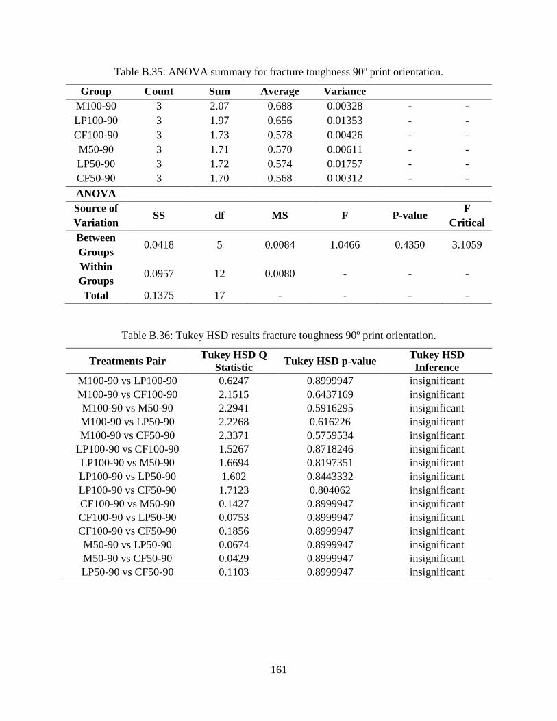
161

Table B.35: ANOVA summary for fracture toughness 90º print orientation.


M100-90 3 2.07 0.688 0.00328 - -

LP100-90 3 1.97 0.656 0.01353 - -

CF100-90 3 1.73 0.578 0.00426 - -

M50-90 3 1.71 0.570 0.00611 - -

LP50-90 3 1.72 0.574 0.01757 - -

CF50-90 3 1.70 0.568 0.00312 - -

ANOVA

Source of


F

Critical

Between

Groups 0.0418 5 0.0084 1.0466 0.4350 3.1059

Within

Groups 0.0957 12 0.0080 - - -

Total 0.1375 17 - - - -

Table B.36: Tukey HSD results fracture toughness 90º print orientation.



Tukey HSD

Inference
















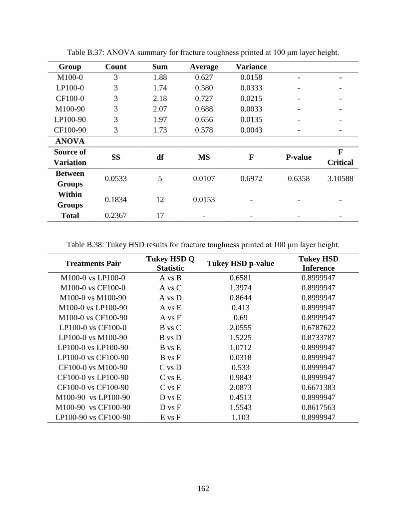
162

Table B.37: ANOVA summary for fracture toughness printed at 100 μm layer height.


M100-0 3 1.88 0.627 0.0158 - -

LP100-0 3 1.74 0.580 0.0333 - -

CF100-0 3 2.18 0.727 0.0215 - -

M100-90 3 2.07 0.688 0.0033 - -

LP100-90 3 1.97 0.656 0.0135 - -

CF100-90 3 1.73 0.578 0.0043 - -

ANOVA

Source of


F

Critical

Between

Groups 0.0533 5 0.0107 0.6972 0.6358 3.10588

Within

Groups 0.1834 12 0.0153 - - -

Total 0.2367 17 - - - -

Table B.38: Tukey HSD results for fracture toughness printed at 100 μm layer height.



Tukey HSD

Inference

M100-0 vs LP100-0 A vs B 0.6581 0.8999947

M100-0 vs CF100-0 A vs C 1.3974 0.8999947

M100-0 vs M100-90 A vs D 0.8644 0.8999947

M100-0 vs LP100-90 A vs E 0.413 0.8999947

M100-0 vs CF100-90 A vs F 0.69 0.8999947

LP100-0 vs CF100-0 B vs C 2.0555 0.6787622

LP100-0 vs M100-90 B vs D 1.5225 0.8733787

LP100-0 vs LP100-90 B vs E 1.0712 0.8999947

LP100-0 vs CF100-90 B vs F 0.0318 0.8999947

CF100-0 vs M100-90 C vs D 0.533 0.8999947

CF100-0 vs LP100-90 C vs E 0.9843 0.8999947

CF100-0 vs CF100-90 C vs F 2.0873 0.6671383

M100-90 vs LP100-90 D vs E 0.4513 0.8999947

M100-90 vs CF100-90 D vs F 1.5543 0.8617563

LP100-90 vs CF100-90 E vs F 1.103 0.8999947

163

Table B.39: ANOVA summary for fracture toughness printed at 50 μm layer height.


M50-0 3 1.96 0.654 0.0262 - -

LP50-0 3 1.70 0.565 0.0070 - -

CF50-0 3 1.72 0.573 0.0020 - -

M50-90 3 1.71 0.570 0.0061 - -

LP50-90 3 1.72 0.574 0.0176 - -

CF50-90 3 1.70 0.568 0.0031 - -

ANOVA

Source of


F

Critical

Between

Groups 0.0176 5 0.0035 0.3416 0.8780 3.10588

Within

Groups 0.1240 12 0.0103 - - -

Total 0.1416 17 - - - -

Table B.40: Tukey HSD results for fracture toughness printed at 50 μm layer height.



Tukey HSD

Inference
















ADDITIVE MANUFACTURING OF SHORT-FIBER COMPOSITES VIA ...

Documents

Transcript of ADDITIVE MANUFACTURING OF SHORT-FIBER COMPOSITES VIA ...