additionals Macros for pstricks

pstricksadd

additionals Macros for pstricksv.2.82

Dominique Rodriguez and Herbert Voß

November 27, 2006

Abstract

This version of pstricksadd needs pstricks.tex version >1.04 from June 2004,otherwise the additional macros may not work as espected. The ellipsis materialand the option asolid (renamed to eofill) are now part of the new pstricks.tex

package, available at CTAN or at http://perce.de/LaTeX/. pstricksadd will forever be an experimental and dynamical package, try it at your own risk.

• It is important to load pstricksadd as last PSTricks related package, otherwisea lot of the macros won’t work in the expected way.

• pstricksadd uses the extended version of the keyval package. So be sure, thatyou have installed pstxkey which is part of the xkeyval-package and that allpackages, that uses the old keyval interface are loaded before the xkeyval.[1]

• the option tickstyle from pstplot is no more supported, use ticksize in-stead.

• the option xyLabel is no more supported, use the option labelFontSize in-stead.

1

http://perce.de/LaTeX/

Contents

I pstricks 7

1 Numeric functions . . . . . . . . . . . . . . . . . . . . . . . . . . . . . . . . . 7

1.1 \pst@divide . . . . . . . . . . . . . . . . . . . . . . . . . . . . . . . . . 7

1.2 \pst@mod . . . . . . . . . . . . . . . . . . . . . . . . . . . . . . . . . . . 7

1.3 \pst@max . . . . . . . . . . . . . . . . . . . . . . . . . . . . . . . . . . . 8

1.4 \pst@maxdim . . . . . . . . . . . . . . . . . . . . . . . . . . . . . . . . . 8

1.5 \pst@abs . . . . . . . . . . . . . . . . . . . . . . . . . . . . . . . . . . . 8

1.6 \pst@absdim . . . . . . . . . . . . . . . . . . . . . . . . . . . . . . . . . 8

1.7 Reading angle values . . . . . . . . . . . . . . . . . . . . . . . . . . . 9

2 Dashed Lines . . . . . . . . . . . . . . . . . . . . . . . . . . . . . . . . . . . . 9

3 \rmultiput: a multiple \rput . . . . . . . . . . . . . . . . . . . . . . . . . . 10

4 \psrotate: Rotating objects . . . . . . . . . . . . . . . . . . . . . . . . . . . . 10

5 \psbrace . . . . . . . . . . . . . . . . . . . . . . . . . . . . . . . . . . . . . . . 11

5.1 Syntax . . . . . . . . . . . . . . . . . . . . . . . . . . . . . . . . . . . . 11

5.2 Options . . . . . . . . . . . . . . . . . . . . . . . . . . . . . . . . . . . 11

6 Random dots . . . . . . . . . . . . . . . . . . . . . . . . . . . . . . . . . . . . 16

7 Arrows . . . . . . . . . . . . . . . . . . . . . . . . . . . . . . . . . . . . . . . . 18

7.1 Definition . . . . . . . . . . . . . . . . . . . . . . . . . . . . . . . . . . 18

7.2 Multiple arrows . . . . . . . . . . . . . . . . . . . . . . . . . . . . . . . 18

7.3 hookarrow . . . . . . . . . . . . . . . . . . . . . . . . . . . . . . . . . . 20

7.4 hookrightarrow and hookleftarrow . . . . . . . . . . . . . . . . . . 20

7.5 ArrowInside Option . . . . . . . . . . . . . . . . . . . . . . . . . . . . 21

7.6 ArrowFill Option . . . . . . . . . . . . . . . . . . . . . . . . . . . . . 22

7.7 Examples . . . . . . . . . . . . . . . . . . . . . . . . . . . . . . . . . . 23

7.7.1 \psline . . . . . . . . . . . . . . . . . . . . . . . . . . . . . . 23

7.7.2 \pspolygon . . . . . . . . . . . . . . . . . . . . . . . . . . . . 25

7.7.3 \psbezier . . . . . . . . . . . . . . . . . . . . . . . . . . . . 26

7.7.4 \pcline . . . . . . . . . . . . . . . . . . . . . . . . . . . . . . 28

7.7.5 \pccurve . . . . . . . . . . . . . . . . . . . . . . . . . . . . . 29

8 \psFormatInt . . . . . . . . . . . . . . . . . . . . . . . . . . . . . . . . . . . . 30

2

9 Color . . . . . . . . . . . . . . . . . . . . . . . . . . . . . . . . . . . . . . . . . 30

9.1 Transparent colors . . . . . . . . . . . . . . . . . . . . . . . . . . . . . 30

9.2 „Manipulating Transparent colors” . . . . . . . . . . . . . . . . . . . 31

9.3 Calculated colors . . . . . . . . . . . . . . . . . . . . . . . . . . . . . . 32

9.4 Gouraud shading . . . . . . . . . . . . . . . . . . . . . . . . . . . . . . 35

II pstnode 38

10 \ncdiag and \pcdiag . . . . . . . . . . . . . . . . . . . . . . . . . . . . . . . 38

11 \ncdiagg and \pcdiagg . . . . . . . . . . . . . . . . . . . . . . . . . . . . . . 39

12 \ncbarr . . . . . . . . . . . . . . . . . . . . . . . . . . . . . . . . . . . . . . . 41

13 \psRelNode . . . . . . . . . . . . . . . . . . . . . . . . . . . . . . . . . . . . . 42

14 \psRelLine . . . . . . . . . . . . . . . . . . . . . . . . . . . . . . . . . . . . . 42

15 \psParallelLine . . . . . . . . . . . . . . . . . . . . . . . . . . . . . . . . . . 46

16 \psIntersectionPoint . . . . . . . . . . . . . . . . . . . . . . . . . . . . . . 47

17 \psLNode and \psLCNode . . . . . . . . . . . . . . . . . . . . . . . . . . . . . 48

18 \nlput and \psLDNode . . . . . . . . . . . . . . . . . . . . . . . . . . . . . . . 49

III pstplot 50

19 New options . . . . . . . . . . . . . . . . . . . . . . . . . . . . . . . . . . . . 50

19.1 Changing the label font size with labelFontSize . . . . . . . . . . . 52

19.2 algebraic . . . . . . . . . . . . . . . . . . . . . . . . . . . . . . . . . . 53

19.2.1 Using the Sum function . . . . . . . . . . . . . . . . . . . . . 55

19.2.2 Using the IfTE function . . . . . . . . . . . . . . . . . . . . 56

19.3 comma . . . . . . . . . . . . . . . . . . . . . . . . . . . . . . . . . . . . . 58

19.4 xyAxes, xAxis and yAxis . . . . . . . . . . . . . . . . . . . . . . . . . 58

19.5 xyDecimals, xDecimals and yDecimals . . . . . . . . . . . . . . . . . 59

19.6 ticks . . . . . . . . . . . . . . . . . . . . . . . . . . . . . . . . . . . . . 60

19.7 labels . . . . . . . . . . . . . . . . . . . . . . . . . . . . . . . . . . . . 61

19.8 ticksize, xticksize, yticksize . . . . . . . . . . . . . . . . . . . . . 62

19.9 subticks . . . . . . . . . . . . . . . . . . . . . . . . . . . . . . . . . . . 63

19.10 subticksize, xsubticksize, ysubticksize . . . . . . . . . . . . . . 64

19.11 tickcolor, subtickcolor . . . . . . . . . . . . . . . . . . . . . . . . . 65

3

19.12 ticklinestyle and subticklinestyle . . . . . . . . . . . . . . . . . 65

19.13 loglines . . . . . . . . . . . . . . . . . . . . . . . . . . . . . . . . . . . 66

19.14 xylogBase, xlogBase and ylogBase . . . . . . . . . . . . . . . . . . . 68

19.14.1 xylogBase . . . . . . . . . . . . . . . . . . . . . . . . . . . . 68

19.14.2 ylogBase . . . . . . . . . . . . . . . . . . . . . . . . . . . . . 69

19.14.3 xlogBase . . . . . . . . . . . . . . . . . . . . . . . . . . . . . 71

19.14.4 No logstyle (xylogBase={}) . . . . . . . . . . . . . . . . . . 72

19.15 subticks, tickwidth and subtickwidth . . . . . . . . . . . . . . . . 73

19.16 xlabelFactor and ylabelFactor . . . . . . . . . . . . . . . . . . . . 78

19.17 Plot style bar and option barwidth . . . . . . . . . . . . . . . . . . . 79

19.18 trigLabels and trigLabelBase – axis with trigonmetrical units . . 80

19.19 New options for \readdata . . . . . . . . . . . . . . . . . . . . . . . . 84

19.20 New options for \listplot . . . . . . . . . . . . . . . . . . . . . . . . 85

19.20.1 Example for nStep/xStep . . . . . . . . . . . . . . . . . . . 86

19.20.2 Example for nStart/xStart . . . . . . . . . . . . . . . . . . 86

19.20.3 Example for nEnd/xEnd . . . . . . . . . . . . . . . . . . . . . 87

19.20.4 Example for all new options . . . . . . . . . . . . . . . . . . 87

19.20.5 Example for xStart . . . . . . . . . . . . . . . . . . . . . . . 88

19.20.6 Example for yStart/yEnd . . . . . . . . . . . . . . . . . . . 89

19.20.7 Example for plotNo/plotNoMax . . . . . . . . . . . . . . . . 89

19.20.8 Example for changeOrder . . . . . . . . . . . . . . . . . . . 91

20 Polar plots . . . . . . . . . . . . . . . . . . . . . . . . . . . . . . . . . . . . . . 91

21 \pstScalePoints . . . . . . . . . . . . . . . . . . . . . . . . . . . . . . . . . . 93

IV New commands and environments 94

22 psgraph environment . . . . . . . . . . . . . . . . . . . . . . . . . . . . . . . 94

22.1 The new options . . . . . . . . . . . . . . . . . . . . . . . . . . . . . . 100

22.2 Problems . . . . . . . . . . . . . . . . . . . . . . . . . . . . . . . . . . . 101

23 \psStep . . . . . . . . . . . . . . . . . . . . . . . . . . . . . . . . . . . . . . . 102

24 \psplotTangent . . . . . . . . . . . . . . . . . . . . . . . . . . . . . . . . . . 104

24.1 A polarplot example . . . . . . . . . . . . . . . . . . . . . . . . . . . 106

24.2 A \parametricplot example . . . . . . . . . . . . . . . . . . . . . . . 107

4

25 Successive derivatives of a function . . . . . . . . . . . . . . . . . . . . . . . 108

26 Variable step for plotting a curve . . . . . . . . . . . . . . . . . . . . . . . . . 110

26.1 Theory . . . . . . . . . . . . . . . . . . . . . . . . . . . . . . . . . . . . 110

26.2 The cosine . . . . . . . . . . . . . . . . . . . . . . . . . . . . . . . . . . 110

26.3 The neperian Logarithm . . . . . . . . . . . . . . . . . . . . . . . . . . 111

26.4 Sinus of the inverse of x . . . . . . . . . . . . . . . . . . . . . . . . . . 112

26.5 A really complex function . . . . . . . . . . . . . . . . . . . . . . . . . 112

26.6 A hyperbola . . . . . . . . . . . . . . . . . . . . . . . . . . . . . . . . . 113

26.7 Successive derivatives of a polynom . . . . . . . . . . . . . . . . . . . 114

26.8 The variable step algorithm together with the IfTE primitive . . . . 115

26.9 Using \parametricplot . . . . . . . . . . . . . . . . . . . . . . . . . . 115

27 New math functions and their derivative . . . . . . . . . . . . . . . . . . . . 117

27.1 The inverse sin and its derivative . . . . . . . . . . . . . . . . . . . . 117

27.2 The inverse cosine and its derivative . . . . . . . . . . . . . . . . . . . 118

27.3 The inverse tangente and its derivative . . . . . . . . . . . . . . . . . 119

27.4 Hyperbolique functions . . . . . . . . . . . . . . . . . . . . . . . . . . 120

28 \psplotDiffEqn – solving diffential equations . . . . . . . . . . . . . . . . . 124

28.1 Variable step for differential equations . . . . . . . . . . . . . . . . . 125

28.2 Equation of second order . . . . . . . . . . . . . . . . . . . . . . . . . 128

28.2.1 Simple equation of first order y′ = y . . . . . . . . . . . . . 130

28.2.2 y′ =2 − ty

4 − t2. . . . . . . . . . . . . . . . . . . . . . . . . . . . 131

28.2.3 y′ = −2xy . . . . . . . . . . . . . . . . . . . . . . . . . . . . . 133

28.2.4 Spirale of Cornu . . . . . . . . . . . . . . . . . . . . . . . . . 133

28.2.5 Lotka-Volterra . . . . . . . . . . . . . . . . . . . . . . . . . . 134

28.2.6 y′′ = y . . . . . . . . . . . . . . . . . . . . . . . . . . . . . . . 136

28.2.7 y′′ = −y . . . . . . . . . . . . . . . . . . . . . . . . . . . . . . 137

28.2.8 The mechanical pendulum: y′′ = −g

lsin(y) . . . . . . . . . . 138

28.2.9 y′′ = −y′

4− 2y . . . . . . . . . . . . . . . . . . . . . . . . . . . 139

29 \psMatrixPlot . . . . . . . . . . . . . . . . . . . . . . . . . . . . . . . . . . . 140

30 \psforeach . . . . . . . . . . . . . . . . . . . . . . . . . . . . . . . . . . . . . 142

31 \resetOptions . . . . . . . . . . . . . . . . . . . . . . . . . . . . . . . . . . . 143

A PostScript . . . . . . . . . . . . . . . . . . . . . . . . . . . . . . . . . . . . . . 143

5

B Credits . . . . . . . . . . . . . . . . . . . . . . . . . . . . . . . . . . . . . . . . 143

C Change log . . . . . . . . . . . . . . . . . . . . . . . . . . . . . . . . . . . . . 145

6

Part I

pstricks

1 Numeric functions

All macronames contain a @ in their name, because they are only for internal use, but itis no problem to use it as the other macros. One can define another name without a @:

\makeatletter

\let\pstdivide\pst@divide

\makeatother

or put the macro inside of the \makeatletter – \makeatother sequence.

1.1 \pst@divide

pstricks itself has its own divide macro, called \pst@divide which can divide two lengthesand saves the quotient as a floating point number:

\pst@divide{<dividend>}{<divisor>}{<result as a macro>}

5.66666-0.17647

1 \makeatletter

2 \pst@divide{34pt}{6pt}\quotient \quotient\\

3 \pst@divide{6pt}{34pt}\quotient \quotient

4 \makeatother

this gives the output 5.66666. The result is not a length!

1.2 \pst@mod

pstricksadd defines an additional numeric function for the modulus:

\pst@mod{<integer>}{<integer>}{<result as a macro>}

41

1 \makeatletter

2 \pst@mod{34}{6}\modulo \modulo\\

3 \pst@mod{25}{6}\modulo \modulo

4 \makeatother

this gives the output 4. Using this internal numeric functions in documents requires asetting inside the makeatletter and makeatother environment. It makes some sense todefine a new macroname in the preamble to use it throughou, e.g. \let\modulo\pst@mod.

7

1.3 \pst@max

\pst@max{<integer>}{<integer>}{<result as count register>}

-611

1 \newcount\maxNo

2 \makeatletter

3 \pst@max{34}{6}\maxNo \the\maxNo\\

4 \pst@max{0}{11}\maxNo \the\maxNo

5 \makeatother

1.4 \pst@maxdim

\pst@maxdim{<dimension>}{<dimension>}{<result as dimension register>}

1234.0pt967.39369pt

1 \newdimen\maxDim

2 \makeatletter

3 \pst@maxdim{34cm}{1234pt}\maxDim \the\maxDim\\

4 \pst@maxdim{34cm}{123pt}\maxDim \the\maxDim

5 \makeatother

1.5 \pst@abs

\pst@abs{<integer>}{<result as a count register>}

344

1 \newcount\absNo

2 \makeatletter

3 \pst@abs{34}\absNo \the\absNo\\

4 \pst@abs{4}\absNo \the\absNo

5 \makeatother

1.6 \pst@absdim

\pst@absdim{<dimension>}{<result as a dimension register>}

967.39369pt0.00006pt

1 \newdimen\absDim

2 \makeatletter

3 \pst@absdim{34cm}\absDim \the\absDim\\

4 \pst@absdim{4sp}\absDim \the\absDim

5 \makeatother

8

1.7 Reading angle values

By default PSTricks checks the input value of angles. With the optional argumentangleCheck this internal check can be disabled. Then PSTricks passes the input straightto PostScript and it is possible to do some calculating by using PostScript code.

1 \def\angleA{0 }% space after value

2 \def\angleB{45 }

3 \begin{pspicture}(4,3)

4 \psarc[angleCheck=false,linecolor=red,showpoints=true]%

5 (0,0){3}{ \angleA }{ \angleB 0.5 mul 30 add }

6 \end{pspicture}

Without disabling the angle check, the above code causes an error because of the secondargument, which is not a correct angle value.

2 Dashed Lines

Tobias Nähring implemented an enhanced feature for dashed lines. The number of ar-guments is no more limited.

dash=value1[unit] value2[unit] ...

1 \psset{linewidth=2.5pt,unit=0.6}

2 \begin{pspicture}(5,4)(5,4)

3 \psgrid[subgriddiv=0,griddots=10,gridlabels=0

pt]

4 \psset{linestyle=dashed}

5 \pscurve[dash=5mm 1mm 1mm 1mm,linewidth

=0.1](5,4)(4,3)(3,4)(2,3)

6 \psline[dash=5mm 1mm 1mm 1mm 1mm 1mm 1mm 1mm

1mm 1mm](5,0.9)(5,0.9)

7 \psccurve[linestyle=solid](0,0)(1,0)(1,1)

(0,1)

8 \psccurve[linestyle=dashed,dash=5mm 2mm 0.1

0.2,linetype=0](0,0)(2.5,0)(2.5,2.5)

(0,2.5)

9 \pscurve[dash=3mm 3mm 1mm 1mm,linecolor=red,

linewidth=2pt](5,4)(5,2)(4.5,3.5)(3,4)

(5,4)

10 \end{pspicture}

9

3 \rmultiput: a multiple \rput

PSTricks already knows a multirput, which puts a box n times with a difference of dxand dy relativ to each other. It is not possible to put it with a different distance from onepoint to the next one. This is possible with rmultiput:

\rmultiput[<options>]{<any material>}(x1,y1)(x2,y2) ... (xn,yn)

\rmultiput*[<options>]{<any material>}(x1,y1)(x2,y2) ... (xn,yn)

➺➺➺➺

➺➺➺ ➺➽➽➽

➽

➽➽ ➽

-4 -3 -2 -1 0 1 2 3 4-4

-3

-2

-1

0

1

2

3

4

1 \psset{unit=0.75}


3 \rmultiput[rot=45]{\red\psscalebox{3}{\ding

{250}}}%

4 (2,4)(2,3)(3,3)(2,1)(0,0)(1,2)(1.5,3)

(3,3)

5 \rmultiput[rot=90,ref=lC]{\blue\psscalebox{2}{\

ding{253}}}%

6 (2,2.5)(2,2.5)(3,2.5)(2,1)(1,2)(1.5,3)

(3,3)

7 \psgrid[subgriddiv=0,gridcolor=lightgray]

8 \end{pspicture}

4 \psrotate: Rotating objects

\rput also has an optional argument for rotating objects, but always depending to the\rput coordinates. With \psrotate the rotating center can be placed anywhere. Therotation is done with \pscustom, all optional arguments are only valid if they are part ofthe \pscustom macro.

\psrotate[options](x,y){rot angle}{<object>}

1

2

3

4

−1

−2

−3

1 2 3 4 5 6 7 8

�

1 \psset{unit=0.75}

2 \begin{pspicture}(0.5,3.5)(8.5,4.5)

3 \psaxes{>}(0,0)(0.5,3)(8.5,4.5)

4 \psdots[linecolor=red,dotscale=1.5](2,1)

5 \psarc[linecolor=red,linewidth=0.4pt,

showpoints=true]

6 {>}(2,1){3}{0}{60}

7 \pspolygon[linecolor=green,linewidth=1pt

](2,1)(5,1.1)(6,1)(2,2)

8 \psrotate[linecolor=blue,linewidth=1pt](2,1)

{60}{

9 \pspolygon(2,1)(5,1.1)(6,1)(2,2)}

10 \end{pspicture}

10

5 \psbrace

5.1 Syntax

\psbrace[<options>](<A>)(<B>){<text>}

0 1 2 3 40

1

2

3

4

Text I

Text

II 1 \begin{pspicture}(4,4)

2 \psgrid[subgriddiv=0,griddots=10]

3 \pnode(0,0){A}

4 \pnode(4,4){B}

5 \psbrace[linecolor=red,ref=lC](A)(B){Text I}

6 \psbrace[linecolor=blue,ref=lC](3,4)(0,1){Text II}

7 \end{pspicture}

The option \specialCoor is enabled, so that all types of coordinates are possible, (node-name), (x, y), (nodeA|nodeB), ...

5.2 Options

Additional to all other available options from pstricks or the other related packages,there are two new option, named braceWidth and bracePos. All important ones are shownin the following table.

name meaningbraceWidth default is 0.35bracePos relative position (default is 0.5)linearc absolute value for the arcs (default is 2mm)nodesepA x-separation (default is 0pt)nodesepB y-separation (default is 0pt)rot additional rotating for the text (default is 0)ref reference point for the text (default is c)

By default the text is written perpedicular to the brace line and can be changed with thepstricks option rot=.... The text parameter can take any object and may also be empty.The reference point can be any value of the combination of l (left) or r (right) and b

(bottom) or B (Baseline) or C (center) or t (top), where the default is c, the center of theobject.

11

Text Text Text

Tex

t Tex

t

1 \begin{pspicture}(8,2.5)

2 \psbrace(0,0)(0,2){\fbox{Text}}%

3 \psbrace[nodesepA=20pt](2,0)(2,2){\

fbox{Text}}

4 \psbrace[ref=lC](4,0)(4,2){\fbox{Text

}}

5 \psbrace[ref=lt,rot=90,nodesepB=15pt

](6,0)(6,2){\fbox{Text}}

6 \psbrace[ref=lt,rot=90,nodesepA=5pt,

nodesepB=15pt](8,2)(8,0){\fbox{Text

}}

7 \end{pspicture}

∞∫

1

1x2 dx = 1

∞∫

1

1x2 dx = 1

∞∫

1

1x2 dx = 1

∞ ∫ 1

1 x2dx=

1

∞∫1

1x2dx=

1

1 \def\someMath{$\int\limits_1^{\infty

}\frac{1}{x^2}\,dx=1$}


3 \psbrace(0,0)(0,2){\someMath}%

4 \psbrace[nodesepA=30pt](2,0)(2,2){\

someMath}

5 \psbrace[ref=lC](4,0)(4,2){\someMath}


](6,0)(6,2){\someMath}


](8,2)(8,0){\someMath}

8 \end{pspicture}

Tex

t

Text

some very, very long wonderful Text

1 \begin{pspicture}(\linewidth,5)

2 \psbrace(0,0.5)(\linewidth,0.5){\fbox

{Text}}%

3 \psbrace[bracePos=0.25,nodesepB=10pt

,rot=90](0,2)(\linewidth,2){\fbox{

Text}}

4 \psbrace[ref=lC,nodesepA=3.5cm,

nodesepB=15pt,rot=90](0,4)(\

linewidth,4){%

5 \fbox{some very, very long

wonderful Text}}

6 \end{pspicture}

12

0 1 2 3 4 5 6 7 8 9 100

1

2

3

4

5

6

7

8

9

10

11

One

Two Three

Four A

I

II

III

IV

1 \psset{unit=0.8}



4 \pnode(0,0){A}

5 \pnode(4,6){B}

6 \psbrace[ref=lC](A)(B){One}

7 \psbrace[rot=180,nodesepA=5pt,ref=rb](B)(A){Two

}

8 \psbrace[linecolor=blue,bracePos=0.25,braceWidth

=1,ref=lB](8,1)(1,7){Three}

9 \psbrace[braceWidth=1,rot=180,ref=rB](8,1)(1,7)

{Four}

10 \psbrace[linearc=0.5,linecolor=red,linewidth=3pt

,braceWidth=1.5,%

11 bracePos=0.25,ref=lC](8,1)(8,9){A}

12 \psbrace(4,9)(6,9){}

13 \psbrace(6,9)(6,7){}

14 \psbrace(6,7)(4,7){}

15 \psbrace(4,7)(4,9){}

16 \psset{linecolor=red}

17 \psbrace[ref=lb](7,10)(3,10){I}

18 \psbrace[ref=lb,bracePos=0.75](3,10)(3,6){II}

19 \psbrace[ref=lb](3,6)(7,6){III}

20 \psbrace[ref=lb](7,6)(7,10){IV}

21 \end{pspicture}

1. . .

10

. . .

0

ntim

es

ntim

es

1 \[

2 \begin{pmatrix}

3 \Rnode[vref=2ex]{A}{~1} \\

4 & \ddots \\

5 && \Rnode[href=2]{B}{1} \\

6 &&& \Rnode[vref=2ex]{C}{0} \\

7 &&&& \ddots \\

8 &&&&& \Rnode[href=2]{D}{0}~ \\

9 \end{pmatrix}

10 \]

11 \psbrace[linewidth=0.1pt,rot=90,nodesep=0.2](B)(A){\small n

times}

12 \psbrace[linewidth=0.1pt,rot=90,nodesep=0.2](D)(C){\small n

times}

It is also possible to put a vertical brace around a default paragraph. This works withsetting two invisible nodes at the beginning and the end of the paragraph. Inentation ispossible with a minipage.

13

Some nonsense text, which is nothing more than nonsense. Some nonsense text,which is nothing more than nonsense.

Some nonsense text, which is nothing more than nonsense. Some nonsense text,which is nothing more than nonsense. Some nonsense text, which is nothing morethan nonsense. Some nonsense text, which is nothing more than nonsense. Somenonsense text, which is nothing more than nonsense. Some nonsense text, whichis nothing more than nonsense. Some nonsense text, which is nothing more thannonsense. Some nonsense text, which is nothing more than nonsense.

Some nonsense text, which is nothing more than nonsense. Some nonsense text,which is nothing more than nonsense.

Some nonsense text, which is nothing more than nonsense. Some nonsense text,which is nothing more than nonsense. Some nonsense text, which is nothingmore than nonsense. Some nonsense text, which is nothing more than nonsense.Some nonsense text, which is nothing more than nonsense. Some nonsense text,which is nothing more than nonsense. Some nonsense text, which is nothingmore than nonsense. Some nonsense text, which is nothing more than nonsense.

1 \begin{framed}

2 Some nonsense text, which is nothing more than nonsense.


4

5 \noindent\rnode{A}{}

6

7 \vspace*{1ex}









16

17 \vspace*{2ex}

18 \noindent\rnode{B}{}\psbrace[linecolor=red](A)(B){}

19



22

23 \medskip

24 \hfill\begin{minipage}{0.95\linewidth}

25 \noindent\rnode{A}{}

14

26

27 \vspace*{1ex}









36

37 \vspace*{2ex}

38 \noindent\rnode{B}{}\psbrace[linecolor=red](A)(B){}

39 \end{minipage}

40 \end{framed}

15

6 Random dots

The syntax of the new macro \psRandom is:

\psRandom[<option>]{}

\psRandom[<option>]{<clip path>}

\psRandom[<option>](<xMax,yMax>){<clip path>}

\psRandom[<option>](<xMin,yMin>)(<xMax,yMax>){<clip path>}

If there is no area for the dots defined, then (0,0)(1,1) in the actual scale is used forplacing the dots. This area should be greater than the clipping path to be sure that thedots are placed over the full area. The clipping path can be everything. If no clippingpath is given, then the frame (0,0)(1,1) in user coordinates is used. The new optionsare:

name defaultrandomPoints 1000 number of random dotscolor false random color

�

�

�

�

�

�

�

�

�

�

�

�

�

�

�

�

�

�

�

�

�

�

�

�

�

�

�

�

�

�

�

�

�

�

�

�

�

�

�

�

�

�

�

�

�

�

�

��

�

�

�

�

�

�

�

�

�

�

�

�

�

�

�

�

�

�

�

�

�

�

�

�

�

�

�

�

�

�

�

�

�

�

�

�

�

�

�

�

��

�

�

�

�

�

�

�

�

�

�

�

�

�

�

�

�

�

�

�

�

�

�

�

�

�

�

�

�

�

�

�

�

�

�

�

�

�

�

��

�

�

�

�

�

�

�

�

�

�

�

�

�

�

�

�

�

�

�

�

�

�

�

�

�

�

�

�

�

�

�

�

�

�

�

�

�

�

�

�

�

��

�

�

�

�

�

�

�

�

�

�

�

�

�

�

�

�

�

�

�

�

�

�

�

�

�

�

�

�

�

�

�

�

�

�

�

�

�

�

�

�

�

�

�

�

�

�

�

�

�

�

�

�

�

�

�

�

�

�

�

�

�

�

�

�

�

�

�

�

�

�

�

�

�

�

�

�

�

�

��

�

�

�

�

�

�

�

�

�

�

�

�

�

�

�

�

�

�

�

�

�

�

�

�

�

�

�

�

�

�

�

�

�

�

�

�

�

�

�

�

�

�

�

�

�

�

�

�

�

�

�

�

�

�

�

�

�

� �

�

�

�

�

�

�

�

�

�

�

�

�

�

�

�

�

�

�

�

�

�

�

�

�

�

�

�

�

�

�

�

�

�

�

�

�

�

�

�

�

�

�

�

�

�

�

�

�

�

�

�

�

� �

�

�

�

�

�

�

�

�

�

�

�

�

�

��

�

�

�

�

�

�

�

�

�

�

�

�

�

�

��

�

�

�

�

�

�

�

�

�

�

�

�

�

�

�

�

�

�

�

�

�

�

�

�

�

�

�

�

�

�

�

�

�

�

�

�

�

��

�

�

�

�

�

�

�

�

�

�

�

�

�

�

�

�

�

�

�

�

�

�

�

�

�

�

�

�

�

�

�

�

�

�

�

�

�

�

�

�

�

�

�

�

�

�

�

�

�

�

�

�

�

�

�

�

�

�

�

�

�

�

�

�

�

�

�

�

�

�

�

�

�

�

�

�

�

�

�

�

�

�

�

�

�

�

�

�

�

�

�

�

�

�

��

�

�

�

�

�

�

�

�

�

�

�

�

�

�

�

�

�

�

�

�

�

�

�

�

�

�

�

�

�

�

�

�

�

�

�

�

�

�

�

�

�

�

�

�

�

�

�

�

�

�

�

�

�

�

�

�

��

�

�

�

�

�

�

�

�

�

�

�

�

�

�

�

�

�

�

�

�

�

�

�

�

�

�

�

�

�

�

�

�

�

�

�

�

�

�

�

�

�

�

�

�

�

�

�

�

�

�

�

�

�

�

�

�

�

�

�

�

�

�

�

�

�

�

�

�

�

�

�

�

�

�

�

�

�

�

�

�

�

� �

�

�

�

�

�

�

�

�

�

�

�

�

�

�

�

�

�

�

�

�

�

�

�

�

�

�

�

�

�

�

�

�

�

�

�

�

�

�

�

�

�

�

�

�

�

�

�

�

�

�

�

�

�

�

�

�

�

�

�

�

�

�

�

�

�

�

�

�

�

�

�

�

�

�

�

�

�

�

�

�

�

�

�

�

�

�

�

�

�

�

�

�

�

�

�

�

�

�

�

�

�

�

�

�

�

�

�

�

�

�

�

�

�

�

�

�

�

�

�

�

�

�

�

�

�

�

�

�

�

�

�

�

�

�

�

�

�

�

�

�

�

�

�

�

�

�

�

�

�

�

�

�

��

�

�

�

�

�

�

�

�

�

�

�

�

�

�

�

�

�

�

�

�

�

�

�

�

�

�

�

�

�

�

�

�

�

�

�

�

�

�

�

�

�

�

�

�

�

�

�

�

�

�

�

�

�

�

�

�

�

�

�

�

�

�

�

�

�

�

�

�

�

�

�

�

�

�

�

�

�

�

�

�

�

�

�

�

�

�

�

�

�

�

�

�

�

�

�

�

��

�

�

�

�

�

�

�

�

�

�

�

�

�

�

�

�

�

�

�

�

�

�

�

�

�

�

�

�

�

�

�

�

�

�

�

�

�

�

�

�

�

�

�

�

�

�

�

�

�

�

�

�

�

�

�

��

�

�

�

�

�

�

�

�

�

�

�

�

�

�

�

�

�

�

��

�

�

�

�

�

�

�

�

�

�

�

�

�

�

�

�

�

�

�

�

�

�

�

�

�

�

�

�

�

�

�

�

�

�

�

�

�

�

�

�

�

�

�

��

�

�

�

�

�

�

�

�

�

�

�

�

�

�

�

�

�

�

�

�

�

�

��

�

�

�

�

�

�

�

�

�

�

�

�

�

�

�

�

�

�

�

�

�

�

�

�

�

�

�

�

�

�

�

�

�

�

�

�

�

�

�

�

�

�

�

�

�

�

�

�

�

�

�

�

�

�

�

�

�

�

�

�

�

�

�

�

�

�

�

�

�

�

�

�

�

�

�

�

�

�

�

�

�

�

�

�

�

�

�

�

�

�

�

�

�

�

�

�

�

�

�

�

�

�

�

�

�

�

�

�

�

�

�

�

�

�

�

�

�

�

�

�

�

�

�

�

�

�

�

�

�

�

�

�

�

�

�

�

�

�

�

�

�

�

�

�

�

�

�

�

�

�

�

�

�

�

�

�

�

�

�

�

�

�

�

�

�

�

�

�

�

�

�

�

�

�

�

�

�

��

�

�

��

�

�

�

�

�

�

�

�

�

�

�

�

�

�

�

�

�

�

�

�

�

�

�

�

�

�

�

�

�

�

�

�

�

�

�

�

�

�

�

�

�

� �

�

�

�

��

�

�

� ��

�

�

�

�

�

�

�

�

�

�

�

�

�

�

�

�

�

�

�

�

�

�

�

�

�

�

�

�

�

�

�

�

�

�

�

�

�

�

�

�

�

�

�

�

�

�

�

�

�

�

�

�

�

�

�

�

�

�

�

�

�

�

�

�

�

�

�

�

�

�

�

�

�

�

�

�

�

�

�

�

�

�

�

�

�

�

�

�

�

�

�

�

�

�

�

�

�

�

�

�

�

�

�

�

��

�

�

�

� �

�

�

�

�

�

�

�

�

�

�

�

�

��

�

�

�

�

�

�

�

�

�

�

��

�

�

�

�

�

�

�

�

�

�

�

�

�

�

�

�

�

�

�

�

�

�

�

�

�

�

�

�

�

�

�

�

�

�

�

�

�

�

�

�

�

�

�

�

�

�

�

�

�

�

�

�

�

�

�

�

� �

�

�

�

�

�

�

�

�

�

�

�

�

�

�

�

�

�

�

�

�

�

�

�

�

�

�

�

�

�

�

�

�

�

�

�

�

�

�

�

�

�

�

�

�

�

�

�

�

�

�

�

�

�

�

�

�

�

�

�

�

�

�

�

�

�

�

�

�

�

�

�

�

�

�

�

�

�

�

�

�

�

�

�

�

�

�

�

�

��

�

��

�

�

�

�

�

�

�

�

�

�

�

�

�

�

�

�

�

�

�

�

�

�

�

�

�

�

�

�

�

�

�

�

�

�

�

�

�

�

�

�

�

�

�

�

�

�

�

�

�

�

�

�

�

�

�

�

�

�

�

�

�

�

�

�

�

�

�

�

�

�

�

�

�

�

��

�

�

�

�

�

�

�

��

�

�

�

�

�

�

�

�

�

�

�

�

�

�

�

�

�

�

�

�

�

�

�

�

�

�

�

�

�

�

�

�

�

�

�

�

�

�

�

�

�

�

�

�

�

�

� �

�

�

�

�

�

�

�

�

�

�

�

�

�

�

�

�

�

�

�

�

�

�

�

�

�

�

�

�

�

�

�

�

�

�

�

�

�

�

�

�

�

�

�

�

��

�

�

�

�

�

�

�

�

�

�

�

�

�

�

�

�

��

�

�

�

�

�

�

�

�

�

�

�

�

�

�

�

�

�

�

�

�

�

�

�

�

�

�

�

�

�

�

�

�

�

�

�

�

�

�

�

�

�

�

�

�

��

�

�

�

�

�

�

��

�

�

�

�

�

�

�

��

�

�

�

�

�

�

�

�

�

�

�

�

�

�

�

�

�

�

��

�

�

�

�

�

�

�

�

�

�

�

�

�

�

�

�

�

�

�

�

�

�

�

�

�

�

�

�

�

�

�

�

�

�

�

�

�

�

�

�

�

�

�

�

�

�

��

�

�

�

�

�

�

�

�

�

�

�

�

�

�

�

�

�

�

�

�

�

�

�

�

�

�

�

�

�

�

�

�

�

�

�

�

�

�

�

�

�

�

�

�

�

�

�

�

�

�

�

�

�

�

�

�

�

�

�

�

�

�

�

�

�

�

�

�

�

�

�

�

�

�

�

�

�

�

�

�

�

�

��

�

�

�

�

�

�

�

�

�

�

�

�

�

�

�

�

�

�

�

�

�

�

�

�

�

�

�

�

�

�

�

�

�

�

�

�

�

�

�

�

�

�

�

�

�

�

�

�

�

�

�

�

�

�

�

�

�

�

�

�

�

�

�

�

�

�

�

�

�

�

�

�

�

�

�

�

�

�

�

��

�

�

�

�

�

�

�

�

�

�

�

�

� �

�

�

�

�

�

��

�

�

�

�

�

�

�

�

�

�

� �

�

�

��

�

�

�

�

�

�

�

�

�

�

�

�

�

�

�

�

�

�

�

��

�

�

�

�

�

�

�

�

�

�

�

�

�

�

�

�

�

�

�

�

�

�

�

�

��

�

�

�

�

�

�

�

�

�

�

�

�

�

�

�

�

�

�

�

�

�

�

�

�

�

�

�

�

�

�

�

�

�

�

�

�

�

�

�

��

�

�

�

�

�

�

�

�

�

�

�

�

�

�

�

�

�

�

�

�

�

�

�

�

�

�

�

�

�

�

�

�

�

�

�

�

�

�

�

�

�

�

��

�

�

�

�

�

�

�

�

�

�

�

�

�

�

�

�

�

�

�

�

�

�

�

�

�

� �

�

�

�

�

�

�

�

�

�

�

�

�

�

�

�

�

�

�

�

�

�

�

�

�

�

�

�

�

�

�

�

�

�

�

�

�

�

�

�

�

�

�

�

�

�

�

�

�

�

�

�

�

�

�

�

��

�

�

�

�

�

�

�

�

�

�

�

�

�

�

�

�

�

�

�

�

�

�

�

�

�

�

�

�

�

�

�

�

�

�

�

�

�

�

�

�

�

�

�

�

�

�

�

�

�

�

�

��

�

�

�

�

�

�

�

� �

�

�

�

�

�

�

�

�

�

�

�

�

�

�

�

�

�

�

�

�

�

�

�

�

�

�

��

�

�

�

�

�

�

�

�

�

�

�

�

�

�

�

�

�

�

�

�

�

�

�

� �

�

�

�

�

�

�

�

�

�

�

�

�

�

�

�

�

�

�

�

�

�

�

�

�

�

�

�

�

�

�

�

�

�

�

�

�

�

�

�

�

�

�

�

�

�

�

�

�

�

�

�

�

�

�

�

�

�

�

�

�

�

�

��

�

�

�

�

�

�

�

�

�

�

�

�

�

�

�

��

��

�

�

�

�

�

�

�

�

�

�

�

�

�

�

�

�

� �

�

�

�

�

�

�

�

�

�

�

�

�

�

�

�

�

�

�

�

�

�

�

�

�

�

�

�

�

�

�

�

�

�

�

�

�

�

�

�

�

�

�

�

�

�

�

�

�

�

�

�

�

�

�

�

�

�

�

�

�

�

�

�

�

�

�

�

�

� �

�

�

�

�

�

�

�

�

�

�

�

��

�

�

�

�

�

�

��

�

�

�

�

�

�

�

�

�

�

��

�

�

�

�

�

�

�

�

�

�

�

�

�

�

�

��

�

�

�

�

�

�

�

�

�

�

��

�

�

�

�

�

�

�

�

�

��

�

�

�

�

�

�

�

�

�

�

�

�

�

�

�

�

�

�

�

�

�

�

�

�

�

�

�

�

�

�

�

�

�

�

��

�

�

�

�

�

�

�

�

�

�

�

�

�

�

�

�

�

�

�

�

�

�

�

�

�

�

�

�

�

�

�

�

�

�

�

�

�

�

�

�

�

�

�

�

�

�

�

�

�

�

�

�

�

�

�

� �

�

�

�

�

�

�

�

�

�

�

�

�

�

�

�

�

�

�

�

�

�

�

�

�

�

�

�

�

�

�

�

�

�

�

�

�

�

�

�

�

�

�

�

�

�

�

�

�

�

�

�

�

�

�

�

�

�

�

�

�

�

�

�

�

�

�

�

�

�

�

�

�

�

�

�

�

�

�

�

�

�

��

�

�

�

�

�

�

�

�

�

�

��

�

�

�

�

��

�

�

�

�

�

�

�

�

�

�

�

�

�

�

�

�

�

�

�

�

�

�

�

�

�

�

�

�

�

�

�

�

�

�

�

�

�

�

�

�

�

�

�

�

�

�

�

�

�

�

�

�

�

�

�

�

�

�

�

�

�

�

�

�

�

�

�

�

�

�

�

�

�

�

�

�

�

�

�

�

�

�

�

�

�

�

�

�

�

�

�

�

�

�

�

�

�

�

�

�

�

�

�

�

�

�

�

�

�

�

�

�

�

�

�

�

�

�

�

�

�

�

�

�

�

�

�

�

�

�

�

�

�

��

�

�

�

�

�

�

�

�

�

�

�

�

�

�

�

�

�

�

�

�

�

�

�

�

�

�

�

��

�

�

�

�

�

�

�

�

�

�

�

�

�

�

�

�

�

�

�

�

�

�

�

�

�

�

�

�

�

�

�

�

�

�

�

�

�

�

��

�

�

�

�

�

�

�

�

�

�

�

�

�

�

�

�

�

�

�

�

��

�

�

�

�

�

�

�

�

�

�

�

�

�

�

�

�

�

�

�

�

�

�

�

�

�

�

�

�

�

�

�

�

�

�

�

�

�

�

�

�

�

�

�

�

�

�

�

�

�

�

�

�

�

�

�

�

�

�

��

�

�

�

�

�

�

�

�

�

�

�

�

�

�

�

�

�

�

�

�

�

�

�

�

�

�

��

�

�

�

�

�

�

�

�

�

�

�

�

�

�

�

� �

�

�

�

�

�

�

�

�

�

�

�

�

�

�

�

�

�

�

�

�

�

�

�

�

�

�

��

�

�

�

�

�

�

�

�

�

�

��

�

�

�

�

�

�

�

�

�

�

�

�

�

�

�

�

�

�

�

�

�

�

�

�

�

�

�

�

�

�

�

�

�

�

�

�

�

�

�

�

�

�

�

�

�

�

�

�

�

�

�

�

�

�

�

�

�

�

�

�

�

�

�

�

�

�

�

�

�

�

�

�

�

�

�

�

��

�

�

�

�

�

�

�

�

�

�

�

�

�

�

�

�

�

�

�

�

�

�

�

�

��

�

� �

�

�

��

�

�

�

�

�

�

�

�

�

�

�

�

�

�

�

�

�

�

�

�

�

�

�

�

�

�

�

�

�

�

�

�

�

�

�

�

�

�

�

�

�

�

�

�

�

��

�

�

�

�

�

�

�

�

�

�

�

�

�

�

�

�

�

�

�

�

�

�

�

�

�

�

�

�

�

�

�

�

�

�

�

�

�

�

�

�

�

�

�

�

�

�

�

�

�

�

�

�

�

�

�

�

� �

�

�

�

�

�

�

�

�

�

�

�

�

�

�

�

�

�

�

�

�

�

�

�

�

�

�

�

�

�

�

�

�

�

�

�

�

�

�

�

�

�

�

�

�

�

�

�

�

�

�

�

�

��

�

�

�

�

�

�

�

�

�

�

�

�

�

��

�

�

�

�

�

�

�

�

�

�

�

�

�

�

��

�

�

�

�

�

�

�

�

�

�

�

�

�

�

�

�

�

�

�

�

�

�

�

�

�

�

�

�

�

�

�

�

�

�

�

�

�

�

�

�

�

�

�

�

�

�

�

�

�

�

�

�

�

�

�

�

�

�

�

�

��

�

�

�

�

�

�

�

�

�

�

��

�

�

�

�

�

�

�

�

�

�

�

�

�

�

�

�

�

�

�

�

�

�

�

�

�

�

�

�

�

�

�

�

�

�

�

�

�

�

�

�

�

�

�

�

�

�

�

�

�

�

�

�

�

��

�

�

�

�

�

�

�

�

�

�

�

�

�

�

�

�

�

�

�

�

�

��

�

�

�

�

�

�

�

�

�

��

�

�

�

�

�

� �

�

�

�

�

�

�

�

�

�

�

�

�

�

�

�

�

�

�

�

�

�

�

�

�

�

�

�

�

�

�

�

�

�

�

�

�

�

�

�

�

�

�

�

�

�

�

�

�

�

�

�

�

�

�

�

�

�

�

�

�

�

�

�

�

�

�

�

�

�

�

�

�

�

��

�

�

�

�

�

�

�

�

�

�

��

�

�

�

�

�

�

�

�

�

�

�

�

�

�

�

�

�

�

�

�

�

�

�

�

�

�

�

�

�

�

�

�

�

�

�

�

�

�

�

�

�

��

�

�

�

�

�

�

�

�

�

�

�

�

��

�

�

�

�

�

�

�

�

�

�

�

�

�

�

�

�

�

�

�

�

�

�

��

�

�

�

�

�

�

�

�

�

�

�

�

�

�

�

�

�

�

�

�

�

�

�

�

�

�

�

�

�

�

�

�

�

�

�

�

�

�

�

�

�

�

�

�

�

��

�

�

�

�

�

�

�

�

��

�

�

�

�

�

�

�

�

�

�

�

�

�

��

�

�

�

�

�

�

�

�

�

�

�

�

�

�

�

�

�

�

�

�

�

�

�

�

�

�

�

�

�

�

�

�

�

�

�

�

�

�

�

�

�

�

�

�

�

��

�

�

�

�

�

�

�

�

�

�

�

�

�

�

�

�

�

�

�

�

�

�

�

��

�

�

�

�

�

�

�

�

�

�

�

�

�

�

�

�

�

�

�

�

�

�

�

�

�

�

�

� �

�

�

�

�

�

�

�

�

�

�

�

�

�

�

�

�

�

�

�

�

�

�

��

�

�

�

�

�

�

�

�

�

�

�

�

�

�

�

�

�

�

�

�

�

�

�

�

�

�

�

�

�

�

�

�

�

�

�

�

�

�

�

�

�

�

�

�

�

�

�

�

�

�

�

�

�

�

�

�

�

�

�

��

�

�

�

�

�

�

�

�

�

�

�

�

�

�

�

�

�

�

�

�

�

�

�

�

�

�

�

�

�

�

�

�

�

�

�

�

�

�

�

�

�

�

�

�

�

�

�

�

�

�

�

�

�

�

�

�

� �

�

�

�

�

�

�

�

�

�

�

�

�

�

�

�

�

�

�

�

��

�

�

�

�

�

�

�

�

�

�

�

�

�

��

�

�

�

�

�

�

�

�

�

�

�

�

�

�

�

�

�

�

�

�

�

�

�

�

� �

�

�

�

�

�

�

�

�

�

�

�

�

�

�

�

�

�

�

�

�

�

�

�

�

�

�

�

�

�

�

�

�

�

�

�

�

�

�

�

�

�

�

�

�

�

�

�

�

�

�

�

�

�

�

�

�

�

�

�

�

�

�

�

�

�

�

�

�

�

�

�

�

�

�

�

�

�

�

�

�

�

�

�

�

�

�

�

�

�

�

�

�

�

�

�

�

�

�

�

�

�

�

�

�

�

�

�

�

�

�

��

�

�

�

�

�

�

�

�

�

� �

�

�

�

�

�

� �

�

�

�

�

�

�

�

�

�

�

�

�

�

�

��

�

�

�

�

�

�

�

�

�

�

�

�

�

�

�

�

�

�

�

�

�

�

�

�

�

�

�

�

�

�

�

�

��

�

�

�

�

�

�

�

�

�

�

�

�

�

�

�

�

�

�

��

�

�

�

�

�

�

�

�

�

�

�

�

�

�

�

�

�

�

�

�

�

�

�

�

�

�

�

�

�

�

�

�

�

�

��

�

�

�

�

�

�

�

�

�

�

�

�

�

�

�

�

�

�

��

�

�

�

�

�

�

�

�

�

�

��

�

�

�

�

�

�

�

�

�

�

�

�

�

�

�

�

��

�

�

�

�

�

�

�

�

�

�

�

�

�

�

�

�

�

�

�

�

�

�

�

�

�

�

�

�

�

�

�

�

�

�

�

�

�

�

�

�

�

�

�

�

�

� �

�

�

�

�

�

�

�

�

�

�

�

�

�

� �

�

�

�

�

�

�

�

�

�

�

�

�

�

�

�

�

�

�

�

�

�

�

�

�

�

�

�

�

�

�

�

�

�

�

�

�

�

�

�

�

�

�

�

�

�

��

�

�

�

�

�

�

�

�

�

�

�

�

�

�

�

�

�

�

�

��

�

�

�

�

�

�

�

�

�

�

�

�

�

�

�

�

�

�

�

�

�

�

�

�

�

�

� �

�

�

�

�

�

�

�

�

�

�

�

�

�

�

�

�

�

��

�

�

�

�

�

�

�

�

�

�

�

�

��

�

�

�

�

�

�

�

�

�

�

�

�

�

�

�

�

�

�

�

� �

�

�

�

�

�

�

�

�

�

�

�

�

�

�

�

�

�

�

�

�

�

�

�

�

�

�

�

�

�

�

�

�

�

�

�

�

�

�

�

�

�

�

�

�

�

�

�

�

�

�

�

�

�

�

�

�

�

�

�

�

�

�

�

�

�

�

�

�

�

�

�

�

�

�

�

�

�

�

�

�

�

�

�

�

�

�

�

�

�

�

�

�

�

�

�

��

�

�

�

�

�

�

�

�

�

�

�

�

�

�

�

�

�

�

�

�

�

�

�

�

�

�

�

�

�

�

�

�

�

�

�

�

�

�

�

�

�

�

�

��

�

�

�

�

�

�

�

�

�

�

�

�

�

�

�

�

�

�

�

�

�

�

�

�

�

�

�

�

�

�

�

�

�

�

�

�

�

�

�

�

�

�

�

�

�

�

�

�

�

�

�

�

�

�

�

��

�

�

�

�

�

�

�

�

�

�

�

�

�

�

�

��

�

�

�

�

�

�

��

�

�

�

�

�

�

�

�

�

�

�

�

�

�

�

�

�

�

�

�

�

�

�

�

�

�

�

�

�

�

�

�

�

�

�

�

�

�

�

�

�

�

�

�

�

�

�

�

� �

�

�

�

�

�

�

�

�

�

�

�

�

�

�

�

�

�

�

�

�

�

�

�

�

�

�

�

�

�

�

�

��

�

�

�

�

�

�

�

�

�

�

�

�

�

�

�

�

�

�

�

�

�

�

�

�

�

�

�

�

�

�

�

�

�

�

�

�

�

�

�

�

�

�

�

�

�

�

�

�

�

�

�

�

�

�

�

�

�

�

�

�

�

�

�

�

�

�

�

�

�

�

�

�

�

�

�

�

�

�

�

�

�

�

�

�

�

�

�

�

�

�

�

�

�

�

�

� �

�

�

�

�

�

�

��

�

�

�

�

�

�

�

�

�

�

�

�

�

�

�

�

�

�

�

�

�

�

�

�

�

�

�

�

�

�

�

�

�

�

�

�

�

�

�

�

�

�

�

�

�

�

�

�

�

�

�

�

�

�

�

�

��

�

�

�

��

�

�

�

�

�

�

�

�

�

�

�

�

�

�

��

��

�

�

�

�

�

�

�

�

�

�

�

�

�

�

�

�

�

�

�

�

�

�

�

�

�

�

�

�

�

�

�

�

�

�

�

�

�

�

�

�

�

�

�

�

�

�

�

�

�

�

�

�

��

�

�

�

�

�

�

�

�

�

�

�

�

�

�

�

�

�

�

�

�

�

�

�

�

�

�

�

�

�

�

�

�

�

�

�

�

�

��

�

�

�

�

�

�

�

�

�

�

�

�

�

�

�

�

��

�

�

�

�

�

�

�

�

�

�

�

�

�

�

�

�

�

�

�

�

�

�

�

�

�

�

�

�

�

�

�

�

�

�

�

�

�

�

�

�

�

�

�

�

�

�

�

�

�

�

�

�

�

�

�

�

�

�

�

�

�

�

�

�

�

�

�

�

�

�

�

�

�

�

�

�

�

�

�

�

�

�

�

�

�

�

�

�

�

�

�

�

�

�

�

�

�

�

�

�

�

�

�

�

�

�

�

�

�

�

�

�

�

��

�

�

��

�

�

�

�

�

�

�

�

�

�

�

�

�

�

�

�

�

�

�

�

�

�

��

�

�

�

�

�

�

�

�

�

�

�

�

�

�

�

�

�

�

�

�

�

�

�

�

�

�

�

�

�

�

�

�

�

�

�

�

�

�

�

�

�

�

�

�

�

�

�

�

�

�

�

�

�

�

�

�

�

�

�

�

�

�

�

�

�

�

�

�

�

�

�

�

�

�

�

�

�

�

�

�

�

�

�

�

�

�

�

�

�

�

�

�

�

�

�

�

�

��

�

�

�

�

�

�

�

�

�

�

�

�

�

�

�

�

�

�

�

�

�

�

�

�

�

�

�

�

�

�

�

�

�

�

�

�

�

�

�

�

�

�

�

�

�

� �

�

�

�

��

�

�

�

�

�

�

�

�

�

�

�

�

�

�

��

�

�

�

�

�

�

�

�

�

�

�

�

��

�

�

�

�

��

�

�

�

�

�

�

�

�

�

�

�

�

�

�

�

��

�

�

�

�

�

�

�

�

�

�

�

�

�

�

�

��

�

�

�

�

�

�

�

�

�

�

�

�

�

�

�

�

�

�

�

�

�

�

�

�

�

�

�

�

�

�

�

�

�

�

�

�

�

�

�

�

�

�

�

�

�

�

�

�

�

�

�

�

�

�

�

�

�

�

�

�

�

�

�

�

�

�

�

�

�

�

�

�

�

�

�

�

�

�

�

��

�

�

�

�

�

�

�

�

�

�

�

�

�

�

�

�

�

�

�

�

�

�

�

�

�

�

�

�

�

�

�

�

�

�

�

�

�

�

�

�

�

�

�

�

�

�

�

�

�

�

�

�

�

�

�

�

�

�

�

�

�

�

�

�

�

�

�

�

�

�

�

�

�

�

�

�

�

�

�

�

�

�

�

�

�

�

�

�

�

�

�

�

�

�

�

�

�

�

�

�

�

�

�

�

�

�

�

�

�

��

�

�

�

�

�

�

�

�

�

�

�

�

�

�

�

�

�

�

�

�

�

�

�

�

�

�

�

�

�

�

�

�

�

�

�

�

�

�

�

�

�

�

�

�

�

�

�

�

�

�

�

�

�

�

�

�

1 \psset{unit=5cm}


3 \psRandom[dotsize=1pt,fillstyle=solid](1,1){\

pscircle(0.5,0.5){0.5}}

4 \end{pspicture}


6 \psRandom[dotsize=2pt,randomPoints=5000,color,%

7 fillstyle=solid](1,1){\pscircle(0.5,0.5){0.5}}

8 \end{pspicture}

16

+

+

+

+

+

+

++

+

+

+

+

+

+

++

+++

+

+

+

+

+

+

+

+ +++

+

+

+

+

+

+

++

++

+ +

+

+

+

+

+

+

+

+ +

+ ++

+

+

+

+ +++

+ ++

+

++

+

+

+

+

+

+ +

+ +

+

+

++

+

+

+

+

+

+

+

+

++

+

+

++

++

++

+

+

+++

+

+

+

++

+

+

+

+

+

+ ++

+

+

+

++

+

++

+

+

+

+

+

+

+++

+

+

++

+

++

+

+

+

++

+

+

++

+++

+

+

+

+

+

+

+

+ +

+

+

+

+

++

+

++

++

++

+

+

+

+

+

+

+

++ ++

+

+++

+++

+

+

+

+

+

++

+

�

�

��

��

�

�

�

�

�

�

�

�

��

� �

��

�

� �

��

�

�

��

��

�

�

�

�

�

�

�

�

�

�

�

�

�

�

�

�

�

�

�

��

�

�

�

�

�

�

�

�

�

�

�

�

�

�

�

�

�

�

�

�

�

�

�

�

�

�

�

�

�

��

�

�

�

�

�

�

�

�

�

�

�

�

�

�

�

�

�

�

�

�

�

�

��

�

�

�

�

�

�

�

�

�

�

�

��

�

�

�

�

�

�

�

�

�

�

�

�

�

�

�

��

�

��

�

�

��

�

�

�

�

�

�

�

�

�

�

�

�

�

�

�

�

�

�

�

�

�

�

�

�

�

�

��

�

��

�

�

�

�

�

��

�

�

�

�

� �

�

�

�

�

�

�

�

��

�

�

�

�

��

�

�

�

�

�

�

�

�

�

�

�

�

�

�

�

�

�

�

�

� �

�

�

�

��

�

�

�

��

�

�

�

�

�

�

�

�

��

�

�

�

�

�

�

�

�

�

�

��

�

�

�

�

�

�

��

�

�

�

�

�

�

�

�

��

�

�

�

�

�

�

�

�

�

�

�

�

�

�

�

�

�

�

�

�

�

�

�

�

�

�

�

�

�

� �

�

�

��

��

�

�

�

�

�

�

�

�

�

�

�

�

�

�

�

�

�

�

�

�

�

�

��

� �

�

�

�

�

�

�

�

�

� �

�

�

�

�

�

�

�

�

�

�

�

�

��

�

��

�

�

�

�

�

�

�

�

�

�

�

�

�

�

�

�

�

�

��

�

�

�

�

�

�

�

�

�

�

�

�

�

�

�

�

�

�

�

�

�

�

�

�

�

�

�

�

��

�

�

�

�

�

�

�

��

�

�

�

�

�

�

�

�

�

�

�

�

�

�

�

�

�

�

�

�

�

�

�

��

�

�

�

�

�

�

�

�

�

�

�

�

�

�

�

�

�

�

�

�

�

��

�

�

�

�

�

�

�

�

�

�

�

�

�

�

��

�

�

�

�

�

�

�

��

�

�

�

�

�

�

�

�

�

�

�

�

�

�

�

� �

�

�

�

�

�

�

�

�

�

�

�

�

��

�

�

�

�

�

�

�

�

�

�

�

��

�

�

�

�

�

�

�

�

�

�

�

�

�

��

�

�

�

�

�

��

�

�

�

�

�

�

�

��

�

�

�

�

�

�

�

�

�

�

�

�

�

�

�

�

�

��

�

��

�

�

�

�

�

�

�

�

�

�

�

�

�

�

�

��

�

�

�

�

��

�

�

�

� �

��

�

�

�

�

�

�

� �

�

�

�

�

� �

�

�

�

�

� ��

�

�

�

�

�

�

�

�

�

�

�

�

�

�

�

�

�

�

�

�

�

�

�

�

�

��

�

�

�

�

�

�

�

�

�

� �

�

�

�

�

�

�

�

�

�

�

�

�

�

�

�

� �

�

�

��

�

�

�

��

�

�

�

�

�

�

� ��

�

�

�

�

�

�

� �

�

�

�

�

�

�

�

�

�

�

�

�

��

�

�

�

��

�

��

�

�

�

�

�

�

�

��

�

�

�

�

��

�

�

��

�

�

�

�

�

�

�

�

�

�

�

�

�

�

�

�

�

��

�

�

�

�

�

�

�

�

�

�

�

�

�

�

�

�

�

�

��

� �

�

�

�

�

�

�

�

�

�

�

�

�

��

�

�

�

�

�

�

�

��

�

�

�

�

�

�

�

�

�

�

�

�

�

�

�

�

��

�

�

�

�

�

�

�

�

�

� �

�

�

�

�

�

�

��

�

�

�

�

��

��

�

�

�

�

�

�

�

�

��

�

�

�

�

�

�

�

�

�

�

�

��

�

�

�

�

�

�

�

��

�

�

�

�

� �

�

�

�

�

�

�

�

�

�

�

�

�

�

�

�

�

�

�

�

�

�

�

�

�

�

�

�

�

�

� �

�

��

�

�

�

�

�

�

�

�

�

�

�

�

�

�

�

�

�

�

�

�

�

�

�

�

�

�

�

��

�

�

�

�

�

�

�

�

�

�

�

��

�

�

�

�

�

1 \psset{unit=5cm}


3 \psRandom[randomPoints=200,dotsize=8pt,

dotstyle=+]{}

4 \end{pspicture}

5 \begin{pspicture}(1.5,1)

6 \psRandom[dotsize=5pt,color](0,0)(1.5,0.8){\

psellipse(0.75,0.4)(0.75,0.4)}

7 \end{pspicture}

�

�

�

�

�

�

�

�

�

�

�

�

�

�

�

�

�

�

�

�

�

�

�

�

�

�

�

�

��

�

�

�

�

�

�

�

�

�

�

�

�

�

�

�

�

� �

�

�

�

�

�

�

�

�

�

�

�

��

�

�

�

�

�

�

�

�

�

�

�

�

�

�

�

�

�

�

�

�

�

�

�

�

�

�

�

�

�

�

�

�

�

�

�

�

�

�

�

�

�

�

�

�

�

�

�

�

�

�

�

�

�

�

�

�

�

�

�

�

�

�

�

�

�

�

�

�

�

�

��

�

�

�

�

�

�

�

�

�

�

�

�

�

�

�

�

�

�

�

�

�

�

�

�

�

�

��

�

�

�

�

�

�

�

�

�

�

�

�

�

�

�

�

�

�

�

�

�

�

�

��

�

�

��

�

�

�

�

�

�

�

�

�

�

�

�

�

�

�

�

�

�

�

�

�

�

�

�

�

�

�

�

��

�

�

�

�

�

�

�

�

�

�

�

�

�

�

�

��

�

�

�

�

�

�

� �

�

�

��

�

�

�

�

�

�

�

�

�

�

�

�

�

�

��

�

�

�

�

�

�

�

�

�

�

�

�

�

�

�

�

�

��

�

�

�

�

�

��

�

�

�

�

�

��

�

�

�

�

�

�

��

�

�

�

� �

�

�

�

�

�

��

�

�

�

�

�

�

�

�

�

�

��

��

�

�

�

� �

�

�

�

�

�

�

�

�

��

�

�

�

�

�

�

�

�

�

�

�

�

�

�

�

�

�

�

�

�

�

�

�

�

��

�

�

�

�

�

�

�

�

�

�

�

�

�

�

�

�

�

�

�

�

�

�

�

�

�

�

�

�

�

�

�

�

�

�

�

��

�

�

�

�

�

�

�

�

�

�

�

�

�

�

�

�

�

�

�

�

�

�

�

�

�

�

�

�

�

�

�

�

�

�

�

�

�

�

�

�

�

�

�

�

�

�

�

�

��

�

�

�

�

�

�

�

�

�

�

�

�

�

�

�

�

�

�

�

�

�

�

��

�

�

�

�

� �

�

�

�

�

�

�

�

�

�

�

�

�

�

�

�

�

�

�

�

�

�

�

�

�

�

�

�

�

�

�

�

�

�

�

�

�

��

�

�

�

�

�

�

�

�

�

�

�

�

�

�

�

�

�

�

�

�

�

�

�

�

�

�

�

�

�

�

�

�

�

�

�

�

��

�

��

�

�

�

�

�

�

��

�

�

�

�

�

�

�

�

�

�

�

�

�

�

�

�

�

�

�

�

�

�

�

�

�

�

�

�

�

�

�

�

�

�

�

�

�

�

�

�

�

�

�

�

�

�

�

�

�

�

�

�

�

�

�

�

�

�

�

�

��

�

�

�

��

�

�

�

�

�

�

�

�

�

�

�

��

�

�

��

��

�

�

�

�

�

�

�

�

��

�

�

��

�

�

�

�

�

�

�

�

�

�

�

�

�

�

�

�

�

�

�

�

�

�

�

�

�

�

�

�

�

�

�

�

��

�

�

�

�

�

�

�

�

�

�

�

�

��

�

�

�

�

�

�

�

�

�

�

�

�

�

�

�

�

�

�

�

�

�

�

�

�

�

��

�

�

�

�

��

�

�

�

�

�

�

�

�

�

�

�

�

�

�

�

�

�

�

�

��

�

�

�

�

�

�

�

�

�

�

�

�

�

�

�

�

��

�

�

�

�

�

�

�

�

�

�

� �

�

�

�

�

�

�

�

�

�

��

�

��

��

�

�

�

�

�

�

�

�

�

�

�

�

�

�

�

�

�

�

�

�

�

�

�

�

�

��

�

�

�

�

�

�

�

�

�

�

�

�

�

��

�

�

� �

�

��

�

�

�

�

�

�

�

�

�

�

�

�

�

�

�

�

�

�

�

�

�

�

�

�

�

�

�

�

�

�

�

�

�

�

�

�

�

�

�

�

�

�

�

�

�

�

�

�

�

�

�

��

�

�

�

�

�

�

�

�

�

�

��

�

�

�

�

�

�

�

�

��

�

�

�

�

�

�

�

�

��

�

�

�

�

�

�

��

�

�

�

�

�

�

�

�

�

�

�

�

�

�

�

�

�

�

�

��

�

�

�

�

��

�

�1 \psset{unit=2.5cm}


3 \psRandom[dotsize=4pt,dotstyle=o,

linecolor=blue,fillcolor=red,%

4 fillstyle=solid,randomPoints

=1000]%

5 (0,1)(3,1){\psplot{0}{3.14}{ x

114 mul sin }}

6 \end{pspicture}

17

7 Arrows

7.1 Definition

pstricksadd defines the following ”arrows“:

Value Example Name

None<> Arrowheads.>< Reverse arrowheads.<<>> Double arrowheads.>><< Double reverse arrowheads.|| T-bars, flush to endpoints.|*|* T-bars, centered on endpoints.[] Square brackets.][ Reversed square brackets.() Rounded brackets.)( Reversed rounded brackets.oo Circles, centered on endpoints.

** Disks, centered on endpoints.oooo Circles, flush to endpoints.

**** Disks, flush to endpoints.|<>| T-bars and arrows.|><| T-bars and reverse arrows.hh| left/right hook arrows.HH| left/right hook arrows.

You can also mix and match, e.g., >, *) and [> are all valid values of the arrows

parameter. The parameter can be set with

\psset{arrows=<type>}

or for some macros with a special option, like

\psline[<general options>]{<arrow type>}(A)(B)

\psline[linecolor=red,linewidth=2pt]{|>}(0,0)(0,2)

7.2 Multiple arrows

There are two new options which are only valid for the arrow type << or >>. nArrow setsboth, the nArrowA and the nArrowB parameter. The meaning is declared in the followingtables. Without setting one of these parameters the behaviour is like the one describedin the old PSTricks manual.

18

Value Meaning

>> -A<<>> A-A<< A->> B-<< -B>><< B-B>>>> B-A<<<< A-B

Value Example

\psline{>>}(0,1ex)(2.3,1ex)

\psline[nArrowsA=3]{>>}(0,1ex)(2.3,1ex)

\psline[nArrowsA=5]{>>}(0,1ex)(2.3,1ex)

\psline{<<}(0,1ex)(2.3,1ex)

\psline[nArrowsA=3]{<<}(0,1ex)(2.3,1ex)

\psline[nArrowsA=5]{<<}(0,1ex)(2.3,1ex)

\psline{<<>>}(0,1ex)(2.3,1ex)

\psline[nArrowsA=3]{<<>>}(0,1ex)(2.3,1ex)

\psline[nArrowsA=5]{<<>>}(0,1ex)(2.3,1ex)

\psline{<<|}(0,1ex)(2.3,1ex)

\psline[nArrowsA=3]{<<<<}(0,1ex)(2.3,1ex)

\psline[nArrowsA=5]{<<o}(0,1ex)(2.3,1ex)

\psline[nArrowsA=3,nArrowsB=4]{<<<<}(0,1ex)(2.3,1ex)

\psline[nArrowsA=3,nArrowsB=4]{>>>>}(0,1ex)(2.3,1ex)

\psline[nArrowsA=1,nArrowsB=4]{>>>>}(0,1ex)(2.3,1ex)

19

7.3 hookarrow

R2

0 R3

eb : S 1 1 0

0

R1

er2 fr2

e1es

fse3f3 e4f4

e2f2e5er3 fr3

er1 fr1

1 \psset{arrowsize=8pt,arrowlength=1,

linewidth=1pt,nodesep=2pt,shortput=

tablr}

2 \large

3 \begin{psmatrix}[colsep=12mm,rowsep

=10mm]

4 & & $R_2$ \\

5 & & 0 & & $R_3$\\

6 $e_b:S$ & 1 & & 1 & 0 \\

7 & & 0 \\

8 & & $R_1$ \\

9 \end{psmatrix}

10 \ncline{h}{1,3}{2,3}<{$e_{r2}$}>{$f_

{r2}$}

11 \ncline{h}{2,3}{3,2}<{$e_1$}

12 \ncline{h}{3,1}{3,2}^{$e_s$}_{$f_{s}

$}

13 \ncline{h}{3,2}{4,3}>{$e_3$}<{$f_3$}

14 \ncline{h}{4,3}{3,4}>{$e_4$}<{$f_4$}

15 \ncline{h}{3,4}{2,3}>{$e_2$}<{$f_2$}

16 \ncline{h}{3,4}{3,5}^{$e_5$}

17 \ncline{h}{3,5}{2,5}<{$e_{r3}$}>{$f_

{r3}$}

18 \ncline{h}{4,3}{5,3}<{$e_{r1}$}>{$f_

{r1}$}

7.4 hookrightarrow and hookleftarrow

This is another type of an arrow and abbreviated with H. The length and width of thehook is set by the new options hooklength and hookwidth, which are by default set to

\psset{hooklength=3mm,hookwidth=1mm}

If the line begins with a right hook then the line ends with a left hook and vice versa:


2 \psline[linewidth=5pt,linecolor=blue,hooklength=5mm,hookwidth=3

mm]{H>}(0,3.5)(3,3.5)

3 \psline[linewidth=5pt,linecolor=red,hooklength=5mm,hookwidth=3mm

]{H>}(0,2.5)(3,2.5)

4 \psline[linewidth=5pt,hooklength=5mm,hookwidth=3mm]{HH}(0,1.5)

(3,1.5)

5 \psline[linewidth=1pt]{HH}(0,0.5)(3,0.5)

6 \end{pspicture}

20

E Wi(X) Y

Wj(X)

t

Wij s

1 $\begin{psmatrix}

2 E&W_i(X)&&Y\\

3 &&W_j(X)

4 \psset{arrows=>,nodesep=3pt,linewidth=2pt}

5 \everypsbox{\scriptstyle}

6 \ncline[linecolor=red,arrows=H>,%

7 hooklength=4mm,hookwidth=2mm]{1,1}{1,2}

8 \ncline{1,2}{1,4}^{\tilde{t}}

9 \ncline{1,2}{2,3}<{W_{ij}}

10 \ncline{2,3}{1,4}>{\tilde{s}}

11 \end{psmatrix}$

7.5 ArrowInside Option

It is now possible to have arrows inside the lines and not only at the beginning or theend. The new defined options

Name Example OutputArrowInside \psline[ArrowInside=>](0,0)(2,0)

ArrowInsidePos \psline[ArrowInside=>,%

ArrowInsidePos=0.25](0,0)(2,0)


ArrowInsidePos=10](0,0)(2,0)

ArrowInsideNo \psline[ArrowInside=>,%

ArrowInsideNo=2](0,0)(2,0)

ArrowInsideOffset \psline[ArrowInside=>,%

ArrowInsideNo=2,%

ArrowInsideOffset=0.1](0,0)(2,0)

ArrowInside \psline[ArrowInside=>]{>}(0,0)(2,0)


ArrowInsidePos=0.25]{>}(0,0)(2,0)


ArrowInsidePos=10]{>}(0,0)(2,0)

ArrowInsideNo \psline[ArrowInside=>,%

ArrowInsideNo=2]{>}(0,0)(2,0)

ArrowInsideOffset \psline[ArrowInside=>,%

ArrowInsideNo=2,%

ArrowInsideOffset=0.1]{>}(0,0)(2,0)

ArrowFill \psline[ArrowFill=false,%

arrowinset=0]{>}(0,0)(2,0)

ArrowFill \psline[ArrowFill=false,%

arrowinset=0]{«»}(0,0)(2,0)

21

Name Example OutputArrowFill \psline[ArrowInside=>,%

arrowinset=0,%

ArrowFill=false,%

ArrowInsideNo=2,%

ArrowInsideOffset=0.1]{>}(0,0)(2,0)

Without the default arrow definition there is only the one inside the line, defined bythe type and the position. The position is relative to the length of the whole line. 0.25means at 25% of the line length. The peak of the arrow gets the coordinates which arecalculated by the macro. If you want arrows with an abolute position difference, thenchoose a value greater than 1, e.g. 10 which places an arrow every 10 pt. The default unitpt cannot be changed.

The ArrowInside takes only arrow definitions like > into account. Arrows from rightto left (<) are not possible and ignored. If you need such arrows, change the order ofthe pairs of coordinates for the line or curve macro.

7.6 ArrowFill Option

By default all arrows are filled polygons. With the option ArrowFill=false there are”white“ arrows. Only for the beginning/end arrows they are empty, the inside arrowsare overpainted with the line.

1 \psset{arrowscale=3}

2 \psline[linecolor=red,arrowinset=0]{<>}(0,0)(3,0)


2 \psline[linecolor=red,arrowinset=0,ArrowFill=false]{<>}(0,0)

(3,0)


2 \psline[linecolor=red,arrowinset=0,arrowsize=0.2,ArrowFill=

false]{<>}(0,0)(3,0)


2 \psline[linecolor=blue,arrowscale=6,ArrowFill=true

]{>>>>}(0,0)(3,0)


2 \psline[linecolor=blue,arrowscale=6,ArrowFill=false

]{>>>>}(0,0)(3,0)

3 \rule{3cm}{0pt}\\[30pt]

22


2 \psline[linecolor=blue,arrowscale=6,ArrowFill=true

]{>|>|}(0,0)(3,0)


2 \psline[linecolor=blue,arrowscale=6,ArrowFill=false

]{>|>|}(0,0)(3,0)%

7.7 Examples

All examples are printed with \psset{arrowscale=2,linecolor=red}.

7.7.1 \psline


2 \psset{arrowscale=2,ArrowFill=true}

3 \psline[ArrowInside=>]{|<>|}(2,1)

4 \end{pspicture}



3 \psline[ArrowInside=|]{||}(2,1)

4 \end{pspicture}



3 \psline[ArrowInside=>,ArrowInsideNo=2]{>}(2,1)

4 \end{pspicture}



3 \psline[ArrowInside=>,ArrowInsideNo=2,ArrowInsideOffset

=0.1]{>}(2,1)

4 \end{pspicture}



3 \psline[ArrowInside=*]{>}(0,0)(2,1)(3,0)

(4,0)(6,2)

4 \end{pspicture}

23



3 \psline[ArrowInside=*,ArrowInsidePos

=0.25]{>}(0,0)(2,1)(3,0)(4,0)(6,2)

4 \end{pspicture}



3 \psline[ArrowInside=*,ArrowInsidePos=0.25,

ArrowInsideNo=2]{>}%

4 (0,0)(2,1)(3,0)(4,0)(6,2)

5 \end{pspicture}



3 \psline[ArrowInside=>, ArrowInsidePos

=0.25]{>}%

4 (0,0)(2,1)(3,0)(4,0)(6,2)

5 \end{pspicture}



3 \psline[linestyle=none,ArrowInside=>,

ArrowInsidePos=0.25]{>}%

4 (0,0)(2,1)(3,0)(4,0)(6,2)

5 \end{pspicture}



3 \psline[ArrowInside=<, ArrowInsidePos

=0.75]{>}%

4 (0,0)(2,1)(3,0)(4,0)(6,2)

5 \end{pspicture}


2 \psset{arrowscale=2,ArrowFill=true,ArrowInside

=*}

3 \psline(0,0)(2,1)(3,0)(4,0)(6,2)

4 \psset{linestyle=none}

5 \psline[ArrowInsidePos=0](0,0)(2,1)(3,0)(4,0)

(6,2)

6 \psline[ArrowInsidePos=1](0,0)(2,1)(3,0)(4,0)

(6,2)

7 \end{pspicture}

24



3 \psline[ArrowInside=>,ArrowInsidePos=20](0,0)

(3,0)%

4 (3,3)(1,3)(1,5)(5,5)(5,0)(7,0)(6,3)

5 \end{pspicture}



3 \psline[ArrowInside=|]{<>}(0,2)(2,0)(3,2)

(4,0)(6,2)

4 \end{pspicture}

7.7.2 \pspolygon



3 \pspolygon[ArrowInside=|](0,0)(3,3)(6,3)(6,1)

4 \end{pspicture}



3 \pspolygon[ArrowInside=>,ArrowInsidePos

=0.25]%

4 (0,0)(3,3)(6,3)(6,1)

5 \end{pspicture}



3 \pspolygon[ArrowInside=>,ArrowInsideNo=4]%

4 (0,0)(3,3)(6,3)(6,1)

5 \end{pspicture}



3 \pspolygon[ArrowInside=>,ArrowInsideNo=4,%

4 ArrowInsideOffset=0.1](0,0)(3,3)(6,3)(6,1)

5 \end{pspicture}

25



3 \pspolygon[ArrowInside=|](0,0)(3,3)(6,3)(6,1)

4 \psset{linestyle=none,ArrowInside=*}

5 \pspolygon[ArrowInsidePos=0](0,0)(3,3)(6,3)

(6,1)

6 \pspolygon[ArrowInsidePos=1](0,0)(3,3)(6,3)

(6,1)

7 \psset{ArrowInside=o}

8 \pspolygon[ArrowInsidePos=0.25](0,0)(3,3)(6,3)

(6,1)

9 \pspolygon[ArrowInsidePos=0.75](0,0)(3,3)(6,3)

(6,1)

10 \end{pspicture}



3 \pspolygon[ArrowInside=>,ArrowInsidePos=20]%

4 (0,0)(3,0)(3,3)(1,3)(1,5)(5,5)(5,0)(7,0)

(6,3)

5 \end{pspicture}

7.7.3 \psbezier



3 \psbezier[ArrowInside=|](1,1)(2,2)(3,3)

4 \psset{linestyle=none,ArrowInside=o}

5 \psbezier[ArrowInsidePos=0.25](1,1)(2,2)(3,3)


7 \psset{linestyle=none,ArrowInside=*}

8 \psbezier[ArrowInsidePos=0](1,1)(2,2)(3,3)

9 \psbezier[ArrowInsidePos=1](1,1)(2,2)(3,3)

10 \end{pspicture}

�

�



3 \psbezier[ArrowInside=>,showpoints=true]%

4 {**}(2,3)(3,0)(4,2)

5 \end{pspicture}

26

�

�

�

�



3 \psbezier[ArrowInside=>,showpoints=true,%

4 ArrowInsideNo=2](2,3)(3,0)(4,2)

5 \end{pspicture}

�

�

�



3 \psbezier[ArrowInside=>,showpoints=true,%

4 ArrowInsideNo=2,ArrowInsideOffset=0.2]{>}(2,3)

(3,0)(4,2)

5 \end{pspicture}

�

�



3 \psbezier[ArrowInsideNo=9,ArrowInside=|,%

4 showpoints=true]{**}(1,3)(3,0)(5,3)

5 \end{pspicture}

�

�



3 \psset{ArrowInside=|}

4 \psbezier[ArrowInsidePos=0.25,showpoints=true

]{**}(2,3)(3,0)(4,2)

5 \psset{linestyle=none}


7 \end{pspicture}

�

�

�

�



3 \pnode(3,4){A}\pnode(5,6){B}\pnode(5,0){C}

4 \psbezier[ArrowInside=>,%

5 showpoints=true](A)(B)(C)

6 \psset{linestyle=none,ArrowInside=<}

7 \psbezier[ArrowInsideNo=4](A)(B)(C)

8 \psset{ArrowInside=o}

9 \psbezier[ArrowInsidePos=0.1](A)(B)(C)


11 \psset{ArrowInside=*}



14 \end{pspicture}

27

�

�

�


2 \psbezier[ArrowInsideNo=19,%

3 ArrowInside=>,ArrowFill=false,%

4 showpoints=true]{>}(3,0)(5,5)(8,5)(15,5)

5 \end{pspicture}

7.7.4 \pcline

These examples need the package pstnode.



3 \pcline[ArrowInside=>](0,0)(2,1)

4 \end{pspicture}



3 \pcline[ArrowInside=>]{<>}(0,0)(2,1)

4 \end{pspicture}



3 \pcline[ArrowInside=|,ArrowInsidePos=0.75]{||}(0,0)(2,1)

4 \end{pspicture}

28

g 1 \psset{arrowscale=2}

2 \pcline[ArrowInside=>,ArrowInsidePos=0.65]{**}(0,0)(2,0)

3 \naput[labelsep=0.3]{\large$g$}

l 1 \psset{arrowscale=2}

2 \pcline[ArrowInside=>,ArrowInsidePos=10]{||}(0,0)(2,0)

3 \naput[labelsep=0.3]{\large$l$}

7.7.5 \pccurve

These examples also need the package pstnode.

h



3 \pccurve[ArrowInside=>,ArrowInsidePos=0.65,showpoints=true

]{**}(0,0)(2,2)

4 \naput[labelsep=0.3]{\large$h$}

5 \end{pspicture}

i



3 \pccurve[ArrowInside=>,ArrowInsideNo=3,showpoints=true]{|>}(0,0)

(2,2)

4 \naput[labelsep=0.3]{\large$i$}

5 \end{pspicture}

k



3 \pccurve[ArrowInside=>,ArrowInsidePos=20]{||}(0,0)

(4,4)

4 \naput[labelsep=0.3]{\large$k$}

5 \end{pspicture}

29

8 \psFormatInt

There exist some packages and a lot of code to format an integer like 1 000 000 or1, 234, 567 (in Europe 1.234.567). But all packages expect a real number as argumentand cannot handle macros as an argument. For this case pstricksadd has a macropsFormatInt which can handle both:

1,234,5671,234,5671.234.5671·234·567965,432

1 \psFormatInt{1234567}\\

2 \psFormatInt[intSeparator={,}]{1234567}\\

3 \psFormatInt[intSeparator=.]{1234567}\\

4 \psFormatInt[intSeparator=$\cdot$]{1234567}\\

5 \def\temp{965432}

6 \psFormatInt{\temp}

With the option intSeparator the symbol can be changed to any any non-number char-acter.

9 Color

9.1 Transparent colors

With the new defined fillstyle transparent and running the ps2pdf14 script to create thepdf document, one can use the transpalpha keyword to define a value for the alpha chan-nel to get a transparent color. Possible values are 0 ≤ transpalpha ≤ 1 which is a rangefrom totally transparent and not transparent. Without using the pdf14 format it is notpossible to get the transparency effect. The following example shows the transparencyeffect for the values transpalpha=0.4 and transpalpha=0.8.

30

1 \psset{fillstyle=transparent,linestyle=none}

2 \multido{\rA=0.4+0.4}{2}{

3 \begin{pspicture}(3.25,3.25)(3.25,3.25)

4 \pscircle[fillcolor=green,transpalpha=\rA](2;135){2cm}

5 \pscircle[fillcolor=red,transpalpha=\rA](2;45){2cm}

6 \pscircle[fillcolor=blue,transpalpha=\rA](1;90){2cm}

7 \end{pspicture}

8 }

9.2 „Manipulating Transparent colors”

pstricksadd simulates transparency with hatch lines:

1 \def\defineTColor{\@ifnextchar[{\defineTColor@i}{\defineTColor@i[]}}

2 \def\defineTColor@i[#1]#2#3{% transparency "Colors"

3 \newpsstyle{#2}{%

4 fillstyle=vlines,hatchwidth=0.1\pslinewidth,

5 hatchsep=1\pslinewidth,hatchcolor=#3,#1%

6 }%

7 }

8 \defineTColor{TRed}{red}

9 \defineTColor{TGreen}{green}

10 \defineTColor{TBlue}{blue}

There are three predefined "’transparent"‘ colors TRed, TGreen, TBlue. They are used asPSTricksstyles and not as colors:

31

+


2 \psframe(1,3)(5,5) % objet de base

3 \psrotate(2,2){15}{%

4 \psframe[style=TRed](1,3)(5,5)}

5 \psrotate(2,2){30}{%

6 \psframe[style=TGreen](1,3)(5,5)}

7 \psrotate(2,2){45}{%

8 \psframe[style=TBlue](1,3)(5,5)}

9 \psframe[linewidth=3pt](1,3)(5,5)

10 \psdots[dotstyle=+,dotangle=45,dotscale=3](2,2) % centre de la rotation

11 \end{pspicture}

9.3 Calculated colors

The xcolor package (version 2.6) has a new feature for defining colors:

\definecolor[ps]{<name>}{<model>}{< PS code >}

model can be one of the color models, which PostScript will understand, e.g. rgb. Withthis definition the color is calculated on PostScript side.

32

350 400 450 500 550 600 650 700 750 λ[nm]

1 \definecolor[ps]{bl}{rgb}{tx@addDict begin Red Green Blue end}%

2 \psset{unit=1bp}


4 \multido{\iLAMBDA=0+1}{400}{%

5 \pstVerb{

6 \iLAMBDA\space 379 add dup /lambda exch def

7 tx@addDict begin wavelengthToRGB end

8 }%

9 \psline[linecolor=bl](\iLAMBDA,0)(\iLAMBDA,100)%

10 }

11 \psaxes[yAxis=false,Ox=350,dx=50bp,Dx=50]{>}(29,10)(420,100)

12 \uput[90](420,10){$\lambda$[\textsf{nm}]}

13 \end{pspicture}

380 420 460 500 540 580 620 660 700 740 780 λ(nm)

380 420 460 500 540 580 620 660 700 740 780 λ(nm)

Spectrum of hydrogen emission (Manuel Luque)

1 \newcommand{\Touch}{%

2 \psframe[linestyle=none,fillstyle=solid,fillcolor=bl,dimen=middle](0.1,0.75)}

3 \definecolor[ps]{bl}{rgb}{tx@addDict begin Red Green Blue end}%

4 % Echelle 1cm <> 40 nm

5 % 1 nm <> 0.025 cm

6 \psframebox[fillstyle=solid,fillcolor=black]{%

7 \begin{pspicture}(1,0.5)(12,1.5)

8 \multido{\iLAMBDA=380+2}{200}{%

9 \pstVerb{

10 /lambda \iLAMBDA\space def

11 lambda


33

13 }%

14 \rput(! lambda 0.025 mul 9.5 sub 0){\Touch}

15 }

16 \multido{\n=0+1,\iDiv=380+40}{11}{%

17 \psline[linecolor=white](\n,0.1)(\n,0.1)

18 \uput[270](\n,0){\textbf{\white\iDiv}}}

19 \psline[linecolor=white]{>}(11,0)

20 \uput[270](11,0){\textbf{\white$\lambda$(nm)}}

21 \end{pspicture}}

22

23 \psframebox[fillstyle=solid,fillcolor=black]{%

24 \begin{pspicture}(1,0.5)(12,1)

25 \pstVerb{

26 /lambda 656 def

27 lambda


29 }%

30 \rput(! 656 0.025 mul 9.5 sub 0){\Touch}

31 \pstVerb{

32 /lambda 486 def

33 lambda


35 }%


37 \pstVerb{

38 /lambda 434 def

39 lambda


41 }%


43 \pstVerb{

44 /lambda 410 def

45 lambda


47 }%


49 \multido{\n=0+1,\iDiv=380+40}{11}{%

50 \psline[linecolor=white](\n,0.1)(\n,0.1)

51 \uput[270](\n,0){\textbf{\white\iDiv}}}

52 \psline[linecolor=white]{>}(11,0)

53 \uput[270](11,0){\textbf{\white$\lambda$(nm)}}

54 \end{pspicture}}

55

56 Spectrum of hydrogen emission (Manuel Luque)

34

9.4 Gouraud shading

Gouraud shading is a method used in computer graphics to simulate thediffering effects of light and colour across the surface of an object. In practice,Gouraud shading is used to achieve smooth lighting on low-polygon surfaceswithout the heavy computational requirements of calculating lighting for eachpixel. The technique was first presented by Henri Gouraud in 1971.http://www.wikipedia.org

PostScript level 3 supports this kind of shading and it could only be seen with Acroread7 or younger. Die Syntax is easy:

\psGTriangle(x1,y1)(x2,y2)(x3,y3){color1}{color2}{color3}

1 \begin{pspicture}(0,.25)(10,10)

2 \psGTriangle(0,0)(5,10)(10,0){red}{green}{blue}

3 \end{pspicture}

35

http://www.wikipedia.org


2 \psGTriangle*(0,0)(9,10)(10,3){black}{white!50}{red!50!green!95}

3 \end{pspicture}


2 \psGTriangle*(0,0)(5,10)(10,0){red!100!green!84!blue!86}

3 {red!80!green!100!blue!40}

4 {red!60!green!30!blue!100}

5 \end{pspicture}

36

1 \definecolor{rose}{rgb}{1.00, 0.84, 0.88}

2 \definecolor{vertpommepasmure}{rgb}{0.80, 1.0, 0.40}

3 \definecolor{fushia}{rgb}{0.60, 0.30, 1.0}


5 \psGTriangle(0,0)(5,10)(10,0){rose}{vertpommepasmure}{fushia}

6 \end{pspicture}

37

Part II

pstnode

10 \ncdiag and \pcdiag

With the new option lineAngle the lines drawn by the ncdiag macro can now have aspecified gradient. Without this option one has to define the two arms (which maybezero) and PSTricks draws the connection between them. Now there is only a static armA,the second one armB is calculated when an angle lineAngle is defined. This angle is thegradient of the intermediate line between the two arms. The syntax of ncdiag is

\ncdiag[<options>]{<Node A>}{<Node B>}

\pcdiag[<options>](<Node A>)(<Node B>)

name meaninglineAngle angle of the intermediate line segment. Default is 0, which is the same

than using ncdiag without the lineAngle option.

A C E

B

D

F

line Iline II

line III


2 \circlenode{A}{A}\quad\circlenode{C}{C}%

3 \quad\circlenode{E}{E}

4 \rput(0,4){\circlenode{B}{B}}

5 \rput(1,5){\circlenode{D}{D}}

6 \rput(2,6){\circlenode{F}{F}}

7 \psset{arrowscale=2,linearc=0.2,%

8 linecolor=red,armA=0.5, angleA=90,angleB=90}

9 \ncdiag[lineAngle=20]{>}{A}{B}

10 \ncput*[nrot=:U]{line I}

11 \ncdiag[lineAngle=20]{>}{C}{D}

12 \ncput*[nrot=:U]{line II}

13 \ncdiag[lineAngle=20]{>}{E}{F}

14 \ncput*[nrot=:U]{line III}

15 \end{pspicture}

The ncdiag macro sets the armB dynamically to the calculated value. Any user setting ofarmB is overwritten by the macro. The armA could be set to a zero length:

38

A

B


2 \rput(0.5,0.5){\circlenode{A}{A}}

3 \rput(3.5,3){\circlenode{B}{B}}

4 {\psset{linecolor=red,arrows=<,arrowscale=2}

5 \ncdiag[lineAngle=60,%

6 armA=0,angleA=0,angleB=180]{A}{B}


8 armA=0,angleA=90,angleB=180]{A}{B}}

9 \end{pspicture}

A

B


2 \rput(1,0.5){\circlenode{A}{A}}


4 {\psset{linecolor=red,arrows=<,arrowscale=2}


6 armA=0.5,angleA=0,angleB=180]{A}{B}


8 armA=0,angleA=70,angleB=180]{A}{B}


10 armA=0.5,angleA=180,angleB=180]{A}{B}}

11 \end{pspicture}


2 \cnode*(0,0){2pt}{A}%

3 \cnode*(0.25,0){2pt}{C}%

4 \cnode*(0.5,0){2pt}{E}%

5 \cnode*(0.75,0){2pt}{G}%

6 \cnode*(2,4){2pt}{B}%

7 \cnode*(2.5,4.5){2pt}{D}%

8 \cnode*(3,5){2pt}{F}%

9 \cnode*(3.5,5.5){2pt}{H}%

10 {\psset{arrowscale=2,linearc=0.2,%

11 linecolor=red,armA=0.5, angleA=90,angleB=90}

12 \pcdiag[lineAngle=20]{>}(A)(B)

13 \pcdiag[lineAngle=20]{>}(C)(D)

14 \pcdiag[lineAngle=20]{>}(E)(F)

15 \pcdiag[lineAngle=20]{>}(G)(H)}

16 \end{pspicture}

11 \ncdiagg and \pcdiagg

This is nearly the same than \ncdiag except that armB=0 and the angleB value is computedby the macro, so that the line ends at the node with an angle like a \pcdiagg line. Thesyntax of ncdiagg/pcdiagg is

\ncdiag[<options>]{<Node A>}{<Node B>}

\pcdiag[<options>](<Node A>)(<Node B>)

39

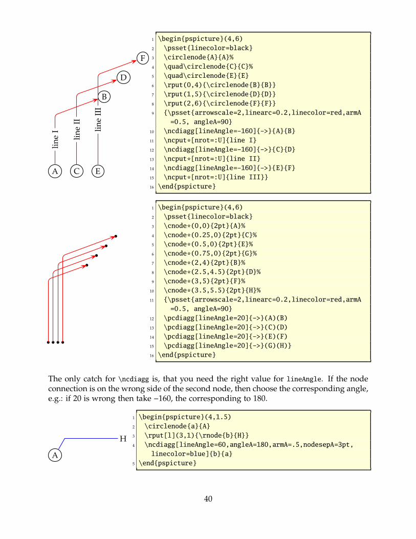
A C E

B

D

Fli

ne

I

lin

eII

lin

eII

I


2 \psset{linecolor=black}

3 \circlenode{A}{A}%

4 \quad\circlenode{C}{C}%

5 \quad\circlenode{E}{E}


7 \rput(1,5){\circlenode{D}{D}}

8 \rput(2,6){\circlenode{F}{F}}

9 {\psset{arrowscale=2,linearc=0.2,linecolor=red,armA

=0.5, angleA=90}

10 \ncdiagg[lineAngle=160]{>}{A}{B}

11 \ncput*[nrot=:U]{line I}

12 \ncdiagg[lineAngle=160]{>}{C}{D}

13 \ncput*[nrot=:U]{line II}

14 \ncdiagg[lineAngle=160]{>}{E}{F}

15 \ncput*[nrot=:U]{line III}}

16 \end{pspicture}



3 \cnode*(0,0){2pt}{A}%

4 \cnode*(0.25,0){2pt}{C}%

5 \cnode*(0.5,0){2pt}{E}%

6 \cnode*(0.75,0){2pt}{G}%

7 \cnode*(2,4){2pt}{B}%

8 \cnode*(2.5,4.5){2pt}{D}%

9 \cnode*(3,5){2pt}{F}%

10 \cnode*(3.5,5.5){2pt}{H}%

11 {\psset{arrowscale=2,linearc=0.2,linecolor=red,armA

=0.5, angleA=90}

12 \pcdiagg[lineAngle=20]{>}(A)(B)

13 \pcdiagg[lineAngle=20]{>}(C)(D)

14 \pcdiagg[lineAngle=20]{>}(E)(F)

15 \pcdiagg[lineAngle=20]{>}(G)(H)}

16 \end{pspicture}

The only catch for \ncdiagg is, that you need the right value for lineAngle. If the nodeconnection is on the wrong side of the second node, then choose the corresponding angle,e.g.: if 20 is wrong then take −160, the corresponding to 180.

A

H


2 \circlenode{a}{A}

3 \rput[l](3,1){\rnode{b}{H}}

4 \ncdiagg[lineAngle=60,angleA=180,armA=.5,nodesepA=3pt,

linecolor=blue]{b}{a}

5 \end{pspicture}

40

A

H


2 \circlenode{a}{A}


4 \ncdiagg[lineAngle=60,armA=.5,nodesepB=3pt,linecolor=blue

]{a}{b}

5 \end{pspicture}

A

H


2 \circlenode{a}{A}


4 \ncdiagg[lineAngle=120,armA=.5,nodesepB=3pt,linecolor=

blue]{a}{b}

5 \end{pspicture}

12 \ncbarr

This has the same behaviour as ncbar, but has 5 segments and all are horizontal ones.This is the reason why angleA must be 0 or alternative 180. All other values are set to 0by the macro. The intermediate horizontal line is symmetrical to the distance of the twonodes.

X

Y

1 \psset{arrowscale=2}%

2 \circlenode{X}{X}\\[1cm]

3 \circlenode{Y}{Y}

4 \ncbarr[angleA=0,arrows=>,arrowscale=2]{X}{Y}

Xxxxx

Yyyy


2 \ovalnode{X}{Xxxxx}\\[1cm]

3 \circlenode{Y}{Yyyy}

4 \ncbarr[angleA=180,arrows=>,arrowscale=2,linecolor=red]{X}{Y

}

Xxxxx

Yyyy


2 \ovalnode{X}{Xxxxx}\\[1cm]

3 \circlenode{Y}{Yyyy}

4 \ncbarr[angleA=20,arm=1cm,arrows=>,arrowscale=2]{X}{Y}

41

13 \psRelNode

With this macro it is possible to put a node relative to a given line. Parameter are theangle and the length factor:

\psRelNode(<P0>)(<P1>){<length factor>}{<end node name>}

\psRelLine[<options>](<P0>)(<P1>){<length factor>}{<end node name>}

The length factor depends to the distance of P0P1 and the end node name must be a validnodename and shouldn’t contain any of the special PostScript characters. There are twovalid options:

name default meaning

angle 0 angle between the given line P0P1 and the new one P0PendNode

trueAngle false defines whether the angle depends to the seen line or to themathematical one, which respect the scaling factors xunit andyunit.

0

30

60

90

120150

180

210

240

270

300 330


2 \psgrid[gridwidth=0pt,gridcolor=gray,

gridlabels=0pt,subgriddiv=2]

3 \pnode(3,3){A}\pnode(4,2){B}

4 \psline[nodesep=3,linewidth=0.5pt](A)(B)

5 \multido{\iA=0+30}{12}{%

6 \psRelNode[angle=\iA](A)(B){2}{C}%

7 \qdisk(C){2pt}

8 \uput[0](C){\iA}}

9 \end{pspicture}

14 \psRelLine

With this macro it is possible to plot lines relative to a given one. Parameter are the angleand the length factor:

\psRelLine(<P0>)(<P1>){<length factor>}{<end node name>}

\psRelLine{<arrows>}(<P0>)(<P1>){<length factor>}{<end node name>}

\psRelLine[<options>](<P0>)(<P1>){<length factor>}{<end node name>}

\psRelLine[<options>]{<arrows>}(<P0>)(<P1>){<length factor>}{<end node name>}

The length factor depends to the distance of P0P1 and the end node name must be a validnodename and shouldn’t contain any of the special PostScript characters. There are twovalid options which are described in the forgoing section for \psRelNode.

42

The following two figures show the same, the first one with a scaling different to 1 : 1,this is the reason why the end points are on an ellipse and not on a circle like in thesecond figure.

-2 -1 0 1 2 3-2

-1

0

1

21 \psset{yunit=2,xunit=1}


3 \psgrid[subgriddiv=2,subgriddots=10,gridcolor=

lightgray]


5 \psline[linecolor=red](A)(B)

6 \psRelLine[linecolor=blue,angle=30](1,0)(B){0.5}{

EndNode}

7 \qdisk(EndNode){2pt}

8 \psRelLine[linecolor=blue,angle=30](A)(B){0.5}{

EndNode}


10 \psRelLine[linecolor=magenta,angle=90](1,0)(3,2)

{0.5}{EndNode}


12 \psRelLine[linecolor=magenta,angle=90](A)(B){0.5}{

EndNode}


14 \end{pspicture}

-2 -1 0 1 2 3-2

-1

0

1

2


2 \psgrid[subgriddiv=2,subgriddots=10,gridcolor=

lightgray]



5 \psarc[linestyle=dashed](A){2.23}{90}{135}

6 \psRelLine[linecolor=blue,angle=30](1,0)(B){0.5}{

EndNode}


8 \psRelLine[linecolor=blue,angle=30](A)(B){0.5}{

EndNode}


10 \psRelLine[linecolor=magenta,angle=90](1,0)(3,2)

{0.5}{EndNode}


12 \psRelLine[linecolor=magenta,angle=90](A)(B){0.5}{

EndNode}


14 \end{pspicture}

The following figure has also a different scaling, but has set the option trueAngle, allangles depends to what "you see".

43

-3 -2 -1 0 1 2 3-1

0

1

2


2 \begin{pspicture}(3,1)(3,2)\psgrid[

subgridcolor=lightgray]



5 \psarc(A){2.83}{45}{135}

6 \psRelLine[linecolor=blue,angle=30,trueAngle](

A)(B){0.5}{EndNode}


8 \psRelLine[linecolor=blue,angle=30,trueAngle

](A)(B){0.5}{EndNode}


10 \psRelLine[linecolor=magenta,angle=90,

trueAngle](A)(B){0.5}{EndNode}


12 \psRelLine[linecolor=magenta,angle=90,

trueAngle](A)(B){0.5}{EndNode}


14 \end{pspicture}

Two examples with using \multido to show the behaviour of the options trueAngle andangle.

-1 0 1 2 30

1

2





4 \psline[linecolor=red](A)(3,2)

5 \multido{\iA=0+10}{36}{%

6 \psRelLine[linecolor=blue,angle=\iA](

B)(A){0.5}{EndNode}


8 }

9 \end{pspicture}

44

-1 0 1 2 30

1

2





4 \psline[linecolor=red](A)(3,2)

5 \multido{\iA=0+10}{36}{%

6 \psRelLine[linecolor=magenta,angle=\

iA,trueAngle]{>}(B)(A){0.5}{

EndNode}

7 }

8 \end{pspicture}

Anstr"omrichtung v∞

FH

FV FR

FN

FT

1 \psset{xunit=0.75\linewidth,yunit=0.75\linewidth,trueAngle}%

2 \end{center}

3 \begin{pspicture}(1,0.6)%\psgrid

4 \pnode(.3,.35){Vk} \pnode(.375,.35){D} \pnode(0,.4){DST1} \pnode(1,.18){DST2}

5 \pnode(0,.1){A1} \pnode(1,.31){A1}

6 { \psset{linewidth=.02,linestyle=dashed,linecolor=gray}%

7 \pcline(DST1)(DST2) % < Druckseitentangente

8 \pcline(A2)(A1) % < Anstr"omrichtung

9 \lput*{:U}{\small Anstr"omrichtung $v_{\infty}$} }%

10 \psIntersectionPoint(A1)(A2)(DST1)(DST2){Hk}

11 \pscurve(Hk)(.4,.38)(Vk)(.36,.33)(.5,.32)(Hk)

12 \psParallelLine[linecolor=red!75!green,arrows=>,arrowscale=2](Vk)(Hk)(D){.1}{

FtE}

45

13 \psRelLine[linecolor=red!75!green,arrows=>,arrowscale=2,angle=90](D)(FtE){4}{

Fn}% why "4"?

14 \psParallelLine[linestyle=dashed](D)(FtE)(Fn){.1}{Fnr1}

15 \psRelLine[linestyle=dashed,angle=90](FtE)(D){4}{Fnr2} % why "4"?

16 \psline[linewidth=1.5pt,arrows=>,arrowscale=2](D)(Fnr2)

17 \psIntersectionPoint(D)([nodesep=2]D)(Fnr1)([offset=4]Fnr1){Fh}

18 \psIntersectionPoint(D)([offset=2]D)(Fnr1)([nodesep=4]Fnr1){Fv}

19 \psline[linecolor=blue,arrows=>,arrowscale=2](D)(Fh)

20 \psline[linecolor=blue,arrows=>,arrowscale=2](D)(Fv)

21 \psline[linestyle=dotted](Fh)(Fnr1) \psline[linestyle=dotted](Fv)(Fnr1)

22 \uput{.1}[0](Fh){\blue $F_{H}$} \uput{.1}[180](Fv){\blue $F_{V}$}

23 \uput{.1}[45](Fnr1){$F_{R}$} \uput{.1}[90](Fn){\color{red!75!green}$F_{N}

$}

24 \uput{.25}[90](FtE){\color{red!75!green}$F_{T}$}

25 \end{pspicture}

15 \psParallelLine

With this macro it is possible to plot lines relative to a given one, which is parallel. Thereis no special parameter here.

\psParallelLine(<P0>)(<P1>)(<P2>){<length>}{<end node name>}

\psParallelLine{<arrows>}(<P0>)(<P1>)(<P2>){<length>}{<end node name>}

\psParallelLine[<options>](<P0>)(<P1>)(<P2>){<length>}{<end node name>}

\psParallelLine[<options>]{<arrows>}(<P0>)(<P1>)(<P2>){<length>}{<end node name>}

The line starts at P2, is parallel to P0P1 and the length of this parallel line depends to thelength factor. The end node name must be a valid nodename and shouldn’t contain anyof the special PostScript characters.

46

-4

-3

-2

-1

0

1

2

3

1 \begin{pspicture*}(5,4)(5,3.5)


3 \pnode(2,2){FF}\qdisk(FF){1.5pt}

4 \pnode(5,5){A}\pnode(0,0){O}

5 \multido{\nCountA=2.4+0.4}{9}{%

6 \psParallelLine[linecolor=red](O)(

A)(0,\nCountA){9}{P1}

7 \psline[linecolor=red](0,\nCountA)

(FF)

8 \psRelLine[linecolor=red](0,\

nCountA)(FF){9}{P2}

9 }

10 \psline[linecolor=blue](A)(FF)

11 \psRelLine[linecolor=blue](A)(FF)

{5}{END1}

12 \psline[linewidth=2pt,arrows

=>](2,0)(FF)

13 \end{pspicture*}

16 \psIntersectionPoint

This macro calculates the intersection point of two lines, given by the four coordinates.There is no special parameter here.

\psIntersectionPoint(<P0>)(<P1>)(<P2>)(<P3>){<node name>}

1234

−1−2−3−4

1 2 3 4−1−2−3−4−5A

B

C

D

IP

1 \psset{unit=0.5cm}


3 \psaxes{>}(0,0)(5,4)(5,5)

4 \psline[linecolor=red,linewidth=2pt](5,1)(5,5)

5 \psline[linecolor=blue,linewidth=2pt](5,3)(5,4)

6 \qdisk(5,1){3pt}\uput[90](5,1){A}

7 \qdisk(5,5){3pt}\uput[90](5,5){B}

8 \qdisk(5,3){3pt}\uput[90](5,3){C}

9 \qdisk(5,4){3pt}\uput[90](5,4){D}

10 \psIntersectionPoint(5,1)(5,5)(5,3)(5,4){IP}

11 \qdisk(IP){5pt}\uput{0.3}[90](IP){IP}

12 \psline[linestyle=dashed](IP|0,0)(IP)(0,0|IP)

13 \end{pspicture}

47

17 \psLNode and \psLCNode

\psLNode interpolates the Line AB by the given value and sets a node at this point. Thesyntax is

\psLNode(P1)(P2){value}{Node name}

0 1 2 3 4 50

1

2

3

4




4 \psline{oo}(1,1)(5,5)

5 \psLNode(1,1)(5,5){0.75}{PI}

6 \qdisk(PI){4pt}

7 \psset{linecolor=blue}

8 \psline{oo}(4,3)(2,5)

9 \psLNode(4,3)(2,5){0.5}{PII}

10 \qdisk(PII){4pt}

11 \end{pspicture}

The \psLCNode macro builds the linear combination of the two given vectors and storesthe end of the new vector as a node. All vectors start at (0, 0), so a \rput maybe appro-priate. The syntax is

\psLCNode(P1){value 1}(P2){value 2}{Node name}

0 1 2 3 4 50

1

2

3

4




4 \psline[linestyle=dashed]{>}(3,1.5)

5 \psline[linestyle=dashed]{>}(0.375,1.5)


7 \psline{>}(2,1)\psline{>}(0.5,2)

8 \psLCNode(2,1){1.5}(0.5,2){0.75}{PI}

9 \psline[linewidth=2pt]{>}(PI)


11 \psline[linestyle=dashed](3,1.5)(PI)

12 \psline[linestyle=dashed](0.375,1.5)(PI)

13 \end{pspicture}

48

18 \nlput and \psLDNode

\ncput allows to set a label relative to the first node of the last node connection. With\nlput this can be done absolute to a given node. The syntax is different to the othernode connection makros. It uses internally the macro \psLDNode which places a nodeabsolute to two given points, starting from the first one.

\nlput[options](A)(B){distance}{text}

\psLDNode[options](A)(B){distance}{node name}

Test

Test TestTest


2 \pnode(0,0){A}

3 \pnode(5,2){B}

4 \ncline{A}{B}

5 \psLDNode(A)(B){1.5cm}{KN}\qdisk(KN){2pt}

6 \nlput[nrot=:U](A)(B){1cm}{Test}

7 \nlput[nrot=:D](A)(B){2cm}{Test}

8 \nlput[nrot=:U](A)(B){3cm}{Test}

9 \nlput(A)(B){4cm}{Test}

10 \end{pspicture}

49

Part III

pstplot

19 New options

The option tickstyle=full|top|bottom is no more working in the pstricksadd package,because everything can be set by the ticksize option. When using the comma or trigLabelsoption, the macros \pshlabel and \psvlabel shouldn’t be redefined, because the packagedoes it itself in these cases.

Table 2: All new parameters for pstplot

Name Type DefaultlabelFontSize <fontsize macro> {}

algebraic false|true false

comma false|true false

xAxis false|true true

yAxis false|true true

xyAxes false|true true

xDecimals <number> or empty {}

yDecimals <number> or empty {}

xyDecimals <number> or empty {}

ticks <all|x|y|none> all

labels <all|x|y|none> all

subticks <number> 0

xsubticks <number> 0

ysubticks <number> 0

ticksize <length [length]> 4pt 4pt

subticksize <number> 0.75

tickwidth <length> 0.5\pslinewidth

subtickwidth <length> 0.25\pslinewidth

tickcolor <color> black

xtickcolor <color> black

ytickcolor <color> black

subtickcolor <color> darkgray

xsubtickcolor <color> darkgray

ysubtickcolor <color> darkgray

ticklinestyle solid | dashed | dotted | none solid

subticklinestyle solid | dashed | dotted | none solid

xlabelFactor <anything> {\ empty}

ylabelFactor <anything> {\ empty}

xlogBase <number> or empty {}

ylogBase <number> or empty {}

50

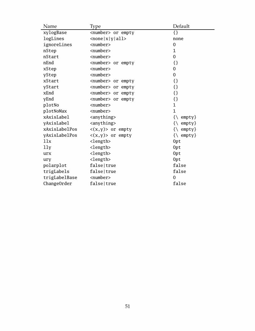
Name Type DefaultxylogBase <number> or empty {}

logLines <none|x|y|all> none

ignoreLines <number> 0

nStep <number> 1

nStart <number> 0

nEnd <number> or empty {}

xStep <number> 0

yStep <number> 0

xStart <number> or empty {}

yStart <number> or empty {}

xEnd <number> or empty {}

yEnd <number> or empty {}

plotNo <number> 1

plotNoMax <number> 1

xAxisLabel <anything> {\ empty}

yAxisLabel <anything> {\ empty}

xAxisLabelPos <(x,y)> or empty {\ empty}

yAxisLabelPos <(x,y)> or empty {\ empty}

llx <length> 0pt

lly <length> 0pt

urx <length> 0pt

ury <length> 0pt

polarplot false|true false

trigLabels false|true false

trigLabelBase <number> 0

ChangeOrder false|true false

51

19.1 Changing the label font size with labelFontSize

This option sets the horizontal and vertical font size for the labels. It will be overwrittenwhen another package or a user defines

1 \def\pshlabel#1{...}

2 \def\psvlabel#1{...}

0

1

2

0 1 2 3 4

0

1

2

0 1 2 3 4

0

1

2

0 1 2 3 4

0

1

2

0 1 2 3 4

1 \begin{pspicture}(0.25,0.25)(5,2.25)

2 \psaxes{>}(5,2.25)

3 \end{pspicture}\\[20pt]

4 \begin{pspicture}(0.25,0.25)(5,2.25)

5 \psaxes[labelFontSize=\small]{>}(5,2.25)


7 \begin{pspicture}(0.25,0.25)(5,2.25)

8 \psaxes[labelFontSize=\footnotesize]{>}(5,2.25)


10 \begin{pspicture}(0.25,0.25)(5,2.25)

11 \psaxes[labelFontSize=\tiny]{>}(5,2.25)

12 \end{pspicture}%

52

19.2 algebraic1

By default the function of \psplot has to be described in Reversed Polish Notation. Theoption algebraic allows to do this in the common algebraic notation. E.g.:

RPN algebraicx ln ln(x)

x cos 2.71 x neg 10 div exp mul cos(x)*2.71^(x/10)

1 x div cos 4 mul 4*cos(1/x)

t cos t sin cos(t)|sin(t)

Setting the option algebraic to true, allow the user to describe all expression to be writtenin the classical algebraic notation (infix notation). The four arithmetic operarions areobviously defined +*/, and also the exponential operator ^. The natural priorities areused : 3+ 4× 55 = 3 + (4× (55)), and by default the computation is done from left to right.The following functions are defined :

sin, cos, tan, acos, asin in radianslog, lnceiling, floor, truncate, roundsqrt square rootabs absolute valuefact for the factorialSum for building sumsIfTE for an easy case structure

These options can be used with all plot macros.

Using the option algebraic implies that all angles have to be used in the radian unit!

For the \parametricplot the two parts must be divided by the | character:

1 \begin{pspicture}(0.5,0.5)(0.5,0.5)

2 \parametricplot[algebraic,linecolor=red]{3.14}{3.14}{cos(t)|sin(t)}

3 \end{pspicture}

1This part is adapted from the package psteqdf, written by Dominique Rodriguez.

53

0

1

2

3

4

5

0 1 2 3 4 5 6 7 8 9 10 11 12 13 14 15 16 17 18 19 20x

y

�

�

�

�

�

�

�

�

�

��

�

�

�

�

�

�

�

�

�

�

�

�

�

��

�

�

�

�

�

�

�

�

�

�

�

�

��

�

�

�

�

�

�

�

�

�

�

�

�

��

�

�

�

�

�

�

�

�

�

�

�

�

��

�

�

�

�

�

�

�

�

�

�

�

�

�

��

�

�

�

�

�

�

�

�

�

�

1 \psset{lly=0.5cm}

2 \psgraph(10,3)(10,2){\linewidth}{6cm}

3 \psset{algebraic=true, plotpoints=101}

4 \psplot[linecolor=yellow, linewidth=4\pslinewidth]{10}{10}{2*sin(x)}%

5 \psplot[linecolor=red, showpoints=true]{10}{10}{2*sin(x)}

6 \endpsgraph

0

1

2

3

4

5

6

7

8

0 1 2 3 4 5 6 7 8 9 10 11 12 13 14 15 16 17 18x

y�

�

�

�

�

�

�

�

� �

�

�

�

�

�

�

��

�

�

�

�

�

��

�

�

�

�

��

� � ��

�

�

��

� � � ��

��

��

1 \psset{lly=0.5cm}

2 \psgraph(0,5)(18,3){15cm}{5cm}

3 \psset{algebraic,plotpoints=501}

4 \psplot[linecolor=yellow, linewidth=4\pslinewidth]{0.01}{18}{ln(x)}%

5 \psplot[linecolor=red]{0.01}{18}{ln(x)}

6 \psplot[linecolor=yellow,linewidth=4\pslinewidth]{0}{18}{3*cos(x)*2.71^(x/10)

}

7 \psplot[linecolor=blue,showpoints=true,plotpoints=51]{0}{18}{3*cos(x)*2.71^(x

/10)}

8 \endpsgraph

54

19.2.1 Using the Sum function

Syntax: Sum(<index name>,<start>,<step>,<end>,<function>)

Let’s plot the first development of cosine with polynomials:+∞∑

n=0

(−1)nx2n

n!.

1

−1

1 2 3 4 5 6 7−1−2−3−4−5−6−7

1 \psset{algebraic=true,plotpoints=501, yunit=3}

2 \def\getColor#1{\ifcase#1 black\or red\or magenta\or yellow\or green\or Orange\

or blue\or

3 DarkOrchid\or BrickRed\or Rhodamine\or OliveGreen\fi}


5 \psclip{\psframe(7,1.5)(7,1.5)}

6 \psplot{7}{7}{cos(x)}

7 \multido{\n=1+1}{10}{%

8 \psplot[linewidth=1pt,linecolor=\getColor{\n}]{7}{7}{%

9 Sum(ijk,0,1,\n,(1)^ijk*x^(2*ijk)/fact(2*ijk))}}

10 \endpsclip

11 \psaxes(0,0)(7,1.5)(7,1.5)

12 \end{pspicture}

55

19.2.2 Using the IfTE function

Syntax: IfTE(<condition>,<true part>,<false part>)

Nesting of several IfTE are possible and seen in the following examples. A classicalexample is a piece wise linear function.

-8 -7 -6 -5 -4 -3 -2 -1 0 1 2 3 4 5 6 7 8-2

-1

0

1

2

3

4

5

6

1 \begin{pspicture}(7.5,2.5)(7.5,6)\psgrid[subgriddiv=1,gridcolor=lightgray]

2 \psset{algebraic=true, plotpoints=21,linewidth=2pt}

3 \psplot[linecolor=blue]{7.5}{7.5}{IfTE(x<6,8+x,IfTE(x<0,x/3,IfTE(x<3,2*x,9

x)))}

4 \psplot[linecolor=red, plotpoints=101]{7.5}{7.5}{%

5 IfTE(2*x<2^2*sqrt(9),7+x,IfTE(x<0,x^2/181,IfTE(x<3,2*x^2/31,8x)))}%

6 \end{pspicture}

When you program a piece-wise defined function you must take care that a plottingpoint must be put on each point where the description changes. Use showpoints=true tosee what’s going on, when there is a problem. You are on the save side, when you choosea big number for plotpoints.

56

-8 -7 -6 -5 -4 -3 -2 -1 0 1 2 3 4 5 6 7 8-8

-7

-6

-5

-4

-3

-2

-1

0

1

2

3

4

5

6

7

8

1 \begin{pspicture}[showgrid=true](8,8)(8,8)

2 \psset{plotpoints=1000,linewidth=1pt}

3 \psplot[algebraic, linecolor=yellow]{8}{8}{rand/(2^311)+x}

4 \psplot[algebraic]{8}{8}{ceiling(x)}

5 \psplot[algebraic, linecolor=red]{8}{8}{floor(x)}

6 \psplot[algebraic, linecolor=blue]{8}{8}{round(x)}

7 \psplot[algebraic, linecolor=green]{8}{8}{truncate(x)}

8 \psplot[algebraic, linecolor=cyan]{8}{8}{div(mul(4,x),7)}

9 \psplot[algebraic, linecolor=gray]{8}{8}{abs(x)+abs(x3)abs(55*x/7)}

10 \psplot[algebraic, linecolor=gray]{8}{8}{abs(3*cos(x)+1)}

11 \psplot[algebraic, linecolor=magenta]{8}{8}{floor(8*cos(x))}

12 \end{pspicture}

57

19.3 comma

Syntax:

comma=false|true

Setting this option to true gives labels with a comma as a decimal separator instead ofthe dot. comma and comma=true is the same.

00,51,01,52,02,53,03,54,04,5

0 1,5 3,0 4,5

1 \begin{pspicture}(0.5,0.5)(5,5.5)

2 \psaxes[Dx=1.5,Dy=0.5,comma]{>}(5,5)

3 \psplot[linecolor=red,linewidth=3pt]{0}{4.5}%

4 {x 180 mul 1.52 div cos 2 mul 2.5 add}

5 \psline[linestyle=dashed](0,2.5)(4.5,2.5)

6 \end{pspicture}

19.4 xyAxes, xAxis and yAxis

Syntax:

xyAxes=true|false

xAxis=true|false

yAxis=true|false

Sometimes there is only a need for one axis with ticks. In this case you can set one ofthe following options to false. The xyAxes makes only sense, when you want to set both,x and y to true with only one command again to the default, because with xyAxes=false

you get nothing with the psaxes macro.

58

0 1 2 3 4

0

1

2

3

4

0

1

2

3

4

0

1

2

3

4

0

1

2

3

4


2 \psaxes[yAxis=false,linecolor=blue

]{>}(0,0.5)(5,0.5)

3 \end{pspicture}


5 \psaxes[xAxis=false,linecolor=red

]{>}(0.5,0)(0.5,5)

6 \end{pspicture}



]{>}(0.5,0)(0.5,5)

9 \end{pspicture}\hspace{2em}


11 \psaxes[xAxis=false,linecolor=red,

labelsep=20pt]{>}(0.5,0)(0.5,5)

12 \end{pspicture}%



]{>}(0.5,0)(0.501,5)

15 \end{pspicture}%

As seen in the example, a single y axis gets the labels on the right side. This can bechanged in two ways, first with the option labelsep and second with a very short andtherefore invisible x-axis (right example).

19.5 xyDecimals, xDecimals and yDecimals

Syntax:

xyDecimals=<number>

xDecimals=<any>

yDecimals=<any>

By default the labels of the axes get numbers with or without decimals, just dependingto the numbers. With these options ??Decimals it is possible to determine the decimals,where the option xyDecimals sets this identical for both axes. The default setting {}

means, that you’ll get the standard behaviour.

0.00

1.00

2.00

3.00

0.00 1.00 2.00 3.00 4.00

1 \begin{pspicture}(1.5,0.5)(5,3.75)

2 \psaxes[xyDecimals=2]{>}(0,0)(4.5,3.5)

3 \end{pspicture}

59

0,0

100,0

200,0

300,0

400,0

500,0

−100,0

0,250 0,500 0,750 1,000 1,250

1 \psset{xunit=10cm,yunit=0.01cm,

labelFontSize=\footnotesize}

2 \begin{pspicture}(0.3,150)

(1.5,550.0)

3 \psaxes[Dx=0.25,Dy=100,ticksize=4pt

0,comma=true,%

4 xDecimals=3,yDecimals=1]{>}(0,0)

(0,100)(1.4,520)

5 \end{pspicture}

19.6 ticks

Syntax:

ticks=all|x|y|none

This option is also already in the pstplot package and only mentioned here for somecompletness.

1

−1

1−1

1 \psset{ticksize=6pt}


3 \psaxes[ticks=all,subticks=5]{>}(0,0)(1,1)(2,2)

4 \end{pspicture}

1

−1


2 \psaxes[ticks=y,subticks=5]{>}(0,0)(1,1)(2,2)

3 \end{pspicture}

1 2


2 \psaxes[ticks=x,subticks=5]{>}(0,0)(2,2)(1,1)

3 \end{pspicture}

60


2 \psaxes[ticks=none,subticks=5]{>}(0,0)(2,2)(1,1)

3 \end{pspicture}

19.7 labels

Syntax:

labels=all|x|y|none

This option is also already in the pstplot package and only mentioned here for somecompletness.

1

−1

1−1



3 \psaxes[labels=all,subticks=5]{>}(0,0)(1,1)(2,2)

4 \end{pspicture}

1

−1


2 \psaxes[labels=y,subticks=5]{>}(0,0)(1,1)(2,2)

3 \end{pspicture}

1 2


2 \psaxes[labels=x,subticks=5]{>}(0,0)(2,2)(1,1)

3 \end{pspicture}


2 \psaxes[labels=none,subticks=5]{>}(0,0)(2,2)(1,1)

3 \end{pspicture}

61

19.8 ticksize, xticksize, yticksize

With this new option the recent tickstyle option of pstplot is obsolete and no moresupported by pstricksadd.

Syntax:

ticksize=value[unit]

ticksize=value[unit] value[unit]

xticksize=value[unit]

xticksize=value[unit] value[unit]

yticksize=value[unit]

yticksize=value[unit] value[unit]

ticksize sets both values. The first one is left/below and the optional second one isright/above of the coordinate axis. The old setting tickstyle=bottom is now easy torealize, e.g.: ticksize=6pt 0, or vice versa, if the coordinates are set from positive tonegative values.

1

2

3

−1

1 2 3−1



3 \psaxes[ticksize=0.5cm]{>}(0,0)(1.5,1.5)

(4,3.5)

4 \end{pspicture}

1

2

3

−11 2 3−1



3 \psaxes[xticksize=10pt 0,yticksize=0 10pt

]{>}(0,0)(1.5,1.5)(4,3.5)

4 \end{pspicture}

A grid is also possible by setting the values to the max/min coordinates.

62

1

2

3

4

1 2 3 4


2 \begin{pspicture}(.5,.5)(5,4.5)

3 \psaxes[ticklinestyle=dashed,ticksize=0 4cm

]{>}(0,0)(.5,.5)(5,4.5)

4 \end{pspicture}

19.9 subticks

Syntax:

subticks=<number>

By default subticks cannot have labels.

1

−1

1−1



3 \psaxes[ticks=all,subticks=5]{>}(0,0)(1,1)(2,2)

4 \end{pspicture}

1

−1


2 \psaxes[ticks=y,subticks=5]{>}(0,0)(1,1)(2,2)

3 \end{pspicture}

1 2


2 \psaxes[ticks=x,subticks=5]{>}(0,0)(2,2)(1,1)

3 \end{pspicture}


2 \psaxes[ticks=none,subticks=5]{>}(0,0)(2,2)(1,1)

3 \end{pspicture}

63

19.10 subticksize, xsubticksize, ysubticksize

Syntax:

subticksize=value

xsubticksize=value

ysubticksize=value

subticksize sets both values, which are relative to the ticksize length and can have anynumber. 1 sets it to the same length as the main ticks.

−1

−2

−3

−4

1 2 3−11 \psset{yunit=1.5cm,xunit=3cm}

2 \begin{pspicture}(1.25,4.75)(3.25,.75)

3 \psaxes[xticksize=4.5 0.5,ticklinestyle=dashed,subticks=5,xsubticksize=1,%

4 ysubticksize=0.75,xsubticklinestyle=dotted,xsubtickwidth=1pt,

5 subtickcolor=gray]{>}(0,0)(1,4)(3.25,0.5)

6 \end{pspicture}

64

19.11 tickcolor, subtickcolor

Syntax:

tickcolor=<color>

xtickcolor=<color>

ytickcolor=<color>

subtickcolor=<color>

xsubtickcolor=<color>

ysubtickcolor=<color>

tickcolor and subtickcolor set both for the x- and the y-Axis.

0 1 2 3 4 5 6 7 8 9 10


2 \psaxes[labelsep=2pt,yAxis=false,labelFontSize=\footnotesize,%

3 labelsep=10pt,ticksize=0 10mm,subticks=10,subticksize=0.75,%

4 tickcolor=red,subtickcolor=blue,tickwidth=1pt,%

5 subtickwidth=0.5pt](10.01,0)

6 \end{pspicture}

5 6 7 8 9 10


2 \psaxes[labelsep=2pt,yAxis=false,labelFontSize=\

footnotesize,%

3 labelsep=5pt,ticksize=0 10mm,subticks=10,

subticksize=0.75,%

4 tickcolor=red,subtickcolor=blue,tickwidth=1pt,%

5 subtickwidth=0.5pt,Ox=5](5,0)(5,0)(10.01,0)

6 \end{pspicture}

19.12 ticklinestyle and subticklinestyle

Syntax:

ticklinestyle=solid|dashed|dotted|none

xticklinestyle=solid|dashed|dotted|none

yticklinestyle=solid|dashed|dotted|none

subticklinestyle=solid|dashed|dotted|none

xsubticklinestyle=solid|dashed|dotted|none

ysubticklinestyle=solid|dashed|dotted|none

ticklinestyle and subticklinestyle set both values for the x and y axis. The value none

doesn’t really makes sense, because it is the same to [sub]ticklines=0

65

100

101

0 1 2

1 \psset{unit=4cm}

2 \pspicture(0.15,0.15)(2.5,1)

3 \psaxes[axesstyle=frame,logLines=y,xticksize=0 1,xsubticksize=1,%

4 ylogBase=10,tickcolor=red,subtickcolor=blue,tickwidth=1pt,%

5 subticks=20,xsubticks=10,xticklinestyle=dashed,%

6 xsubticklinestyle=dashed](2.5,1)

7 \endpspicture

19.13 loglines

Syntax:

loglines=all|x|y

100

101

102

103

104

105

100 101 102 103 104 105

1 \pspicture(0,1)(5,5)

2 \psaxes[subticks=5,axesstyle=frame,xylogBase=10,

logLines=all](5,5)

3 \endpspicture

66

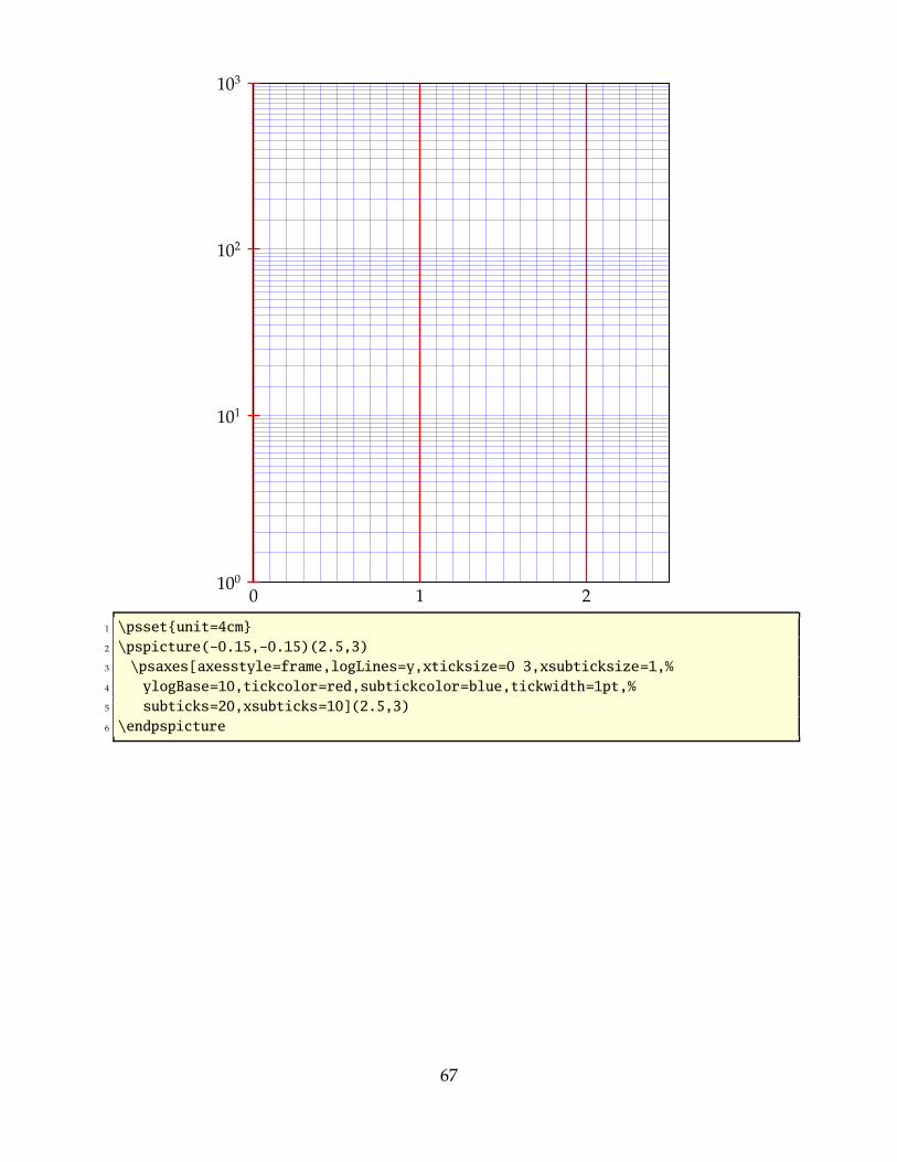
100

101

102

103

0 1 2

1 \psset{unit=4cm}

2 \pspicture(0.15,0.15)(2.5,3)

3 \psaxes[axesstyle=frame,logLines=y,xticksize=0 3,xsubticksize=1,%

4 ylogBase=10,tickcolor=red,subtickcolor=blue,tickwidth=1pt,%

5 subticks=20,xsubticks=10](2.5,3)

6 \endpspicture

67

0

0.5

1.0

100 101 102 103

1 \psset{unit=4}

2 \pspicture(0.5,0.3)(3,1.2)

3 \psaxes[axesstyle=frame,logLines=x,xlogBase=10,Dy=0.5,%

4 tickcolor=red,subtickcolor=blue,tickwidth=1pt,ysubticks=5,xsubticks=10](3,1)

5 \endpspicture

19.14 xylogBase, xlogBase and ylogBase

There are additional options xylogBase xlogBase | ylogBase| to get one or both axeswith logarithm labels. For an intervall of [10−3...102] choose a pstricks intervall of [-3,2].pstricks takes 0 as the origin of this axes, which is wrong if we want to have a logarithmaxes. With the options Oy and Ox we can set the origin to −3, so that the first label gets10−3. If this is not done by the user then pstricksadd does it by default. An alternativeis to set these parameters to empty values Ox={},Oy={}, in this case pstricksadd doesnothing.

19.14.1 xylogBase

This mode is in math also called double logarithm. It is a combination of the two forgoingmodes and the function is now y = logx and is shown in the following example.

68

10-3

10-2

10-1

100

101

102

103

100 101 102 103 104 105 106 x

y

y = logx

1 \begin{pspicture}(3.5,3.5)(3.5,3.5)

2 \psplot[linewidth=2pt,linecolor=red

]{0.001}{3}{x log}

3 \psaxes[xylogBase=10,Oy=3]{<>}(3,3)

(3.5,3.5)

4 \uput[90](3.5,3){x}

5 \uput[180](3,3.5){y}

6 \rput(2.5,1){$y=\log x$}

7 \end{pspicture}

19.14.2 ylogBase

The values for the psaxes y-coordinate are now the exponents to the base 10 and forthe right function to the base e: 10−3 . . . 101 which corresponds to the given y-intervall−3 . . . 1.5, where only integers as exponents are possible. These logarithm labels have noeffect to the internal used units. To draw the logarithm function we have to use the mathfunction

y = log{logx}y = ln{lnx}

with an drawing intervall of 1.001 . . .6.

100

101

102

103

104

0 1 2 3 4 5 6x

yy = logx 1 \begin{pspicture}(0.5,3.5)(6.5,1.5)

2 \psaxes[ylogBase=10]{<>}(0,3)(6.5,1.5)

3 \uput[90](6.5,3){x}

4 \uput[0](0,1.4){y}

5 \rput(5,1){$y=\log x$}

6 \psplot[linewidth=2pt,%

7 plotpoints=100,linecolor=red]{1.001}{6}{x

log log} % log(x)

8 \end{pspicture}

69

e0

e1

e2

e3

e4

0 1 2 3 4 5 6x

y

y = lnx1 \begin{pspicture}(0.5,3.5)(6.5,1.5)

2 \psplot[linewidth=2pt,plotpoints=100,

linecolor=red]%

3 {1.04}{6}{/ln {log 0.4343 div} def x ln

ln} % log(x)

4 \psaxes[ylogBase=e]{<>}(0,3)(6.5,1.5)

5 \uput[90](6.5,3){x}

6 \uput[0](0,1.5){y}

7 \rput(5,1){$y=\ln x$}

8 \end{pspicture}

102

103

104

0 1 2 3 4 5 6

1 \begin{pspicture}(0.5,1.75)(6.5,4.5)

2 \psaxes[ylogBase=10,Oy=2]{<>}(0,2)(0,2)

(6.5,4.5)

3 \end{pspicture}

100

101

102

103

104

0 1 2 3 4 5 6

1 \begin{pspicture}(0.5,0.25)(6.5,4.5)

2 \psplot{0}{6}{x x cos add log} %

x + cox(x)

3 \psplot[linecolor=red]{0}{6}{x 3 exp x

cos add log} % x^3 + cos(x)

4 \psplot[linecolor=cyan]{0}{6}{x 5 exp x


5 \psaxes[ylogBase=10]{<>}(6.5,4.5)

6 \end{pspicture}

100

101

102

103

104

105

0 1 2 3 4 5 6

1 \begin{pspicture}(0.5,1.25)(6.5,4.5)

2 \psplot{0}{6}{x x cos add log} % x

+ cox(x)

3 \psplot[linecolor=red]{0}{6}{x 3 exp x cos

add log} % x^3 + cos(x)

4 \psplot[linecolor=cyan]{0}{6}{x 5 exp x


5 \psaxes[ylogBase=10]{<>}(0,1)(0,1)

(6.5,4.5)

6 \end{pspicture}

70

102

103

104

3 4 5 6

1 \begin{pspicture}(2.5,1.75)(6.5,4.5)

2 \psplot[linecolor=cyan]{3}{6}{x 5 exp x cos add log} % x

^5 + cos(x)

3 \psaxes[ylogBase=10,Ox=3,Oy=2]{>}(3,2)(3,2)(6.5,4.5)

4 \end{pspicture}

19.14.3 xlogBase

Now we have to use the easy math function y = x because the x axis is still logx.

10-3

10-2

10-1

100

101

102

103

−3 −2 −1 0 1 2 3x

y

y = logx

y = lnx

1 \begin{pspicture}(3.5,3.5)(3.5,3.5)

2 \psplot[linewidth=2pt,linecolor=red

]{3}{3}{x} % log(x)

3 \psplot[linewidth=2pt,linecolor=blue

]{1.3}{1.5}{x 0.4343 div} % ln(x)

4 \psaxes[ylogBase=10,Oy=3,Ox

=3]{>}(3,3)(3.5,3.5)

5 \uput[90](3.5,3){x}

6 \uput[180](3,3.5){y}

7 \rput(2.5,1){$y=\log x$}

8 \rput[lb](0,1){$y=\ln x$}

9 \end{pspicture}

x

y y = sinx

−1

0

1

100 101 102 103 104 105

71

1 \psset{yunit=3cm,xunit=2cm}

2 \begin{pspicture}(1.25,1.25)(4.25,1.5)

3 \uput[90](4.25,1){x}

4 \uput[0](1,1){y}

5 \rput(0,1){$y=\sin x$}

6 \psplot[linewidth=2pt,plotpoints=5000,linecolor=red]{1}{3.5}{10 x exp sin }

7 \psaxes[xlogBase=10,Oy=1]{>}(1,1)(4.25,1.25)

8 \end{pspicture}

1

2

−1

−2

101 102 10310-110-210-3

1 \begin{pspicture}(3.5,2.5)(3.5,2.5)

2 \psaxes[xlogBase=10]{>}(0,0)(3.5,2.5)

(3.5,2.5)

3 \psplot{2.5}{2.5}{10 x exp log}

4 \end{pspicture}

1

2

−1

−2

101 102 10310-110-210-3

1 \begin{pspicture}(3.5,2.5)(3.5,2.5)

2 \psaxes[xlogBase=10,Ox={},Oy={}]{>}(0,0)

(3.5,2.5)(3.5,2.5)

3 \psplot{2.5}{2.5}{10 x exp log}

4 \end{pspicture}

19.14.4 No logstyle (xylogBase={})

This is only a demonstration that the default option logBase={} still works ... :-)

1

2

0 1 2 3−1−2−3x

y

y = logx

1 \begin{pspicture}(3.5,0.5)(3.5,2.5)

2 \psplot[linewidth=2pt,linecolor=red,

xylogBase={}]{0.5}{3}{x log} % log(x)

3 \psaxes{>}(0,0)(3.5,0)(3.5,2.5)

4 \uput[90](3.5,0){x}

5 \uput[180](0,2.5){y}

6 \rput(2.5,1){$y=\log x$}

7 \end{pspicture}

72

19.15 subticks, tickwidth and subtickwidth

0 1 2 3 4−1−2−3−4−5

0−1−2−3−4 1 2 3 4 5

0 1 2 3 4−1−2−3−4−5

0 1 2 3 4−1−2−3−4−5

0−1−2−3−4 1 2 3 4 5

0−1−2−3−4 1 2 3 4 5

0 1 2 3 4−1−2−3−4−5

0−1−2−3−4 1 2 3 4 5

0 1 2 3 4−1−2−3−4−5

0−1−2−3−4 1 2 3 4 5


2 \psaxes[labelsep=2pt,yAxis=false,subticks=8]{>}(0,0)(5,1)(5,1)\\[1cm]

3 \psaxes[yAxis=false,subticks=4,ticksize=4pt 0]{>}(0,0)(5,1)(5,1)\\

4 \psaxes[yAxis=false,subticks=4,ticksize=10pt 0]{>}(0,0)(5,5)(5,5)\\[1cm]

5 \psaxes[yAxis=false,subticks=10,ticksize=0 10pt,labelsep=15pt]{>}(0,0)(5,5)(5,5)\\[1

cm]

6 \psaxes[yAxis=false,subticks=4,ticksize=0 10pt,labelsep=15pt]{>}(0,0)(5,5)(5,5)\\[1cm

]

7 \psaxes[yAxis=false,subticks=4,ticksize=0 10pt]{>}(0,0)(5,5)(5,5)\\[0.25cm]

8 \psaxes[yAxis=false,subticks=0]{>}(0,0)(5,5)(5,5)\\[1cm]

9 \psaxes[yAxis=false,subticks=0,tickcolor=red,linecolor=blue]{>}(0,0)(5,5)(5,5)\\

10 \psaxes[yAxis=false,subticks=5,tickwidth=2pt,subtickwidth=1pt]{>}(0,0)(5,5)(5,5)\\[1cm

]

11 \psaxes[yAxis=false,subticks=0,tickcolor=red]{>}(0,0)(5,5)(5,5)

73

0

1

2

3

4

−1

−2

−3

−4

−5

0

−1

−2

−3

−4

1

2

3

4

5

0

1

2

3

4

−1

−2

−3

−4

−5

0

1

2

3

4

−1

−2

−3

−4

−5

0

−1

−2

−3

−4

1

2

3

4

5

0

−1

−2

−3

−4

1

2

3

4

5

0

1

2

3

4

−1

−2

−3

−4

−5

0

−1

−2

−3

−4

1

2

3

4

5

0

1

2

3

4

−1

−2

−3

−4

−5

0

−1

−2

−3

−4

1

2

3

4

5


2 \psaxes[xAxis=false,subticks=8]{>}(0,0)(5,5)(5,5)\hspace{2em}


4 \psaxes[xAxis=false,subticks=4,ticksize=0 4pt]{>}(0,0)(5,5)(5,5)\hspace{3em}

5 \psaxes[xAxis=false,subticks=4,ticksize=4pt 0]{>}(0,0)(5,5)(5,5)\hspace{1em}

6 \psaxes[xAxis=false,subticks=4,ticksize=0 4pt]{>}(0,0)(5,5)(5,5)\hspace{2em}

7 \psaxes[xAxis=false,subticks=4,ticksize=4pt 0,linecolor=red]{>}(0,0)(5,5)(5,5)\hspace

{4em}


9 \psaxes[xAxis=false,subticks=0,tickcolor=red,linecolor=blue]{>}(0,0)(5,5)(5,5)\hspace

{4em}

10 \psaxes[xAxis=false,subticks=5,tickwidth=2pt,subtickwidth=1pt]{>}(0,0)(5,5)(5,5)\

hspace{2em}

11 \psaxes[xAxis=false,subticks=5,tickcolor=red,tickwidth=2pt,%

12 ticksize=10pt,subtickcolor=blue,subticksize=0.75]{>}(0,0)(5,5)(5,5)

74

0

1

2

3

4

0 1 2 3 4 5

1 \pspicture(5,5.5)

2 \psaxes[subticks=4,ticksize=6pt,subticksize=0.5,%

3 tickcolor=red,subtickcolor=blue]{>}(5.4,5)

4 \endpspicture

0

1

2

3

4

0 1 2 3 4 5

1 \pspicture(5,5.5)

2 \psaxes[subticks=5,ticksize=0 6pt,subticksize

=0.5]{>}(5.4,5)

3 \endpspicture

0

1

2

3

4

0 1 2 3 4 5

1 \pspicture(5,5.5)

2 \psaxes[subticks=5,ticksize=6pt 0,subticksize

=0.5]{>}(5.4,5)

3 \endpspicture

75

−1

−2

1

2

3

−1−2 1 2 3

1 \pspicture(3,3)(3,3.5)

2 \psaxes[subticks=5,ticksize=0 6pt,

subticksize=0.5]{>}(0,0)(3,3)(3,3)

3 \endpspicture

0

−1

−2

0−1−2

1 \pspicture(0,0.5)(3,3)

2 \psaxes[subticks=5,ticksize=6pt 0,

subticksize=0.5,linecolor=red]{>}(3,3)

3 \endpspicture

0

1

2

3

4

5

0 1 2 3 4 5

1 \psset{axesstyle=frame}

2 \pspicture(5,5.5)

3 \psaxes[subticks=4,tickcolor=red,subtickcolor=

blue](5,5)

4 \endpspicture

76

0

1

2

3

4

5

0 1 2 3 4 5

1 \pspicture(5,5.5)

2 \psaxes[subticks=5,subticksize=1,subtickcolor=

lightgray](5,5)

3 \endpspicture

0

1

2

3

4

5

0 1 2 3 4 5

1 \pspicture(5,5.5)

2 \psaxes[subticks=2,subticksize=1,subtickcolor=

lightgray](5,5)

3 \endpspicture

0

1

2

3

4

0 1 2 3

1 \pspicture(3,4.5)

2 \psaxes[subticks=5,ticksize=7pt 0](3,4)

3 \endpspicture

0

−1

−2

−3

−4

0−1−2−3


2 \psaxes[subticks=5](3,4)

3 \endpspicture

77

0

1

2

3

4

0 1 2 3

1 \pspicture(3,4.5)

2 \psaxes[axesstyle=axes,subticks=5](3,4)

3 \endpspicture

0

−1

−2

−3

−4

0−1−2−3


2 \psaxes[axesstyle=axes,subticks=5,%

3 ticksize=0 10pt,labelsep=13pt](3,4)

4 \endpspicture

19.16 xlabelFactor and ylabelFactor

When having big numbers as data records then it makes sense to write the values as< number > ·10<exp>. These new options allow to define the additional part of the value.

0 · 106

100 · 106

200 · 106

300 · 106

400 · 106

500 · 106

600 · 106

700 · 106

0 5 10 15 20 25x

y

� � � � � � � � � � � � � ��

� � �

�

�

�

�1 \readdata{\data}{demo1.dat}

2 \pstScalePoints(1,0.000001){}{}% (x,y

){additional x operator}{y op}

3 \psset{llx=1cm,lly=1cm}

4 \psgraph[ylabelFactor={\cdot 10^6},Dx

=5,Dy=100](0,0)(25,750){8cm}{5cm}

5 \listplot[linecolor=red, linewidth

=2pt, showpoints=true]{\data}

6 \endpsgraph

7 \pstScalePoints(1,1){}{}% reset

78

19.17 Plot style bar and option barwidth

This option allows to draw bars for the data records. The width of the bars is controlledby the option barwidth, which is set by default to value of 0.25cm, which is the total width.

0 %

2 %

4 %

6 %

8 %

10 %

12 %

1466 1470 1474 1478 1482 1486 1490 1494

Am

ou

nt

1 \psset{xunit=.44cm,yunit=.3cm}


3 \psaxes[axesstyle=axes,Ox=1466,Oy=0,Dx=4,Dy=2,%

4 ylabelFactor={\,\%}]{}(29,12)

5 \listplot[shadow=true,linecolor=blue,plotstyle=bar,barwidth=0.3cm,

6 fillcolor=red,fillstyle=solid]{\barData}

7 \rput{90}(3,6.25){Amount}

8 \end{pspicture}

0 %

2 %

4 %

6 %

8 %

10 %

12 %

1466 1470 1474 1478 1482 1486 1490 1494

Am

ou

nt




4 ylabelFactor={\,\%}]{}(29,12)

5 \listplot[linecolor=blue,plotstyle=bar,barwidth=0.3cm,

6 fillcolor=red,fillstyle=crosshatch]{\barData}

7 \rput{90}(3,6.25){Amount}

8 \end{pspicture}

79

0 %

2 %

4 %

6 %

8 %

10 %

12 %

1466 1470 1474 1478 1482 1486 1490 1494

� � �

�

�

��

�

�

��

�

� �

�

��

��

�

�

�

� �

�

�

�

Am

ou

nt




4 ylabelFactor={\,\%}]{}(29,12)

5 \listplot[linecolor=blue,plotstyle=bar,barwidth=0.3cm,

6 fillcolor=red,fillstyle=vlines]{\barData}

7 \listplot[showpoints=true]{\barData}

8 \rput{90}(3,6.25){Amount}

9 \end{pspicture}

19.18 trigLabels and trigLabelBase – axis with trigonmetrical units

With the option trigLabels=true the labels on the x axis are trigonometrical ones. Theoption trigLabelBase set the demoninator of fraction. The default value of 0 is the sameas no fraction. The following constants are are defined in the package:

1 \def\psPiFour{12.566371}

2 \def\psPiTwo{6.283185}

3 \def\psPi{3.14159265}

4 \def\psPiH{1.570796327}

5 \newdimen\pstRadUnit

6 \newdimen\pstRadUnitInv

7 \pstRadUnit=1.047198cm % this is pi/3

8 \pstRadUnitInv=0.95493cm % this is 3/pi

Because it is a bit complicating to set the right values, we show some more exampleshere.

For all following examples in this section we did a global\psset{trigLabels=true,labelFontSize=\small}.

Translating the decimal ticks to geometrical makes no real sense, because every 1 xunit(1cm) is a tick and the last one at 6cm.

80

1

−1

π 2π 3π 4π 5π 6π

1 \begin{pspicture}(0.5,1.25)(6.5,1.25)%

2 \pnode(5,0){A}%

3 \psaxes{>}(0,0)(.5,1.25)(\psPiTwo,1.25)

4 \end{pspicture}

1

−1

π3

2π3

π 4π3

5π3

2π

1 \begin{pspicture}(0.5,1.25)(10,1.25)%

2 \psaxes[trigLabelBase=3]{>}(0,0)(0.5,1.25)(\

psPiTwo,1.25)

3 \end{pspicture}

Modifing the ticks to have the last one exactly at the end is possible with a different dxvalue (π

3≈ 1.047):

1

−1

π 2π 3π 4π 5π

1 \begin{pspicture}(0.5,1.25)(6.5,1.25)\pnode(\

psPiTwo,0){C}%

2 \psaxes[dx=\pstRadUnit]{>}(0,0)(0.5,1.25)(\

psPiTwo,1.25)

3 \end{pspicture}%

1

−1

π3

2π3

π 4π3

5π3

1 \begin{pspicture}(0.5,1.25)(6.5,1.25)\pnode(5,0){B

}%

2 \psaxes[dx=\pstRadUnit,trigLabelBase=3] {>}(0,0)

(0.5,1.25)(\psPiTwo,1.25)

3 \end{pspicture}%

Set globaly everything in radiant unit. Now 6 units on the x-axis are 6π . Using trigLabelBase=3

reduces this value to 2π , a.s.o.

1

−1

π 2π 3π 4π 5π 6π

1 \psset{xunit=\pstRadUnit}%

2 \begin{pspicture}(0.5,1.25)(6.5,1.25)\pnode(6,0){D

}%

3 \psaxes{>}(0,0)(0.5,1.25)(6.5,1.25)%

4 \end{pspicture}%

1

−1

π3

2π3

π 4π3

5π3

2π


2 \begin{pspicture}(0.5,1.25)(6.5,1.25)

3 \psaxes[trigLabelBase=3]{>}(0,0)(0.5,1.25)

(6.5,1.25)

4 \end{pspicture}%

1

−1

π4

2π4

3π4

π 5π4

6π4


2 \begin{pspicture}(0.5,1.25)(6.5,1.25)


(6.5,1.25)

4 \end{pspicture}%

81

1

−1

π6

2π6

3π6

4π6

5π6

π


2 \begin{pspicture}(0.5,1.25)(6.5,1.25)


(6.5,1.25)

4 \end{pspicture}%

The best way seems to be setting the x-unit to \pstRadUnit. Plotting a function doesn’tconsider the value for trigLabelBase, it has to be done by the user. The first example setsthe unit locally for the \psplot back to 1cm, which is needed, because we use this uniton PostScript side.

1

−1

π3

2π3

π 4π3

5π3

2π


2 \begin{pspicture}(0.5,1.25)(6.5,1.25)


(6.5,1.25)

4 \psplot[xunit=1cm,linecolor=red,linewidth=1.5pt

]{0}{\psPiTwo}{x RadtoDeg sin}

5 \end{pspicture}

1

−1

π3

2π3

π 4π3

5π3

2π


2 \begin{pspicture}(0.5,1.25)(6.5,1.25)


(6.5,1.25)

4 \psplot[linecolor=red,linewidth=1.5pt]{0}{6}{x Pi 3

div mul RadtoDeg sin}

5 \end{pspicture}

1

−1

π 2π 3π 4π


2 \begin{pspicture}(0.5,1.25)(6.5,1.25)

3 \psaxes[dx=1.5]{>}(0,0)(0.5,1.25)(6.5,1.25)

4 \psplot[xunit=0.5cm,linecolor=red,linewidth=1.5pt

]{0}{\psPiFour}{x RadtoDeg sin}

5 \end{pspicture}

1

−1

π2

π 3π2

2π 5π2

3π 7π2

4π


2 \begin{pspicture}(0.5,1.25)(6.5,1.25)

3 \psaxes[dx=0.75,trigLabelBase=2]{>}(0,0)

(0.5,1.25)(6.5,1.25)

4 \psplot[xunit=0.5cm,linecolor=red,linewidth=1.5pt

]{0}{\psPiFour}{x RadtoDeg sin}

5 \end{pspicture}

It is also possible to set the x unit and dx value to get the labels right. But this needssome more understanding how it really works. A xunit=1.570796327 sets the unit to π/2and a dx=0.666667 then puts every 2/3 of the unit a tick mark and a label. The length ofthe x-axis is 6.4 units which is 6.4 · 1.570796327cm ≈ 10cm. The function then is plottedfrom 0 to 3π = 9.424777961.

82

1

−1

π3

2π3

π 4π3

5π3

2π 7π3

8π3

3π

1 \begin{pspicture}(0.5,1.25)(10,1.25)

2 \psaxes[xunit=1.570796327,trigLabelBase=3,dx=0.666667]{>}(0,0)(0.5,1.25)

(6.4,1.25)

3 \psplot[linecolor=red,linewidth=1.5pt]{0}{9.424777961}{%

4 x RadtoDeg dup sin exch 1.1 mul cos add}

5 \end{pspicture}

1

−1

π 2π 3π 4π 5π 6π 7π 8π 9π 10π 11π 12π−π

1 \psset{unit=1cm}

2 \psplot[xunit=0.25,plotpoints=500,linecolor=red,linewidth=1.5pt]{0}{37.70}{%

3 x RadtoDeg dup sin exch 1.1 mul cos add}

4 \end{pspicture}

1

−1

−2

8π 16π 24π 32π 40π 48π

1 \psset{unit=1cm}

2 \begin{pspicture}(0.5,1.25)(10,1.25)

3 \psplot[xunit=0.0625,linecolor=red,linewidth=1.5pt,%

4 plotpoints=5000]{0}{150.80}%

5 {x RadtoDeg dup sin exch 1.1 mul cos add}

6 \psaxes[xunit=\psPi,dx=0.5,Dx=8]{>}(0,0)(0.25,1.25)(3.2,1.25)

7 \end{pspicture}

83

1

−1

π 2π−π−2π


2 \psaxes[trigLabels=true,xunit=\psPi]{>}(0,0)(2.2,1.5)(2.2,1.5)

3 \psplot[linecolor=red,linewidth=1.5pt]{7}{7}{x RadtoDeg sin}

4 \end{pspicture}

1

−1

π2

π 3π2

2π−π2

−π−3π2

−2π


2 \psaxes[trigLabels=true,

3 trigLabelBase=2,dx=\psPiH,xunit=\psPi]{>}(0,0)(2.2,1.5)(2.2,1.5)

4 \psplot[linecolor=red,linewidth=1.5pt]{7}{7}{x RadtoDeg sin}

5 \end{pspicture}

19.19 New options for \readdata

By default the macros \readdata reads every data record, which could be annoying whenyou have some text lines at top of your data files or when there are more than 10000records to read.

pstricksadd defines two additional keys ignoreLines and nStep, which allows to ignorepreceeding lines, e.g. ignoreLines=2, or to read only a selected part of the data records,e.g. nStep=10, only every 10th records is saved.

1 \readdata[ignoreLines=2]{\dataA}{stressrawdata.dat}

2 \readdata[nStep=10]{\dataA}{stressrawdata.dat}

The default value for ignoreLines is 0 and for nStep is 1. the following data file has twotext lines which shall be ignored by the \readdata macro:

84

�

�

0

1

2

3

0 1

1 \begin{filecontents*}{pstricksadddata9.dat}

2 some nonsense in this line ï¿12ï¿

12ï¿

12time forcex forcey

3 0 0.2

4 1 1

5 2 4

6 \end{filecontents*}

7 \readdata[ignoreLines=2]{\data}{pstricksadddata9.dat}

8 \pspicture(2,4)

9 \listplot[showpoints=true]{\data}

10 \psaxes{>}(2,4)

11 \endpspicture

19.20 New options for \listplot

By default the plot macros \dataplot, \fileplot and \listplot plot every data record.The package pstplotadd defines additional keys nStep, nStart, nEnd and xStep, xStart, xEnd,which allows to plot only a selected part of the data records, e.g. nStep=10. These "n"options mark the number of the record to be plot (0, 1, 2, ...) and the "x" ones the x-valuesof the data records.

Name Default settingnStart 1

nEnd {}

nStep 1

xStart {}

xEnd {}

yStart {}

yEnd {}

xStep 0

plotNo 1

plotNoMax 1

ChangeOrder false

These new options are only available for the \listplot macro, which is not a real lim-itation, because all data records can be read from a file with the \readdata macro (seeexample files or [5]):

\readdata[nStep=10]{\data}{/home/voss/data/data1.dat}

The use nStep and xStep options make only real sense when also using the optionplotstyle=dots. Otherwise the coordinates are connected by a line as usual. Also thexStep option needs increasing x values. Pay attention that nStep can be used for \readdataand for \listplot. If used in both macros than the effect is multiplied, e.g. \readdata

with nStep=5 and \listplot with nStep=10 means, that only every 50th data records isread and plotted.

When both, x/yStart/End are defined then the values are also compared with both values.

85

19.20.1 Example for nStep/xStep

The datafile data.dat contains 1000 data records. The thin blue line is the plot of allrecords with the plotstyle option curve.

0

50000

100000

150000

200000

250000

0 100 200 300 400 500 600 700 800 900 1000

� � � � � � ��

��

��

��

�

�

�

�

�

�

1 \readdata{\data}{examples/data.dat}

2 \psset{xunit=0.125mm,yunit=0.0002mm}

3 \begin{pspicture}(80,30000)(1000,270000)

4 \psaxes[Dx=100,dx=100,Dy=50000,dy=50000](1000,250000)

5 \listplot[nStep=50,linewidth=3pt,linecolor=red,plotstyle=dots]{\data}

6 \listplot[linewidth=1pt,linecolor=blue]{\data}

7 \end{pspicture}

19.20.2 Example for nStart/xStart

0

50000

100000

150000

200000

250000

0 100 200 300 400 500 600 700 800 900 1000



3 \begin{pspicture}(80,30000)(1000,270000)

4 \psaxes[Dx=100,dx=100,Dy=50000,dy=50000](1000,250000)

5 \listplot[nStart=200,linewidth=3pt,linecolor=blue]{\data}

6 \end{pspicture}

86

19.20.3 Example for nEnd/xEnd

0

50000

100000

150000

200000

250000

300000

0 100 200 300 400 500 600 700 800 900 1000



3 \begin{pspicture}(80,30000)(1000,310000)

4 \psaxes[axesstyle=frame,Dx=100,dx=100,Dy=50000,dy=50000](1000,300000)

5 \listplot[nEnd=800,linewidth=3pt,linecolor=blue]{\data}

6 \end{pspicture}

19.20.4 Example for all new options

0

50000

100000

150000

200000

250000

300000

0 100 200 300 400 500 600 700 800 900 1000

� � ��

��

��

��

�

�

�



3 \begin{pspicture}(80,30000)(1000,310000)


5 \listplot[nStart=200, nEnd=800, nStep=50,linewidth=3pt,linecolor=blue,%

6 plotstyle=dots]{\data}

7 \end{pspicture}

87

19.20.5 Example for xStart

This example shows the use of the same plot with different units and different xStart

value. The blue curve is the original plot of the data records. To show the importantpart of the curve there is another one plotted with a greater yunit and a start value ofxStart=0.35. This makes it possible to have a kind of a zoom to the original graphic.

0

100

200

300

400

500

−100

0.25 0.50 0.75 1.00 1.25

t [s]

flo

w[m

l/s]

leak volume

closing volume

1 \psset{xunit=10cm, yunit=0.01cm}

2 \readdata{\data}{examples/data3.dat}

3 \begin{pspicture}(0.1,100)(1.5,700.0)

4 \psaxes[Dx=0.25,Dy=100,dy=100\psyunit,ticksize=4pt 0,%

5 labelFontSize={\footnotesize}]{>}(0,0)(0,100)(1.4,520)

6 \uput[0](1.4,0){\textsf{t [s]}}

7 \rput(0.125,200){\psrotateleft{\small flow [ml/s]}}

8 \listplot[linewidth=2pt, linecolor=blue]{\data}

9 \rput(0.4,300){

10 \pscustom[yunit=0.04cm, linewidth=1pt]{%

11 \listplot[xStart=0.355]{\data}

12 \psline(1,2.57)(1,0)(0.355,0)

13 \fill[fillstyle=hlines,fillcolor=gray,hatchwidth=0.4pt,hatchsep=1.5pt,

hatchcolor=red]%

14 \psline[linewidth=0.5pt]{>}(0.7,0)(1.05,0)

15 }%

16 }

17 \psline[linewidth=.01]{>}(0.75,300)(0.4,20)

18 \psline[linewidth=.01]{>}(1,290)(1.1,440)

19 \rput(1.1,470){\footnotesize leak volume}

20 \psline[linewidth=.01]{>}(0.78,200)(1,100)

21 \rput[l](1.02,100){\footnotesize closing volume}

88

22 \end{pspicture}

19.20.6 Example for yStart/yEnd

0

50000

100000

150000

200000

250000

300000

0 100 200 300 400 500 600 700 800 900 1000

��



3 \begin{pspicture}(80,30000)(1000,310000)


5 \psset{linewidth=0.1pt, linestyle=dashed,linecolor=red}

6 \psline(0,40000)(1000,40000)

7 \psline(0,175000)(1000,175000)

8 \listplot[yStart=40000, yEnd=175000,linewidth=3pt,linecolor=blue,plotstyle=dots

]{\data}

9 \end{pspicture}

19.20.7 Example for plotNo/plotNoMax

By default the plot macros expect x|y data records, but when having data files withmultiple values for y, like:

x y1 y2 y3 y4 ... yMax

x y1 y2 y3 y4 ... yMax

...

you can select the y value which should be plotted. The option plotNo marks the plottedvalue (default 1) and the option plotNoMax tells pstplot how many y values are present.There are no real restrictions in the maximum number for plotNoMax.

We have the following data file:

89

[% file examples/data.dat

0 0 3.375 0.0625

10 5.375 7.1875 4.5

20 7.1875 8.375 6.25

30 5.75 7.75 6.6875

40 2.1875 5.75 5.9375

50 1.9375 2.1875 4.3125

60 5.125 1.8125 0.875

70 6.4375 5.3125 2.6875

80 4.875 7.1875 4.875

90 0 7.625 5.625

100 5.5 6.3125 5.8125

110 6.8125 2.75 4.75

120 5.25 2.875 0.75

]%

which holds data records for multiple plots (x y1 y2 y3). This can be plotted withoutany modification to the data file:

0

2.5

5.0

−2.5

−5.0

−7.5

10 20 30 40 50 60 70 80 90 100 110 120 130 140

1 \readdata\Data{examples/dataMul.dat}

2 \psset{xunit=0.1cm, yunit=0.5cm,lly=0.5cm}


4 \psaxes[Dx=10,Dy=2.5]{>}(0,0)(0,7.5)(150,7.5)

5 \psset{linewidth=2pt,plotstyle=line}

6 \listplot[linecolor=green,plotNo=1,plotNoMax=3]{\Data}

7 \listplot[linecolor=red,plotNo=2,plotNoMax=3]{\Data}

8 \listplot[linecolor=blue,plotNo=3,plotNoMax=3]{\Data}

9 \end{pspicture}

90

19.20.8 Example for changeOrder

It is only possible to fill the region between two listplots with \pscustom if one of bothhas the values in a reverse order. Otherwise we do not get a closed path. With the optionChangeOrder the values are used in a reverse order:

0123456789

10

0 1 2 3 4 5 6 7 8 9 10x

y

1 \begin{filecontents*}{test.dat}

2 0 3 8

3 2 4 7

4 5 5 5.5

5 7 3.5 5

6 10 2 9


8 \begin{psgraph}[axesstyle=frame,ticklinestyle=dotted,ticksize=0 10](0,0)(10,10)

{4in}{2in}%

9 \readdata{\data}{test.dat}%

10 \pscustom[fillstyle=solid,fillcolor=gray]{%

11 \listplot[plotNo=2,plotNoMax=2]{\data}%

12 \listplot[plotNo=1,plotNoMax=2,ChangeOrder]{\data}}

13 \end{psgraph}

20 Polar plots

With the option polarplot=false|true it is possible to use \psplot in polar mode:

\psplot[polarplot=true,...]{<start angle>}{<end angle>}{<r(alpha)>}

The equation in PostScript code is interpreted as a function r = f(α), e.g. for the circle

with radius 1 as r =√

sin2 x + cos2 x:

x sin dup mul x cos dup mul add sqrt

91

1

2

−1

−2

−3

−4

1 2−1−2−3−4 x

y

0

1 \resetOptions

2 \psset{plotpoints=200,unit=0.75}

3 \begin{pspicture}*(5,5)(3,3)

4 \psaxes[labelsep=.75mm,arrowlength=1.75,

ticksize=2pt,%

5 labelFontSize=\footnotesize,%

6 linewidth=0.17mm]{>}(0,0)(4.99,4.99)(3,3)

7 \rput[Br](3,.35){$x$}

8 \rput[tr](.15,3){$y$}

9 \rput[Br](.15,.35){$0$}

10 \psset{linewidth=.35mm,polarplot=true}

11 \psplot[linecolor=red]{140}{310}{3 neg x sin

mul x cos mul x sin 3 exp x cos 3 exp add div}

12 \psplot[linecolor=cyan]{140}{310}{6 neg x sin


13 \psplot[linecolor=blue]{140}{310}{9 neg x sin


14 \end{pspicture}

1

2

−1

−2

1 2−1−2 x

y

0

1 \resetOptions

2 \psset{plotpoints=200,unit=1}

3 \begin{pspicture}(2.5,2.5)(2.5,2.5)% Ulrich Dirr

4 \psaxes[labelsep=.75mm,arrowlength=1.75,%

5 ticksize=2pt,linewidth=0.17mm]{>}(0,0)(2.5,2.5)

(2.5,2.5)

6 \rput[Br](2.5,.35){$x$}

7 \rput[tr](.15,2.5){$y$}

8 \rput[Br](.15,.35){$0$}

9 \psset{linewidth=.35mm,plotstyle=curve,polarplot=

true}

10 \psplot[linecolor=red]{0}{360}{x cos 2 mul x sin mul

}

11 \psplot[linecolor=green]{0}{360}{x cos 3 mul x sin

mul}

12 \psplot[linecolor=blue]{0}{360}{x cos 4 mul x sin

mul}

13 \end{pspicture}

92

2

4

6

8

−2

−4

−6

−8

2 4 6 8−2−4−6−8 x

y

0

1 \psset{plotpoints=200,unit=0.5}

2 \begin{pspicture}(8.5,8.5)(9,9)%

Ulrich Dirr

3 \psaxes[Dx=2,dx=2,Dy=2,dy=2,labelsep

=.75mm,%

4 arrowlength=1.75,ticksize=2pt,

linewidth=0.17mm]{>}(0,0)

(8.5,8.5)(9,9)

5 \rput[Br](9,.7){$x$}

6 \rput[tr](.3,9){$y$}

7 \rput[Br](.3,.7){$0$}

8 %

9 \psset{linewidth=.35mm,plotstyle=curve,

polarplot=true}

10 \psplot[linecolor=blue]{0}{720}{8 2.5 x

mul sin mul}

11 \end{pspicture}

21 \pstScalePoints

The syntax is

\pstScalePoints(xScale,xScale){xPS}{yPS}

xScale,yScale are decimal values as scaling factors, the xPs and yPS are additional PostScriptcode to the x- and y-values of the data records. This macro is only valid for the \listplotmacro!

0

1

2

3

4

5

0 1 2 3 4 5

�

�

�

�

�

�

�

�

�

�

�

�

�

�

1 \def\data{%

2 0 0 1 3 2 4 3 1

3 4 2 5 3 6 6 }

4 \begin{pspicture}(0.5,1)(6,6)

5 \psaxes{>}(0,0)(6,6)

6 \listplot[showpoints=true,%

7 linecolor=red]{\data}

8 \pstScalePoints(1,0.5){}{3 add}

9 \listplot[showpoints=true,%

10 linecolor=blue]{\data}

11 \end{pspicture}

93

\pstScalePoints(1,0.5){}{3 add} means that first the value 3 is added to the y valuesand second this value is scaled with the factor 0.5. As seen for the blue line for x = 0 weget y(0) = (0 + 3) · 0.5 = 1.5.

Changes with \pstScalePoints are always global to all following \listplot macros. Thisis the reason why it is a good idea to reset the values at the end of the pspicture envi-ronment.

\pstScalePoints(1,1){}{}

Part IV

New commands and environments

22 psgraph environment

This new environment does the scaling, it expects as parameter the values (withoutunits!) for the coordinate system and the values of the physical width and height (withunits!). The syntax is:

\psgraph[<axes options>]{<arrows>}%

(xOrig,yOrig)(xMin,yMin)(xMax,yMax){xLength}{yLength}

...

\endpsgraph

\begin{psgraph}[<axes options>]{<arrows>}%

(xOrig,yOrig)(xMin,yMin)(xMax,yMax){xLength}{yLength}

...

\end{psgraph}

where the options are valid only for the the \psaxes macro. The first two arguments havethe usual PSTricks behaviour.

• if (xOrig,yOrig) is missing, it is substituted to (xMin,xMax);

• if (xOrig,yOrig) and (xMin,yMin) are missing, they are both substituted to (0,0).

The y-length maybe given as !, then the macro uses the same unit as for the x-axis.

94

0 · 106

100 · 106

200 · 106

300 · 106

400 · 106

500 · 106

600 · 106

700 · 106

0 5 10 15 20 25x

y

� ��

��

� ��

��

� � �

�

�

�

�

1 \readdata{\data}{demo1.dat}

2 \pstScalePoints(1,0.000001){}{}% (x,y){additional x operator}{y op}

3 \psset{llx=1cm,lly=1cm}

4 \begin{psgraph}[axesstyle=frame,xticksize=0 759,yticksize=0 25,%

5 subticks=0,ylabelFactor={\cdot 10^6},%

6 Dx=5,dy=100\psyunit,Dy=100](0,0)(25,750){10cm}{6cm} % parameters

7 \listplot[linecolor=red,linewidth=2pt,showpoints=true]{\data}

8 \end{psgraph}

In the following example, the y unit gets the same value as the one for the x-axis.

0

1

2

3

0 1 2 3 4 5x

y

1 \psset{llx=1cm,lly=0.5cm,ury=0.5cm}

2 \begin{psgraph}(0,0)(5,3){6cm}{!} % xyaxis with same unit

3 \psplot[linecolor=red,linewidth=1pt]{0}{5}{x dup mul 10 div}

4 \end{psgraph}

95

xAxisLabelPos0 · 108

1 · 108

2 · 108

3 · 108

4 · 108

5 · 108

6 · 108

7 · 108

0 5 10 15 20 25x-Axes

y-A

xes

��

��

��

��

��

�

�

�

�


2 \psset{xAxisLabel=xAxes,yAxisLabel=yAxes,llx=.5cm,ury=0.5cm%

3 xAxisLabelPos={3cm,1cm},yAxisLabelPos={1.5cm,2.5cm}}

4 \pstScalePoints(1,0.00000001){}{}

5 \begin{psgraph}[axesstyle=frame,xticksize=0 7.5,yticksize=0 25,subticksize=1,%

6 ylabelFactor={\cdot 10^8},Dx=5,Dy=1,xsubticks=2](0,0)(25,7.5){5.5cm}{5cm}

7 \listplot[linecolor=red, linewidth=2pt, showpoints=true]{\data}

8 \end{psgraph}

0

200

400

600

0 5 10 15 20

x

y

��

��

��

��

��

�

�

�

�


2 \psset{llx=0.5cm,lly=1cm}

3 \pstScalePoints(1,0.000001){}{}

4 \psgraph[arrows=>,Dx=5,dy=200\psyunit,Dy=200,%

5 subticks=5,ticksize=10pt 0,tickwidth=0.5pt,%

6 subtickwidth=0.1pt](0,0)(25,750){5.5cm}{5cm}

7 \listplot[linecolor=red,linewidth=2pt,showpoints=true,]{\data}

8 \endpsgraph

96

100

101

102

0 5 10 15 20 25x

y

� � � � � � � � � � � � � � � � � � � � � � � �


2 \pstScalePoints(1,0.2){}{log}

3 \psset{lly=0.75cm}

4 \psgraph[ylogBase=10,Dx=5,Dy=1,subticks=5](0,0)(25,2){12cm}{4cm}


6 \endpsgraph

10-1

100

101

102

0 0.5 1.0 1.5 2.0 2.5x

y

�

�

�

��

��

��

��

��


2 \psset{lly=0.75cm,ury=0.5cm}

3 \pstScalePoints(1,1){}{log}

4 \begin{psgraph}[arrows=>,Dx=0.5,ylogBase=10,Oy=1,xsubticks=10,%

5 ysubticks=2](0,3)(3,1){12cm}{4cm}


7 \end{psgraph}

97

10-1

100

101

102

0 0.5 1.0 1.5 2.0 2.5x

y

�

��

� ��

� ��

� ��

1 \psset{lly=0.75cm,ury=0.5cm}


3 \pstScalePoints(1,1){}{log}

4 \psgraph[arrows=>,Dx=0.5,ylogBase=10,Oy=1,subticks=4](0,3)(3,1){6cm}{3cm}


6 \endpsgraph

0

1

2

3

4

5

6

1989 1991 1993 1995 1997 1999 2001

Year

Wh

atev

er

1 \readdata{\data}{demo2.dat}%

2 \readdata{\dataII}{demo3.dat}%

3 \pstScalePoints(1,1){1989 sub}{}

4 \psset{llx=0.5cm,lly=1cm, xAxisLabel=Year,yAxisLabel=Whatever,%

5 xAxisLabelPos={2in,0.4in},yAxisLabelPos={0.4in,1in}}

6 \psgraph[axesstyle=frame,Dx=2,Ox=1989,subticks=2](0,0)(12,6){4in}{2in}%

7 \listplot[linecolor=red,linewidth=2pt]{\data}

8 \listplot[linecolor=blue,linewidth=2pt]{\dataII}

9 \listplot[linecolor=cyan,linewidth=2pt,yunit=0.5]{\dataII}

10 \endpsgraph

98

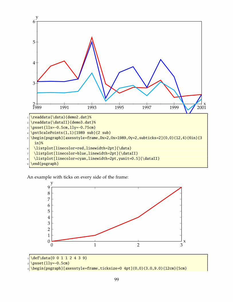
2

3

4

5

6

1989 1991 1993 1995 1997 1999 2001x

y



3 \psset{llx=0.5cm,lly=0.75cm}

4 \pstScalePoints(1,1){1989 sub}{2 sub}

5 \begin{psgraph}[axesstyle=frame,Dx=2,Ox=1989,Oy=2,subticks=2](0,0)(12,4){6in}{3

in}%


7 \listplot[linecolor=blue,linewidth=2pt]{\dataII}

8 \listplot[linecolor=cyan,linewidth=2pt,yunit=0.5]{\dataII}

9 \end{psgraph}

An example with ticks on every side of the frame:

0

1

2

3

4

5

6

7

8

9

0 1 2 3x

y

1 \def\data{0 0 1 1 2 4 3 9}

2 \psset{lly=0.5cm}

3 \begin{psgraph}[axesstyle=frame,ticksize=0 4pt](0,0)(3.0,9.0){12cm}{5cm}

99

4 \psaxes[axesstyle=frame,labels=none,ticksize=4pt 0](3,9)(0,0)(3,9)


6 \end{psgraph}

22.1 The new options

name default meaningxAxisLabel x label for the x-axisyAxisLabel y label for the y-axisxAxisLabelPos {} where to put the x-labelyAxisLabelPos {} where to put the y-labelllx 0pt trim for the lower left xlly 0pt trim for the lower left yurx 0pt trim for the upper right xury 0pt trim for the upper right y

There is one restriction in using the trim parameters, they must been set before psgraph

is called. They are senseless, when using as parameters of psgraph itself.

0

1

2

3

4

5

6

1989 1990 1991 1992 1993 1994 1995 1996 1997 1998 1999 2000 2001

Year

Wh

atev

er



3 \psset{llx=1cm,lly=1.25cm,urx=0.5cm,ury=0.1in,xAxisLabel=Year,%

4 yAxisLabel=Whatever,xAxisLabelPos={.4\linewidth,0.4in},%

5 yAxisLabelPos={0.4in,2in}}

6 \pstScalePoints(1,1){1989 sub}{}

7 \psframebox[linestyle=dashed,boxsep=0pt]{%

100

8 \begin{psgraph}[axesstyle=frame,Ox=1989,subticks=2](0,0)(12,6){0.8\linewidth

}{2.5in}%

9 \listplot[linecolor=red,linewidth=2pt]{\data}%

10 \listplot[linecolor=blue,linewidth=2pt]{\dataII}%

11 \listplot[linecolor=cyan,linewidth=2pt,yunit=0.5]{\dataII}%

12 \end{psgraph}%

13 }

22.2 Problems

Floating point operations in TEX are a real mess, which causes a lot of problems whenthere are very small oder very big units. With the options of \pstplot it is possible tochoose normal units (whatever this may be ...), but plotting the data as usual.

0

10

20

30

40

50

60

70

3.23 3.24 3.25 3.26x

y

�

�

�

1 \begin{filecontents*}{test.dat}

2 3.2345 34.5

3 3.2364 65.4

4 3.2438 50.2


6

7 \psset{lly=0.5cm,llx=1cm}

8 \readdata{\data}{test.dat}

9 \pstScalePoints(1,1){3.23 sub 100 mul}{}

10 \begin{psgraph}[Ox=3.23,Dx=0.01,dx=\psxunit,Dy=10](0,0)(3,70){0.8\linewidth}{5cm

}%

11 \listplot[showpoints=true,plotstyle=curve]{\data}

12 \end{psgraph}

This example shows some important facts:

• 3.23 sub 100 mul: the x values are now 0.45; 0.64; 1.38

• Ox=3.23: the origin of the x axis is set to 3.23

101

• Dx=0.01: the increment of the labels

• dx=\psxunit: uses the calculated unit value to get every unit a label

• Dy=10: increase the y labels by 10

Using the internal \psxunit one can have dynamical x-units, depending to the linewidthod the document.

23 \psStep

\psStep caclulates a step function for the upper or lower sum or the max/min of theRiemann integral definition of a given function. The available option is

StepType=lower|upper|Riemann

with lower as the default setting. The syntax of the function is

\psStep[options](x1,x2){n}{function}

(x1,x2) is the given Intervall for the step wise caculated function, n is the number ofthe rectangles and function is the mathematical function in postfix or algebraic notation(with algebraic=true).

0

1

2

0 1 2 3 4 5 6 7 8 9

0

1

2

−1

−2

1 2 3 4 5 6 7 8 9

102

0

1

−1

1 2 3 4 5 6 7 8 9

0

1

2

−1

−2

1 2 3 4 5 6 7 8 9

f(x) = 2 · √x · cos (lnx) · sinx

1 \begin{pspicture}(0.5,0.5)(10,3) \psaxes{>}(10,3)

2 \psplot[plotpoints=100,linewidth=1.5pt,algebraic,%

3 labelFontSize=\footnotesize]{0}{10}{sqrt(x)}

4 \psStep[linecolor=magenta,StepType=upper,fillstyle=hlines](0,9){9}{x sqrt}

5 \psStep[linecolor=blue,fillstyle=vlines](0,9){9}{x sqrt }

6 \end{pspicture}

7

8 \psset{plotpoints=200}

9 \begin{pspicture}(0.5,2.25)(10,3) \psaxes{>}(0,0)(0,2.25)(10,3)

10 \psplot[linewidth=1.5pt,algebraic,labelFontSize=\footnotesize]{0}{10}{sqrt(x)*sin(x)}

11 \psStep[algebraic,linecolor=magenta,StepType=upper](0,9){20}{sqrt(x)*sin(x)}

12 \psStep[linecolor=blue,linestyle=dashed](0,9){20}{x sqrt x RadtoDeg sin mul}

13 \end{pspicture}

14

15 \psset{yunit=1.25cm}

16 \begin{pspicture}(0.5,1.5)(10,1.5) \psaxes{>}(0,0)(0,1.5)(10,1.5)

17 \psStep[algebraic,StepType=Riemann,fillstyle=solid,fillcolor=black!10](0,10)

{50}%

18 {sqrt(x)*cos(x)*sin(x)}

19 \psplot[linewidth=1.5pt,algebraic,labelFontSize=\footnotesize]%

103

20 {0}{10}{sqrt(x)*cos(x)*sin(x)}

21 \end{pspicture}

22

23 \psset{unit=1.5cm}

24 \begin{pspicture}[plotpoints=200](0.5,3)(10,2.5)

25 \psStep[algebraic,fillstyle=solid,fillcolor=yellow](0.001,9.5){40}{2*sqrt(x)*cos(ln(x))*sin(x)}

26 \psStep[algebraic,StepType=Riemann,fillstyle=solid,fillcolor=blue](0.001,9.5)

{40}{2*sqrt(x)*cos(ln(x))*sin(x)}

27 \psaxes{>}(0,0)(0,2.75)(10,2.5)

28 \psplot[algebraic,linecolor=white,labelFontSize=\footnotesize]%

29 {0.001}{9.75}{2*sqrt(x)*cos(ln(x))*sin(x)}

30 \uput[90](6,1.2){$f(x)=2\cdot\sqrt{x}\cdot\cos{(\ln{x})}\cdot\sin{x}$}

31 \end{pspicture}

24 \psplotTangent

There is an additional option, named Derive vor an alternative function (see followingexample) to calculate the slope of the tangent. This will be in general the first derivation,but can also be any other function. If this option is different to to the default valueDerive=default, then this function is taken to calculate the slope. For the other cases,pstricksadd builds a secant with -0.00005<x<0.00005, calculates the slope and takes thisfor the tangent. This maybe problematic in some cases of special functions or x values,then it may be appropriate to use the Derivate option.

The macro expects three parameters:

x : the x value of the function for which the tangent should be calculated

dx : the dx to both sides of the x value

f(x) : the function in infix (with option algebraic) or the default postfix (PostScript)notation

The following examples show the use of the algebraic option together with the Deriveoption. Remember that using the algebraic option implies that the angles have to be inthe radian unit!

104

1

2

3

−1

−2

1 2 3 4 5 6 7−1−2−3−4−5−6−7

1 \def\F{x RadtoDeg dup dup cos exch 2 mul cos add exch 3 mul cos add}

2 \def\Fp{x RadtoDeg dup dup sin exch 2 mul sin 2 mul add exch 3 mul sin 3 mul add

neg}


4 \begin{pspicture}(7.5,2.5)(7.5,4)%X\psgrid

5 \psaxes{>}(0,0)(7.5,2)(7.5,3.5)

6 \psplot[linewidth=3\pslinewidth]{7}{7}{\F}

7 \psset{linecolor=red, arrows=<>, arrowscale=2}

8 \multido{\n=7+1}{8}{\psplotTangent{\n}{1}{\F}}

9 \psset{linecolor=magenta, arrows=<>, arrowscale=2}%

10 \multido{\n=0+1}{8}{\psplotTangent[linecolor=blue, Derive=\Fp]{\n}{1}{\F}}

11 \end{pspicture}

1

2

3

−1

−2

1 2 3 4 5 6 7−1−2−3−4−5−6−7

1 \def\Falg{cos(x)+cos(2*x)+cos(3*x)} \def\Fpalg{sin(x)2*sin(2*x)3*sin(3*x)}

2 \begin{pspicture}(7.5,2.5)(7.5,4)%\psgrid

3 \psaxes{>}(0,0)(7.5,2)(7.5,3.5)

4 \psplot[linewidth=1.5pt,algebraic,plotpoints=500]{7.5}{7.5}{\Falg}

105

5 \multido{\n=7+1}{8}{\psplotTangent[linecolor=red,arrows=<>,arrowscale=2,

algebraic]{\n}{1}{\Falg}}

6 \multido{\n=0+1}{8}{\psplotTangent[linecolor=magenta,%

7 arrows=<>,arrowscale=2,algebraic,Derive={\Fpalg}]{\n}{1}{\Falg}}

8 \end{pspicture}

The next example shows the use of Derive option to draw the perpendicular line of thetangent.

0

1

2

3

4

5

6

0 1 2 3 4 5 6

1 \begin{pspicture}(0.5,0.5)(7.25,7.25)

2 \def\Func{10 x div}

3 \psaxes[arrowscale=1.5]{>}(7,7)

4 \psplot[linewidth=2pt,algebraic]{1.5}{5}{10/x}

5 \psplotTangent[linewidth=.5\pslinewidth,

linecolor=red,algebraic]{3}{2}{10/x}

6 \psplotTangent[linewidth=.5\pslinewidth,

linecolor=blue,algebraic,Derive=(x*x)

/10]{3}{2}{10/x}

7 \psline[linestyle=dashed](!0 /x 3 def \Func)(!3

/x 3 def \Func)(3,0)

8 \end{pspicture}

24.1 A polarplot example

Let’s work with the classical cardioid : ρ = 2(1 + cos(θ)) anddρ

dθ= −2 sin(θ). The Derive

option always expects thedρ

dθvalue and uses internally the equation for the derivation of

implicit defined functions:

dy

dx=

ρ′ · sin θ + x

ρ′ · cos θ − y

where x = r · cos θ and y = r · sin θ

106

1

2

−1

−2

−3

1 2 3 4−1

1 \begin{pspicture}(1,3)(5,3)%\psgrid[subgridcolor=

lightgray]

2 \psaxes{>}(0,0)(1,3)(5,3)

3 \psplot[polarplot,linewidth=3\pslinewidth,linecolor=blue

,%

4 plotpoints=500]{0}{360}{1 x cos add 2 mul}

5 \end{pspicture}

1

2

−1

−2

−3

1 2 3 4−1


lightgray]

2 \psaxes{>}(0,0)(1,3)(5,3)

3 \psplot[polarplot,linewidth=3\pslinewidth,linecolor=blue,

plotpoints=500]{0}{360}{1 x cos add 2 mul}

4 \multido{\n=0+36}{10}{%

5 \psplotTangent[polarplot,linecolor=red,arrows=<>]{\n

}{1.5}{1 x cos add 2 mul} }

6 \end{pspicture}

1

2

−1

−2

−3

1 2 3 4−1


lightgray]

2 \psaxes{>}(0,0)(1,3)(5,3)

3 \psplot[polarplot,linewidth=3\pslinewidth,linecolor=blue,

algebraic,plotpoints=500]{0}{6.289}{2*(1+cos(x))}

4 \multido{\r=0.000+0.314}{21}{%

5 \psplotTangent[polarplot,Derive=2*sin(x),algebraic,

linecolor=red,arrows=<>]{\r}{1.5}{2*(1+cos(x))} }

6 \end{pspicture}

24.2 A \parametricplot example

Let’s work with a Lissajou curve :

{

x = 3.5 cos(2t)y = 3.5 sin(6t)

whose derivative is :

{

x = −7 sin(2t)y = 21 cos(6t)

The parameter must be the letter t instead of x and when using the algebraic optiondivide the two equations by a | (see example).

107

1 \def\Lissa{t dup 2 RadtoDeg mul cos 3.5 mul exch 6 mul RadtoDeg sin 3.5 mul}%

2 \psset{yunit=0.6}


4 \parametricplot[plotpoints=500,linewidth=3\pslinewidth]{0}{3.141592}{\Lissa}

5 \multido{\r=0.000+0.314}{11}{%

6 \psplotTangent[linecolor=red,arrows=<>]{\r}{1.5}{\Lissa} }

7 \multido{\r=0.157+0.314}{11}{%

8 \psplotTangent[linecolor=blue,arrows=<>]{\r}{1.5}{\Lissa} }

9 \end{pspicture}\hfill%

10 \def\LissaAlg{3.5*cos(2*t)|3.5*sin(6*t)} \def\LissaAlgDer{7*sin(2*t)|21*cos(6*t)}%


12 \parametricplot[algebraic,plotpoints=500,linewidth=3\pslinewidth]{0}{3.141592}{\LissaAlg

}

13 \multido{\r=0.000+0.314}{11}{%

14 \psplotTangent[algebraic,linecolor=red,arrows=<>]{\r}{1.5}{\LissaAlg} }

15 \multido{\r=0.157+0.314}{11}{%

16 \psplotTangent[algebraic,linecolor=blue,arrows=<>,%

17 Derive=\LissaAlgDer]{\r}{1.5}{\LissaAlg} }

18 \end{pspicture}

25 Successive derivatives of a function

The new PostScript function Derive has been added for plotting the succesive derivativesof a function. It must be used wiht the algebaic option. This function has two arguments:

1. a positive integer with define the order of the derivative, obviously 0 means thefunction itself!

2. a function of variable x which can be any function using the common operators,

Do not think that the derivative is approximated, the internal PostScript engine willcompute the real derivative using a formal derivative engine.

108

The following diagram contains the plot of the polynomial:

f(x) =14∑

i=0

(−1)ix2i

i!= 1 − x2

2+x4

4!− x6

6!+x8

8!− x10

10!+x12

12!− x14

14!

and of its 15 first derivatives. It is the sequence definition of the cosine.

0 1 2 3 4 5 6 7-1

0

1

1 \psset{unit=2}

2 \def\getColor#1{\ifcase#1 Tan\or RedOrange\or magenta\or yellow\or green\or Orange\or blue

\or

3 DarkOrchid\or BrickRed\or Rhodamine\or OliveGreen\or Goldenrod\or Mahogany\or

4 OrangeRed\or CarnationPink\or RoyalPurple\or Lavender\fi}

5 \begin{pspicture}[showgrid=true](0,1.2)(7,1.5)

6 \psclip{\psframe[linestyle=none](0,1.1)(7,1.1)}

7 \multido{\in=0+1}{16}{%

8 \psplot[linewidth=1pt,algebraic=true,linecolor=\getColor{\in},linewidth=1pt]{0}{7}

9 {Derive(\in,1x^2/2+x^4/24x^6/720+x^8/40320x^10/3628800+x^12/479001600x

^14/87178291200)}}

10 \endpsclip

11 \end{pspicture}

0 1 2 3-2

-1

0

1

2

3

1 \begin{pspicture}[shift=2.5,showgrid=true,linewidth=1pt

](0,2)(3,3)

2 \psplot[algebraic=true]{.001}{3}{x*ln(x)} % f(x)

3 \psplot[algebraic=true,linecolor=red]{.05}{3}{Derive(1,x*ln(

x))} % f’(x)=1+ln(x)

4 \end{pspicture}

109

26 Variable step for plotting a curve

26.1 Theory

As you know with the \psplot macro, the curve is plotted using a piece wise linear curve.The step is given by the parameter plotpoints. For each step between xi and xi+1, thearea defined between the curve and its approximation (a segment) is majored by thisformula :

|ε| ≤ M2(f)(xi+1 − xi)3

12

M2(f) is a majorant of the second derivativeof f in the interval [xi;xi+1].

0 1 2 3 4 5 6-1

0

1

2

3

xn xn+1

ε

The parameter VarStep (false by default) activates the variable step algorithm. It isset to a tolerance defines by the parameter VarStepEpsilon (default by default, acceptreal value). If this parameter is not set by the user, then it is automatically computedusing the default first step given by the parameter plotpoints. Then, for each step,f ′′(xn) and f ′′(xn+1) are computed and the smaller is used as M2(f), and then the step isapproximated. This means that the step is constant for a second order polynomials.

26.2 The cosine

Different value for the tolerance from 0.01 to 0.000 1, a factor 10 between each of them.In black, there is the classical psplot behavior, and in magenta the default variable stepbehavior.

0 1 2 3-1

0

1

2

�

�

�

�

�

�

��

� ��

�

�

�

�

�

�

�

�

��

� � � ��

�

�

�

�

�

�

�

�

�

�

�

��

��

�

�

�

�

�

�

�

��

��

110

1 \psset{algebraic=true, VarStep=true, unit=2, showpoints=true, linecolor=red}

2 \begin{pspicture}[showgrid=true](0,1)(3.14,2)

3 \psplot[VarStepEpsilon=.01]{0}{3.14}{cos(x)}

4 \psplot[VarStepEpsilon=.001]{0}{3.14}{cos(x)+.15}

5 \psplot[VarStepEpsilon=.0001]{0}{3.14}{cos(x)+.3}

6 \psplot[linecolor=magenta]{0}{3.14}{cos(x)+.45}

7 \psplot[VarStep=false,linewidth=1pt,linecolor=black]{0}{3.14}{cos(x)+.6}

8 \end{pspicture}

26.3 The neperian Logarithm

A really classical example wich gives a bad beginning, the tolerance is set to 0.001.

0 1 2 3 4 5 6 7 8 9 10 11 12 13 14 15 16-5

-4

-3

-2

-1

0

1

2

3

4

�

�

�

�

�

�

��

��

��

��

��

� � � � � � � � � � � � � � � � � � � � � � � � � � � � � � � � � �

�

�

�

�

�

�

�

�

�

�

�

�

�

�

�

�

�

�

�

�

�

��

��

��

��

��

��

��

��

�

�

�

�

�

�

�

�

�

�

�

�

�

�

�

�

�

1 \psset{algebraic=true, VarStep=true, linecolor=red, showpoints=true}


3 \psplot[VarStep=false, linecolor=black]{.01}{16}{ln(x)+1}

4 \psplot[linecolor=magenta]{.51}{16}{ln(x1/2)+1/2}

5 \psplot[VarStepEpsilon=.001]{1.01}{16}{ln(x1)}

6 \psplot[VarStepEpsilon=.01]{1.51}{16}{ln(x1.5)100/200}

7 \end{pspicture}

111

26.4 Sinus of the inverse of x

Impossible to draw, but let’s try!

0-1

0

1

�

�

�

�

�

�

�

�

�

�

�

�

�

�

��

�

�

�

�

�

�

�

�

�

��

��

�

�

�

�

�

��

�

�

�

�

�

�

�

�

�

�

�

�

�

�

�

�

�

��

�

�

�

��

�

�

�

� �

�

�

�

�

� ��

�

�

�

�

��

� �

0-1

0

1

�

�

�

�

�

�

�

�

�

�

�

�

�

�

�

�

�

�

�

�

�

�

��

�

�

�

�

�

��

�

�

�

�

�

��

�

�

��

�

�

��

�

�

��

�

�

��

�

�

�

�

�

�

�

��

�

�

�

�

�

�

��

�

�

�

��

�

�

�

��

�

�

�

��

�

�

�

��

�

�

�

�

��

�

�

�

�

��

�

�

�

�

��

�

�

�

�

�

��

�

�

�

�

�

��

��

�

�

�

�

��

��

�

�

�

��

��

��

� �

0-1

0

1

�

��

�

�

�

��

�

�

�

�

��

�

�

�

�

��

�

�

�

�

��

�

�

�

�

��

�

�

�

�

��

�

�

�

�

��

�

�

�

�

��

�

�

�

�

��

�

�

�

�

��

�

�

�

�

��

�

�

�

�

��

�

�

�

�

��

�

�

�

�

��

�

�

�

�

��

�

�

�

�

��

�

�

�

�

��

�

�

�

�

��

�

�

�

�

��

�

�

�

�

�

��

�

�

�

�

��

�

�

�

�

��

�

�

�

�

��

�

�

�

�

��

�

�

�

�

��

�

�

�

��

�

�

��

��

�

��

��

��

��

0-1

0

1

�

�

��

�

�

�

�

�

�

�

�

��

�

�

� �

�

�

�

�

��

��

�

�

�

�

��

��

��

1 \psset{xunit=64,algebraic,VarStep,linecolor=red,showpoints=true,linewidth=1pt}

2 \begin{pspicture}[showgrid=true](0,1)(.5,1)

3 \psplot[VarStepEpsilon=.0001]{.01}{.25}{sin(1/x)}

4 \end{pspicture}\\



7 \end{pspicture}\\



10 \end{pspicture}\\


12 \psplot[VarStep=false, linecolor=black]{.01}{.25}{sin(1/x)}

13 \end{pspicture}

26.5 A really complex function

Just appreciate the difference between the normal behavior and the plotting with thevarStep option. The function is :

f(x) = x − x2

10+ ln(x) + cos(2x) + sin(x2) − 1

112

0 1 2 3 4 5-2

-1

0

1

2

3

4

5

6

�

�

�

�

�

�

�

�

�

�

��

� � ��

�

��

��

�

�

�

�

�

�

�

�

��

�

�

�

�

�

��

�

�

�

�

��

�

�

�

�

�

�

��

�

�

�

�

��

�

�

�

�

��

�

�

��

�

�

�

�

�

� �

�

� �

�

�

�

�

�

�

�

�

�

�

�

�

�

��

�

��

�

�

�

�

�

�

�

�

�

�

�

��

��

��

��

��

�

�

�

�

�

�

�

� �

�

�

�

��

�

�

��

�

�

�

�

�

�

�

�

�

� �

�

1 \psset{xunit=3, algebraic, VarStep, showpoints=true}


3 \psplot[VarStepEpsilon=.0005, linecolor=red]{.1}{5}{xx^2/10+ln(x)+cos(2*x)+

sin(x^2)}

4 \psplot[linecolor=magenta]{.1}{5}{xx^2/10+ln(x)+cos(2*x)+sin(x^2)+.5}

5 \psplot[VarStep=false]{.1}{5}{xx^2/10+ln(x)+cos(2*x)+sin(x^2)1}

6 \end{pspicture}

26.6 A hyperbola

��

�

�

�

�

�

�

�

�

�

�

�

�

�

��

1

2

3

4

5

−1

−2

−3

−4

1 2 3 4 5 6 7 8−1−2−3−4−5

113

1 \psset{algebraic=true, showpoints=true, unit=0.75}


3 \psplot[linecolor=black]{5}{1.8}{(x1)/(x2)}

4 \psplot[VarStep=true, VarStepEpsilon=.001, linecolor=red]{2.2}{9}{(x1)/(x2)}

5 \psaxes{>}(0,0)(5,4)(9,6)

6 \end{pspicture}

26.7 Successive derivatives of a polynom

0 1 2 3 4 5 6 7-1

0

1�

�

�

�

�

�

�

�

�

�

��

�

�

�

�

�

�

�

�

�

��

�

�

�

�

�

��

�

�

�

�

��

�

�

�

�

�

�

�

�

�

��

�

�

�

�

�

�

�

�

��

�

�

�

�

�

�

�

�

��

�

�

�

�

�

�

�

�

�

�

�

�

�

��

�

�

�

�

�

�

�

�

�

��

�

��

�

�

�

�

�

�

�

�

��

�

�

�

�

�

�

��

�

�

�

�

�

�

�

�

��

�

�

�

�

�

�

�

�

� � �

�

�

�

�

�

�

��

�

�

�

�

�

�

�

�

��

�

�

�

�

�

�

�

�

�

�

�

�

��

�

�

�

�

�

�

�

�

��

�

�

�

�

�

�

�

�

�

�

�

�

�

��

�

�

�

��

�

�

�

��

�

�

�

�

�

�

�

��

�

�

�

�

�

�

�

�

�

�

��

�

�

�

�

�

�

�

�

��

�

�

�

�

�

�

�

�

�

�

�

� � � � � � �

� � � � � � �

1 \psset{unit=2, algebraic=true, VarStep=true, showpoints=true, VarStepEpsilon

=.001}

2 \def\getColor#1{\ifcase#1 Tan\or RedOrange\or magenta\or yellow\or green\or

Orange\or blue\or

3 DarkOrchid\or BrickRed\or Rhodamine\or OliveGreen\or Goldenrod\or Mahogany\or

4 OrangeRed\or CarnationPink\or RoyalPurple\or Lavender\fi}

5 \begin{pspicture}[showgrid=true](0,1.2)(7,1.5)

6 \psclip{\psframe[linestyle=none](0,1.1)(7,1.1)}

7 \multido{\in=0+1}{16}{%

8 \psplot[algebraic=true, linecolor=\getColor{\in}]{0.1}{7}

9 {Derive(\in,Sum(i,0,1,7,(1)^i*x^(2*i)/Fact(2*i)))}}

10 \endpsclip

11 \end{pspicture}

114

26.8 The variable step algorithm together with the IfTE primitive

-7 -6 -5 -4 -3 -2 -1 0 1 2-2

-1

0

1

2

3

4�

�

�

�

�

�

�

�

�

�

��

�

�

�

�

�

�

�

�

�

�

�

��

�

�

�

�

�

� � � � � ��

�

�

�

�

�

�

�

�

�

�

�

�

�

�

�

�

�

�

�

�

�

�

�

�

�

�

�

�

��

��

�

�

�

�

�

�

�

1 \psset{unit=1.5, algebraic, VarStep, showpoints=true, VarStepEpsilon=.001}


3 \psplot{7}{2}{IfTE(x<5,(x+5)^3/2,IfTE(x<0,0,x^2))}

4 \psplot{7}{2}{5*x/9+26/9}

5 \psplot[linecolor=blue]{7}{2}{(x+7)^30/9^30*4.51/2}

6 \psplot[linecolor=red]{6.9}{2}

7 {IfTE(x<6,ln(x+7),IfTE(x<3,x+6,IfTE(x<0.1415926,sin(x+3)+3,3.1415926x))

)}

8 \end{pspicture}

26.9 Using \parametricplot

-1 0 1-1

0

1

�

�

�

�

�

�

�

�

�

��

��

��

�

�

�

�

�

�

�

�

�

�

�

�

�

�

��

��

�

�

�

�

�

�

�

�

�

�

�

�

�

�

�

�

�

�

��

��

�

�

�

�

�

�

�

�

�

�

�

�

�

�

��

��

�

�

�

�

�

�

�

�

��

-1 0 1-1

0

1

115

1 \psset{unit=3}


3 \parametricplot[algebraic=true,linecolor=red,VarStep=true, showpoints=true,

4 VarStepEpsilon=.0001]

5 {3.14}{3.14}{cos(3*t)|sin(2*t)}

6 \end{pspicture}


8 \parametricplot[algebraic=true,linecolor=blue,VarStep=true, showpoints=false,


10 {3.14}{3.14}{cos(3*t)|sin(2*t)}

11 \end{pspicture}

-1 0 1-1

0

1

�

�

�

�

�

�

�

�

�

��

��

�

�

�

�

�

�

�

�

�

�

�

�

�

�

�

��

��

��

��

�

�

�

�

�

�

�

�

�

�

�

�

�

�

�

��

��

�

�

�

�

�

�

�

�

�

�

�

�

�

�

�

�

�

�

��

� � ��

�

�

�

�

�

�

�

�

�

�

�

�

�

�

�

�

��

��

��

��

�

�

�

�

�

�

�

�

�

�

�

�

�

�

��

��

��

�

�

�

�

�

�

�

�

�

�

�

�

�

�

�

�

��

��

��

�

�

�

�

�

�

�

�

�

�

�

�

�

�

�

��

��

��

��

�

�

�

�

�

�

�

�

�

�

�

�

�

�

��

��

�

�

�

�

�

�

�

�

�

�

�

�

�

�

�

�

��

��

��

�

�

�

�

�

�

�

�

�

�

�

�

�

�

�

�

��

��

��

��

�

�

�

�

�

�

�

�

�

�

�

�

�

�

��

��

�

�

�

�

�

�

�

�

�

�

�

�

�

�

�

�

��

��

��

�

�

�

�

�

�

�

�

�

�

�

�

�

�

�

��

��

��

��

�

�

�

�

�

�

�

�

�

�

�

�

�

�

��

��

�

�

�

�

�

�

�

�

�

�

�

�

�

�

�

�

��

��

��

�

�

�

�

�

�

�

�

�

�

�

�

�

�

�

�

��

��

��

�

�

�

�

�

�

�

�

�

�

�

�

�

�

�

�

��

��

�

�

�

�

�

�

�

�

�

�

�

�

�

�

�

�

��

��

��

�

�

�

�

�

�

�

�

�

�

�

�

�

�

�

��

��

��

�

�

�

�

�

�

�

�

�

�

�

�

�

�

�

�

��

��

�

�

�

�

�

�

�

�

�

�

�

�

�

�

�

�

��

��

��

�

�

�

�

�

�

�

�

�

�

�

�

�

�

�

�

��

��

��

�

�

�

�

�

�

�

�

�

�

�

�

�

�

�

�

��

��

�

�

�

�

�

�

�

�

�

�

�

�

�

�

�

�

��

��

�

�

�

�

�

�

�

�

�

�

�

�

�

�

�

��

��

��

�

�

�

�

�

�

�

�

�

�

�

�

�

�

�

�

��

��

�

�

�

�

�

�

�

�

�

�

�

�

�

�

�

�

��

� � � ��

�

�

�

�

�

�

�

�

�

�

�

�

�

�

�

�

��

��

��

�

�

�

�

�

�

�

�

�

�

�

�

�

�

�

�

��

��

�

�

�

�

�

�

�

�

�

�

�

�

�

�

�

�

��

��

�

�

�

�

�

�

�

�

�

�

�

�

�

�

�

��

��

��

�

�

�

�

�

�

�

�

�

�

�

�

�

�

�

�

��

��

�

�

�

�

�

�

�

�

�

�

�

�

�

�

�

�

��

� � � ��

�

�

�

�

�

�

�

�

�

�

�

�

�

�

�

�

��

��

��

�

�

�

�

�

�

�

�

�

�

�

�

�

�

�

�

��

��

�

�

�

�

�

�

�

�

�

�

�

�

�

�

�

�

��

��

�

�

�

�

�

�

�

�

�

�

�

�

�

�

�

��

��

��

�

�

�

�

�

�

�

�

�

�

�

�

�

�

�

�

��

��

�

�

�

�

�

�

�

�

�

�

�

�

�

�

�

�

��

� � � ��

�

�

�

�

�

�

�

�

�

�

�

�

�

�

�

�

��

��

��

�

�

�

�

�

�

�

�

�

�

�

�

�

�

�

�

��

��

�

�

�

�

�

�

�

�

�

�

�

�

�

�

�

�

��

��

�

�

�

�

�

�

�

�

�

�

�

�

�

�

�

��

��

��

�

�

�

�

�

�

�

�

�

�

�

�

�

�

�

�

��

��

�

�

�

�

�

�

�

��

-1 0 1-1

0

1

1 \psset{unit=2.5}


3 \parametricplot[algebraic=true,linecolor=red,VarStep=true, showpoints=true,


5 {0}{47.115}{cos(5*t)|sin(3*t)}

6 \end{pspicture}


8 \parametricplot[algebraic=true,linecolor=blue,VarStep=true, showpoints=false,


10 {0}{47.115}{cos(5*t)|sin(3*t)}

11 \end{pspicture}

0 1 2 3 4 5 6 7 8 9 10 11 12 130

1

2

��

�

�

�

�

� �

�

�

�

�

��

�

�

�

�

��

�

�

�

�

�

��

0 1 2 3 4 5 6 7 8 9 10 11 12 130

1

2

1 \psset{xunit=.5}


3 \parametricplot[algebraic,linecolor=red,VarStep, showpoints=true,

116

4 VarStepEpsilon=.01]{0}{12.566}{t+cos(tPI/2)|1+sin(tPI/2)}

5 \end{pspicture}

6 %


8 \parametricplot[algebraic,linecolor=blue,VarStep, showpoints=false,

9 VarStepEpsilon=.001]{0}{12.566}{t+cos(tPI/2)|1+sin(tPI/2)}

10 \end{pspicture}

27 New math functions and their derivative

27.1 The inverse sin and its derivative

-1 0 1-2

-1

0

1

2

-1 0 1-2

-1

0

1

2

��

�

�

�

�

�

�

�

�

�

�

�

��

-1 0 10

1

2

3

4 �

�

�

�

�

�

�

�

��

� � ��

�

�

�

�

�

�

�

�

�

-1 0 10

1

2

3

4 �

�

�

�

�

�

�

�

�

�

�

��

��

�

�

�

�

�

�

�

�

�

�

�

�

1 \psset{unit=1.5}


3 \psplot[linecolor=blue,algebraic]{1}{1}{asin(x)}

4 \end{pspicture}

5 \hspace{1em}

6 \psset{algebraic, VarStep, VarStepEpsilon=.001, showpoints=true}


8 \psplot[linecolor=blue]{.999}{.999}{asin(x)}

9 \end{pspicture}

10 \hspace{1em}


12 \psplot[linecolor=red]{.97}{.97}{Derive(1,asin(x))}

13 \end{pspicture}

14 \hspace{1em}



17 \psplot[linecolor=red]{.97}{.97}{Derive(1,asin(x))}

18 \end{pspicture}

117

27.2 The inverse cosine and its derivative

-1 0 10

1

2

3

-1 0 10

1

2

3 ��

�

�

�

�

�

�

�

�

�

�

�

��

-1 0 1-4

-3

-2

-1

�

�

�

�

�

�

�

�

��

� � ��

�

�

�

�

�

�

�

�

� -1 0 1-4

-3

-2

-1

�

�

�

�

�

�

�

�

�

�

�

��

��

�

�

�

�

�

�

�

�

�

�

�

�

1 \psset{unit=1.5}


3 \psplot[linecolor=blue,algebraic]{1}{1}{acos(x)}

4 \end{pspicture}

5 \hspace{1em}



8 \psplot[linecolor=blue]{.999}{.999}{acos(x)}

9 \end{pspicture}

10 \hspace{1em}


12 \psplot[linecolor=red]{.97}{.97}{Derive(1,acos(x))}

13 \end{pspicture}

14 \hspace{1em}



17 \psplot[linecolor=red]{.97}{.97}{Derive(1,acos(x))}

18 \end{pspicture}

118

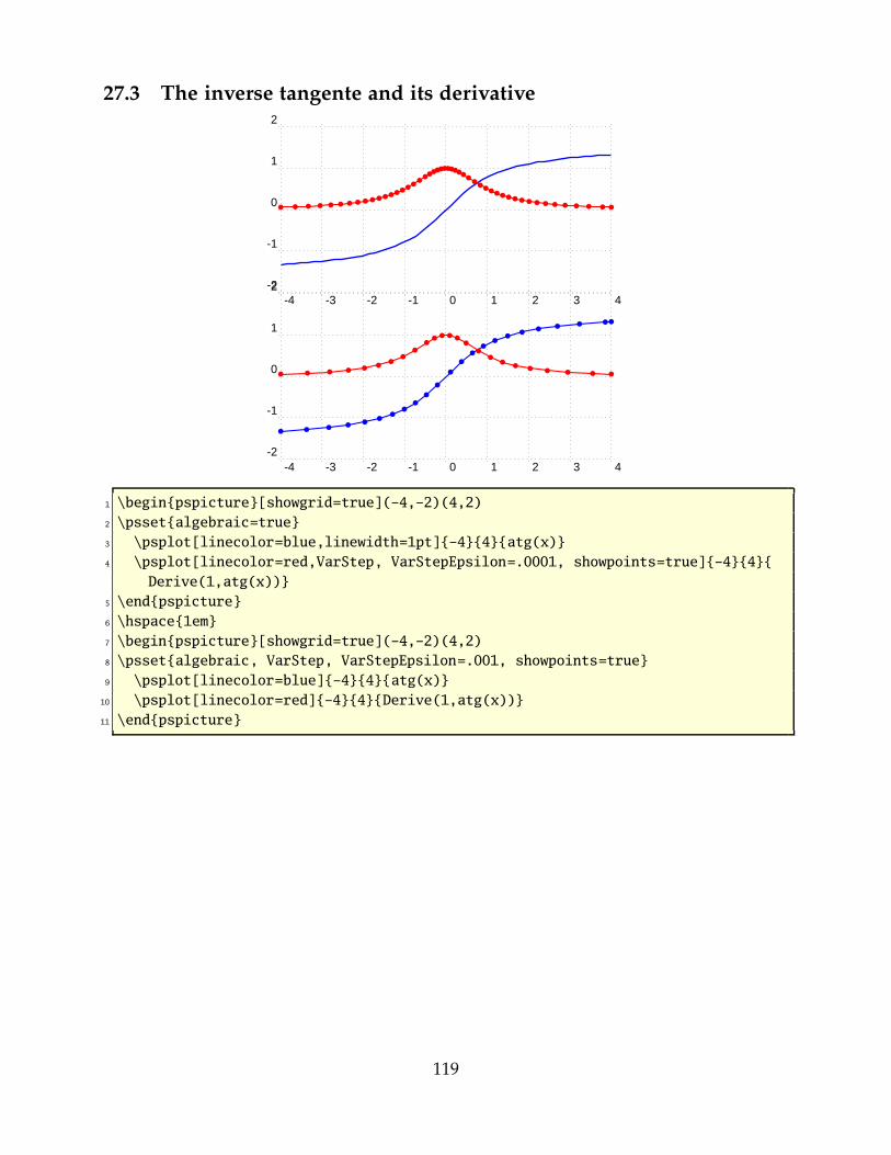
27.3 The inverse tangente and its derivative

-4 -3 -2 -1 0 1 2 3 4-2

-1

0

1

2

� � � � � � � � � ��

��

��

-4 -3 -2 -1 0 1 2 3 4-2

-1

0

1

2

� � � ��

��

��

�

�

�

�

�

��

��

��

� � � � ��

��

�

��

� ��

��

��

� � � � �


2 \psset{algebraic=true}

3 \psplot[linecolor=blue,linewidth=1pt]{4}{4}{atg(x)}

4 \psplot[linecolor=red,VarStep, VarStepEpsilon=.0001, showpoints=true]{4}{4}{

Derive(1,atg(x))}

5 \end{pspicture}

6 \hspace{1em}



9 \psplot[linecolor=blue]{4}{4}{atg(x)}

10 \psplot[linecolor=red]{4}{4}{Derive(1,atg(x))}

11 \end{pspicture}

119

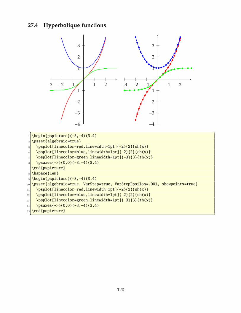
27.4 Hyperbolique functions

1

2

3

−1

−2

−3

−4

1 2−1−2−3

�

�

�

�

�

�

�

�

�

�

�

�

�

�

�

�

�

�

�

��

�

�

�

�

�

�

�

��

��

�

�

�

�

�

�

�

�

� � � � ��

�

�

�

�

��

� � � � �1

2

3

−1

−2

−3

−4

1 2−1−2−3



3 \psplot[linecolor=red,linewidth=1pt]{2}{2}{sh(x)}

4 \psplot[linecolor=blue,linewidth=1pt]{2}{2}{ch(x)}

5 \psplot[linecolor=green,linewidth=1pt]{3}{3}{th(x)}

6 \psaxes{>}(0,0)(3,4)(3,4)

7 \end{pspicture}

8 \hspace{1em}


10 \psset{algebraic=true, VarStep=true, VarStepEpsilon=.001, showpoints=true}

11 \psplot[linecolor=red,linewidth=1pt]{2}{2}{sh(x)}

12 \psplot[linecolor=blue,linewidth=1pt]{2}{2}{ch(x)}

13 \psplot[linecolor=green,linewidth=1pt]{3}{3}{th(x)}

14 \psaxes{>}(0,0)(3,4)(3,4)

15 \end{pspicture}

120

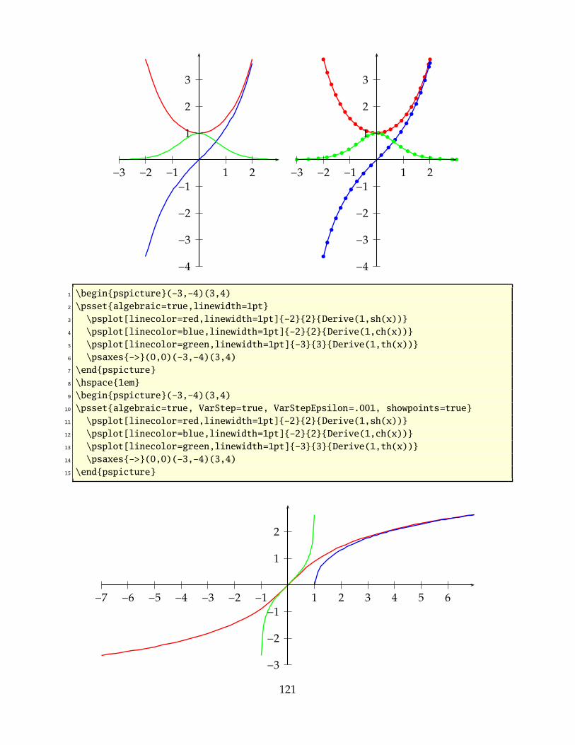
1

2

3

−1

−2

−3

−4

1 2−1−2−3

�

�

�

�

�

�

�

��

��

�

�

�

�

�

�

�

�

�

�

�

�

�

�

�

�

�

�

�

�

�

�

�

�

�

�

�

��

� � � � ��

�

��

��

��

1

2

3

−1

−2

−3

−4

1 2−1−2−3


2 \psset{algebraic=true,linewidth=1pt}

3 \psplot[linecolor=red,linewidth=1pt]{2}{2}{Derive(1,sh(x))}

4 \psplot[linecolor=blue,linewidth=1pt]{2}{2}{Derive(1,ch(x))}

5 \psplot[linecolor=green,linewidth=1pt]{3}{3}{Derive(1,th(x))}

6 \psaxes{>}(0,0)(3,4)(3,4)

7 \end{pspicture}

8 \hspace{1em}



11 \psplot[linecolor=red,linewidth=1pt]{2}{2}{Derive(1,sh(x))}

12 \psplot[linecolor=blue,linewidth=1pt]{2}{2}{Derive(1,ch(x))}

13 \psplot[linecolor=green,linewidth=1pt]{3}{3}{Derive(1,th(x))}

14 \psaxes{>}(0,0)(3,4)(3,4)

15 \end{pspicture}

1

2

−1

−2

−3

1 2 3 4 5 6−1−2−3−4−5−6−7

121

��

��

��

��

��

�

�

�

�

�

�

�

�

�

�

��

��

��

��

��

��

�

�

�

��

��

��

��

��

��

�

�

�

�

�

�

�

�

�

�

�

�

�

�

�

�

�

�

�

�

�

��

1

2

−1

−2

−3

1 2 3 4 5 6−1−2−3−4−5−6−7



3 \psplot[linecolor=red,linewidth=1pt]{7}{7}{Argsh(x)}

4 \psplot[linecolor=blue,linewidth=1pt]{1}{7}{Argch(x)}

5 \psplot[linecolor=green,linewidth=1pt]{.99}{.99}{Argth(x)}

6 \psaxes{>}(0,0)(7,3)(7,3)

7 \end{pspicture}\\[\baselineskip]



10 \psplot[linecolor=red,linewidth=1pt]{7}{7}{Argsh(x)}

11 \psplot[linecolor=blue,linewidth=1pt]{1.001}{7}{Argch(x)}

12 \psplot[linecolor=green,linewidth=1pt]{.99}{.99}{Argth(x)}

13 \psaxes{>}(0,0)(7,3)(7,3)

14 \end{pspicture}

1

2

3

4

5

0 1 2 3 4 5 6−1−2−3−4−5−6−7

122

� � � � � � � ��

��

��

��

� � � � � � � �

�

�

�

�

�

�

�

�

�

��

� � � � � � � �

�

�

�

�

�

�

�

�

��

��

�

�

�

�

�

�

�

�

�

1

2

3

4

5

0 1 2 3 4 5 6−1−2−3−4−5−6−7



3 \psplot[linecolor=red,linewidth=1pt]{7}{7}{Derive(1,Argsh(x))}

4 \psplot[linecolor=blue,linewidth=1pt]{1.014}{7}{Derive(1,Argch(x))}

5 \psplot[linecolor=green,linewidth=1pt]{.9}{.9}{Derive(1,Argth(x))}

6 \psaxes{>}(0,0)(7,0)(7,6)

7 \end{pspicture}\\[\baselineskip]




11 \psplot[linecolor=red,linewidth=1pt]{7}{7}{Derive(1,Argsh(x))}

12 \psplot[linecolor=blue,linewidth=1pt]{1.014}{7}{Derive(1,Argch(x))}

13 \psplot[linecolor=green,linewidth=1pt]{.9}{.9}{Derive(1,Argth(x))}

14 \psaxes{>}(0,0)(7,0)(7,6)

15 \end{pspicture}

123

28 \psplotDiffEqn – solving diffential equations

A differential euqation of first order is like

y′ = f(x, y, y′) (1)

where y is a function of x. We define some vectors Y = [y, y′, · · · , y(n−1)] und Y ′ =

[y′, y′′, · · · , yn], depending to the order n. The syntax of the macro is

\psplotDiffEqn[options]{x0}{x1}{y0}{f(x,y,y’,...)}

• options: the \psplotDiffEqn specific options and all other of PSTricks, which makesense;

• x0: the start value;• x1: the end value of the definition interval;• y0: the initial values for y(x0) y

′(x0) . . .;• f(x, y, y′, ...): the differential equation, depending to the number of initial values,

e.g.: {0 1} for y0 are two initial values, so that we have a differential equation ofsecond order f(x, y, y′) and the macro leaves y y′ on the stack.

The new options are:

• method: integration method (euler for order 1 euler method, rk4 for 4th orderRunge-Kutta method);

• whichabs: select the abscissa for plotting the graph, by default it is x, but you canspecify a number which represent a position in the vector y;

• whichord: same as precedent for the ordinate, by default y(0);• plotfuncx: describe a ps function for the abscissa, parameter whichabs becomes

useless;• plotfuncy: idem for ordoinate;• buildvector: boolean parameter for specifying the input-output of the f descrip-

tion:

true (default): y is put on the stack element by element, y′ must be given in thesame way;

false : y is put on the stack as a vector, y′ must be returned in the same way;

• algebraic: algebraic description for f , buildvector parameter is useless whenactivating this option.

124

28.1 Variable step for differential equations

A new algorithm has been added for adjusting the step according to the variations ofthe curve. The parameter method has a new possible value : varrkiv to activate theRunge-Kutta method with variable step, then the parameter varsteptol (real value; .01by default) can control the tolerance of the algortihm.

0 1 2 3 4 5 6 7 8 9 100

1�

�

�

��

�

�

�

�

�

�

��

�

�

�

�

�

�

�

��

� � � � � � � � � � � � � �

�

�

�

�

�

�

�

�

�

�

��

��

� � � � � � � � � � � � � � � � � � � � � � � � � �

RK ordre 4 : ε < 10−1

RK ordre 4 : ε < 10−2

RK ordre 4 : ε < 10−3

RK ordre 4 : ε < 10−4

solution exacte

Figure 1: Equation y′ = −y with y0 = 1.

1 \def\Funct{neg}\def\FunctAlg{y[0]}

2 \psset{xunit=1.5, yunit=8, showpoints=true}

3 \begin{pspicture}[showgrid=true](0,0)(10,1.2)

4 \psplot[linewidth=6\pslinewidth, linecolor=green, showpoints=false

]{0}{10}{2.71828182846 x neg exp}

5 \psplotDiffEqn[linecolor=magenta, method=varrkiv, varsteptol=.1, plotpoints

=2]{0}{10}{1}{\Funct}

6 \rput(0,.0){\psplotDiffEqn[linecolor=blue, method=varrkiv, varsteptol=.01,

plotpoints=2]{0}{10}{1}{\Funct}}

7 \rput(0,.1){\psplotDiffEqn[linecolor=Orange, method=varrkiv, varsteptol=.001,


8 \rput(0,.2){\psplotDiffEqn[linecolor=red, method=varrkiv, varsteptol=.0001,


9 \psset{linewidth=4\pslinewidth,showpoints=false}

10 \rput*(3.3,.9){\psline[linecolor=magenta](.75cm,0)}

11 \rput*[l](3.3,.9){\small RK ordre 4 : $\varepsilon<10^{1}$}

12 \rput*(3.3,.8){\psline[linecolor=blue](.75cm,0)}

125


14 \rput*(3.3,.7){\psline[linecolor=Orange](.75cm,0)}


16 \rput*(3.3,.6){\psline[linecolor=red](.75cm,0)}


18 \rput*(3.3,.5){\psline[linecolor=green](.75cm,0)}

19 \rput*[l](3.3,.5){\small solution exacte}

20 \end{pspicture}

0

1

−1

1 2 3 4 5 6 7 8 9

��

�

�

�

�

�

�

�

�

�

�

�

��

�

�

�

�

�

�

�

�

�

�

�

�

��

�

�

�

�

�

�

�

�

�

�

�

��

�

��

�

�

�

�

�

�

�

��

�

�

�

�

�

� �

�

�

�

�

� �

�

�

�

�

��

�

��

�

�

�

�

��

�

�

�

�

�

�

�

�

�

�

�

�

�

��

�

�

�

�

�

�

�

�

�

�

��

�

�

�

�

�

�

�

�

�

�

�

�

�

�

�

�

�

�

�

�

�

�

�

�

�

��

�

�

�

�

�

�

�

�

�

�

�

�

�

��

�

�

�

�

�

�

�

�

�

�

�

�

�

�

� �

�

�

�

�

�

�

�

�

�

�

�

�

�

�

� �

�

�

�

ε < 10−1

ε < 10−2

ε < 10−3

ε < 10−4

ε < 10−5

solution exacte

Figure 2: Equation y′′ = −y

1 \def\Funct{exch neg}

2 \psset{xunit=1.5, yunit=5, method=varrkiv, showpoints=true}%%

3 \def\quatrepi{12.5663706144}

4 \begin{pspicture}(0,1)(10,1.3)

5 \psaxes{>}(0,0)(0,1)(10,1.3)

6 \psplot[linewidth=4\pslinewidth, linecolor=green, algebraic=true]{0}{10}{cos(x

)}

7 \rput(0,.0){\psplotDiffEqn[linecolor=magenta, plotpoints=7, varsteptol

=.1]{0}{10}{1 0}{\Funct}}

8 \rput(0,.0){\psplotDiffEqn[linecolor=blue, plotpoints=201, varsteptol

=.01]{0}{10}{1 0}{\Funct}}

126

9 \rput(0,.1){\psplotDiffEqn[linewidth=2\pslinewidth, linecolor=red, varsteptol

=.001]{0}{10}{1 0}{\Funct}}

10 \rput(0,.2){\psplotDiffEqn[linecolor=black, varsteptol=.0001]{0}{10}{1 0}{\

Funct}}

11 \rput(0,.3){\psplotDiffEqn[linecolor=Orange, varsteptol=.00001]{0}{10}{1 0}{\

Funct}}



14 \rput*[l](2.3,.9){\small $\varepsilon<10^{1}$}





19 \rput*(2.3,.6){\psline[linecolor=black](.75cm,0)}






25 \end{pspicture}

0

1

2

3

4

5

6

7

8

9

10

0 1 2

��

��

�

�

�

�

�

�

�

��

� ��

�

�

�

�

�

�

� ��

�

�

�

�

�

�

� ��

�

�

�

�

�

�

� ��

�

�

�

�

�

�

�

�

�

�

� � ��

�

�

�

�

�

�

�

�

�

�

ε < 10−1ε < 10−2ε < 10−3ε < 10−4ε < 10−5solution exacte

Figure 3: Equation y′′ = y

127

1 \def\Funct{exch}

2 \psset{xunit=4, yunit=1, method=varrkiv, showpoints=true}%%

3 \def\quatrepi{12.5663706144}


5 \psaxes{>}(0,0)(3,11)

6 \psplot[linewidth=4\pslinewidth, linecolor=green, algebraic=true]{0}{3}{ch(x)}

7 \rput(0,.0){\psplotDiffEqn[linecolor=magenta, varsteptol=.1]{0}{3}{1 0}{\Funct

}}

8 \rput(0,.3){\psplotDiffEqn[linecolor=blue, varsteptol=.01]{0}{3}{1 0}{\Funct}}

9 \rput(0,.6){\psplotDiffEqn[linecolor=red, varsteptol=.001]{0}{3}{1 0}{\Funct}}

10 \rput(0,.9){\psplotDiffEqn[linecolor=black, varsteptol=.0001]{0}{3}{1 0}{\

Funct}}

11 \rput(0,1.2){\psplotDiffEqn[linecolor=Orange, varsteptol=.00001]{0}{3}{1 0}{\

Funct}}








19 \rput*(2.3,.6){\psline[linecolor=black](.75cm,0)}






25 \end{pspicture}

28.2 Equation of second order

Here is the traditionnal simulation of two stars attracting each other according to the

classical gravitation law in1

r2. In 2-Dimensions, the system to be solved is composed of

four second order differential equations. In order to be described, each of them givestwo first order equations, then we obtain a 8 sized vectorial equation. In the followingexample the masses of the stars are 1 and 20.

128

x′′1 =

M2

r2cos(θ)

y′′1 =

M2

r2sin(θ)

x′′2 =

M1

r2cos(θ)

y′′2 =

M1

r2sin(θ)

avec

r2 = (x1 − x2)2 + (y1 − y2)

2

cos(θ) =(x1 − x2)

r

sin(θ) =(y1 − y2)

r �

M1

�

M2

F1

F2

θ

r

%% x1 y1 x’1 y’1 x2 y2 x’2 y’2

/yp2 exch def /xp2 exch def /ay2 exch def /ax2 exch def %% mise en variables

/yp1 exch def /xp1 exch def /ay1 exch def /ax1 exch def %% mise en variables

/ro2 ax2 ax1 sub dup mul ay2 ay1 sub dup mul add def %% calcul de r*r

xp1 yp1 %%

ax2 ax1 sub ro2 sqrt div ro2 div %% calcul de x”1

ay2 ay1 sub ro2 sqrt div ro2 div %% calcul de y”1

xp2 yp2 %%

3 index 20 mul %% calcul de x”2=20x”1

3 index 20 mul %% calcul de y”2=20y”1

Table 3: PostScript source code for the gravitational interaction

y[2]| %% y’[0]

y[3]| %% y’[1]

(y[4]y[0])/((y[4]y[0])^2+(y[5]y[1])^2)^1.5| %% y’[2]=y”[0]

(y[5]y[1])/((y[4]y[0])^2+(y[5]y[1])^2)^1.5| %% y’[3]=y”[1]

y[6]| %% y’[4]

y[7]| %% y’[5]

20*(y[0]y[4])/((y[4]y[0])^2+(y[5]y[1])^2)^1.5| %% y’[6]=y”[4]

20*(y[1]y[5])/((y[4]y[0])^2+(y[5]y[1])^2)^1.5 %% y’[7]=y”[5]

Table 4: Algebraic description for the gravitational interaction

-3 -2 -1 0 1 2-2

-1

0

1

2

��

�

�

�

�

�

��

� � � � ��

��

��

��

1 \def\InitCond{ 1 1 .1 0 1 1 2 0}

2 \begin{pspicture}[shift=2,showgrid=true](3,1.75)(2,1.5)

3 \psplotDiffEqn[whichabs=0, whichord=1, linecolor=blue, method=

rk4, plotpoints=100]{0}{3.95}{\InitCond}{\Grav}

4 \psset{showpoints=true,whichabs=4, whichord=5}

5 \psplotDiffEqn[linecolor=black, method=varrkiv, varsteptol

=.0001, plotpoints=200]{0}{3.9}{\InitCond}{\Grav}

6 \end{pspicture}

Figure 4: Gravitational interaction : fixed landmark, trajectory of the stars

129

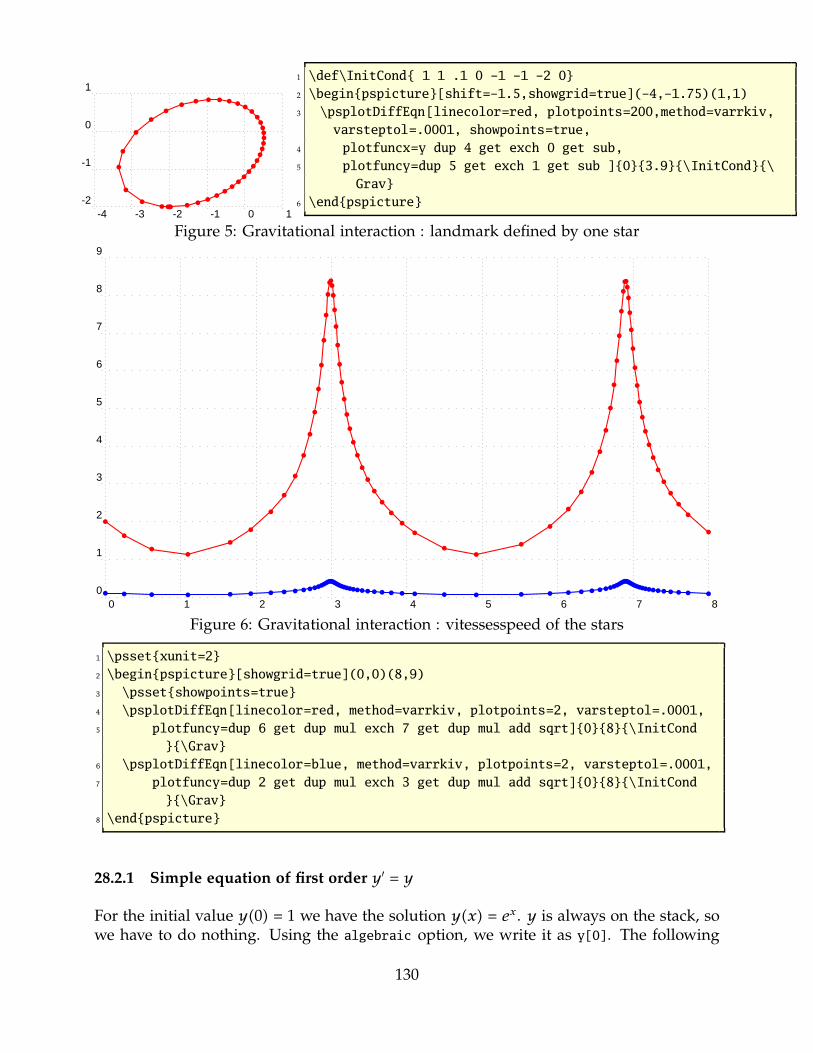
-4 -3 -2 -1 0 1-2

-1

0

1

��

�

�

�

�

�

�

��

��

��

��

��

��

1 \def\InitCond{ 1 1 .1 0 1 1 2 0}

2 \begin{pspicture}[shift=1.5,showgrid=true](4,1.75)(1,1)

3 \psplotDiffEqn[linecolor=red, plotpoints=200,method=varrkiv,

varsteptol=.0001, showpoints=true,

4 plotfuncx=y dup 4 get exch 0 get sub,

5 plotfuncy=dup 5 get exch 1 get sub ]{0}{3.9}{\InitCond}{\

Grav}

6 \end{pspicture}

Figure 5: Gravitational interaction : landmark defined by one star

0 1 2 3 4 5 6 7 80

1

2

3

4

5

6

7

8

9

�

�

��

�

�

�

�

�

�

�

�

�

�

�

�

�

��

�

�

�

�

�

�

�

�

�

�

�

�

�

�

�

�

�

�

�

�

�

�

�

�

�

�

�

�

�

�

�

�

�

��

�

�

�

�

�

�

�

�

�

�

�

�

�

�

�

�

�

� � � � � � � � � � ��

��

Figure 6: Gravitational interaction : vitessesspeed of the stars

1 \psset{xunit=2}


3 \psset{showpoints=true}

4 \psplotDiffEqn[linecolor=red, method=varrkiv, plotpoints=2, varsteptol=.0001,

5 plotfuncy=dup 6 get dup mul exch 7 get dup mul add sqrt]{0}{8}{\InitCond

}{\Grav}

6 \psplotDiffEqn[linecolor=blue, method=varrkiv, plotpoints=2, varsteptol=.0001,

7 plotfuncy=dup 2 get dup mul exch 3 get dup mul add sqrt]{0}{8}{\InitCond

}{\Grav}

8 \end{pspicture}

28.2.1 Simple equation of first order y′ = y

For the initial value y(0) = 1 we have the solution y(x) = ex. y is always on the stack, sowe have to do nothing. Using the algebraic option, we write it as y[0]. The following

130

example shows different solutions depending to the number of plotpoints with y0 = 1:

0 1 2 30123456789

10111213141516171819

Euler order 1 h = 0,2

Euler order 1 h = 0,02

RK ordre 4 h = 1

RK ordre 4 h = 0,2

solution exacte

1 \psset{xunit=4, yunit=.4}

2 \begin{pspicture}(3,19)\psgrid[subgriddiv=1]

3 \psplot[linewidth=6\pslinewidth, linecolor=green]{0}{3}{Euler x exp}

4 \psplotDiffEqn[linecolor=magenta,plotpoints=16,algebraic=true]{0}{3}{1}{y[0]}

5 \psplotDiffEqn[linecolor=blue,plotpoints=151]{0}{3}{1}{}

6 \psplotDiffEqn[linecolor=red,method=rk4,plotpoints=15]{0}{3}{1}{}

7 \psplotDiffEqn[linecolor=Orange,method=rk4,plotpoints=4]{0}{3}{1}{}

8 \psset{linewidth=4\pslinewidth}

9 \rput*(0.35,19){\psline[linecolor=magenta](.75cm,0)}

10 \rput*[l](0.35,19){\small Euler order 1 $h=0{,}2$}

11 \rput*(0.35,17){\psline[linecolor=blue](.75cm,0)}

12 \rput*[l](0.35,17){\small Euler order 1 $h=0{,}02$}

13 \rput*(0.35,15){\psline[linecolor=Orange](.75cm,0)}

14 \rput*[l](0.35,15){\small RK ordre 4 $h=1$}

15 \rput*(0.35,13){\psline[linecolor=red](.75cm,0)}

16 \rput*[l](0.35,13){\small RK ordre 4 $h=0{,}2$}

17 \rput*(0.35,11){\psline[linecolor=green](.75cm,0)}

18 \rput*[l](0.35,11){\small solution exacte}

19 \end{pspicture}

28.2.2 y′ =2 − ty

4 − t2

For the initial value y(0) = 1 the exact solution is y(x) =t +

√4 − t2

2. The function f

described in PostScript code is like (y ist still on the stack):

131

x %% y x

mul %% x*y

2 exch sub %% 2x*y

4 x dup mul %% 2x*y 4 x^2

sub %% 2x*y 4x^2

div %% (2x*y)/(4x^2)

The following example uses y0 = 1.

\newcommand{\InitCond}{1}

\newcommand{\Func}{x mul 2 exch sub 4 x dup mul sub div}

\newcommand{\FuncAlg}{(2x*y[0])/(4x^2)}

0 1 21

Euler order 1 h = 0,1Euler order 1 h = 0,01RK order 4 h = 0,19RK order 4 h = 0,095exactly

1 \psset{xunit=6.4, yunit=9.6, showpoints=false}

2 \begin{pspicture}(0,1)(2,1.7) \psgrid[subgriddiv=5]

3 { \psset{linewidth=4\pslinewidth,linecolor=lightgray}

4 \psplot{0}{1.8}{x dup dup mul 4 exch sub sqrt add 2 div}

5 \psplot{1.8}{2}{x dup dup mul 4 exch sub sqrt add 2 div} }

6 \def\InitCond{1}

7 \def\Func{x mul 2 exch sub 4 x dup mul sub div}

8 \psplotDiffEqn[linecolor=magenta, plotpoints=20]{0}{1.9}{\InitCond}{\Func}

9 \psplotDiffEqn[linecolor=blue, plotpoints=191]{0}{1.9}{\InitCond}{\Func}

10 \psplotDiffEqn[linecolor=red, method=rk4, plotpoints=11,%

11 algebraic=true]{0}{1.9}{\InitCond}{(2x*y[0])/(4x^2)}

12 \psplotDiffEqn[linecolor=Orange, method=rk4, plotpoints=21,%

13 algebraic=true]{0}{1.9}{\InitCond}{(2x*y[0])/(4x^2)}


15 \rput*(0.3,1.6){\psline[linecolor=magenta](.75cm,0)}\rput*[l](0.3,1.6){\small Euler order

1 $h=0{,}1$}

16 \rput*(0.3,1.55){\psline[linecolor=blue](.75cm,0)}\rput*[l](0.3,1.55){\small Euler order

1 $h=0{,}01$}

17 \rput*(0.3,1.5){\psline[linecolor=Orange](.75cm,0)}\rput*[l](0.3,1.5){\small RK order 4

$h=0{,}19$}

18 \rput*(0.3,1.45){\psline[linecolor=red](.75cm,0)}\rput*[l](0.3,1.45){\small RK order 4 $h

=0{,}095$}

19 \rput*(0.3,1.4){\psline[linecolor=lightgray](.75cm,0)}\rput*[l](0.3,1.4){\small exactly}

20 \end{pspicture}

132

28.2.3 y′ = −2xy

For y(−1) = 1e

we get y(x) = e−x2.

-1 0 1 2 30

1RKEuler-1solution

1 \psset{unit=4}

2 \begin{pspicture}(1,0)(3,1.1)\psgrid

3 \psplot[linewidth=4\pslinewidth,linecolor=gray]{1}{3}{Euler x dup mul neg exp

}


5 \psplotDiffEqn[linecolor=cyan]{1}{3}{1 Euler div}{x 2 mul mul}

6 \psplotDiffEqn[linecolor=yellow, method=rk4]{1}{3}{1 Euler div}{x 2 mul mul}


8 \psplotDiffEqn[linecolor=blue]{1}{3}{1 Euler div}{x 2 mul mul}

9 \psplotDiffEqn[linecolor=Orange, method=rk4]{1}{3}{1 Euler div}{x 2 mul mul}


11 \rput*(2,1){\psline[linecolor=Orange](0.25,0)}

12 \rput*[l](2,1){RK}

13 \rput*(2,.9){\psline[linecolor=blue](0.25,0)}

14 \rput*[l](2,.9){\textsc{Euler}1}

15 \rput*(2,.8){\psline[linecolor=gray](0.25,0)}

16 \rput*[l](2,.8){solution}

17 \end{pspicture}

28.2.4 Spirale of Cornu

The integrals of Fresnel :

x =

∫ t

0

cosπt2

2dt (2)

y =

∫ t

0

sinπt2

2dt (3)

133

with

x = cosπt2

2(4)

y = sinπt2

2(5)

1 \psset{unit=8}

2 \begin{pspicture}(1,1)\psgrid[subgriddiv=5]

3 \psplotDiffEqn[whichabs=0,whichord=1,linecolor=red,method=rk4,algebraic,%

4 plotpoints=500,showpoints=true]{0}{10}{0 0}{cos(Pi*x^2/2)|sin(Pi*x^2/2)}

5 \end{pspicture}

0 10

1

��

��

��

��

�

�

�

�

��

��

��

��

��

�

�

��

��

�

�

��

��

��

�

��

��

�

��

��

��

��

��

�

��

��

��

��

��

��

��

��

��

��

��

��

��

��

��

��

��

��

��

��

��

��

��

��

��

��

��

��

��

��

��

��

��

��

��

��

��

��

��

��

��

��

��

��

��

��

��

��

��

��

��

��

��

�

��

��

��

��

��

��

��

��

��

��

��

28.2.5 Lotka-Volterra

The Lotka-Volterra model describes interactions between two species in an ecosystem, apredator and a prey. This represents our first multi-species model. Since we are consid-ering two species, the model will involve two equations, one which describes how theprey population changes and the second which describes how the predator populationchanges.

For concreteness let us assume that the prey in our model are rabbits, and that thepredators are foxes. If we let R(t) and F(t) represent the number of rabbits and foxes,respectively, that are alive at time t, then the Lotka-Volterra model is:

R = a · R − b · R · F (6)

F = e · b · R · F − c · F (7)

134

where the parameters are defined by:

a is the natural growth rate of rabbits in the absence of predation,

c is the natural death rate of foxes in the absence of food (rabbits),

b is the death rate per encounter of rabbits due to predation,

e is the efficiency of turning predated rabbits into foxes.

The Stella model representing the Lotka-Volterra model will be slightly more complexthan the single species models we’ve dealt with before. The main difference is thatour model will have two stocks (reservoirs), one for each species. Each species willhave its own birth and death rates. In addition, the Lotka-Volterra model involves fourparameters rather than two. All told, the Stella representation of the Lotka-Volterramodel will use two stocks, four flows, four converters and many connectors.

-3 -2 -1 0 1 2 3 4 5 6 7 8-8

-7

-6

-5

-4

-3

-2

-1

0

1

2

3

4

5

6

7

8

9

10

��

�

�

�

�

�

�

�

�

�

�

�

�

�

�

��

�

�

�

�

�

�

�

�

�

�

�

�

�

�

��

�

�

�

�

0 1 2 3 4 5 6 7 8 9 100

1

2

3

4

5

6

7

8

9

10

11

12

13

14 �

�

�

�

�

�

�

�

�

�

�

�

�

�

�

� � � � �

�

�

�

�

�

�

�

�

�

�

�

�

�

�

�

�

�

�

�

�

� � � � � � � � � � � � � � � � � � � �

1 \def\InitCond{ 0 10 10}%% xa ya xl

2 \def\Faiglelapin{\Vaigle*(y[2]y[0])/sqrt(y[1]^2+(y[2]y[0])^2)|%

3 \Vaigle*y[1]/sqrt(y[1]^2+(y[2]y[0])^2)|%

4 \Vlapin}

135

5 \def\Vlapin{1} \def\Vaigle{1.6}

6 \psset{unit=.7,subgriddiv=0,gridcolor=lightgray,method=adams,algebraic,%

7 plotpoints=20,showpoints=true}

8 \begin{pspicture}(3,8)(5,10)\psgrid[griddots=10]

9 \psplotDiffEqn[plotfuncy=pop 0,whichabs=2,linecolor=red]{0}{10}{\InitCond}{\

Faiglelapin}

10 \psplotDiffEqn[whichabs=0,whichord=1,linecolor=black,method=rk4]{0}{10}{\

InitCond}{\Faiglelapin}

11 \psplotDiffEqn[whichabs=0,whichord=1,linecolor=blue]{0}{10}{\InitCond}{\

Faiglelapin}

12 \end{pspicture}\hfill

13 \begin{pspicture}(10,12)\psgrid

14 \psplotDiffEqn[plotfuncy=dup 1 get dup mul exch dup 0 get exch 2 get sub dup

15 mul add sqrt,linecolor=red,method=rk4]{0}{10}{\InitCond}{\Faiglelapin}

16 \psplotDiffEqn[plotfuncy=dup 1 get dup mul exch dup 0 get exch 2 get sub dup

17 mul add sqrt,linecolor=blue]{0}{10}{\InitCond}{\Faiglelapin}

18 \psplotDiffEqn[plotfuncy=pop Func aload pop pop dup mul exch dup mul add sqrt,

19 linecolor=yellow]{0}{10}{\InitCond}{\Faiglelapin}

20 \end{pspicture}

28.2.6 y′′ = y

Beginning with the initial equation y(x) = Aex + Be−x we get the hyperbolic trigonomet-rical functions.

0 1 20

1

2

3

4

5

6

7

Euler ordre 1 h = 1Euler ordre 1 h = 0,1RK ordre 4 h = 1solution exacte

1 \def\Funct{exch} \psset{xunit=5cm, yunit=0.75cm}

2 \begin{pspicture}(0,0.25)(2,7)\psgrid[subgriddiv=1,griddots=10]

3 \psplot[linewidth=4\pslinewidth, linecolor=green]{0}{2}{Euler x exp} %%e^x

4 \psplotDiffEqn[linecolor=magenta, plotpoints=11]{0}{2}{1 1}{\Funct}

5 \psplotDiffEqn[linecolor=blue, plotpoints=101]{0}{2}{1 1}{\Funct}

6 \psplotDiffEqn[linecolor=red, method=rk4, plotpoints=11]{0}{2}{1 1}{\Funct}

7 \psplot[linewidth=4\pslinewidth, linecolor=green]{0}{2}{Euler dup x exp %%ch(x

)

136

8 exch x neg exp add 2 div}




12 \psplot[linewidth=4\pslinewidth, linecolor=green]{0}{2}{Euler dup x exp

13 exch x neg exp sub 2 div} %%sh(x)




17 \rput*(1.3,.9){\psline[linecolor=magenta](.75cm,0)}\rput*[l](1.3,.9){\small\

textsc{Euler} ordre 1 $h=1$}

18 \rput*(1.3,.8){\psline[linecolor=blue](.75cm,0)}\rput*[l](1.3,.8){\small\

textsc{Euler} ordre 1 $h=0{,}1$}

19 \rput*(1.3,.7){\psline[linecolor=red](.75cm,0)}\rput*[l](1.3,.7){\small RK

ordre 4 $h=1$}

20 \rput*(1.3,.6){\psline[linecolor=green](.75cm,0)}\rput*[l](1.3,.6){\small

solution exacte}

21 \end{pspicture}

28.2.7 y′′ = −y

0 1 2 3 4 5 6 7 8 9 10 11 12 13-1

0

1

Euler order 1 h = 1Euler order 1 h = 0,1RK ordre 4 h = 1solution exacte

1 \def\Funct{exch neg}

2 \psset{xunit=1, yunit=4}

3 \def\quatrepi{12.5663706144}%%4pi=12.5663706144

137

4 \begin{pspicture}(0,1.25)(\quatrepi,1.25)\psgrid[subgriddiv=1,griddots=10]

5 \psplot[linewidth=4\pslinewidth,linecolor=green]{0}{\quatrepi}{x RadtoDeg cos

}%%cos(x)

6 \psplotDiffEqn[linecolor=blue, plotpoints=201]{0}{3.1415926}{1 0}{\Funct}

7 \psplotDiffEqn[linecolor=red, method=rk4, plotpoints=31]{0}{\quatrepi}{1 0}{\

Funct}

8 \psplot[linewidth=4\pslinewidth,linecolor=green]{0}{\quatrepi}{x RadtoDeg sin}

%%sin(x)

9 \psplotDiffEqn[linecolor=blue,plotpoints=201]{0}{3.1415926}{0 1}{\Funct}

10 \psplotDiffEqn[linecolor=red,method=rk4, plotpoints=31]{0}{\quatrepi}{0 1}{\

Funct}

11 \rput*(3.3,.9){\psline[linecolor=magenta](.75cm,0)}\rput*[l](3.3,.9){\small

Euler order 1 $h=1$}

12 \rput*(3.3,.8){\psline[linecolor=blue](.75cm,0)}\rput*[l](3.3,.8){\small Euler

order 1 $h=0{,}1$}

13 \rput*(3.3,.7){\psline[linecolor=red](.75cm,0)}\rput*[l](3.3,.7){\small RK

ordre 4 $h=1$}

14 \rput*(3.3,.6){\psline[linecolor=green](.75cm,0)}\rput*[l](3.3,.6){\small

solution exacte}

15 \end{pspicture}

28.2.8 The mechanical pendulum: y′′ = −g

lsin(y)

Pour des faibles oscillations sin(y) ≃ y:

y(x) = y0 cos

(

√

g

lx

)

The function f is writen in PostScript code:

exch RadtoDeg sin 9.8 mul %% y’ gsin(y)

138

0 1 2 3-2

-1

0

1

2

1 \def\Func{y[1]|9.8*sin(y[0])}

2 \psset{yunit=2,xunit=4,algebraic=true,linewidth=1.5pt}

3 \begin{pspicture}(0,2.25)(3,2.25)\psgrid[subgriddiv=2,griddots=10]

4 \psplot[linewidth=3\pslinewidth, linecolor=Orange]{0}{3}{.1*cos(sqrt(9.8)*x)}

5 \psset{method=rk4,plotpoints=50,linecolor=blue}

6 \psplotDiffEqn{0}{3}{.1 0}{\Func}

7 \psplot[linewidth=3\pslinewidth,linecolor=Orange]{0}{3}{.25*cos(sqrt(9.8)*x)}



10 \psplotDiffEqn{0}{3}{1 0}{\Func}

11 \psplotDiffEqn[plotpoints=100]{0}{3}{Pi 2 div 0}{\Func}

12 \end{pspicture}

28.2.9 y′′ = −y′

4− 2y

Pour y0 = 5 et y′0 = 0 la solution est :

5e−x8

(

cos (ωx) +sin(ωx)

8ω

)

avec ω =

√127

8

139

0 1 2 3 4 5 6 7 8 9 10 11 12 13 14 15 16 17 18 19 20 21 22 23 24 25 26-4

-3

-2

-1

0

1

2

3

4

5

1 \psset{xunit=.6,yunit=0.8,plotpoints=500}

2 \begin{pspicture}(0,4.25)(26,5.25)

3 \psgrid[subgriddiv=0,gridcolor=lightgray,linewidth=1.5pt]

4 \psplot[plotpoints=200,linewidth=4\pslinewidth,linecolor=gray]{0}{26}{%

5 Euler x 8 div exp x 127 sqrt 8 div mul RadtoDeg dup cos 5 mul exch sin 127

sqrt div 5 mul add mul}

6 \psplotDiffEqn[linecolor=red,linewidth=5\pslinewidth]{0}{26}{5 0}

7 {dup 3 1 roll 4 div exch 2 mul sub}

8 \psplotDiffEqn[linecolor=black,algebraic]{0}{26}{5 0} {y[1]|y[1]/42*y[0]}

9 \psset{method=rk4, plotpoints=50}

10 \psplotDiffEqn[linecolor=blue,linewidth=5\pslinewidth]{0}{26}{5 0}{%

11 dup 3 1 roll 4 div exch 2 mul sub}

12 \psplotDiffEqn[linecolor=black,algebraic=true]{0}{26}{5 0}{y[1]|y[1]/42*y

[0]}

13 \end{pspicture}

29 \psMatrixPlot

This macro allows to visualize a matrix. The datafile must be defined as a PostScriptmatrix named /dotmatrix:

/dotmatrix [ % < important line

0 1 1 0 0 0 0 1 1 1

0 1 1 0 1 1 1 0 1 0

1 0 1 1 0 0 0 1 1 0

0 0 1 0 0 0 0 0 1 1

1 1 1 1 1 0 1 0 0 1

0 0 1 1 0 1 0 1 1 1

140

1 0 0 0 1 1 0 0 0 1

0 0 0 1 1 1 0 1 1 0

1 1 0 0 0 0 1 0 0 1

1 0 1 0 0 1 1 1 0 0

] def % < important line

Important is only the value 0, in this case there happens nothing and for all other casesa dot is printed. The syntax of the macro is:

\psMatrixPlot[options]{rows}{columns}{data file}

The matrix is scanned line by line from the the first one to the last. In general it looksvice versa than the above listed matrix, the first row 0 1 1 0 0 0 0 1 1 1 is the first plottedline (y = 1). With the option ChangeOrder=true it looks exactly like the above view.

0

1

2

3

4

5

6

7

8

9

10

0 1 2 3 4 5 6 7 8 9 10

��

��

� ��

��

� � � � � �

� � � � �

� � �

� � � � � � �

� � � � � �

� � � �

� � � � �

� � � �

� � � � �

1 \begin{pspicture}(0.5,0.75)(11,11)

2 \psaxes{>}(11,11)

3 \psMatrixPlot[dotsize=1.1cm,dotstyle=square*,linecolor=magenta]%

4 {10}{10}{matrix.dat}

5 \psMatrixPlot[dotsize=.5cm,dotstyle=o,ChangeOrder]{10}{10}{matrix.dat}

6 \end{pspicture}

141

0

1

2

3

4

5

6

7

8

9

10

0 1 2 3 4 5 6 7 8 9 10

� � �

� � � � � �

� � � � �

� �

� � �

� � � � � �

� � � �

� � � �

� � �

� � � � �

1 \begin{pspicture}(0.5,0.75)(11,11)

2 \psaxes{>}(11,11)

3 \psMatrixPlot[dotscale=3,dotstyle=*,linecolor=blue]{10}{8}{matrix.dat}

4 \end{pspicture}

30 \psforeach

The macro \psforeach allows a loop with an individuell increment.

\psforeach{variable}{value list}{action}

0 1 2 3 4 50

1

2

3

4

5

�

�

�

�

�

1 \begin{pspicture}[showgrid=true](5,5)

2 \psforeach{\nA}{0, 1, 1.5, 3, 5}{%

3 \psdot[dotscale=3](\nA,\nA)}

4 \end{pspicture}

142

31 \resetOptions

Sometimes it is difficult to know what options, which are changed inside a long docu-ment, are different to the default one. With this macro all options depending to pstplot

can be reset. This depends to all options of the packages pstricks, pstplot and pstnode.

A PostScript

PostScript uses the stack system and the LIFO system, "’Last In, First Out"‘.

FunctionMeaning

on stack before → after

add x y → x + ysub x y → x − ymul x y → x × ydiv x y → x ÷ ysqrt x → √

xabs x → |x|neg x → −xcos x → cos(x) (x in degrees)

sin x → sin(x) (x in degrees)

tan x → tan(x) (x in degrees)

atan y x → 6 ( ~Ox; ~OM) (in degrees of M(x, y))ln x → ln(x)log x → log(x)array n → v (of dimension n)aload v → x1 x2 · · · xn vastore x1 x2 · · · xn v → vpop x →dup x x →roll x1 x2 · · · xn np →

Table 5: Some primitive PostScript macros

B Credits

Hendri Adriaens | Martin Chicoine | Ulrich Dirr | Hubert Gäßlein | Denis Girou| Peter Hutnick | Christophe Jorssen | Uwe Kern | Manuel Luque | Jens-UweMorawski | Tobias Nähring | Rolf Niepraschk | Alan Ristow | Arnaud Schmittbuhl |Timothy Van Zandt

143

References

[1] Hendri Adriaens. xkeyval package. CTAN:/macros/latex/contrib/xkeyval, 2004.

[2] Denis Girou. Présentation de PSTricks. Cahier GUTenberg, 16:21–70, April 1994.

[3] Michel Goosens, Frank Mittelbach, and Alexander Samarin. The LATEX GraphicsCompanion. Addison-Wesley Publishing Company, Reading, Mass., 1997.

[4] Alan Hoenig. TEX Unbound: LATEX & TEX Strategies, Fonts, Graphics, and More.Oxford University Press, London, 1998.

[5] Laura E. Jackson and Herbert Voß. Die plot-funktionen von pstplot. DieTEXnische Komödie, 2/02:27–34, June 2002.

[6] Nikolai G. Kollock. PostScript richtig eingesetzt: vom Konzept zum praktischen Einsatz.IWT, Vaterstetten, 1989.

[7] Frank Mittelbach and Michel Goosens et al. The LATEX Graphics Companion.Addison-Wesley Publishing Company, Boston, second edition, 2004.

[8] Frank Mittelbach and Michel Goosens et al. Der LATEX Begleiter. Pearson Education,München, zweite edition, 2005.

[9] Herbert Voß. Chaos und Fraktale selbst programmieren: von Mandelbrotmengen überFarbmanipulationen zur perfekten Darstellung. Franzis Verlag, Poing, 1994.

[10] Herbert Voß. Die mathematischen Funktionen von PostScript. Die TEXnischeKomödie, 1/02, March 2002.

[11] Herbert Voß. PSTricks Grafik für TEX und LATEX. DANTE – Lehmanns,Heidelberg/Hamburg, third edition, 2006.

[12] Herbert Voß. LATEX in Naturwissenschaften & Mathematik. Franzis Verlag, München,first edition, 2006.

[13] Timothy Van Zandt. PSTricks - PostScript macros for generic TEX.http://www.tug.org/application/PSTricks, 1993.

[14] Timothy Van Zandt. multido.tex - a loop macro, that supports fixed-point addition.CTAN:/graphics/pstricks/generic/multido.tex, 1997.

[15] Timothy Van Zandt. pstplot: Plotting two dimensional functions and data.CTAN:graphics/pstricks/generic/pstplot.tex, 1999.

[16] Timothy Van Zandt and Denis Girou. Inside PSTricks. TUGboat, 15:239–246,September 1994.

144

CTAN:/macros/latex/contrib/xkeyval

http://www.tug.org/application/PSTricks

CTAN:/graphics/pstricks/generic/multido.tex

CTAN:graphics/pstricks/generic/pst-plot.tex

C Change log

See file Changes

145

additionals Macros for pstricks

Documents

Transcript of additionals Macros for pstricks