PLP 937

January 1985

ADDITIONAL ENGINEERING DATA ON TOKAPOLE II

J.e. Sprott

J.S. Sarff

Plasma Studies

University of Wisconsin

These PLP Reports are informal and preliminary and as such may contain errors not yet eliminated. They are for private

circulation only and are not to be further transmitted without

consent of the authors and major professor.

ADDITIONAL ENGINEERING DATA ON TOKAPOLE II

J.C. Sprott and J.S. Sarff

On May 17, 1984 the upper inner hanger at 600 on Tokapole II was broken

during normal pulsing. This provided both a reason and an opportunity to

measure more precisely some of the electrical and mechanical properties of

the machine in order to better quantify operational limits and expected Hfe

of various components. This note contains a summary of these measurements.

-2-

I. Hoop and Hanger Stresses

The stresses acting on the hoops and their hangers during a magnetic

field pulse are described in PLP 744. In the original design, no

consideration was given to the time dependence of the forces other than to

allow an additional safety factor of 1.7 for a half-sine-wave excitation of

the worst possible frequency (see PLP 30). This frequency turns out to be

twice the natural resonant frequency of the mechanical systemt since the

force is proportional to the square of the magnetic field. The natural

frequencies and Qls of the various mechanical modes have been measured.

The technique for measuring vibrations of the hoops consists of biasing

the hoop under test to �67 volts using a battery and series 10 kg resistor

for current limiting. An electrode of vI cm2

area is then placed vI mm from

the hoop and connected to a I MO input oscilloscope. The displacement

appears as a voltage signal through the relation

= R V dC

input bias dt

where C is the capacitance between the electrode and the h�op

(vlO-12 farads). The signal is typically Vout S 1 mV, and thus careful

shielding and bandpass filtering are required to reduce noise and pickup

(especially 60 Hz). The oscillations can be excited either by tapping the

hoop with a hammer or by pulsing the field at low amplitude (typically a

single, 240 �F capacitor was usedt charged to 4 kV, with no crowbar). The

various modes can be distinguished by the method of excitation and by the

- 3 -

toroidal location of the detector. Signal-to-noise ratio is tested by

reversing the bias polarity and triggering the scope on the driving

excitation. Figure 1 shows a typi�al output signal. The measurements were

subsequently retaken with a piezoelectric accelerometer with similar

results.

The hoo p/hanger system has several modes in which it can oscillate.

These are most conveniently catalogued by specifying their toroidal mode

number n, where the amplitude of the displacement is assumed to vary as ein�

and � is the toroidal angle. The simplest (and most important from the

standpoint of hanger stress) is n = 0 which is strongly driven by the normal

method of excitation. It simply represents a longitudinal vibration of the

hangers coupled to a mass equal to the portion of the hoop that they support

(one-third).

Modes with n > 0 can be excited by striking the hoop at an appropriate

location with a hammer. The modes which are most strongly excited by thls

method are those for which n is a multiple of 6 (n = 6, 12, 18, . • • ) since

the hangers act as nodes and the periodic boundary condition does not allow

multiples of 3. The n = 6 mode is overwhelmingly the most dominant, and it

oscillates with a large amplitude and extremely high Q. During normal

pulsing of the machine, this mode is not excited, however, because of the

symmetry of the driving force.

For normal excitation, the dominant mode has n = 3 and involves a sharp

bending of the hoop at the supports. This is the mode that is considered in

PLP 744, and is the most serious candidate for breaking the hoops. It is

this mode that ultimately lead to the death of Tokapole I after 15 years of

- 4 -

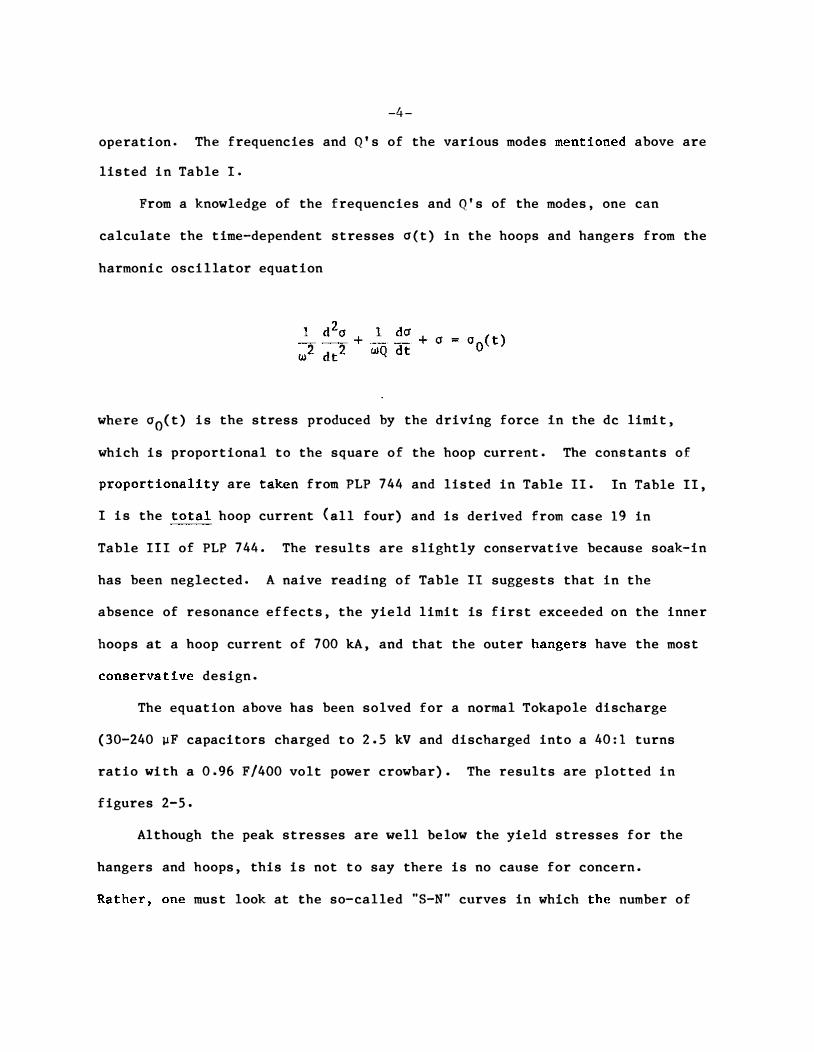
operation. The frequencies and Q's of the various modes mentioned above are

listed in Table I.

From a knowledge of the frequencies and Q's of the modes, one can

calculate the time-dependent stresses a(t) in the hoops and hangers from the

harmonic oscillator equation

where 00(t) is the stress produced by the driving force in the dc limit,

which is proportional to the square of the hoop current. The constants of

proportionality are taken from PLP 744 and listed in Table II. In Table II,

I is the to!al hoop current (all four) and is derived from case 19 in

Table III of PLP 744. The results are slightly conservative because soak-in

has been neglected. A naive reading of Table II suggests that in the

absence of resonance effects, the yield limit is first exceeded on the inner

hoops at a hoop current of 700 kA, and that the outer hangers have the most

conservative design.

The equation above has been solved for a normal Tokapole discharge

(30-240 �F capacitors charged to 2.5 kV and discharged into a 40:1 turns

ratio with a 0.96 F/400 volt power crowbar). The results are plotted in

figures 2-5.

Although the peak stresses are well below the yield stresses for the

hangers and hoops, this is not to say there is no cause for concern.

Rather, one must look at the so-called "S-N" curves in which the number of

-5-

cycles to failure is plotted vs the stress. Unfortunately, such curves are

not available for the copper alloys used in Tokapole II. However, a curve

for a similar hardened, malleable, copper alloy taken from Russell and

Welcker, Proc. Am. Soc. Test. Mat., 36 118 (1936) is shown in figure 6 .

Although there is some scatter in the data, a reasonable fit is

12.5 0 /0 N = 0.36 e y

In estimating the number of machine pulses to expect before failure,

one has to consider the fact that each machine pulse results in a succession

of stress peaks as the mechanical system oscillates. If the oscillations

have sufficiently high Q, the number of pulses before failure is reduced by

a factor of v12.5 �Oy/Qop where 0p is the peak stress during the first cycle

of oscillation. Unless Q considerably exceeds 12.5 �a /0 , which is usually y p

not the case for Tokapole II, this factor can be ignored.

On the basis of these considerations, one can estimate the number of

pulses before failure for various hoop currents, obtained by raising and

lowering the voltage on the Bp capacitor bank. The results are sho"m in

Table III. The implication of these numbers is that the observed failure

was probably not a normal fatigue failure, but rather indicates a flaw

(scratch, etc. ) in the material.

- 6 -

II. Poloidal Field Circuit Losses

When the poloidal field capacitor bank is discharged into the Tokapole,

some of the energy is lost resistively in the transmission line. ignitron,

primary windings, continuity windings, and walls of the machine, and some is

stored inductively in the transmission line and in leakage inductance in the

iron core. Some of these losses were predicted in PLP 744, but most have

never been measured carefully. We report here the results of such

measurements.

Figure 7 shows the poloidal field circuit and the measured values of

the various circuit elements. These measurements were made using a

carefully calibrated pair of XlO,OOO attenuators (500 kn to 50 Q) connected

to the differential input of a Tektronix 466 oscilloscope. The inductive

components come from early-time measurements, before the current has risen

significantly, and the resistive components are from later in the pulse

after the current has risen to near its peak value.

The V-I characteristic of the class E, BT crowbar ignitron was measured

and is plotted in figure 8. The voltage, over the range of currents of

interest, is remarkably constant at .... 10-16 volts, which probably represents

the sum of the work function of the cathode (4.5 volts) plus the ionization

potential of mercury (10.44 volts). There is also a slight tendency for the

voltage drop to decrease in time during the pulse. especially at low

currents.

-7-

The dc resistance of the hoops is calculated to be Rl = 24.823 �Q for

each inner hoop and R2 = 44.798 �Q for each outer hoop. At very late times

(t » L/R v 27 msec), the hoops all appear in parallel, and the net

resistance is 7.98 �n. At early times (t « L/R v 27 msec), the currents

divide inductively, and the equivalent series dc resistance is

where 1'1 = 0.688 �H and L2 = 1.2 \.IH are the inductances of the inner and

outer hoops respectively (from case 19 PLP 744). The ac resistance of. the

hoops has been calculated by Kerst in PLP 893 . His results, fitted to an

exponential function of time over the range 1-20 msec give

His results are strictly valid only for a step function hoop current, but

probably are not unreasonable for our case with a power crowbar. Putting it

all together gives

R = 8.0 + 10.0 e-420t \.In

�-

III. Toroidal Field Circuit Losses

In similar fashion, the toroidal field circuit losses have been

measured, and the results were reported in PLP 924.

- 9 -

Table I

Frequencies and Q's of the normal modes of vibration of the Tokapole II

hoops.

n

o

3

6

n

o

3

6

f

29.5 Hz

180 Hz

430 Hz

f

290 Hz

180 Hz

430 Hz

UPPER INNER

45

50

1.2 x 104

Lm-lER INNER

70

50

1.2 x 104

n

o

3

6

n

o

3

6

UPPER OUTER

f

280 Hz

70 Hz

130 Hz

30

125

2 x 104

I,OWER OUTER

f

310 Hz

70 Hz

130 Hz

30

125

2 x 104

-10-

Table II

Stress Coefficients for Tokapole II

Stress/MA2 Yield Stress

(Oo/I2

) (Oy

)

Outer hanger 12.8 kpsi/MA2 165 kpsi

Inner hanger 184 kpsi/MA2 165 kpsi

Outer hoop 67 kpsi/MA2 43 kpsi

Inner hoop 89 kpsi/�..A2 43 kpsi

-11-

Tahle III

Estimated Fatigue Life of Various Components of Tokapole II

Hoop current 270 kA 390 kA 520 kA 650 kA

Outer hanger

Inner hanger 1042

Outer hoop

Inner hoop

Fig. 1: A typical output signal using the displacement current technique or

a piezoelectric acclerometer. This case is the hammer-struck n = 3

mode for the lower outer hoop.

-50

I I

-

I I

OUTER HANGER STRESS (KPSI)

!

• •

• • •

• •

•

•

• »

I

•

• •

•

• •

•

50

I I I

-

-

-

-

t I !

TOKAPOLE II/TOK WITH N = 40 TURNS, C - 7.2E-03 FARADS, 20 MSEC FULL SCALE

INITIAL CAPACITOR VOLTAGE = 2500 VOLT-SECONDS CONSUMED = .070537

CORE BIAS = 0 KG ( .268 AMP-TURNS) PRIMARY RESISTANCE = .0485 OHMS

INITIAL PLASMA RESISTANCE = .01 OHMS CROWBAR VOLTAGE = 400

Fig. 2

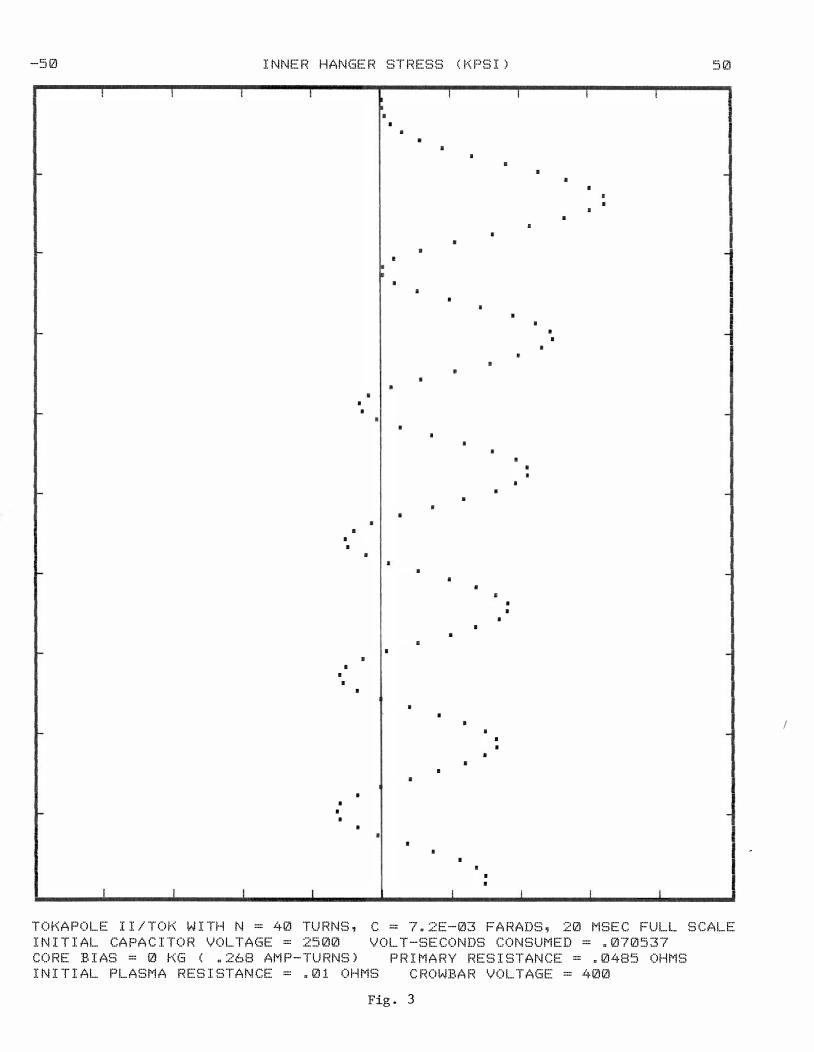
-50

I I I

-

I I

INNER HANGER STRESS (KPSI)

I

I

•

• •

•

• • •

• •

•

•

•

� •

I

•

•

•

•

I

•

• •

• •

• •

I

I

• •

I

i

50

-

-

-

I

I C = 7.2E-03 FARADS, 20 MSEC FULL SCALE

VOLT-SECONDS CONSUMED = .070537

PRIMARY RESISTANCE = .0485 OHMS

TOKAPOLE II/TOK WITH N = 40 TURNS,

INITIAL CAPACITOR VOLTAGE = 2500

CORE BIAS = 0 KG ( . 268 AMP-TURNS)

INITIAL PLASMA RESISTANCE = .01 OHMS CROWBAR VOLTAGE = 400

Fig. 3

I

-50

! I

I ! I

OUTER HOOP STRESS (KPSI)

I

I

• • • •

• •

• •

•

• •

• •

• •

•

•

• •

•

•

• •

t

•

• •

•

•

I

50

t I

f

� �

& -

� � �

�

-

-

-

-

-

I I I

TOKAPOLE II/TOK WITH N = 40 TURNS,

INITIAL CAPACITOR VOLTAGE = 2500

{� -w - 7.2E-03 FARADS� 20 MSEC FULL SCALE

VOLT-SECONDS CONSUMED = .070537

PRIMARY RESISTANCE = .0485 OHMS CORE BIAS = 0 KG ( .268 AMP-TURNS)

INITIAL PLASMA RESISTANCE = .01 OHMS CROWBAR VOLTAGE = 400

Fig. 4

-5�

I I I

j ! I

INNER HOOP STRESS (KPSI)

I

!

• •

•

• I

• •

•

•

•

I

•

•

!

• • •

• •

• •

•

• •

50

I

-

-

-

-

-

-

I

TOKAPOLE II/TOK WITH N = 4� TURNS, C =

INITIAL CAPACITOR VOLTAGE = 25�0 7.2E-�3 FARADS, 2� MSEC FULL SCALE

VOLT-SECONDS CONSUMED = .070537 PRIMARY RESISTANCE = .0485 OHMS CORE BIAS = 0 KG ( .268 AMP-TURNS)

INITIAL PLASMA RESISTANCE = .01 OHMS CROWBAR VOLTAGE = 400

Fig. 5

�------�--------�--------�-------'---------r--------' � <:>

� b3} ,.. in 0

.

at

Q} \D �

.. llJ () �

� :::> -.J

:E '"

<:)

0 -

() \-

1.0

(I) Z 00 'r-! UJ �

r:I.. ..... \)

W "> 0 0 a.. \) Q.. \I)

0 () U lL..

0

@ 0 �

w UJ co

0 r.. i UJ ':) 0 z Q!

- a: � en :J:. � 0 Q) L

.... lJ)

-0

b3') .!l :n

-

rc} ()

0 0 0 0 0 0 0 '-D \.c) .::l- M <U

R, L,

C, ... I

C1 = 0.0072 F

R1 6 mn

L1 = 4.5 J,lH

Rn = 61 mn

LD = 2.5 J,lH

Cz = 0.96 F

R2 = 4 mn

L '" 0 2

LD o

Vey

'-.../ �3

V.

R2

� L2 ,-

Ca +

VI = 14 V

V2 = 68 V

R3 = 3 mn

L3 = 3 J,lH

R4 = 17 mn N = @ 40

70 mn N = @ 80

L4 = 16 J,lH N = @ 40

70 J,lH N = @ 80

RS = 2J,ln

Fig. 7: Circuit parameters of:poloidal field circuit.

L3

I I Rs .-. • I �

VPG

'" : ,

+

+

2 Q � \-:z

\!:J

ill

� (( -.I

U

+

o

N

+

0

0

0 0

0

+

0

+

+ 0

+

0

+

0

+. 0

+

0

0

4- 0

0

0

+

0

0

0

III '" ..l � Cl.

%

� Q£ (( III

...

0

+

+ 0

0

� 00

0

0

0 0 0

0 0

0

0

\U

U\ .J ;:) Q.

Z

\U t-« oJ

0

� ru

0 N

cO

'-0

.::t-

(\J

<:)

00

o o

� � co

C( a 00

-M -l �

�