'

&

$

%

ADAPTIVITY IN CLINICAL TRIAL DESIGNS:

OLD AND NEW

Christopher Jennison,

Dept of Mathematical Sciences, University of Bath, UK

and

Bruce Turnbull,

Cornell University, Ithaca, New York

London 2 December 2004

c©2004 Jennison, Turnbull

1

'

&

$

%

0. A Cautionary Tale

Class action lawsuit vs Fred Hutchinson Cancer Center, Seattle.

Protocol 126: Bone marrow transplant for leukemia, 1981–1993

Civil trial: Feb-April 2004.

Plaintiffs: Estates of 5 deceased subjects.

Attorney: Alan Milstein — well-known scourge of clinical trialists including

IRB and DSMB members (successful cases vs U. Penn, U. Oklahoma, . . . )

Charges: breach of the right to dignity, fraud, assault and battery, product

liability, violations of laws governing research and consumer rights.

2

'

&

$

%

Protocol 126

Of concern to us: Statements made by plaintiff’s expert statistical witness

1. Phase 1: Sample size was 12, but no rationale given in protocol or SAP.

Actual sample size was 22 — no documentation for change, nor any approval

by IRB.

“Unexplained change was substandard, because once you state the

sample size you should abide by it.”

2. Phase 3: No formal plan for interim monitoring or stopping rules in protocol.

Only “vague” statement that study would be stopped if there was

“cumulative evidence of toxicity or lack of efficacy”

3. There was enough statistical evidence at a meeting on Feb 8, 1984 to

warrant stopping the trial, which would have saved the enrollment of 50

additional subjects.

4. Relapse-free survival curves to be used to calculate monetary damages.

3

'

&

$

%

Protocol 126

Note: In 1983, President of Fred Hutchinson Cancer Center turned down a

request from IRB to establish an independent DSMB on the grounds of

cost and that it would “reveal secrets to competitors”.

Now we have:

• FDA (1998) Guidance for Industry: E9 Statistical Principles for Clinical

Trials

• FDA (2001) Draft Guidance for Clinical Trial Sponsors: On the

Establishment and Operation of Clinical Trial Data Monitoring

Committees.

4

'

&

$

%

Adaptivity

• Adaptive choice of test statistic as information on assumptions

emerge; e.g. adaptive scores in a linear rank test, logrank vs Gehan

• Adaptive allocation to achieve balance within strata

• Adaptive allocation to assign fewer patients to inferior treatment arm

• Adaptivity to accruing information on nuisance parameters

• Adaptivity to accruing information on safety/secondary endpoints

• Adaptivity to adjust power based on accruing information on primary

endpoints

• Adaptivity to to drop arms in multi-arm study based on accruing

information on primary endpoints

• Others ....

5

'

&

$

%

Outline of Presentation

1. Interim monitoring of clinical trials

Adapting to observed data

2. Distribution theory, the role of “information”

3. Error-spending tests

Adapting to unpredictable information

Adapting to nuisance parameters

4. Most efficient group sequential tests

Adapting optimally to observed data

5. More recent adaptive proposals

6. Example of inefficiency in an adaptive designs

7. Conclusions

6

'

&

$

%

1. Interim monitoring of clinical trials

It is standard practice to monitor progress of clinical trials for reasons of

ethics, administration (accrual, compliance) and economics.

Special methods are needed since multiple looks at accumulating data can

lead to over-interpretation of interim results

Methods developed in manufacturing production were first transposed to

clinical trials in the 1950s.

Traditional sequential methods assumed continuous monitoring of data,

whereas it is only practical to analyse a clinical trial on a small number of

occasions.

The major step forward was the advent of Group Sequential methods in

the 1970s.

7

'

&

$

%

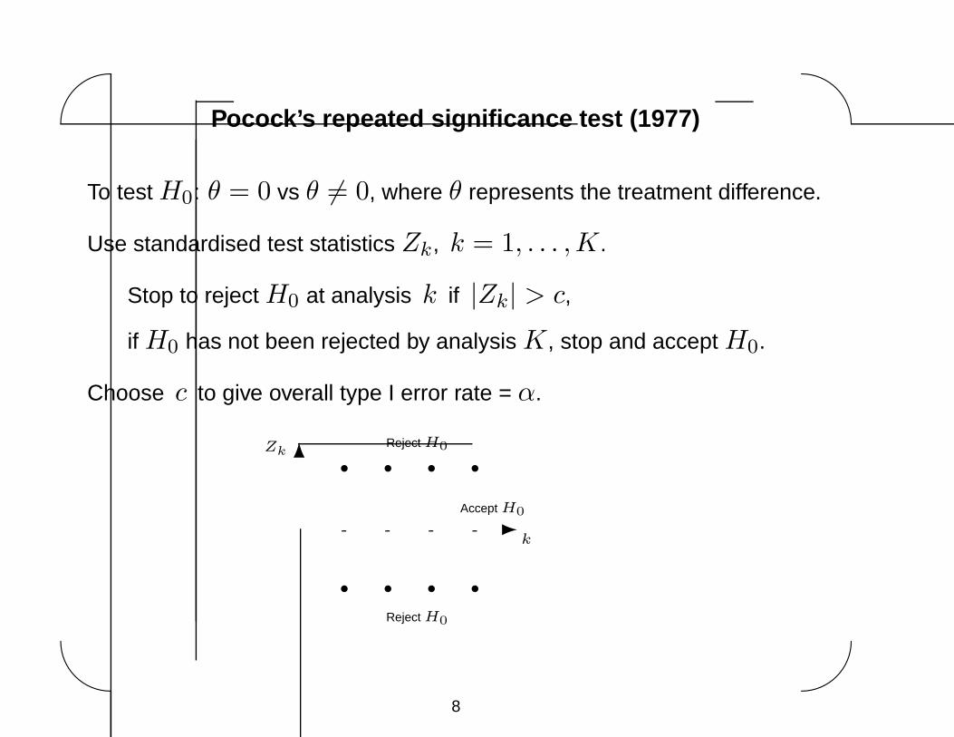
Pocock’s repeated significance test (1977)

To test H0: θ = 0 vs θ 6= 0, where θ represents the treatment difference.

Use standardised test statistics Zk, k = 1, . . . ,K .

Stop to reject H0 at analysis k if |Zk| > c,

if H0 has not been rejected by analysis K , stop and accept H0.

Choose c to give overall type I error rate = α.

-k

6Zk

• • • •

• • • •

Reject H0

Reject H0

Accept H0

8

'

&

$

%

Types of hypothesis testing problems

Two-sided test:

testing H0: θ = 0 against θ 6= 0.

One-sided test:

testing H0: θ ≤ 0 against θ > 0.

Equivalence tests:

one-sided — to show treatment A is as good

as treatment B, within a margin δ (non-inferiority).

two-sided — to show two treatment formulations

are equal within an accepted tolerance.

9

'

&

$

%

Types of early stopping

1. Stopping to reject H0: No treatment difference

• Allows progress from a positive outcome

• Avoids exposing further patients to the inferior treatment

• Appropriate if no further checks are needed on

treatment safety or long-term effects.

2. Stopping to accept H0: No treatment difference

• Stopping “ for futility” or “abandoning a lost cause”

• Saves time and effort when a study is unlikely to

lead to a positive conclusion.

10

'

&

$

%

One-sided tests

To look for superiority of a new treatment, test

H0: θ ≤ 0 against θ > 0.

If the new treatment if not effective, it is not appropriate to keep sampling

to find out whether θ = 0 or θ < 0.

Specify type I error rate and power

Pr{Reject H0 | θ = 0} = α,

Pr{Reject H0 | θ = δ} = 1 − β.

A sequential test can reduce expected sample size under θ = 0, θ = δ,

and at effect sizes in between.

11

'

&

$

%

One-sided tests

A typical boundary one-sided testing boundary:

-k

6Zk

•

•

• • •

•

•

•

•

PP`

��

""

!!

!!

Reject H0

Accept H0

E(Sample size) can be around 50 to 70% of the fixed sample size

— adapting to data, stopping when a decision is possible.

12

'

&

$

%

2. Joint distribution of parameter estimates

Let θk be the estimate of the parameter of interest, θ, based on data at

analysis k.

The information for θ at analysis k is

Ik =1

Var(θk), k = 1, . . . ,K.

Canonical joint distribution of θ1, . . . , θK

In very many situations, θ1, . . . , θK are approximately multivariate

normal,

θk ∼ N(θ, {Ik}−1), k = 1, . . . ,K,

and

Cov(θk1, θk2

) = Var(θk2) = {Ik2

}−1 for k1 < k2.

13

'

&

$

%

Canonical joint distribution of z-statistics

In a test of H0: θ = 0, the standardised statistic at analysis k is

Zk =θk√

Var(θk)= θk

√Ik.

For this,

(Z1, . . . , ZK) is multivariate normal,

Zk ∼ N(θ√Ik, 1), k = 1, . . . ,K ,

Cov(Zk1, Zk2

) =√Ik1

/Ik2for k1 < k2.

14

'

&

$

%

Canonical joint distribution of score statistics

The score statistics Sk = Zk√Ik , are also multivariate normal with

Sk ∼ N(θ Ik, Ik), k = 1, . . . ,K.

The score statistics possess the “independent increments” property,

Cov(Sk − Sk−1, Sk′ − Sk′−1) = 0 for k 6= k′.

It can be helpful to know the score statistics behave as Brownian motion

with drift θ observed at times I1, . . . , IK .

15

'

&

$

%

Sequential distribution theory

The preceding results for the joint distribution of θ1, . . . , θK can be

demonstrated directly for:

θ a single normal mean,

θ = µA − µB, the effect size in a comparison of two normal means.

The results also apply when θ is a parameter in:

a general normal linear,

a general model fitted by maximum likelihood (large sample theory).

So, we have the theory to support general comparisons, including

adjustment for covariates if required.

16

'

&

$

%

Survival data

The canonical joint distributions also arise for:

parameter estimates in Cox’s proportional hazards regression model

a sequence of log-rank statistics (score statistics) for comparing two

survival curves

— and to z-statistics formed from these.

For survival data, observed information is roughly proportional to the

number of failures seen.

Special types of group sequential test are needed to handle unpredictable

and unevenly spaced information levels.

17

'

&

$

%

3. Error spending tests

Lan & DeMets (Biometrika, 1983) presented two-sided tests which “spend”

type I error probability as a function of observed information.

The error spending function, f(I), gives the type I error probability to be

spent up to the current analysis

-IkImax

6f(I)

α

��!!��""��

����

""��!!��

18

'

&

$

%

Maximum information design

• Specify the error spending function f(I)

• For each k = 1, 2, . . . , set the boundary at analysis k to give

cumulative type I error probability f(Ik).

• Accept H0 if Imax is reached without rejecting H0.

Precise rules are available to protect the type I error rate if the information

sequence over-runs the target Imax, or if the study ends without reaching

reaching this target. See slides 23 and 24 or Chapter 7 of Jennison &

Turnbull (2000).

19

'

&

$

%

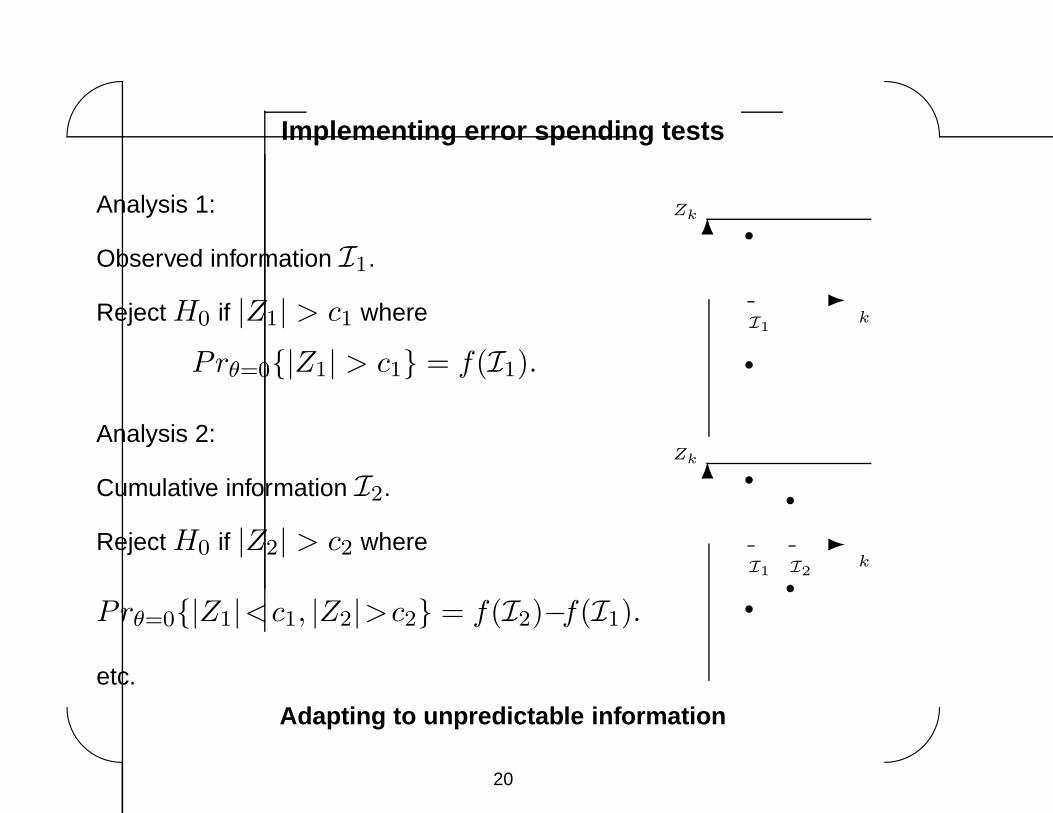
Implementing error spending tests

Analysis 1:

Observed information I1.

Reject H0 if |Z1| > c1 where

Prθ=0{|Z1| > c1} = f(I1).

-I1

k

6Zk

•

•

Analysis 2:

Cumulative information I2.

Reject H0 if |Z2| > c2 where

Prθ=0{|Z1|<c1, |Z2|>c2} = f(I2)−f(I1).

-I1 I2

k

6Zk

•

•

•

•

etc.

Adapting to unpredictable information

20

'

&

$

%

One-sided error spending tests

Define f(I) and g(I) for spending type I and type II error probabilities.

-IImax

6f(I)

α

������

�����

-IImax

6g(I)

β

������

�����

At analysis k, set boundary values (ak, bk) so that

Prθ=0 {Reject H0 by analysis k} = f(Ik),

P rθ=δ {Accept H0 by analysis k} = g(Ik).

Power family of error spending tests: f(I) and g(I) ∝ (I/Imax)ρ.

21

'

&

$

%

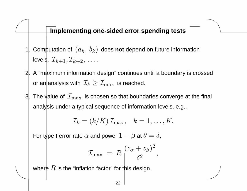
Implementing one-sided error spending tests

1. Computation of (ak, bk) does not depend on future information

levels, Ik+1, Ik+2, . . . .

2. A “maximum information design” continues until a boundary is crossed

or an analysis with Ik ≥ Imax is reached.

3. The value of Imax is chosen so that boundaries converge at the final

analysis under a typical sequence of information levels, e.g.,

Ik = (k/K) Imax, k = 1, . . . ,K.

For type I error rate α and power 1 − β at θ = δ,

Imax = R(zα + zβ)2

δ2,

where R is the “inflation factor” for this design.

22

'

&

$

%

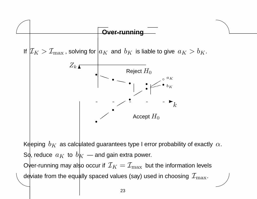
Over-running

If IK > Imax , solving for aK and bK is liable to give aK > bK .

-k

6Zk

•

•

• • • bK

◦aK

•

•

•

•

PP`

��

""

""

""........

Reject H0

Accept H0

Keeping bK as calculated guarantees type I error probability of exactly α.

So, reduce aK to bK — and gain extra power.

Over-running may also occur if IK = Imax but the information levels

deviate from the equally spaced values (say) used in choosing Imax.

23

'

&

$

%

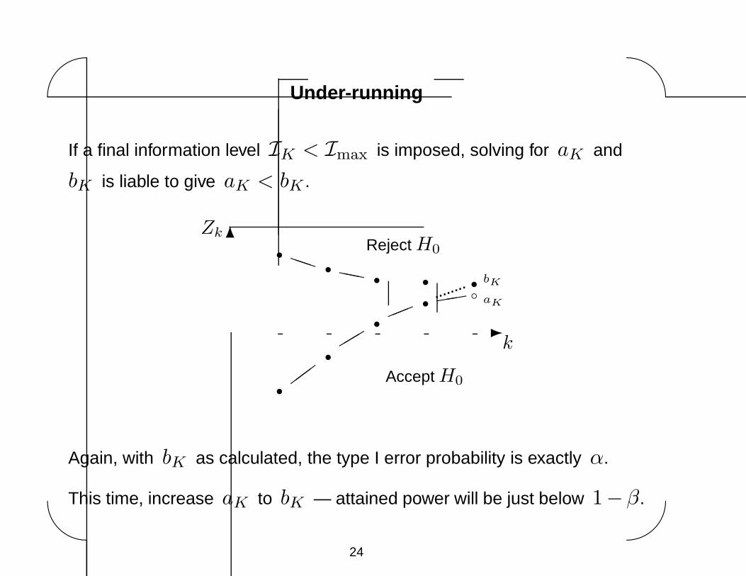
Under-running

If a final information level IK < Imax is imposed, solving for aK and

bK is liable to give aK < bK .

-k

6Zk

•

•

• • •bK

◦ aK•

•

•

•

PP`

��

""

!!((........

Reject H0

Accept H0

Again, with bK as calculated, the type I error probability is exactly α.

This time, increase aK to bK — attained power will be just below 1−β.

24

'

&

$

%

Error-spending designs and nuisance parameters

(1) Survival data, log-rank statistics

Information depends on the number of observed failures,

Ik ≈ 1

4{Number of failures by analysis k}.

With fixed dates for analyses, continue until information reaches Imax.

-×I1

×I2

×I3

×I4

×I5

×I6

Imax

Information

If the overall failure rate is low or censoring is high, one may decide to

extend the patient accrual period.

Changes affecting {I1, I2, . . . } can be based on observed information;

they should not be influenced by the estimated treatment effect.

25

'

&

$

%

Error-spending designs and nuisance parameters

(2) Normal responses with unknown variance

In a two treatment comparison, a fixed sample test with type I error rate α

and power 1 − β at θ = δ requires information

If =(zα + zβ)2

δ2.

A group sequential design with inflation factor R needs maximum

information Imax = R If .

The maximum required information is fixed — but the sample size needed

to provide this level of information depends on the unknown variance σ2.

Adapting to nuisance parameters

26

'

&

$

%

Adjusting sample size as variance is estimated

The information from nA observations on treatment A and nB on B is

I =

{(1

nA+

1

nB

)σ2

}−1

.

Initially: Set maximum sample sizes to give information Imax if σ2 is

equal to an initial estimate, σ20 .

As updated estimates of σ2 are obtained: Adjust future group sizes so

the final analysis has{(

1

nA+

1

nB

)σ2

}−1

= Imax.

NB, state Imax in the protocol, not initial targets for nA and nB .

At interim analyses, apply the error spending boundary based on observed

(estimated) information.

27

'

&

$

%

4. Optimal group sequential tests

“Optimal” designs may be used directly — or they can serve as a

benchmark for judging efficiency of designs with other desirable features.

Optimising a group sequential test:

Formulate the testing problem:

fix type I error rate α and power 1 − β at θ = δ,

fix number of analyses, K ,

fix maximum sample size (information), if desired

Find the design which minimises average sample size (information) at

one particular θ or averaged over several θ s.

28

'

&

$

%

Derivation of optimal group sequential tests

Create a Bayes decision problem with a prior on θ, sampling costs and

costs for a wrong decision. Write a program to solve this Bayes problem by

backwards induction (dynamic programming).

Search for a set of costs such that the Bayes test has the desired

frequentist properties: type I error rate α and power 1 − β at θ = δ.

This is essentially a Lagrangian method for solving a constrained

optimisation problem — the key is that the unconstrained Bayes problem

can be solved accurately and quickly.

29

'

&

$

%

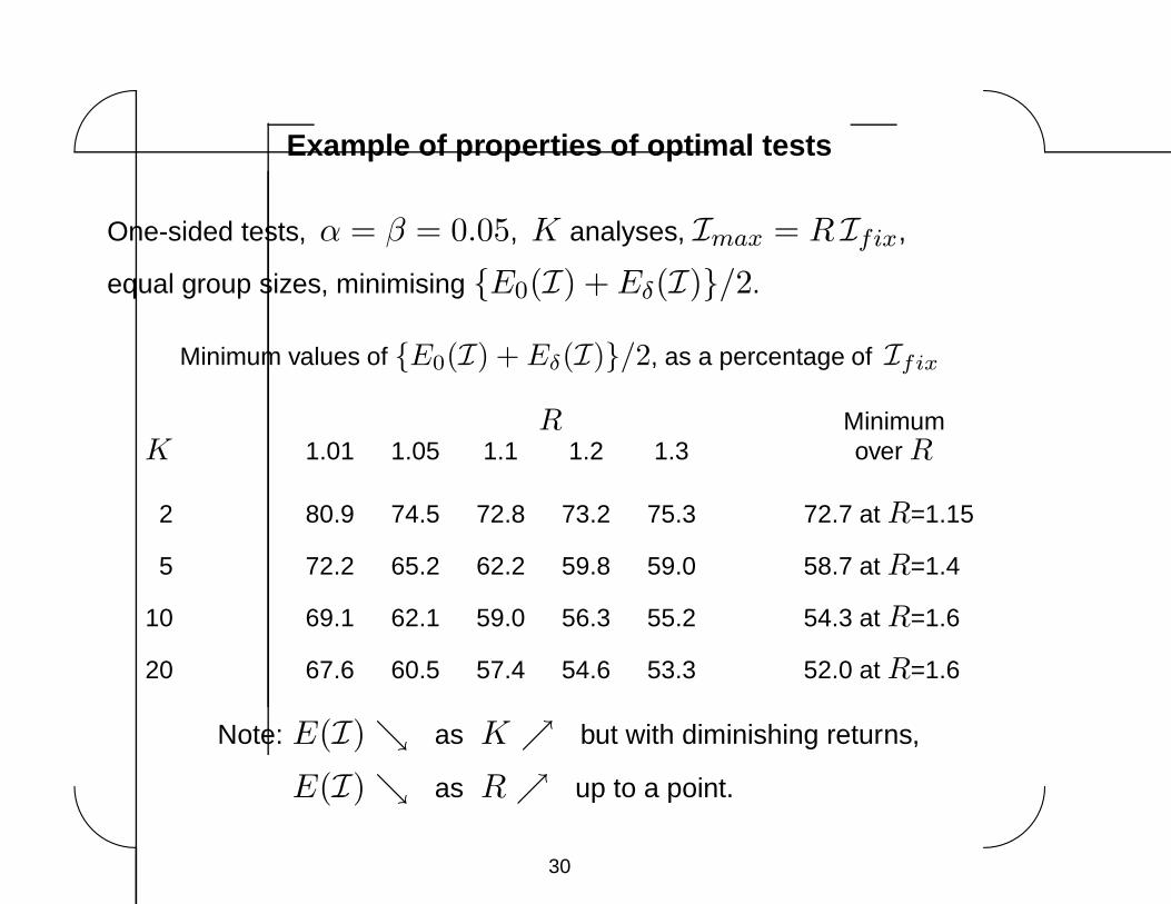
Example of properties of optimal tests

One-sided tests, α = β = 0.05, K analyses, Imax = R Ifix,

equal group sizes, minimising {E0(I) + Eδ(I)}/2.

Minimum values of {E0(I) + Eδ(I)}/2, as a percentage of Ifix

R MinimumK 1.01 1.05 1.1 1.2 1.3 over R

2 80.9 74.5 72.8 73.2 75.3 72.7 at R=1.15

5 72.2 65.2 62.2 59.8 59.0 58.7 at R=1.4

10 69.1 62.1 59.0 56.3 55.2 54.3 at R=1.6

20 67.6 60.5 57.4 54.6 53.3 52.0 at R=1.6

Note: E(I) ↘ as K ↗ but with diminishing returns,

E(I) ↘ as R ↗ up to a point.

30

'

&

$

%

Assessing families of group sequential tests

One-sided tests:

Pampallona & Tsiatis

Parametric family indexed by ∆, boundaries for Sk involve I ∆k ,

each ∆ implies an “inflation factor” R such that Imax = R Ifix.

Error spending, ρ-family

Error spent is proportional to I ρk , ρ determines the inflation factor R.

Error spending, γ-family (Hwang et al, 1994)

Error spent is proportional to

1 − e−γ Ik/Imax

1 − e−γ.

31

'

&

$

%

Families of tests

Tests with K = 10, α = 0.05, 1 − β = 0.9.

{E0(I) + Eδ(I)}/2 as a percentage of Ifix

1.0 1.1 1.2 1.3 1.4

6065

70

PSfrag replacements

optimal

� family

� family

� family

12

R

Both error spending families are highly efficient but Pampallona & Tsiatis

tests are sub-optimal.

Adapting optimally to observed data

32

'

&

$

%

Squeezing a little extra efficiency

Schmitz (1993) proposed group sequential tests in which group sizes are

chosen adaptively:

Initially, fix I1,

observe S1 ∼ N(θI1, I1 ),

then choose I2 as a function of S1, observe S2 where

S2 − S1 ∼ N( θ(I2 − I1), (I2 − I1) ),

and so forth.

Specify sampling rule and stopping rule to achieve desired overall type I

error rate and power.

33

'

&

$

%

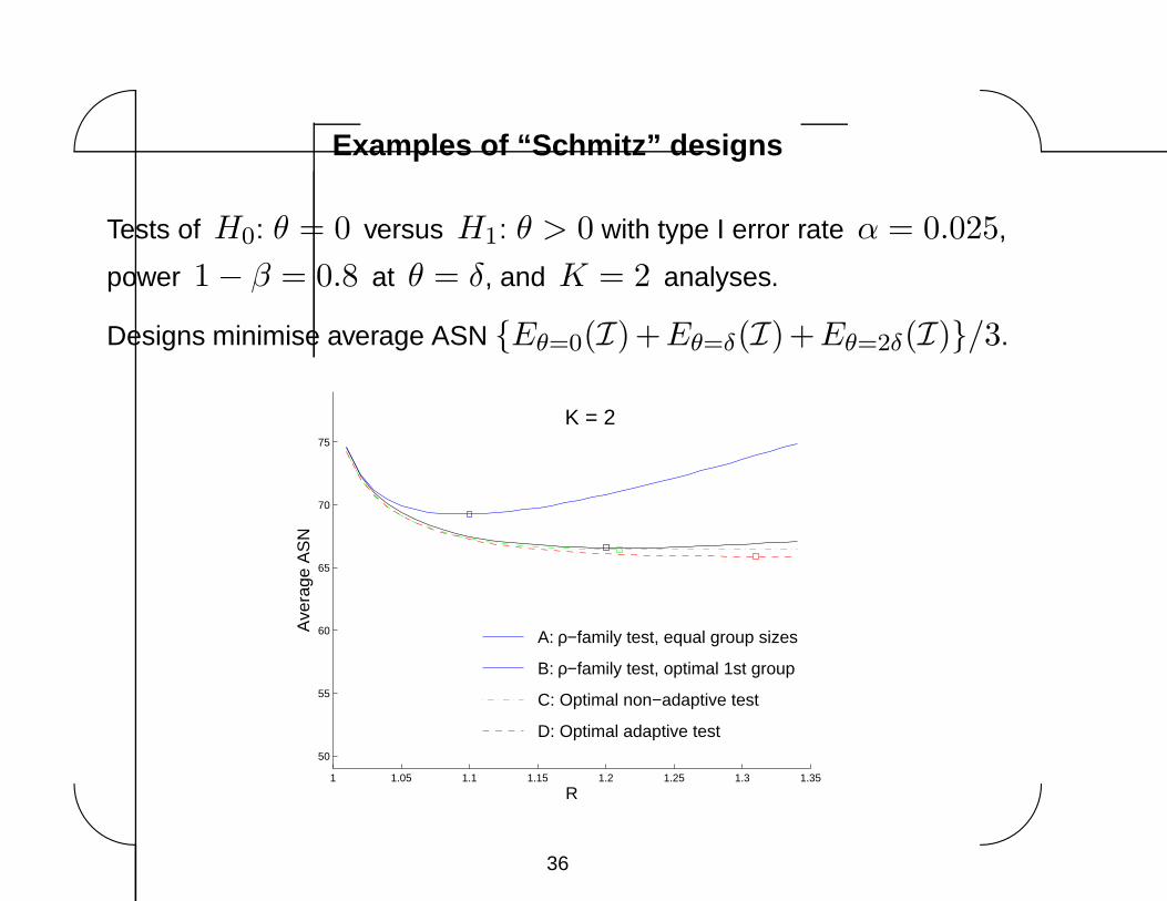
Examples of “Schmitz” designs

To test H0: θ = 0 versus H1: θ > 0 with type I error rate α = 0.025

and power 1 − β = 0.9 at θ = δ.

Aim for low values of ∫Eθ(N)f(θ) dθ,

where f(θ) is the density of a N(δ, δ2/4) distribution.

Constraints:

Maximum sample information = 1.2 × fixed sample information.

Maximum number of analyses = K .

Again, optimal designs can be found by solving related Bayes decision

problems.

34

'

&

$

%

Examples of “Schmitz” designs

Optimal average E(I) as a percentage of the fixed sample information.

Optimal Optimal Optimaladaptive non-adaptive, non-adaptive,

K design optimised equal group(Schmitz) group sizes sizes

2 72.5 73.2 74.8

3 64.8 65.6 66.1

4 61.2 62.4 62.7

6 58.0 59.4 59.8

8 56.6 58.0 58.3

10 55.9 57.2 57.5

Varying group sizes adaptively makes for a complex procedure and the

efficiency gains are slight.

Adapting super-optimally to observed data

35

'

&

$

%

Examples of “Schmitz” designs

Tests of H0: θ = 0 versus H1: θ > 0 with type I error rate α = 0.025,

power 1 − β = 0.8 at θ = δ, and K = 2 analyses.

Designs minimise average ASN {Eθ=0(I)+Eθ=δ(I)+Eθ=2δ(I)}/3.

1 1.05 1.1 1.15 1.2 1.25 1.3 1.35

50

55

60

65

70

75

R

Ave

rage

AS

N

A: ρ−family test, equal group sizes

B: ρ−family test, optimal 1st group

C: Optimal non−adaptive test

D: Optimal adaptive test

K = 2

36

'

&

$

%

Examples of “Schmitz” designs

Tests of H0: θ = 0 versus H1: θ > 0 with type I error rate α = 0.025,

power 1 − β = 0.8 at θ = δ, and K = 5 analyses.

Designs minimise average ASN {Eθ=0(I)+Eθ=δ(I)+Eθ=2δ(I)}/3.

1 1.2 1.4 1.6 1.8 2

30

35

40

45

50

55

60

65

R

Ave

rage

AS

N

A: ρ−family test, equal group sizes

B: ρ−family test, optimal 1st group

C: Optimal non−adaptive test

D: Optimal adaptive test

K = 5

37

'

&

$

%

5. Recent adaptive methods

“Adaptivity” 6= “Flexibility”

• Pre-planned extensions. The way the design changes in response to

interim data is pre-determined: Proschan and Hunsberger (1995), Li et

al. (2002), Hartung and Knapp (2003) — very much like “Schmitz”

designs.

• Partially pre-planned. The time of the first interim analysis is

pre-specified, as is the method for combining results from different

stages: Bauer (1989), Bauer & Kohne (1994).

• Re-design may be unplanned. The method of combining results from

different stages is implicit in the original design and carried over into

any re-design: Fisher (1998), Cui et al. (1999), Denne (2001) or Muller

& Schafer (2001).

38

'

&

$

%

Bauer (1989) and Bauer & Kohne (1994) . . .

. . . proposed mid-course design changes to one or more of

Treatment definition

Choice of primary response variable

Sample size:

— in order to maintain power under an

estimated nuisance parameter

— to change power in response to external

information

— to change power for internal reasons

a) secondary endpoint, e.g., safety

b) primary endpoint, i.e., θ.

39

'

&

$

%

Bauer & Kohne’s two-stage scheme

Investigators decide at the design stage to split the trial into two parts.

Each part yields a one-sided P-value and these are combined.

• Run part 1 as planned. This gives

P1 ∼ U(0, 1) under H0.

• Make design changes.

• Run part 2 with these changes, giving

P2 ∼ U(0, 1) under H0,

conditionally on P1 and other part 1 information.

• Combine P1 and P2 by Fisher’s combination test:

− log(P1 P2) ∼ 1

2χ2

4 under H0.

40

'

&

$

%

B & K: Major design changes before part 2

With major changes, the two parts are rather like separate studies in a

drug development process, such as:

Phase IIbCompare several doses and select the best.

Use a rapidly available endpoint (e.g., tumour response).

Phase IIICompare selected dose against control.

Use a long-term endpoint (e.g., survival).

Applying Fisher’s combination test for P1 and P2 gives a meta-analysis of

the two stages with a pre-specified rule.

Note: Each stage has its own null hypothesis and the overall H0 is the

intersection of these.

41

'

&

$

%

B & K: Minor design changes before stage 2

With only minor changes, the form of responses in stage 2 stays close to

the original plan.

Bauer & Kohne’s method provides a way to handle this.

Or, an error spending test could be used:

Slight departures from the original design will perturb the observed

information levels, which can be handled in an error spending design.

After a change of treatment definition, one can stratify with respect to

patients admitted before and after the change. As long as the overall score

statistic can be embedded in a Brownian motion, one can use an error

spending test with a maximum information design.

42

'

&

$

%

B & K: Nuisance parameters

Example. Normal response with unknown variance, σ2.

Aiming for type I error rate α and power 1 − β at θ = δ, the necessary

sample size depends on σ2.

One can choose the second stage’s sample size to meet this power

requirement assuming variance is equal to s21, the estimate from stage 1.

P1 and P2 from t-tests are independent U(0, 1) under H0 — exactly.

Other methods:

(a) Many “internal pilot” designs are available.

(b) Error spending designs can use estimated information (from s2).

(c) The two-stage design of Stein (1945) attains both type I error and

power precisely!

43

'

&

$

%

External factors or internal, secondary information

At an interim stage suppose, for reasons not concerning the primary

endpoint, investigators wish to achieve power 1 − β at θ = δ rather

than θ = δ (δ < δ).

If this happens after part 1 of a B & K design, the part 2 sample size can

be increased, e.g., to give conditional power 1 − β at θ = δ.

Unplanned re-design

Recent work shows the same can be done within a fixed sample or group

sequential design by

preserving conditional type I error rate under θ = 0,

ensuring conditional power 1 − β at θ = δ

— see Denne (2001) or Muller & Schafer (2001).

44

'

&

$

%

Responding to θ, an estimate of the primary endpoint

Motivation may be:

• to rescue an under-powered study,

• a “wait and see” approach to choosing a study’s power requirement,

• trying to be efficient.

Many methods have been proposed to do this.

If re-design is unplanned, the conditional type I error rate approach is

available.

It is good to be able to rescue a poorly designed study.

But, group sequential tests already base the decision for early

stopping on θ — and optimal GSTs do this optimally!

45

'

&

$

%

The variance spending method

L. Fisher (1998), Cui et al. (1999), Denne (2001), . . .

As before, consider study with two parts.

B & K used R.A. Fisher’s inverse χ2 method to combine P1, P2.

Instead we use the weighted inverse normal method (Mosteller and Bush

1954):

Define Z1 = Φ−1(1 − P1) Z2 = Φ−1(1 − P2)

Note Z2 ∼ N(0, 1) under H0 conditionally on P1, Z1 and other part 1

information.

Suppose w1, w2 are fixed weights with w21 + w2

2 = 1.

Then Z = w1Z1 + w2Z2 ∼ N(0, 1) and test that rejects H0 when

Z > z(α) has level α.

46

'

&

$

%

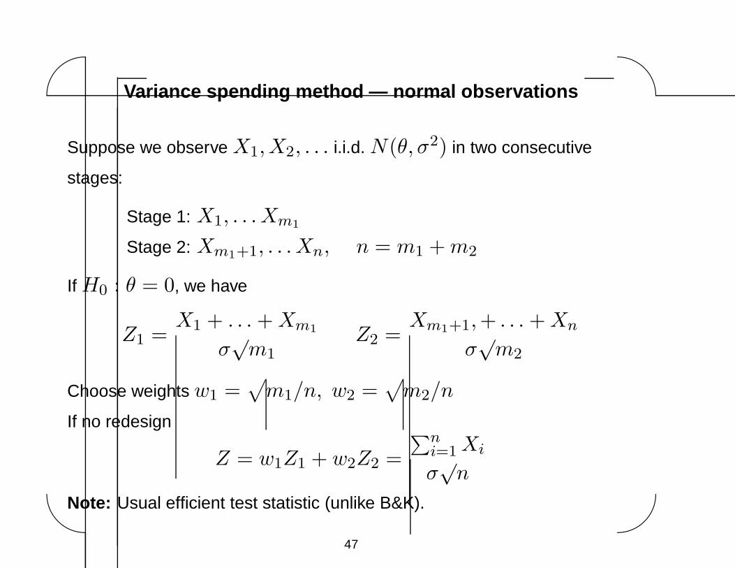
Variance spending method — normal observations

Suppose we observe X1,X2, . . . i.i.d. N(θ, σ2) in two consecutive

stages:

Stage 1: X1, . . . Xm1

Stage 2: Xm1+1, . . . Xn, n = m1 + m2

If H0 : θ = 0, we have

Z1 =X1 + . . . + Xm1

σ√

m1

Z2 =Xm1+1,+ . . . + Xn

σ√

m2

Choose weights w1 =√

m1/n, w2 =√

m2/n

If no redesign

Z = w1Z1 + w2Z2 =

∑ni=1 Xi

σ√

n

Note: Usual efficient test statistic (unlike B&K).

47

'

&

$

%

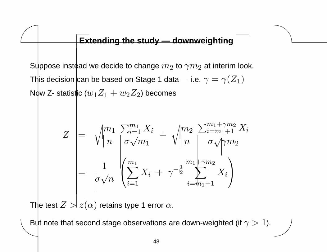
Extending the study — downweighting

Suppose instead we decide to change m2 to γm2 at interim look.

This decision can be based on Stage 1 data — i.e. γ = γ(Z1)

Now Z- statistic (w1Z1 + w2Z2) becomes

Z =

√m1

n

∑m1

i=1 Xi

σ√

m1

+

√m2

n

∑m1+γm2

i=m1+1 Xi

σ√

γm2

=1

σ√

n

m1∑

i=1

Xi + γ−1

2

m1+γm2∑

i=m1+1

Xi

The test Z > z(α) retains type 1 error α.

But note that second stage observations are down-weighted (if γ > 1).

48

'

&

$

%

6. Example of inefficiency in an adaptive design

Example. A Cui, Hung & Wang (1999) style example.

Scenario.

We wish to design a test with type I error probability α = 0.025.

Investigators are optimistic the effect, θ, could be as high as δ∗ = 20.

However, effect sizes as low as about θ ≥ δ∗∗ = 15 are clinically relevant

and worth detecting (cf the example cited by Cui et al).

First, consider a fixed sample study attaining power 0.9 at θ = δ∗ = 20.

We suppose this requires a sample size nf = 100.

An adaptive design starts out as a fixed sample test with nf = 100

observations, but the data are examined after the first 50 responses to see

if there is a need to “adapt”.

49

'

&

$

%

Cui et al. adaptive design

Denote the estimated effect based on the first 50 observations by θ1.

If θ1 < 0.2 δ∗ = 4, stop the trial for futility, accepting H0.

Otherwise, re-design the remainder of the trial, preserving the conditional

type I error rate given θ1 — thereby maintaining overall type I error rate

α.

Choose the remaining sample size to give conditional power 0.9 if in fact

θ = θ1.

Then, truncate this additional sample size to the interval (50, 500), so no

decrease in sample size is allowed and we keep the total sample size to at

most 550.

50

'

&

$

%

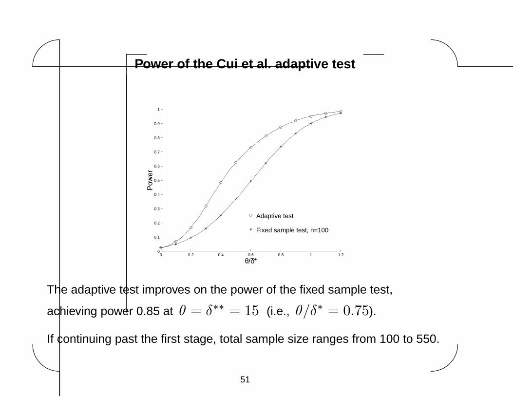
Power of the Cui et al. adaptive test

0 0.2 0.4 0.6 0.8 1 1.20

0.1

0.2

0.3

0.4

0.5

0.6

0.7

0.8

0.9

1

θ/δ*

Pow

er

Fixed sample test, n=100

Adaptive test

The adaptive test improves on the power of the fixed sample test,

achieving power 0.85 at θ = δ∗∗ = 15 (i.e., θ/δ∗ = 0.75).

If continuing past the first stage, total sample size ranges from 100 to 550.

51

'

&

$

%

A conventional group sequential test

Similar overall power can be obtained by a non-adaptive GST designed to

attain power 0.9 when θ = 14.

We have compared a power family, error spending test with ρ = 1:

type I error rate is α = 0.025,

taking the first analysis after 68 observations and the second analysis

after 225 gives a test meeting the requirement of power 0.9 at θ = 14.

This test dominates the Cui et al. adaptive design with respect to both

power and ASN. It also has a much lower maximum sample size — 225

compared to 550.

52

'

&

$

%

Cui et al. adaptive test vs non-adaptive GST

0 0.2 0.4 0.6 0.8 1 1.20

0.1

0.2

0.3

0.4

0.5

0.6

0.7

0.8

0.9

1

θ/δ*

Pow

er

Adaptive test

2−group GST

0 0.2 0.4 0.6 0.8 1 1.20

50

100

150

200

θ/δ*

AS

N

Adaptive test

2−group GST

The advantages of the conventional GST are clear. It has higher power, a

lower average sample size function, and a much smaller maximum sample

size.

We have found similar inefficiency in many more of the adaptive designs

proposed in the literature.

53

'

&

$

%

Conditional power and overall power

It might be argued that only conditional power is important once a study is

underway so overall power is irrelevant once data have been observed.

However:

Overall power integrates over conditional properties in just the right way.

It is overall power that is available at the design stage, when a stopping

rule and sampling rule (even an adaptive one) are chosen.

As the example shows, “chasing conditional power” can be a trap leading

to very large sample sizes when the estimated effect size is low — and,

given the variability of this estimate, the true effect size could well be zero.

To a pharmaceutical company conducting many trials, long term

performance is determined by overall properties, i.e., the power and

average sample size of each study.

54

'

&

$

%

7. Conclusions

Error Spending tests using Information Monitoring can adapt to

• unpredictable information levels,

• nuisance parameters,

• observed data, i.e., efficient stopping rules.

Methods preserving conditional type I error allow re-design in response

to external developments or internal evidence from secondary endpoints.

Recently proposed adaptive methods can

facilitate re-sizing for nuisance parameters,

support re-sizing to rescue an under-powered study,

allow an on-going approach to study design.

But, they will not improve on the efficiency of “standard” Group Sequential

Tests — and they can be substantially inferior.

55

'

&

$

%

References

Bauer, P. (1989). Multistage testing with adaptive designs (with discussion). Biometrie und Informatik in Medizin und Biologie 20,

130–148.

Bauer, P. and Kohne, K. (1994). Evaluation of experiments with adaptive interim analyses. Biometrics 50, 1029–1041. Correction

Biometrics 52, (1996), 380.

Chi, G.Y.H. and Liu, Q. (1999). The attractiveness of the concept of a prospectively designed two-stage clinical trial. J.

Biopharmaceutical Statistics 9, 537–547.

Cui, L., Hung, H.M.J. and Wang, S-J. (1999). Modification of sample size in group sequential clinical trials. Biometrics 55, 853–857.

Denne, J.S. (2001). Sample size recalculation using conditional power. Statistics in Medicine 20, 2645–2660.

ICH Topic E9. Note for Guidance on Statistical Principles for Clinical Trials. ICH Technical Coordination, EMEA: London, 1998.

Fisher, L.D. (1998). Self-designing clinical trials. Statistics in Medicine 17, 1551–1562.

Fisher, R.A. (1932). Statistical Methods for Research Workers, 4th Ed., Oliver and Boyd, London.

Hartung, J. and Knapp, G. (2003). A new class of completely self-designing clinical trials. Biometrical Journal 45, 3-19.

Hwang, I.K., Shih, W.J. and DeCani, J.S. (1990). Group sequential designs using a family of type I error probability spending functions.

Statist. Med., 9, 1439–1445.

Jennison, C. and Turnbull, B.W. (1993). Group sequential tests for bivariate response: Interim analyses of clinical trials with both

efficacy and safety endpoints. Biometrics 49, 741–752.

Jennison, C. and Turnbull, B.W. (2000). Group Sequential Methods with Applications to Clinical Trials, Chapman & Hall/CRC, Boca

Raton.

Jennison, C. and Turnbull, B.W. (2003). Mid-course sample size modification in clinical trials based on the observed treatment effect.

Statistics in Medicine 23, 971–993.

56

'

&

$

%

Jennison, C. and Turnbull, B.W. (2004a,b,c). Preprints available at http://www.bath.ac.uk/˜mascj/ or at

http://www.orie.cornell.edu (Click on “Technical Reports”, “Faculty Authors”, “Turnbull” and finally on “Submit”).

a. Efficient group sequential designs when there are several effect sizes under consideration.

b. Adaptive and non-adaptive group sequential tests.

c. Meta-analyses and adaptive group sequential designs in the clinical development process.

Li, G., Shih, W. J., Xie, T. and Lu. J. (2002). A sample size adjustment procedure for clinical trials based on conditional power.

Biostatistics 3, 277–287.

Mehta, C. R. and Tsiatis, A. A. (2001). Flexible sample size considerations using information-based interim monitoring. Drug

Information J. 35, 1095–1112.

Muller, H-H. and Schafer, H. (2001). Adaptive group sequential designs for clinical trials: Combining the advantages of adaptive and of

classical group sequential procedures. Biometrics 57, 886–891.

Pampallona, S. and Tsiatis, A.A. (1994). Group sequential designs for one-sided and two-sided hypothesis testing with provision for

early stopping in favor of the null hypothesis. J. Statist. Planning and Inference, 42, 19–35.

Pocock, S.J. (1977). Group sequential methods in the design and analysis of clinical trials. Biometrika, 64, 191–199.

Proschan, M.A. and Hunsberger, S.A. (1995). Designed extension of studies based on conditional power. Biometrics 51, 1315–1324.

Schmitz, N. (1993). Optimal Sequentially Planned Decision Procedures. Lecture Notes in Statistics, 79, Springer-Verlag: New York.

57