Adaptively Varying Coefficient Spatio-Temporal...
28
Adaptively Varying Coefficient Spatio-Temporal Models ∗ Zudi Lu 1,2,3 Dag Johan Steinskog 4,5 Dag Tjøstheim 6 Qiwei Yao 1,7 1 Department of Statistics, London School of Economics, London, WC2A 2AE, UK 2 Department of Mathematics & Statistics, Curtin University of Technology, Perth, Australia 3 School of Mathematical Sciences, The University of Adelaide, Adelaide, Australia 4 Nansen Environmental and Remote Sensing Center, 5006 Bergen, Norway 5 Bjerknes Centre for Climate Research, 5007 Bergen, Norway 6 Department of Mathematics, University of Bergen, 5007 Bergen, Norway 7 Guanghua School of Management, Peking University, Beijing 100871, China Abstract We propose an adaptive varying-coefficient spatio-temporal model for data observed irreg- ularly over space and regularly in time. The model is capable of catching possible nonlinearity (both in space and in time) and nonstationarity (in space) by allowing the autoregressive co- efficients to vary with both spatial location and an unknown index variable. We suggest a two-step procedure to estimate both the coefficient functions and the index variable, which is readily implemented and can be computed even for large spatio-temporal data sets. Our theoretical results indicate that in the presence of the so-called nugget effect, the errors in the estimation may be reduced via the spatial smoothing – the second step in the proposed estimation procedure. The simulation results reinforce this finding. As an illustration, we apply the methodology to a data set of sea level pressure in the North Sea. Key words: β -mixing, kernel smoothing, local linear regression, nugget effect, spatial smoothing, unilateral order. ∗ Partially supported by a Leverhulme Trust research grant and EPSRC research grant. Lu’s work was also partially supported by an Internal Research Grant from Curtin University of Technology and the Discovery Grant from Australian Research Council. 1
Transcript of Adaptively Varying Coefficient Spatio-Temporal...

Adaptively Varying Coefficient Spatio-Temporal Models∗
Zudi Lu1,2,3 Dag Johan Steinskog4,5 Dag Tjøstheim6 Qiwei Yao1,7
1Department of Statistics, London School of Economics, London, WC2A 2AE, UK
2Department of Mathematics & Statistics, Curtin University of Technology, Perth, Australia
3 School of Mathematical Sciences, The University of Adelaide, Adelaide, Australia
4 Nansen Environmental and Remote Sensing Center, 5006 Bergen, Norway
5Bjerknes Centre for Climate Research, 5007 Bergen, Norway
6Department of Mathematics, University of Bergen, 5007 Bergen, Norway
7Guanghua School of Management, Peking University, Beijing 100871, China
Abstract
We propose an adaptive varying-coefficient spatio-temporal model for data observed irreg-
ularly over space and regularly in time. The model is capable of catching possible nonlinearity
(both in space and in time) and nonstationarity (in space) by allowing the autoregressive co-
efficients to vary with both spatial location and an unknown index variable. We suggest a
two-step procedure to estimate both the coefficient functions and the index variable, which
is readily implemented and can be computed even for large spatio-temporal data sets. Our
theoretical results indicate that in the presence of the so-called nugget effect, the errors in
the estimation may be reduced via the spatial smoothing – the second step in the proposed
estimation procedure. The simulation results reinforce this finding. As an illustration, we
apply the methodology to a data set of sea level pressure in the North Sea.
Key words: β-mixing, kernel smoothing, local linear regression, nugget effect, spatial smoothing,
unilateral order.
∗Partially supported by a Leverhulme Trust research grant and EPSRC research grant. Lu’s work was also
partially supported by an Internal Research Grant from Curtin University of Technology and the Discovery Grant
from Australian Research Council.
1

1 Introduction
The wide availability of data observed over time and space, in particular through inexpensive
geographical information systems, has stimulated many studies in a variety of disciplines such as
environmental science, epidemiology, political science, demography, economics and geography. In
these studies, the geographical areas (e.g. counties, census tracts) are taken as units of analysis,
and specific statistical methods have been developed to deal with the spatial structure reflected in
the distribution of the dependent variable; see e.g. Ripley (1981), Anselin (1988), Cressie (1993),
Guyon (1995), Stein (1999) and Diggle (2003) for systematic reviews of these and related topics.
In this paper we are concerned with spatio-temporal data which are measured or transformed
to a continuous scale and observed irregularly over space but regularly over time. Data sets of this
form exist extensively. It may be environmental monitoring stations located irregularly in some
region, but with measurements taken daily; see for instance Fotheringham et al. (1998), Brunsdon
et al. (2001), Fuentes (2001), Zhang et al. (2003). Applications in spatial disease modelling may
be found in Knorr-Held (2000), Lagazio et al. (2001).
Our model is of the form
Yt(s) = a {s, α(s)τXt(s)} + b1{s, α(s)τXt(s)}τXt(s) + εt(s), (1.1)
where Yt(s) is the spatio-temporal variable of interest, and t is time, s = (u, v) ∈ S ⊂ R2 is a
spatial location. Moreover, a(s, z) and b1(s, z) are unknown scalar and d×1 functions, α(s) is an
unknown d× 1 index vector, {εt(s)} is a noise process which, for each fixed s, forms a sequence of
i.i.d. random variables over time, and Xt(s) = {Xt1(s), · · · , Xtd(s)}τ consists of time-lagged values
of Yt(·) in a neighbourhood of s and, possibly, some exogenous variables. Throughout the paper
we use τ to denote the transpose of a vector or a matrix. We let both the regression coefficient b1
and the intercept a depend on the location s, as well as on the index variable α(s)τXt(s), to catch
possible nonstationary features over space. Model (1.1) is unilateral in time and, therefore, it can
be easily simulated in a Monte Carlo study. Furthermore it is readily applicable to model practical
problems. Those features make the model radically different from purely spatial autoregressive
models (Yao and Brockwell 2006). Also note that at a given location s, the coefficient functions
are univariate functions of α(s)τXt(s). Therefore only one-dimensional smoothing is required in
estimating those coefficients. (See Section 2.2.1 below).
Model (1.1) is proposed to model nonlinear and nonstationary spatial data in a flexible manner.
Note that the literature on spatial processes is overwhelmingly dominated by linear models. On
1

the other hand, many practical data exhibit clearly nonlinear and nonstationary features. For
example, in our analysis of the daily mean sea level pressure (MSLP) readings in Section 5, the
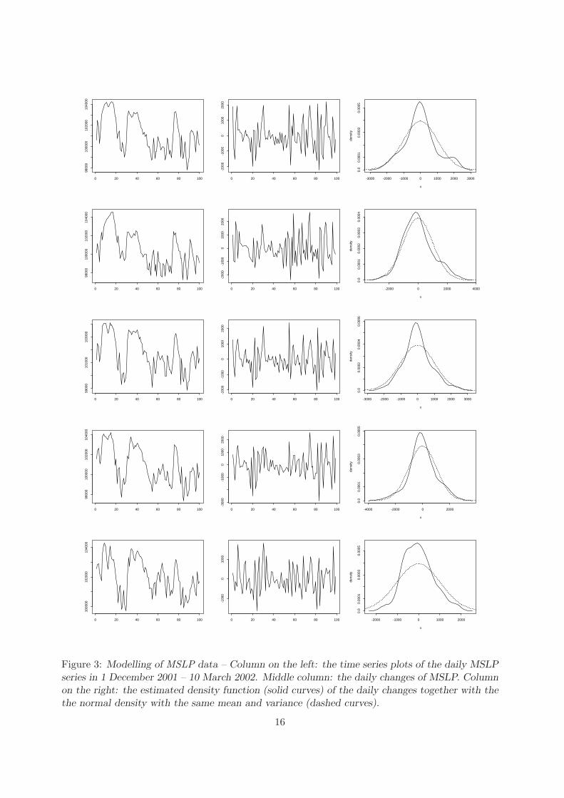
original time series at each location is non-linear. Figure 3 below displays the plots for the MSLP
data at five randomly selected locations. There are roughly three high pressure periods within
the time span concerned. In the middle column of Figure 3, the correlation structure of the
differenced series in the high pressure periods is different from that of the low pressure periods
and the transition periods. This naturally calls for a nonlinear model with varying coefficients
depending also on the past values of the variables from the neighbourhood locations. Such a
dynamics cannot result in a Gaussian marginal distribution, as indicated in the plots on the right
column in Figure 3. The estimated densities are more peaked than the normal distribution, the
accumulation of density mass around zero being due to the high pressure activity.
Model (1.1) is a spatial extension of the adaptive varying-coefficient linear model of Fan
et al. (2003), see also Xia and Li (1999). Due to the spatial non-stationarity of the model, we adopt
an estimation strategy involving two steps, which also facilitates the parallel computation over
different locations. First, for each fixed location s, we estimate the varying coefficient functions
a and b1 and the index vector α based on the observations at the location s only. This is a
time series estimation problem. Our estimation is based on local linear regression. The second
step is to apply spatial smoothing to pool together the information from neighbourhood locations.
Asymptotic properties of our estimators have been established, which indicate that in the presence
of the so-called ‘nugget effect’, the spatial smoothing will reduce the estimation errors. (See also
Lu et al. 2008). Our simulation study reinforces this finding.
As far as we are aware, this is the first paper to address spatio-temporal nonlinear dependence
structures with spatial nonstationarity and non-Gaussian distributions. Earlier work on nonlinear
and/or non-Gaussian spatial models includes, among others, Matheron (1976), Rivoirard (1994),
Chiles and Delfiner (1999, Chapter 6), Hallin et al. (2004a, 2004b), Biau and Cadre (2004), Gao
et al. (2006), Lu et al. (2007).
The structure of the paper is as follows. We introduce our methodology in Section 2. Illus-
tration with simulated examples are reported in Section 3. In Section 5 there is an application
to a data set of sea level pressure in the North Sea, for which the index variable may be viewed
as an analogue of a spatial principal component used in the so-called EOF analysis for climate
time series. The asymptotic properties are reported in Section 4, with the regularity conditions
deferred to an appendix.
2

2 Methodology
2.1 Identification
Model (1.1) is not identifiable. In fact, it may be equivalently expressed as
Yt(s) = [a{s, α(s)τXt(s)} + κ{s, α(s)τXt(s)}α(s)τXt(s)]
+ [b1{s, α(s)τXt(s)} − κ{s, α(s)τXt(s)}α(s)]τ Xt(s) + εt(s), (2.1)
for any real-valued function κ(·). To overcome this problem, we may assume that the last com-
ponent of α(s) is non-zero, the first non-zero component of α(s) is positive, and ||α(s)||2 = 1.
Based on those assumptions, Fan et al. (2003) impose the condition that the last component of
b1 is 0 in (1.1). Put b1 = (bτ , 0)τ . This effectively reduces (1.1) to the form
Yt(s) = a{s, α(s)τXt(s)} + [b{s, α(s)τXt(s)}]τ Xt(s) + εt(s), (2.2)
where Xt(s) = {Xt,1(s) · · · , Xt,d−1(s)}τ . In fact, α, a and b in (2.2) are now identifiable as
long as the regression function E{Yt(s)|Xt(s) = x} is not of the form ατxβτx + γτx + c, where
β, γ ∈ Rd, c ∈ R
1 are constants only related to s; see Theorem 1(b) of Fan et al. (2003). Note
that (2.1) reduces to (2.2) by setting κ(s, z) = b1d/αd, where b1j and αj denote, respectively, the
j-th component of b1(s, z) and α(s).
A disadvantage of the form (2.2) is that all the components of Xt(s) are not on an equal footing,
which may cause difficulties in model interpretation. This may be particularly problematic when
Xt(s) consists of neighbour variables of Yt(s). One possible remedy is to impose an orthogonal
constraint in the model instead, that is
Yt(s) = a⋆{s, α(s)τXt(s)} + b1{s, α(s)τXt(s)}τXt(s) + εt(s), α(s)τb1(s, z) = 0. (2.3)
In fact such an orthogonal representation may be obtained from (2.2) with
a⋆(s, z) = a(s, z) + α(s)(b(s, z)τ , 0)z and b1(s, z) = (b(s, z)τ , 0)τ − α(s)(b(s, z)τ , 0)α(s) (2.4)
while α(s) remains unchanged. Note the condition α(s)τb1(s, z) = 0 is fulfilled as ||α(s)||2 = 1.
Furthermore, (2.3) is an equivalent representation of (2.2), and it is identifiable as long as (2.2)
is identifiable. To see this, we first note that (2.2) may be deduced from (2.3) by letting
a(s, z) = a⋆(s, z) +b1d
αdz and b(s, z) = (b11, · · · , b1,d−1)
τ −b1d
αd(α1, · · · , αd−1)
τ . (2.5)
3

This is effectively to write the first equation in (2.3) in the form of (2.1) with (a, κ) replaced by
(a⋆, b1d/αd). Moreover, as α(s)τb1(s, z) = 0 and ||α(s)||2 = 1, it follows from the second equality
in (2.5) that
(b(s, z)τ , 0)α(s) =d−1∑
j=1
αjb1j −b1d
αd
d−1∑
j=1
α2j = −αdb1d −
b1d
αd(1 − α2
d) = −b1d
αd.
Hence the d-component b1d of b1(s, z) is identifiable when model (2.2) is identifiable. This,
together with (2.5), implies that all the other components of b1(s, z) as well as a⋆(s, z) are also
identifiable.
Since the orthogonal constraint ατb1 = 0 in (2.3) poses further technical complication in
inference, in the sequel we proceed with the identifiable model (2.2), assuming that the first non-
zero element of α(s) is positive. Only for the real data example in section 5, we present the fitted
model in the form (2.3) via the transformation (2.4).
2.2 Estimation
With the observations {Yt(si), Xt(si)} for t = 1, · · · , T and i = 1, · · · , N , we estimate a,b and
α in model (2.2) in two steps: (i) For each fixed s = si, we estimate them using the time series
data {Yt(s),Xt(s), t = 1, · · · , T} only. (ii) By pooling the information from neighbour locations
via spatial smoothing, we improve the estimators obtained in (i). The second step also facilitates
the estimation at a location s with no direct observations (i.e. s 6= si for 1 ≤ i ≤ N).
2.2.1 Time Series Estimation
For a fixed s, we estimate the direction α(s) and the coefficient functions a(s, ·) and b(s, ·). Fan
et al. (2003) proposed a backfitting algorithm to solve this estimation problem. We argue that
with modern computer power, the problem can be dealt with in a more direct manner even for
moderately large d such as d between 10 and 20. Note that once the direction α(s) is fixed, the
estimators for a and b may be obtained by one-dimensional smoothing over α(s)τXt(s) using, for
example, the standard kernel regression methods.
We consider the estimation for α(s) first. If the coefficient functions a and b were known, we
may estimate α by solving a nonlinear least squares problem; see (2.7) below. Since a and b are
unknown, we may plug in their appropriate estimators instead. By doing so, we will have used
the same observations twice. Note that those estimators themselves are functions of α. Hence a
cross-validation approach will be employed to mitigate the effect of the double use of the same
4

data set. For any α(s), define the leave-one-out estimators a−t(s, z) = a and b−t(s, z) = b, where
(a, b) minimises
1
T − 1
∑
1≤j≤T
j 6=t
{Yj(s) − a − bτ Xj(s)
}2Kh{α
τ (s)Xj(s) − z}, (2.6)
where Kh(·) = h−1K(·/h), K(·) is a kernel function and h > 0 is a bandwidth. Then we choose
α(s) and h which minimise
R(α, h) =1
T
T∑
t=1
[Yt(s) − a−t{s, α
τXt(s)} − b−t{s, ατXt(s)}
τ Xt(s)]2
w{ατXt(s)}, (2.7)
where w(·) is a weight function which controls the boundary effect. In the above definition for the
estimator α(s), we used the Nadaraya-Watson estimators a and b in (2.6) to keep the function
R(α, h) simple. The asymptotic property of the estimator α(s) has been derived based on the
results of Lu et al. (2007); see (4.11) in section 4 below. The minimisation of R(·) may be carried
out using, for example, the downhill simplex method (section 10.4 of Press et al. 1992).
Once α(s) = α(s) is known, we may estimate a and b using univariate local linear regression
estimation. To this end, let (a, b, c, d) be the minimisers of
1
T
T∑
j=1
[Yj(s) − a − c(Zj − z) − {b − d(Zj − z)}τXj(s)
]2Kh(Zj − z), (2.8)
where Zt = α(s)τXt(s), and a different bandwidth h from the h in (2.6) will be used. Note that
both h and h are depending on T . The estimators for the functions a(s, ·) and b(s, ·) at z are
defined as a(s, z) = a and b(s, z) = b.
2.2.2 Spatial smoothing
Although we do not assume stationarity over space, improvement in estimation of a,b and α over
s may be gained by extracting information from neighbourhood locations, due to the continuity
of the functions concerned. Zhang et al. (2003) showed for the model they considered that it
was indeed the case in the presence of the nugget effect (Cressie, 1993, § 2.3.1). See also Lu
et al. (2008). Furthermore, the spatial smoothing provides a way to extrapolate our estimators
to the locations at which observations are not available.
Let W (·) be a kernel function defined on R2. Put Wh(s) = h−2W (s/h), where h > 0 is a
bandwidth depending on the size N of spatial samples. The bandwidth h is different from both
5

h and h in the last subsection. Based on the estimators obtained above for each of the locations
s1, · · · , sN , the spatially smoothed estimators at the location s0 are defined as
α(s0) =N∑
j=1
α(sj)Wh(sj − s0)/ N∑
j=1
Wh(sj − s0), (2.9)
a(s0, z) =N∑
j=1
a(sj , z)Wh(sj − s0)/ N∑
j=1
Wh(sj − s0), (2.10)
b(s0, z) =N∑
j=1
b(sj , z)Wh(sj − s0)/ N∑
j=1
Wh(sj − s0). (2.11)
2.3 Bandwidth selection
Fan et al. (2003) outlined an empirical rule for selecting a bandwidth in fitting non-spatial varying-
coefficient regression models. Below we adapt that idea to determining bandwidths h in (2.8) and
h in (2.9) – (2.11). Note that the bandwidth h in (2.7) is selected, together with α(s), by cross-
validation.
We first deal with the selection of h in (2.8). Let
CV1(h) =1
T
T∑
t=1
[Yt(s) − a−t,h{s, α
τXt(s)} − b−t,h{s, ατXt(s)}
τ Xt(s)]2
w{ατXt(s)}, (2.12)
where a−t,h{s, z} and b−t,h{s, z} are the leave-one-out estimators defined as in (2.8) but with the
term of j = t removed from the sum. Under appropriate regularity conditions (c.f. Lu, Tjøstheim
and Yao, 2007), it holds that
CV1(h) = c0 + c1h4 +
c2
T h+ oP (h4 + T−1h−1).
Thus, up to first order asymptotics, the optimal bandwidth is hopt = (c2/4Tc1)1/5. In practice,
the coefficients c0, c1 and c2 will be estimated from solving the least squares problem
minc0,c1,c2
q∑
k=1
{CV1k − c0 − c1h
4k − c2/(T hk)
}2, (2.13)
where CV1k = CV1(hk) obtained from (2.12), and h1, · · · , hq are q prescribed bandwidth values.
We let h = (c2/4T c1)1/5 when both c1 and c2 are positive. In the likely event that one of
them is nonpositive, we let h = arg min1≤k≤q CV1(hk). This bandwidth selection procedure is
computationally efficient as q is moderately small, i.e. we only need to compute q CV-values; see
Remark 2(c) in Fan et al. (2003). Furthermore the least squares estimation (2.13) also serves as
a smoother for the CV bandwidth estimates. Also see Ruppert (1997).
6

The bandwidth h in (2.9) – (2.11) may be determined in the same manner. For example, for
the estimator (2.9), the CV function is defined as
CV2(h) =1
N
N∑
i=1
[α(si) − α
−si,h(si)
]2,
which admits the asymptotic expansion
CV2(h) = d0 + d1h4 +
d2
Nh2+ oP (h4 + N−1h−2).
The resulting bandwidth is of the form h = {d2/(2Nd1)}1/6.
The CV bandwidth selection has been extensively studied in the literature. In the sense of
mean integrated squared error (MISE) the relative error of a CV-bandwidth is higher than that
of, for example, a plug-in method of Ruppert et al. (1995). However there is a growing body of
opinion (e.g., Mammem, 1990; Jones, 1991; Hardle & Vieu, 1992; and Loader, 1999) maintaining
that the selection of bandwidth should be targeted at estimating the unknown function instead
of the ideal bandwidth itself. Therefore, one should seek a bandwidth minimising the integrated
squared error (ISE) rather than the MISE, i.e., focusing on loss rather than risk. From this point
of view, the CV-bandwidth performs reasonably well (Hall and Johnstone, 1992, page 479). In
time series context, the argument for why cross-validation is an appropriate selection method for
the bandwidth can be found in Kim and Cox (1996), Quintela-del-Rıo (1996) and Xia and Li
(2002), among others.
3 A simulated example
Consider a spatio-temporal process
Yt+1(sij) = a{sij , Zt(sij)} + b1{sij , Zt(sij)}Yt(sij) + b2{sij , Zt(sij)}Xt(sij) + 0.1εt(sij)
defined on the grid points sij = (ui, vj), where
a(sij , z) = 3exp{ −2z2
1 + 7(ui + vj)
}, b1(sij , z) = 0.7 sin{7π(ui + vj)}, b2(sij , z) = 0.8z,
Zt(sij) =1
3{2Yt(sij) + 2Xt(sij) + Xt(si,j+1))}, Xt(sij) =
2
9
1∑
k=−1
1∑
ℓ=−1
et(si+k,j+ℓ),
and all εt(sij) and et(sij) are independent N(0, 1) random variables. Observations were taken
over N = 64 grid points {(ui, vj), 1 ≤ i, j ≤ 8}, where ui = vi = (i − 1)/8 with T = 60 or
7

100. For each given s = sij , we estimated the curves a(s, ·), b1(s, ·) and b2(s, ·) on the 11 grid
points zℓ = −0.5 + 0.1(ℓ − 1) (ℓ = 1, · · · , 11), as well as the index α(s) = (α1(s), α2(s), α3(s))τ ≡
(2/3, 2/3, 1/3)τ , which is independent of s. The accuracy of the estimation is measured by the
the squared estimation errors:
SEE{αj(s)} = {αj(s) − αj}2, j = 1, 2, 3,
SEE{a(s)} =1
11
11∑
ℓ=1
{a(s, zℓ) − a(s, zℓ)}2,
SEE{bk(s)} =1
11
11∑
ℓ=1
{bk(s, zℓ) − bk(s, zℓ)}2, k = 1, 2.
For each setting, we replicated the experiments 10 times. The SEE over the 64 grid points are
collectively displayed as boxplots in Figure 1 for T = 60, and in Figure 2 for T = 100 (i.e. each
of the boxplots is based on 10 × 64 = 640 SEE values). It is clear that the estimates defined in
section 2.2.1 are less accurate than those defined in section 2.2.2. In fact the gain from the spatial
smoothing is substantial. The plots also indicate that the estimation becomes more accurate when
T increases.
The improvement from the spatial smoothing is due to the fact that the functions to be es-
timated are continuous in s. If we view the observations {Yt(sij), Xt(sij)} as a sample from a
spatio-temporal process with s varying continuously over space, the sample paths of such an un-
derlying process are discontinuous over space, as both εt(s) and et(s) are independent at different
locations no matter how close they are. The spatial smoothing pulls together the information on
the mean function from neighbour locations. It is intuitively clear that there would not be any
gains from such a ‘local pulling’ if the sample realisations of both Xt(·) and εt(·) are continuous
in s. The improvement may be obtained when the observations pulled together bring in different
information, which is only possible when the sample realisations are discontinuous. The theory
developed in next section indicates that the spatial smoothing may indeed improve the estimation
when the ‘nugget effect’ is present, which results in the discontinuity in sample realisations as a
function of s. See also Lu et al. (2008) for more detailed discussions regarding the asymptotic
theory with or without nugget effect.
8

Panel A
0.0
0.05
0.10
0.15
0.20
0.25
0.30
Non-SS SS
squa
red
erro
r(a)
0.0
0.01
0.02
0.03
0.04
Non-SS SS
squa
red
erro
r
(b)
0.0
0.05
0.10
0.15
0.20
0.25
0.30
Non-SS SS
squa
red
erro
r
(c)
Panel B
01
23
45
Non-SS SS
squa
red
erro
r
(a)
010
2030
40
Non-SS SS
squa
red
erro
r
(b)
02
46
810
12
Non-SS SS
squa
red
erro
r
(c)
Figure 1: Simulation with T = 60 – Boxplots for the SEEs of the three components of α (PanelA), and the varying coefficient functions (Panel B): (a) a(·), (b) b1(·), (c) b2(·). The plots for theestimates defined in section 2.2.1 are labelled as ‘Non-SS’, and the plots for the spatial smoothingestimates are labelled as ‘SS’.
9

Panel A
0.0
0.05
0.10
0.15
0.20
0.25
0.30
Non-SS SS
squa
red
erro
r(a)
0.0
0.01
0.02
0.03
Non-SS SS
squa
red
erro
r
(b)
0.0
0.05
0.10
0.15
0.20
0.25
Non-SS SS
squa
red
erro
r
(c)
Panel B
01
23
4
Non-SS SS
squa
red
erro
r
(a)
010
2030
Non-SS SS
squa
red
erro
r
(b)
02
46
Non-SS SS
squa
red
erro
r
(c)
Figure 2: Simulation with T = 100 – Boxplots for the SEEs of the three components of α (PanelA), and the varying coefficient functions (Panel B): (a) a(·), (b) b1(·), (c) b2(·). The plots for theestimates defined in section 2.2.1 are labelled as ‘Non-SS’, and the plots for the spatial smoothingestimates are labelled as ‘SS’.
10

4 Asymptotic properties
The improvements due to the spatial smoothing have been illustrated via simulation in Section 3.
In this section, we derive the asymptotic bias and variance of the estimators (2.9) – (2.11), which
also show the benefits from spatial smoothing in the presence of the so-called nugget effect. Note
that those asymptotic approximations are derived without the stationarity over space. On the
other hand, the asymptotic normality for the time series estimators defined in Section 2.2.1 may
be derived from Theorems 3.1 and 3.2 of Lu et al. (2007). We introduce some notation first.
We always assume the true index α(s) ∈ B for all s ∈ S, where
B ={β = (β1, · · · , βd)τ ∈ R
d : ‖β‖ = 1, the first non-zero element is positive,
and the last element is non-zero with |βd| ≥ ǫ0}, (4.1)
and ǫ0 > 0 is a fixed constant. Put Xt(s) = (1, Xt(s)τ )τ = (1, Xt1(s), · · · , Xt,d−1(s))
τ , and
g(s, z, β) = [E{Xt(s)Xτt (s)|β
τXt(s) = z}]−1E{Xt(s)Yt(s)|βτXt(s) = z},
where the matrix inverse is ensured by Assumption C6 in the appendix. We denote the derivatives
of g as follows:
gz(s, z, β) = ∂g(s, z, β)/∂z, gβ(s, z, β) = ∂g(s, z, β)/∂βτ , gz(s, z, β) = ∂2g(s, z, β)/∂z2.
When β = α(s), we will often drop α(s) in g{s, z, α(s)} and its derivatives if no confusion arises.
It therefore follows from (2.2) that g{s, z}τ = g{s, z, α(s)}τ = {a(s, z),b(s, z)τ}. Further, we let
Zt(s) = α(s)τXt(s), and define
Γ(s) = E[g(s)τXt(s)Xt(s)
τ g(s)w{Zt(s)}], (4.2)
where g(s) = gz{s, Zt(s), α(s)}Xt(s)τ + gβ{s, Zt(s), α(s)}.
Let αj(s) and αj(s) be the j-th component of α(s) and its second order derivative matrix with
respect to s, respectively. Recall that h = hT and h = hT are the two bandwidths used for time
series smoothing in Section 2.2.1, and h = hN is the bandwidth for spatial smoothing in Section
2.2.2. Put µ2,K =∫
u2K(u) du, µ2,W =∫SuuτW (u)du and ν0,K =
∫K2(u) du, where K and W
are the two kernel functions used in our estimation.
Now we are ready to present the asymptotic biases and variances for the spatial smoothing
estimators α(s0), a(s0) and b(s0), which are derived when T → ∞. The key is to show that the
11

time series estimators α(s), a(s) and b(s) converge uniformly in s over a small neighbourhood of
s0, which is established using the results in Lu et al. (2007). Naturally the derived asymptotic
approximations for the biases and variances of α(s0), a(s0) and b(s0) depend on N , and those
approximations admit more explicit expressions when N → ∞. Note we write aN ≃ bN if
limN→∞ aN/bN = 1.
Theorem 4.1 Let conditions C1 – C10 listed in the Appendix hold. Assume that s0 ∈ S and
f(s0) > 0, where f(·) is given in condition C8. Then as T → ∞, it holds that
α(s0) − α(s0) = B1,N (s0)h2(1 + oP (1)) + B2,N (s0)
+ T−1/2 {V1,N (s0) + V2,N (s0)} η(s0)(1 + oP (1)),
where η(s0) is a d × 1 random vector with zero mean and identity covariance matrix,
B1,N (s) ≃ −1
2Γ−1(s)E[g(s)τ
Xt(s)Xt(s)τ gz{s, Zt(s), α(s)}w{Zt(s)}]µ2,K , (4.3)
B2,N (s) ≃1
2h2 (tr [α1(s)µ2,W ] , · · · , tr [αd(s)µ2,W ])τ , (4.4)
and V1,N (s0) and V2,N (s0) are two d × d matrices, satisfying
V1,N (s)Vτ1,N (s) ≃ (σ2
1(s) + σ22(s))Γ
−1(s)V(s, s)Γ−1(s)
{1
Nh2f(s)−1
∫W 2(u)du
}, (4.5)
V2,N (s)Vτ2,N (s) ≃ σ2
1(s)Γ−1(s)V1(s, s)Γ
−1(s). (4.6)
In the above expressions, Γ(s) is defined in (4.2), and σ21(s) and σ2
2(s) are defined in C2, and V
and V1 in C3 in the Appendix.
Let ϑ(s0, z) ≡ (a(s0, z), b(s0, z)τ )τ and ϑ(s, z) ≡ (a(s, z),b(s, z)τ )τ . Denote by ϑj(s, z) the
j-th component of ϑ(s, z), and ϑs,j(s, z) its second derivative matrix with respect to s. Denote
by ϑz(s, z) = (az(s, z), bz(s, z)τ )τ the second order derivatives with respect to z.
Theorem 4.2 Let the conditions of Theorem 4.1 hold, and h = O(T−1/5). Let the density
function of α(s0)τXt(s0) be positive at z. Then as T → ∞, it holds that
ϑ(s0, z) − ϑ(s0, z) = B3,N (s0, z)h2(1 + oP (1)) + B4,N (s0, z)
+{
(T h)−1/2V3,N + T−1/2V4,N
}ξ(s0)(1 + oP (1)),
12

where ξ(s0) is a d × 1 random vector with zero mean and identity covariance matrix,
B3,N (s0, z) ≃1
2µ2K ϑz(s0, z), (4.7)
B4,N (s0, z) ≃1
2h2
(tr
[ϑs,1(s0, z)µ2,W
], · · · , tr
[ϑs,d(s0, z)µ2,W
])τ, (4.8)
and V3,N and V4,N are two d × d matrices, satisfying
V3,NVτ3,N ≃ (σ2
1(s0) + σ22(s0))ν0,KA−1(s0, z)f−1
Z (s0, z)
{1
Nh2f−1(s0)
∫W 2(s)ds
}, (4.9)
V4,NVτ4,N ≃ σ2
1(s0)(A−1(s0, z)A1(s0, s0; z, z)A−1(s0, z))f−2
Z (s0, z)f∗(s0, z). (4.10)
where σ21(s) and σ2
2(s) are defined in (C2), and A(s, z) = A(s, s, z, z) and A1(s, s, z, z) in (C5)
in the Appendix.
Remark. (i) In the above theorems, (4.3), (4.4), (4.7) and (4.8) are approximate biases whereas
(4.5), (4.6), (4.9) and (4.10) are approximate variances.
(ii) In the presence of nugget effect specified in C2 and C3 in the Appendix, the spatial
smoothing estimators α(s0), a(s0, z) and b(s0, z) have smaller asymptotic variances than the
corresponding time series estimators α(s0), a(s0, z) and b(s0, z). In fact using the results in Lu
et al. (2007), we may deduce that
α(s) − α(s) = B1(s)h2(1 + oP (1)) + T−1/2A1(s)η(s)(1 + oP (1)), (4.11)
where B1(s) is as defined in Theorem 4.1, and
A1(s)Aτ1(s) = (σ2
1(s) + σ22(s))Γ
−1(s)V(s, s)Γ−1(s),
and that
ϑ(s, z) − ϑ(s, z) = B3(s, z)h2(1 + oP (1)) + (T h)−1/2A3(s, z)ξ(s)(1 + oP (1)), (4.12)
where B3(s, z) is as defined in Theorem 4.2, and
A3(s, z)Aτ3(s, z) = (σ2
1(s) + σ22(s))ν0,KA−1(s, z){fZ(s, z)}−1.
Comparing (4.11) and (4.12) with Theorems 4.1 and 4.2, respectively, we note that both (4.5) and
13

(4.9) tend to 0, and the asymptotic variances of the spatial smoothing estimators are therefore
much smaller.
(iii) In the case of no nugget effect (i.e. σ22(s0) = 0 in C2, A0(s0, z) = A2(s0, s0, z, z) ≡ 0
and V2(s0, s0) = 0 in C3), spatial smoothing cannot reduce the asymptotic variance of the time
series estimators α(s0), a(s0) and b(s0). See also Lu et al. (2008). This is due to the fact
that the spatial smoothing uses effectively the data at locations within a distance h from s0.
Due to the continuity of the function γ1(·, ·) stated in C2, all the εt(s)′s from those locations
are asymptotically identical. We argue that asymptotic theory under this setting presents an
excessively gloomy picture. Adding a nugget effect in the model brings the theory closer to reality
since in practice the data used in local spatial smoothing usually contain some noise components
which are not identical even within a very small neighborhood. Note that the nugget effect is
not detectable in practice since we can never estimate γ(s + ∆, s) defined in (6.1) below for ||∆||
less than the minimum pairwise-distance among observed locations. See also Remark 3 of Zhang
et al. (2003).
The proofs of Theorems 4.1 and 4.2 are included in an extended version of this paper available
at http://stats.lse.ac.uk/q.yao/qyao.links/paper/spatioVLM.pdf.
5 A real data example
We illustrate the proposed methodology with a meteorological data set.
5.1 Data
We analyze the daily mean sea level pressure (MSLP) readings measured in units of Pascal in an
area of the North Sea with longitudes from 20 degrees East to 20 degrees West and latitudes from
50 to 60 degrees North. This area is heavily influenced by travelling low pressure systems. The
grid points are of size 2.5×2.5 degrees with total number of 17×5 = 85 spatial locations. The time
period is winter 2001-2002 with 100 daily observations at each location starting from 1 December
2001. The data are provided by the National Centers for Environmental Prediction-National
Center for Atmospheric Research (NCEP-NCAR). This type of data is commonly used in climate
analysis, and more detailed information about the data can be found in Kalnay et al. (1996).
Trends are not removed, and therefore the original time series of mean sea level pressure (MSLP)
at each location is generally non-stationary, and we have chosen to work with the differenced
14

series (daily change series). Figure 3 displays some plots for MSLP data at five randomly selected
locations. We denote the daily changes of MSLP as Yt(sij) = Yt(ui, vj), t = 1, · · · , 99, ui =
60− (i− 1)× 2.5 with i = 1, · · · , 5, and vj = −17.5+ (j − 1)× 2.5 with j = 1, 2, · · · , 17. From the
middle column of Figure 3, the daily change series of MSLP, Yt(s), looks approximately stationary
at each site.
The contour plots of the daily changes are given in Figure 4 for the time period t = 1 to t = 20.
These plots show the difference from one day to another as a function of spatial coordinate. For
the high pressure period (approximately t = 8 to t = 16) it is seen that for most spatial locations
there are small changes, corresponding to the fact that a high pressure system is fairly stable in
time and in space. The zero-contour of no change is also seen to be fairly stable running in the
north-south direction roughly in the middle of this area. Just prior to t = 8, positive pressure
gradients are dominating corresponding to the build-up of the high pressure system, whereas
negative gradients are dominating after t = 16, when the high pressure system is deteriorating.
5.2 Varying coefficient modelling
Now we model the daily changes Yt(s) by the varying coefficient model (1.1) with
Xt(sij)τ = (Yt−1(si−1,j), Yt−1(si+1,j), Yt−1(si,j−1), Yt−1(si,j+1), Yt−1(sij)), (5.1)
i.e. X(sij) consists of the lagged values at the four nearest neighbours of the location sij , and
the lagged value at sij itself. We only use the time lag 1 since the autocorrelation of the daily
change data is weak. It is clear that this specification does not require that the data are recorded
regularly over the space. With X(sij) specified above, (1.1) is now of the form
Yt(sij) =a(sij , Zt(sij)) + b1(sij , Zt(sij))Yt−1(si−1,j) + b2(sij , Zt(sij))Yt−1(si+1,j) (5.2)
+b3(sij , Zt(sij))Yt−1(si,j−1) + b4(sij , Zt(sij))Yt−1(si,j+1) + b5(sij , Zt(sij))Yt−1(si,j) + εt(sij)
with Zt(sij) = α(sij)τXt(sij), α(sij)
τ = (α1(sij), α2(sij), α3(sij), α4(sij), α5(sij)) and bτ =
(b1, b2, b3, b4, b5). The estimation was based on data from 45 locations: Yt(sij) = Yt(ui, vj),
t = 1, · · · , 99, i = 2, 3, 4, and j = 2, · · · , 16, owing to the boundary effect in space. The band-
widths were selected using the methods specified in Section 2.3, in which we let q = 10 and
take hk = CT hck with CT = std(Zt)(99)−1/5 and std(Zt) being the sample standard deviation of
{Zt = ατXt(s)}99t=1 at location s, and hck = 0.1k for k = 1, 2, · · · , q. The estimated a(z), b1(z),
b2(z), b3(z), b4(z) and b5(z) at 45 locations, together with their averages (over the 45 locations),
are plotted in Figure 5 without spatial smoothing, and Figure 6 with the spatial smoothing.
15
0 20 40 60 80 100
9800
010
0000
1020
0010
4000
0 20 40 60 80 100
-200
0-1
000
010
0020
00
x
dens
ity
-3000 -2000 -1000 0 1000 2000 3000
0.0
0.00
010.
0003
0.00
05
0 20 40 60 80 100
9800
010
0000
1020
0010
4000
0 20 40 60 80 100
-200
0-1
000
010
0020
00
x
dens
ity
-2000 0 2000 4000
0.0
0.00
010.
0002
0.00
030.
0004
0 20 40 60 80 100
9900
010
1000
1030
00
0 20 40 60 80 100
-200
0-1
000
010
0020
00
x
dens
ity
-3000 -2000 -1000 0 1000 2000 3000
0.0
0.00
020.
0004
0.00
06
0 20 40 60 80 100
9800
010
0000
1020
0010
4000
0 20 40 60 80 100
-300
0-1
000
010
0020
00
x
dens
ity
-4000 -2000 0 2000
0.0
0.00
010.
0003
0.00
05
0 20 40 60 80 100
1000
0010
2000
1040
00
0 20 40 60 80 100
-100
00
1000
x
dens
ity
-2000 -1000 0 1000 2000
0.0
0.00
010.
0003
0.00
05
Figure 3: Modelling of MSLP data – Column on the left: the time series plots of the daily MSLPseries in 1 December 2001 – 10 March 2002. Middle column: the daily changes of MSLP. Columnon the right: the estimated density function (solid curves) of the daily changes together with thethe normal density with the same mean and variance (dashed curves).
16

longitude
latit
ude
-20 -10 0 10 20
5052
5456
5860
-500 0
0
500 500
10001000
15002000
t=1
longitude
latit
ude
-20 -10 0 10 2050
5254
5658
60
-2000
-1500
-1000
-1000 -500
0
0
500
t=2
longitude
latit
ude
-20 -10 0 10 20
5052
5456
5860
-1000
0
1000
2000
t=3
longitude
latit
ude
-20 -10 0 10 20
5052
5456
5860
-500
0500
10001500
2000
t=4
longitude
latit
ude
-20 -10 0 10 20
5052
5456
5860
-500
0
0500 50010001000
1500
t=5
longitude
latit
ude
-20 -10 0 10 20
5052
5456
5860 -1000
-500 0
500500 1000
15001500
t=6
longitude
latit
ude
-20 -10 0 10 20
5052
5456
5860 0
500
500 500
100015002000
t=7
longitude
latit
ude
-20 -10 0 10 20
5052
5456
5860
-600
-400
-200
0 0
0
0
200400
t=8
longitude
latit
ude
-20 -10 0 10 20
5052
5456
5860
-800
-600-400 -400-200
-200 0 0
0
200400 400
t=9
longitude
latit
ude
-20 -10 0 10 20
5052
5456
5860
-600-400
-200 0
0200
200400600
t=10
longitude
latit
ude
-20 -10 0 10 20
5052
5456
5860
-600
-400-200
0
0
200200
400
600
t=11
longitude
latit
ude
-20 -10 0 10 20
5052
5456
5860
-500
0
0
500
1000
t=12
longitude
latit
ude
-20 -10 0 10 20
5052
5456
5860
-600
-400-200
0
200
200
200400
600 800
t=13
longitude
latit
ude
-20 -10 0 10 20
5052
5456
5860
-600-400
-200 0200
200
200
400
400
400600
t=14
longitude
latit
ude
-20 -10 0 10 20
5052
5456
5860 -800
-600
-400
-200
-200
0 0
0
200400
t=15
longitude
latit
ude
-20 -10 0 10 20
5052
5456
5860
-400
-200
0 0200400
t=16
longitude
latit
ude
-20 -10 0 10 20
5052
5456
5860 -800 -600
-400
-200
-200 0
0200
t=17
longitude
latit
ude
-20 -10 0 10 20
5052
5456
5860
-2500
-2000
-1500
-1000
-500
0
t=18
longitude
latit
ude
-20 -10 0 10 20
5052
5456
5860
-500
-500 0
0
500
1000
t=19
longitude
latit
ude
-20 -10 0 10 20
5052
5456
5860
-2500
-2000
-2000
-1500
-1000 -1000-500 -500
t=20
Figure 4: Modelling of MSLP data – The contour plots of the daily MSLP changes {Yt(s)} forthe first 20 days (i.e. t = 1, · · · 20). 17

If the meteorological data could be described linearly, the functions displayed in Figures 5 and
6 would be constant. But clearly they are not. If these plots are continued for higher and lower
values of z, the asymptote turns out to be roughly horizontal. This means that in a low pressure
situation the system behaves roughly as a linear system, but not in the high pressure zones
(z ≈ 0) and the transition zones. This indicates that altogether the weather system is nonlinear.
In another context it would be of interest to try to give a detailed meteorological interpretation
of the curves. But since this is a general paper, we satisfy ourselves by noting the following: 1)
z ≈ 0: This corresponds to a high pressure situation primarily. The curves for bi, i = 1, . . . , 5,
have their maximum/minimum at zero, the negative and positive peak values roughly balancing
out, and given that the Xt-variables stay around zero for a high pressure situation, the effect is
that Yt stays around zero, and the high pressure continues. 2) z < 0: This is the situation when
a high pressure deteriorates, or when new low pressure areas are coming in. It is seen that there
are only small contributions from the north (b1), east (b4) and the site itself (b5), but a main
positive contribution from west (b3) having the effect of maintaining a negative difference in Xt.
It is tempting to interpret this as having to do with low pressure systems coming primarily from
the west in the North Sea.
The contour plots (not shown) of the estimated index ατX(s) resemble the patterns of Figure
4; indicating that it catches the major spatial variation of Y (s). Furthermore there were little vari-
ation in the index vector α(s) over the space. The average value is ατ = (−0.367,−0.252, 0.174, 0.219, 0.851).
Note that the last component of the index vector is substantially greater than all the others, in-
dicating the dominating role of the lagged value from the same site; see (5.1). We plot the 45
estimated index time series Zt(s) in Figure 7(a), together with the first principal component series
γ(t) = λτ1Yt where λ1 is the first principal component of the data (explaining about 46% of the
total variation). Note that the oscillatory patterns of γ(t) and the estimated index series Zt(s) are
similar. The high pressure areas can again be identified as regions where the Zt(s)-series are close
to zero, building up a high pressure area corresponds to positive Zt(s) (but not conversely), and
deterioration to negative Zt(s) (but not conversely). There does not seem to be a corresponding
regularity for the γ(t) series, which is sometimes taken as a representative index for the North
Atlantic Oscillation (NAO) on another time scale.
18

oooooooooooooooooooooooooooooooooooooooooooooooooooooooooooo
ooooooooooooooooooooooooooooooooooooooooooooooooooooooooooooooooooooooooooooooooooooooooooooooooo
oooooooooooooooooooooooooooooooooooooooooooo
z
a0
-100 -50 0 50 100
-200
-150
-100
-50
050
100
(a)
ooooooooooooooooooooooooooooooooooooooooooooooooooooooooooooooooooooooooooooooooooooooooooooooooooooooooooooooooooooooooooooooooooooooooooooooo
oooooooooooooooooooooooooooooooooooooooooooooooooooooooooo
z
b1
-100 -50 0 50 100
-6-4
-20
24
(b)
ooooooooooooooooooooooooooooooooooooooooooooooooooooooooooooooooooooooooooooooooooooooooooooooooooooooooooooooooooooooooooooooooooooooooooooo
oooooooooooooooooooooooooooooooooooooooooooooooooooooooooooo
z
b2
-100 -50 0 50 100
-6-4
-20
24
(c)
ooooooooooooooooooooooooooooooooooooooooooooooooooooo
ooooooooooooooooooooooo
ooooooooooooooooooooooooooooooooooooooooooooooooooooooooooooooooooooooooooooooooooooooooooooooooooooooooooooooooooooooooooooo
z
b3
-100 -50 0 50 100
-50
5
(d)
oooooooooooooooooooooooooooooooooooooooooooooooooooooooo
oooooooooooooooooooooooooooooo
ooooooooooooooooooooooooooooooooooooooooooooooooooooooooooooooooooooooooooooooooooooooooooooooooooooooooooooooooo
oo
z
b4
-100 -50 0 50 100
-50
5
(e)
ooooooooooooooooooooooooooooooooooooooooooooooooooooooooooooooooooooooooooooooooooooooooooooooooooooooooooooooooooooooooooooooooooooooooooooooo
oooooooooooooooooooooooooooooooooooooooooooooooooooooooooo
z
b5
-100 -50 0 50 100
-6-4
-20
24
(f)
Figure 5: Modelling of MSLP data – The estimated curves (dotted lines) of 45 locations togetherwith the averaged curve (solid line) for (a) a(·), (b) b1(·), (c) b2(·), and (d) b3(·), (e) b4(·), and (f)b5(·). No spatial smoothing applied in estimation.
19

oooooooooooooooooooooooooooooooooooooooooooooooooooooooooooooooooooooooo
ooooooooooooooooooooooooooooooooooooooooooooooooooooooooooooooooooooooooooooooooooooooooooooooooooooooooooooooooooooooooooooooooo
z
a0
-100 -50 0 50 100
-200
-150
-100
-50
050
100
(a)
ooooooooooooooooooooooooooooooooooooooooooooooooooooooooooooooooooooooooooooooooooooooooooooooooooooooooooooooooooooooooooooooooooooooooooooooooooooooooooooooooooooooooooooooooooooooooooooooooooooooooo
z
b1
-100 -50 0 50 100
-6-4
-20
24
(b)
ooooooooooooooooooooooooooooooooooooooooooooooooooooooooooooooooooooooooooooooooooooooooooooooooooooooooooooooooooooooooooooooooooooooooooooooooooooooo
oooooooooooooooooooooooooooooooooooooooooooooooooo
z
b2
-100 -50 0 50 100
-6-4
-20
24
(c)
ooooooooooooooooooooooooooooooooooooooooooooo
oooooooooooooooooooooooooooooooo
oooooooooooooooooooooooooooooooooooooooooooooooooooooooooooooooooooooooooooooooooooooooooooooooooooooooooooooooooooooooooooo
z
b3
-100 -50 0 50 100
-50
5
(d)
ooooooooooooooooooooooooooooooooooooooooooooo
oooooooooooooooooooooooooooooooooooooooooo
oooooooooooooooooooooooooooooooooooooooooooooooooooooooooooooooooooooooooooooooooooooooooooooooooooooooooooooooooo
z
b4
-100 -50 0 50 100
-50
5
(e)
ooooooooooooooooooooooooooooooooooooooooooooooooooooooooooooooooooooooooooooooooooooooooooooooooooooooooooooooooooooooooooooooooooooooooooooo
oooooooooooooooooooooooooooooooooooooooooooooooooooooooooooo
z
b5
-100 -50 0 50 100
-6-4
-20
24
(f)
Figure 6: Modelling of MSLP data – The spatial-smoothed estimated curves (dotted lines) of 45locations together with the averaged curve (solid line) for (a) a(·), (b) b1(·), (c) b2(·), and (d)b3(·), (e) b4(·), and (f) b5(·).
20

(a) (b)
0 20 40 60 80 100
-400
0-2
000
020
0040
0060
00
date
abso
lute
fore
cast
ing
erro
r,av
erag
ed o
ver
spac
e
105 110 115 120
500
1000
1500
2000 ADAPTIVE forecast
LINEAR forecastMEAN forecastLAST-DAY forecast
Figure 7: MSLP data – (a) Time series plots of the 45 estimated index series (dotted lines) and the global spatialindex series (i.e. the first principle component series, solid line, scaled down by 3). (b) Absolute one-step aheadforecasting errors, averaged over 45 locations, over the period of 11 – 30 March 2002.
5.3 Forecasting comparisons
To further assess the capability of model (5.2), we compared its post-sample forecasting perfor-
mance with those of other models including linear one. We used the adaptive varying-coefficient
model (AVCM) fitted from the above for one-step ahead prediction for the 20 MSLP values in
the period of 11 – 30 March 2002 over the 45 locations. Also included in the comparison are
the LINEAR model which may be viewed as a special case of AVCM with constant coefficient
21
Table 1: Mean absolute predictive errors (MAPE) of the four different models
Model AVCM LINEAR MEAN LAST-DAY
MAPE 494.1 553.0 1052.8 599.9
Table 2: Mean absolute predictive errors (MAPE) of AVCM with different bandwidths
(a) hc = h0c, h = h0:
h h0 − 4 h0 − 1 h0 + 1 h0 + 4
MAPE 499.9 496.8 498.9 508.7
(b) h = h0, h = h0:
hc h0c − 0.4 h0c − 0.1 h0c + 0.1 h0c + 0.4
MAPE 523.3 494.1 496.2 495.0
(c) h = h0, hc = h0c:
h h0 − 0.4 h0 − 0.1 h0 + 0.1 h0 + 0.4
MAPE 505.2 495.3 493.9 493.3
functions, the MEAN forecast which forecasts the future based on the mean of the past values
from 1 December 2001 onwards, and the LAST-DAY forecast which forecasts tomorrow’s value by
today’s value. The absolute forecasting errors, averaged over the 45 space locations, are plotted in
Figure 7(b). The mean absolute predictive errors (MAPE), over the 45 space locations and the 20
days of 11 – 30 March 2002, are listed in Table 1. Overall our adaptive varying-coefficient model
outperforms the other three simple models. This lends further support to the assertion that the
dynamic structure of the MSLP is nonlinear and it cannot be accommodated, for example, in a
linear dynamic model.
In the above comparison, the bandwidths used in fitting AVCM were selected using the meth-
ods specified in Section 2.3. Over the 45 locations, the selected values for h, hc in h = CT hc and
h are around, respectively, 15, 0.6 and 0.7. To examine the sensitivity of the AVCM forecasting
on the bandwidths, we repeat the above exercises with the bandwidths shifted from the selected
values. We denote by h0, h0c and h0 the selected values of h, hc and h using the methods specified
in Section 2.3. Table 2 lists the MAPE of the AVCM with different bandwidths. Comparing with
Table 1, the MAPE of the AVCM varies with the bandwidths used in the estimation, but the
22

variation is not excessive. Further the AVCM always offers better prediction than the three other
models.
6 Appendix: Regularity conditions
We list below the regularity conditions, among which C4(i,ii), C5-C7 and C9-C10 are basically
inherited from Lu, Tjøstheim and Yao (2007) in the time series context.
C1. For each s, {εt(s), t ≥ 1} is a sequence of independent and identically distributed random
variables. The distribution of εt(s) is the same for all s ∈ S. Further, for each t >
1, {εt(s), s ∈ S} is independent of {(Yt−j(s),Xt+1−j(s)), s ∈ S and j ≥ 1}. The spatial
covariance function
γ(s1, s2) ≡ Cov{εt(s1), εt(s2)} (6.1)
is bounded over S2.
C2. For any t ≥ 1 and s ∈ S,
εt(s) = ε1,t(s) + ε2,t(s) (6.2)
where {ε1,t(s), t ≥ 1, s ∈ S} and {ε2,t(s), t ≥ 1, s ∈ S} are two independent pro-
cesses, and both fulfill the conditions imposed on εt(s) in C1 above. Further, γ1(s1, s2) ≡
Cov{ε1,t(s1), ε1,t(s2)} is continuous in (s1, s2) (we will denote σ21(s1) = γ1(s1, s1)), and
γ2(s1, s2) ≡ Cov{ε2,t(s1), ε2,t(s2)} = 0 if s1 6= s2, and σ22(s) = γ2(s, s) > 0 is continuous.
C3. (i) A(s, s′; z1, z2) ≡ E{Xt(s)Xt(s′)τ |Zt(s) = z1, Zt(s
′) = z2} = A1(s, s′; z1, z2)+A2(s, s
′; z1, z2),
where A1(s, s′; z1, z2) is continuous, and A2(s, s; z1, z2) is a positive definite matrix. Further,
A2(s, s′; z1, z2) = 0 if s 6= s′, and A0(s, z) ≡ A2(s, s; z, z) is continuous.
(ii) Set Vt(s) = Wt(s)−Bt(s)Xt(s), where Bt(s) = E{Wt(s)Xt(s)τ |Zt(s)}[E{Xt(s)Xt(s)
τ |Zt(s)}]−1
and Wt(s) = Xt(s)gz({s, Zt(s)}τXt(s). Then V(s1, s2) ≡ E[Vt(s1)Vt(s2)
τw{Zt(s1)}w{Zt(s2)}] =
V1(s1, s2)+V2(s1, s2), where V1(s1, s2) is continuous, V2(s1, s2) = 0 if s1 6= s2, and V2(s, s)
is positive-definite and continuous.
C4. (i) g(s, z, β) is twice continuously differentiable with respect to s, and α(s) is twice contin-
uously differentiable. Also in the expression
R(a(·),b(·), β) = E
{(Yt − a(βτXt) − b(βτXt)
τ Xt
)2w(βτXt)
},
23

differentiation with respect to β and the expectation are exchangeable.
(ii) The density function fβτXt(s)(s, z) of βτXt(s) is continuous. For any fixed s ∈ S, it
is uniformly bounded away from 0 for z ∈ [−L, L] and β ∈ B, where L > 0 is a constant.
Furthermore, the joint probability density function of (βτXt0(s), βτXt1(s), · · · , βτXtk(s))
exists and is bounded uniformly for any t0 < t1 < · · · < tk and 0 ≤ k ≤ 2(r − 1) and β ∈ B,
where r > 3d is a positive integer.
(iii) Denote by fZ,Z(s1, s2; z1, z2) the joint density function of Zt(s1) and Zt(s2). Then
fZ,Z(s1, s2; z, z) is continuous in z, and it converges to f∗(s, z) as ||si − s|| → 0 for i = 1, 2.
C5. E|Yt(s)|r < ∞ and E‖Xt(s)‖
r < ∞. Furthermore, it holds for some > 6 and r given in
C4 that supβ∈B E|Yt(s) − g(s, βτXt(s), β)τXt|
r < ∞.
C6. Matrix E (Xt Xτt |β
τXt = z) is positively definite for z ∈ [−L, L] and β ∈ B.
C7. For each fixed s ∈ S, the time series {(Yt(s),Xt(s)), t ≥ 1} is strictly stationary and β-
mixing with the mixing coefficients satisfying the condition β(t) = O(t−b) for some b >
max{2(r + 1)/(r − 2), (r + a)/(1 − 2/)}, where r and are specified in (C4) and (C5),
and a ≥ (r − 2)r/(2 + r − 4r).
C8. There exists a continuous sampling intensity function (i.e. density function) f defined on S
for which N−1∑N
i=1 I(si ∈ A) →∫A f(s)ds for any measurable set A ⊂ S.
C9. W (·) is a symmetric density function on R2 with bounded support. K(·) is a bounded and
symmetric density function on R1 with bounded support SK . Furthermore, |K(x)−K(y)| ≤
C|x − y| for x, y ∈ SK and some 0 < C < ∞.
C10. As N → ∞, h → 0 and Nh2 → ∞. As T → ∞, Th4 = O(1), Th3+3d/r → ∞, and
lim infT→∞ Th2(r−1)a+(r−2)
(a+1) > 0 for r given in C4, given in C5 and a, b given in C7. Fur-
thermore, there exists a sequence of positive integers mT → ∞ such that mT = o((Th)1/2),
Tm−bT → 0 and mT h
2(r−2)2+b(r−2) > 1.
Conditions C1 and C2 were introduced in Zhang et al. (2003). C2 manifests the so-called
nugget effect in the noise process when σ22(s1) > 0. The concept of nugget effect was introduced
by G. Matheron in early 1960’s. It implies that the variogram E{εt(s1) − εt(s2)}2 does not
converge to 0 as ‖s1 − s2‖ → 0, or equivalently, the function γ(s) ≡ γ(s1 + s, s1) is not continuous
at s = 0 for any given s1 ∈ S. Note that ε1,t(s) in (6.2) represents so-called system noise which
24

typically has continuous sample realisation (in s), while ε2,t(s) stands for microscale variation
and/or measurement noise; see Cressie (1993, section 2.3.1). Condition C3 represents the possible
nugget effect in the regressor process Xt(s). Note that when Xt(s) contains some lagged values
of Yt(s), C3 may be implied by C2.
The function f∗(s, ·) in C4(iii) may not be the density function of Zt(s) due to the nugget
effect; see the discussion below (3.1) in Lu et al. (2008). Other smooth conditions in C4 and the
moment conditions in C5 are standard, though some of them may be reduced further at the cost
of an increase of the already lengthy technical arguments. C6 is not essential and is introduced
for technical convenience.
C7 imposes the β-mixing condition on the time series. The complex restriction on the mixing
coefficients is required to ensure that the time series estimators α(s), a(s) and b(s) converge
uniformly in s. Further discussion on mixing time series may be found in, for example, Section 2.6
of Fan and Yao (2003).
C8 specifies that the asymptotic approximations in the spatial domain are derived from the
fixed-domain or infill asymptotics (Cressie, 1993, Section 3.3).
The conditions on W and K in C9 and h in C10 are standard for nonparametric regression.
More sophisticated conditions on the bandwidth h in C10 are required to ensure the uniform
convergence of the time series estimators.
Acknowledgment. The authors thank Joint Editor, Professor George Casella, an Associate
Editor and two referees for very helpful comments and suggestions.
References
Anselin, L. (1988). Spatial Econometrics: Methods and Models. Kluwer Academic: Dordrecht,Netherlands.
Biau, G. and Cadre, B. (2004). Nonparametric spatial prediction. Stat. Inference Stoch. Process.7, 327-349.
Brunsdon, C., McClatchey, J. and Unwin, D.J. (2001). Spatial variations in the average rainfall-altitude relationship in Great Britain: an approach using geographically weighted regression.International Journal of Climatology, 21, 455-466.
Chiles, J.-P. and Delfiner, P. (1999). Geostatistics: Modeling Spatial Uncertainty. Wiley, NewYork.
Cressie, N.A.C. (1993). Statistics For Spatial Data. Wiley, New York.
25

Diggle, P.J. (2003). Statistical analysis of spatial point patterns. Arnold, London.
Fan, J. and Yao, Q. (2003). Nonlinear Time Series: Nonparametric and Parametric Methods.Springer, New York.
Fan, J., Yao, Q. and Cai, Z. (2003). Adaptive varying-coefficient linear models. Journal of theRoyal Statistical Society, B, 65, 57-80.
Fotheringham, A.S., Charlton, M.E. and Brunsdon, C. (1998). Geographically weighted regres-sion: a natural evolution of the expansion method for spatial data analysis. Environmentand planning A, 30, 1905-1927.
Fuentes M. (2001). A high frequency kriging approach for non-stationary environmental pro-cesses. Environmetrics 12: 469-483.
Gao, J., Lu, Z. and Tjøstheim, D. (2006). Estimation in semiparametric spatial regression.Annals of Statistics, 34, 1395-1435.
Guyon, X. (1995). Random Fields on a Network: Modelling, Statistics, and Application.Springer-Verlag, New York.
Hall, P. and Johnstone, I. (1992). Empirical functionals and efficient smoothing parameterselection (with discussions). Journal of the Royal Statistical Society, B, 54, 475–530.
Hallin, M., Lu, Z. and Tran, L. T. (2004a). Density estimation for spatial processes: the L1
theory. Journal of Multivariate Analysis, 88, 61-75.
Hallin, M., Lu, Z. and Tran, L. T. (2004b). Local Linear Spatial Regression. Annals of Statistics,32, 2469–2500.
Hardle, W. and Vieu, P. (1992) Kernel regression smoothing of time series. Journal of TimeSeries Analysis, 13, 209–224.
Jones, M. C. (1991). The roles of ISE and MISE in density estimation. Statistics and ProbabilityLetters, 12, 51–56.
Kalnay E., M. Kanamitsu, R. Kitsler, W. Collins, D. Deaven, L. Candin, M. Iredell, S. Saha,G. White, J. Wollen, Y. Zhu, M. Chelliah, W. Ebisuzaki, W. Higgins, J. Janowiak, K. Mo,C. Ropelewski, J. Wang, A. Leetmaa, R. Reynolds, R. Jenne, and D. Joseph, 1996: TheNCEP/NCAR 40-year Reanalysis Project. Bulletin of the American Meteorological Society.77 (3), 437–471.
Kim, T. Y. and Cox, D. D. (1995). Asymptotic behaviors of some measures of accuracy in non-parametric curve estimation with dependent observations. Journal of multivariate analysis,53, 67–93.
Knorr-Held, L. (2000). Bayesian modelling of inseparable space time variation in disease risk.Statistics in Medicine, 19, 2555-567.
Lagazio, C., Dreassi, E. and Biggeri, A. (2001). A hierarchical Bayesian model for space timevariation of disease risk. Statistical Modelling 1, 17-19.
Loader, C. R. (1999). Bandwidth selection: classical or plug-in? Ann. Statist., 27, 415–438.
26

Lu Z., Lundervold, A., Tjøstheim, D. and Yao, Q. (2007). Exploring spatial nonlinearity usingadditive approximation. Bernoulli 13, 447-472.
Lu, Z., Tjøstheim, D. and Yao, Q. (2007). Adaptive Varying-Coefficient Linear Models forStochastic Processes: Asymptotic Theory. Statistica Sinica, 17, 177-197 . [Additionalproofs for “Adaptive varying-coefficient linear models for stochastic processes: asymptotictheory”. Available at the website of Statistica Sinica.]
Lu, Z., Tjøstheim, D. and Yao, Q. (2008). Spatial smoothing, Nugget effect and infill asymp-totics. Statistics and Probability Letters, 78, 3145–3151.
Mammem, E. (1990). A short note on optimal bandwidth selection for kernel estimators. Statis-tics and Probability Letters, 9, 23–25.
Matheron, G. (1976). A simple substitute for conditional expectation: the disjunctive kriging.Proceedings, NATO ASI: Advanced Geostatistics in the Mining Industry (Rome, Oct. 1975),221-236.
Press, W.H., Teukolsky, S.A., Vetterling, W.T. and Flannery, B.P. (1992). Numerical Recipes inC++: The art of scientific computing. Cambridge University Press: Cambridge.
Quintela-del-Rıo, A. (1996). Comparison of bandwidth selectors in nonparametric regressionunder dependence, Comput. Statist. Data Anal. 21, 563–580.
Ripley, B.D. (1981). Spatial Statistics. John Wiley & Sons: New York.
Rivoirard, J. (1994). Introduction to Disjunctive Kriging and Non-linear Geostatistics. Claren-don Press, Oxford.
Ruppert, D., Sheather, S. J. and Wand, M. P. (1995). An effective bandwidth selector for localleast squares regression. Journal of the American Statistical Association, 90, 1257–1270.
Rupert, D. (1997). Empirical-bias bandwidths for local polynomial regression and density esti-mation. Journal of the American Statistical Association, 92, 1049-1062.
Stein, M.L. (1999). Interpolation of Spatial Data. Springer, New York.
Stone, M. (1974). Cross-validatory choice and assessment of statistical predictions (with discus-sion). Journal of the Royal Statistical Society, B, 36. 111-147.
Xia, Y. and Li, W. K. (1999). On single-index coefficient regression models. Journal of theAmerican Statistical Association, 94, 1275-1285.
Xia, Y. and Li, W. K. (2002). Asymptotic Behavior of Bandwidth Selected by the Cross-Validation Method for Local Polynomial Fitting. Journal of multivariate analysis, 83, 265-287.
Yao, Q. and Brockwell, P.J. (2006). Gaussian maximum likelihood estimation for ARMA modelsII: spatial processes. Bernoulli, 12, 403-429.
Zhang, W., Yao, Q., Tong, H. and Stenseth, N.C. (2003). Smoothing for spatial-temporal modelsand its application in modelling muskrat-mink interaction. Biometrics, 59, 813-821.
27