1

Adaptive Time Stepping for Transient Network Flow

Simulation in Rocket Propulsion Systems

Alok K Majumdar*

NASA Marshall Space Flight Center, Huntsville, AL 35811

and

S.S. Ravindran¶

The University of Alabama in Huntsville, Huntsville, AL 35899

Fluid and thermal transients found in rocket propulsion systems such as propellant feedline system is a

complex process involving fast phases followed by slow phases. Therefore their time accurate computation

requires use of short time step initially followed by the use of much larger time step. Yet there are instances

that involve fast-slow-fast phases. In this paper, we present a feedback control based adaptive time stepping

algorithm, and discuss its use in network flow simulation of fluid and thermal transients. The time step is

automatically controlled during the simulation by monitoring changes in certain key variables and by

feedback. In order to demonstrate the viability of time adaptivity for engineering problems, we applied it to

simulate water hammer and cryogenic chill down in pipelines. Our comparison and validation demonstrate

the accuracy and efficiency of this adaptive strategy.

Nomenclature

A = cross-sectional area, ft2

Cf = specific heat of the fluid, Btu/lb ºF

CL = flow coefficient

Cp = specific heat at constant pressure, Btu/lb ºF

D = diameter of the pipe, ft

f * = Darcy-Weisback friction factor

gc = gravitational constant, 32.174 lb-ft/lbf.s2

h = enthalpy, Btu/lb

hc = heat transfer coefficient, Btu/ft2–s ºF

J = mechanical equivalent of heat, equal to 778 ft-lbf/Btu

Kf * = flow resistance coefficient, lbf-s2/(lb-ft)2

Krot = nondimensional rotating flow resistance coefficient

k = thermal conductivity, Btu/(ft-s ºF)

L = length of the tube, ft

Lg = initial length of air column in the pipe

Ll = initial length for the water volume in the pipe

LT = initial total length of liquid and air column; Lg +Ll

m = mass flow rate, lb/s

m = resident mass, lb

Nu = Nusselt number

Pr = Prandtl number

Re = Reynolds number

* Aerospace Technologist, Thermal Analysis Branch, Mail Stop ER43;

alok.k.majumdar@nasa.gov. Senior Member of AIAA. ¶ Professor, Department of Mathematical Sciences, SST201M; ravinds@uah.edu. Member of

AIAA. (Corresponding Author)

https://ntrs.nasa.gov/search.jsp?R=20170008976 2018-07-15T00:14:11+00:00Z

2

n = number of branches

p = pressure, lbf /ft2

Q = heat source, Btu/s

q = heat transfer rate, Btu/s

R = gas constant, lbf-ft/lb-R

r = radius, ft

S = heat source, Btu/s

S = momentum source, lb

T = temperature, ºF

t = time, s

V = volume, ft3

v = fluid velocity, ft/s

z = compressibility factor

δ = tube wall characteristic length, ft

ε = surface roughness of pipe, ft

= density, lb/ft3

= specific volume, specific heat, or viscosity

Subscripts

f = liquid state

g = vapor state

i = ith node

ij = branch connecting nodes i and j

j = jth node

s = solid node

sa = solid to ambient

sf = solid to fluid

ss = solid to solid

u = upstream

I. Introduction

Fluid and thermal transients have significant impact in the design and operation of spacecraft and

launch systems. For instance the pressure rise due to the sudden opening or closing of valves of

a propulsion feedline can cause serious damage during activation and shutdown of propulsion

systems. Efficient chilldown of transfer line is important in cryogenic propellant loading for

propulsion systems. Cryogenic transfer line chill down is a transient heat transfer problem that

involves rapid heat exchange from solid structures to a fluid with phase change. It is therefore

essential that these phenomena are predicted accurately and efficiently. During the past decades,

a network flow simulation software based on finite volume method (Generalized Fluid System

Simulation Program [10]) has been used to study transient thermo-fluid dynamic analysis of fluid

systems and components of significant importance to aerospace and other engineering industries

[1,2,3,4,17]. The time stepping scheme employed in this program is very stable for solving fluid

and thermal transient problems due to the implicit nature of the scheme. However, the use

constant (global) time stepping can be extremely inefficient in multiscale problems because

3

equidistant time step is governed by the subintervals with the fastest transients, such that in other

subintervals much more time steps might be performed than necessary. To the best of our

knowledge, the possibility of rigorously monitoring the adequacy of the time step-size and adjust

it during the simulation has not yet been studied thoroughly in the field of network flow

simulation.

The focus of this article is to propose and study an adaptive algorithm for implicit time stepping

scheme for network flow simulation. Adaptive algorithm for time stepping has the potential to

substantially improve the accuracy and efficiency of flow simulations. With explicit time

stepping schemes, various heuristics based adaptive algorithms have been studied in [5,6,7,8,9].

However, time step in explicit time-stepping schemes is limited by stability conditions such as

Courant condition whereas with implicit time stepping schemes it is entirely based on accuracy

considerations. While this opens up the possibility of using very large time steps with implicit

schemes for simulating steady-state behaviors, it can not capture fast transients often in the

beginning of the simulation nor can it capture dynamically changing local phenomenon and/or

fast-slow-fast transient patterns in long time smilations. The need for adaptivity with implicit

time stepping is further motivated by observation [19] that indicated convergence rate of

nonlinear solvers used with implicit schemes is affected by the time step size. However, it is not

trivial to incorporate efficient adaptive algorithm with implicit schemes. Because of this, there

has been fewer work on adaptive algorithm for implicit time stepping schemes [20,21,22,23].

Also with implicit time stepping schemes, one needs to solve nonlinear equations by iterative

methods at every time step and the convergence rate of these iterative methods are known to be

affected by the time-step size [19].

Several proposals have been put forward in the literature for adaptive time step selection. In

most of the proposals, the time step selection is based on error estimation by comparing solutions

computed with different time stepping schemes [20,21,24]. In [21], application of the so-called

embedded scheme to incompressible Navier-Stokes equations is discussed. Embedded schemes

require solution of a first order scheme and a second order scheme to estimate the error and thus

feasible only with higher order schemes. In [20], two implicit second order time stepping

schemes were employed (Crank-Nicolson and theta-scheme) to estimate the local truncation

error. Therefore, their adaptive time stepping algorithm increases the costs per time step by

almost a factor of two. In [24], a explicit Adams-Bashforth and implicit Crank-Nicolson

schemes were employed to reduce the computational cost but it introduces the issue of a CFL

stability condition. Moreover, these developments are in the context of computational fluid

dynamics (CFD). However, the use of CFD in network modeling for propulsion system analysis

is not feasible due to its excessive computational overhead.

In this paper, we combine a simple approach of monitoring the change of the solution in two

subsequent time steps and proportional-integral-derivative (PID) feedback control to develop an

adaptive time stepping algorithm. The algorithm utilizes normalized changes in key variables

such as flow rate, pressure and temperature to compute the local errors and adjusts the time step

using PID feedback control. In the context of solving ordinary differential equations, PID based

adaptive time step selection has been reported in [9]. Our objective is to show the viability of

PID control based time adaptivity to network fluid flow simulation. For this we will use two

example problems, namely, prediction of pressure surges in a pipeline that has entrapped air at

4

one end and prediction of chill down of cryogenic feed-lines. The performance of the adaptive

time stepping algorithm is compared with the fixed time stepping scheme. Numerical predictions

are also validated by comparing the results with experimental data available in the literature. We

show that, with adaptive scheme we obtain solutions with a smaller number of time steps without

any loss of accuracy.

II. Mathematical Formulation

A finite volume based network flow simulation approach has been used to model the application

problems used in the validation study reported in Section IV. A fluid system is discretized into

nodes and branches, as shown in Fig. 1. Fluid enters into the flow network through inlet

boundary nodes. Mass-conservation, energy-conservation, and species-concentration equations

are solved at the nodes, whereas momentum-conservation equations are solved at the branches in

conjunction with the thermodynamic equation of state. In conjugate heat transfer problems, the

energy conservation equations for solid nodes are solved to determine the temperatures of the

solid nodes simultaneously with all conservation equations governing fluid flow. The fluid exits

the flow network through the outlet boundary node.

Figure 1. Typical flow network consisting of fluid nodes, solid nodes, flow branches and

conductors

The approach is based on implicit time integration with a pressure-correction and thus the

simulation within a time step is iterative. The governing equations to be solved are coupled and

therefore must be solved by an iterative method. In order to efficiently solve this system, a

partition iterative approach is employed in which a combination of fixed point iteration and

Newton iteration are employed. For e.g., the mass and momentum equations are solved for

pressure and flow rate by the Newton iteration while the entropy conservation equation is solved

by fixed point iteration. The underlying principle for making such a partition is that the

equations that are strongly coupled are solved by Newton’s method while the equations which

are not strongly coupled with other equations are solved by fixed point iteration. Fixed point

iteration method is used to provide initial guess for Newton iterations. Thus the partition

iteration approach reduces the computer memory requirement while maintaining superior

numerical convergence characteristics. The required thermodynamic and thermophysical

properties in all conservation equations during iterative calculation are provided by the

thermodynamic property programs GASP [11] and WASP [12].

A. Numerical Methods and Governing Equations

5

Modeling of the fluid transient using the finite volume method requires the solution of unsteady

mass, momentum, and energy conservation equations in conjunction with thermodynamic

equation of state. The entire computational domain is split into a set of finite volume with a

number of segments.

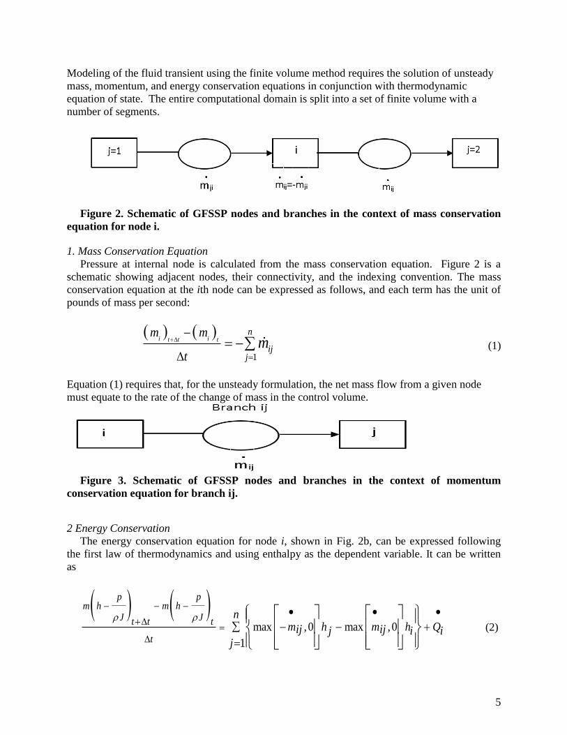
Figure 2. Schematic of GFSSP nodes and branches in the context of mass conservation

equation for node i.

1. Mass Conservation Equation

Pressure at internal node is calculated from the mass conservation equation. Figure 2 is a

schematic showing adjacent nodes, their connectivity, and the indexing convention. The mass

conservation equation at the ith node can be expressed as follows, and each term has the unit of

pounds of mass per second:

1

i it t tn

ijj

m m

tm

(1)

Equation (1) requires that, for the unsteady formulation, the net mass flow from a given node

must equate to the rate of the change of mass in the control volume.

Figure 3. Schematic of GFSSP nodes and branches in the context of momentum

conservation equation for branch ij.

2 Energy Conservation

The energy conservation equation for node i, shown in Fig. 2b, can be expressed following

the first law of thermodynamics and using enthalpy as the dependent variable. It can be written

as

max ,0 max ,0

1

p pm h m h

J Jt t t

t

nm h m h Qij ijj i i

j

(2)

6

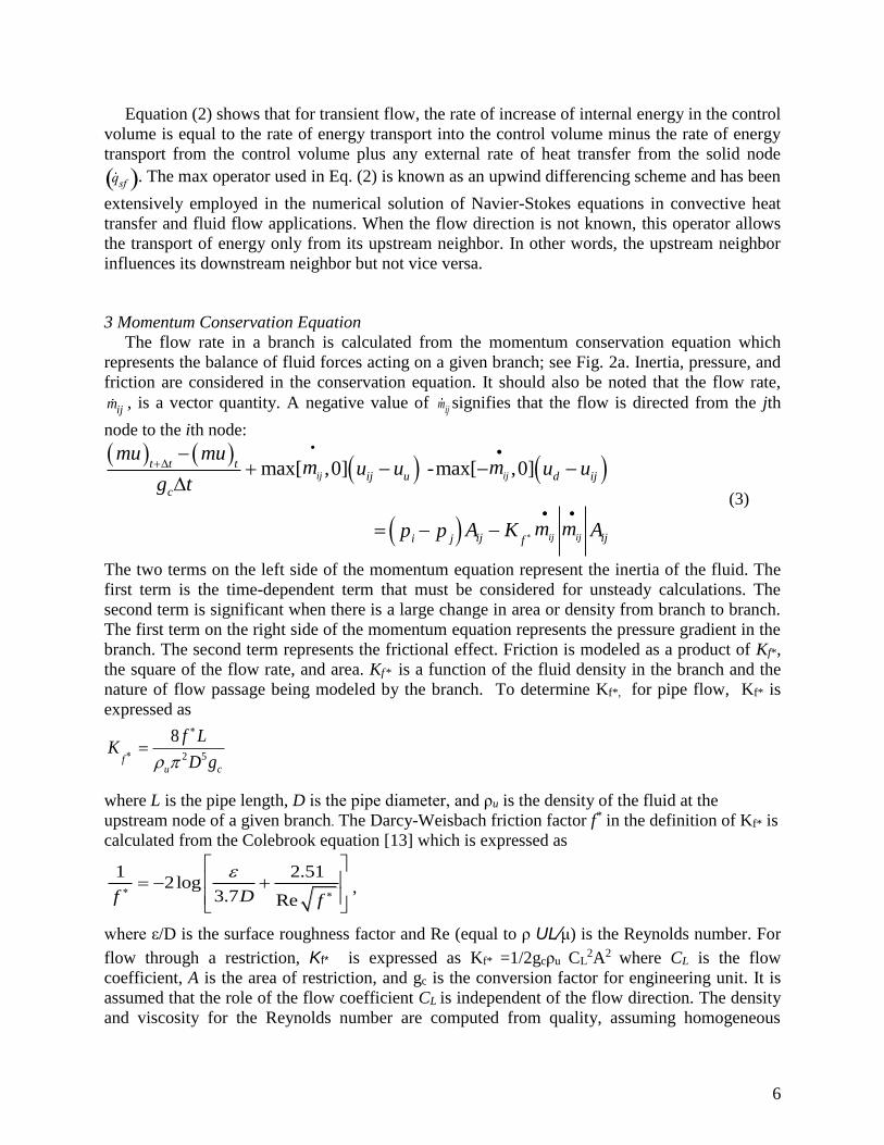
Equation (2) shows that for transient flow, the rate of increase of internal energy in the control

volume is equal to the rate of energy transport into the control volume minus the rate of energy

transport from the control volume plus any external rate of heat transfer from the solid node

qsf . The max operator used in Eq. (2) is known as an upwind differencing scheme and has been

extensively employed in the numerical solution of Navier-Stokes equations in convective heat

transfer and fluid flow applications. When the flow direction is not known, this operator allows

the transport of energy only from its upstream neighbor. In other words, the upstream neighbor

influences its downstream neighbor but not vice versa.

3 Momentum Conservation Equation

The flow rate in a branch is calculated from the momentum conservation equation which

represents the balance of fluid forces acting on a given branch; see Fig. 2a. Inertia, pressure, and

friction are considered in the conservation equation. It should also be noted that the flow rate,

ijm , is a vector quantity. A negative value of mij signifies that the flow is directed from the jth

node to the ith node:

max[ ,0] -max[ ,0]

ij ij

ij ij

t t tij u d ij

c

ij iji j f

mu mum mu u u u

g t

m mA K Ap p

(3)

The two terms on the left side of the momentum equation represent the inertia of the fluid. The

first term is the time-dependent term that must be considered for unsteady calculations. The

second term is significant when there is a large change in area or density from branch to branch.

The first term on the right side of the momentum equation represents the pressure gradient in the

branch. The second term represents the frictional effect. Friction is modeled as a product of Kf*,

the square of the flow rate, and area. Kf* is a function of the fluid density in the branch and the

nature of flow passage being modeled by the branch. To determine Kf*, for pipe flow, Kf* is

expressed as

2 5

8

fu c

f LK

D g

where L is the pipe length, D is the pipe diameter, and ρu is the density of the fluid at the

upstream node of a given branch. The Darcy-Weisbach friction factor f* in the definition of Kf* is

calculated from the Colebrook equation [13] which is expressed as

1 2.512log

3.7 ReDf f

,

where ε/D is the surface roughness factor and Re (equal to ρ UL∕μ) is the Reynolds number. For

flow through a restriction, Kf* is expressed as Kf* =1/2gcρu CL2A2 where CL is the flow

coefficient, A is the area of restriction, and gc is the conversion factor for engineering unit. It is

assumed that the role of the flow coefficient CL is independent of the flow direction. The density

and viscosity for the Reynolds number are computed from quality, assuming homogeneous

7

mixture, to account for two phase flow. The momentum conservation equation also requires

knowledge of the density and the viscosity of the fluid within the branch. These are functions of

the temperatures, and pressures, and can be computed using the thermodynamic property

program in [11] that provides the thermodynamic and transport properties for different fluids.

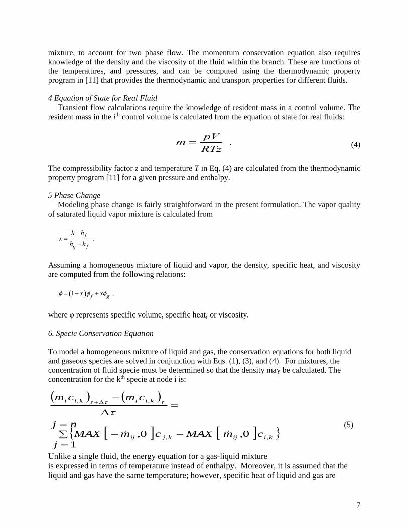
4 Equation of State for Real Fluid

Transient flow calculations require the knowledge of resident mass in a control volume. The

resident mass in the ith control volume is calculated from the equation of state for real fluids:

m pV

RTz. (4)

The compressibility factor z and temperature T in Eq. (4) are calculated from the thermodynamic

property program [11] for a given pressure and enthalpy.

5 Phase Change

Modeling phase change is fairly straightforward in the present formulation. The vapor quality

of saturated liquid vapor mixture is calculated from

x h h f

hg h f

.

Assuming a homogeneous mixture of liquid and vapor, the density, specific heat, and viscosity

are computed from the following relations:

1 x f xg .

where φ represents specific volume, specific heat, or viscosity.

6. Specie Conservation Equation

To model a homogeneous mixture of liquid and gas, the conservation equations for both liquid

and gaseous species are solved in conjunction with Eqs. (1), (3), and (4). For mixtures, the

concentration of fluid specie must be determined so that the density may be calculated. The

concentration for the kth specie at node i is:

1

0, 0, ,,

,,

nj

j

cmMAXcmMAX

cmcm

kiijkjij

kiikii

(5)

Unlike a single fluid, the energy equation for a gas-liquid mixture

is expressed in terms of temperature instead of enthalpy. Moreover, it is assumed that the

liquid and gas have the same temperature; however, specific heat of liquid and gas are

8

evaluated from a thermodynamic property program [11]. The density, specific heat, and

viscosity of the mixture are then calculated.

7. Energy Conservation Equation for Solid

In fluid-solid network for conjugate heat transfer, solid nodes, ambient nodes, and conductors

become part of the flow network. A typical flow network for conjugate heat transfer is shown in

Fig. 2b. The energy conservation equation for the solid node is solved in conjunction with all

other conservation equations. The energy conservation for solid node i can be expressed as:

1 1 1

( ) ( )

sfss sa

s f a

i i nn np s t t p s t

iss sf sa

j j j

mC T mC Tq q q S

t

(6)

The left-hand side of the equation represents rate of change of temperature of the solid node, i.

The right-hand side of the equation represents the heat transfer from the neighboring node and

heat source or sink. The heat transfer from neighboring solid, fluid, and ambient nodes can be

expressed as follows:

qss kijsAij

s/ ij

sTsjs Ts

i , (7a)

qsf hij f Aijs T fj f Ts

i , (7b)

and

qsa hijaAij

aTaja Ts

i . (7c)

The heat transfer rate can be expressed as a product of conductance and temperature differential.

The conductance for Eqs. (5a)–(5c) is

C ijskijsAij

s

ijs

; Cijf hij

fAij

f; Cij

a hij

aAij

a, (7d)

where effective heat transfer coefficients for solid to fluid and solid to ambient nodes are

expressed as:

hij

a hc,ij

a hr,ij

a,

hr,ij f

Tf

j f 2

Tsi 2

T f

j f Tsi

1

ij, f1

ij,s1

,

and

9

hr,ija

Tf

ja 2

Tsi 2

Ta

ja Ts

i

1

ij,a1

ij,s1

.

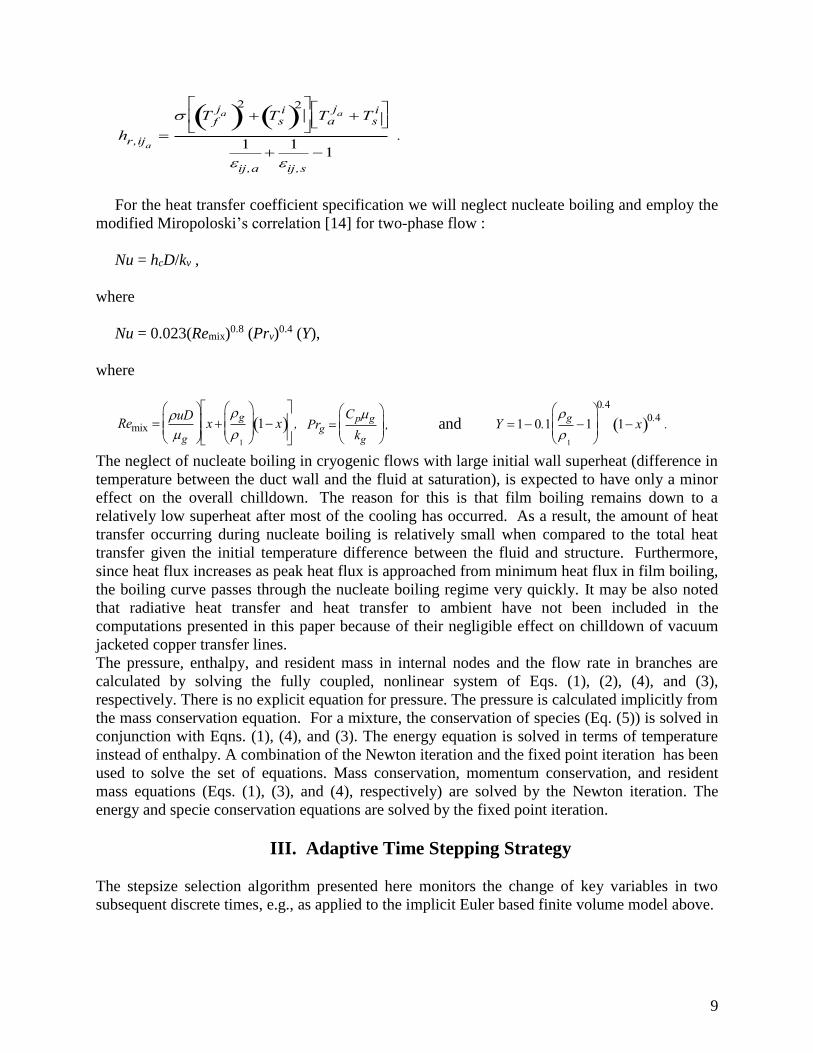
For the heat transfer coefficient specification we will neglect nucleate boiling and employ the

modified Miropoloski’s correlation [14] for two-phase flow :

Nu = hcD/kv ,

where

Nu = 0.023(Remix)0.8 (Prv)

0.4 (Y),

where

Remix uD

g

x

g

1

1 x

, Prg

Cpg

kg

, and Y 1 0.1

g

1

1

0.4

1 x 0.4.

The neglect of nucleate boiling in cryogenic flows with large initial wall superheat (difference in

temperature between the duct wall and the fluid at saturation), is expected to have only a minor

effect on the overall chilldown. The reason for this is that film boiling remains down to a

relatively low superheat after most of the cooling has occurred. As a result, the amount of heat

transfer occurring during nucleate boiling is relatively small when compared to the total heat

transfer given the initial temperature difference between the fluid and structure. Furthermore,

since heat flux increases as peak heat flux is approached from minimum heat flux in film boiling,

the boiling curve passes through the nucleate boiling regime very quickly. It may be also noted

that radiative heat transfer and heat transfer to ambient have not been included in the

computations presented in this paper because of their negligible effect on chilldown of vacuum

jacketed copper transfer lines.

The pressure, enthalpy, and resident mass in internal nodes and the flow rate in branches are

calculated by solving the fully coupled, nonlinear system of Eqs. (1), (2), (4), and (3),

respectively. There is no explicit equation for pressure. The pressure is calculated implicitly from

the mass conservation equation. For a mixture, the conservation of species (Eq. (5)) is solved in

conjunction with Eqns. (1), (4), and (3). The energy equation is solved in terms of temperature

instead of enthalpy. A combination of the Newton iteration and the fixed point iteration has been

used to solve the set of equations. Mass conservation, momentum conservation, and resident

mass equations (Eqs. (1), (3), and (4), respectively) are solved by the Newton iteration. The

energy and specie conservation equations are solved by the fixed point iteration.

III. Adaptive Time Stepping Strategy

The stepsize selection algorithm presented here monitors the change of key variables in two

subsequent discrete times, e.g., as applied to the implicit Euler based finite volume model above.

10

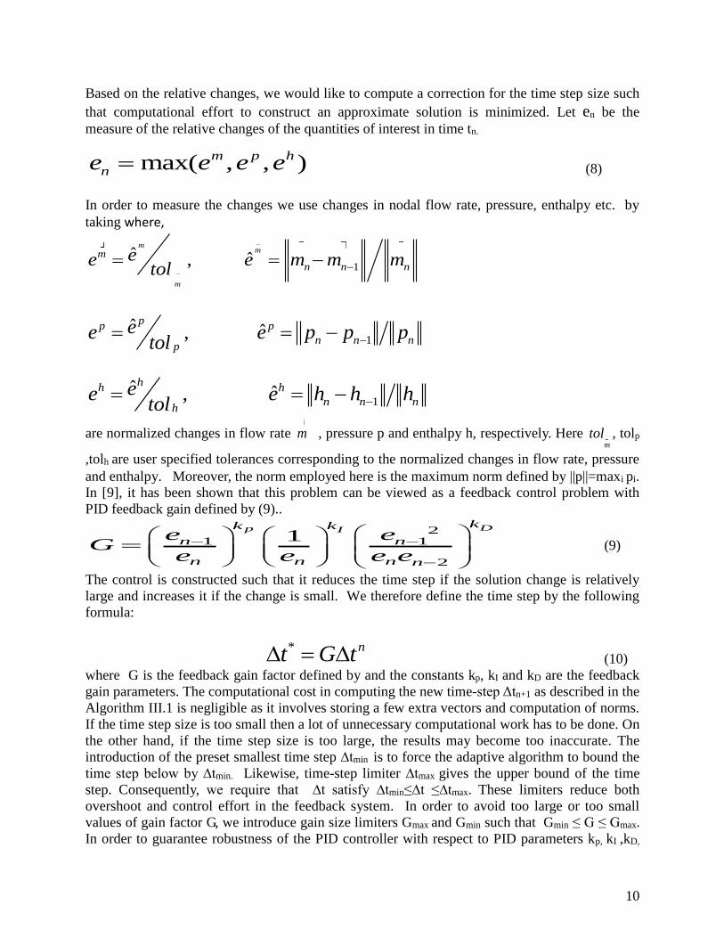
Based on the relative changes, we would like to compute a correction for the time step size such

that computational effort to construct an approximate solution is minimized. Let en be the

measure of the relative changes of the quantities of interest in time tn.

max( , , )m p h

ne e e e (8)

In order to measure the changes we use changes in nodal flow rate, pressure, enthalpy etc. by

taking where,

1ˆ ˆ,

mm

m

m

n n nee e m m m

tol

1ˆ ˆ,

pp p

n n np

ee e p p ptol

1ˆ ˆ,

hh h

n n nh

ee e h h htol

are normalized changes in flow rate m , pressure p and enthalpy h, respectively. Here m

tol , tolp

,tolh are user specified tolerances corresponding to the normalized changes in flow rate, pressure

and enthalpy. Moreover, the norm employed here is the maximum norm defined by ||p||=maxi pi.

In [9], it has been shown that this problem can be viewed as a feedback control problem with

PID feedback gain defined by (9)..

21 1

2

1Dp I

kk k

n n

n n n n

e eG

e e e e

(9)

The control is constructed such that it reduces the time step if the solution change is relatively

large and increases it if the change is small. We therefore define the time step by the following

formula:

* nt G t (10)

where G is the feedback gain factor defined by and the constants kp, kI and kD are the feedback

gain parameters. The computational cost in computing the new time-step Δtn+1 as described in the

Algorithm III.1 is negligible as it involves storing a few extra vectors and computation of norms.

If the time step size is too small then a lot of unnecessary computational work has to be done. On

the other hand, if the time step size is too large, the results may become too inaccurate. The

introduction of the preset smallest time step ∆tmin is to force the adaptive algorithm to bound the

time step below by ∆tmin. Likewise, time-step limiter ∆tmax gives the upper bound of the time

step. Consequently, we require that ∆t satisfy ∆tmin≤∆t ≤∆tmax. These limiters reduce both

overshoot and control effort in the feedback system. In order to avoid too large or too small

values of gain factor G, we introduce gain size limiters Gmax and Gmin such that Gmin ≤ G ≤ Gmax.

In order to guarantee robustness of the PID controller with respect to PID parameters kp, kI ,kD,

11

parametric studies were performed for different values of the parameters for two example

problems. The PID controller was found to be robust for kp=0.11075, kI =0.2625,kD =0.0165.

Algorithm III.1

i. Input: nm , p, h, ∆tmin, ∆tmax,kp,kI,kD, tol

nm , tolp, tolh, Gmax, Gmin

ii Initialize variables: en-2=1.d0,en-1=1.d0, ∆tn=∆tmin

ii. Compute en using (8) and compute G*using (9)

iii. Set G=max(G*,Gmin) and G=min(G*,Gmax)

iv. Compute ∆t*using (10)

v. Set ∆t=max(∆t*,∆tmin) and ∆t=min(∆t*,∆tmax)

vi. Set ∆tn=∆t

IV. Numerical Results In this section, we present two numerical experiments to test the adaptive time stepping scheme

presented in Algorithm III.1.

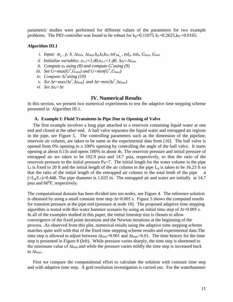
A. Example I: Fluid Transients in Pipe Due to Opening of Valve

The first example involves a long pipe attached to a reservoir containing liquid water at one

end and closed at the other end. A ball valve separates the liquid water and entrapped air regions

in the pipe, see Figure 5. The controlling parameters such as the dimension of the pipeline,

reservoir air column, are taken to be same as the experimental data from [16]. The ball valve is

opened from 0% opening to a 100% opening by controlling the angle of the ball valve. It starts

opening at about 0.15s and opens 100% in about 4s. The reservoir pressure and initial pressure of

entrapped air are taken to be 102.9 psia and 14.7 psia, respectively, so that the ratio of the

reservoir pressure to the initial pressure PR=7. The initial length for the water volume in the pipe

Ll is fixed to 20 ft and the initial length of the air column in the pipe Lg is taken to be 16.23 ft so

that the ratio of the initial length of the entrapped air column to the total lenth of the pipe α

(=Lg/LT)=0.448. The pipe diameter is 1.025 in. The entrapped air and water are initially at 14.7

psia and 600F, respectively.

The computational domain has been divided into ten nodes, see Figure 4. The reference solution

is obtained by using a small constant time step ∆t=0.005 s. Figure 5 shows the computed results

for transient pressure at the pipe end (pressure at node 10). The proposed adaptive time stepping

algorithm is tested with this water hammer scenario by using an initial time step of ∆t=0.005 s.

In all of the examples studied in this paper, the initial timestep size is chosen to allow

convergence of the fixed point iterations and the Newton iterations at the beginning of the

process. .As observed from this plot, numerical results using the adaptive time stepping scheme

matches quite well with that of the fixed time stepping scheme results and experimental data.The

time step is allowed to adjust between ∆tmin=0.001 and ∆tmax=0.01. The time history for the time

step is presented in Figure 8 (left). While pressure varies sharply, the time step is shortened to

the minimum value of ∆tmin and while the pressure varies mildly the time step is increased back

to ∆tmax .

First we compare the computational effort to calculate the solution with constant time step

and with adaptive time step. A grid resolution investigation is carried out. For the waterhammer

12

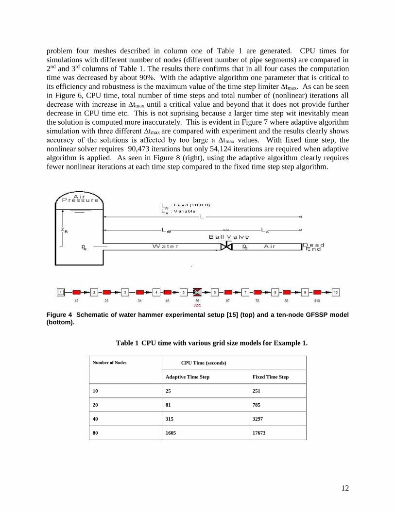
problem four meshes described in column one of Table 1 are generated. CPU times for

simulations with different number of nodes (different number of pipe segments) are compared in

2nd and 3rd columns of Table 1. The results there confirms that in all four cases the computation

time was decreased by about 90%. With the adaptive algorithm one parameter that is critical to

its efficiency and robustness is the maximum value of the time step limiter ∆tmax. As can be seen

in Figure 6, CPU time, total number of time steps and total number of (nonlinear) iterations all

decrease with increase in ∆tmax until a critical value and beyond that it does not provide further

decrease in CPU time etc. This is not suprising because a larger time step wit inevitably mean

the solution is computed more inaccurately. This is evident in Figure 7 where adaptive algorithm

simulation with three different ∆tmax are compared with experiment and the results clearly shows

accuracy of the solutions is affected by too large a ∆tmax values. With fixed time step, the

nonlinear solver requires 90,473 iterations but only 54,124 iterations are required when adaptive

algorithm is applied. As seen in Figure 8 (right), using the adaptive algorithm clearly requires

fewer nonlinear iterations at each time step compared to the fixed time step step algorithm.

Figure 4 Schematic of water hammer experimental setup [15] (top) and a ten-node GFSSP model (bottom).

Table 1 CPU time with various grid size models for Example 1.

Number of Nodes CPU Time (seconds)

Adaptive Time Step Fixed Time Step

10 25 251

20 81 785

40 315 3297

80 1605 17673

13

Figure 5. Predicted air pressure using adaptive time-stepping scheme for PR =7 at about

45% initial air volume (α=0.4491). Also shown are the predicted air pressure using fixed

time step and experimental data.

Figure 6. Effect of time step limiter ∆tmax on CPU time, total number of time steps and

total number of iterations

The time step limiters ∆tmax affects the CPU time, total number of iterations and total number

of time steps needed to complete the simulations. As we can see in Figure 6, CPU time, total

number of time steps and total number of iterations all decrease with increase in maximum time

step limiter ∆tmax . However, there seems to be a critical value beyond which increasing ∆tmax

14

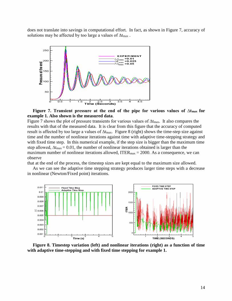
does not translate into savings in computational effort. In fact, as shown in Figure 7, accuracy of

solutions may be affected by too large a values of ∆tmax .

Figure 7. Transient pressure at the end of the pipe for various values of ∆tmax for

example 1. Also shown is the measured data.

Figure 7 shows the plot of pressure transients for various values of ∆tmax. It also compares the

results with that of the measured data. It is clear from this figure that the accuracy of computed

result is affected by too large a values of ∆tmax. Figure 8 (right) shows the time-step size against

time and the number of nonlinear iterations against time with adaptive time-stepping strategy and

with fixed time step. In this numerical example, if the step size is bigger than the maximum time

step allowed, ∆tmax = 0.01, the number of nonlinear iterations obtained is larger than the

maximum number of nonlinear iterations allowed, ITERmax = 2000. As a consequence, we can

observe

that at the end of the process, the timestep sizes are kept equal to the maximum size allowed.

As we can see the adaptive time stepping strategy produces larger time steps with a decrease

in nonlinear (Newton/Fixed point) iterations.

Figure 8. Timestep variation (left) and nonlinear iterations (right) as a function of time

with adaptive time-stepping and with fixed time stepping for example 1.

15

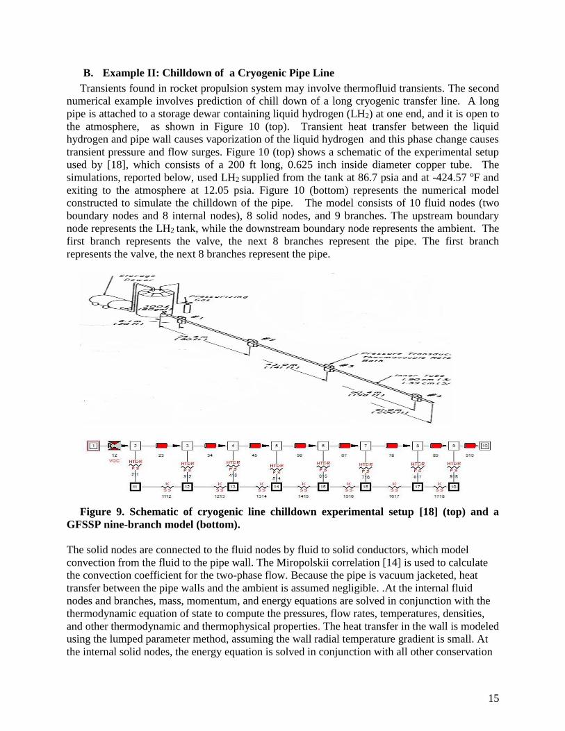
B. Example II: Chilldown of a Cryogenic Pipe Line

Transients found in rocket propulsion system may involve thermofluid transients. The second

numerical example involves prediction of chill down of a long cryogenic transfer line. A long

pipe is attached to a storage dewar containing liquid hydrogen (LH2) at one end, and it is open to

the atmosphere, as shown in Figure 10 (top). Transient heat transfer between the liquid

hydrogen and pipe wall causes vaporization of the liquid hydrogen and this phase change causes

transient pressure and flow surges. Figure 10 (top) shows a schematic of the experimental setup

used by [18], which consists of a 200 ft long, 0.625 inch inside diameter copper tube. The

simulations, reported below, used LH2 supplied from the tank at 86.7 psia and at -424.57 oF and

exiting to the atmosphere at 12.05 psia. Figure 10 (bottom) represents the numerical model

constructed to simulate the chilldown of the pipe. The model consists of 10 fluid nodes (two

boundary nodes and 8 internal nodes), 8 solid nodes, and 9 branches. The upstream boundary

node represents the LH2 tank, while the downstream boundary node represents the ambient. The

first branch represents the valve, the next 8 branches represent the pipe. The first branch

represents the valve, the next 8 branches represent the pipe.

Figure 9. Schematic of cryogenic line chilldown experimental setup [18] (top) and a

GFSSP nine-branch model (bottom).

The solid nodes are connected to the fluid nodes by fluid to solid conductors, which model

convection from the fluid to the pipe wall. The Miropolskii correlation [14] is used to calculate

the convection coefficient for the two-phase flow. Because the pipe is vacuum jacketed, heat

transfer between the pipe walls and the ambient is assumed negligible. .At the internal fluid

nodes and branches, mass, momentum, and energy equations are solved in conjunction with the

thermodynamic equation of state to compute the pressures, flow rates, temperatures, densities,

and other thermodynamic and thermophysical properties. The heat transfer in the wall is modeled

using the lumped parameter method, assuming the wall radial temperature gradient is small. At

the internal solid nodes, the energy equation is solved in conjunction with all other conservation

16

equations.

Figure 10. Comparison of transient temperature for subcooled LH2 for the driving

pressures 86.7 psia at four stations. Also shown is the measured data.

The reference results are calculated with constant time step ∆t=0.001s. The predicted

temperature history is shown in Figure 10. Stations one to four are nodes whose locations

correspond to four measurement locations in the experimental data. These stations are located at

20, 80, 140 and 200ft, respectively, downstream of the tank.

Figure 11. Timestep variation as a function of time with adaptive time-stepping and with

fixed time stepping for example 2.

17

These numerical predictions compare well to the measured temperatures. At this driving

pressure the pipe line chills down in about 60s. Small discrepancy exists between prediction and

experiments. This is partly due to coarseness of the network node—both solid and fluid—and

partly due to the heat transfer coefficient that affects the longitudinal conduction that can be seen

by noting that the discrepancy increases at each successive station in the downstream. As can be

seen in Figure 10, the numerical model tends to slightly overpredict the cooldown times. Likely

reasons for computational results not matching experimental results are (i) inaccuracy of

Miropolski heat transfer correlation (ii) representation of friction factor in two phase flow

assuming homogeneous mixture and (iii) uncertainty in the experimental data being compared

with.

The adaptive time stepping algorithm is tested with this problem by using an initial time step

of ∆t=0.001s. The time step is adjusted between ∆tmin=0.001s and ∆tmax=0.007s. The time

history for the time step is presented in Figure 11. Figure 10 compares the wall temperatures of

the adaptive time step predictions of the numerical model and the fixed time step predictions

over the course of a 100 s simulation. When the time step is adjusted according to the adaptive

algorithm between ∆tmin=0.001s and ∆tmax=0.007s, the accuracy of the results is as good as with

constant time step ∆t=0.001s. When the fluid touches the warm pipe walls, heat transfer causes

the liquid hydrogen to boil and the pipe wall temperature to rapidly decrease and the time step is

shortened by the adaptive scheme. As the pipe chills down to the liquid temperature the time

step is increased back to ∆tmax=0.007s.

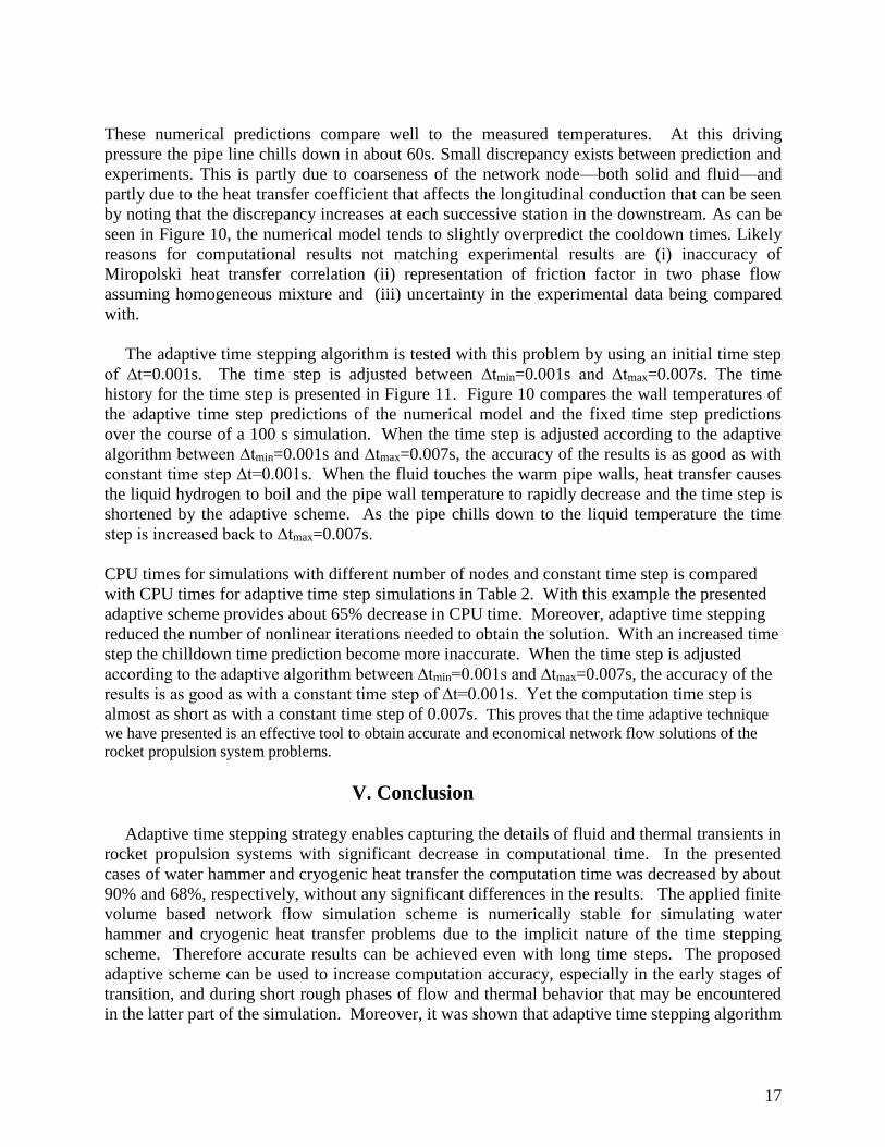
CPU times for simulations with different number of nodes and constant time step is compared

with CPU times for adaptive time step simulations in Table 2. With this example the presented

adaptive scheme provides about 65% decrease in CPU time. Moreover, adaptive time stepping

reduced the number of nonlinear iterations needed to obtain the solution. With an increased time

step the chilldown time prediction become more inaccurate. When the time step is adjusted

according to the adaptive algorithm between ∆tmin=0.001s and ∆tmax=0.007s, the accuracy of the

results is as good as with a constant time step of ∆t=0.001s. Yet the computation time step is

almost as short as with a constant time step of 0.007s. This proves that the time adaptive technique

we have presented is an effective tool to obtain accurate and economical network flow solutions of the

rocket propulsion system problems.

V. Conclusion

Adaptive time stepping strategy enables capturing the details of fluid and thermal transients in

rocket propulsion systems with significant decrease in computational time. In the presented

cases of water hammer and cryogenic heat transfer the computation time was decreased by about

90% and 68%, respectively, without any significant differences in the results. The applied finite

volume based network flow simulation scheme is numerically stable for simulating water

hammer and cryogenic heat transfer problems due to the implicit nature of the time stepping

scheme. Therefore accurate results can be achieved even with long time steps. The proposed

adaptive scheme can be used to increase computation accuracy, especially in the early stages of

transition, and during short rough phases of flow and thermal behavior that may be encountered

in the latter part of the simulation. Moreover, it was shown that adaptive time stepping algorithm

18

can also improve the convergence behavior of the nonlinear solver associated with the implicit

time stepping scheme leading to further reduction in CPU time.

The presented adaptive time stepping algorithm is a general one and can be applied for

network simulation study of transient thermos-fluid dynamic analysis of fluid systems and

components of importance to aerospace and other engineering industries.

Table 2 CPU time with various grid size models for Example 2

Acknowledgments

The work of S.S. Ravindran was supported in part by NASA grant #NNM16AA06A. This

author was also supported in part by a grant from NASA Tech Excellence Program. The part

work was conducted at Marshall Space Flight Center, Huntsville, Alabama, in the ER43/Thermal

Analysis Branch. The authors would like to thank the Thermal Analysis Branch for their support.

References

[1] Majumdar, A. K., and Steadman, T., “Numerical Modeling of Pressurization of a

Propellant Tank,” Journal of Propulsion and Power, Vol. 17, No.2, 2001, pp. 385–390.

[2] Cross, M. F., Majumdar, A. K., Bennett Jr., J. C., and Malla, R. B., “Modeling of Chill

Down in Cryogenic Transfer Lines,” Journal of Spacecraft and Rockets, Vol. 39, No. 2,

2002, pp. 284–289.

[3] Majumdar, A. and Ravindran, S.S., “Computational Modeling of Fluid and Thermal

Transients for Rocket Propulsion Systems by Fast Nonlinear Network Solver,” Int. J. Numer.

Method, Vol. 20, No. 6, 2010, pp. 617–637.

[4] Majumdar, A. and Ravindran, S.S.: “Numerical Modeling of Conjugate Heat Transfer in

Fluid Network,” J. Prop. Power, Vol. 27, No. 3, 2011, pp. 620–630.

[5] Gear, C.W., Numerical Initial Value Problems in Ordinary Differential Equations, Prentice

Hall, Englewood Cliff, N.J., 1971.

Number of Nodes CPU Time (seconds)

Adaptive Time Step Fixed Time Step

10 7,531 23,534

20 15,168 47,680

40 30,222 93,278

80 61,210 191,587

19

[6] Johnson, C., “Error Estimates and Adaptive Time Step Control for a Class of One Step

Methods for Stiff ODEs”, SIAM Journal of Numerical Analysis, Vol. 25, 1988, pp. 908-

926.

[7] Thomas, R.M. and Gladwell, I., “Variable-order variable-step algorithms for second order

systems-Part I: The method”, International Journal of Numerical Methods in Engineering,

Vol. 26, 1988, pp. 39-53.

[8] Zienkiewicz, O.C., Wood, W.L., Hine, N.W. and Taylor, R.L., “A unified one-step

algorithms-Part I: General formulations and Applications”, International Journal of

Numerical Methods in Engineering, Vol. 20, 1984, pp. 1529-1552.

[9] Gustafsson K, Lundh and M, Soderlind G., “A PI step-size control for the numerical solution

for ordinary differential equations”, BIT, Vol. 28, 1998, pp. 270–287.

[10] Majumdar, A. K., LeClair, A. C., Moore, R., and Schallhorn, P. A., Generalized Fluid

System Simulation Program, Version 6.0, NASA TM-2013-217492, Oct. 2013.

[11] Hendricks, R. C., Baron, A. K., and Peller, I. C., GASP—A Computer Code for Calculating

the Thermodynamic and Transport Properties for Ten Fluids: Parahydrogen, Helium, Neon,

Methane, Nitrogen, Carbon Monoxide, Oxygen, Fluorine, Argon, and Carbon Dioxide, NASA

TND-7808, Feb. 1975.

[12] Hendricks, R. C., Peller, I. C., and Baron, A. K., WASP—A Flexible Fortran IV Computer

Code for Calculating Water and Steam Properties, NASA TN-D-7391, Nov. 1973.

[13] Colebrook, C.F., “Turbulent flow in pipes, with particular reference to the transition region

between smooth and rough pipe laws”, Journal of the Institution of Civil Engineers, Vol.

11, 1939, pp. 133-156.

[14] Miropolski, Z. L., “Heat Transfer in Film Boiling of a Steam-Water Mixture in Steam

Generating Tubes”, Teploenergetika, Vol. 10, No. 5, 1963, pp. 49–52; transl. AEC-TR-

6252, 1964.

[15] Lee, N. H., and Martin, C. S., Experimental and Analytical Investigation of Entrapped Air

in a Horizontal Pipe, Proceedings of the 3rd ASME/JSME Joint Fluids Engineering Conference,

American Soc. Of Mechanical Engineers, Fairfield, NJ, July 1999, pp. 1–8.

[16] Lee, N. H., Effect of Pressurization and Expulsion of Entrapped Air in Pipelines, Ph.D.

Thesis, Georgia Inst. of Technology, Atlanta, Aug. 2005.

[17] Bandyopadhyay, A and Majumdar, A.K., “Network Flow Simulation of Fluid Transients in

Rocket Propulsion System”, Journal of Propulsion and Power, Vol. 30, No. 6, 2014, pp. 1646-

1653.

20

[18] Brennan, J. A., Brentari, E. G., Smith, R. V., and Steward, W. G., “Cooldown of Cryogenic

Transfer Lines—An Experimental Report,” National Bureau of Standards Report, 9264,

November 1966

[19] Gustafsson K, Soderlind G., “Control strategies for the iterative solution of nonlinear

equations in ODE solvers”, SIAM Journal of Scientific Computing, Vol. 18, No. 1, 1997,

pp. 23–40.

[20] Turek,S., “Efficient Solvers for Incompressible Flow Problems: An Algorithmic and

Computational Approach”, Lecture Notes in Computational Science and Engineering, Vol. 6,

Springer, 1999.

[21] Volker, J.,Rang,J., “Adaptive time step control for the incompressible Navier– Stokes

equations”, Comput. Methods Appl. Mech. Eng., Vol. 199, 2010, pp.514–524.

[22] Berrone, S.,and Marro,M., “Space–time adaptive simulations for unsteady Navier– Stokes

problems”, Computers and Fluids, Vol. 38, 2009, pp. 1132–1144.

[23] Gao, Z., Vassalos,D. and Gao,Q., “Numerical Simulation of Water Flooding into a

Damaged Vessel’s Compartment by Volume of Fluid Method”, J. Ocean Eng., Vol. 37, 2010,

pp. 1428–1442.

[24] Gresho Philip M., Griffiths David F., and Silvester David J., “Adaptive time-stepping for

incompressible flow. I. Scalar advection-diffusion”, SIAM J. Sci. Computing, Vol. 30, No. 4,

2008, pp. 2018- 2054.