Adaptive Radial Basis Function Methods for

Time Dependent Partial Differential

Equations

Scott A. Sarra

Department of Mathematics, Marshall University, One John Marshall Drive,Huntington, WV, 25755− 2560.

Abstract

Radial basis function (RBF) methods have shown the potential to be a universalgrid free method for the numerical solution of partial differential equations. Bothglobal and compactly supported basis functions may be used in the methods toachieve a higher order of accuracy. In this paper, we take advantage of the grid freeproperty of the methods and use an adaptive algorithm to choose the location ofthe collocation points. The RBF methods produce results similar to the more wellknown and analyzed spectral methods, but while allowing greater flexibility in thechoice of grid point locations. The adaptive RBF methods are most successful whenthe basis functions are chosen so that the PDE solution can be approximated wellwith a small number of the basis functions.

1 Introduction

Ultimately, we are interested in adaptive radial basis function (RBF) PDEalgorithms in two and three spatial dimensions. In this paper, we gain insightin one dimension before proceeding to higher dimensions. The implementationand complexity of RBF methods in higher dimensions are essentially the sameas in one dimension. Only the adaptive algorithm will need to be different.

RBF methods for time dependent PDEs enjoy large advantages in accuracyover other flexible, but low order methods, such finite differences, finite vol-umes, and finite elements. However, RBF methods share the ease of implemen-tation and flexibility of these lower order methods. Moving grid RBF methods

Email address: scott@scottsarra.org (Scott A. Sarra).URL: www.scottsarra.org (Scott A. Sarra).

Preprint submitted to Applied Numerical Mathematics 24 June 2004

are easily implemented, potentially even in complex computational domains inseveral space dimensions. Other highly accurate spatial discretization schemessuch as pseudospectral methods do not have the inherent flexibility of theRBF methods and adaptation and complex geometries are more difficult todeal with. We have applied a modification of a simple moving grid algorithm,which was developed for use with low order finite difference methods, to RBFmethods for time dependent PDEs. The adaptive RBF algorithm producesexcellent results.

The numerical solution of PDEs by RBF methods is based on a scattered datainterpolation problem which we review in this section. Let x0, x1, . . . , xN ∈Ω ⊂ Rn be a given set of centers. A radial basis function is a function φi(x) =φ(‖x− xi‖2), which depends only on the distance between x ∈ Rd and a fixedpoint xj ∈ Rd. Each function φj is radially symmetric about the center xj.The radial basis function interpolation problem may be described as, givendata fi = f(xi), i = 0, 1, . . . , N , the interpolating RBF approximation is

s(x) =N∑

i=0

λiφi(x) (1)

where the expansion coefficients, λi, are chosen so that s(xi) = fi. That is,they are obtained by solving the linear system

Hλ = f (2)

where the elements of the interpolation matrix are Hi,j = φ(‖xi − xj‖2), λ =[λ0, . . . , λN ]T , and f = [f0, . . . , fN ]T . For the RBFs that we have considered inthis work (table 1 and equation (8)), the interpolation matrix can be shownto be invertible for distinct interpolation points [21,26].

A generalized interpolation problem also may be considered. The generalizedinterpolation problem is

s(x) =N∑

i=0

λiφi(x) +M∑

k=1

bkpk(x) (3)

in which a finite number of d−variate polynomials of at most order M areadded to the RBF basis. The polynomials pk(x) are the polynomials spanningπM , that is they are the polynomials of degree at most M . The extra equa-tion(s) needed to complete the generalized interpolation problem are chosento be

N∑

j=0

λjpk(xj) = 0 (4)

2

for k = 1, . . . , M . Interpolation problem (3) must be considered when usingRBFs, such as the cubics φ(r) = r3, as the basic interpolation problem (1)does not lead to a guaranteed invertible interpolation matrix [22]. Also, thegeneralized interpolation problem may lead to an approximation with somedesirable properties that an approximation from the standard interpolationproblem may lack, such as a degree of polynomial accuracy. This is the casewith the multiquadric RBF [13].

Despite the fact that H can be shown to be invertible for all φ of the inter-est, the linear system (2) may often be very ill-conditioned and it may beimpossible to solve accurately using standard floating point arithmetic. Theconditioning of H is measured by the condition number defined as

κ(H) = ‖H‖∥∥∥H−1

∥∥∥ = σmax/σmin (5)

where σ are the singular values of H. The condition number of H is influencedby the number of centers, the minimum separation distance of the centers, aswell as values of parameters, defined below, such as the shape parameter andthe support.

2 Radial Basis Functions

The choice of basis function is another of the flexible features of RBF methods.We will review some properties of the RBFs that we use in the numerical ex-amples. RBFs can be globally supported, infinitely differentiable, and containa free parameter, ε, called the shape parameter. Representatives of this typeof RBF are listed in table 1. The global nature of RBFs of this type leads toa dense interpolation matrix. Global, infinitely differentiable RBFs typicallyinterpolate smooth data with spectral accuracy. Details can be found in thereferences [5,6,19,20].

The shape parameter affects both the accuracy of the approximation and theconditioning of the interpolation matrix. In general, for a fixed number of cen-ters N , smaller shape parameters produce the more accurate approximations,but also are associated with a poorly conditioned H. The condition numberalso grows with N for fixed values of the shape parameter ε. In practice, theshape parameter must be adjusted with the number of centers in order to pro-duce a interpolation matrix which is well conditioned enough to be invertedin finite precision arithmetic. Many researchers (e.g. [8,23]) have attemptedto develop algorithms for selecting optimal values of the shape parameter. Byoptimal, we mean the value of the shape parameter that produces the mostaccurate interpolant. However, results in this area have been limited by the re-alities of floating point arithmetic. The optimal choice of the shape parameter

3

is still an open question. In practice it is most often selected by brute force.Recently, Fornberg et. al. [12] developed a Contour-Pade algorithm which iscapable of stably computing the RBF approximation for all ε ≥ 0. The re-sults of using the Contour-Pade algorithm have shown that the optimal valueof the shape parameter may not be reachable in standard floating point pre-cision when applying traditional algorithms such as Gaussian elimination tosolve the system (2). Several different strategies [17] have been somewhatsuccessful in reducing the ill-conditioning problem when using RBF methodsin PDE problems. The strategies include: variable shape parameters, domaindecomposition, preconditioning the interpolation matrix, and optimizing thecenter locations. Often, more than one of these strategies are used together.

In our numerical examples, we have used the multiquadric (MQ) RBF which isdefined in table 1. Alternatively, the MQ may be defined as φ(r, c) =

√r2 + c2.

This is seen to be equivalent to our definition with ε = 1/c. It seems morenatural to define the MQ in this way rather than in the traditional way, asthe shape parameter now behaves in the same way it does in other infinitelysmooth RBFs. The behavior as ε → 0 is that the interpolant becomes moreaccurate, the condition number of the interpolation matrix gets larger, andthe shape of the RBF becomes flatter.

For approximation with the MQ RBF we consider the generalized interpolationproblem (3) with M = 1. The interpolation problem with M = 1 takes theform

s(x) =N∑

i=0

λiφi(x) + b (6)

where b is a constant and the auxiliary equation is

N∑

i=0

λi = 0. (7)

The resulting interpolation matrix will be of the form

H =

φ(‖x0 − x0‖2) · · · φ(‖x0 − xN‖2) 1...

. . ....

...

φ(‖xN − x0‖2) · · · φ(‖xN − xN‖2) 1

1 · · · 1 0

For the MQ the interpolation matrix constructed from the generalized interpo-lation problem with M = 1 is guaranteed to be invertible for distinct centers

4

Name of RBF Definition

Multiquadric (MQ) φ(r, ε) =√

1 + (εr)2

Inverse Quadratics (IQ) φ(r, ε) = 1/(1 + (εr)2)

Inverse Multiquadric (IMQ) φ(r, ε) = 1/√

1 + (εr)2

Gaussian (GA) φ(r, ε) = e−(εr)2

Table 1Global, infinitely smooth RBFs

[22]. For a discussion of the merits of using the MQ RBF with an appendedconstant see references [13] and [22].

An alternative to the global, infinitely smooth RBFs are compactly supportedRBFs (CSRBFs). Wendland’s CSRBFs [26] are representative of this class.The Wendland functions, φ`,κ, are strictly positive definite in Rd for all d ≤ d0

and can be constructed to have any desired amount of smoothness 2κ, i.e.,φ ∈ C2κ. The parameter ` is ` = bd

2c + κ + 1. For κ = 0, 1, 2, 3, the functions

can be computed by an explicit formulae [10]. The Wendland functions aredefined to have compact support on the interval [0, 1] but may be scaled tohave compact support on [0, δ] by replacing r with r/δ for δ > 0. The scalingfactor δ can be constant or it can be variable at different centers. A wayto specify the optimal value of δ is currently not known. In our numericalexperiments we have used the Wendland CSRBF

φ4,2 = (1− r)6+(3 + 18r + 35r2) (8)

where

(1− r)6+ =

(1− r)6+ 0 ≤ r < 1

0 r ≥ 1(9)

which are in C4 and are positive definite in up to three space dimensions. Sinceφ4,2 (W42) is positive definite we need only consider the standard interpolationproblem (1) and the matrix H will be nonsingular for a distinct set of centers.If the support of the basis functions are small compared to the size of thecomputational domain of the PDE, banded matrix algorithms can be usedto invert the interpolation matrix. Error estimates [27] for approximations off ∈ Hs(Rd) by Wendland’s CSRBFs are of the form

‖f − sf‖L∞(Ω) ≤ Chk+ 12 ‖f‖Hs(Rd) (10)

where h denotes the “meshsize”, i.e., the separation distance of the centers,h = supx∈Ω min ‖x− xj‖ for xj ∈ Rd. Hs(Rd) is the usual Sobolev space

5

of functions with s derivatives bounded in L2 and s = d2

+ k + 12

gives theregularity of the data.

3 RBF methods for time dependent PDEs

Derivatives of the interpolant (1) or (3) may be calculated in a straightforwardmanner. For instance, using the interpolant (1) in R, the derivatives at thecenters xj can be calculated as

s(n)(xj) =N∑

i=0

λiφ(n)i (xj). (11)

for n = 1, 2, . . .. The spatial derivatives can be written compactly in matrixform as

s(n) = H(n)λ (12)

where the elements of H(n) are φ(n)(‖xi − xj‖2).

In the context of a time dependent PDE method, where derivatives may needto be evaluated thousands of times, it is often more efficient to form thederivative matrix

D(n) = H(n)H−1. (13)

Then spatial derivatives can be approximated by a single matrix by vectormultiplication

s(n) = D(n)s. (14)

To describe how to implement a RBF method for solving a time dependentPDE on a fixed grid, we use Burgers’ equation (23) as an example. A fixedtime step has been used, but variable time stepping is possible. The PDE isdiscretized in space with radial basis functions to get the semi-discrete system

st = F (s). (15)

The system of ODEs (15) is then advanced in time with any ODE method. Inthe numerical examples, we have used an explicit fourth-order Runge-Kuttamethod. At time t = 0 the derivative matrixes, D(1) and D(2), are constructed.

6

At each internal Runge-Kutta stage, we calculate s(1) = D(1)s, s(2) = D(2)s,and then for i = 0, . . . , N , Fi = νs(2)(xi)− s(xi)s

(1)(xi). The implementationof the method is extremely simple.

4 Adaptive Grids

It has generally been accepted, at least for problems in one space dimension,that adaptive grid methods are capable of resolving PDE solutions that con-tain regions of rapid variation with acceptable accuracy and without using anexcessive number of grid points. Adaptive grid methods and applications inone space dimension, have been extensively studied. Many one-dimensionaladaptive grid algorithms for time-dependent PDEs in the context of finitedifference, finite element, and pseudospectral methods have been described.Details and further references may be found in [1,2,4,14–16]. The adaptive gridalgorithm that we have used is a slightly modification of the equidistributionof arclength algorithm for one dimensional systems of PDEs described in [24].We have modified the interpolation step, which used cubic polynomials at in-terior nodes and quadratic polynomials at the nodes next to the boundary, toinstead use the same RBFs used in the PDE solution at all nodes. Thus, themethod does not require any modifications near the boundaries.

This allows the adaptive RBF methods to maintain an overall high order ofaccuracy. When we apply the adaptive algorithm with second-order finite dif-ferences, we have retained the cubic interpolation step. The algorithm is simpleand computationally inexpensive in that it is not necessary to transform theoriginal PDE into a new coordinate system, or is it necessary to solve anadditional companion PDE to choose the coordinate system and node distri-bution. Other algorithms may result in different, and possibly “better” gridsbeing used, but for our purposes, the features of the RBF methods we wish toexamine will remain very similar, regardless of particular adaptive algorithmused.

In the adaptive algorithm, we start at time t0 with a uniform grid x0j . To

advance the PDE in time with the adaptive grid algorithm, we start by as-suming that at time level tn we have computed approximate solutions sn

j , bya radial basis function method, to the true solution u(xn

j , tn) on a grid xn

j ,where j = 0, . . . , N . Then, the RBF method is used on the grid xn

j to obtain

approximations sn+1j to u(xn

j , tn+1). Next, the points (xn

j , sn+1j ) are joined by

straight lines and the length θn+1 of the resulting polygon is computed. Thenthe points P n+1

j on the polygon are found which divide its total length intoN equal parts. The new nodes xn+1

j are found as the projection of P n+1j onto

the x-axis. Finally, sn+1j , the approximation to u(xn+1

j , tn+1), is computed byusing RBFs to interpolate the values (xn

j , sn+1j ) to (xn+1

j , sn+1j ).

7

The adaptive algorithm contains two parameters that control the adaptation.The parameter µ causes the adaptation to be performed every µ time steps.The parameter β controls the relative size of the largest and smallest gridspacings by ensuring that

maxi

hi ≤√

1 + β mini

hi (16)

where hi = xi − xi−1. When using the adaptive algorithm with CSRBFs, thebandwidth, b, of the interpolation matrix H will be

b =

⌊δ

minihi

⌋. (17)

The computational cost of choosing a new grid is relatively small. However,setting up the RBF method on the new grid involves constructing derivativematrices for the new grid. Thus, the setup costs of the adaptive method maybe prohibitive, unless the PDE solution can be approximated with a relativelysmall number of centers or unless CSRBFs are used which lead to a narrowlybanded interpolation matrix that can be efficiently inverted.

To obtain an accurate numerical approximation with RBFs and the adaptivegrid algorithm, we have found that a good strategy is to monitor the conditionnumber of the interpolation matrix H that is used to form new derivativematrices and to interpolate to the new set of centers each time the solutionis re-gridded. The condition number of H should not exceed 5 × 1010 duringany stage of the time evolution of the solution. If the condition number doesbecome too large, the stage should be rejected and recalculated with a smallervalue of β, which decreases the minimum separation distance of the centers.Another option to reduce the condition number of H for a rejected stage isto decrease the number of centers used. Both the values of β and N may beadapted when a re-gridding takes place. If it is not possible to achieve smallenough condition numbers in a single domain, domain decomposition will benecessary.

5 Numerical Results

First, we have applied the adaptive algorithm described in section 4 to select acomputational grid for a single derivative calculation. Then we have applied itto two PDE problems with solutions containing regions of rapid variation. Theresults are compared with pseudospectral and finite difference approximations.

The simple adaptive algorithm can be used in RBF methods to achieve an

8

accuracy goal, but with significantly fewer centers than a fixed grid methodwould require. In order to get a point of reference for the accuracy of RBFfunction methods on fixed grids, we compare the accuracy of the RBF functionmethods on fixed grids with the well known Chebyshev pseudospectral (CPS)method [7]. Additionally, we compare the RBF methods with a centered secondorder finite difference method (FD2) on both fixed and adaptive grids. Weillustrate the fact that the simple adaptive algorithm that we have applied inthe RBF and FD2 methods is not able to be applied in CPS method since themethod is restricted to a fixed grid or to mappings of that grid. This featureof the CPS method adds to the complexity of CPS adaptive algorithms andlimits the possible positioning of grid points.

For all the PDE methods we have taken small uniform time steps with a fourth-order explicit Runge-Kutta method in order to make the temporal errors small.In this way, we have isolated the effects of the spatial approximations as muchas possible. However, algorithms which adaptively adjust the time step couldbe used in conjunction with the adaptive spatial schemes to reduce the numberof time steps taken.

Two types of errors were measured, the max error

E∞ = max0≤i≤N

|f(xi)− s(xi)| (18)

where f(x) is the exact value and s(x) is the RBF approximation, and therms error

E2 =

√√√√ 1

N

∑

0≤i≤N

|f(xi)− s(xi)|2. (19)

5.1 Single Derivative

Our first numerical experiment compares the accuracy of the RBF methodsand the CPS method for calculating a single derivative of a function with aregion of rapid variation. The comparison is made on both fixed base gridsand on grids adapted based on qualities on the function being approximated.The function being differentiated is the exact solution to Burgers’ equation(23) from our second numerical example. We have used the solution at timet = 1.1 with ν = 0.01. In both the base grid and adapted grid calculationswe have used 50 grid points. RBF methods are not tied to a fixed grid, butwe take an evenly spaced grid as the “base” grid of the methods. We can notdo the same for the CPS method since methods that are based on high orderglobal polynomial interpolation are unstable on uniform grids. This situation

9

method E2 error

MQ base 0.056371

MQ adaptive 0.000087

CPS base 0.319269

CPSα = 0.99 0.109765

CPS adaptive 0.000093Table 2Single derivative results, N = 49

is often described by the term Runge phenomenon. Among several choices,the base grid for the CPS method is usually chosen to be

xj = −cos(πj

N), j = 0, 1, ..., N. (20)

The grid clusters nodes quadratically around the boundaries. The results ofthe base grid calculations are listed in table 2. The lack of resolution in centerof the domain caused by the boundary clustering of nodes leads to a largeerror in the CPS method. Often, the grid (20) is redistributed via a mappingof this grid in order to lessen stable explicit time stepping limits in a timedependent PDE method or to provide greater resolution in regions other thannear the boundaries. Perhaps the most used map is [18]

x =arcsin(αξ)

arcsin(α)(21)

which can produce a nearly evenly distributed set of grid points as α → 1,but is singular for α = 1. The results of using this map with α = 0.99 arelisted in the CPSα=0.99 row of table 2. The results are better than the CPSbase grid results, but not as good as the MQ RBF results on the uniform grid.For the MQ RBF, the shape parameter was selected as ε = 15. A remarkablefact about radial basis functions is that they can produce spectrally accurateresults to non-periodic problems on a uniform grid.

The simple adaptive algorithm that we have described in section 4 is applicableto both the RBF and FD2 methods, but can not be applied in the framework ofthe CPS method since the CPS method must be applied on its base grid (20),or on mapping of that grid. The simple adaptive algorithm does not accountfor this restriction, and more complex grid adaptation algorithms must beused for the CPS method.

Even though the adaptive algorithm we have used in the FD and RBF methodscan not be used in the CPS method, adaptive algorithms have been developed

10

for the CPS method. The adaptive CPS methods typically write the PDE ina transformed variable ξ through a mapping x = f(ξ, p1, p2) where p1 is a pa-rameter that describes the location of the rapid variation and p2 is a parameterthat controls the magnitude of the coordinate contraction near x = p1. Thevalues of p1 and p2, and thus the grid point locations, are selected by mini-mizing a functional of the solution that is connected with the approximationerror. The functional is typically taken to be the norm of a weighted Sobolevspace such as H2

w, but other choices are possible [3]. The possible grids arelimited to mappings of the grid (20). This grid dependence makes the CPSadaptive algorithms difficult to apply to problems with multiple regions ofrapid variation and hinders extension to higher space dimensions. Althoughthe mapping used may redistribute the grid points (20) to the interior of thedomain and to regions of rapid variation, some boundary clustering will stillbe present. Additionally, the CPS adaptive algorithms require a multidimen-sional optimization step which adds to the complexity of the methods. Thefull description of the adaptive CPS algorithm for PDEs is beyond the scopeof this work and the interested reader is referred to [2] for details and for anapplication of the adaptive CPS methods to Burgers’ equation. Here we onlyapply to method to a single derivative calculation. A map that is commonlyused in the CPS adaptive algorithms is

x = f(ξ, p1, p2) = p1 + p2 tan[ω(ξ − ξ0)] (22)

where ξ0 = (κ − 1)/(κ + 1), κ = tan−1([1 + p1]/p2)/ tan−1([1 − p1]/p2), andω = tan−1([1 − p1]/p2)/(1 − ξ0). The adaptive grid results are given in table2. The MQ RBF grid was produced by the algorithm described in section 4.The shape parameter used was ε = 15 and the grid adaption parameter wasβ = 18. The CPS adaptive grid was produced by minimizing a functionalbased on the H2

w norm to select the parameters p1 and p2 in map (22). Themethod selects the parameters as p1 ≈ 0 and p2 ≈ 5.3. The base and adaptedgrids for the single derivative test are shown in figure 1.

The results of this simple test of calculating a single derivative illustrate sev-eral features of RBF methods. One is that they can be as accurate as spectralmethods. RBF methods are grid free which allows center locations to be se-lected without restriction. Additionally, and important feature of RBF meth-ods that is sometimes overlooked is that they can produce spectral accuracyon a uniform grid.

11

method N E2 E∞ supp ε

MQ 103 0.00196 0.0092 - 11

W42 103 0.00159 0.0129 2 -

W42 103 0.00183 0.0159 0.6 -

FD2 340 0.00198 0.01889 - -

CPSα=0.99 113 0.00181 0.0068 - -

MQα=0.99 113 0.00173 0.0082 - 10

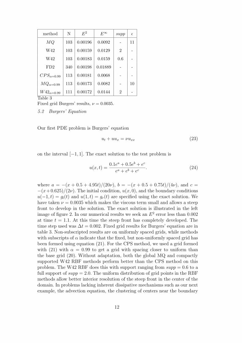
W42α=0.99 111 0.00172 0.0144 2 -Table 3Fixed grid Burgers’ results, ν = 0.0035.

5.2 Burgers’ Equation

Our first PDE problem is Burgers’ equation

ut + uux = νuxx (23)

on the interval [−1, 1]. The exact solution to the test problem is

u(x, t) =0.1ea + 0.5eb + ec

ea + eb + ec. (24)

where a = −(x + 0.5 + 4.95t)/(20ν), b = −(x + 0.5 + 0.75t)/(4ν), and c =−(x+0.625)/(2ν). The initial condition, u(x, 0), and the boundary conditionsu(−1, t) = gl(t) and u(1, t) = gr(t) are specified using the exact solution. Wehave taken ν = 0.0035 which makes the viscous term small and allows a steepfront to develop in the solution. The exact solution is illustrated in the leftimage of figure 2. In our numerical results we seek an E2 error less than 0.002at time t = 1.1. At this time the steep front has completely developed. Thetime step used was ∆t = 0.002. Fixed grid results for Burgers’ equation are intable 3. Non-subscripted results are on uniformly spaced grids, while methodswith subscripts of α indicate that the fixed, but non-uniformly spaced grid hasbeen formed using equation (21). For the CPS method, we used a grid formedwith (21) with α = 0.99 to get a grid with spacing closer to uniform thanthe base grid (20). Without adaptation, both the global MQ and compactlysupported W42 RBF methods perform better than the CPS method on thisproblem. The W42 RBF does this with support ranging from supp = 0.6 to afull support of supp = 2.0. The uniform distribution of grid points in the RBFmethods allow better interior resolution of the steep front in the center of thedomain. In problems lacking inherent dissipative mechanisms such as our nextexample, the advection equation, the clustering of centers near the boundary

12

method N β µ E2 E∞ supp ε

MQ 47 35 12 0.00191 0.00947 - 52

W42 60 30 10 0.00175 0.00670 2 -

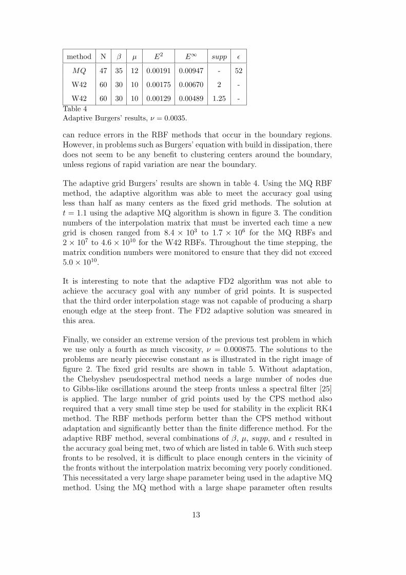
W42 60 30 10 0.00129 0.00489 1.25 -Table 4Adaptive Burgers’ results, ν = 0.0035.

can reduce errors in the RBF methods that occur in the boundary regions.However, in problems such as Burgers’ equation with build in dissipation, theredoes not seem to be any benefit to clustering centers around the boundary,unless regions of rapid variation are near the boundary.

The adaptive grid Burgers’ results are shown in table 4. Using the MQ RBFmethod, the adaptive algorithm was able to meet the accuracy goal usingless than half as many centers as the fixed grid methods. The solution att = 1.1 using the adaptive MQ algorithm is shown in figure 3. The conditionnumbers of the interpolation matrix that must be inverted each time a newgrid is chosen ranged from 8.4 × 103 to 1.7 × 106 for the MQ RBFs and2 × 107 to 4.6 × 1010 for the W42 RBFs. Throughout the time stepping, thematrix condition numbers were monitored to ensure that they did not exceed5.0× 1010.

It is interesting to note that the adaptive FD2 algorithm was not able toachieve the accuracy goal with any number of grid points. It is suspectedthat the third order interpolation stage was not capable of producing a sharpenough edge at the steep front. The FD2 adaptive solution was smeared inthis area.

Finally, we consider an extreme version of the previous test problem in whichwe use only a fourth as much viscosity, ν = 0.000875. The solutions to theproblems are nearly piecewise constant as is illustrated in the right image offigure 2. The fixed grid results are shown in table 5. Without adaptation,the Chebyshev pseudospectral method needs a large number of nodes dueto Gibbs-like oscillations around the steep fronts unless a spectral filter [25]is applied. The large number of grid points used by the CPS method alsorequired that a very small time step be used for stability in the explicit RK4method. The RBF methods perform better than the CPS method withoutadaptation and significantly better than the finite difference method. For theadaptive RBF method, several combinations of β, µ, supp, and ε resulted inthe accuracy goal being met, two of which are listed in table 6. With such steepfronts to be resolved, it is difficult to place enough centers in the vicinity ofthe fronts without the interpolation matrix becoming very poorly conditioned.This necessitated a very large shape parameter being used in the adaptive MQmethod. Using the MQ method with a large shape parameter often results

13

method N E2 E∞ supp ε ∆t

MQ 299 0.00179 0.01543 - 21 0.001

W42 339 0.00191 0.02696 0.8 - 0.002

FD2 1000 0.00193 0.0369 - - 0.0005

CPSα=0.99 429 0.00157 0.0206 - - 0.000025Table 5Fixed grid Burgers’ results, ν = 0.000875,

method N β µ E2 E∞ supp ε ∆t

MQ 139 100 20 0.00196 0.007455 - 110 0.0005

W42 149 20 10 0.00177 0.00938 0.8 - 0.002Table 6Adaptive Burgers’ results, ν = 0.000875.

in accuracy comparable to lower order finite difference methods. However,despite the large shape parameter, the MQ method produced good resultswhile the adaptive FD2 algorithm was unable to meet the accuracy goal withany number of grid points.

5.3 Advection Equation

Our next numerical experiment is with the advection equation

ut + ux = 0 (25)

with initial condition u(x, 0) = e−2000(x+1)2 and boundary condition u(−1, t) =g(t) = e−2000t2 . In our numerical results we seek an E2 error less than 0.002at time t = 1.0 when the thin pulse has moved to the center of the domain.Table 7 gives results on fixed grids. A small time step of ∆t = 0.001 was used.Non-subscripted results are on uniformly spaced grids, while methods withsubscripts of α indicate that the fixed, but non-uniformly spaced grid has beenformed using equation (21). It is well known that the largest errors in RBFmethods occur near boundaries [11], especially in non-dissipative wave typeproblems such as the advection equation. The reduction of boundary errors inthis type of problem has become an active area of research. One possible wayto lessen the boundary errors is to cluster centers around the boundaries aspseudospectral methods do. The results of the boundary clustering of centerscan be seen in the MQα=0.99 and MQα=0.9975 results. With a properly chosengrid, both the CPS and the MQ RBF method can meet the accuracy goalwith N = 111. As expected, the second order finite difference method was notcompetitive with the RBF or CPS methods.

14

method N E2 E∞ supp ε

MQ 169 0.00193 0.01825 - 24

W42 267 0.00195 0.01934 2 -

W42 229 0.00192 0.01818 0.1 -

FD2 3700 0.00199 0.01716 - -

CPSα=0.99 111 0.00178 0.00621 - -

MQα=0.99 125 0.00189 0.00721 - 8.5

MQα=0.9975 111 0.00167 0.00198 - 6.4Table 7Fixed grid Advection results

method N β µ E2 E∞ supp ε

MQ 61 48 2 0.00197 0.00805 - 31

W42 49 500 2 0.00141 0.00395 0.07 -

FD2* 1250 150 10 0.00150 0.00925 - -Table 8Adaptive Advection results

Table 8 gives the adaptive grid results. A small time step of ∆t = 0.001was used except for the FD2, which required a smaller time step for stabilityand ∆t = 0.00025 was used. With the grid parameter β = 500 in the W42calculation, the largest grid spacing may be as much as 22 times larger thanthe smallest grid spacing. In figure 4 this wide grid spacing can be observedin the flat regions of the solution. Despite the fact that the MQ interpolant isspectrally accurate and that the W42 approximation has only a fixed algebraicconvergence rate, the W42 RBF was able to attain the accuracy goal with lessnodes than the MQ RBF. Heuristically, this can be explained by the fact thatwith a support of 0.07 the W42 RBFs have a shape similar to the features in thePDE solution, while the MQ does not mimic the features of the PDE solutionas well. This is in agreement with one of the basic tenants of approximationtheory - choose a basis in which a function can be well represented by a smallnumber of basis functions.

The condition numbers of the interpolation matrix that must be inverted eachtime a new grid is chosen ranged from 9.5× 107 to 3.4× 109 for the MQ basisfunctions and 1.0×102 to 2.1×106 for the W42 basis functions. The structureand sparse nature of the interpolation matrix for the adaptive W42 calculationat t = 1.0 with δ = 0.07 is shown in figure 5.

15

6 Conclusions

Radial Basis Function methods were used to solve two PDEs with solutionscontaining regions of rapid variation. Without the use of grid adaptation,the RBF methods were competitive in both accuracy and computational costwith the Chebyshev pseudospectral method. The inherent flexility of the RBFmethods allowed the node location to be chosen adaptively in a way that re-tained the desired accuracy, but used significantly fewer centers. This completefreedom choice of center location is lacking in pseudospectral methods, sinceadaptations are limited to mappings of a fixed, non-uniformly spaced grid.The gridless feature of RBF methods will allow PDEs with solutions havingmultiple regions of rapid variation, and problems in higher dimensions, to behandled equally as well. The ability of the RBF methods to use a fixed uni-formly space grid is another advantage of the RBF methods over the CPSmethod.

The choice of basis function is another flexible feature of RBF methods. Basisfunctions may have global or compact support and may have varying degreesof smoothness. It was found in our numerical results that the “best” choiceof basis function for a particular problem was one in which the shapes of thebasis functions best matched the shapes or features of the PDE solution. Thisallowed the solution to be approximated well with a small number of basisfunctions.

Our future research will be concerned with adaptive grid RBF methods in twoand three space dimensions. We will be concerned with both existing adaptivealgorithms and new algorithms specifically tailored to RBF methods. The closeconnection between RBFs and wavelets [9] will be explored with the goal ofusing wavelets to guide the adaptation.

References

[1] S. Adjerid and J. E. Flaherty. A moving finite element method witherror estimation and refinement for one-dimensional time dependent partialdifferential equations. SIAM Journal on Numerical Analysis, 23:778–796, 1986.

[2] J.M. Augenbaum. An adaptive pseudospectral method for discontinuousproblems. Applied Numerical Mathematics, 5:459–480, 1989.

[3] A. Bayliss, D. Gottlieb, B. J. Matkowsky, and M. Minkoff. An adaptive pseudo-spectral method for reaction-diffusion problems. Journal of ComputationalPhysics, 81:421–443, 1989.

[4] G. Beckett, J. Mackenzie, A. Ramage, and D. Sloan. On the numerical solution

16

of one-dimensional PDEs using adaptive methods based on equidistribution.Journal of Computational Physics, 167:372–392, 2001.

[5] M. D. Buhmann. Spectral convergence of multiquadric interpolation.Proceedings of the Edinburgh Mathematical Society, 36:319–333, 1993.

[6] Martin D. Buhmann. Radial Basis Functions. Cambridge University Press,2003.

[7] Claudio Canuto, M. Y. Hussaini, Alfio Quarteroni, and Thomas A. Zang.Spectral Methods for Fluid Dynamics. Springer-Verlag, New York, 1988.

[8] R. E. Carlson and T. A. Foley. The parameter r2 in multiquadric interpolation.Computers and Mathematics with Applications, 21(9):29–42, 1991.

[9] C. K. Chui, J. Stockler, and J. D. Ward. Analytic wavelets generated by radialfunction. Advances in computational mathematics, 5:95–123, 1996.

[10] G. E. Fasshauer. On smoothing for multilevel approximation with radial basisfunctions. In Charles Chui and Lary Schumaker, editors, Approximation TheoryIX. Vanderbilt University Press, 1998.

[11] B. Fornberg, T. Dirscol, G. Wright, and R. Charles. Observations on thebehavior of radial basis function approximations near boundaries. Computersand Mathematics with Applications, 43:473–490, 2002.

[12] B. Fornberg and G. Wright. Stable computation of multiquadric interpolantsfor all values of the shape parameter. To appear in Computers and Mathematicswith Applications, 2004.

[13] R. L. Hardy. Theory and applications of the multiquadric-biharmonic method.Computers and Mathematics with Applications, 19(8/9):163–208, 1990.

[14] D. Hawken, J. Gottlieb, and J. Hansen. Review of some adaptive node-movement techniques in finite element and finite difference solutions of PDEs.Journal of Computational Physics, 95:254, 1991.

[15] W. Huang and R.D. Russell. A moving collocation method for solving timedependent partial differential equations. Applied Numerical Mathematics,20:101–116, 1996.

[16] Leland Jameson. A wavelet-optimized, very high order adaptive grid and ordernumerical method. SIAM Journal on Scientific Computing, 19(6):1980–2013,1998.

[17] E. Kaansa and Y.C. Hon. Circumventing the ill-conditioning problem withmultiquadric radial basis fuctions: Applications to elliptic partial differentialequations. Computers and Mathematics with Applications, 39(7/8):123–137,2000.

[18] R. Kosloff and H. Tal-Ezer. A modified Chebyshev pseudospectral method withan O(1/N) time step restriction. Journal of Computational Physics, 104:457–469, 1993.

17

[19] W. R. Madych and S. A. Nelson. Error bounds for multiquadric interpolation.In C. Chui, L. Schumaker, and J. Ward, editors, Approximation Therory VI,pages 413–416. Academic Press, 1989.

[20] W. R. Madych and S. A. Nelson. Multivariate interpolation and conditionallypositive definite functions ii. Mathematics of Computation, 4(189):211–230,1990.

[21] C. Micchelli. Interpolation of scattered data: Distance matrices andconditionally positive definite functions. Constructive Approximation, 2:11–22,1986.

[22] M. Powell. The theory of radial basis function approximation in 1990.In W. Light, editor, Advances in Numerical Analysis, Vol. II: Wavelets,Subdivision Algorithms and Radial Functions. 1990.

[23] S. Rippa. An algorithm for selecting a good parameter c in radial basis functioninterpolation. Advances in Computational Mathematics, 11:193–210, 1999.

[24] J. Sanz-Serna and I. Christie. A simple adaptive technique for nonlinear waveproblems. Journal of Computational Physics, 67:348–360, 1986.

[25] H. Vandeven. Family of spectral filters for discontinuous problems. SIAMJournal of Scientific Computing, 6:159–192, 1991.

[26] H. Wendland. Piecewise polynomial, positive definite and compactly supportedradial funtions of minimal degree. Advances in Compuational Mathematics,4:389–396, 1995.

[27] H. Wendland. Error estimates for interpolation by compactly supported radialbasis functions of minimal degree. Journal of Approximation Theory, 93:258–272, 1998.

18

−1 −0.5 0 0.5 1

−16

−14

−12

−10

−8

−6

−4

−2

0

x

MQ base grid

MQ adaptive grid

CPS base grid

CPS adaptive grid

Fig. 1. Derivative of the solution of Burgers’ equation (23) with ν = 0.01 at t = 1.1.Also displayed are the grids from the numerical experiment of section 5.1 whichapproximates the derivative of the solution profile on base and adaptive grids usingthe MQ RBF method and the Chebyshev pseudospectral method.

−1 −0.5 0 0.5 1

0

0.2

0.4

0.6

0.8

1

t = 0

t = 1.1

ν = 0.0035

−1 −0.5 0 0.5 1

0

0.2

0.4

0.6

0.8

1

t = 0

t = 1.1

ν = 0.000875

Fig. 2. Exact solution of Burgers’ (23) equation (solid) from section 5.2 at t = 0and t = 1.1 (dashed). Left: ν = 0.0035. Right ν = 8.75e− 4.

19

−1 −0.5 0 0.5 1

0

0.2

0.4

0.6

0.8

1

x

u(x,

1.1)

Fig. 3. Exact solution of Burgers’ equation (solid) at t = 1.1 from section 5.2. Opencircles represent the center locations at time t = 1.1 using the MQ RBF and N = 47.Results of the numerical experiment are given in table 4.

−1 −0.5 0 0.5 1

0

0.2

0.4

0.6

0.8

1

x

u(x,

1.0)

Fig. 4. Exact advection equation solution (solid) at t = 1 from section 5.3. Opencircles represent the center locations at time t = 1 using the Wendland W42 RBFand N = 49. Results of the numerical experiment are given in table 8.

20

0 5 10 15 20 25 30 35 40 45 50

0

5

10

15

20

25

30

35

40

45

50

Fig. 5. Structure of the interpolation matrix H at time t = 1 with N = 49 from theW42 numerical solution of the advection equation from section 5.3 and figure 4.

21