Adaptive multigrid methods

G. Brethes(*)

(*)INRIA - Ecuador project Sophia-Antipolis, France(*) Lemma Engineering, France

Gautier.Brethes@inria.fr

September 11, 2013

Introduction

Au = f

We want to combine two ideas:Multigrid methods and Mesh adaptation

2 Approximation and metrics

Table of contents:

I. Multigrid methods

II. Hessian-based mesh adaptation

III. Full-multigrid anisotropic adaptive algorithm

IV. Test cases

3 Approximation and metrics

Multigrid methods

Historic

Dates back to sixties (Bakhvalov, Fedorenko).Well established theory (Hackbusch, 1985)Full-Multigrid Method (FMG):Soon identifies as one of the first O(N) solution algorithm.

4 Approximation and metrics

I.Multigrid methods

Theory

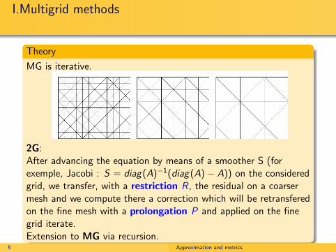
MG is iterative.

2G:After advancing the equation by means of a smoother S (forexemple, Jacobi : S = diag(A)−1(diag(A)− A)) on the consideredgrid, we transfer, with a restriction R, the residual on a coarsermesh and we compute there a correction which will be retransferedon the fine mesh with a prolongation P and applied on the finegrid iterate.Extension to MG via recursion.

5 Approximation and metrics

I. Multigrid methodsProperties of multigrids

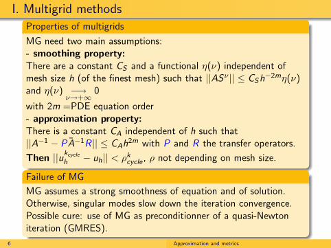
MG need two main assumptions:- smoothing property:There are a constant CS and a functional η(ν) independent ofmesh size h (of the finest mesh) such that ||ASν || ≤ CSh−2mη(ν)and η(ν) −→

ν→+∞0

with 2m =PDE equation order- approximation property:There is a constant CA independent of h such that||A−1 − PA−1R|| ≤ CAh2m with P and R the transfer operators.

Then ||ukcycle

h − uh|| < ρkcycle , ρ not depending on mesh size.

Failure of MG

MG assumes a strong smoothness of equation and of solution.Otherwise, singular modes slow down the iteration convergence.Possible cure: use of MG as preconditionner of a quasi-Newtoniteration (GMRES).

6 Approximation and metrics

I. Multigrid methods

Full-multigrid method

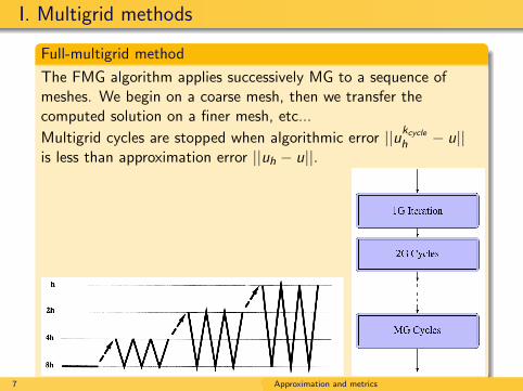
The FMG algorithm applies successively MG to a sequence ofmeshes. We begin on a coarse mesh, then we transfer thecomputed solution on a finer mesh, etc...

Multigrid cycles are stopped when algorithmic error ||ukcycle

h − u||is less than approximation error ||uh − u||.

7 Approximation and metrics

I. Multigrid methods

Full-multigrid method

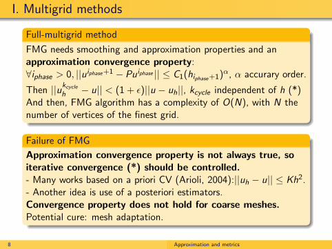
FMG needs smoothing and approximation properties and anapproximation convergence property:∀iphase > 0, ||uiphase+1 − Puiphase || ≤ C1(hiphase+1)α, α accurary order.

Then ||ukcycle

h − u|| < (1 + ε)||u − uh||, kcycle independent of h (*)And then, FMG algorithm has a complexity of O(N), with N thenumber of vertices of the finest grid.

Failure of FMG

Approximation convergence property is not always true, soiterative convergence (*) should be controlled.- Many works based on a priori CV (Arioli, 2004):||uh − u|| ≤ Kh2.- Another idea is use of a posteriori estimators.Convergence property does not hold for coarse meshes.Potential cure: mesh adaptation.

8 Approximation and metrics

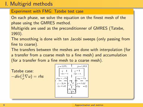
I. Multigrid methodsExperiment with FMG: Tatebe test case

On each phase, we solve the equation on the finest mesh of thephase using the GMRES method.Multigrids are used as the preconditionner of GMRES (Tatebe,1993).The smoothing is done with ten Jacobi sweeps (only passing fromfine to coarse).The transfers between the meshes are done with interpolation (fora transfer from a coarse mesh to a fine mesh) and accumulation(for a transfer from a fine mesh to a coarse mesh).

Tatebe case:−div( 1

ρ∇u) = rhs

9 Approximation and metrics

I. Multigrid methods

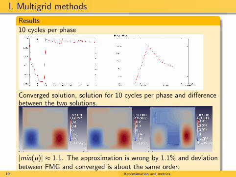
Results

10 cycles per phase

Converged solution, solution for 10 cycles per phase and differencebetween the two solutions.

|min(u)| ≈ 1.1. The approximation is wrong by 1.1% and deviationbetween FMG and converged is about the same order.

10 Approximation and metrics

II. Hessian-based mesh adaptation

Continuous mesh

Metric M: M(x) a matrix ∀x ∈ Ω.

Number of vertices: C(M) =

∫Ω

√det(M(x)) dx

Defining a Riemannian distance between two points:

dist(a,b) = lengthM(ab) =

∫ 1

0

√tabM(a + θab)ab dθ

HM =unit mesh for M ⇔ ∀ edge e ∈ HM, lengthM(e) ≈ 1

11 Approximation and metrics

II. Hessian-based mesh adaptation

Building the metric

An approximation uh of u, computed on a given mesh. Huhthe

Hessian.hi (x) = (λi (x))−1/2, with (λi (x))i=1,dim eigenvalues of Huh

(x).(vi (x))i=1,dim the eigenvectors of Huh

(x).Minimizing the error

εM = ||u − Πhu|| ≈∫

Ω

N∑i=1

hi (x)2(x)|tvi (x)Huh(x)vi (x)| dx

under the constraint: N =∫

Ω

√det(ML1(x)) dx.

The optimal metric field ML1(x) is given by:

ML1(x) = DLpdet(|Huh(x)|)

−15 |Huh

(x)|

where DL1 = N23 (

∫Ωdet(|Huh

(x)|)25 dx)

−23 .

Creation of a unit mesh for this metric.

12 Approximation and metrics

II. Hessian-based mesh adaptation

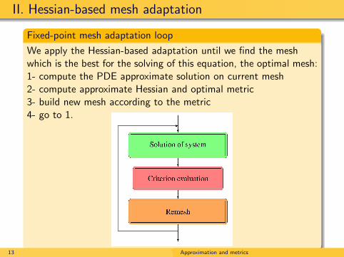
Fixed-point mesh adaptation loop

We apply the Hessian-based adaptation until we find the meshwhich is the best for the solving of this equation, the optimal mesh:1- compute the PDE approximate solution on current mesh2- compute approximate Hessian and optimal metric3- build new mesh according to the metric4- go to 1.

13 Approximation and metrics

III. Full-multigrid anisotropic adaptive algorithm

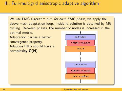
We use FMG algorithm but, for each FMG phase, we apply theabove mesh adaptation loop. Inside it, solution is obtained by MGcycling. Between phases, the number of nodes is increased in theoptimal metric.Adaptation carries a betterconvergence property.Adaptive FMG should have acomplexity O(N).

14 Approximation and metrics

IV. Test cases

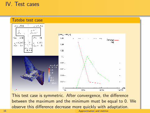
Tatebe test case

This test case is symmetric. After convergence, the differencebetween the maximum and the minimum must be equal to 0. Weobserve this difference decrease more quickly with adaptation.

15 Approximation and metrics

IV. Test cases

A stiff layer case

We observe the minimun tends to a limit value around 1.25 morequickly achieved with adaptation.

16 Approximation and metrics

Conclusion

Synthesis

MG combined with new mesh adaptation technology.

Introducing this more complex algorithm brings- a higher safety in the accuracy of results and- a better control of computational cost:

N = ε−dimα for obtaining a prescribed error ε.

Prospects

Convergence control of MG.

Convergence control of the adaptation loop.

A posteriori error estimator and corrector : uh ± δuh.

17 Approximation and metrics