ADAPTIVE MULTICAST ROUTING FOR MOBILE WIRELESS …cpj/publications/jaikaeo04adaptive.pdf ·...
181
ADAPTIVE MULTICAST ROUTING FOR MOBILE WIRELESS AD HOC NETWORKS by Chaiporn Jaikaeo A dissertation submitted to the Faculty of the University of Delaware in partial fulfillment of the requirements for the degree of Doctor of Philosophy in Computer and Information Sciences Summer 2004 c 2004 Chaiporn Jaikaeo All Rights Reserved
Transcript of ADAPTIVE MULTICAST ROUTING FOR MOBILE WIRELESS …cpj/publications/jaikaeo04adaptive.pdf ·...
ADAPTIVE MULTICAST ROUTING
FOR MOBILE WIRELESS AD HOC NETWORKS
by
Chaiporn Jaikaeo
A dissertation submitted to the Faculty of the University of Delaware inpartial fulfillment of the requirements for the degree of Doctor of Philosophy inComputer and Information Sciences
Summer 2004
c© 2004 Chaiporn JaikaeoAll Rights Reserved
ADAPTIVE MULTICAST ROUTING
FOR MOBILE WIRELESS AD HOC NETWORKS
by
Chaiporn Jaikaeo
Approved:M. Sandra Carberry, Ph.D.Chair of the Department of Computer and Information Sciences
Approved:Mark W. Huddleston, Ph.D.Dean of the College of Art and Sciences
Approved:Conrado M. Gempesaw II, Ph.D.Vice Provost for Academic and International Programs

I certify that I have read this dissertation and that in my opinion it meetsthe academic and professional standard required by the University as adissertation for the degree of Doctor of Philosophy.
Signed:Chien-Chung Shen, Ph.D.Professor in charge of dissertation
I certify that I have read this dissertation and that in my opinion it meetsthe academic and professional standard required by the University as adissertation for the degree of Doctor of Philosophy.
Signed:Adarshpal S. Sethi, Ph.D.Member of dissertation committee
I certify that I have read this dissertation and that in my opinion it meetsthe academic and professional standard required by the University as adissertation for the degree of Doctor of Philosophy.
Signed:Paul D. Amer, Ph.D.Member of dissertation committee
I certify that I have read this dissertation and that in my opinion it meetsthe academic and professional standard required by the University as adissertation for the degree of Doctor of Philosophy.
Signed:Charles G. Boncelet Jr., Ph.D.Member of dissertation committee
ADAPTIVE MULTICAST ROUTING
FOR MOBILE WIRELESS AD HOC NETWORKS
by
Chaiporn Jaikaeo
An abstract of a dissertation submitted to the Faculty of the Universityof Delaware in partial fulfillment of the requirements for the degree of Doctor ofPhilosophy in Computer and Information Sciences
Summer 2004
Approved:Chien-Chung Shen, Ph.D.Professor in charge of dissertation

ACKNOWLEDGMENTS
I owe special gratitude to my advisor, Professor Chien-Chung Shen, for his
advice, support and continuous encouragement in bringing this work to fruition.
I wish to thank my committee members, Professor Paul Amer, Professor Adarsh
Sethi, and Professor Charles Boncelet, for their valuable comments and feedbacks.
I am grateful to all of my present and former colleagues, Chavalit Srisathaporn-
phat, Zhuochuan Huang, Sonny Rajagopalan, Ozcan Koc, Ilknur Aydin, and Girish
Borkar, in our DEGAS networking group for their precious ideas and discussions. I
am also grateful to the department staff members, Pat Beazley, Fran D’Asaro, and
Vicki Cherry, for their great help.
I would like to express my deep gratitude to the Royal Thai Government
for the financial support throughout my graduate study and stay in the United
States. I seize this opportunity to convey my appreciation to Ruthalee and Robert
Carroll who have been encouraging me to meet many wonderful American friends
and learn many new things about American culture. I am especially grateful to my
loving fiance, Thitiwan Srinark, for her support during these years at University
of Delaware. I would also like to thank my former roommate, Kristian Link, who
always kept me entertained for the entire five years at College Towne Apartment.
Finally, but most importantly, I am deeply indebted to my parents and my
aunt for continuing to provide their love, support and encouragement throughout
my entire life.
iv
TABLE OF CONTENTS
LIST OF FIGURES . . . . . . . . . . . . . . . . . . . . . . . . . . . . . . . viiiLIST OF TABLES . . . . . . . . . . . . . . . . . . . . . . . . . . . . . . . . xivLIST OF ALGORITHMS . . . . . . . . . . . . . . . . . . . . . . . . . . . xvABSTRACT . . . . . . . . . . . . . . . . . . . . . . . . . . . . . . . . . . . xvi
Chapter
1 INTRODUCTION . . . . . . . . . . . . . . . . . . . . . . . . . . . . . . 12 BACKGROUND AND RELATED WORK . . . . . . . . . . . . . . 8
2.1 Multicast Techniques for Mobile Ad hoc Networks . . . . . . . . . . . 8
2.1.1 Taxonomy Based on Connectivity . . . . . . . . . . . . . . . . 9
2.1.1.1 Tree-based Protocols . . . . . . . . . . . . . . . . . . 92.1.1.2 Mesh-based Protocols . . . . . . . . . . . . . . . . . 11
2.1.2 Hierarchical, Hybrid and Adaptive Protocols . . . . . . . . . . 152.1.3 Other Classifications for Multicast Protocols . . . . . . . . . . 18
2.2 Biologically Inspired Algorithms for Computer Networks . . . . . . . 222.3 Wireless Communication with Directional Antennas . . . . . . . . . . 242.4 Summary . . . . . . . . . . . . . . . . . . . . . . . . . . . . . . . . . 25
3 ADAPTIVE DYNAMIC BACKBONE MULTICAST . . . . . . . . 27
3.1 Adaptive Dynamic Backbone (ADB) Protocol . . . . . . . . . . . . . 27
3.1.1 Local Data Structures . . . . . . . . . . . . . . . . . . . . . . 293.1.2 Neighbor Discovery Process . . . . . . . . . . . . . . . . . . . 303.1.3 Core Selection Process . . . . . . . . . . . . . . . . . . . . . . 34
v

3.1.4 Core Connection Process . . . . . . . . . . . . . . . . . . . . . 36
3.2 ADBM – Multicast Routing over ADB . . . . . . . . . . . . . . . . . 43
3.2.1 Group Joining . . . . . . . . . . . . . . . . . . . . . . . . . . . 433.2.2 Multicast Packet Forwarding . . . . . . . . . . . . . . . . . . . 45
3.3 Performance Evaluation . . . . . . . . . . . . . . . . . . . . . . . . . 45
3.3.1 Simulation Model . . . . . . . . . . . . . . . . . . . . . . . . . 463.3.2 Effects of Hop Threshold . . . . . . . . . . . . . . . . . . . . . 523.3.3 Effects of Path Stability Threshold . . . . . . . . . . . . . . . 523.3.4 Effect of Mobility . . . . . . . . . . . . . . . . . . . . . . . . . 593.3.5 Effects of Number of Senders . . . . . . . . . . . . . . . . . . 603.3.6 Effects of Multicast Group Size . . . . . . . . . . . . . . . . . 643.3.7 Effects of Traffic Load . . . . . . . . . . . . . . . . . . . . . . 67
3.4 Summary . . . . . . . . . . . . . . . . . . . . . . . . . . . . . . . . . 70
4 MULTICAST WITH SWARM INTELLIGENCE . . . . . . . . . . 72
4.1 Overview of MANSI . . . . . . . . . . . . . . . . . . . . . . . . . . . 734.2 MANSI Protocol Description . . . . . . . . . . . . . . . . . . . . . . . 79
4.2.1 Local Data Structures . . . . . . . . . . . . . . . . . . . . . . 794.2.2 Forwarding Set Initialization . . . . . . . . . . . . . . . . . . . 814.2.3 Forwarding Set Evolution . . . . . . . . . . . . . . . . . . . . 874.2.4 Multicast Data Forwarding . . . . . . . . . . . . . . . . . . . . 944.2.5 Handling Mobility . . . . . . . . . . . . . . . . . . . . . . . . 94
4.3 Experimental Results and Discussion . . . . . . . . . . . . . . . . . . 964.4 Summary . . . . . . . . . . . . . . . . . . . . . . . . . . . . . . . . . 105
5 A FRAMEWORK FOR EVOLUTIONARY MULTICASTROUTING . . . . . . . . . . . . . . . . . . . . . . . . . . . . . . . . . . 107
5.1 Evolutionary Multicast Routing Framework (EMRF) . . . . . . . . . 1085.2 Case Study: Integration of ADBM and MANSI . . . . . . . . . . . . 1125.3 Experimental Results and Discussion . . . . . . . . . . . . . . . . . . 1135.4 Summary . . . . . . . . . . . . . . . . . . . . . . . . . . . . . . . . . 121
vi
6 MULTICAST WITH DIRECTIONAL ANTENNAS . . . . . . . . 123
6.1 System Models . . . . . . . . . . . . . . . . . . . . . . . . . . . . . . 124
6.1.1 Directional Antenna Model . . . . . . . . . . . . . . . . . . . 1246.1.2 Signal Transmission and Reception Model . . . . . . . . . . . 125
6.2 Preliminary Experiment . . . . . . . . . . . . . . . . . . . . . . . . . 1276.3 Analysis on Signal Reception with Directional Antennas . . . . . . . 1356.4 Improving Delivery Success Rate . . . . . . . . . . . . . . . . . . . . 1436.5 Experiment with Acknowledgment . . . . . . . . . . . . . . . . . . . 1456.6 Summary . . . . . . . . . . . . . . . . . . . . . . . . . . . . . . . . . 149
7 CONCLUSION . . . . . . . . . . . . . . . . . . . . . . . . . . . . . . . . 151
7.1 Summary of Accomplishments . . . . . . . . . . . . . . . . . . . . . . 1517.2 Future Work . . . . . . . . . . . . . . . . . . . . . . . . . . . . . . . . 153
BIBLIOGRAPHY . . . . . . . . . . . . . . . . . . . . . . . . . . . . . . . . 155
vii
LIST OF FIGURES
1.1 Multicast operations with directional antennas: (a) Multicastpackets directionally sent to multiple members in the same sector,allowing another source to transmit a packet simultaneously, and (b)Multicast packet sent to multiple members located in differentsectors . . . . . . . . . . . . . . . . . . . . . . . . . . . . . . . . . . 3
1.2 Adaptability of multicast inherited from the adaptive backboneconstruction mechanism: more backbone nodes appear in a moredynamic area than the others of the network, causing a shift of theforwarding mechanism from tree-based forwarding to flooding inthat area . . . . . . . . . . . . . . . . . . . . . . . . . . . . . . . . 4
1.3 Examples of multicast connectivity among three group members(black circles): (a) six other nodes, shown in gray, establishing groupconnectivity and participating in multicast data forwarding, and (b)more efficient data forwarding when there are only four nodesforming group connectivity . . . . . . . . . . . . . . . . . . . . . . . 5
2.1 Examples of multicast connectivity in tree-based and mesh-basedapproaches (solid lines denote paths on which multicast packets areforwarded, and nodes in shade denote multicast group members):(a) a multicast tree, (b) a multicast mesh, and (c) a multicast fullmesh (flooding) . . . . . . . . . . . . . . . . . . . . . . . . . . . . 12
2.2 Classification of multicast protocols for ad hoc networks based onmember connectivity . . . . . . . . . . . . . . . . . . . . . . . . . . 17
3.1 Different backbone structures under different mobility speeds (thelarger black nodes represent the cores): (a) mobility speed is 0 m/s,and (b) mobility speed is 20 m/s. . . . . . . . . . . . . . . . . . . . 37
viii
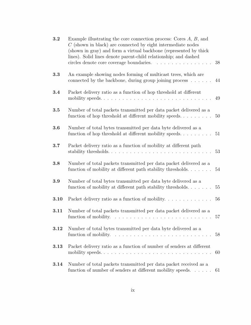
3.2 Example illustrating the core connection process: Cores A, B, andC (shown in black) are connected by eight intermediate nodes(shown in gray) and form a virtual backbone (represented by thicklines). Solid lines denote parent-child relationship; and dashedcircles denote core coverage boundaries. . . . . . . . . . . . . . . . 38
3.3 An example showing nodes forming of multicast trees, which areconnected by the backbone, during group joining process . . . . . . 44
3.4 Packet delivery ratio as a function of hop threshold at differentmobility speeds. . . . . . . . . . . . . . . . . . . . . . . . . . . . . . 49
3.5 Number of total packets transmitted per data packet delivered as afunction of hop threshold at different mobility speeds. . . . . . . . . 50
3.6 Number of total bytes transmitted per data byte delivered as afunction of hop threshold at different mobility speeds. . . . . . . . . 51
3.7 Packet delivery ratio as a function of mobility at different pathstability thresholds. . . . . . . . . . . . . . . . . . . . . . . . . . . . 53
3.8 Number of total packets transmitted per data packet delivered as afunction of mobility at different path stability thresholds. . . . . . . 54
3.9 Number of total bytes transmitted per data byte delivered as afunction of mobility at different path stability thresholds. . . . . . . 55
3.10 Packet delivery ratio as a function of mobility. . . . . . . . . . . . . 56
3.11 Number of total packets transmitted per data packet delivered as afunction of mobility. . . . . . . . . . . . . . . . . . . . . . . . . . . 57
3.12 Number of total bytes transmitted per data byte delivered as afunction of mobility. . . . . . . . . . . . . . . . . . . . . . . . . . . 58
3.13 Packet delivery ratio as a function of number of senders at differentmobility speeds. . . . . . . . . . . . . . . . . . . . . . . . . . . . . . 60
3.14 Number of total packets transmitted per data packet received as afunction of number of senders at different mobility speeds. . . . . . 61
ix
3.15 Number of total bytes transmitted per data byte received as afunction of number of senders at different mobility speeds. . . . . . 62
3.16 Packet delivery ratio as a function of group size at different mobilityspeeds. . . . . . . . . . . . . . . . . . . . . . . . . . . . . . . . . . . 64
3.17 Number of total packets transmitted per data packet received as afunction of group size at different mobility speeds. . . . . . . . . . . 65
3.18 Number of total bytes transmitted per data byte received as afunction of group size at different mobility speeds. . . . . . . . . . . 66
3.19 Packet delivery ratio as a function of traffic load at differentmobility speeds. . . . . . . . . . . . . . . . . . . . . . . . . . . . . . 67
3.20 Number of total packets transmitted per data packet received as afunction of traffic load at different mobility speeds. . . . . . . . . . 68
3.21 Number of total bytes transmitted per data byte received as afunction of traffic load at different mobility speeds. . . . . . . . . . 69
4.1 Examples of multicast connectivity among three group members:(a) a forwarding set of six nodes formed by shortest paths from thecore to the other two members, and (b) another forwarding set whennode A partially shares the same path to the core with node B,which results in more efficient data packet forwarding . . . . . . . . 75
4.2 Behavior of forward and backward ants: (1) a Forward Antdeployed from the member A choosing node C as the next hop andencountering a forwarding node D, and (2) at node D, theForward Ant becoming a Backward Ant and following thereverse path back to node A while depositing pheromone along theway . . . . . . . . . . . . . . . . . . . . . . . . . . . . . . . . . . . 77
4.3 An example illustrating how heights are assigned to forwardingnodes used by the members with IDs 3, 6 and 8 . . . . . . . . . . . 78
4.4 Sample network snapshots illustrating the operations of MANSI: (a)network setup with three members: nodes 1 (lower-left), 47(upper-right), and 50 (upper-left), where node 1 is the core, (b)dissemination of Core Announce indicated by arrows . . . . . . 83
x
4.5 Core Announce packet format . . . . . . . . . . . . . . . . . . . 85
4.6 Join Request packet format . . . . . . . . . . . . . . . . . . . . . 85
4.7 Ant packet format used by both Forward Ant and BackwardAnt . . . . . . . . . . . . . . . . . . . . . . . . . . . . . . . . . . . 87
4.8 A network of 50 nodes moving at 10 m/s, where members are inblack and forwarding nodes are in gray: (a) withoutmobility-adaptive mechanism, and (b) with mobility-adaptivemechanism where NLFF THRESHOLD is 0.01 . . . . . . . . . . . 97
4.9 Average size of the forwarding set as a function of time for COREand MANSI . . . . . . . . . . . . . . . . . . . . . . . . . . . . . . . 99
4.10 Packet delivery ratio as a function of mobility speed . . . . . . . . . 102
4.11 Total packets transmitted per data packet received at thedestinations as a function of mobility speed . . . . . . . . . . . . . 103
4.12 Total bytes transmitted per data byte received at the destinations asa function of mobility speed . . . . . . . . . . . . . . . . . . . . . . 104
5.1 Illustrations of initial multicast connectivity for four group membersusing different underlying infrastructures: (a) no infrastructure (i.e.,simple flooding), incurring a forwarding set of 8 nodes, (b) virtualbackbone, also resulting in 8 forwarding nodes, (c) single leader,resulting in 9 forwarding nodes, and (d) the optimal connectivity,requiring only 5 forwarding nodes . . . . . . . . . . . . . . . . . . . 111
5.2 Packet delivery ratio as a function of mobility speed . . . . . . . . . 118
5.3 Total packets transmitted per data packet received at thedestinations as a function of mobility speed . . . . . . . . . . . . . 119
5.4 Total bytes transmitted per data byte received at the destinations asa function of mobility speed . . . . . . . . . . . . . . . . . . . . . . 120
6.1 Top-view representation of transmission and reception gain for: (a)omni-directional antennas, and (b) M -sectorized directionalantennas . . . . . . . . . . . . . . . . . . . . . . . . . . . . . . . . . 124
xi
6.2 k out of M antenna sectors can be enabled simultaneously whiletransmitting a multicast packet to multiple receivers located indifferent sectors. . . . . . . . . . . . . . . . . . . . . . . . . . . . . 125
6.3 Average end-to-end packet delay as a function of the number ofsources under different communication modes . . . . . . . . . . . . 130
6.4 Overall throughput as a function of the number of sources underdifferent communication modes . . . . . . . . . . . . . . . . . . . . 131
6.5 Packet delivery ratio as a function of the number of sources underdifferent communication modes . . . . . . . . . . . . . . . . . . . . 132
6.6 Average number of signals dropped at the physical layer per node asa function of the number of sources under different communicationmodes . . . . . . . . . . . . . . . . . . . . . . . . . . . . . . . . . . 134
6.7 One-hop wireless communication model with communication radiusR and distance between the sender and the receiver x (x < R) . . . 135
6.8 Four modes of communication where solid curves representtransmission and reception regions of the sender A and the receiverB, and shaded areas represent unsafe regions: (a) Omni-directionalReception Omni-directional Transmission (OROT), (b) DirectionalReception Omni-directional Transmission (DROT), (c)Omni-directional Reception Directional Transmission (ORDT), and(d) Directional Reception Directional Transmission (DRDT) . . . . 137
6.9 Analytical probability of signal collision as a function ofomni-directional broadcast fraction (pomni) due to the presence ofunsafe regions in different communication modes . . . . . . . . . . 142
6.10 Data packet forwarding with acknowledgment in DRDT mode: (a)A broadcasts a multicast packet directionally to B and C, but onlyB can receive, (b) B acknowledges with an ACK packet, and (c) Atimes out and retransmits the same data packet only to the sector inwhich C is located . . . . . . . . . . . . . . . . . . . . . . . . . . . 145
6.11 Packet delivery ratio as a function of the number of sources underdifferent communication modes with and without acknowledgment . 146
xii

6.12 Overall throughput as a function of the number of sources underdifferent communication modes with and without acknowledgment . 147
6.13 Average end-to-end packet delay as a function of the number ofsources under different communication modes with and withoutacknowledgment . . . . . . . . . . . . . . . . . . . . . . . . . . . . 148
xiii
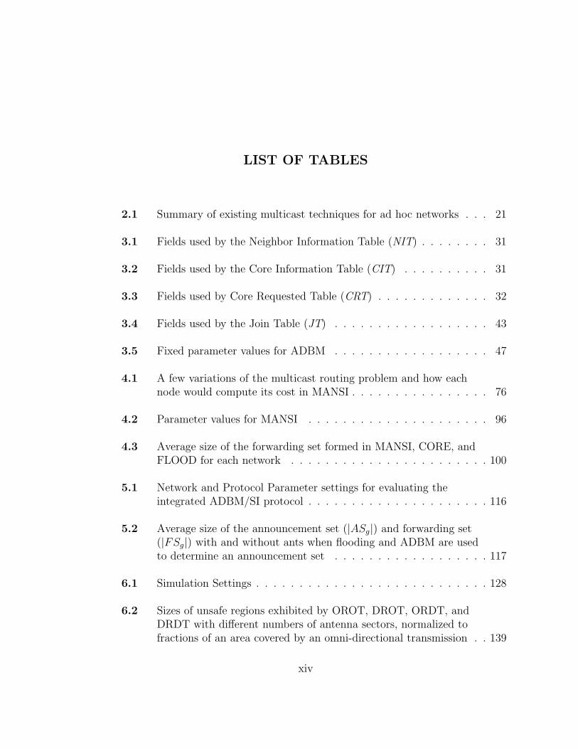
LIST OF TABLES
2.1 Summary of existing multicast techniques for ad hoc networks . . . 21
3.1 Fields used by the Neighbor Information Table (NIT) . . . . . . . . 31
3.2 Fields used by the Core Information Table (CIT) . . . . . . . . . . 31
3.3 Fields used by Core Requested Table (CRT) . . . . . . . . . . . . . 32
3.4 Fields used by the Join Table (JT) . . . . . . . . . . . . . . . . . . 43
3.5 Fixed parameter values for ADBM . . . . . . . . . . . . . . . . . . 47
4.1 A few variations of the multicast routing problem and how eachnode would compute its cost in MANSI . . . . . . . . . . . . . . . . 76
4.2 Parameter values for MANSI . . . . . . . . . . . . . . . . . . . . . 96
4.3 Average size of the forwarding set formed in MANSI, CORE, andFLOOD for each network . . . . . . . . . . . . . . . . . . . . . . . 100
5.1 Network and Protocol Parameter settings for evaluating theintegrated ADBM/SI protocol . . . . . . . . . . . . . . . . . . . . . 116
5.2 Average size of the announcement set (|ASg|) and forwarding set(|FSg|) with and without ants when flooding and ADBM are usedto determine an announcement set . . . . . . . . . . . . . . . . . . 117
6.1 Simulation Settings . . . . . . . . . . . . . . . . . . . . . . . . . . . 128
6.2 Sizes of unsafe regions exhibited by OROT, DROT, ORDT, andDRDT with different numbers of antenna sectors, normalized tofractions of an area covered by an omni-directional transmission . . 139
xiv
LIST OF ALGORITHMS
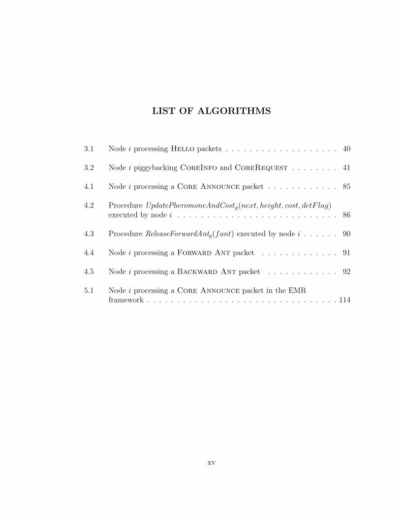
3.1 Node i processing Hello packets . . . . . . . . . . . . . . . . . . . 40
3.2 Node i piggybacking CoreInfo and CoreRequest . . . . . . . . 41
4.1 Node i processing a Core Announce packet . . . . . . . . . . . . 85
4.2 Procedure UpdatePheromoneAndCostg(next, height, cost, detF lag)executed by node i . . . . . . . . . . . . . . . . . . . . . . . . . . . 86
4.3 Procedure ReleaseForwardAntg(fant) executed by node i . . . . . . 90
4.4 Node i processing a Forward Ant packet . . . . . . . . . . . . . 91
4.5 Node i processing a Backward Ant packet . . . . . . . . . . . . 92
5.1 Node i processing a Core Announce packet in the EMRframework . . . . . . . . . . . . . . . . . . . . . . . . . . . . . . . . 114
xv

ABSTRACT
Ad hoc networks consist of (mobile) nodes that autonomously establish con-
nectivity via multihop wireless communications. Without relying on any pre-config-
ured infrastructure or centralized control, ad hoc networks can be instantly deployed
and hence are useful in many situations where impromptu communication facilities
are required. Many applications of ad hoc networks require collaboration of nodes
and expect them to communicate as a group rather than as pairs of individuals.
Hence, multicast is one critical service to support these applications. Providing
multicast functionality over mobile wireless ad hoc networks, however, poses many
challenges due to their unique characteristics. While efficient multicast connectivity
is preferable when resources are scarce, multicast connectivity should also be robust
enough to cope with network dynamics caused by mobility and node failures. Our
research focuses on developing techniques that balance between the efficiency and
the effectiveness of ad hoc multicast routing in various mobility conditions. In this
dissertation, we first introduce the Adaptive Dynamic Backbone Multicast (ADBM)
that utilizes an underlying adaptive distributed clustering algorithm to provide a
mobility-adaptive multicast service. We then describe the MANSI (Multicast for Ad
hoc Network with Swarm Intelligence) protocol, which relies on a swarm intelligence
based optimization technique to learn and discover efficient multicast connectivity.
Simulation study shows that both protocols perform effectively and efficiently in
static or quasi-static environments, yet still effectively in highly dynamic environ-
ments. In addition, we propose the Evolutionary Multicast Routing Framework
(EMRF) for ad hoc networks. EMRF allows us to create a multicast protocol from
xvi
independent incorporation of different mechanisms by dividing the reactive multi-
cast routing process into two phases: initialization and evolution. Using EMRF,
we can design protocol instances that can quickly and efficiently establish initial
multicast connectivity and/or improve the resulting connectivity via different opti-
mization techniques. Finally, we describe our study on the benefits and impacts of
incorporating directional antennas into ad hoc multicast routing protocols.
xvii
Chapter 1
INTRODUCTION
Ad hoc networks consist of (mobile) nodes that autonomously establish con-
nectivity via multihop wireless communications. Without relying on any existing,
pre-configured network infrastructure or centralized control, ad hoc networks can
be instantly deployed, and hence are useful in many situations where impromptu
communication facilities are required. Good examples are battlefield communica-
tions and disaster relief missions, in which communication infrastructures are not
available or have been destroyed. In addition, ad hoc networks can be used in class-
rooms or conferences where participants dynamically share information via their
mobile devices. With this wide range of applications, the typical number of nodes
may range from less than a hundred up to tens of thousands. These characteristics
of ad hoc networks pose unique problems and challenges on their design and opera-
tion. Due to node mobility and wireless communication, the network topology may
change at any time whenever a wireless link is broken or reestablished when a pair
of nodes are moving away from or toward each other, or a node fails or runs out
of power. Bad environmental conditions (e.g., heat, rain) also cause unreliable and
intermittent wireless communication between nodes. In addition, ad hoc networks
are usually deployed in unattended environments, hence their only power sources
are batteries. Furthermore, many nodes are only small devices with limited amount
of memory, storage, and computing power. As a result, communication protocols,
especially routing techniques, as well as other applications and services developed
for this type of networks should be aware of mobility and resource usage.
1
For many applications, nodes need collaboration to achieve common goals
and are expected to communicate as a group rather than as pairs of individuals
(point-to-point). For instance, soldiers roaming in the battlefield may need to hear
a group commander (point-to-multipoint), or a group of commanders may tele-
conference current mission scenarios with one another (multipoint-to-multipoint).
Therefore, multipoint communications become more widespread and serve as one
critical operation to support these applications. Similar to multicast protocols for
wired networks such as IP multicast [KR00], one of the major goals in designing
multicast protocols for ad hoc networks is to reduce unnecessary packet delivery
to other nodes outside the group by having only a subset of nodes participating in
multicast data forwarding. However, due to the peculiarities of ad hoc networks,
traditional IP multicast techniques are unsuitable, and a new paradigm for ad hoc
multicast routing is required.
Multicast Routing Problem in Ad hoc Networks
In traditional static IP networks, the goal of multicast routing is to find a tree
of links connecting all routers that belong to a certain multicast group. How-
ever, IP multicast protocols [BFC93, DEF+96, DC90, Moy94] are inappropriate
for ad hoc networks because multicast trees could easily break due to dynamic
topologies [LSH+00]. Many multicast protocols for ad hoc networks have been pro-
posed. Some protocols still rely on constructing a tree spanning all group members
[LTM99, WT99], which is not robust enough when the network becomes more dy-
namic with less reliable wireless links. In contrast, many proposed protocols have
data packets transmitted into more than one link, and allow packets to be received
on links that are not branches of a multicast tree. These protocols fall into a cate-
gory of mesh-based protocols in that group connectivity is formed as a mesh rather
than a tree to increase robustness at the price of adding more redundancy in data
transmission. Flooding, where data packets are forwarded to and received from all
2
�����������
������ �������� ��
�����������
�����������
������ �� �����������
(a) (b)
Figure 1.1: Multicast operations with directional antennas: (a) Multicast packets
directionally sent to multiple members in the same sector, allowing
another source to transmit a packet simultaneously, and (b) Multicast
packet sent to multiple members located in different sectors
links, is also considered a mesh protocol since the mesh is in fact the entire network
topology. In highly dynamic, highly mobile ad hoc networks, a flooding approach
is a better alternative to multicast routing due to its minimal state maintained and
high reliability [HOTV99]. As the extreme, flooding provides the most robust, but
inefficient mechanism since a multicast packet will be forwarded to every node (as
long as the network is not partitioned), while a tree-based approach offers efficiency
but is not robust enough to be used in highly dynamic environments. Furthermore,
routing based on a connected dominating set [KKRM01, SSB99a, SSB99b, SDB98]
can also increase the overall efficiency since the search space is reduced to only nodes
in the dominating set during route discovery and maintenance processes.
Multicast Communications with Directional Antennas
Research in ad hoc networks has been primarily focused on networking issues assum-
ing the use of omni-directional antennas with collision avoidance medium access con-
trol protocols such as IEEE 802.11. Although a variety of directional antenna-based
3
local multicast tree branch
backbone connectivity
multicast group member
normal node
backbone node (core)
local tree maintenance
static highly dynamic
flooding
Figure 1.2: Adaptability of multicast inherited from the adaptive backbone con-
struction mechanism: more backbone nodes appear in a more dynamic
area than the others of the network, causing a shift of the forwarding
mechanism from tree-based forwarding to flooding in that area
MAC protocols have been proposed [HS02, HSSJ02a, KSV00, NYH00, SGZ01], there
lack suitable mechanisms to fully exploit the provided capabilities through knowl-
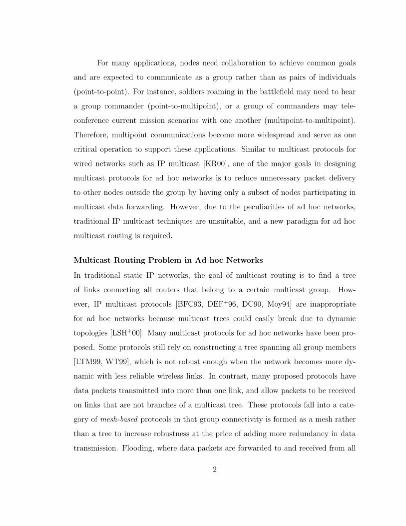
edge from other layers such as the network layer. For example, an expected group of
receivers, along with their direction information, could be supplied from the network
layer so that broadcast and multicast communication would be efficiently performed,
as shown in Figure 1.1.
Research Objectives
This research work has two main objectives. The first objective is to develop adap-
tive, scalable and mobility-aware multicast techniques for ad hoc networks. Al-
though several ad hoc multicast protocols have been proposed in the literature,
most of them rely on different approaches based on different assumptions about the
environments, hence they are only suitable for networks under specific conditions.
Our techniques are designed to combine the effectiveness of a flooding scheme and
the efficiency of the tree-based approach to support a wide range of operational
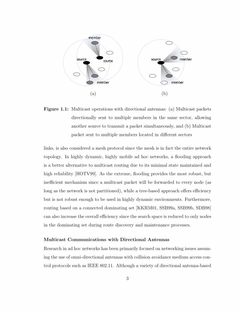
configurations, even within the same network. For example, Figure 1.2 illustrates a
4

BA
C
BA
C
(a) (b)
Figure 1.3: Examples of multicast connectivity among three group members (black
circles): (a) six other nodes, shown in gray, establishing group con-
nectivity and participating in multicast data forwarding, and (b) more
efficient data forwarding when there are only four nodes forming group
connectivity
network with two different portions in terms of mobility speed. The left portion of
the network is relatively static, while nodes on the right side move with higher speed.
When there is low mobility in the network, the multicast operation should behave
using a tree-based protocol to take advantage of the efficiency of the multicast tree
structure. On the contrary, a multicast tree is difficult to be efficiently maintained
over fast-moving nodes, hence operations that resemble partial flooding would be
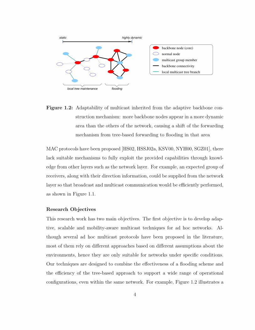
more effective. In addition, we also adapt the swarm intelligence metaphor [BDT99]
to develop a multicast routing protocol that allows more efficient group connectivity
to be learned (or discovered) over time. For instance, a multicast connection linking
three members can be quickly established with low efficiency (e.g., resulting in a
relatively large number of nodes participating in data forwarding), as illustrated in
Figure 1.3(a). Later in time, nodes begin to change their roles and evolve into a
new and smaller forwarding set (Figure 1.3(b)), which is more efficient in terms of
data forwarding. By abstracting the cost associated with each forwarding node, we
5

discuss that this technique can be applied to different variations of the multicast
routing problem by representing the cost with different measurements.
The other objective of our research is to develop methods to incorporate di-
rectional antennas into multicast communications in ad hoc networks and investigate
their benefits and impacts on application performance.
Accomplishments and Contributions: Structure of the Dissertation
Throughout this dissertation, we elaborate our accomplishments which address the
aforementioned research objectives. We have
• Surveyed literature on multicast for ad hoc networks, including background
on swarm intelligence and directional antennas. [Chapter 2]
• Developed a distributed clustering algorithm, called Adaptive Dynamic Back-
bone [JS02] or ADB for short, which creates a virtual backbone infrastruc-
ture to facilitate mobility-adaptive multicast routing. Various techniques to
increase efficiency of multicast communications were developed and studied.
[Chapter 3]
• Designed a multicast routing protocol based on the swarm intelligence metaphor,
called MANSI (Multicast for Ad hoc Networks with Swarm Intelligence) [SJ],
which allows multicast connections of lower total (abstract) costs to be learned
(or discovered) over time. [Chapter 4]
• Introduced a framework for evolutionary multicast routing for ad hoc networks.
The framework allows independent incorporation of different mechanisms for
initializing and optimizing multicast connectivity. This incorporation there-
fore creates protocol instances that can quickly and efficiently establish initial
multicast connectivity and/or effectively improve the resulting connectivity
via different optimization techniques. As an instance of the framework, we
6
combined ADB and the swarm intelligence based technique used by MANSI
into one single protocol and studied its behavior and performance. [Chapter 5]
• Implemented simulation models for the above protocols and studied their per-
formance in several aspects, such as multicast group size, mobility speed, and
traffic load. [Chapters 3, 4 and 5]
• Studied the benefits and impacts of multicast communications under different
operation modes of switched-beam directional antennas, both analytically and
experimentally [JS03]. [Chapter 6]
7
Chapter 2
BACKGROUND AND RELATED WORK
In this chapter, we review existing multicast routing protocols for ad hoc
networks. These protocols are classified based on how they employ intermediate
nodes to relay multicast data packets from sources to other group members (a tax-
onomy based on connectivity). We also describe other taxonomies. In addition, we
review background information of swarm intelligence and wireless communication
with directional antennas, which are fundamental knowledge we have adopted in
this research.
2.1 Multicast Techniques for Mobile Ad hoc Networks
To provide multicast routing over mobile ad hoc networks, the challenge is
to effectively handle frequent topology changes caused by node mobility/failure and
link disruption due to interference and jamming. A number of multicast techniques
have been proposed to address this issue. These protocols are ranging from a simple
flooding scheme to state-based tree or mesh structures, as well as hierarchical and hy-
brid approaches. Based on their operations, there exist different taxonomy schemes
to classify these ad hoc multicast routing protocols, including connectivity among
group members (tree-based vs mesh-based), route acquisition schemes (proactive vs
reactive), connectivity initialization (sender-initiated vs receiver-initiated), depen-
dency on unicast routing, and forwarding state maintenance schemes (source-based
vs group-shared).
8

2.1.1 Taxonomy Based on Connectivity
In this section, we classify ad hoc multicast protocols based on the method-
ologies used to maintain connectivity among group members. Other classification
schemes will be described in Section 2.1.3.
2.1.1.1 Tree-based Protocols
In static networks like traditional IP networks, tree-based multicast protocols
are efficient in terms of bandwidth consumption, and hence are often preferred. Some
proposed techniques have adopted the traditional tree-based IP multicast scheme,
while others employ different techniques to create and maintain tree structures for
efficiency. However, with the dynamic nature of ad hoc networks, attempting to
maintain a valid tree all the time might end up consuming significant amount of
network bandwidth due to frequent topology changes.
AMRoute (Ad hoc Multicast Routing Protocol) [LTM99] is based on the IP
multicast concept. To cope with dynamics in the network, the protocol only keeps
track of the group members and lets member nodes communicate with each other via
IP-in-IP tunnels in the same way as connecting multicast routers in MBone [Eri94].
Consequently, AMRoute relies on an underlying unicast routing protocol which is
responsible for taking care of topology changes. Multicast states are only main-
tained by group members, as a group-shared tree is created and maintained among
them. This also means that other non-member nodes are not required to support IP
multicast. Since the protocol is not aware of nodal mobility (as it relies on a unicast
routing protocol to connect member nodes), the multicast tree is suboptimal and
may potentially cause temporary routing loops when nodes are moving.
Many tree-based protocols are designed to be tightly coupled with their
base unicast routing protocols to provide multicast support with minimum addi-
tional overhead. For instance, LAM (Lightweight Adaptive Multicast) [JC98] is a
9
tree-based multicast protocol that is tightly coupled with TORA (Temporally Or-
dered Routing Algorithm) [PC01]. LAM creates a group-shared tree for each group
rooted at a pre-selected core node (similar to the Core-Based Tree (CBT) proto-
col [BFC93]). Since TORA already provides a mechanism to create a destination-
oriented DAG (Directed Acyclic Graph) for each possible destination in the network,
a node willing to join a multicast group makes use of a DAG with respect to the
core to connect to the multicast tree. Any changes in topology are handled trans-
parently by TORA as well. Another example is the MAODV (Multicast Ad Hoc
On-Demand Distance Vector) protocol [RP99], which is a multicast extension of the
AODV (Ad hoc On-demand Distance Vector) routing protocol [PRD01]. AODV and
its multicast extension MAODV together are therefore considered a single routing
protocol that supports both unicast and multicast routing. The protocol creates a
multicast tree per group rooted at the first member of the group, called the group
leader. Unlike LAM, group leadership in MAODV can be dynamically assigned dur-
ing multicast sessions. It also incorporates a sophisticated mechanism that allows
multicast connectivity to be maintained even when the network gets partitioned by
assigning a new group leader for each partition that gets separated from the main
network. When two partitions rejoin, the two trees then merge and only one group
leader continues to serve as the group leader for the reconnected tree.
In contrast, AMRIS (Ad hoc Multicast Routing with Increasing id-numberS)
[WT99] is a tree-based protocol that does not rely on any underlying unicast routing
protocol. For each multicast group, it creates a group-shared tree rooted at a special
node, called Sid, which is the sender node (in case of single sender) or is elected from
the set of senders. Each node participating in a multicast session is assigned an id,
called msm-id (multicast session member id). The msm-id’s are increasing as nodes
are located further away from the Sid. The use of msm-id’s is to avoid routing loops
created during a link recovery since only the child node (i.e., the node with the
10

higher msm-id of the broken link) is allowed to initiate the reconstruction process.
There are a number of tree-based multicast protocols that take into account
mobility levels or stability of nodes or paths, and adapt their mechanisms accord-
ingly. One of these protocols is the adaptive shared tree multicast [CGZ98a]. It is an
integration of a source-based tree approach and a group-shared tree approach. With
a two-level mobility model, nodes are classified into two categories, slow-moving
nodes and fast-moving nodes. A multicast tree is initially created as a group-shared
tree where the root is selected from the group of slow-moving nodes. A source may
switch to use a source-based tree instead when the source observes that it is a slow
node because a source-based tree would be more efficient in terms of delays and
packet transmissions. In addition, when a receiver node notices that a multicast
packet took a much longer path through the root (core) than it would if it were sent
directly from the source, the receiver node will explicitly ask the source to switch
to the source-based mode only for this source/receiver pair. ABAM (Associativity-
Based Ad hoc Multicast) [TGB00] is yet another example which attempts to main-
tain stable source-based multicast trees. Its criteria for selecting a tree branch are
different from those of other multicast protocols described above in that, in addition
to the number of hops, association stability such as spatial, temporal, connection
and power stability of nodes with their neighbors along the path is also considered.
2.1.1.2 Mesh-based Protocols
Although a tree structure can support efficient multicast operations in gen-
eral, it can be very fragile in dynamic environments where links can break due to
node mobility or link failure since there is only one path connecting a source to a
receiver [LSH+00]. Furthermore, many tree-based protocols that are based on the
reverse path forwarding technique or the core-based tree often require shortest path
information from unicast routing tables to operate. Initialization and maintenance
11

B
A
D E
C
G
FB
A
D E
C
G
FB
A
D E
C
G
F
(a) (b) (c)
Figure 2.1: Examples of multicast connectivity in tree-based and mesh-based ap-
proaches (solid lines denote paths on which multicast packets are for-
warded, and nodes in shade denote multicast group members): (a) a
multicast tree, (b) a multicast mesh, and (c) a multicast full mesh
(flooding)
overhead will increase significantly in mobile ad hoc environments since they usu-
ally employ on-demand routing protocols, which normally do not maintain complete
routing tables. Furthermore, using proactive routing protocols or trying to keep the
routing tables updated all the time is not desirable due to an unacceptable amount
of control traffic.
To provide path redundancy, several ad hoc multicast protocols based on a
mesh structure have been proposed. Unlike a tree, data packets are allowed to be
forwarded to the same destination through more than one path, which increases
chances of successful delivery. Figure 2.1 illustrates this situation. If the link be-
tween the receiver A and the source C is broken, with a tree-based approach in
Figure 2.1(a), A will not be able to receive data from C. In contrast, the link
breakage will not prevent A from receiving data with a mesh structure shown in
Figure 2.1(b), since D is serving as a backup path between A and C.
FGMP (Forwarding Group Multicast Protocol) [CGZ98b] and ODMRP (On
Demand Multicast Routing Protocol) [BLSG00] maintain a mesh on top of a group
12
of nodes known as a forwarding group. In FGMP, construction of a forwarding
group is initiated by either a sender or a receiver flooding a request, depending on
whether the sender advertising mode (FGMP-SA) or the receiver advertising mode
(FGMP-RA) is used. In situations where the number of senders is less than the
number of receivers, FGMP-SA is preferable. Each node in a forwarding group
sets a forwarding flag which is associated with a soft-state timer and periodically
refreshed by the sender (in FGMP-RA) or the receiver (in FGMP-SA). To correctly
identify the next hop on the shortest path back to a sender or a receiver, FGMP
requires the existence of routing tables from an underlying unicast routing protocol.
ODMRP is similar to FGMP-SA except that a forwarding group is established and
updated by a sender on demand (i.e., as long as it has data to send), while in FGMP,
the sender periodically floods its membership all the time. Because each node also
keeps track of the previous node back to the sender while it is receiving the sender’s
request, ODMRP requires no unicast routing protocol to operate.
To maintain a multicast forwarding group in ODMRP, the senders period-
ically flood the network with join request messages when they have data sent to
the group. Although the protocol yields a high packet delivery ratio even at high
mobility [LSH+00], doing so can cause excessive overhead and lead to scalability
problem in larger networks and/or with large number of senders. NSMP (Neigh-
bor Supporting Ad hoc Multicast Routing Protocol) [LK00] takes another approach
to minimizing the amount of broadcast control messages during the maintenance
process by limiting the propagation of control messages to only forwarding nodes
and their neighbor nodes. As a result, any node within two hops away from the
mesh can provide a point of attachment for a migrated receiver node. However,
control message flooding is still used during the initialization process and the recov-
ery process of a receiver with more than two hops away from the mesh. A different
approach to reducing excessive packet flooding is utilized by DCMP (Dynamic Core
13
based Multicast routing Protocol) [DMM02]. In DCMP, not all group senders are
required to flood join requests periodically. Instead, senders are classified into ac-
tive senders, core active senders and passive senders. Active senders are responsible
for maintaining the mesh by flooding join requests periodically, similar to senders
in ODMRP, while passive senders rely on their nearby active senders to flood join
requests on their behalfs.
Under very high mobility, any multicast protocol that relies on states main-
tained by each node cannot efficiently keep the states valid long enough, which fre-
quently results in inconsistency in the network that, in turn, causes unreliability in
unicast and multicast communication. In such scenarios, flooding [HOTV99], being
stateless and topology-independent, becomes more appropriate. However, previous
experimental results show that flooding can still become unreliable under extremely
high mobility speed.
All of the above mesh-based approaches rely on network-wide flooding to
some degree, which could bring about a scalability problem for large networks.
There are different approaches to avoiding global flooding. One approach is to
use an expanding-ring search technique which starts with a small flooding scope
and extends the scope if the last step fails. The bandwidth-efficient multicast pro-
tocol [OKS01] employs this technique during its route setup and route recovery
processes. CAMP (Core-Assisted Mesh Protocol) [GLAM99] avoids control mes-
sage flooding by relying on rendezvous points [BFC93], so that control messages are
directed to a core, if available, instead of being flooded to the entire network. When
a core is unavailable or unreachable, an expanding-ring search is used. CAMP also
supports the simplex mode which gives an efficient way for sender-only nodes to join
the mesh. By this means, data packets are sent in only one direction from the senders
to the mesh but not the other way around. CAMP relies on an underlying unicast
routing protocol which provides correct distances to known destinations within a
14
finite time to achieve minimal delays by ensuring that shortest paths from receivers
back to sources are part of the group’s mesh. A heartbeat message is periodically
sent out by each source and is retransmitted by forwarding nodes if the message is
received from a node that is on the shortest path back to the source. If a member
detects that the neighbor on the shortest path to the source is not yet part of the
mesh, that member sends a push join to that neighbor to ask it to become part
of the mesh. Several other protocols exploit the concept of connected backbones
or connected dominating sets to avoid network-wide flooding. These protocols are
described in Section 2.1.2.
2.1.2 Hierarchical, Hybrid and Adaptive Protocols
This section covers ad hoc multicast protocols that view the network as be-
ing hierarchical rather than flat, including adaptive protocols that are not strict
to one specific scheme (i.e., tree or mesh), but adapt their behaviors to different
environment conditions. To achieve scalability, a hierarchical approach or a hybrid
approach is often employed.
MZR (Multicast Zone Routing Protocol) [DS01] adopts a hybrid approach
using the same mechanism provided by the Zone Routing Protocol (ZRP) [HP97]. A
zone is defined for each node with a radius representing the number of hops from the
node. A proactive, or table-driven, protocol is used inside each zone, while reactive
route queries are carried on at the zone border nodes on demand, resulting in a
much smaller number of nodes participating in the global flooding search. The zone
size is fixed for every node and for the entire operation of the network. Previous
study [HP99] has shown that the optimal zone radius for the zone routing protocol
is two.
Another approach to reducing the number of participants when a global flood-
ing is needed is based on the notion of connected dominating sets. This approach is
exploited by CGM (Clustered Group Multicast) [LC99], and MCEDAR (Multicast
15
Core-Extraction Distributed Ad hoc Routing) [SSB99b] which is an extension to
the CEDAR [SSB99a] unicast routing architecture. A set of nodes, called a domi-
nating set, are extracted from the network through clustering, backbone construc-
tion, or minimum connected dominating set algorithms [BGLA03, Bas99, BTD01,
KKRM01, SDB98]. Once a dominating set is obtained, any node must either belong
to the set or be an immediate (one-hop) neighbor of a node in the set. These nodes
then form a virtual backbone which may be used to carry both multicast data and
control traffic as in CGM, or control traffic only as in MCEDAR.
Most ad hoc multicast protocols propose different approaches based on differ-
ent assumptions about the environments such as mobility speeds. Several adaptive
multicast protocols have been proposed to incorporate different behaviors within
the same protocol. An adaptive protocol for reliable multicast [GS99b] utilizes a
combination of a tree-based mechanism and a flooding mechanism to achieve adapt-
ability of multicast operation in various mobility speeds. By default, in a static
environment, the protocol creates a core-based tree for each group to connect all
the multicast group members. In addition, each tree node u is associated with a for-
warding region defined as the maximal subgraph of non-tree nodes around u. With
mobility, nodes that witness a topology change will flood multicast packets over their
forwarding regions which glue the fragments of the multicast tree together. This
means that a packet will always be flooded to all the forwarding regions associated
with nodes that witness a topology change, while other nodes whose neighbor lists
remain unchanged still use an existing multicast tree for data forwarding. This pro-
tocol also employs an acknowledgment-based mechanism to guarantee reliability in
delivery of multicast data. ADMR (Adaptive Demand-Driven Multicast Routing)
[JJ01] is another source-based, on-demand multicast protocol that has the capa-
bility to switch to the flooding mode when receivers detect high mobility in their
areas, and turn back to normal operation after some period of time. By combining
16
Adaptive Techniques
FGMP [CGZ98b]CAMP [GLAM99]Bandwidth-efficient [OKS99]Flooding [HOTV99]NSMP [LK00]ODMRP [BLSG00]DCMP [DMM02]MANSI [SJ]CGM [LC99]MCEDAR [SSB99b]ADBM [JS02]
Multicast Techniques
Tree-basedTechniques
Mesh-basedTechniques
Reliable Mcast [GS99b]
AMRIS [WT99]ABAM [TGB00]AMRoute [LTM99]MAODV [RP99]Adaptive Shared Tree [CGZ98a]LAM [JC98]
ADMR [JJ01]CGM [LC99]MCEDAR [SSB99b]ADBM [JS02]
MZR [DS01]MZR [DS01]
Hierarchical/Hybrid/
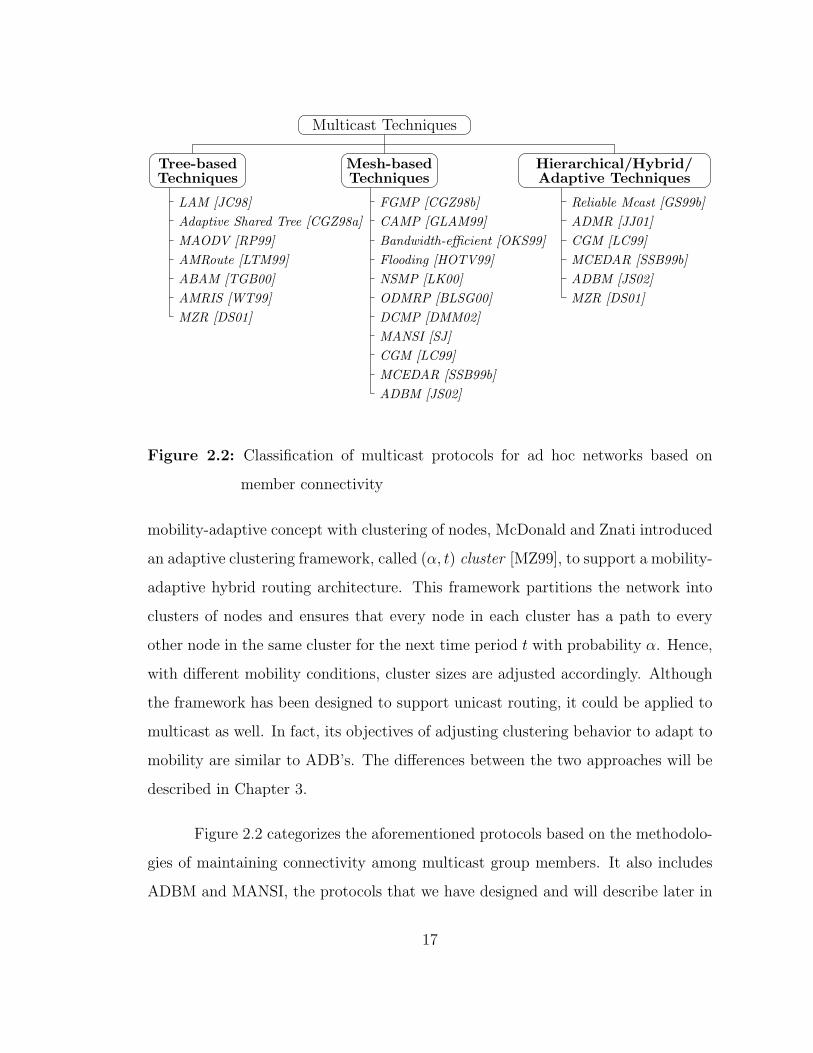
Figure 2.2: Classification of multicast protocols for ad hoc networks based on
member connectivity
mobility-adaptive concept with clustering of nodes, McDonald and Znati introduced
an adaptive clustering framework, called (α, t) cluster [MZ99], to support a mobility-
adaptive hybrid routing architecture. This framework partitions the network into
clusters of nodes and ensures that every node in each cluster has a path to every
other node in the same cluster for the next time period t with probability α. Hence,
with different mobility conditions, cluster sizes are adjusted accordingly. Although
the framework has been designed to support unicast routing, it could be applied to
multicast as well. In fact, its objectives of adjusting clustering behavior to adapt to
mobility are similar to ADB’s. The differences between the two approaches will be
described in Chapter 3.
Figure 2.2 categorizes the aforementioned protocols based on the methodolo-
gies of maintaining connectivity among multicast group members. It also includes
ADBM and MANSI, the protocols that we have designed and will describe later in
17
Chapter 3 and Chapter 4, respectively.
2.1.3 Other Classifications for Multicast Protocols
The classification described in the previous section is based on how multicast
connectivity is set up (i.e., a tree vs a mesh). In fact there are other many different
aspects we can consider for protocol classification, which include, but are not limited
to, the following:
• Proactive vs reactive
Similar to unicast routing protocols, multicast routing protocols can also be
classified as either proactive or reactive. A protocol is considered proactive
if it continuously maintains multicast connectivity (i.e., tree/mesh) among
group members, regardless of the availability of data traffic. This scheme is
advantageous in that the multicast connectivity is readily available for data
transfer. However, it may often end up using a large portion of valuable
network bandwidth to keep the connectivity updated, especially when the
network topology is dynamic. Therefore, a proactive scheme is usually suitable
for networks with low mobility.
In contrast, reactive protocols attempt to establish connectivity among mem-
bers on demand, i.e., only when a source has data to send. Therefore, no
bandwidth is wasted even though the network topology keeps changing, given
that nobody has data to send. A drawback of a reactive scheme is the longer
multicast route acquisition time and frequent use of network-wide flooding.
• Sender-initiated vs receiver-initiated
This aspect concerns how multicast tree or mesh formation is initialized. The
establishment of multicast connectivity can be initiated by multicast sources,
receivers, or both. In a sender-initiated protocol, each source is responsible
18

for announcing its own existence to other nodes in the network so that nodes
who are members can reply with join messages, resulting in establishment
of group connectivity. The announcement can be done periodically or on
demand. A receiver-initiated protocol, in contrast, requires each receiver to
initiate a request to the group by searching for a point of attachment to the
current tree/mesh, or sending a direct request to a special node such as the
rendezvous point or the core. Source nodes, which may not be part of the
group connectivity, then send data packets to the core so that data can be
distributed to the group receivers.
In some protocols, both sources and receivers have no clear distinction and are
treated equally as group members. Generally, these protocols exploit similar
mechanisms used by receiver-initiated protocols. The first node who joins the
group may become the group leader and serve as a focal point for other group
members to establish connectivity.
Notice that a reactive protocol is often a sender-initiated protocol as well due
to the fact that connectivity is established upon availability of the multicast
data, which is first known by multicast sources.
• Unicast-dependent vs unicast-independent
As stated earlier, certain multicast protocols rely on underlying unicast pro-
tocols to operate, while many others have been designed to operate indepen-
dently. Since achieving certain tasks with unicast routing may end up with
unnecessary operations and waste of bandwidth, designing a multicast pro-
tocol to be independent of any unicast protocol allows the protocol to have
complete knowledge about and better utilize the control overhead. On the
contrary, tying a multicast protocol to unicast routing can also be beneficial.
19
For instance, protocols that are tightly coupled with their base unicast rout-
ing protocols are able to exploit routing information and provide multicast
capability with minimum additional overhead due to elimination of redun-
dant tasks. Some protocols employ unicast routing functionality as a low-level
mechanism to logically connect group members together, making the multicast
mechanism itself independent to the network dynamics.
• Source-based vs Group-shared Connectivity
A multicast tree or mesh may be created and used to forward data packets
generated by a particular source (source-based connectivity), or by any source
within the group (group-shared connectivity). A source-based tree/mesh is
often created as a combination of shortest paths from the receivers to the
corresponding source, thus giving a major advantage in that end-to-end delays
are minimum. In addition, having different sources employ different groups
of nodes to forward data packets also helps in terms of traffic load balancing.
However, having each source maintain its own connectivity separately can
potentially yield more control overhead. For intermediate nodes, separate
forwarding states are required for each source as well. Therefore, this scheme
is suitable for networks with smaller number of sources, and for applications
whose delays are critical.
Creating a single tree/mesh per group allows nodes to become multicast sources
and to send data to the group by sharing the existing connectivity. This scheme
is therefore suitable in situations where each member can be a sender, a re-
ceiver, or both at any time. One drawback is higher traffic concentration on
certain nodes due to the shared connectivity, which may result in congestion
when sources generate heavy traffic load. The selection of the node who will
serve as a focal point for establishing (optimal) connectivity for the entire
group is also a critical issue.
20
Table
2.1
:Sum
mar
yof
exis
ting
mult
icas
tte
chniq
ues
for
adhoc
net
wor
ks
Techniq
ue
/P
roto
col
connectivity
route
acquis
itio
nin
itia
lizati
on
unic
ast
dependent
state
main
tain
ed
contr
olm
ess
age
floodin
g
AB
AM
[TG
B00]
tree
react
ive
sourc
eno
per
-sourc
eyes
Adaptive
share
dtr
ee[C
GZ98a]
tree
pro
act
ive
both
yes
per
-gro
up/per
-sourc
eno
AM
RIS
[WT
99]
tree
react
ive
elec
ted
sourc
eno
per
-gro
up
yes
AM
Route
[LT
M99]
tree
pro
act
ive
both
yes
per
-gro
up
yes
Bandw
idth
-effi
cien
t[O
KS99]
mes
hpro
act
ive
both
no
per
-gro
up
yes
CA
MP
[GLA
M99]
mes
hpro
act
ive
both
yes
per
-gro
up
no
CG
M[L
C99]
mes
hre
act
ive
both
no
per
-gro
up
no
DC
MP
[DM
M02]
mes
hre
act
ive
sourc
eno
per
-gro
up
yes
FG
MP
-RA
[CG
Z98b]
mes
hpro
act
ive
rece
iver
yes
per
-rec
eiver
yes
FG
MP
-SA
[CG
Z98b]
mes
hpro
act
ive
sourc
eyes
per
-sourc
eyes
Flo
odin
g[H
OT
V99]
mes
hre
act
ive
sourc
eno
none
no
LA
M[J
C98]
tree
pro
act
ive
both
yes
per
-gro
up
no
MA
OD
V[R
P99]
tree
pro
act
ive
both
yes
per
-gro
up
yes
MC
ED
AR
[SSB
99b]
mes
hre
act
ive
both
no
per
-gro
up
no
MZR
[DS01]
tree
hybri
dso
urc
eno
per
-sourc
eno
NSM
P[L
K00]
mes
hre
act
ive
sourc
eno
per
-gro
up
yes
OD
MR
P[B
LSG
00]
mes
hre
act
ive
sourc
eno
per
-gro
up
yes
Rel
iable
mca
st[G
S99b]
tree
/m
esh
pro
act
ive
both
yes
per
-gro
up
no
AD
MR
[JJ01]
mes
hpro
act
ive
both
no
per
-sourc
eyes
AD
BM
[JS02]
mes
hpro
act
ive
both
no
per
-gro
up
no
MA
NSI
[SJ]
mes
hre
act
ive
firs
tso
urc
eno
per
-gro
up
yes
21
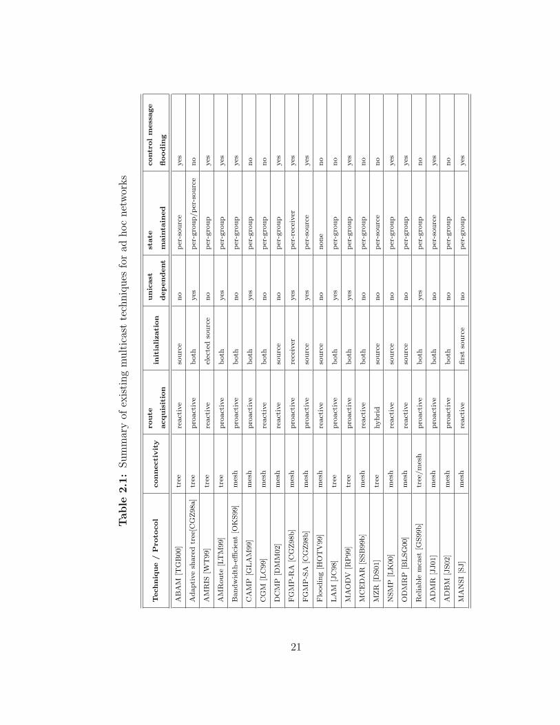
Table 2.1 summarizes the characteristics of existing ad hoc multicast proto-
cols with respect to all the above aspects. The protocols ADBM and MANSI are
incorporated in the table as well.
2.2 Biologically Inspired Algorithms for Computer Networks
Swarm intelligence [BDT99] appears in biological swarms of certain insect
species such as ants and honeybees. Although each individual (for instance, an ant)
has little intelligence and follows simple rules using local information obtained from
the environment, globally optimized objectives1 emerge when they work collectively
as a group. Inspired by this behavior, swarm intelligence metaphor has been applied
to many combinatorial optimization problems such as the traveling salesman prob-
lem (TSP) and the quadratic assignment problem (QAP) [DMC96, DCG99]. In com-
munications networks, a number of routing and load balancing mechanisms based
on swarm intelligence have been proposed. Ant-Based Control (ABC) [SHBR96] ap-
plies swarm intelligence to achieve load balancing in telecommunications networks.
Simulated on a model of the British Telecom (BT) telephone network, ABC has
been shown to result in fewer call failures than other methods such as shortest-path
routing. In [CD97, CD98], a distributed adaptive routing for datagram networks,
called AntNet, is described. Although several variations of AntNet have been de-
veloped, all of them rely on the same concept where forward ants are launched
toward destinations while probing path quality along the way, and backward ants
travel back and update pheromone on the backward paths. The amount of added
pheromone is proportional to the goodness of the path measured by the forward
ants.
Swarm intelligence has also been extended to multicast routing problem. Das
1 A common example is that ants often find a shortest path from their nest tothe food source
22
et al. [DGHV02] proposed an ant-based heuristic to solve the Steiner tree problem—
finding minimum-cost trees that span a subset of network nodes (e.g., multicast
group members)—which is known to be NP-complete. The algorithm produces
near-optimal to optimal results for test runs. Chu et al. [CGHG02] applied an ant
colony approach to the QoS multicast routing (QMR) problem, defined as find-
ing the minimum-cost path from the source to all the destinations while meeting
all QoS constraints. The algorithm has been shown to find optimal (or near opti-
mal) solutions quickly with good scalability. Both algorithms, however, require the
global knowledge of the network topology, and hence are not suitable for dynamic
environments, such as mobile ad hoc networks. Lu et al. [LLZ00] introduced a dis-
tributed multicast routing scheme, using an ant algorithm, for delay-bounded and
load-balancing traffic. The scheme is similar to AntNet in that a source deploys for-
ward ants to each of the multicast group members, which, in turn, return backward
ants back to the source and learn routes with low delays and less congestion. Sources
are assumed to have knowledge of all the group members from the beginning.
The concept of swarm intelligence has recently been applied to solve various
problems in the ad hoc network domain. Camara and Loureiro adopted ant-like
mobile software agents to collect and disseminate the information about nodes’
GPS locations in the routing algorithm, called GPSAL (GPS/Ant-Like Routing
Algorithm) [CL00a, CL00b]. Kassabalidis et al. proposed the Adaptive Swarm-based
Distributed Routing (Adaptive-SDR) [KESI+02] for routing in wireless and satellite
networks. It incorporates a mechanism to cluster nodes into colonies to resolve
the scalability issue in large networks. Heissenbuttel and Braun [HB03] exploited
a different approach to routing in large scale ad hoc networks by grouping nodes
into logical routers based on their geographical locations. An ant-based routing
algorithm is then performed on top of this logical topology.
All the above ant-based routing algorithms for ad hoc networks are proactive,
23
as ants are periodically deployed to collect information from the beginning. In con-
trast, Gunes et al. adopted an on-demand approach to ant-based ad hoc routing and
introduced the Ant-colony-based Routing Algorithm (ARA) [GSB01, GS02]. Simi-
lar to other on-demand routing protocols such as AODV [PRD01] and DSR [JM01],
ARA floods a forward ant as a route discovery packet to find a destination, where a
backward ant is sent back as a route reply. However, a backward ant not only comes
back on the reverse path, but is also flooded to establish the pheromone trails back
to the destination (as the forward ant does for the source). A hybrid routing proto-
col that combines ant-based routing and AODV has been proposed by Marwaha et
al. as an attempt to reduce route discovery latency in pure AODV, and route conver-
gence time in pure ant-based routing. This protocol, called Ant-AODV [MTS02],
exploits AODV’s on-demand route discovery mechanism to find unknown routes,
while deploying ants independently to obtain other routes in advance.
As part of our research, we adapt swarm intelligence to develop an on-
demand, mesh-based multicast protocol for mobile ad hoc networks, called MANSI
(Multicast for Ad hoc Networks with Swarm Intelligence), which focuses on reduc-
ing overall cost of the mesh. MANSI will be described in details in Chapter 4. To
our knowledge, no multicast protocols for ad hoc networks exploiting the concept
of swarm intelligence have been proposed so far.
2.3 Wireless Communication with Directional Antennas
Previous research has already shown significant performance improvement
when directional antennas are used in ad hoc networks. In [NYH00], a new MAC
scheme was proposed to facilitate networking of mobile wireless terminals equipped
24
with directional antennas. The scheme is based on IEEE 802.11 where the transmit-
ting node and the receiving node reserve the channel by omni-directionally broad-
casting RTS (Request-To-Send) and CTS (Clear-To-Send) frames before communi-
cating the data frame. Unlike IEEE 802.11, the data frame is transmitted direction-
ally since the sender has learned the receiver’s direction through the reception of
the CTS frame. However, by using omni-directional RTS frames, the channel may
still not be fully utilized due to the exposed terminal problem. Two other MAC
schemes for directional antennas proposed by Ko et al. [KSV00] work around this
problem by allowing nodes to transmit RTS frames directionally. In case of a node
hearing a RTS or a CTS that is not for itself from one direction, only that direction
is blocked and the other directions are considered available, so that the node does
not have to wait if it has data to send to a direction other than the blocked one.
Since the direction to a receiver has to be known a priori to transmit a directional
RTS, the protocols rely on the availability of a location service such as GPS and
beacon messaging.
While the majority of the directional-antenna-related projects focus on de-
veloping new MAC schemes to fully exploit this type of antennas in unicast com-
munication, little work has been done to extend the support to other layers when
the MAC layer is only used to perform broadcast communication. Nasipuri et al.
[NMMH00] proposed the use of directional antennas for on-demand routing proto-
cols in ad hoc networks to efficiently perform a route discovery by flooding a query
message to a certain direction, instead of flooding them to the entire network. In
contrast, our main focus is to develop techniques and study their performance when
applying directional antennas to multicast communication.
2.4 Summary
In this chapter, we have reviewed related work on multicast techniques for ad
hoc networks. We classified these schemes based on methodologies used for group
25

connectivity (i.e., tree vs mesh), and also pointed out advantages and disadvantages
of each category. We also described taxonomies based on other protocol aspects.
Although several protocols have been proposed, they may be suitable under specific
network conditions, and exhibit drawbacks in other conditions. For instance, some
protocols which are quite aggressive in data forwarding and yield high delivery ratio
in highly dynamic environments can be overkill when the network is relatively static.
As a result, we have developed techniques that offer efficient multicast operations
in static or quasi-static environments, and become more aggressive and effective in
highly dynamic environments, even within the same network.
We also looked into applications of swarm intelligence to computer networks,
especially on routing for ad hoc networks. While there are a number of ant-based
techniques proposed for ad hoc unicast routing, there lacks research and study on
applying swarm intelligence to ad hoc multicast. We believe that swarm intelli-
gence possesses many useful properties which can be beneficial for such dynamic
environments and should be further explored for multicast communication as well.
At the end we presented a survey on applying directional antennas to commu-
nications in ad hoc networks. As previous research has focused mostly on exploiting
directional antennas at physical and MAC layers, we aim to extend the support to
the network layer to which directional information for next hops on the tree/mesh
can be provided.
26

Chapter 3
ADAPTIVE DYNAMIC BACKBONE MULTICAST
Most ad hoc multicast routing protocols reviewed in Chapter 2 are suitable
under specific network conditions, and exhibit drawbacks in others. To provide mul-
ticast routing support for a wide range of operational conditions, even within the
same network, especially in terms of mobility, we have developed a protocol that
integrates the effectiveness of a flooding scheme and the efficiency of a tree-based
scheme. The protocol, called Adaptive Dynamic Backbone Multicast or ADBM, is
based on a two-tier architecture which relies on an underlying virtual backbone in-
frastructure provided by Adaptive Dynamic Backbone protocol, or ADB—a backbone
protocol that we have also developed. ADBM is intended to provide an adaptive,
scalable and mobility-aware ad hoc multicast routing functionality. In this chapter,
we explain both ADB and ADBM in details.
3.1 Adaptive Dynamic Backbone (ADB) Protocol
We see from the preceding chapter that virtual backbone infrastructures allow
a smaller subset of nodes to participate in forwarding control/data packets and help
reduce the cost of flooding. Most virtual backbone construction algorithms for ad
hoc networks are based on the connected dominating set problem, where a node is
either a backbone node or an immediate neighbor of a backbone node. However,
when considering a wide range of mobility conditions, even within the same network,
we have the following observations:
27
1. Due to higher stability in more static environments, backbone nodes could
be allowed to extend their coverage to more than one hop away, resulting in
fewer number of nodes participating in backbone-level communications (e.g.,
flooding control messages over the backbone).
2. In highly dynamic environments, it may not be feasible to maintain connec-
tivity among the backbone nodes when two backbone nodes are connected
through several intermediate nodes. In addition, a larger population of back-
bone nodes is needed to increase reachability to other non-backbone nodes.
Our backbone construction algorithm, ADB, based on the above observations,
has been derived from the Virtual Dynamic Backbone Protocol (VDBP) [KKRM01].
Based on the dominating set property, VDBP selects a set of backbone nodes and
chooses intermediate nodes to connect them together to form a connected backbone.
ADB, instead, relaxes the property of dominating set and allows a node to be associ-
ated with a backbone node even though it is more than one hop away, depending on
the dynamics it senses from the environment. In other words, ADB creates a forest
of varying-depth trees, each of which is rooted at a backbone node. In high mobility
areas, small local groups of only one or two hops in radius will be formed, which
reflects the fact that local topology information is changing frequently and should
not be collected in a high amount as it will be outdated soon. On the contrary, rel-
atively static areas will result in larger local groups, since more information can be
collected and remains steady. The resulting backbone will provide an infrastructure
that is adaptive to mobility, which is used to support multicast service for mobile
ad hoc networks.
As we mentioned in the previous chapter, ADB and the (α, t) cluster frame-
work proposed by McDonald and Znati [MZ99] share similar objectives in providing
mobility-adaptive infrastructures for hybrid routing. However, the two protocols
have several differences. Firstly, the design of the (α, t) cluster framework mainly
28
aims to support unicast routing, while ADB is intended for multicast routing. Sec-
ondly, in the (α, t) cluster framework, a node has to ensure that its associativity
with every other node in the same cluster meets certain criteria. ADB, on the other
hand, requires a node to maintain stability constraints with only one node in the
cluster, i.e., the backbone node. And finally, to maintain cluster membership, the
(α, t) cluster framework relies on routing information provided by an underlying
proactive routing protocol, while ADB is independent of any protocol to operate.
ADB consists of three major components: (1) a neighbor discovery process,
(2) a core selection process, and (3) a core connection process. The neighbor dis-
covery process is responsible for keeping track of immediate neighboring nodes via
Hello packets, assuming symmetric wireless communication. The core selection
process then uses this information to determine a set of nodes who will become
backbone nodes (or cores1). Since cores may not be reachable by each other in one
hop, other nodes will be requested to act as intermediate nodes to connect these
cores and together form a virtual backbone. This is done by the core connection
process. Note that the three components are executed concurrently and collabora-
tively. This section describes the ADB protocol and its components in more details.
3.1.1 Local Data Structures
Each node i in the network maintains the following variables and data struc-
tures:
• parenti: keeps the ID of the upstream node toward the core from i. If i is
a core by itself, parent i is set to i. This variable is initially set to i and is
modified by the core selection process. (In other words, every node starts as
a core node.)
1 The terms core and backbone node will be used interchangeably for the rest ofthis chapter.
29

• NITi (Neighboring Information Table at node i): maintains information of all
the i’s immediate neighbors. Fields of each table entry are described in Table
3.1. The entry corresponding to the neighbor j is denoted by NITi(j). This
table is maintained by the neighbor discovery process.
• nlffi: stands for normalized link failure frequency. It reflects the dynamics of
the area surrounding i in terms of the number of link failures per neighbor per
second. The neighbor discovery process keeps track of link failures in every
NLFF TIME WINDOW time period and update this variable as follows:
current nlffi =f
NLFF TIME WINDOW× |NITi|, (3.1)
nlffi = α · (current nlffi) + (1− α)nlffi, (3.2)
where f is the number of link failures detected during the last
NLFF TIME WINDOW time period, and α is the smoothing factor ranging
between 0 and 1. Initially nlffi is set to zero.
• CITi (Core Information Table at node i): keeps track of a list of nearby cores
that are reachable by i, as well as the next hops on shortest paths to reach
those cores. Each entry consists of the fields shown in Table 3.2. This table is
maintained by the core connection process.
• CRTi (Core Request Table at node i): keeps track of a list of nearby cores
which i has been requested to establish connection with. The fields used in
this table are shown in Table 3.3. This table is also maintained by the core
connection process.
3.1.2 Neighbor Discovery Process
Once being deployed and becoming operational, every node broadcasts a
Hello packet every HELLO INTERVAL time period to keep track of its direct
30
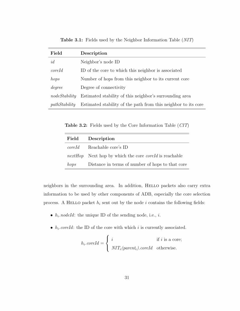
Table 3.1: Fields used by the Neighbor Information Table (NIT)
Field Description
id Neighbor’s node ID
coreId ID of the core to which this neighbor is associated
hops Number of hops from this neighbor to its current core
degree Degree of connectivity
nodeStability Estimated stability of this neighbor’s surrounding area
pathStability Estimated stability of the path from this neighbor to its core
Table 3.2: Fields used by the Core Information Table (CIT)
Field Description
coreId Reachable core’s ID
nextHop Next hop by which the core coreId is reachable
hops Distance in terms of number of hops to that core
neighbors in the surrounding area. In addition, Hello packets also carry extra
information to be used by other components of ADB, especially the core selection
process. A Hello packet hi sent out by the node i contains the following fields:
• hi.nodeId : the unique ID of the sending node, i.e., i.
• hi.coreId : the ID of the core with which i is currently associated.
hi.coreId =
i if i is a core;
NITi(parenti).coreId otherwise.
31
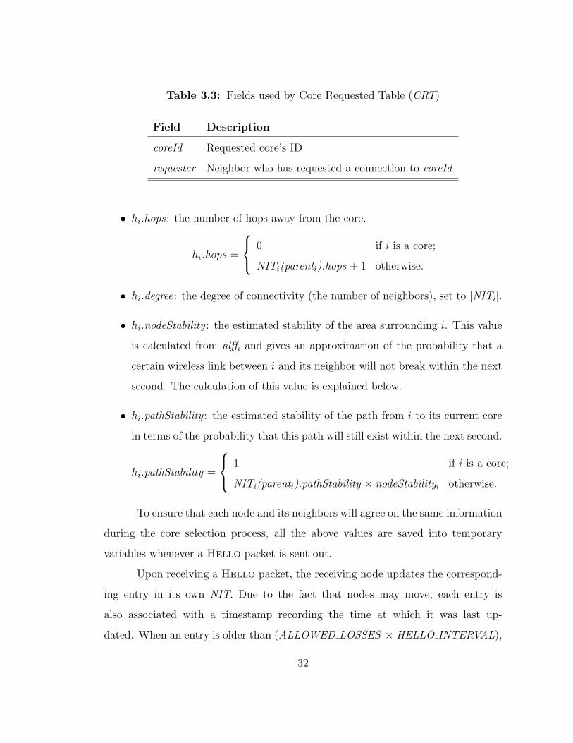
Table 3.3: Fields used by Core Requested Table (CRT)
Field Description
coreId Requested core’s ID
requester Neighbor who has requested a connection to coreId
• hi.hops : the number of hops away from the core.
hi.hops =
0 if i is a core;
NITi(parenti).hops + 1 otherwise.
• hi.degree: the degree of connectivity (the number of neighbors), set to |NITi|.
• hi.nodeStability : the estimated stability of the area surrounding i. This value
is calculated from nlffi and gives an approximation of the probability that a
certain wireless link between i and its neighbor will not break within the next
second. The calculation of this value is explained below.
• hi.pathStability : the estimated stability of the path from i to its current core
in terms of the probability that this path will still exist within the next second.
hi.pathStability =
1 if i is a core;
NITi(parenti).pathStability × nodeStabilityi otherwise.
To ensure that each node and its neighbors will agree on the same information
during the core selection process, all the above values are saved into temporary
variables whenever a Hello packet is sent out.
Upon receiving a Hello packet, the receiving node updates the correspond-
ing entry in its own NIT. Due to the fact that nodes may move, each entry is
also associated with a timestamp recording the time at which it was last up-
dated. When an entry is older than (ALLOWED LOSSES × HELLO INTERVAL),
32
it is removed from the table, which also results in a link failure event. Every
NLFF TIME WINDOW time period, the number of link failures is used to cal-
culate nlff as shown in (3.1) and (3.2) above.
By maintaining nlff, each node i is able to roughly estimate the stability of its
surrounding area by calculating nodeStabilityi which expresses the probability that
a certain wireless link between i and its neighbor will not break within the next
second. Although GPS could be used to obtain more accurate estimation, using
GPS may not be suitable in many situations, especially for smaller devices due to
GPS’ high energy consumption. Without knowing nodes’ geographical locations
(via GPS or any other means) or mobility speeds, nodeStabilityi, which is to be
incorporated into each outgoing Hello packet, is calculated as follows.
For simplicity, we model the time interval node i will wait before detecting
the next link failure by the exponential distribution with the average rate of λi
failures per second. Therefore, the probability that no link failure will be detected
within the next t seconds is e−λit. Since nodeStabilityi gives an approximation of
the probability that a particular link of i will not break within the next second, if i
currently has Ni neighbors, we have
(nodeStabilityi)Ni = e−λi .
Therefore,
nodeStabilityi = e− λi
Ni . (3.3)
Here, λi can be estimated by the actual number of link failures detected per second.
Since Ni is actually |NITi|, it follows from (3.1), (3.2) and (3.3) that
nodeStabilityi = e−nlffi . (3.4)
Notice that the exponential distribution used here to model link failures may
not perfectly predict the actual link failure probability. However, as stated earlier,
33
the desired behavior of ADB is to form smaller clusters in more dynamic areas, and
larger clusters in more static areas. Although there exist more accurate mechanisms
(e.g., [GdWFM02]) to predict link stability, this model serves as an easy-to-calculate
indicator (due to the memoryless property of the exponential distribution) effective
enough2 for ADB to achieve its objective under different mobility conditions. This
has been validated by simulation, as shown in Figure 3.1 for instance.
3.1.3 Core Selection Process
The core selection process at each node begins after the node has started for a
certain waiting period, usually long enough to allow the node to have heard Hello
packets from all of its neighbors. This process decides whether a node should still
be serving as a core, or become a child of an existing core by checking for its own
local optimality. First, each node computes its own height from its current status.
The height metric should be well chosen to suit the application exploiting ADB.
For example, it can be a combination of the remaining energy, the node stability,
and the degree of connectivity. The node ID is always included in the calculation
to break ties. Similar to VDBP, we used (nodeStabilityi, degreei, i) as the height
metric for the node i in ADB. A height will also be calculated by the node i for
each entry in NITi. As mentioned in the previous section, when calculating its
own height, each node acquires its status that was saved in the temporary variables
at the moment the last Hello packet was sent out, rather than using its current
status. Doing so will ensure that all surrounding nodes agree on the same height
information, and avoid potential loop formation when the parent-child relationship
is established among nodes. If a node has the highest height among its neighbors,
2 Our goal is not to have ‘absolute’ accurate prediction which may require morecomplicated computation and additional information to be collected. Instead,we would like to have a simple indicator that can differentiate node and pathstability in a ‘relative’ sense.
34
it is considered a local optimal node and should continue serving as a core. If not,
the node picks the local optimal node as a core and updates its parent variable. All
subsequent Hello packets will be changed accordingly.
While keeping the number of cores as low as possible, the core selection
process has to ensure that the current backbone configuration satisfies two con-
straints: the hop count limit and the path stability. These two constraints are used
to ensure that the hop count and the path stability from every node to its core must
not exceed the parameters HOP THRESHOLD and STABILITY THRESHOLD,
respectively. Therefore, once the local optimality check has been made, each node
must keep listening to the incoming Hello packets. For convenience, we define a
predicate MeetConstraintsi(j) to indicate whether node i would meet the backbone
constraints if it chose node j as its parent. Formally, this predicate is defined as
follows:
MeetConstraintsi(j) ⇐⇒ (i = j) ∨
[NITi(j).hops < HOP THRESHOLD ∧
NITi(j).pathStability > STABILITY THRESHOLD ],
where ∧ and ∨ denote the conventional boolean operations “and” and “or,” respec-
tively. Upon receiving a Hello packet, hj, from node j, node i modifies its local
variables based on the following conditions:
• Condition 1: (j = parenti) ∧ (MeetConstraintsi(j) = FALSE).
This condition implies that the association of node i with its current parent
j has now violated the backbone constraints. Therefore, node i has to find a
new parent k, where k 6= j and MeetConstraintsi(k) is true, with a minimum
number of hops to the core. If no satisfactory parent can be found, node i
becomes a core by setting parenti to i.
35
• Condition 2: (j 6= parenti) ∧ (i 6= parenti) ∧ (hj.hops < NITi(parenti).hops)
∧ (MeetConstraintsi(j) = TRUE).
Here, node i, which is currently not a core, has just heard a Hello packet
from node j who is not its parent but has a shorter distance to the core. Node
i then sets parent i to j.
• Condition 3: (i = parenti)∧(hj.coreId 6= i)∧(MeetConstraintsi(j) = TRUE).
This condition tells that node i, which is currently a core, has heard a Hello
packet from node j that belongs to another core, and node i could associate
itself to j without violating the constraints. If this condition holds, node i will
set parent i to j; otherwise it remains a core.
In the case of mobility, if a node detects that its parent has moved out of
range (from the neighbor discovery process), it will do the same thing as if its parent
violates the constraints (i.e., Condition 1). With different mobility conditions, the
core selection process will result in different numbers of cores and depths of trees
due to the path stability constraint. Figure 3.1(a) depicts a snapshot of the core
selection process on a network of 30 stationary nodes, where there are only two cores
and a larger tree is formed. In contrast, node mobility causes formation of smaller
trees due to the path stability constraint, which results in more cores, as shown in
Figure 3.1(b).
3.1.4 Core Connection Process
Nodes which are selected to become cores by the core selection process cannot
form a connected backbone by themselves, since they may not be reachable by one
another within a single hop. The core connection process is responsible for connect-
ing these cores together by designating some nodes to take the role of intermediate
nodes. Consequently, the cores and intermediate nodes jointly comprise a virtual
36

(a)
(b)
Figure 3.1: Different backbone structures under different mobility speeds (the
larger black nodes represent the cores): (a) mobility speed is 0 m/s,
and (b) mobility speed is 20 m/s.
37

B
C
A
Figure 3.2: Example illustrating the core connection process: Cores A, B, and C
(shown in black) are connected by eight intermediate nodes (shown in
gray) and form a virtual backbone (represented by thick lines). Solid
lines denote parent-child relationship; and dashed circles denote core
coverage boundaries.
backbone, as illustrated in Figure 3.2. To do so, each core relies on nodes that
are located along the border of its coverage, or border nodes, to collect information
about surrounding nearby cores. A node is said to be a border node if and only
if it is able to hear Hello packets from nodes that are associated with different
cores. Each border node then builds a list of cores reachable by itself, including the
next hop and the number of hops to each core, and reports this information to its
own core so that a core connection request can be performed. To reduce overhead,
a border node only needs to collect and report information regarding nearby cores
with IDs lower than that of its own core. Hence, a core connection request between
a pair of cores is always initiated by the core with the higher ID.
In ADB, the core connection process relies on Hello packets to carry two
extra pieces of information: CoreInfo and CoreRequest tables. Algorithm 3.1
38
(presented in pseudo code) illustrates how this information is piggybacked onto out-
going Hello packets, and Algorithm 3.2 describes how this information is processed
at receiving nodes. The following is the detailed explanation. Let coreIdi be
NITi(parenti).coreId if i is not a core, or i otherwise. When node i hears a Hello
packet, hj, from another node j and hj.coreIdj < coreIdi, node i will insert into its
CITi (Core Information Table) an entry 〈hj.coreIdj, j, hj.hops+1〉, which represent
coreId, nextHop, and hops fields, respectively, as described in Table 3.2. This step
corresponds to lines 16–17 of Algorithm 3.1. To propagate this information to the
core, node i piggybacks onto its outgoing Hello packet a CoreInfo table contain-
ing a list of entries 〈coreId,hops〉. Each entry indicates the shortest distance in terms
of the number of hops from node i to each unique core in CITi, as shown in lines
21–24 of Algorithm 3.2. Note that CITi may contain multiple entries for the same
core, but node i will choose only one with the least number of hops to that core.
When any node j hears the Hello packet containing the CoreInfo from node i,
node j looks for entries with lower core IDs than its own and inserts/updates the
corresponding entries in CITj using i as the nextHop field as long as the following
two conditions hold: (1) nodes i and j belong to the same core, and (2) the distance
from node j to the core is less than that of node i. Lines 18–21 of Algorithm 3.1
denotes these steps. Nodes who are not cores and having nonempty CIT tables
must always generate and piggyback CoreInfo tables onto outgoing Hello pack-
ets so that each core can collect all information it needs, and establish connectivity
to nearby cores (again, in lines 21–24 of Algorithm 3.2). Due to the dynamics of
the core selection process and the network topology itself, the CIT table is kept
updated by having each node remove all the entries with nextHop field set to k
when it receives a link failure notification regarding to the node k. In addition, it
also removes all the entries in CIT that match the pattern 〈c, k, ·〉 when it hears a
CoreInfo from k without any entry regarding the core c.
39

Algorithm 3.1 Node i processing Hello packets1: Input:
2: h← incoming Hello
3: src← the sender of h
4: Begin:
5: coreInfo ← CoreInfo piggybacked by h
6: coreReq ← CoreRequest piggybacked by h
7: if parenti = i then /* i is a core */
8: coreIdi ← i
9: hopsi ← 0
10: else /* i is not a core */
11: coreIdi ← NITi(parenti).coreId
12: hopsi ← NITi(parenti).hops + 1
13: end if
14: remove all entries 〈cid, nextHop, hops〉 from CITi where nextHop = src
15: remove all entries 〈cid, requester〉 from CRTi where requester = src
16: if h.coreId < coreIdi then
17: insert 〈h.coreId, src, h.hops+1〉 into CITi
18: else if h.coreId = coreIdi & h.hops > hopsi then
19: for each 〈cid, hops〉 in coreInfo, where cid < coreIdi do
20: insert 〈cid, src, hops+1〉 into CITi
21: end for
22: end if
23: for each 〈cid, nextHop〉 in coreReq where nextHop = i do
24: insert 〈cid, src〉 into CRTi
25: end for
40
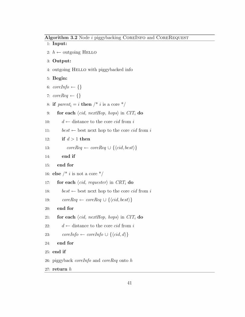
Algorithm 3.2 Node i piggybacking CoreInfo and CoreRequest1: Input:
2: h← outgoing Hello
3: Output:
4: outgoing Hello with piggybacked info
5: Begin:
6: coreInfo ← {}
7: coreReq ← {}
8: if parenti = i then /* i is a core */
9: for each 〈cid, nextHop, hops〉 in CITi do
10: d← distance to the core cid from i
11: best← best next hop to the core cid from i
12: if d > 1 then
13: coreReq ← coreReq ∪ {〈cid, best〉}
14: end if
15: end for
16: else /* i is not a core */
17: for each 〈cid, requester〉 in CRTi do
18: best← best next hop to the core cid from i
19: coreReq ← coreReq ∪ {〈cid, best〉}
20: end for
21: for each 〈cid, nextHop, hops〉 in CITi do
22: d← distance to the core cid from i
23: coreInfo ← coreInfo ∪ {〈cid, d〉}
24: end for
25: end if
26: piggyback coreInfo and coreReq onto h
27: return h
41
Once a core has had information about other surrounding cores stored in its
CIT table, it is able to initiate the connection request to those cores by piggybacking
a CoreRequest table onto each of its outgoing Hello packets. A CoreRequest
table contains a list of entries 〈coreId,nextHop〉, each of which indicates which node
is being requested to connect to each unique core from the CIT table, as shown
in lines 8–15 of Algorithm 3.2. Similar to the construction of a CoreInfo table,
only one next hop with the shortest distance in terms of the number of hops is
chosen for each core. Entries from CIT with one hop count are excluded from the
CoreRequest table since they represent other cores with direct contact, which
do not require any intermediate nodes to establish connectivity with. When node
i receives a Hello packet containing a CoreRequest table from node j, node i
checks for entries where its ID appears on the nextHop field. For each entry 〈c, i〉
found in the CoreRequest, node i inserts into CRTi (Core Request Table) an entry
with coreId and requester set to c and j, respectively (Algorithm 3.1, lines 23–25).
Each node i who is not a core and has at least one entry in its CRTi is required
to construct a CoreRequest table with entries corresponding to all the cores in
CRTi (Algorithm 3.2, lines 17–20). For each entry 〈c, nc〉 in the CoreRequest
table that node i is to generate, if node c is the current core of node i, node i will
use parenti as the value of nc; otherwise node i will consult its CITi for the best
next hop to node c.
Similar to the maintenance of CIT, when node i detects that the link to node
k has failed, node i removes from CRTi all the entries whose requester fields are
equal to k. If CRTi contains an entry 〈c, k〉 but node i hears a CoreRequest
table from node k without an entry 〈c, i〉, the entry 〈c, k〉 is removed from CRTi.
Node i determines if it is currently on the backbone by checking if it is either
a core (parenti = i) or an intermediate node (|CRTi| > 0). These nodes on the
backbone play an important role for facilitating multicast operations, which will be
42
Table 3.4: Fields used by the Join Table (JT)
Field Description
groupId Multicast group ID
requester Node who has requested to join this group
described in the next section.
3.2 ADBM – Multicast Routing over ADB
This section describes how the proposed multicast protocol, called ADBM
(ADB-based Multicast), can exploit the backbone infrastructure provided by ADB
to achieve mobility-adaptive multicast routing for ad hoc networks. As resulted from
ADB, each node is either a core or has an association to a core which is reachable
via its parent node. In addition, cores are already connected via intermediate nodes
by the core connection process. Given this backbone infrastructure, a node willing
to join a multicast group sends a request toward its core via its parent to ask
the intermediate nodes between itself and the core to become forwarding nodes for
the multicast group. Group members are therefore connected via the backbone.
The following subsections explain the group joining and data packet forwarding
mechanisms in turn.
3.2.1 Group Joining
In addition to the data structures for ADB described in Section 3.1.1, each
node maintains a join table which has the same structure as a core request table
(Table 3.3) with a group ID field instead of a core ID, as shown in Table 3.4. For
node i, its join table is denoted by JTi. The group joining mechanism is based on the
concept of rendezvous points, where control messages are directed toward the core of
the group instead of being broadcast to other irrelevant nodes or the entire network.
43

Backbone
normal non−core node
multicast group member
core
multicast group forwarder
join branch
������������
������������������������ ���
���������
Figure 3.3: An example showing nodes forming of multicast trees, which are con-
nected by the backbone, during group joining process
Here, the rendezvous point for each node is its current core. Node i who is willing to
join a multicast group informs its parent by piggybacking a JoinRequest, along
with its parent ID, parenti, onto its outgoing Hello packets. The JoinRequest
contains a list of all multicast group IDs that node i has joined and is willing to
join. The JoinRequest also includes group IDs of which i is currently a forwarding
node. When a node j receives a Hello with a JoinRequest, it checks if its ID
is specified as the intended receiver of the JoinRequest. If so, node j updates its
JTj with all the entries found in the JoinRequest received from node i, using i as
the requester field. It is required that nodes who are members of some groups, and
any nodes whose join tables are not empty, with the exception for cores, periodically
broadcast JoinRequest with their Hello messages. A node who has an entry for
the group ID g in its join table then marks itself as a forwarding node for group
g, and nodes on the backbone are considered forwarding nodes for any group. As
a result, these forwarding nodes form a multicast tree within each core’s coverage,
where multiple trees are connected by the backbone, hence establishing connectivity
among the group members, as illustrated in Figure 3.3.
To deal with network dynamics, the join table is maintained in the same
way as ADB does to CIT and CRT in that entries whose requester fields are i are
44

removed from the table whenever a link to node i has broken. The entry with groupId
and requester set to g and i, respectively, is also removed when a JoinRequest
received from node i contains no entry for the group g.
3.2.2 Multicast Packet Forwarding
Although multicast connectivity establishment within a core’s coverage re-
sembles a tree formation, ADBM protocol allows forwarding nodes and members
to accept data packets that arrive from any node. (Hence it is considered a mesh-
based protocol.) Since there can exist more than one path between a sender and a
receiver, each data packet is assigned a unique sequence number when it is leaving
its source. The sequence numbers are checked by each forwarding node and member
node to ensure that no duplicate data packets are rebroadcast or delivered to the
application. When a node i receives a non-duplicate data packet for the group g, it
checks whether it is currently a forwarding node of the group, i.e., whether one or
more of the following conditions hold:
• node i is a core, i.e., parenti = i.
• node i is an intermediate node on the backbone, i.e., |CRTi| > 0.
• node i has an entry for g in its join table.
If so, node i rebroadcasts the packet. Otherwise, the packet is silently dis-
carded. If node i is a member of the group g and none of the above conditions hold,
node i will deliver the packet to the application without rebroadcasting.
3.3 Performance Evaluation
We have conducted simulation experiments using the QualNet simulator [Sca]
to study the performance of ADBM with different environment and application
settings.
45
3.3.1 Simulation Model
We evaluated performance of ADBM over 20 randomly generated networks,
each of which consisted of 50 nodes uniformly distributed over a terrain of size
1000×1000 m2. Each node was equipped with a radio transceiver which was capa-
ble of transmitting up to approximately 250 meters over a 2 Mbps wireless channel,
assuming two-ray path loss model without fading. We used IEEE 802.11DCF as the
MAC layer protocol, and IP as the network layer which supported only fragmenta-
tion and communication with immediate neighbors. Since ADBM protocol does not
rely on any unicast protocol, no other routing protocol was provided. There was
only one multicast session running with different numbers of group members. Mem-
bers were randomly selected from the 50 nodes and joined the group all at the same
time after the simulation had started for 5 seconds until the end. In all experiments
except the one that studies the effect of number of senders, three group members
were chosen as multicast senders, each of which was configured to start generating
a constant bit rate (CBR) traffic of 5 packets/sec (unless stated otherwise) after
the simulation started for 10 seconds. The size of data payload was 512 bytes and
each multicast session would last for 200 seconds. In each experiment with mobility,
all nodes were moving continuously at a specific speed. Table 3.5 shows the fixed
protocol parameters used in all but the first two experiments where the effects of
HOP THRESHOLD and STABILITY THRESHOLD parameters are studied.
The following statistics were collected to study ADBM performance, where
each measurement is shown with a 95% confidence interval:
• Packet delivery ratio: The ratio of the number of non-duplicate data pack-
ets successfully delivered to the receivers versus the number of packets sup-
posed to be received. This metric reflects the effectiveness of a protocol.
• Number of total packets transmitted per data packet received: The
ratio of the number of data and control packets transmitted versus the number
46

Table 3.5: Fixed parameter values for ADBM
HELLO INTERVAL 1 sec
ALLOWED LOSSES 1
NLFF TIME WINDOW 2 secs
α 0.6
HOP THRESHOLD 2
STABILITY THRESHOLD 0.98
of data packets successfully delivered to the application. Hello packets are
also considered as packets transmitted. This measure shows efficiency of a
protocol in terms of channel access. The lower the number, the more efficient
the protocol.
• Number of total bytes transmitted per data byte received: This metric
is similar to the second metric except that the number of bytes is considered
instead. Here, bytes transmitted include everything that is sent to the MAC
layer (i.e., IP and UDP headers, as well as Hello packets), where data bytes
received involve only the data payloads. This metric presents efficiency of a
protocol in terms of bandwidth utilization. Similar to the second metric, the
lower the number, the more efficient the protocol.
For the comparison purpose, we have also performed experiments on an ex-
isting multicast protocol, ODMRP (On-Demand Multicast Routing Protocol). As
mentioned in Chapter 2, ODMRP is an on-demand, mesh-based multicast protocol
that extracts a subset of nodes, called a forwarding group, only when a source of
the group has data to send. The nodes in the forwarding group form a mesh that
connects the group members together. When a multicast source has data to send for
47
the first time, it broadcasts to its neighbors a Join Query packet, which is a data
packet with the query flag set. Upon receiving a non-duplicate Join Query, each
node stores the upstream node ID in its routing table and rebroadcasts the packet.
When a member of the multicast group receives a Join Query, it constructs and
broadcasts a Join Reply packet containing the source ID and the upstream node
ID to all of its neighbors. Upon receiving a Join Reply, a node whose ID matches
the upstream ID in the packet realizes that it is on the path between the source and
a member, so it becomes a forwarding node for the group by setting its FG FLAG
(Forwarding Group Flag). It then constructs and broadcasts its own Join Reply
using its corresponding upstream node ID. The broadcasting of Join Reply pack-
ets therefore propagates the information from all the members back to the source
on the reverse paths. Once the source has sent out a Join Query, it sends all
subsequent data packets normally with no query flag set. This will allow only nodes
that are currently in the forwarding group to rebroadcast these data packets, thus
reducing data forwarding overhead. To deal with dynamics of the network topology
and group membership, each source floods the network with Join Querys every
REFRESH INTERVAL as long as it still has data to be sent to the group. The
FG FLAG on each node will be reset if it has not been refreshed by Join Reply
for some period of time, which implies that the source has no data to send, or the
node itself is no longer needed as a forwarding node. If nodes are equipped with
GPS, a mobility prediction method can also be used to adaptively adjust the value
of REFRESH INTERVAL to suit the current mobility condition.
In this comparison, we used QualNet’s implementation of ODMRP, which
followed the specification in the Internet Draft draft-ietf-manet-odmrp-02.txt
[LSG00] but without mobility prediction which requires GPS. The value of RE-
FRESH INTERVAL was fixed at 3 seconds.
48
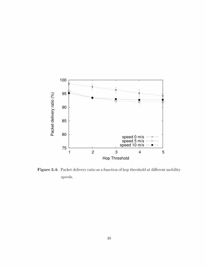
75
80
85
90
95
100
1 2 3 4 5
Pac
ket d
eliv
ery
ratio
(%)
Hop Threshold
speed 0 m/sspeed 5 m/s
speed 10 m/s
Figure 3.4: Packet delivery ratio as a function of hop threshold at different mobility
speeds.
49

0
0.2
0.4
0.6
0.8
1
1.2
1.4
1.6
1.8
2
1 2 3 4 5Tota
l pkt
s tra
nsm
itted
per
dat
a pk
t rec
eive
d
Hop Threshold
speed 0 m/sspeed 5 m/s
speed 10 m/s
Figure 3.5: Number of total packets transmitted per data packet delivered as a
function of hop threshold at different mobility speeds.
50
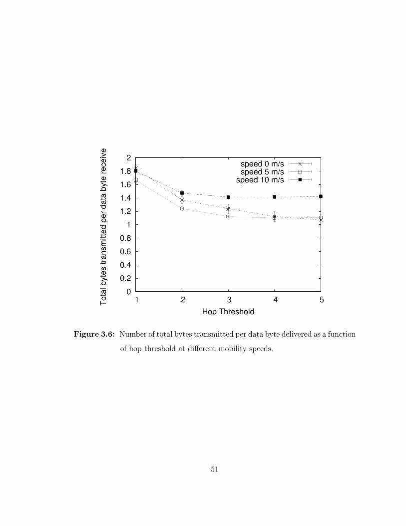
0
0.2
0.4
0.6
0.8
1
1.2
1.4
1.6
1.8
2
1 2 3 4 5Tota
l byt
es tr
ansm
itted
per
dat
a by
te re
ceiv
ed
Hop Threshold
speed 0 m/sspeed 5 m/s
speed 10 m/s
Figure 3.6: Number of total bytes transmitted per data byte delivered as a function
of hop threshold at different mobility speeds.
51
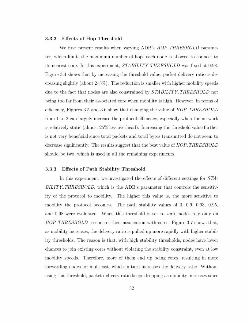
3.3.2 Effects of Hop Threshold
We first present results when varying ADB’s HOP THRESHOLD parame-
ter, which limits the maximum number of hops each node is allowed to connect to
its nearest core. In this experiment, STABILITY THRESHOLD was fixed at 0.98.
Figure 3.4 shows that by increasing the threshold value, packet delivery ratio is de-
creasing slightly (about 2–3%). The reduction is smaller with higher mobility speeds
due to the fact that nodes are also constrained by STABILITY THRESHOLD not
being too far from their associated core when mobility is high. However, in terms of
efficiency, Figures 3.5 and 3.6 show that changing the value of HOP THRESHOLD
from 1 to 2 can largely increase the protocol efficiency, especially when the network
is relatively static (almost 25% less overhead). Increasing the threshold value further
is not very beneficial since total packets and total bytes transmitted do not seem to
decrease significantly. The results suggest that the best value of HOP THRESHOLD
should be two, which is used in all the remaining experiments.
3.3.3 Effects of Path Stability Threshold
In this experiment, we investigated the effects of different settings for STA-
BILITY THRESHOLD, which is the ADB’s parameter that controls the sensitiv-
ity of the protocol to mobility. The higher this value is, the more sensitive to
mobility the protocol becomes. The path stability values of 0, 0.9, 0.93, 0.95,
and 0.98 were evaluated. When this threshold is set to zero, nodes rely only on
HOP THRESHOLD to control their association with cores. Figure 3.7 shows that,
as mobility increases, the delivery ratio is pulled up more rapidly with higher stabil-
ity thresholds. The reason is that, with high stability thresholds, nodes have lower
chances to join existing cores without violating the stability constraint, even at low
mobility speeds. Therefore, more of them end up being cores, resulting in more
forwarding nodes for multicast, which in turn increases the delivery ratio. Without
using this threshold, packet delivery ratio keeps dropping as mobility increases since
52
50
55
60
65
70
75
80
85
90
95
100
0 10 20 30 40 50
Pac
ket d
eliv
ery
ratio
(%)
Mobility Speed (m/s)
threshold=0.0threshold=0.90threshold=0.93threshold=0.95threshold=0.98
Figure 3.7: Packet delivery ratio as a function of mobility at different path stability
thresholds.
53
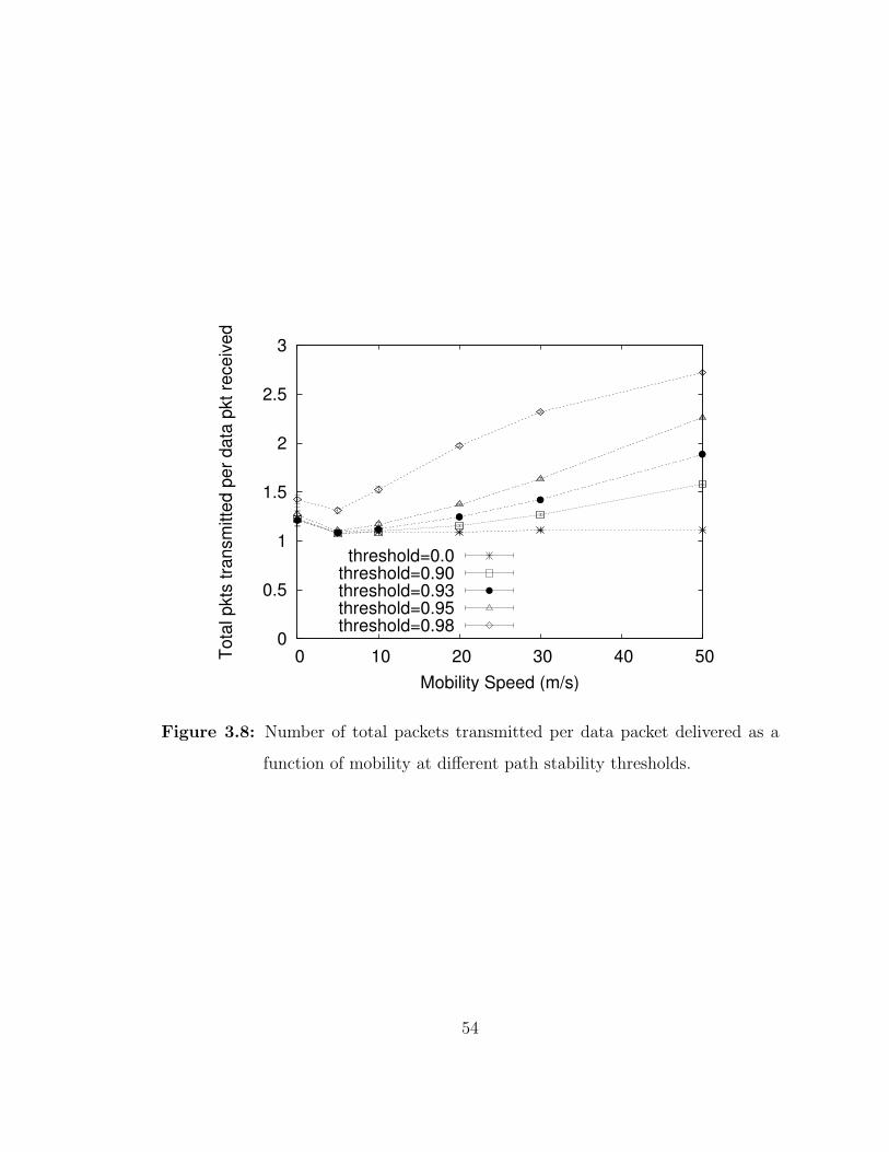
0
0.5
1
1.5
2
2.5
3
0 10 20 30 40 50Tota
l pkt
s tra
nsm
itted
per
dat
a pk
t rec
eive
d
Mobility Speed (m/s)
threshold=0.0threshold=0.90threshold=0.93threshold=0.95threshold=0.98
Figure 3.8: Number of total packets transmitted per data packet delivered as a
function of mobility at different path stability thresholds.
54

0
0.5
1
1.5
2
2.5
3
0 10 20 30 40 50Tota
l byt
es tr
ansm
itted
per
dat
a by
te re
ceiv
ed
Mobility Speed (m/s)
threshold=0.0threshold=0.90threshold=0.93threshold=0.95threshold=0.98
Figure 3.9: Number of total bytes transmitted per data byte delivered as a function
of mobility at different path stability thresholds.
55
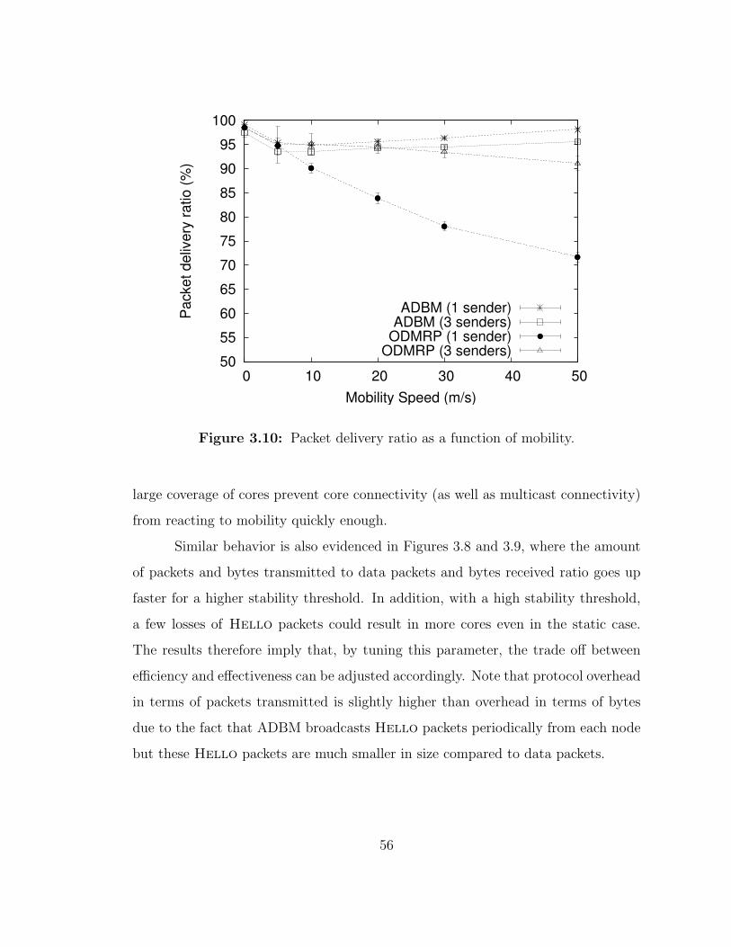
50
55
60
65
70
75
80
85
90
95
100
0 10 20 30 40 50
Pac
ket d
eliv
ery
ratio
(%)
Mobility Speed (m/s)
ADBM (1 sender)ADBM (3 senders)
ODMRP (1 sender)ODMRP (3 senders)
Figure 3.10: Packet delivery ratio as a function of mobility.
large coverage of cores prevent core connectivity (as well as multicast connectivity)
from reacting to mobility quickly enough.
Similar behavior is also evidenced in Figures 3.8 and 3.9, where the amount
of packets and bytes transmitted to data packets and bytes received ratio goes up
faster for a higher stability threshold. In addition, with a high stability threshold,
a few losses of Hello packets could result in more cores even in the static case.
The results therefore imply that, by tuning this parameter, the trade off between
efficiency and effectiveness can be adjusted accordingly. Note that protocol overhead
in terms of packets transmitted is slightly higher than overhead in terms of bytes
due to the fact that ADBM broadcasts Hello packets periodically from each node
but these Hello packets are much smaller in size compared to data packets.
56
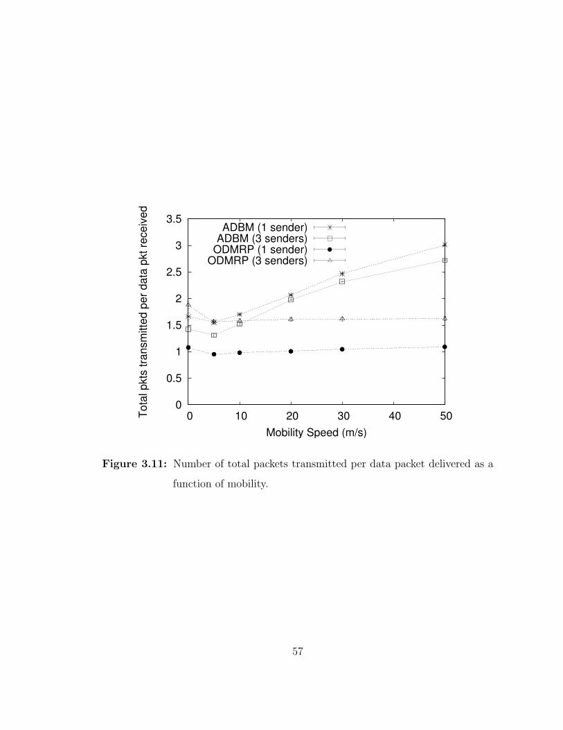
0
0.5
1
1.5
2
2.5
3
3.5
0 10 20 30 40 50Tota
l pkt
s tra
nsm
itted
per
dat
a pk
t rec
eive
d
Mobility Speed (m/s)
ADBM (1 sender)ADBM (3 senders)
ODMRP (1 sender)ODMRP (3 senders)
Figure 3.11: Number of total packets transmitted per data packet delivered as a
function of mobility.
57

0
0.5
1
1.5
2
2.5
3
0 10 20 30 40 50Tota
l byt
es tr
ansm
itted
per
dat
a by
te re
ceiv
ed
Mobility Speed (m/s)
ADBM (1 sender)ADBM (3 senders)
ODMRP (1 sender)ODMRP (3 senders)
Figure 3.12: Number of total bytes transmitted per data byte delivered as a func-
tion of mobility.
58

3.3.4 Effect of Mobility
While the previous experiments are used to study how different values of
ADBM’s parameters impact its behavior, this and the following experiments are
intended to investigate the protocol’s performance under different network and ap-
plication settings. Figure 3.10 shows the packet delivery ratio of both ADBM and
ODMRP with one and three senders under different mobility speeds, varying from 0
to 50 m/s. When the network is static, the protocol can successfully delivery more
than 99% of data packets with one sender, which is reasonable for low traffic. As
mobility increases, the delivery ratio drops by a small amount. However, when the
nodes move faster (around 20 m/s), the delivery ratio goes up again. This is due
to the fact that backbone formation is controlled by the stability threshold. When
stability of the nodes is reduced due to mobility, the coverage of cores gets smaller
accordingly. With more cores in the network, there are more redundant routes from
the sender to the receivers, hence increasing the chance of successful deliveries. The
protocol still performs quite effectively even under extremely high mobility (at 50
m/s). ODMRP, in contrast, yields high packet delivery ratio with one sender in
static networks but loses more packets as mobility increases. An explanation to this
is that in ODMRP the number of nodes that form a multicast mesh depends on the
number of senders in the group. With one sender, meshes are not robust enough to
cope with network dynamics. When there are more senders, ODMRP can handle
mobility better.
Figures 3.11 and 3.12 compare efficiency of ADBM and ODMRP at different
mobility speeds. The results also give an implication on how many forwarding nodes
there are in the network on average. We can see that ADBM performs efficiently
at low speeds, where a low number of data packets are rebroadcast by forwarding
nodes. At higher speeds, more nodes become forwarding nodes due to presence
of more cores, so more data packets are rebroadcast to maintain effectiveness of
59
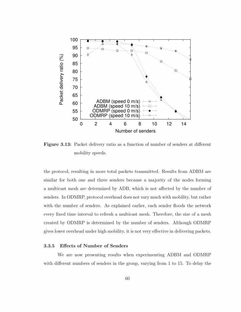
50
55
60
65
70
75
80
85
90
95
100
0 2 4 6 8 10 12 14
Pac
ket d
eliv
ery
ratio
(%)
Number of senders
ADBM (speed 0 m/s)ADBM (speed 10 m/s)ODMRP (speed 0 m/s)
ODMRP (speed 10 m/s)
Figure 3.13: Packet delivery ratio as a function of number of senders at different
mobility speeds.
the protocol, resulting in more total packets transmitted. Results from ADBM are
similar for both one and three senders because a majority of the nodes forming
a multicast mesh are determined by ADB, which is not affected by the number of
senders. In ODMRP, protocol overhead does not vary much with mobility, but rather
with the number of senders. As explained earlier, each sender floods the network
every fixed time interval to refresh a multicast mesh. Therefore, the size of a mesh
created by ODMRP is determined by the number of senders. Although ODMRP
gives lower overhead under high mobility, it is not very effective in delivering packets.
3.3.5 Effects of Number of Senders
We are now presenting results when experimenting ADBM and ODMRP
with different numbers of senders in the group, varying from 1 to 15. To delay the
60
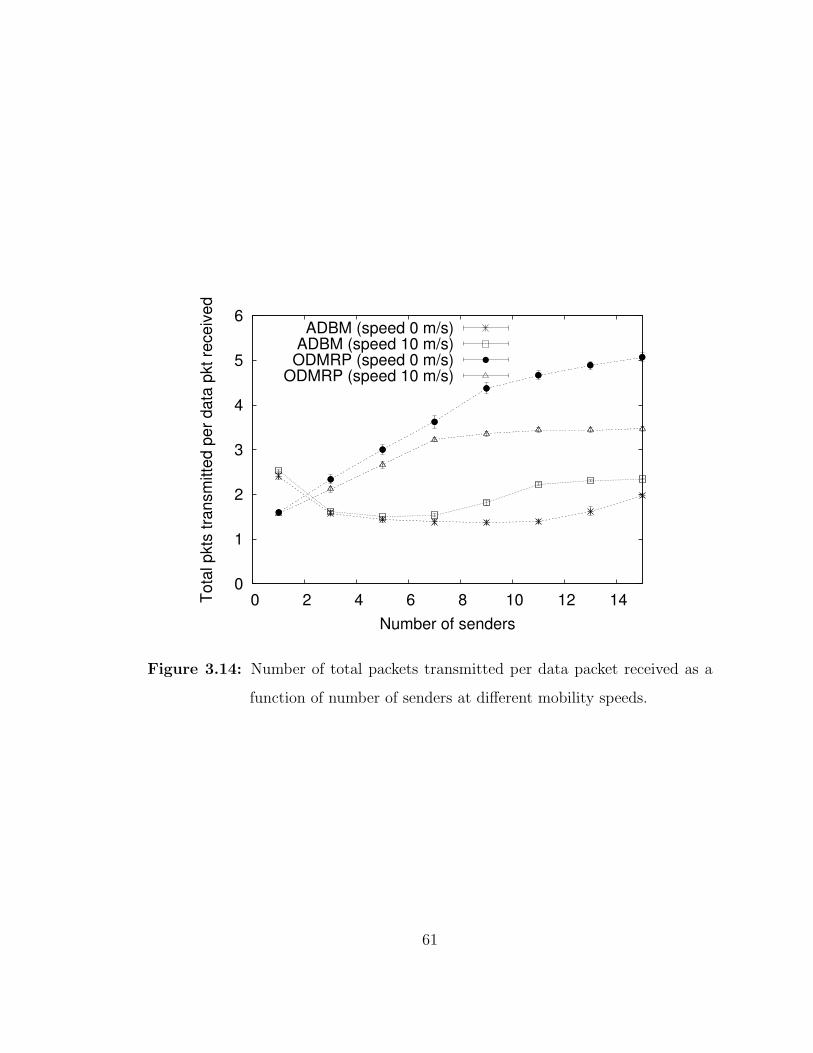
0
1
2
3
4
5
6
0 2 4 6 8 10 12 14Tota
l pkt
s tra
nsm
itted
per
dat
a pk
t rec
eive
d
Number of senders
ADBM (speed 0 m/s)ADBM (speed 10 m/s)ODMRP (speed 0 m/s)
ODMRP (speed 10 m/s)
Figure 3.14: Number of total packets transmitted per data packet received as a
function of number of senders at different mobility speeds.
61

0
1
2
3
4
5
6
0 2 4 6 8 10 12 14Tota
l byt
es tr
ansm
itted
per
dat
a by
te re
ceiv
ed
Number of senders
ADBM (speed 0 m/s)ADBM (speed 10 m/s)ODMRP (speed 0 m/s)
ODMRP (speed 10 m/s)
Figure 3.15: Number of total bytes transmitted per data byte received as a func-
tion of number of senders at different mobility speeds.
62
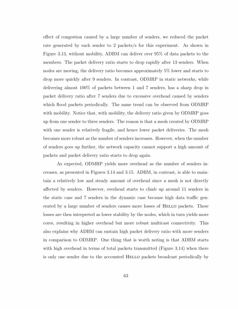
effect of congestion caused by a large number of senders, we reduced the packet
rate generated by each sender to 2 packets/s for this experiment. As shown in
Figure 3.13, without mobility, ADBM can deliver over 95% of data packets to the
members. The packet delivery ratio starts to drop rapidly after 13 senders. When
nodes are moving, the delivery ratio becomes approximately 5% lower and starts to
drop more quickly after 9 senders. In contrast, ODMRP in static networks, while
delivering almost 100% of packets between 1 and 7 senders, has a sharp drop in
packet delivery ratio after 7 senders due to excessive overhead caused by senders
which flood packets periodically. The same trend can be observed from ODMRP
with mobility. Notice that, with mobility, the delivery ratio given by ODMRP goes
up from one sender to three senders. The reason is that a mesh created by ODMRP
with one sender is relatively fragile, and hence lower packet deliveries. The mesh
becomes more robust as the number of senders increases. However, when the number
of senders goes up further, the network capacity cannot support a high amount of
packets and packet delivery ratio starts to drop again.
As expected, ODMRP yields more overhead as the number of senders in-
creases, as presented in Figures 3.14 and 3.15. ADBM, in contrast, is able to main-
tain a relatively low and steady amount of overhead since a mesh is not directly
affected by senders. However, overhead starts to climb up around 11 senders in
the static case and 7 senders in the dynamic case because high data traffic gen-
erated by a large number of senders causes more losses of Hello packets. These
losses are then interpreted as lower stability by the nodes, which in turn yields more
cores, resulting in higher overhead but more robust multicast connectivity. This
also explains why ADBM can sustain high packet delivery ratio with more senders
in comparison to ODMRP. One thing that is worth noting is that ADBM starts
with high overhead in terms of total packets transmitted (Figure 3.14) when there
is only one sender due to the accounted Hello packets broadcast periodically by
63
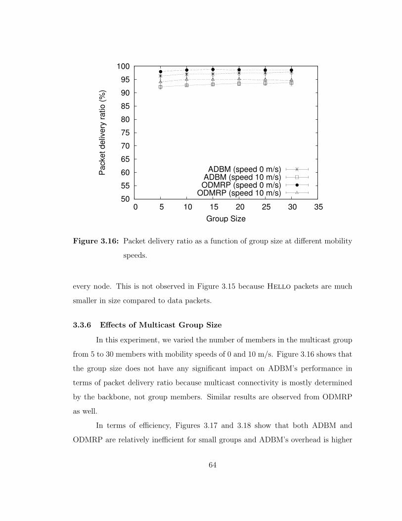
50
55
60
65
70
75
80
85
90
95
100
0 5 10 15 20 25 30 35
Pac
ket d
eliv
ery
ratio
(%)
Group Size
ADBM (speed 0 m/s)ADBM (speed 10 m/s)ODMRP (speed 0 m/s)
ODMRP (speed 10 m/s)
Figure 3.16: Packet delivery ratio as a function of group size at different mobility
speeds.
every node. This is not observed in Figure 3.15 because Hello packets are much
smaller in size compared to data packets.
3.3.6 Effects of Multicast Group Size
In this experiment, we varied the number of members in the multicast group
from 5 to 30 members with mobility speeds of 0 and 10 m/s. Figure 3.16 shows that
the group size does not have any significant impact on ADBM’s performance in
terms of packet delivery ratio because multicast connectivity is mostly determined
by the backbone, not group members. Similar results are observed from ODMRP
as well.
In terms of efficiency, Figures 3.17 and 3.18 show that both ADBM and
ODMRP are relatively inefficient for small groups and ADBM’s overhead is higher
64

0
1
2
3
4
5
6
7
0 5 10 15 20 25 30 35Tota
l pkt
s tra
nsm
itted
per
dat
a pk
t rec
eive
d
Group Size
ADBM (speed 0 m/s)ADBM (speed 10 m/s)ODMRP (speed 0 m/s)
ODMRP (speed 10 m/s)
Figure 3.17: Number of total packets transmitted per data packet received as a
function of group size at different mobility speeds.
65
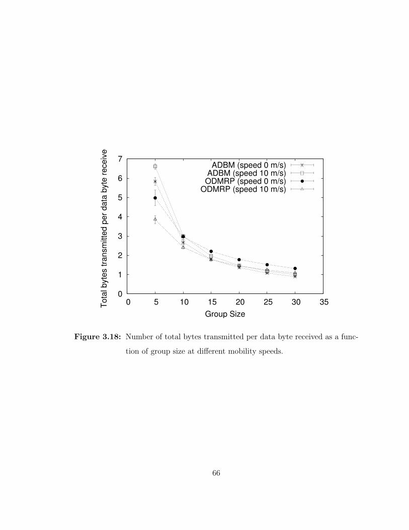
0
1
2
3
4
5
6
7
0 5 10 15 20 25 30 35Tota
l byt
es tr
ansm
itted
per
dat
a by
te re
ceiv
ed
Group Size
ADBM (speed 0 m/s)ADBM (speed 10 m/s)ODMRP (speed 0 m/s)
ODMRP (speed 10 m/s)
Figure 3.18: Number of total bytes transmitted per data byte received as a func-
tion of group size at different mobility speeds.
66

50
55
60
65
70
75
80
85
90
95
100
0 5 10 15 20
Pac
ket d
eliv
ery
ratio
(%)
Traffic Load (pkts/s/sender)
ADBM (speed 0 m/s)ADBM (speed 10 m/s)ODMRP (speed 0 m/s)
ODMRP (speed 10 m/s)
Figure 3.19: Packet delivery ratio as a function of traffic load at different mobility
speeds.
than ODMRP’s. This can be explained by the fact that a backbone is independently
formed by ADB, regardless of the group members. Therefore, there are always
a fixed number of forwarding nodes (i.e., nodes on the backbone) to start with
regardless of the number of members. When the group size grows larger than 10
members, ODMRP’s overhead surpasses that of ADBM since it tends to create
larger meshes as more members join the group.
3.3.7 Effects of Traffic Load
Our last experiment examines performance of ADBM and ODMRP under
different traffic loads, which were between 1 and 20 packets/second/sender. Under
low traffic (less than 7 packets/s), both ADBM and ODMRP give equally high packet
delivery ratio when there is no mobility, as presented in Figure 3.19. At higher loads,
67
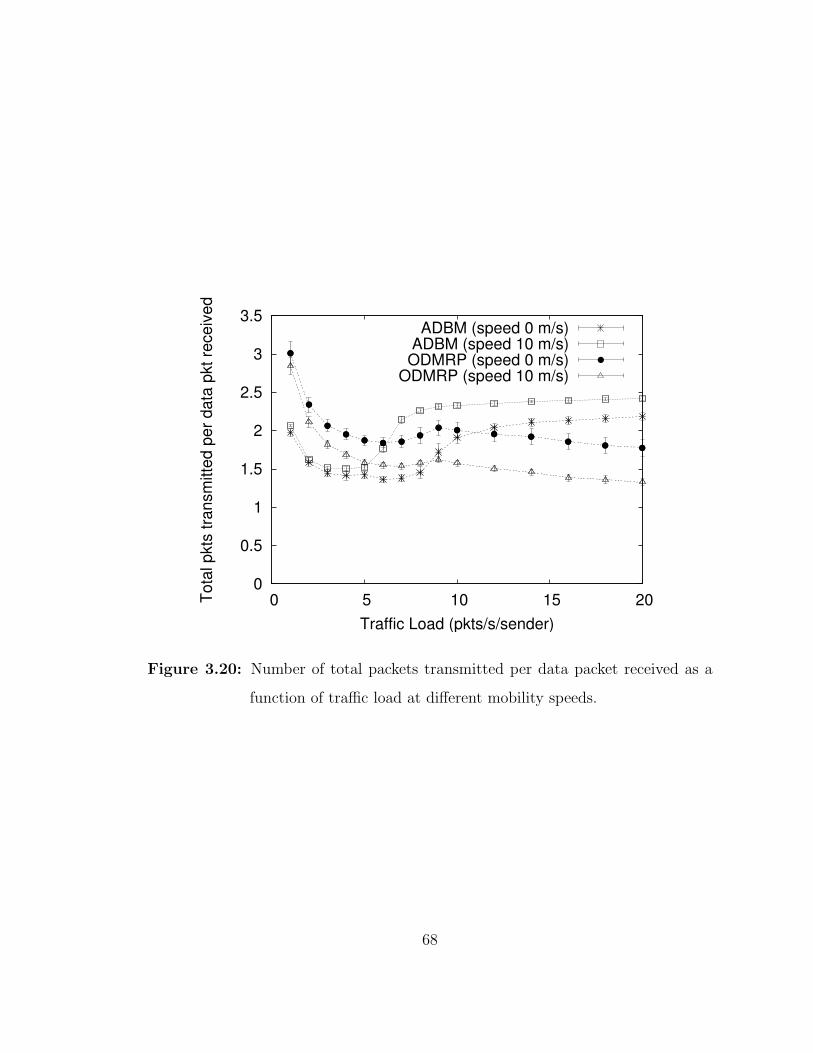
0
0.5
1
1.5
2
2.5
3
3.5
0 5 10 15 20Tota
l pkt
s tra
nsm
itted
per
dat
a pk
t rec
eive
d
Traffic Load (pkts/s/sender)
ADBM (speed 0 m/s)ADBM (speed 10 m/s)ODMRP (speed 0 m/s)
ODMRP (speed 10 m/s)
Figure 3.20: Number of total packets transmitted per data packet received as a
function of traffic load at different mobility speeds.
68

0
0.5
1
1.5
2
2.5
3
3.5
0 5 10 15 20Tota
l byt
es tr
ansm
itted
per
dat
a by
te re
ceiv
ed
Traffic Load (pkts/s/sender)
ADBM (speed 0 m/s)ADBM (speed 10 m/s)ODMRP (speed 0 m/s)
ODMRP (speed 10 m/s)
Figure 3.21: Number of total bytes transmitted per data byte received as a func-
tion of traffic load at different mobility speeds.
69
packet delivery ratio from both protocols drops rapidly, while ODMRP has a sharper
drop than ADBM. This can be explained by Figures 3.20 and 3.21 which show that
ADBM starts transmitting more packets when the data rate is above 8 packets/s,
which implies that more nodes become forwarding nodes. As a result, multicast
connectivity provided by ADBM is more robust than that of ODMRP under high
loads. With mobility, we can observe similar results from both protocols in terms
of their reactions to increasing traffic loads. However, ADBM has about 2-5% lower
packet delivery ratio than ODMRP in almost every traffic setting.
3.4 Summary
We have introduced a novel mobility-adaptive multicast protocol for mobile
ad hoc networks. The protocol, based on a two-tier architecture, uses the proposed
adaptive dynamic backbone algorithm (ADB) to construct a virtual backbone in-
frastructure to facilitate multicast operations. ADB extracts a subset of nodes,
called backbone nodes or cores, out of the network. These cores then establish con-
nectivity among one another to form a virtual infrastructure. Each core is allowed
to have larger coverage in relatively static areas, while the coverage is reduced in
more dynamic areas so that connectivity among cores can be efficiently established
and quickly reestablished under high mobility. The multicast protocol, ADBM, em-
ploys the provided backbone infrastructure to achieve adaptive multicast routing
which integrates a tree-based scheme and a flooding scheme together to provide
both efficiency in static areas and robustness in dynamic areas, even within the
same network. Since every node is either a core or has an association to a core
via its parent node, cores are also used to avoid global flooding of control messages
triggered by a node’s joining a group or maintaining group membership, as found in
other on-demand multicast protocols. It has been shown via simulation that ADBM
performs efficiently under low mobility and still effectively under extremely high mo-
bility with various network and application settings. In comparison to ODMRP—an
70

existing ad hoc multicast protocol, ADBM reacts to mobility more effectively and
has better performance in terms of both effectiveness and efficiency with a large
number of senders.
71
Chapter 4
MULTICAST WITH SWARM INTELLIGENCE
In mobile wireless ad hoc networks, where resources such as energy and band-
width are scarce, it is preferred that networking protocols are resource aware. From
the aspect of multicast routing, multicast protocols should be able to establish effi-
cient connectivity among group members with an acceptable level of overhead. One
way to achieve this is to find a subset of nodes that can be used to connect all the
group members together while yielding the minimum total “cost.” However, finding
such a minimum-cost subset is similar to the Steiner tree problem [BKJ83, LcK00],
which is known to be NP-hard. Although several heuristics have been proposed,
they often rely on global knowledge of network topology to perform the calculation.
In this chapter, we describe a novel multicast routing protocol for mobile ad
hoc networks that adopts swarm intelligence to reduce the number of nodes used to
establish multicast connectivity. We name the protocol Multicast for Ad hoc Net-
works with Swarm Intelligence or MANSI for short. As mentioned in Section 2.2,
swarm intelligence refers to complex behaviors that arise from simple interactions
among individuals, such as ants, but often achieves global optimization objectives.
Similarly, MANSI utilizes small control packets equivalent to ants in the physical
world. These packets, traveling like biological ants, deposit control information at
nodes they visit, similar to the way ants laying pheromone trails. This informa-
tion, in turn, affects the behavior of other ant packets. With this form of indirect
communication (known as stigmergy), the deployment of ant-like packets resembles
72
an adaptive distributed control system that evolves itself to a more efficient state,
accommodating the current condition of the environment.
For each multicast group, MANSI determines a set of intermediate nodes,
forming a forwarding set, that connect group members together and are shared
among group senders. By adopting a core-based approach, the forwarding set is
initially formed by nodes that are on the shortest paths between the core and the
other group members, where the core may be one of the group members or senders.
In addition, during the lifetime of the multicast session (i.e., when there is at least
one active sender), the forwarding set will evolve, by means of swarm intelligence,
over time into states that yield lower cost, which is expressed in terms of total
cost of all the nodes in the forwarding set. This evolving, including exploring and
learning, mechanism differentiates MANSI from other existing ad hoc multicast
routing protocols. Since a node’s cost is abstract and may be defined to represent
different metrics, MANSI can be applied to many variations of multicast routing
problems for ad hoc networks such as load balancing, secure routing, and energy
conservation.
The next section describes the motivation and overview of the MANSI pro-
tocol.
4.1 Overview of MANSI
MANSI is an on-demand multicast routing protocol that creates a multicast
connection among group members by determining a set of intermediate nodes that
serve as forwarding nodes. This set, called a forwarding set, is shared among all
the senders of the group. The protocol exploits a core-based technique where each
member joins the group via the core node to establish a connection with the other
group members. Unlike the core-based tree (CBT) protocol [BFC93], however, the
core of each group is not statically assigned to a particular node in the network
73
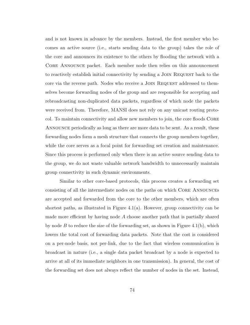
and is not known in advance by the members. Instead, the first member who be-
comes an active source (i.e., starts sending data to the group) takes the role of
the core and announces its existence to the others by flooding the network with a
Core Announce packet. Each member node then relies on this announcement
to reactively establish initial connectivity by sending a Join Request back to the
core via the reverse path. Nodes who receive a Join Request addressed to them-
selves become forwarding nodes of the group and are responsible for accepting and
rebroadcasting non-duplicated data packets, regardless of which node the packets
were received from. Therefore, MANSI does not rely on any unicast routing proto-
col. To maintain connectivity and allow new members to join, the core floods Core
Announce periodically as long as there are more data to be sent. As a result, these
forwarding nodes form a mesh structure that connects the group members together,
while the core serves as a focal point for forwarding set creation and maintenance.
Since this process is performed only when there is an active source sending data to
the group, we do not waste valuable network bandwidth to unnecessarily maintain
group connectivity in such dynamic environments.
Similar to other core-based protocols, this process creates a forwarding set
consisting of all the intermediate nodes on the paths on which Core Announces
are accepted and forwarded from the core to the other members, which are often
shortest paths, as illustrated in Figure 4.1(a). However, group connectivity can be
made more efficient by having node A choose another path that is partially shared
by node B to reduce the size of the forwarding set, as shown in Figure 4.1(b), which
lowers the total cost of forwarding data packets. Note that the cost is considered
on a per-node basis, not per-link, due to the fact that wireless communication is
broadcast in nature (i.e., a single data packet broadcast by a node is expected to
arrive at all of its immediate neighbors in one transmission). In general, the cost of
the forwarding set does not always reflect the number of nodes in the set. Instead,
74
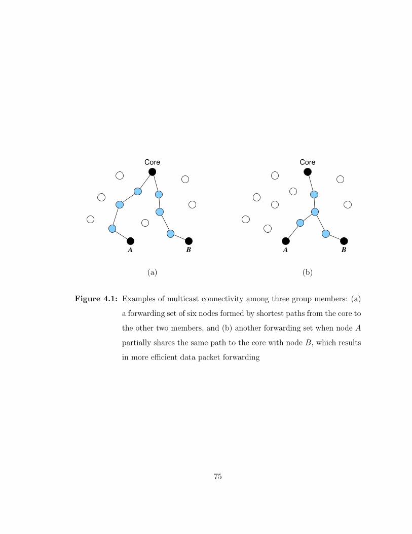
B
Core
A B
Core
A
(a) (b)
Figure 4.1: Examples of multicast connectivity among three group members: (a)
a forwarding set of six nodes formed by shortest paths from the core to
the other two members, and (b) another forwarding set when node A
partially shares the same path to the core with node B, which results
in more efficient data packet forwarding
75

Table 4.1: A few variations of the multicast routing problem and how each node
would compute its cost in MANSI
Problem Cost calculation per node
Load balancing Current traffic load or the current queue size
Power-aware routing Node’s transmission power
Energy conservation Inverse of the remaining energy of the node
Secure routing Security risk of the area the node is located in
the cost associated with each node can represent different measurements, depending
on the desired properties of the forwarding set. For instance, if we aim to reduce
the number of nodes in the forwarding set for efficient data forwarding, the cost
associated with each node could be one. Table 4.1 lists a few more examples of
what node cost would represent when MANSI is applied to other variations of the
multicast routing problem in wireless ad hoc networks.
We adopt the swarm intelligence metaphor to allow nodes to learn a better
multicast connection that yields a lower (total) forwarding cost. Each member who
is not the core periodically deploys a small packet, called a Forward Ant, that
opportunistically explores different, and hopefully better paths toward the core. This
exploring process is illustrated in Figure 4.2. If a Forward Ant arrives at a node
who is currently serving as a forwarding node for the group (node D in this case),
the ant turns itself into a Backward Ant and travels back to its originator via
the reverse path. When the Backward Ant arrives at each intermediate node, it
estimates the cost of having the node it is currently at join the forwarding set via the
forwarding node it previously found. The computed cost, as well as a pheromone
amount that is inversely proportional to the cost, are updated on the node’s local
data structure. These pheromone amounts are then used by subsequent Forward
76
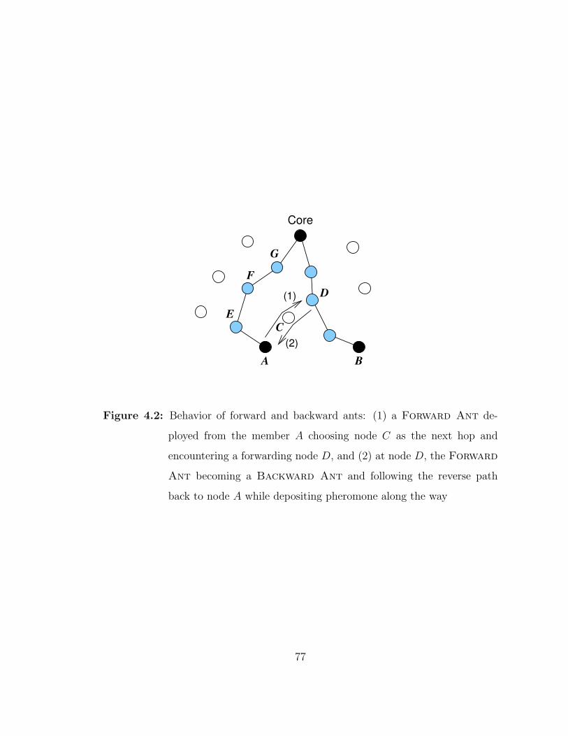
Core
BA
D
C(2)
(1)
E
F
G
Figure 4.2: Behavior of forward and backward ants: (1) a Forward Ant de-
ployed from the member A choosing node C as the next hop and
encountering a forwarding node D, and (2) at node D, the Forward
Ant becoming a Backward Ant and following the reverse path
back to node A while depositing pheromone along the way
77

id=3
id=6 id=8
h=3
h=6
h=6
h=8
h=8
h=8
h=∞h=6
Core
Figure 4.3: An example illustrating how heights are assigned to forwarding nodes
used by the members with IDs 3, 6 and 8
Ants that arrive at this node to make a decision which node they will travel to
next, similar to how pheromone is used by biological ants. Let us consider the same
example shown in Figure 4.2, when the Backward Ant leaves node D and arrives
at node C, the cost of having node C join the forwarding set via node D is zero since
node D is already a forwarding node and is directly connected to node C. When
the ant comes back to node A, the cost of having node A join the forwarding set
via node D is the same as the cost associated with node C because node C would
be required to become a forwarding node to allow node A to join the group via
node D. If node A sees that the pheromone amount on the link to node C becomes
the highest among links to all neighboring nodes, it will switch to join the group
via node C by sending a Join Request to node C. Consequently, node C will
become a forwarding node, while nodes E, F , and G will remove themselves from
the forwarding set (since they no longer hear requests from node A), which is similar
to the connectivity shown in Figure 4.1(b).
To prevent the race condition where members attempt to establish group
connectivity via one another’s forwarding path and nobody remains connected to
78
the core, each forwarding node is associated with a height which is identical to the
highest ID of the nodes that use it to connect to the core. In addition, the core
has its height set to infinity. Figure 4.3 shows an example illustrating how heights
are assigned to forwarding nodes. A Forward Ant must stop and turn into a
Backward Ant only when it encounters a forwarding node whose height is higher
than the ID of the member who originated the ant. That means a member is allowed
to connect to the core via an existing path that belongs to another member with a
higher ID, but not vice versa, to assure that the core, whose height is always the
highest, will eventually be connected to all the other members.
By following these simple rules, a majority of Forward Ants from each
member will choose a path that connects to an existing forwarding node with a
smaller total path cost. Nodes on this path are then used to forward multicast
data packets, resulting in a lower data forwarding cost. This exploring and learning
mechanism enables MANSI to learn a better forwarding set for each group, depend-
ing on how node cost is defined, as well as differentiates MANSI from other existing
ad hoc multicast routing protocols. Note that, by doing so, MANSI attempts to
evolve multicast connectivity into states that yield lower cost. It, however, does not
guarantee that minimum-cost connectivity can be achieved.
4.2 MANSI Protocol Description
4.2.1 Local Data Structures
Each node in the network is assigned a unique ID. A node with a unique ID
i maintains a list of neighboring nodes, ntab(i), obtained via a neighbor discovery
protocol such as periodic hello messaging. The node cost associated with node i
is denoted by cost(i), where cost(i) ≥ 0, which should be appropriately defined
to reflect the performance metric subject to minimization. In addition, for each
multicast group g, MANSI maintains the following data structures at each node i.
79

• Join table: maintains a list of nodes that have requested to join a multicast
group via node i. The join table of node i for multicast group g is denoted by
joing(i). This table is updated when node i hears a Join Request packet
intended to itself. Each entry in joing(i) is of the form 〈r, hr〉, where r is a
requesting node’s ID and hr is its height (as described in Section 4.1) that
it has sent along with its Join Request. The join table is initially empty
for each node. Node i becomes a forwarding node of the group g as long as
joing(i) 6= φ. When a neighbor j is removed from ntab(i) due to a link failure,
node i will remove all the corresponding entries 〈j, hj〉 from all the join tables.
• Core ID: denoted by coreg(i) to indicate the current core of group g. coreg(i)
is initially set to INVALID ADDRESS.
• Core sequence number: keeps track of the latest Core Announce’s se-
quence number, denoted by seqNog(i), and initially set to zero.
• Height: represents the height of node i if it is currently a member or a
forwarding node of the group g, defined as:
heightg(i) =
∞ if i = coreg(i)
max{i, max{hr | 〈r, hr〉 ∈ joing(i)}} if node i is a member
of group g
max{hr | 〈r, hr〉 ∈ joing(i)} otherwise.
(4.1)
As described in Section 4.1, the height of node i is the highest ID of the nodes,
including node i itself if it is a member, that are using node i to connect to
the core, and the core has an infinite height.
• Pheromone table: maps neighboring nodes and heights to pheromone in-
tensities. For node i, the pheromone intensity associated to the height h
80
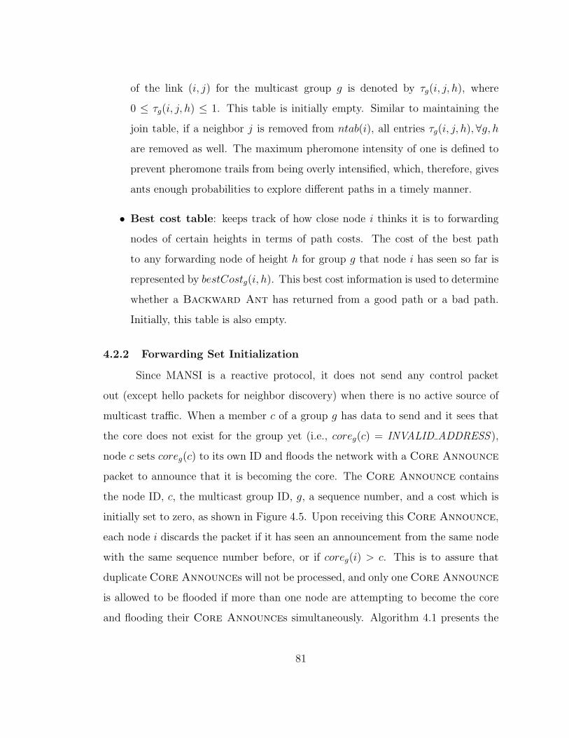
of the link (i, j) for the multicast group g is denoted by τg(i, j, h), where
0 ≤ τg(i, j, h) ≤ 1. This table is initially empty. Similar to maintaining the
join table, if a neighbor j is removed from ntab(i), all entries τg(i, j, h),∀g, h
are removed as well. The maximum pheromone intensity of one is defined to
prevent pheromone trails from being overly intensified, which, therefore, gives
ants enough probabilities to explore different paths in a timely manner.
• Best cost table: keeps track of how close node i thinks it is to forwarding
nodes of certain heights in terms of path costs. The cost of the best path
to any forwarding node of height h for group g that node i has seen so far is
represented by bestCostg(i, h). This best cost information is used to determine
whether a Backward Ant has returned from a good path or a bad path.
Initially, this table is also empty.
4.2.2 Forwarding Set Initialization
Since MANSI is a reactive protocol, it does not send any control packet
out (except hello packets for neighbor discovery) when there is no active source of
multicast traffic. When a member c of a group g has data to send and it sees that
the core does not exist for the group yet (i.e., coreg(c) = INVALID ADDRESS ),
node c sets coreg(c) to its own ID and floods the network with a Core Announce
packet to announce that it is becoming the core. The Core Announce contains
the node ID, c, the multicast group ID, g, a sequence number, and a cost which is
initially set to zero, as shown in Figure 4.5. Upon receiving this Core Announce,
each node i discards the packet if it has seen an announcement from the same node
with the same sequence number before, or if coreg(i) > c. This is to assure that
duplicate Core Announces will not be processed, and only one Core Announce
is allowed to be flooded if more than one node are attempting to become the core
and flooding their Core Announces simultaneously. Algorithm 4.1 presents the
81
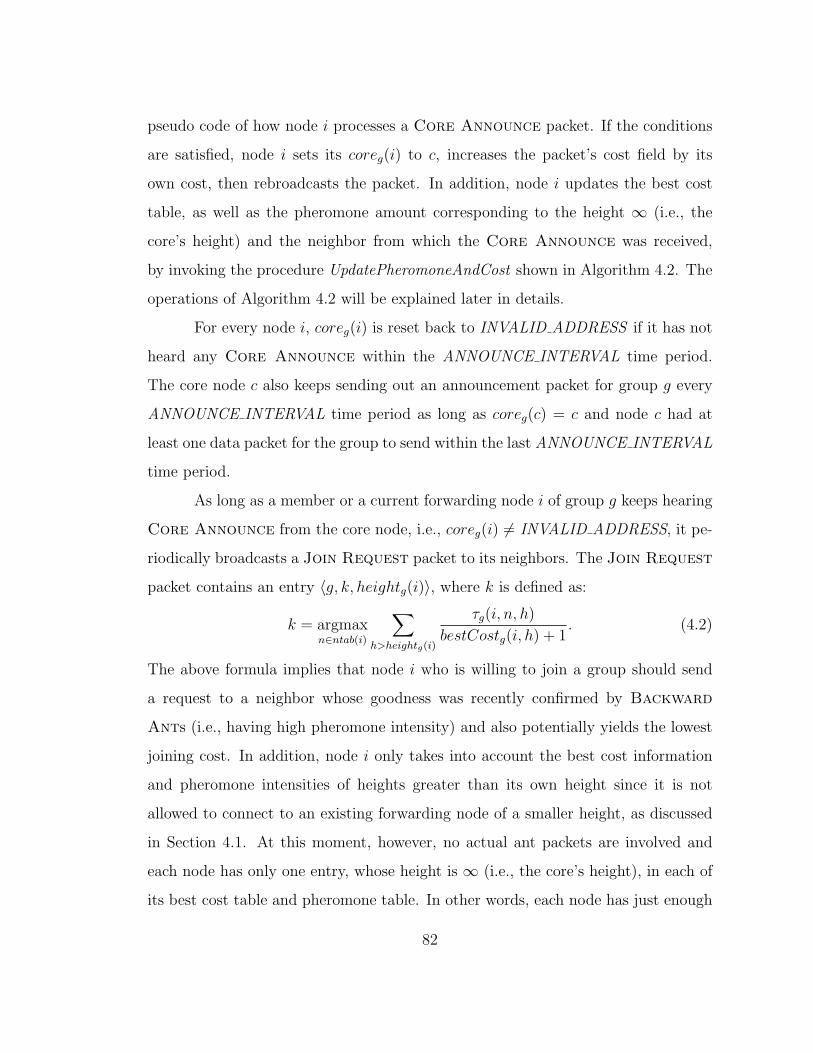
pseudo code of how node i processes a Core Announce packet. If the conditions
are satisfied, node i sets its coreg(i) to c, increases the packet’s cost field by its
own cost, then rebroadcasts the packet. In addition, node i updates the best cost
table, as well as the pheromone amount corresponding to the height ∞ (i.e., the
core’s height) and the neighbor from which the Core Announce was received,
by invoking the procedure UpdatePheromoneAndCost shown in Algorithm 4.2. The
operations of Algorithm 4.2 will be explained later in details.
For every node i, coreg(i) is reset back to INVALID ADDRESS if it has not
heard any Core Announce within the ANNOUNCE INTERVAL time period.
The core node c also keeps sending out an announcement packet for group g every
ANNOUNCE INTERVAL time period as long as coreg(c) = c and node c had at
least one data packet for the group to send within the last ANNOUNCE INTERVAL
time period.
As long as a member or a current forwarding node i of group g keeps hearing
Core Announce from the core node, i.e., coreg(i) 6= INVALID ADDRESS, it pe-
riodically broadcasts a Join Request packet to its neighbors. The Join Request
packet contains an entry 〈g, k, heightg(i)〉, where k is defined as:
k = argmaxn∈ntab(i)
∑h>heightg(i)
τg(i, n, h)
bestCostg(i, h) + 1. (4.2)
The above formula implies that node i who is willing to join a group should send
a request to a neighbor whose goodness was recently confirmed by Backward
Ants (i.e., having high pheromone intensity) and also potentially yields the lowest
joining cost. In addition, node i only takes into account the best cost information
and pheromone intensities of heights greater than its own height since it is not
allowed to connect to an existing forwarding node of a smaller height, as discussed
in Section 4.1. At this moment, however, no actual ant packets are involved and
each node has only one entry, whose height is ∞ (i.e., the core’s height), in each of
its best cost table and pheromone table. In other words, each node has just enough
82
1
47
50
(a)
1
47
50
(b)
Figure 4.4: Sample network snapshots illustrating the operations of MANSI: (a)
network setup with three members: nodes 1 (lower-left), 47 (upper-
right), and 50 (upper-left), where node 1 is the core, (b) dissemination
of Core Announce indicated by arrows
83

1
47
50
(c)
1
47
50
(d)
Figure 4.4: (cont’d) (c) initial multicast connectivity using reverse paths to the
core, resulting in a forwarding set of ten nodes (shown in gray), and
(d) forwarding set of four nodes learned by ants later in time
84
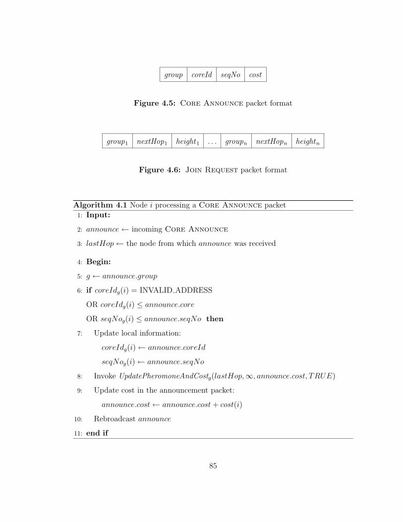
group coreId seqNo cost
Figure 4.5: Core Announce packet format
group1 nextHop1 height1 . . . groupn nextHopn heightn
Figure 4.6: Join Request packet format
Algorithm 4.1 Node i processing a Core Announce packet1: Input:
2: announce← incoming Core Announce
3: lastHop← the node from which announce was received
4: Begin:
5: g ← announce.group
6: if coreIdg(i) = INVALID ADDRESS
OR coreIdg(i) ≤ announce.core
OR seqNog(i) ≤ announce.seqNo then
7: Update local information:
coreIdg(i)← announce.coreId
seqNog(i)← announce.seqNo
8: Invoke UpdatePheromoneAndCostg(lastHop,∞, announce.cost, TRUE)
9: Update cost in the announcement packet:
announce.cost← announce.cost + cost(i)
10: Rebroadcast announce
11: end if
85

Algorithm 4.2 Procedure UpdatePheromoneAndCostg(next, height, cost, detF lag)
executed by node i1: Parameters:
2: next← neighbor ID indicating which pheromone table entry to be updated
3: height← height associated with this update
4: cost ← cost of joining the group g at a forwarding node of height height via
next
5: detF lag ← flag indicating whether this update is deterministic
6: Begin:
7: if τg(i, next, height) is not defined then
8: τg(i, next, height)← 0
9: end if
10: if detF lag = TRUE then
11: bestCostg(i, height)← cost
12: τg(i, next, height)← τg(i, next, height) + 12(1+cost)
13: else
14: if bestCostg(i, height) is not defined OR cost < bestCostg(i, height) then
15: bestCostg(i, height)← cost
16: τg(i, next, height)← 1 /* set intensity to max */
17: else
18: τg(i, next, height)← τg(i, next, height) + 11+cost
19: end if
20: end if
21: τg(i, next, height) ← min{τg(i, next, height), 1)} /* pheromone intensity is at
most one */
86
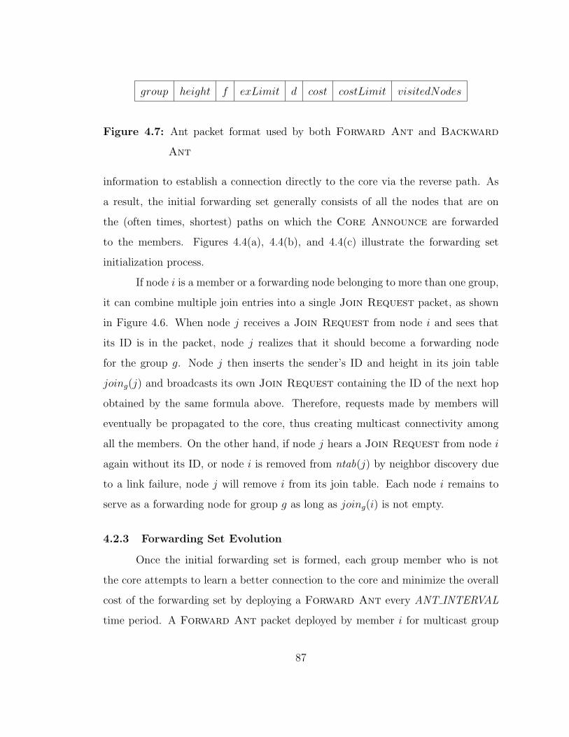
group height f exLimit d cost costLimit visitedNodes
Figure 4.7: Ant packet format used by both Forward Ant and Backward
Ant
information to establish a connection directly to the core via the reverse path. As
a result, the initial forwarding set generally consists of all the nodes that are on
the (often times, shortest) paths on which the Core Announce are forwarded
to the members. Figures 4.4(a), 4.4(b), and 4.4(c) illustrate the forwarding set
initialization process.
If node i is a member or a forwarding node belonging to more than one group,
it can combine multiple join entries into a single Join Request packet, as shown
in Figure 4.6. When node j receives a Join Request from node i and sees that
its ID is in the packet, node j realizes that it should become a forwarding node
for the group g. Node j then inserts the sender’s ID and height in its join table
joing(j) and broadcasts its own Join Request containing the ID of the next hop
obtained by the same formula above. Therefore, requests made by members will
eventually be propagated to the core, thus creating multicast connectivity among
all the members. On the other hand, if node j hears a Join Request from node i
again without its ID, or node i is removed from ntab(j) by neighbor discovery due
to a link failure, node j will remove i from its join table. Each node i remains to
serve as a forwarding node for group g as long as joing(i) is not empty.
4.2.3 Forwarding Set Evolution
Once the initial forwarding set is formed, each group member who is not
the core attempts to learn a better connection to the core and minimize the overall
cost of the forwarding set by deploying a Forward Ant every ANT INTERVAL
time period. A Forward Ant packet deployed by member i for multicast group
87

g, whose format is shown in Figure 4.7, contains the following fields:
• group: multicast group ID
• height: height of the forwarding node found by this ant. This field is used
only after this ant has been turned to a Backward Ant.
• f : forwarding flag indicating whether this ant is a Forward Ant or a Back-
ward Ant (since they share the same structure). Since node i is deploying a
Forward Ant, this flag is set to TRUE.
• exLimit: the number of times the ant is allowed to probabilistically pick a
next hop that is not the current best one to prevent it from aimlessly traversing
the network. This field is initially set to EXPLORE LIMIT and decrements
every time the ant makes a decision on a next hop probabilistically, instead of
deterministically choosing the next hop given by (4.2).
• d: deterministic flag indicating whether the ant should always follow the cur-
rent best path and obtain the actual current cost for the best cost table. The
reason for using deterministic ants is that costs in the best cost table may no
longer reflect the actual costs due to node mobility, dynamics of nodes’ costs,
or dynamics of the forwarding set itself. If this flag is set, the exLimit field is
always ignored. Every other ant deployed by each member is deterministic.
• cost: the total cost of the nodes this ant has visited, initially set to zero.
• costLimit: the cost limit of the path that the ant is allowed to traverse after
leaving its originator. This field is used in conjunction with the cost field to
prevent the ant from traversing forward after the accumulated cost exceeds
the limit. Usually this limit is set to minh>i bestCostg(i, h), i.e., the lowest
known cost to a current forwarding node of group g that node i is allowed to
88
connect to, plus some threshold. By this way, the ant can stop proceeding
once it is certain that it will not find any better path than what its originator
currently has. This cost limit is ignored if the ant is deterministic since its
goal is not to find a better cost, but to find the actual current best cost.
• visitedNodes: the set of nodes visited by the ant, initially set to {i}.
A node deploying a Forward Ant invokes the procedure ReleaseForwar-
dAnt described in Algorithm 4.3 to find the next hop that the ant will travel to. A
desirability, defined in (4.3), is computed for each of the neighboring nodes by giving
higher values to neighbors that have higher pheromone intensities and potentially
yield lower costs to connect to an existing forwarding node. On the other hand, zero
desirability is given to all the nodes that have been visited before. If the ant is not
deterministic and is still allowed to explore, these desirabilities are then normalized
to obtain a probability of choosing each of the neighboring nodes. Otherwise the
neighbor node that gives the maximum desirability is chosen, which has the same
effect as using (4.2) except that it excludes all the nodes in the visitedNodes field.
Once a next hop is chosen, its ID is appended to the end of visitedNodes and the
ant is broadcast.
When a node j receives a Forward Ant, it checks if its ID matches the ID at
the end of the ant’s visitedNodes field. If not, the ant is discarded. Otherwise, node
j knows that this ant is intended to itself and accepts it. Algorithm 4.4 shows how
a Forward Ant is processed. First, node j checks if it is currently a forwarding
node of the group and its height is higher than the ID of the ant’s originator. If so,
node j realizes that the member who deployed the ant is eligible to join the group
via node j itself. This ant is then turned into a Backward Ant by resetting its
f flag. The ant’s cost field is then reset to zero to start computing the total cost
on the way back, and its height field is set to node j’s height. The last entry of the
ant’s visitedNodes is removed in order to send this ant back to the previous hop.
89

Algorithm 4.3 Procedure ReleaseForwardAntg(fant) executed by node i
1: Parameter:
2: fant← a Forward Ant to be released
3: Begin:
4: Compute a desirability, dn, for node n, n ∈ ntab(i) from summations of only
entries whose heights are higher than fant.height in the main pheromone table:
dn =
0 if n ∈ fant.visitedNodes
1 +∑
h>fant.heightτg(i,n,h)
bestCostg(i,h)+1if τg(i, n, h) exists
1 otherwise.
(4.3)
5: if ∀n, dn = 0 then
6: return /* ant has no place to go */
7: end if
8: If fant is not deterministic (fant.d = FALSE) and it is allowed to explore
(fant.exLimit > 0), with probability 0.5, fant decides to randomly choose a
next hop n, where the probably of choosing n depends on its desirability as
follows:
Prob(n) =dn∑
k∈ntab(i) dk
(4.4)
fant.exLimit← fant.exLimit−1 /* ant just performs one more exploration
*/
9: Otherwise, the next hop is set to the one whose desirability is maximum:
n← argmaxk∈ntab(i) dk
10: append n to fant.visitedNodes and broadcast fant
90

Algorithm 4.4 Node i processing a Forward Ant packet1: Input:
2: fant← incoming Forward Ant
3: Begin:
4: if i = last entry in fant.visitedNodes then
5: g ← fant.group
6: if joing(i) 6= φ AND fant.visitedNodes[0] < heightg(i) then
7: Convert fant to a Backward Ant
fant.cost← 0
fant.height← heightg(i)
fant.f ← FALSE
8: Remove last entry from fant.visitedNodes and broadcast fant
9: else
10: fant.cost← fant.cost + cost(i)
11: if fant.cost < fant.costLimit OR fant.d = TRUE then
12: Invoke ReleaseForwardAntg(fant)
13: end if
14: end if
15: end if
91

If the condition is not satisfied to convert the ant to a Backward Ant,
node j increases the ant’s cost field by its own cost, cost(j). Node j then invokes
the procedure ReleaseForwardAnt to forward the ant to a next hop, as long as the
updated cost does not exceed the limit or the ant is deterministic.
Algorithm 4.5 Node i processing a Backward Ant packet1: Input:
2: bant← incoming Backward Ant
3: lastHop← the node from which bant was received
4: Begin:
5: g ← fant.group
6: Invoke UpdatePheromoneAndCostg(lastHop, bant.height, bant.cost, bant.d)
7: if i = last entry in fant.visitedNodes then
8: Remove the last entry from bant.visitedNodes
9: if bant.visitedNodes 6= φ then
10: bant.cost← bant.cost + cost(i)
11: broadcast bant
12: end if
13: end if
When a node k hears a Backward Ant from node j, it invokes the pro-
cedure UpdatePheromoneAndCost, described in Algorithm 4.2, which updates the
entries in node k’s pheromone and best cost tables in accordance with node j and
the height field. If the ant is deterministic, the cost that the ant carries back is the
actual cost of the path its originator is currently using to join the group. Therefore,
the best cost corresponding to the height field is updated to this value. If the ant
is not deterministic, however, the best cost is updated only when it is higher than
the returned cost, which means that the ant has found a better path to join the
group from this node. The pheromone intensity on this link is also updated to the
92

maximum to encourage subsequent Forward Ants to use the same link, as well
as to redirect join request to this link instead. If the ant comes back with a higher
cost, a pheromone amount of 1/(1 + cost) is added instead. In case of deterministic
ant, the added amount is reduced by half since this link already has the highest
pheromone intensity as it has just been chosen by a deterministic Forward Ant.
Note that we have mentioned this procedure before when we explained how a node
uses it while processing a Core Announce (line 8 of Algorithm 4.1). This is be-
cause a Core Announce more or less serves as a deterministic Backward Ant
returning from the core.
After updating the pheromone and the best cost tables, node k checks if
the Backward Ant was intended to itself by examining the last entry in the ant’s
visitedNodes field. If its ID matches, node k adds its cost into the cost field, removes
the last entry from visitedNodes, and rebroadcasts as long as there is at least one
entry left in visitedNodes. Algorithm 4.5 presents the pseudo code of how a node
processes a Backward Ant.
Similar to pheromone evaporation of biological ants, each node i updates all
the entries τg(i, j, h) in its pheromone table by reducing their values by DECAY-
ING FACTOR at every DECAY INTERVAL time period:
τg(i, j, h) = (1− DECAYING FACTOR)× τg(i, j, h), (4.5)
where 0 < DECAYING FACTOR < 1.
By probabilistically selecting next hops, the majority of the Forward Ants
will choose paths with high pheromone intensity, while some of them may explore
totally different new paths. If a Backward Ant comes back with a better cost on
a new branch, the pheromone amount on that branch will be increased significantly.
As a result, a change in multicast connectivity (i.e., forwarding set) is triggered due
to the periodic broadcast of Join Request packets, as illustrated in Figure 4.4(d).
93
MANSI also takes advantage of broadcast nature of wireless communication
to speed up the learning process as follows. When node i overhears a Join Request
for group g from node j but not intended to itself, it invokes UpdatePheromone-
AndCostg(j, hj, 0, TRUE), where hj is the height that node j reports in its Join
Request. This implies that node i could join the group via node j with no cost,
given that its height is less than hj. However, a drawback of this idea is that some
members who are not forwarding nodes will broadcast Join Requests as well and
might be mistaken as forwarding nodes by its neighbors.
4.2.4 Multicast Data Forwarding
Since MANSI is a mesh-based protocol which allows forwarding nodes and
members to accept data packets arriving from any node, each data packet is assigned
a unique sequence number when it is transmitted from the source. The sequence
numbers are checked by each forwarding node and member node to make sure that no
duplicate data packets are rebroadcast or delivered to the application. When node
i receives a non-duplicate data packet of group g, it checks whether it is currently
a forwarding node of the group, i.e., joing(i) 6= φ. If so, node i rebroadcasts the
packet. Otherwise, the packet is silently discarded.
4.2.5 Handling Mobility
In MANSI, mobility and other network dynamics are handled inherently
rather than as exceptions. With the pheromone laying/following behavior of Back-
ward Ants and Forward Ants, each path comprising the forwarding set keeps
being reinforced as long as no link on the path is broken. However, network dy-
namics can cause optimal connectivity to change from time to time even though the
current connectivity may still be valid. With the probabilistic nature of Forward
Ants to explore new paths, the multicast forwarding set should be able to evolve
into a configuration that is more efficient for the new topology.
94
When a link currently used by a member or a forwarding node to send Join
Requests breaks, the pheromone table entries corresponding to that link are also
removed. Therefore, all subsequent Forward Ants will be redirect to other paths,
while the majority of them will take the next hop whose pheromone intensity was
the second highest before the link failure. If this next hop leads to a forwarding
node of a higher height, Backward Ants will return and update pheromone on
the new path, hence reestablishing a connection to the group. However, in case that
Forward Ants fail to find a new path, periodically flooding of Core Announces
will eventually restore the connectivity.
Although MANSI is considered a mesh-based protocol by its way of forward-
ing data packets, connectivity of the forwarding set may still be fragile if the network
is sparse and members are far apart from each other, especially with the presence of
mobility. To make data forwarding more effective under mobility, while maintain-
ing good efficiency when the network is static, we incorporate a mobility-adaptive
mechanism into MANSI. This mechanism requires nodes to compute the normalized
link failure frequency, or nlff , by keeping track of link failures detected from their
neighbors. MANSI uses the same calculation of nlff as used by ADBM, which are
shown in equations (3.1) and (3.2). Each member or forwarding node then uses this
nlff to determine the stability of its surrounding area. If its nlff is lower than a
threshold NLFF THRESHOLD, the node will consider its area stable and join the
group by sending Join Requests toward its best next hop as usual. If nlff exceeds
the threshold, however, the node will add another entry for the second best next hop
into its Join Requests. Since all the neighbors are ranked by their goodness in
terms of pheromone intensities, the second best next hop can be easily determined.
Formally, if node k is the best next hop for node i to join the group g, as defined in
(4.2), then the second best next hop k′ is defined as:
k′ = argmaxn∈ntab(i),n6=k
∑h>heightg(i)
τg(i, n, h)
bestCostg(i, h) + 1. (4.6)
95
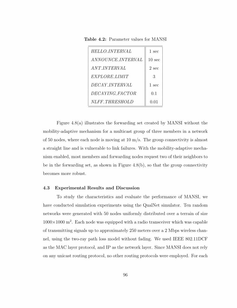
Table 4.2: Parameter values for MANSI
HELLO INTERVAL 1 sec
ANNOUNCE INTERVAL 10 sec
ANT INTERVAL 2 sec
EXPLORE LIMIT 3
DECAY INTERVAL 1 sec
DECAYING FACTOR 0.1
NLFF THRESHOLD 0.01
Figure 4.8(a) illustrates the forwarding set created by MANSI without the
mobility-adaptive mechanism for a multicast group of three members in a network
of 50 nodes, where each node is moving at 10 m/s. The group connectivity is almost
a straight line and is vulnerable to link failures. With the mobility-adaptive mecha-
nism enabled, most members and forwarding nodes request two of their neighbors to
be in the forwarding set, as shown in Figure 4.8(b), so that the group connectivity
becomes more robust.
4.3 Experimental Results and Discussion
To study the characteristics and evaluate the performance of MANSI, we
have conducted simulation experiments using the QualNet simulator. Ten random
networks were generated with 50 nodes uniformly distributed over a terrain of size
1000×1000 m2. Each node was equipped with a radio transceiver which was capable
of transmitting signals up to approximately 250 meters over a 2 Mbps wireless chan-
nel, using the two-ray path loss model without fading. We used IEEE 802.11DCF
as the MAC layer protocol, and IP as the network layer. Since MANSI does not rely
on any unicast routing protocol, no other routing protocols were employed. For each
96
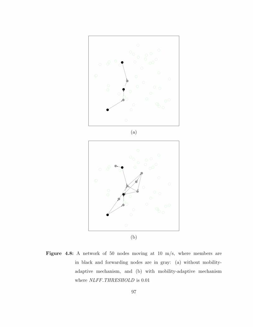
(a)
(b)
Figure 4.8: A network of 50 nodes moving at 10 m/s, where members are
in black and forwarding nodes are in gray: (a) without mobility-
adaptive mechanism, and (b) with mobility-adaptive mechanism
where NLFF THRESHOLD is 0.01
97
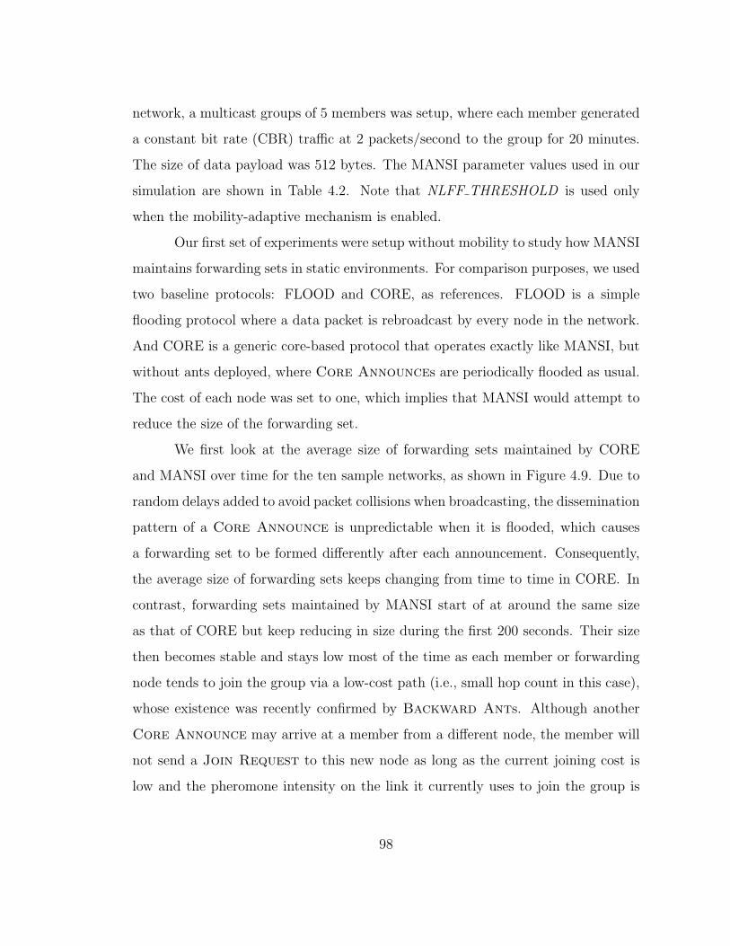
network, a multicast groups of 5 members was setup, where each member generated
a constant bit rate (CBR) traffic at 2 packets/second to the group for 20 minutes.
The size of data payload was 512 bytes. The MANSI parameter values used in our
simulation are shown in Table 4.2. Note that NLFF THRESHOLD is used only
when the mobility-adaptive mechanism is enabled.
Our first set of experiments were setup without mobility to study how MANSI
maintains forwarding sets in static environments. For comparison purposes, we used
two baseline protocols: FLOOD and CORE, as references. FLOOD is a simple
flooding protocol where a data packet is rebroadcast by every node in the network.
And CORE is a generic core-based protocol that operates exactly like MANSI, but
without ants deployed, where Core Announces are periodically flooded as usual.
The cost of each node was set to one, which implies that MANSI would attempt to
reduce the size of the forwarding set.
We first look at the average size of forwarding sets maintained by CORE
and MANSI over time for the ten sample networks, as shown in Figure 4.9. Due to
random delays added to avoid packet collisions when broadcasting, the dissemination
pattern of a Core Announce is unpredictable when it is flooded, which causes
a forwarding set to be formed differently after each announcement. Consequently,
the average size of forwarding sets keeps changing from time to time in CORE. In
contrast, forwarding sets maintained by MANSI start of at around the same size
as that of CORE but keep reducing in size during the first 200 seconds. Their size
then becomes stable and stays low most of the time as each member or forwarding
node tends to join the group via a low-cost path (i.e., small hop count in this case),
whose existence was recently confirmed by Backward Ants. Although another
Core Announce may arrive at a member from a different node, the member will
not send a Join Request to this new node as long as the current joining cost is
low and the pheromone intensity on the link it currently uses to join the group is
98
0
1
2
3
4
5
6
7
8
0 200 400 600 800 1000
#nod
es in
the
forw
ardi
ng s
et
Simulation time (s)
COREMANSI
Figure 4.9: Average size of the forwarding set as a function of time for CORE and
MANSI
99

Table 4.3: Average size of the forwarding set formed in MANSI, CORE, and
FLOOD for each network
Average SizeNetwork
MANSI CORE FLOOD
1 7.9 9.5 50.0
2 4.0 3.7 50.0
3 4.0 5.0 50.0
4 4.5 4.7 50.0
5 6.5 8.5 50.0
6 5.5 6.3 50.0
7 6.9 7.8 50.0
8 6.0 7.5 50.0
9 5.2 7.7 50.0
10 5.0 7.0 50.0
Average 5.6 6.7 50.0
100
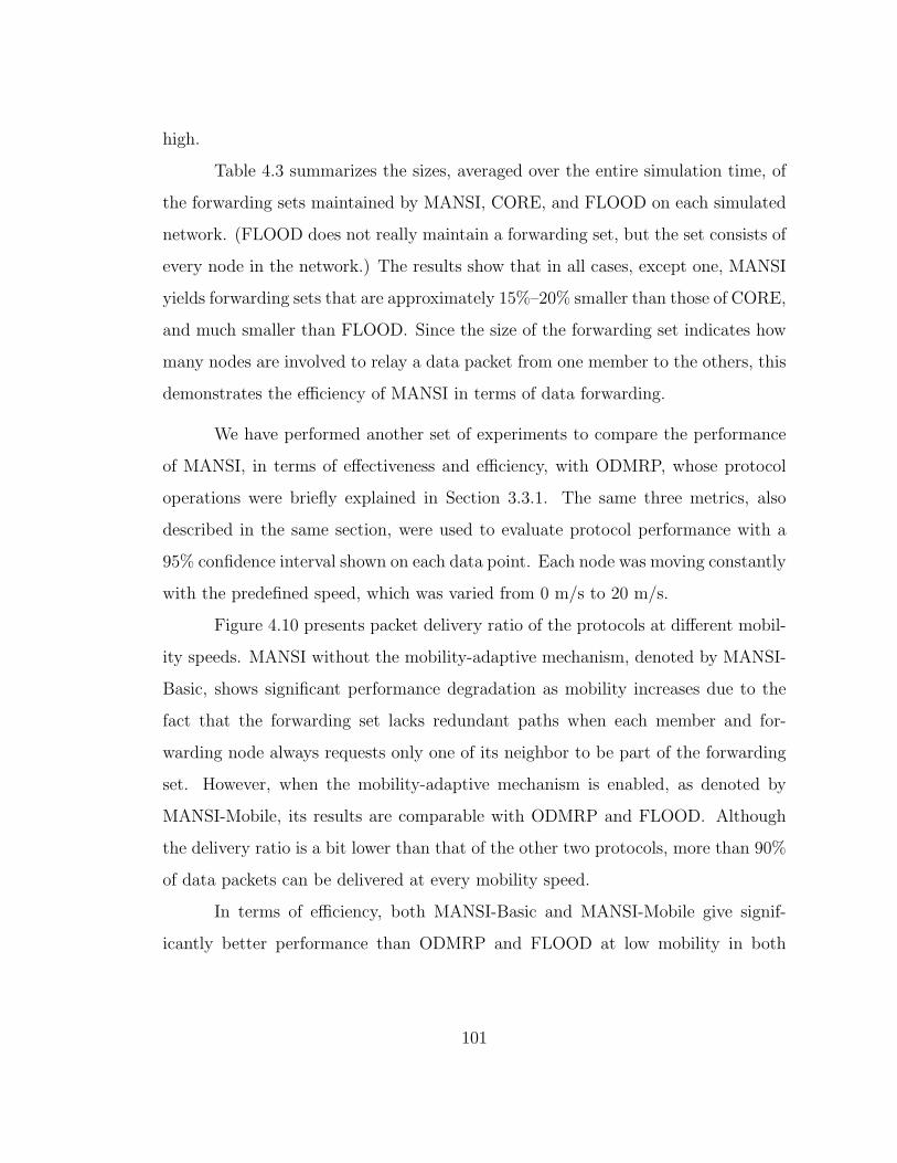
high.
Table 4.3 summarizes the sizes, averaged over the entire simulation time, of
the forwarding sets maintained by MANSI, CORE, and FLOOD on each simulated
network. (FLOOD does not really maintain a forwarding set, but the set consists of
every node in the network.) The results show that in all cases, except one, MANSI
yields forwarding sets that are approximately 15%–20% smaller than those of CORE,
and much smaller than FLOOD. Since the size of the forwarding set indicates how
many nodes are involved to relay a data packet from one member to the others, this
demonstrates the efficiency of MANSI in terms of data forwarding.
We have performed another set of experiments to compare the performance
of MANSI, in terms of effectiveness and efficiency, with ODMRP, whose protocol
operations were briefly explained in Section 3.3.1. The same three metrics, also
described in the same section, were used to evaluate protocol performance with a
95% confidence interval shown on each data point. Each node was moving constantly
with the predefined speed, which was varied from 0 m/s to 20 m/s.
Figure 4.10 presents packet delivery ratio of the protocols at different mobil-
ity speeds. MANSI without the mobility-adaptive mechanism, denoted by MANSI-
Basic, shows significant performance degradation as mobility increases due to the
fact that the forwarding set lacks redundant paths when each member and for-
warding node always requests only one of its neighbor to be part of the forwarding
set. However, when the mobility-adaptive mechanism is enabled, as denoted by
MANSI-Mobile, its results are comparable with ODMRP and FLOOD. Although
the delivery ratio is a bit lower than that of the other two protocols, more than 90%
of data packets can be delivered at every mobility speed.
In terms of efficiency, both MANSI-Basic and MANSI-Mobile give signif-
icantly better performance than ODMRP and FLOOD at low mobility in both
101
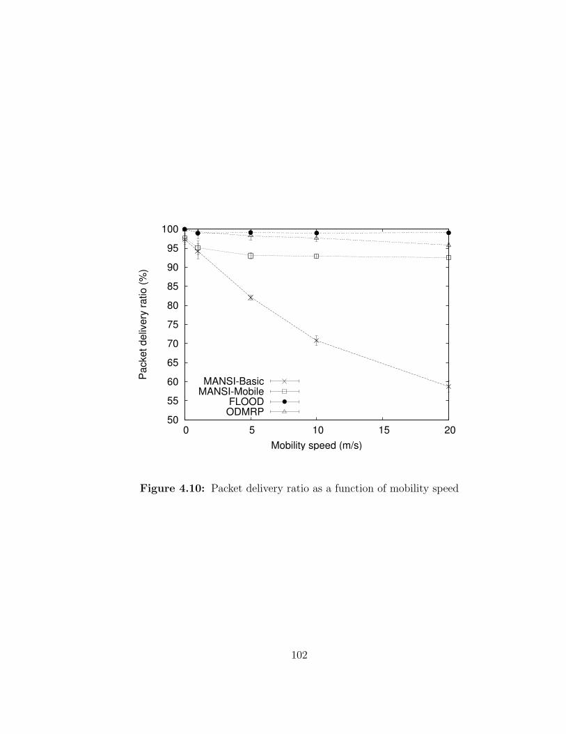
50
55
60
65
70
75
80
85
90
95
100
0 5 10 15 20
Pac
ket d
eliv
ery
ratio
(%)
Mobility speed (m/s)
MANSI-BasicMANSI-Mobile
FLOODODMRP
Figure 4.10: Packet delivery ratio as a function of mobility speed
102
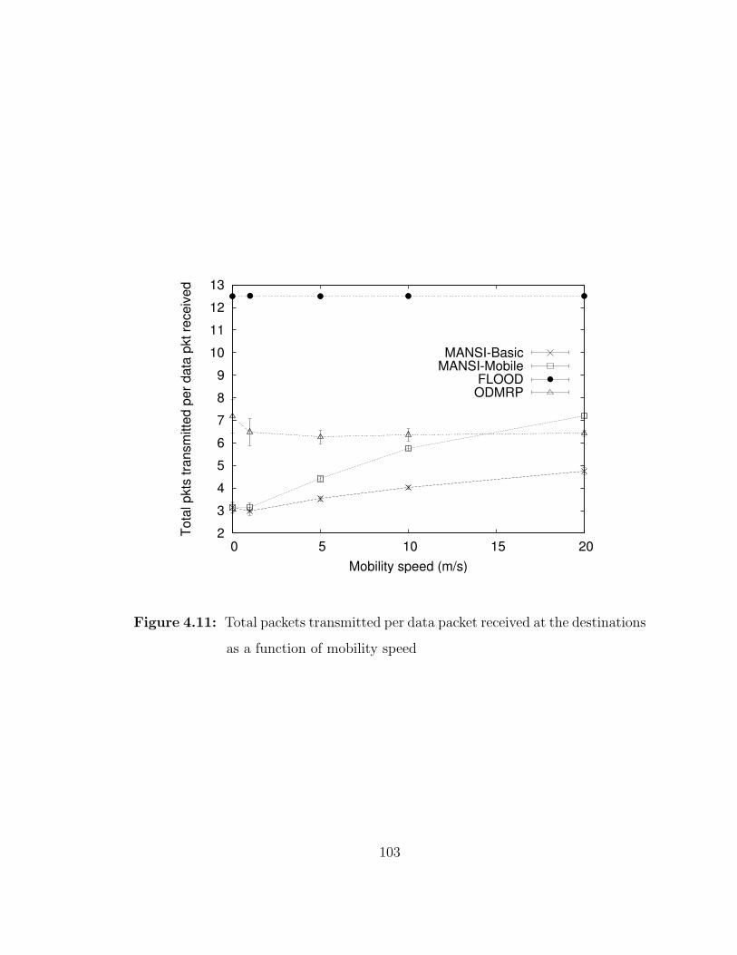
2
3
4
5
6
7
8
9
10
11
12
13
0 5 10 15 20
Tota
l pkt
s tra
nsm
itted
per
dat
a pk
t rec
eive
d
Mobility speed (m/s)
MANSI-BasicMANSI-Mobile
FLOODODMRP
Figure 4.11: Total packets transmitted per data packet received at the destinations
as a function of mobility speed
103
0
2
4
6
8
10
12
14
0 5 10 15 20Tota
l byt
es tr
ansm
itted
per
dat
a by
te re
ceiv
ed
Mobility speed (m/s)
MANSI-BasicMANSI-Mobile
FLOODODMRP
Figure 4.12: Total bytes transmitted per data byte received at the destinations as
a function of mobility speed
104
channel access and bandwidth utilization aspects, as shown in Figure 4.11 and Fig-
ure 4.12, respectively. The reason is that every multicast sender floods Join Query
packets periodically in ODMRP, while in MANSI, only the core of the group per-
forms periodic flooding. Moreover, ODMRP requires each member to send a Join
Reply toward each sender via the reverse path on which the Join Query was
received, resulting in a fairly large forwarding group, especially with high number
of senders. MANSI, in contrast, has each member establish connectivity toward the
core, which keeps the number of forwarding nodes low.
Without adapting their behaviors to mobility, data forwarding characteris-
tics of MANSI-Basic, ODMRP, and FLOOD remain almost the same regardless of
mobility speeds, where FLOOD employs the highest number of forwarding nodes,
and MANSI-Basic uses the least number, but suffers low packet delivery ratio under
high mobility. With its mobility-adaptive mechanism, MANSI-Mobile is shown to
perform as efficiently as MANSI-Basic at low mobility1 and as ODMRP at high
mobility, while yielding consistently high packet delivery ratio for the entire range
of mobility speeds.
4.4 Summary
Inspired by swarm intelligence, we have introduced an alternative approach
to solving the multicast routing problem in mobile ad hoc networks. The protocol,
called MANSI (Multicast for Ad hoc Networks with Swarm Intelligence), is an on-
demand multicast routing protocol that creates a multicast mesh shared by all the
members within each group. The protocol uses a core-based scheme, where each
member initiates a request to the core node to establish multicast connectivity with
other members. Intermediate nodes who receive such a request become forwarding
1 In fact, they behave exactly the same
105
nodes that are used to relay data packets from one member to the others. Un-
like other core-based protocols, MANSI does not always rely on the shortest paths
between the core and the members to establish group connectivity. Instead, each
member who is not the core periodically deploys a small packet that behaves like an
ant to opportunistically explore different paths. This exploring mechanism enables
the protocol to discover paths that comprise a better set of forwarding nodes yield-
ing a lower total cost of data forwarding, where the “cost” of forwarding (nodes) can
be defined in terms of different application specific performance metrics. MANSI
also incorporates a mobility-adaptive mechanism that allows the protocol to remain
effective as mobility increases. The simulation results have shown that MANSI per-
forms both effectively and efficiently in static or low-mobility environments, yet still
effectively in highly dynamic environments.
106
Chapter 5
A FRAMEWORK FOR EVOLUTIONARY MULTICAST
ROUTING
Due to their efficient utilization of network bandwidth, reactive routing pro-
tocols, both unicast and multicast, are often preferable to proactive protocols. How-
ever, since a source obtains a route to the destination(s) on demand in a reactive
protocol, the amount of effort in acquiring the route determines how quickly the
route can be found, and how efficient it is. We observe there are two different as-
pects concerning the efficiency of reactive routing protocols: (1) efficiency of the
connectivity establishment process, and (2) efficiency of the connectivity itself. For
instance, a flooding protocol, which requires every node to forward data packets, uses
the entire network as the connectivity between the source and the destination(s).
Hence, it requires no effort to establish the connectivity (since the connectivity is
the entire network) and is considered the most efficient from the connectivity estab-
lishment aspect. However, flooding’s connectivity is most inefficient because data
forwarding involves every single node in the network. On the contrary, protocols
that attempt to establish the optimal connectivity such as finding a shortest route
(for unicast) or a minimum set of forwarding nodes (for multicast) usually result in
a large amount of control overhead to obtain the route in a short period of time.
The process of establishing optimal connectivity is therefore considered inefficient.
107
To help design and evaluate reactive multicast routing protocols that can
achieve efficiency in both aspects, we introduce the Evolutionary Multicast Routing
Framework (EMRF) for mobile ad hoc networks.
5.1 Evolutionary Multicast Routing Framework (EMRF)
EMRF provides a generic framework that decomposes the multicast routing
process in mobile ad hoc networks into two phases: a forwarding set initialization
and a forwarding set evolution. By using different mechanisms for the two phases,
various protocol instances can be created. These protocols should be able to quickly
and efficiently establish initial multicast connectivity, then refine the resulting con-
nectivity via different optimization techniques. Within EMRF, MANSI, as described
in Chapter 4, is a protocol instance that uses (1) flooding to extract a forwarding
set for the initialization phase, and (2) swarm intelligence to adapt the forwarding
set for the forwarding set evolution phase.
Phase 1: Forwarding Set Initialization
This phase is responsible for reactively constructing an initial forwarding set,
preferably in a quick and efficient way. This process could be initiated by the first
member who has data to be sent to other group members. For the consistency of the
terminology used in this dissertation, this node will be referred to as the core of the
group, meaning that it will be serving as the focal point for all other group members.
Recall from the previous chapter on MANSI, the core initiates the construction of an
initial forwarding set by distributing an announcement packet to all other members
so that these members can request intermediate nodes along the reverse paths to
form a forwarding set. Within EMRF, the distribution of announcement packets is
carried out by a connected subset of nodes, called an announcement set, which is
assumed to be available a priori. For a multicast group g, its current announcement
set is denoted as ASg. Applicable techniques for determining an announcement set
108

to be used to distribute announcement packets to all the group members include,
but not limited to, the following:
• Flooding – every node in the network belongs to ASg for any multicast group
g. As long as the network is not partitioned, all the members will receive this
announcement. This technique, therefore, is the most robust and needs no
underlying infrastructure, but can potentially causes a scalability problem due
to large amount of bandwidth usage.
• Virtual backbone – as mentioned in Section 2.1.2, virtual backbones such
as connected dominating sets provide a solution to avoiding global flooding.
In this framework, these backbone infrastructures are used to disseminate
announcement packets from the core. If a backbone is constructed based on a
connected dominating set (where each node is either a backbone node or an
immediate neighbor of one), ASg will consist of every node on the backbone
for any group g. In contrast, if the backbone construction algorithm allows
backbone nodes to have more than one hop coverage, a node i who joins
a group g will be responsible for informing its associated backbone node a
priori. In this case, all intermediate nodes on the path between node i and
the associated backbone node will also belong to ASg.
• Leader election – leader election protocols [MWV00] allow nodes to elect a
single node to act as the leader for the entire network. To establish multicast
connectivity, the leader can serve as a rendezvous point through which nodes
can join a multicast group and disseminate multicast traffic (similar to CBT).
Therefore, for a multicast group g, ASg consists of every intermediate node on
the path between each group member and the leader, plus the leader itself.
Once an announcement is initiated, the forwarding set construction process
is similar to what is used in MANSI. A member of the multicast group g or any
109
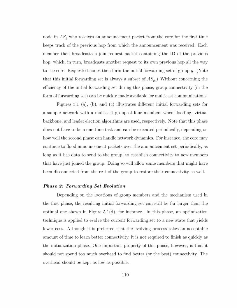
node in ASg who receives an announcement packet from the core for the first time
keeps track of the previous hop from which the announcement was received. Each
member then broadcasts a join request packet containing the ID of the previous
hop, which, in turn, broadcasts another request to its own previous hop all the way
to the core. Requested nodes then form the initial forwarding set of group g. (Note
that this initial forwarding set is always a subset of ASg.) Without concerning the
efficiency of the initial forwarding set during this phase, group connectivity (in the
form of forwarding set) can be quickly made available for multicast communications.
Figures 5.1 (a), (b), and (c) illustrates different initial forwarding sets for
a sample network with a multicast group of four members when flooding, virtual
backbone, and leader election algorithms are used, respectively. Note that this phase
does not have to be a one-time task and can be executed periodically, depending on
how well the second phase can handle network dynamics. For instance, the core may
continue to flood announcement packets over the announcement set periodically, as
long as it has data to send to the group, to establish connectivity to new members
that have just joined the group. Doing so will allow some members that might have
been disconnected from the rest of the group to restore their connectivity as well.
Phase 2: Forwarding Set Evolution
Depending on the locations of group members and the mechanism used in
the first phase, the resulting initial forwarding set can still be far larger than the
optimal one shown in Figure 5.1(d), for instance. In this phase, an optimization
technique is applied to evolve the current forwarding set to a new state that yields
lower cost. Although it is preferred that the evolving process takes an acceptable
amount of time to learn better connectivity, it is not required to finish as quickly as
the initialization phase. One important property of this phase, however, is that it
should not spend too much overhead to find better (or the best) connectivity. The
overhead should be kept as low as possible.
110
Network leader
Regular node
Backbone node
������Multicast group member Virtual backbone
Initial group connectivity
Backbone/leader node associativity
Sender
������
������
������
������
Sender
������
������
������
������
(a) (b)
Sender
������
������
������
������
Sender
������
������
������
������
(c) (d)
Figure 5.1: Illustrations of initial multicast connectivity for four group members
using different underlying infrastructures: (a) no infrastructure (i.e.,
simple flooding), incurring a forwarding set of 8 nodes, (b) virtual
backbone, also resulting in 8 forwarding nodes, (c) single leader, result-
ing in 9 forwarding nodes, and (d) the optimal connectivity, requiring
only 5 forwarding nodes
111
According to the desired properties of this phase discussed above, various
optimization techniques can be used. An example of such techniques is the swarm
intelligence based mechanism employed by MANSI in the previous chapter where
each member deploys packets that act like biological ants to explore and learn
new forwarding sets with lower overall cost. Self-stabilization [Dij74], as used in
[GS99a, GBS00, GS03] where each node simply exchanges periodic messages with
its neighboring nodes to achieve global objectives in constructing a multicast tree,
is also applicable. Note that some optimization techniques, such as MANSI, are
based on heuristics which may not guarantee global optimization (i.e., finding the
minimum forwarding set). This phase, therefore, may or may not evolve the initial
forwarding sets illustrated in Figures 5.1(a)-(c) into a similar (optimal) result shown
in Figure 5.1(d).
Based on this framework, short multicast sessions can quickly establish group
connectivity in the first phase, but may not benefit from the second phase which
requires some time to converge. However, since established connectivity will be
used for only a short period of time, optimality of the forwarding sets is not the
main concern. In contrast, the second phase should be beneficial for long-running
multicast sessions, where nodes in the forwarding set are required to forward packets
for an extended period of time. According to these operations described above,
MANSI can now be considered an instance of EMRF, where the forwarding set
initialization employs a global flooding technique and a swarm intelligence based
technique is used in the forwarding set evolution phase.
5.2 Case Study: Integration of ADBM and MANSI
To demonstrate EMRF, we integrate the backbone construction mechanism
of ADBM with the swarm intelligence (SI) based evolution mechanism of MANSI,
112

explained in Chapter 3 and Chapter 4, respectively, and introduce a protocol in-
stance of EMRF called ADBM/SI. The backbone construction mechanism of ADBM
sets up the virtual infrastructure to serve as an announcement set, which is used
in place of flooding in MANSI, for constructing an initial forwarding set. The SI
based exploring and learning mechanisms of MANSI are then used for forwarding
set evolution. In this integration, every node functions in the same way as required
by ADBM, except when forwarding data packets. Multicast connectivity for a group
g that was used in ADBM becomes the announcement set ASg. Formally, a node
i belongs to ASg as long as node i meets one of the three conditions described in
Section 3.2.2. The first member who has data to be sent to the group floods a
Core Announce packet over ASg to trigger the forwarding set formation, and
continues flooding Core Announces as long as it still has data to send. When a
node i receives a Core Announce packet, the node executes Algorithm 5.1, which
is adapted from Algorithm 4.1 used in MANSI (note the difference in lines 8 and
10–12). Since Core Announces are carried over a backbone and are not likely
traveling on a shortest path between the core and node i, the pheromone updat-
ing rule for Core Announces should follow the rule for nondeterministic ants.
Hence the last parameter used in the invocation of UpdatePheromoneAndCost is
set to FALSE instead. Procedures of updating pheromone, releasing forward ants,
and processing forward and backward ants remain the same, which are shown in
Algorithms 4.2, 4.3, 4.4, and 4.5, respectively.
5.3 Experimental Results and Discussion
We studied the performance of the ADBM/SI protocol via simulation using
QualNet. The simulation environment is the same as what we use in MANSI, as
described in Section 4.3. Parameters used in the ADBM portion and SI portion
of the protocol are also taken from the experiments on the original protocols listed
113
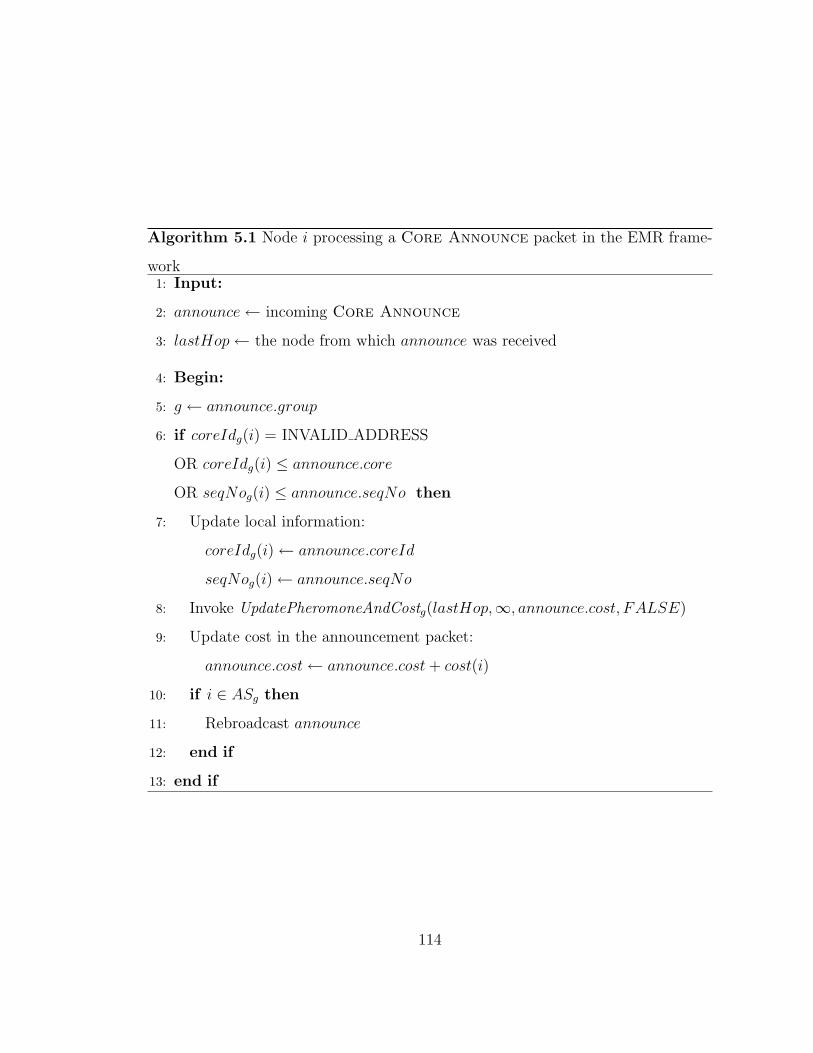
Algorithm 5.1 Node i processing a Core Announce packet in the EMR frame-
work1: Input:
2: announce← incoming Core Announce
3: lastHop← the node from which announce was received
4: Begin:
5: g ← announce.group
6: if coreIdg(i) = INVALID ADDRESS
OR coreIdg(i) ≤ announce.core
OR seqNog(i) ≤ announce.seqNo then
7: Update local information:
coreIdg(i)← announce.coreId
seqNog(i)← announce.seqNo
8: Invoke UpdatePheromoneAndCostg(lastHop,∞, announce.cost, FALSE)
9: Update cost in the announcement packet:
announce.cost← announce.cost + cost(i)
10: if i ∈ ASg then
11: Rebroadcast announce
12: end if
13: end if
114
in Table 3.5 and Table 4.2, respectively. Table 5.1 summarizes the network and
protocol parameter settings.
The first set of results, presented in Table 5.2, compare the average size of
non-evolvable forwarding sets (denoted by |FSg| w/o ants) and evolvable forwarding
sets (denoted by |FSg| w/ ants), including the average size of announcement sets
(|ASg|), in static environments. The left three columns are the results when flooding
is used to distribute Core Announces, i.e., all the 50 nodes are in ASg, which
is similar to MANSI described in the previous chapter. Results in the right three
columns are collected when ASg is determined by ADBM, which involves about
40% of nodes on average. We can observe from the table that using a backbone
as an announcement set may result in either larger and smaller initial forwarding
sets compared to those obtained by flooding. Larger initial forwarding sets can be
created, since reverse paths from members to the core are limited to only nodes on
the backbone. On the other hand, smaller forwarding sets are also possible because
less nodes in the announcement set give higher chances for members to share the
same path back to the core. However, both flooding and ADBM result in evolvable
forwarding sets of approximately 10% smaller than their non-evolvable forms on
average, while ADBM ends up with slightly smaller forwarding sets when they are
allowed to evolve. Note that the final forwarding sets are expected to be even smaller
since their sizes shown in Table 5.2 are averaged over the entire simulation time.
We now compare the performance of ADBM and MANSI versus the inte-
grated ADBM/SI on the application aspect. The same three metrics described in
Section 3.3.1 are used here to show the effectiveness and the efficiency of delivering
packets to members by each protocol. Figure 5.2 compares packet delivery ratio at
mobility speeds 0, 5, 10, and 20 m/s. When the network is static, ADBM, MANSI,
and ADBM/SI have very small differences in delivering packets. As mobility in-
creases, drops in packet delivery ratio can be observed from 0 m/s to 5 m/s in all
115
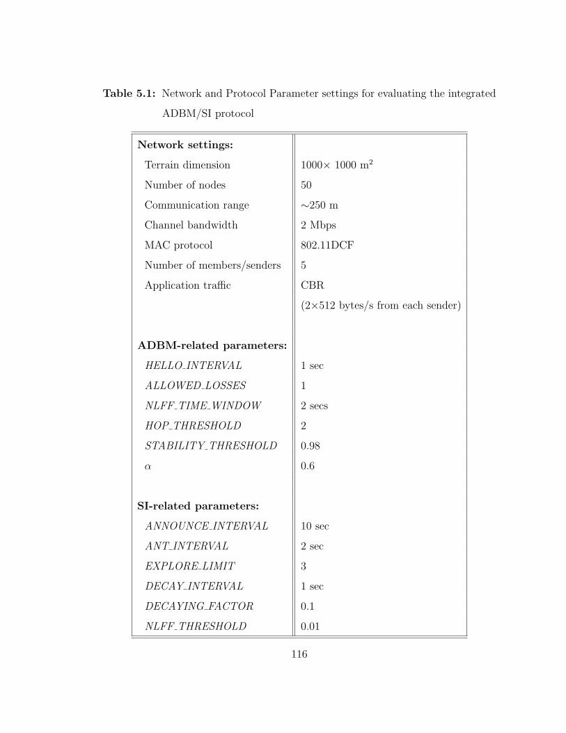
Table 5.1: Network and Protocol Parameter settings for evaluating the integrated
ADBM/SI protocol
Network settings:
Terrain dimension 1000× 1000 m2
Number of nodes 50
Communication range ∼250 m
Channel bandwidth 2 Mbps
MAC protocol 802.11DCF
Number of members/senders 5
Application traffic CBR
(2×512 bytes/s from each sender)
ADBM-related parameters:
HELLO INTERVAL 1 sec
ALLOWED LOSSES 1
NLFF TIME WINDOW 2 secs
HOP THRESHOLD 2
STABILITY THRESHOLD 0.98
α 0.6
SI-related parameters:
ANNOUNCE INTERVAL 10 sec
ANT INTERVAL 2 sec
EXPLORE LIMIT 3
DECAY INTERVAL 1 sec
DECAYING FACTOR 0.1
NLFF THRESHOLD 0.01
116
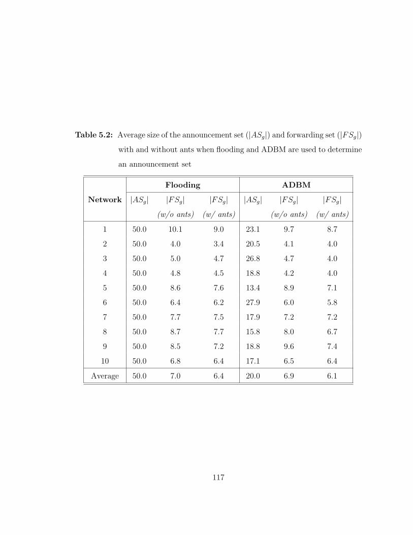
Table 5.2: Average size of the announcement set (|ASg|) and forwarding set (|FSg|)
with and without ants when flooding and ADBM are used to determine
an announcement set
Flooding ADBM
Network |ASg| |FSg| |FSg| |ASg| |FSg| |FSg|
(w/o ants) (w/ ants) (w/o ants) (w/ ants)
1 50.0 10.1 9.0 23.1 9.7 8.7
2 50.0 4.0 3.4 20.5 4.1 4.0
3 50.0 5.0 4.7 26.8 4.7 4.0
4 50.0 4.8 4.5 18.8 4.2 4.0
5 50.0 8.6 7.6 13.4 8.9 7.1
6 50.0 6.4 6.2 27.9 6.0 5.8
7 50.0 7.7 7.5 17.9 7.2 7.2
8 50.0 8.7 7.7 15.8 8.0 6.7
9 50.0 8.5 7.2 18.8 9.6 7.4
10 50.0 6.8 6.4 17.1 6.5 6.4
Average 50.0 7.0 6.4 20.0 6.9 6.1
117
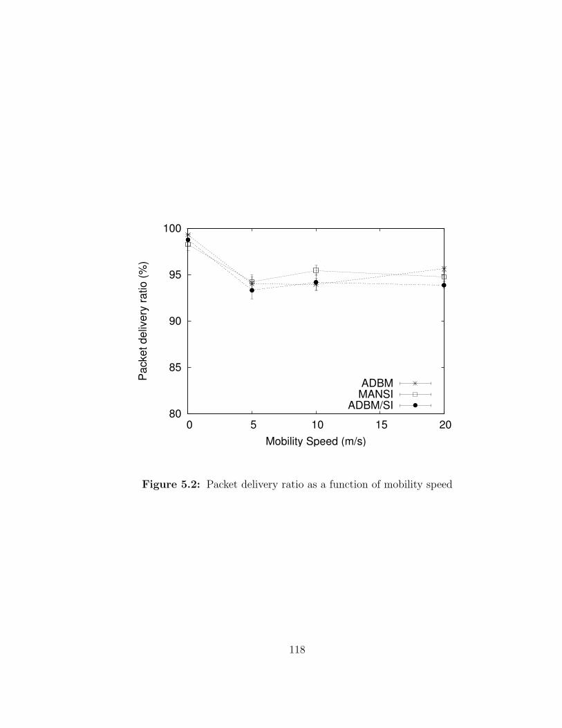
80
85
90
95
100
0 5 10 15 20
Pac
ket d
eliv
ery
ratio
(%)
Mobility Speed (m/s)
ADBMMANSI
ADBM/SI
Figure 5.2: Packet delivery ratio as a function of mobility speed
118

0
1
2
3
4
5
6
7
8
9
0 5 10 15 20Tota
l pkt
s tra
nsm
itted
per
dat
a pk
t rec
eive
d
Mobility Speed (m/s)
ADBMMANSI
ADBM/SI
Figure 5.3: Total packets transmitted per data packet received at the destinations
as a function of mobility speed
119
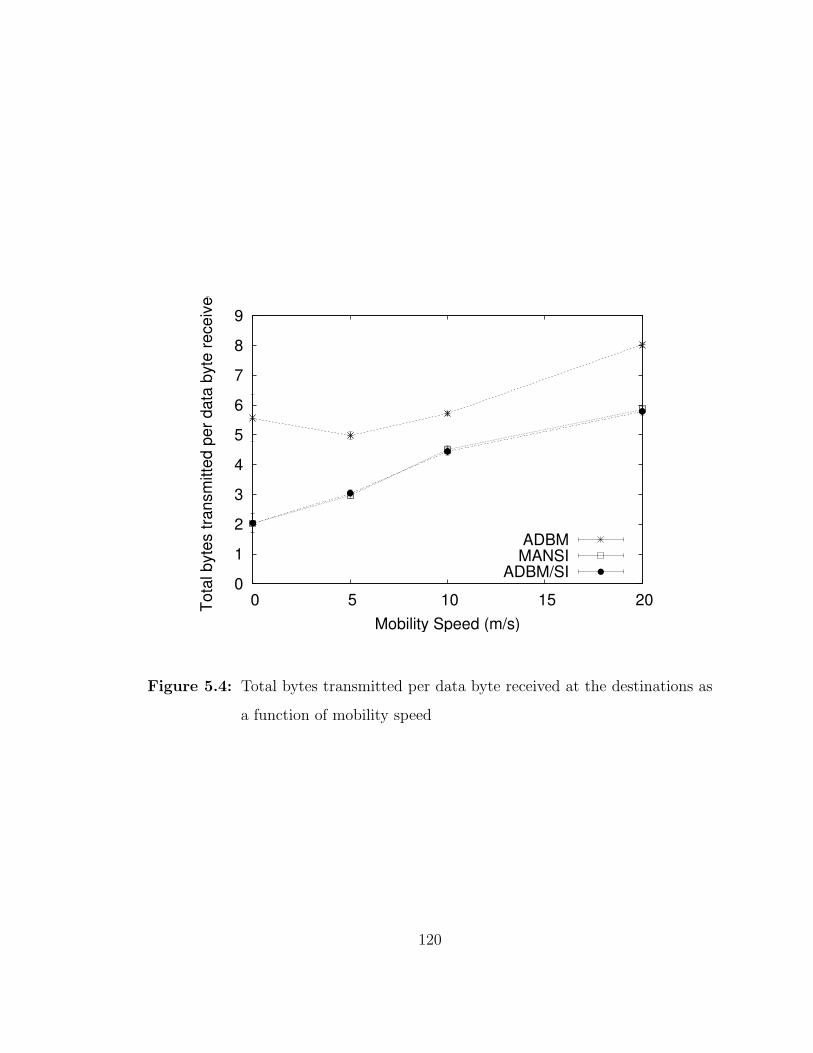
0
1
2
3
4
5
6
7
8
9
0 5 10 15 20Tota
l byt
es tr
ansm
itted
per
dat
a by
te re
ceiv
ed
Mobility Speed (m/s)
ADBMMANSI
ADBM/SI
Figure 5.4: Total bytes transmitted per data byte received at the destinations as
a function of mobility speed
120
the protocols and becomes steady at higher speeds since all the protocols incorpo-
rate a mobility-adaptive mechanism that induces more nodes to serve as forwarding
nodes. However, ADBM/SI yields slightly lower delivery ratio than the other two
due to the fact that it relies on a backbone to distribute Core Announce pack-
ets. Although ADBM tries to be responsive to mobility by maintaining the stability
constraints (which reduces the coverage area of each backbone node), it still does
not guarantee that the backbone will stay connected 100% of the time. If the back-
bone becomes disconnected at the moment the core broadcasts a Core Announce,
connectivity may not be refreshed for some members whose connections to the core
have broken and not yet been restored by ants.
In terms of efficiency, as presented in Figure 5.3 and Figure 5.4, ADBM
has the highest overhead due to the use of more forwarding nodes (i.e., the en-
tire backbone). MANSI and ADBM/SI are equally efficient in both packets and
bytes transmitted. However, a slightly lower number of total packets transmitted
(i.e., slightly higher efficiency) can be observed from ADBM/SI because the use of
backbones can help avoid network-wide flooding of Core Announce packets.
5.4 Summary
This chapter has described the evolutionary multicast routing framework, or
EMRF for short, for mobile ad hoc networks. Within EMRF, the multicast routing
process in mobile ad hoc networks is divided into a forwarding set initialization phase
and a forwarding set evolution phase. EMRF allows independent incorporation of
different mechanisms for the two phases to create protocol instances that can quickly
and efficiently establish initial multicast connectivity and/or effectively improve the
resulting connectivity via different optimization techniques. To demonstrate EMRF,
we presented a protocol that exploits a virtual backbone provided by ADBM as an
infrastructure to establish initial multicast connectivity without global flooding. A
swarm intelligence based technique is then used to evolve the connectivity to a
121

more efficient state. The new protocol is evaluated via simulation and is shown to
yield similar performance as the MANSI protocol. This gives us confidence that we
may be able to initialize multicast meshes using any existing virtual infrastructures,
based on network conditions and operational constraints, and have them evolve, by
way of swarm intelligence for instance, into similar and efficient states.
122
Chapter 6
MULTICAST WITH DIRECTIONAL ANTENNAS
In wireless communications, an antenna is the port through which radio fre-
quency (RF) energy is coupled from the transmitter to the environment, and re-
versely, to the receiver from the environment. The manner in which RF energy is
distributed into and collected from surrounding environments has a profound impact
on the efficient use of spectrum and the service quality provided. With the advance
in technology, directional antennas [HP96], which combine multiple antenna ele-
ments with signal-processing capability to control the radiation and/or reception
patterns in response to the environment, are emerging to facilitate spatial reuse,
high data rate, low probability of detection, robustness to jamming, and mobile
communications in highly dynamic environments.
Although a number of directional antenna-based MAC protocols have been
proposed [HS02, HSSJ02a, KSV00, NYH00, SGZ01], these protocols only investigate
the usage of directional antennas in unicast mode of communication. With direc-
tional antennas, when a signal transmitted by one node is expected to be received by
more than one neighboring nodes, especially in multicast routing, information from
upper-layer protocols is often required to determine an appropriate beam formation
of the broadcast signal. As part of our research on multicast routing for ad hoc
networks, we investigated the benefits and impacts of applying directional antennas
for multicast communications.
Intuitively, using directional antennas to direct transmitted signals to known
destinations would help reduce interference and increase overall network capacity
123
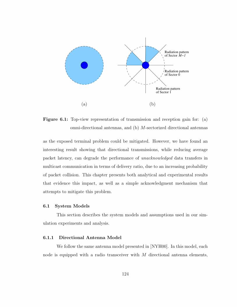
Radiation pattern
Radiation patternof Sector 1
of Sector 0
Radiation patternof Sector M−1
(a) (b)
Figure 6.1: Top-view representation of transmission and reception gain for: (a)
omni-directional antennas, and (b) M -sectorized directional antennas
as the exposed terminal problem could be mitigated. However, we have found an
interesting result showing that directional transmissions, while reducing average
packet latency, can degrade the performance of unacknowledged data transfers in
multicast communication in terms of delivery ratio, due to an increasing probability
of packet collision. This chapter presents both analytical and experimental results
that evidence this impact, as well as a simple acknowledgment mechanism that
attempts to mitigate this problem.
6.1 System Models
This section describes the system models and assumptions used in our sim-
ulation experiments and analysis.
6.1.1 Directional Antenna Model
We follow the same antenna model presented in [NYH00]. In this model, each
node is equipped with a radio transceiver with M directional antenna elements,
124

�����������
������ �� �����������
Figure 6.2: k out of M antenna sectors can be enabled simultaneously while trans-
mitting a multicast packet to multiple receivers located in different
sectors.
each of which spans an angle of 360/M degrees, as shown in Figure 6.1(b). All
nodes are assumed to share the same wireless channel. Each node maintains a fixed
orientation of its antenna element(s) at all time, regardless of its own orientation.
Upon receiving a signal, the node can also identify from which sector the signal is
received. In addition, the MAC protocol is capable of switching k antenna elements
on simultaneously, where 1 ≤ k ≤ M , which affects both signal transmission and
reception. This allows a multicast packet to be sent to multiple receivers located in
different sectors in a single transmission without interfering other nodes, as shown
in Figure 6.2. When all the M directions are on, the directional antenna has the
same characteristic as an omni-directional antenna. When a signal is transmitted,
the transmission power can be adjusted so that the transmission range in terms of
radial distance remains the same regardless of how many sectors are turned on.
6.1.2 Signal Transmission and Reception Model
As our main focus is to apply directional antennas to multicast communi-
cation, packet transmission for multicast packets is generally done in the broadcast
mode at the MAC layer. For many wireless MAC protocols such as IEEE 802.11,
125
transmissions in the broadcast mode is not guaranteed since the collision avoid-
ance and acknowledgment features are not employed.1 However, the carrier sensing
mechanism is still utilized. Our model, therefore, assumes no handshake or acknowl-
edgment of any kind.
During a single-hop communication, the sender and the receiver determine
their transmission and reception schemes independently. Since their antennas may
be set to be either omni-directional or directional, the sender/receiver pair can
operate in either of the following four modes:
1. Omni-directional Reception Omni-directional Transmission (OROT):
The sender always transmits a signal omni-directionally. While the signal is
being received, the receiver can still hear signals coming from other directions,
but these signals cannot be received and will be interpreted as interference.
This mode is similar to using traditional omni-directional antennas and is used
as the reference case.
2. Directional Reception Omni-directional Transmission (DROT): The
sender transmits a signal omni-directionally. However, the receiver is able to
lock the signal by turning on only the sector on which the signal is being
received. By this way, the reception is interfered only when there are other
signals coming from the same direction.
3. Omni-directional Reception Directional Transmission (ORDT): As-
suming the direction of the receiver is known, the sender can enable only the
sector within which the receiver is located. The receiver will leave its antenna
in the omni-directional mode while receiving a signal, so it can be interfered
by other signals heard from any direction.
1 In the case of IEEE 802.11, for example, this means RTS, CTS, and ACK framesare never used.
126
4. Directional Reception Directional Transmission (DRDT): Directional
mode is used in both transmission and reception. Similar to ORDT, the sender
is allowed to enable only the sector which corresponds to the location of the
receiver. The receiver then turns on only the sector necessary to receive the
signal to prevent interference from the other directions.
6.2 Preliminary Experiment
We first conducted a preliminary experiment using the QualNet to study
the behaviors and performance comparison of the four different modes (i.e., OROT,
DROT, ORDT and DRDT) in exploiting directional antennas for multicast commu-
nication. The experiment was performed on 30 random simulated networks, each
of which consisted of 50 stationary nodes uniformly distributed over a terrain of
size 1000×1000 m2. Each node was equipped with a radio transceiver with eight
directional antenna elements (M = 8). Regardless of the number of enabled antenna
elements, each transmission would cover a communication range of approximately
250 meters over a 2 Mbps wireless channel. The two-ray path loss model without
fading was assumed. We used IEEE 802.11DCF as the MAC layer protocol, and IP
as the network layer.
Only one multicast session was run with 25 group members randomly selected
from the 50 nodes. Group sources were then selected from the 25 members, each of
which was configured to generate a constant bit rate (CBR) traffic of 4 packets/s.
Each CBR packet contained a 512-byte payload. The number of sources was varied
from 1 to 20 and was used as the control variable in this experiment. ADBM, de-
scribed in Chapter 3, was used to provide the multicast service. Since the protocol
already requires each node to maintain a neighbor table to keep track of its cur-
rent neighboring nodes by means of beaconing, we extended this neighbor discover
mechanism to record the antenna direction to each of its neighbor to support ORDT
and DRDT modes. The direction information is obtained from the physical layer
127
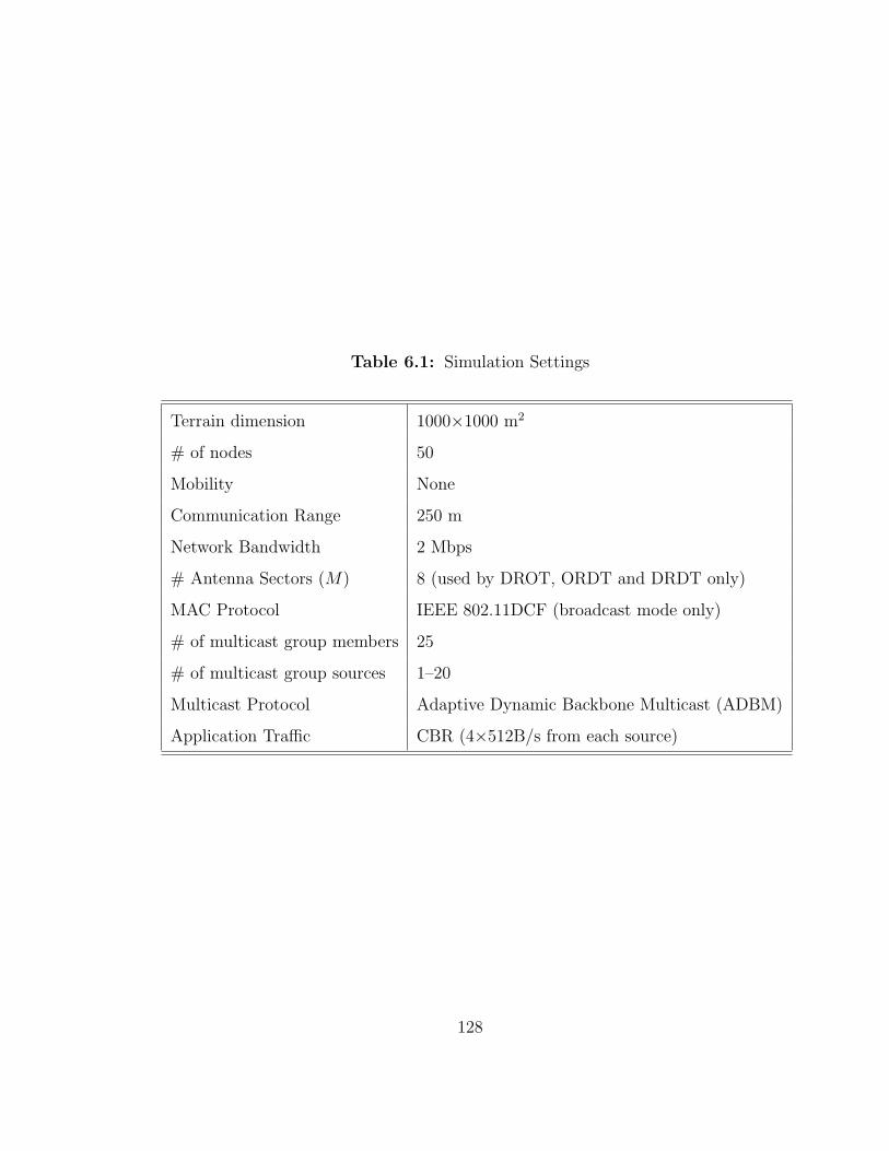
Table 6.1: Simulation Settings
Terrain dimension 1000×1000 m2
# of nodes 50
Mobility None
Communication Range 250 m
Network Bandwidth 2 Mbps
# Antenna Sectors (M) 8 (used by DROT, ORDT and DRDT only)
MAC Protocol IEEE 802.11DCF (broadcast mode only)
# of multicast group members 25
# of multicast group sources 1–20
Multicast Protocol Adaptive Dynamic Backbone Multicast (ADBM)
Application Traffic CBR (4×512B/s from each source)
128
by checking which antenna sector obtains the highest signal strength when a signal
is received from a neighbor. For each multicast group, each forwarder or member
also maintains a list of all the next-hop forwarders and members of the same group.
When a node is about to broadcast a data packet in ORDT or DRDT mode, it
combines this next-hop list with the direction information from the neighbor table
and passes the resulting antenna directions down to the physical layer so that only
antenna sectors corresponding to the next hops are enabled for that transmission.
Note that those four modes of communication described in the previous section are
generic and can be incorporated into any existing multicast protocols with slight
modification, if any. Although ADBM was chosen in this study for our convenience,
results from other multicast protocols would be relatively similar, as long as they
only rely on IEEE 802.11’s broadcast mode. We did not simulate node mobility
since different multicast protocols handle mobility differently and would not pro-
duce general results in our study. Table 6.1 summarizes the settings used in the
simulation experiments. Each data point presented in the results is shown with a
95% confidence interval.
The first result depicted in Figure 6.3 shows the average end-to-end delay
as a function of the number of sources under different communication modes. As
expected, using directional antennas to transmit signals (ORDT and DRDT modes)
helps reduce the average delay since other nodes close to a sending node can start
sending their signals right away without waiting for that node to complete its trans-
mission. This means that, to some extent, the exposed terminal problem is mit-
igated. The delay differences are not visible under low load conditions (less than
10 sources), but they become more significant as the load increases whereas the
network layer’s queues start to overflow. However, as we will see later, mitigation
of the exposed terminal problem is not the only reason directional transmissions
yield low delays, especially for ORDT. It can be observed that ORDT’s delays
129
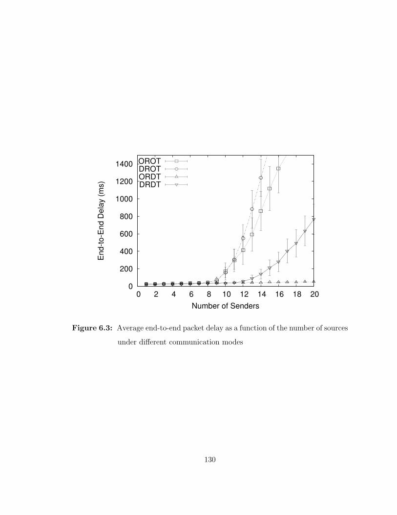
0
200
400
600
800
1000
1200
1400
0 2 4 6 8 10 12 14 16 18 20
End
-to-E
nd D
elay
(ms)
Number of Senders
OROTDROTORDTDRDT
Figure 6.3: Average end-to-end packet delay as a function of the number of sources
under different communication modes
130
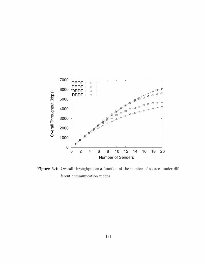
0
1000
2000
3000
4000
5000
6000
7000
0 2 4 6 8 10 12 14 16 18 20
Ove
rall
Thro
ughp
ut (k
bps)
Number of Senders
OROTDROTORDTDRDT
Figure 6.4: Overall throughput as a function of the number of sources under dif-
ferent communication modes
131
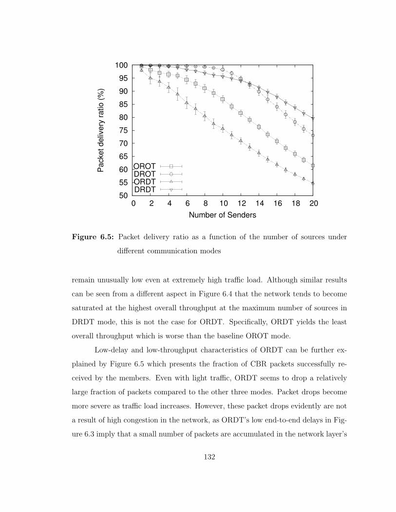
50
55
60
65
70
75
80
85
90
95
100
0 2 4 6 8 10 12 14 16 18 20
Pac
ket d
eliv
ery
ratio
(%)
Number of Senders
OROTDROTORDTDRDT
Figure 6.5: Packet delivery ratio as a function of the number of sources under
different communication modes
remain unusually low even at extremely high traffic load. Although similar results
can be seen from a different aspect in Figure 6.4 that the network tends to become
saturated at the highest overall throughput at the maximum number of sources in
DRDT mode, this is not the case for ORDT. Specifically, ORDT yields the least
overall throughput which is worse than the baseline OROT mode.
Low-delay and low-throughput characteristics of ORDT can be further ex-
plained by Figure 6.5 which presents the fraction of CBR packets successfully re-
ceived by the members. Even with light traffic, ORDT seems to drop a relatively
large fraction of packets compared to the other three modes. Packet drops become
more severe as traffic load increases. However, these packet drops evidently are not
a result of high congestion in the network, as ORDT’s low end-to-end delays in Fig-
ure 6.3 imply that a small number of packets are accumulated in the network layer’s
132

queues most of the time. Since there is no mobility in the network, these packet
losses are not caused by topology changes either. From the same graph, OROT also
drops many packets but it still performs significantly better than ORDT. Given
that signals transmitted directionally by ORDT would cause less interference and
give higher network capacity due to the use of narrower beams, these results are
counter-intuitive. Similar trends can be observed for DROT and DRDT. DROT
provides the most reliability in terms of packet delivery under light to moderate
traffic load (less than 10 sources), followed by DRDT. At high traffic loads, how-
ever, DRDT yields the best performance due to higher network capacity gained
from spatial reuse of directional antennas. Despite the lower average end-to-end de-
lay and the higher overall throughput, DRDT noticeably causes more packet drops
than DROT in moderate traffic conditions. If we look at Figure 6.3 again, it shows
that networks operating in OROT and DROT modes start getting congested around
9 sources, while DRDT starts suffering from congestion around 13 sources (while
ORDT suffers no congestion at all). In Figure 6.5, delivery ratio given by DRDT
is already lower than that of DROT when the number of sources is far below 13.
Similar to ORDT, these packet losses are definitely not due to congestion. There-
fore, there must be another problem behind the use of directional transmissions that
causes a noticeable fraction of packets to be dropped.
An explanation of this counter-intuitive behavior of directional transmissions
in fact can be evidenced by the physical layer and the operation of IEEE 802.11’s
broadcast mode. Figure 6.6 presents the number of collisions detected at the physical
layer for OROT, DROT, ORDT, and DRDT. The results show that operating in
ORDT and DRDT modes cause many more collisions than operating in OROT
and DROT modes, respectively. When a packet is dropped due to collisions, it is
simply lost and never gets retransmitted since IEEE 802.11’s broadcast mode does
not use acknowledgments. As a result, without congestion ORDT and DRDT give
133
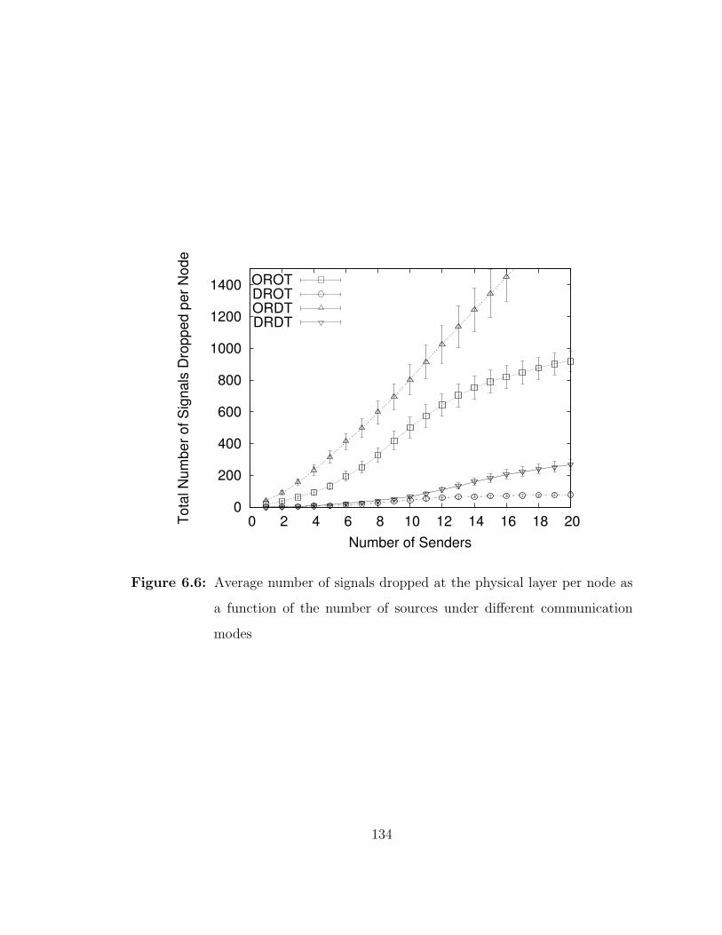
0
200
400
600
800
1000
1200
1400
0 2 4 6 8 10 12 14 16 18 20Tota
l Num
ber o
f Sig
nals
Dro
pped
per
Nod
e
Number of Senders
OROTDROTORDTDRDT
Figure 6.6: Average number of signals dropped at the physical layer per node as
a function of the number of sources under different communication
modes
134
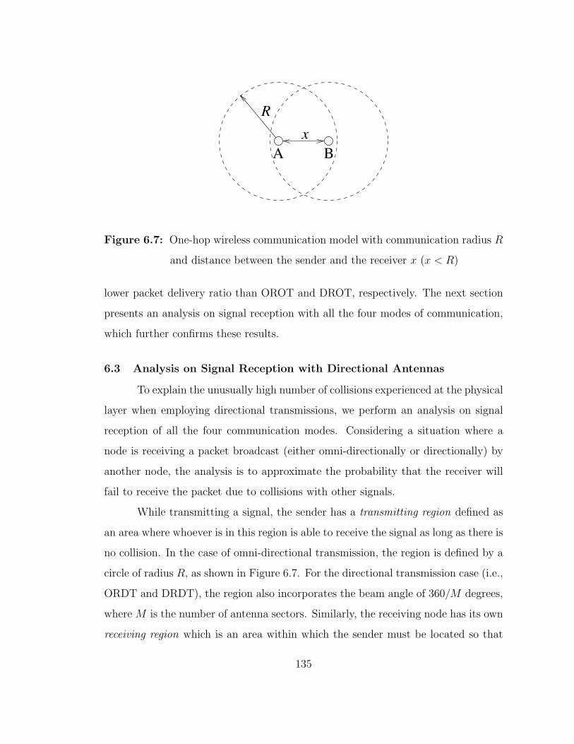
x
R
A B
Figure 6.7: One-hop wireless communication model with communication radius R
and distance between the sender and the receiver x (x < R)
lower packet delivery ratio than OROT and DROT, respectively. The next section
presents an analysis on signal reception with all the four modes of communication,
which further confirms these results.
6.3 Analysis on Signal Reception with Directional Antennas
To explain the unusually high number of collisions experienced at the physical
layer when employing directional transmissions, we perform an analysis on signal
reception of all the four communication modes. Considering a situation where a
node is receiving a packet broadcast (either omni-directionally or directionally) by
another node, the analysis is to approximate the probability that the receiver will
fail to receive the packet due to collisions with other signals.
While transmitting a signal, the sender has a transmitting region defined as
an area where whoever is in this region is able to receive the signal as long as there is
no collision. In the case of omni-directional transmission, the region is defined by a
circle of radius R, as shown in Figure 6.7. For the directional transmission case (i.e.,
ORDT and DRDT), the region also incorporates the beam angle of 360/M degrees,
where M is the number of antenna sectors. Similarly, the receiving node has its own
receiving region which is an area within which the sender must be located so that
135
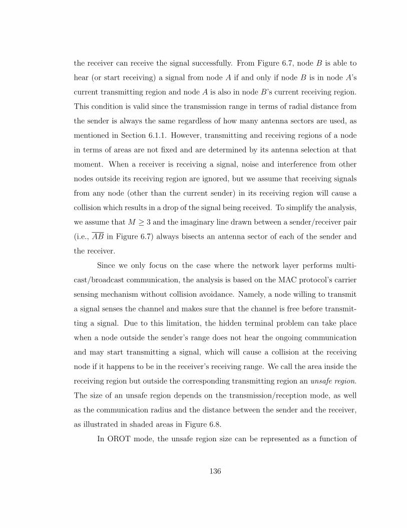
the receiver can receive the signal successfully. From Figure 6.7, node B is able to
hear (or start receiving) a signal from node A if and only if node B is in node A’s
current transmitting region and node A is also in node B’s current receiving region.
This condition is valid since the transmission range in terms of radial distance from
the sender is always the same regardless of how many antenna sectors are used, as
mentioned in Section 6.1.1. However, transmitting and receiving regions of a node
in terms of areas are not fixed and are determined by its antenna selection at that
moment. When a receiver is receiving a signal, noise and interference from other
nodes outside its receiving region are ignored, but we assume that receiving signals
from any node (other than the current sender) in its receiving region will cause a
collision which results in a drop of the signal being received. To simplify the analysis,
we assume that M ≥ 3 and the imaginary line drawn between a sender/receiver pair
(i.e., AB in Figure 6.7) always bisects an antenna sector of each of the sender and
the receiver.
Since we only focus on the case where the network layer performs multi-
cast/broadcast communication, the analysis is based on the MAC protocol’s carrier
sensing mechanism without collision avoidance. Namely, a node willing to transmit
a signal senses the channel and makes sure that the channel is free before transmit-
ting a signal. Due to this limitation, the hidden terminal problem can take place
when a node outside the sender’s range does not hear the ongoing communication
and may start transmitting a signal, which will cause a collision at the receiving
node if it happens to be in the receiver’s receiving range. We call the area inside the
receiving region but outside the corresponding transmitting region an unsafe region.
The size of an unsafe region depends on the transmission/reception mode, as well
as the communication radius and the distance between the sender and the receiver,
as illustrated in shaded areas in Figure 6.8.
In OROT mode, the unsafe region size can be represented as a function of
136
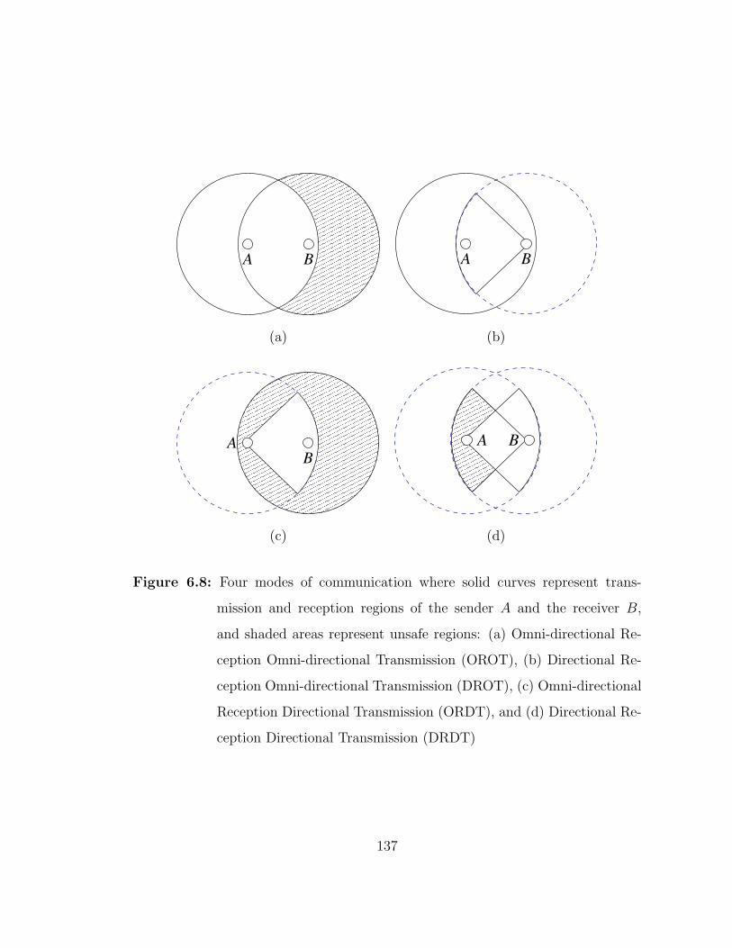
������������������������������������������������������������������������������������������������������������������������������������������������������������������������������������������������������������������������������������������������������������������������������������������������������������������
������������������������������������������������������������������������������������������������������������������������������������������������������������������������������������������������������������������������������������������������������������������������������������������������������������������
A B A B
(a) (b)
������������������������������������������������������������������������������������������������������������������������������������������������������������������������������������������������������������������������������������������������������������������������������������������������������������������
������������������������������������������������������������������������������������������������������������������������������������������������������������������������������������������������������������������������������������������������������������������������������������������������������������������
BA
���������������������������������������������������������������������������������������������������������������������
���������������������������������������������������������������������������������������������������������������������
A B
(c) (d)
Figure 6.8: Four modes of communication where solid curves represent trans-
mission and reception regions of the sender A and the receiver B,
and shaded areas represent unsafe regions: (a) Omni-directional Re-
ception Omni-directional Transmission (OROT), (b) Directional Re-
ception Omni-directional Transmission (DROT), (c) Omni-directional
Reception Directional Transmission (ORDT), and (d) Directional Re-
ception Directional Transmission (DRDT)
137

the distance between the sender and the receiver, x, and the communication radius,
R.
uorot(x, R) = πR2 − 2(R2 arccos
x
2R− x
4
√4R2 − x2
), (6.1)
where 0 < x < R.
For the other modes where directional antennas are employed either for trans-
mission or reception, or both, their unsafe regions also depend on the number of
antenna sectors, M . However, according to the analytical model, DROT does not
exhibit an unsafe region as long as each directional antenna consists of at least three
sectors (M ≥ 3). Therefore,
udrot(x, R,M) = 0. (6.2)
For ORDT, the size of its unsafe region is an area of a circle of radius R,
subtracted by an area covered by a single antenna sector, as follows:
uordt(x, R,M) =M − 1
MπR2. (6.3)
Finally, the unsafe region of DRDT can be formulated as:
udrdt(x, R,M) =πR2
M− x2
2tan
π
M. (6.4)
An average size of the unsafe region exhibited by each communication mode
for any sender/receiver pair can be computed by integrating each of (6.1), (6.2),
(6.3), and (6.4), weighted by the probability density function of the distance between
the two nodes. Let X be a random variable representing the distance between a
pair of sender and receiver. We have:
Prob{X < x} =πx2
πR2=
x2
R2.
Then the probability density function of X is:
pdf X(x) =d
dxProb{X < x} =
2x
R2.
138

Table 6.2: Sizes of unsafe regions exhibited by OROT, DROT, ORDT, and DRDT
with different numbers of antenna sectors, normalized to fractions of an
area covered by an omni-directional transmission
# antenna sectorsCommunication mode
M = 4 M = 6 M = 8
OROT 0.414 0.414 0.414
DROT 0.000 0.000 0.000
ORDT 0.750 0.833 0.875
DRDT 0.170 0.121 0.092
Now we can calculate the average unsafe region’s sizes for the four communication
modes as follows:
Uorot(R) =
∫ R
0
uorot(x, R)
(2x
R2
)dx = 3R2
(√3
4
). (6.5)
Udrot(R,M) =
∫ R
0
udrot(x, R,M)
(2x
R2
)dx = 0. (6.6)
Uordt(R,M) =
∫ R
0
uordt(x, R,M)
(2x
R2
)dx = πR2
(M − 1
M
). (6.7)
Udrdt(R,M) =
∫ R
0
udrdt(x, R,M)
(2x
R2
)dx = R2
(π
M− 1
4tan
π
M
). (6.8)
Table 6.2 shows average sizes of unsafe regions for different communication
modes with different number of antenna sectors as fractions of an area covered by
an omni-directional transmission (i.e., an area of a circle with radius R, or πR2). It
can be observed that DROT gives the smallest unsafe region, while ORDT yields
139
the largest. ORDT’s unsafe region grows larger as the number of antenna sectors
increases. On the other hand, DRDT’s unsafe region becomes smaller with higher
numbers of sectors.
To illustrate how these unsafe regions impact signal reception at a receiver,
we calculate the probability that a signal is dropped due to a collision. Considering
a wireless network of N nodes uniformly distributed over a terrain of size T , the
following traffic condition is assumed. Every node generates a packet to be sent
to one or more of its one-hop neighbors chosen randomly at a constant rate of r
packets per second. All packets are of a constant length, each of which requires a
transmission time τ seconds. The transmissions are not synchronized and τ is very
small in comparison to 1/r. Since a certain type of packets, such as HELLO’s, are
supposed to be received by all neighbors, we define pomni to represent the fraction
of these packets which are required to be transmitted omni-directionally, regardless
of the communication mode.
Given the number of nodes in the network and the terrain size, as well as the
size of the unsafe region U which is the corresponding function among (6.5), (6.6),
(6.7), and (6.8), the number of nodes in the unsafe region, with respect to a certain
receiver, is NUT
. In OROT and DROT, where packets are always transmitted omni-
directionally, a packet transmitted by any of these nodes will disrupt an ongoing
communication at the receiver. Therefore, the probability of a packet dropped due
to collision for OROT and DROT is equal to the probability that at least one of
nodes in the unsafe region will start transmitting a signal, which can be expressed
as:
Prob{collision|R}orot = 1− (1− rτ)NUorot (R)/T . (6.9)
Prob{collision|R,M}drot = 1− (1− rτ)NUdrot (R,M)/T = 0. (6.10)
The analysis is more complicated when directional transmissions are sup-
ported (i.e., ORDT and DRDT) because nodes do not always transmit packets
140
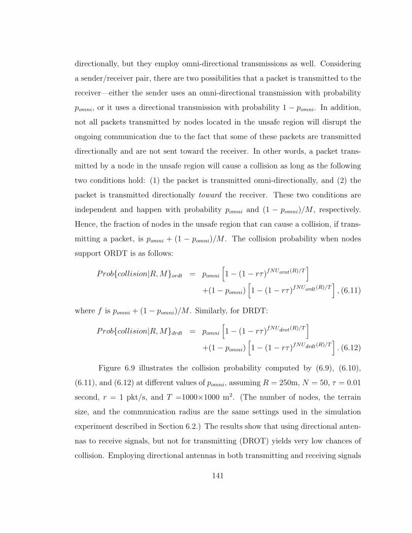
directionally, but they employ omni-directional transmissions as well. Considering
a sender/receiver pair, there are two possibilities that a packet is transmitted to the
receiver—either the sender uses an omni-directional transmission with probability
pomni, or it uses a directional transmission with probability 1 − pomni. In addition,
not all packets transmitted by nodes located in the unsafe region will disrupt the
ongoing communication due to the fact that some of these packets are transmitted
directionally and are not sent toward the receiver. In other words, a packet trans-
mitted by a node in the unsafe region will cause a collision as long as the following
two conditions hold: (1) the packet is transmitted omni-directionally, and (2) the
packet is transmitted directionally toward the receiver. These two conditions are
independent and happen with probability pomni and (1 − pomni)/M , respectively.
Hence, the fraction of nodes in the unsafe region that can cause a collision, if trans-
mitting a packet, is pomni + (1 − pomni)/M . The collision probability when nodes
support ORDT is as follows:
Prob{collision|R,M}ordt = pomni
[1− (1− rτ)fNUorot (R)/T
]+(1− pomni)
[1− (1− rτ)fNUordt (R)/T
], (6.11)
where f is pomni + (1− pomni)/M . Similarly, for DRDT:
Prob{collision|R,M}drdt = pomni
[1− (1− rτ)fNUdrot (R)/T
]+(1− pomni)
[1− (1− rτ)fNUdrdt (R)/T
]. (6.12)
Figure 6.9 illustrates the collision probability computed by (6.9), (6.10),
(6.11), and (6.12) at different values of pomni, assuming R = 250m, N = 50, τ = 0.01
second, r = 1 pkt/s, and T =1000×1000 m2. (The number of nodes, the terrain
size, and the communication radius are the same settings used in the simulation
experiment described in Section 6.2.) The results show that using directional anten-
nas to receive signals, but not for transmitting (DROT) yields very low chances of
collision. Employing directional antennas in both transmitting and receiving signals
141
0
0.01
0.02
0.03
0.04
0.05
0.06
0 0.2 0.4 0.6 0.8 1
Col
lisio
n P
roba
bilit
y
Omni-directional Broadcast Fraction
OROTDROT
ORDT,M=4ORDT,M=8DRDT,M=4DRDT,M=8
Figure 6.9: Analytical probability of signal collision as a function of omni-
directional broadcast fraction (pomni) due to the presence of unsafe
regions in different communication modes
142
(DRDT) results in low collision probabilities as well, but still higher than those of
DROT due to the presence of unsafe regions. In addition, the use of a narrower
beam in signal transmission is likely to cause less collisions than using wider beams.
However, in ORDT, where directional antennas are used only when transmitting
packets, the collision probabilities are considerably higher than those of DROT and
DRDT. Chances of collision are greater as more omni-directional broadcasts are
performed in the network. At certain values of omni-directional broadcast fractions,
ORDT even causes more collisions than OROT. These collision probabilities cause a
significant performance degradation in terms of packet delivery in unacknowledged
communication such as multicast, as we have seen from the simulation results in
the previous section. Note that, in the simulation experiment, not only is a signal
dropped by a collision as we assume in the analytical model, but also by low SINR
(Signal to Interference and Noise Ratio) due to noise and accumulated interference
from other nodes outside the unsafe region. Despite this fact, the analytical results
are consistent with the simulation results shown in Figure 6.6, where ORDT causes
more signal drops than OROT due to the fact that the multicast protocol used in
the experiment employs periodic HELLO messages for neighbor discovery.
6.4 Improving Delivery Success Rate
Due to the broadcast nature of wireless communication in ad hoc networks,
multicast data can be received by multiple destinations in one transmission. There-
fore, forwarding a multicast packet with the broadcast mode at the MAC layer is
generally preferable to using multiple unicast transmissions. However, this has the
major drawback that the data forwarding is not guaranteed, especially associated
with the hidden terminal problem from unsafe regions described in the previous sec-
tion. We propose an acknowledgment-based enhancement as an attempt to reduce
the effect of collisions and increase packet delivery ratio. Our enhancement works
on a per-hop basis as follows. Each multicast data packet is tagged with the source
143
ID (the unique identification of the node who originated the packet) and a sequence
number. A multicast protocol exploiting this enhancement is required to have a
mechanism that allows each forwarder or member (i.e., nodes that are currently
part of the multicast tree or mesh) to maintain a list of all the next-hop forwarders
and members of the same group. When a source or a forwarder has a data packet
to send, it broadcasts the packet normally and starts a retransmission timer. Upon
receiving this packet, each of the neighboring forwarders or members acknowledges
by transmitting an ACK packet back to the sender. To reduce the likelihood of
simultaneous transmissions that cause collisions of ACK packets at the sender node,
each receiver waits for a small random time before sending back an ACK packet.
When the sender’s timer expires and not all the expected ACKs have been received,
the sender rebroadcasts the same multicast packet. In addition, if ORDT or DRDT
mode is used, the packet will be rebroadcast only to the directions on which the
unacknowledged receivers are located, as illustrated in Figure 6.10. The sender gives
up after a certain number of rebroadcasts.
Using this means, packet forwarding has higher chances of success without
always sending the same multicast data packet repeatedly to multiple recipients
through unicast transmissions, which is expensive since the size of data packets is
much larger compared to ACK packets. This, however, comes with the price of
putting more control overhead on the channel. Despite the reduction of the overall
throughput of the network due to the use of extra ACK packets, the simulation
results in Section 6.5 show that, by incorporating this acknowledgment feature with
DRDT mode, nearly 100% packet delivery (> 99.7%) can be obtained when the
traffic load is not too high. Note that this enhancement only aims to increase
packet delivery ratio. It does not guarantee 100% delivery and is not intended to
provide an overall reliable multicast service.
144
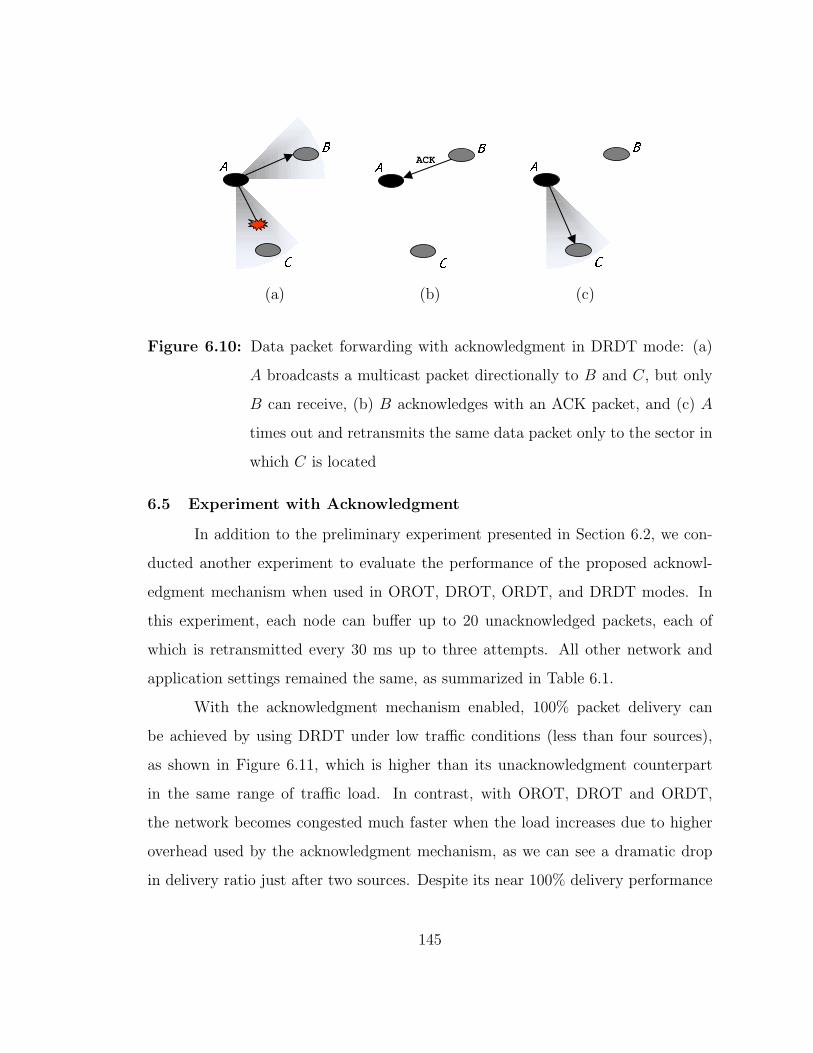
�
�
�
�
�
�
ACK
�
�
�
(a) (b) (c)
Figure 6.10: Data packet forwarding with acknowledgment in DRDT mode: (a)
A broadcasts a multicast packet directionally to B and C, but only
B can receive, (b) B acknowledges with an ACK packet, and (c) A
times out and retransmits the same data packet only to the sector in
which C is located
6.5 Experiment with Acknowledgment
In addition to the preliminary experiment presented in Section 6.2, we con-
ducted another experiment to evaluate the performance of the proposed acknowl-
edgment mechanism when used in OROT, DROT, ORDT, and DRDT modes. In
this experiment, each node can buffer up to 20 unacknowledged packets, each of
which is retransmitted every 30 ms up to three attempts. All other network and
application settings remained the same, as summarized in Table 6.1.
With the acknowledgment mechanism enabled, 100% packet delivery can
be achieved by using DRDT under low traffic conditions (less than four sources),
as shown in Figure 6.11, which is higher than its unacknowledgment counterpart
in the same range of traffic load. In contrast, with OROT, DROT and ORDT,
the network becomes congested much faster when the load increases due to higher
overhead used by the acknowledgment mechanism, as we can see a dramatic drop
in delivery ratio just after two sources. Despite its near 100% delivery performance
145
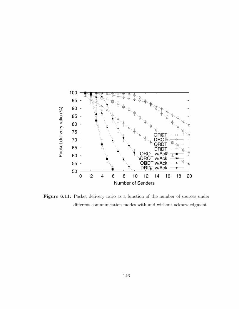
50
55
60
65
70
75
80
85
90
95
100
0 2 4 6 8 10 12 14 16 18 20
Pac
ket d
eliv
ery
ratio
(%)
Number of Senders
OROTDROTORDTDRDT
OROT w/AckDROT w/AckORDT w/AckDRDT w/Ack
Figure 6.11: Packet delivery ratio as a function of the number of sources under
different communication modes with and without acknowledgment
146
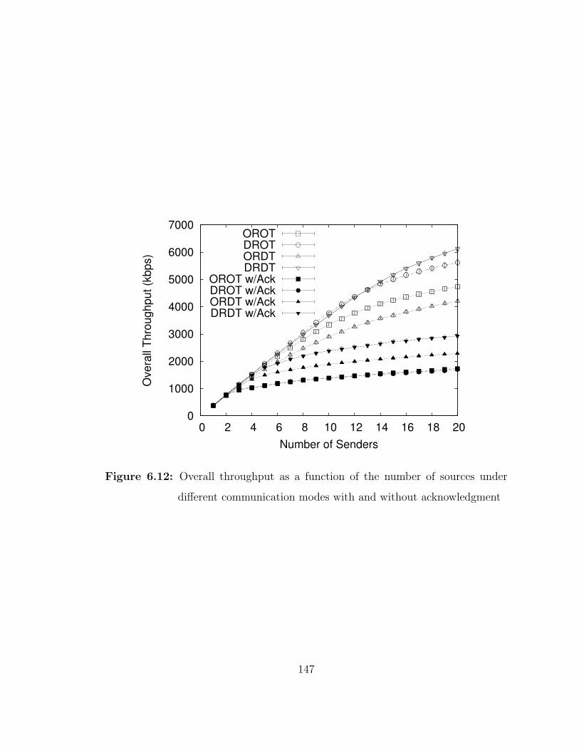
0
1000
2000
3000
4000
5000
6000
7000
0 2 4 6 8 10 12 14 16 18 20
Ove
rall
Thro
ughp
ut (k
bps)
Number of Senders
OROTDROTORDTDRDT
OROT w/AckDROT w/AckORDT w/AckDRDT w/Ack
Figure 6.12: Overall throughput as a function of the number of sources under
different communication modes with and without acknowledgment
147
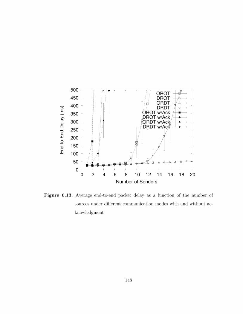
0
50
100
150
200
250
300
350
400
450
500
0 2 4 6 8 10 12 14 16 18 20
End
-to-E
nd D
elay
(ms)
Number of Senders
OROTDROTORDTDRDT
OROT w/AckDROT w/AckORDT w/AckDRDT w/Ack
Figure 6.13: Average end-to-end packet delay as a function of the number of
sources under different communication modes with and without ac-
knowledgment
148

under low traffic load, DRDT with acknowledgment is not able to handle moderate
and high load very well, as packet delivery ratio drops sharply after four sources
and end-to-end delay gets very large (Figure 6.13). Figure 6.12 shows that OROT
and DROT with acknowledgment yield equal overall network capacity. ORDT and
DRDT with acknowledgment can handle approximately 35% and 70% more traffic,
respectively, than the other two modes before the network gets saturated. However,
the maximum throughputs obtained from ORDT and DRDT with acknowledgment
are still much less than those of the unacknowledged versions of all the four modes.
With over 98% delivery ratio for up to ten sources, DROT without acknowl-
edgment seems to be the best scheme when considering packet delivery, due to its
minimum presence of unsafe regions. In contrast, DRDT without acknowledgment
is advantageous when end-to-end delay becomes more important. Despite the use
of narrow beams to transmit signals, ORDT exhibits a relatively large unsafe re-
gion which is prone to collisions and makes it undesirable mode for unacknowledged
data transfers. We believe that the benefit of directional transmissions will be more
significant when ORDT and DRDT operate in conjunction with an appropriate ac-
knowledgment mechanism. Apparently, the proposed acknowledgment scheme yields
high overhead and does not handle moderate and high traffic load very well, which
may not be desirable in general.
6.6 Summary
We have studied the benefits and impacts of using directional antennas for
multicast communication in ad hoc networks. Multicast forwarding nodes can keep
track of the directions of their neighboring forwarders and group members, and pro-
vide direction information to the MAC protocol for efficient broadcast of multicast
packets. By conducting a performance comparison on four different communication
149
modes: OROT, DROT, ORDT, and DRDT, we found that using directional anten-
nas considerably improves the performance in most aspects over omni-directional
antennas, especially over dense networks with heavy traffic load. In addition, broad-
casting packets directionally can help reduce the average end-to-end packet delay
and increase the maximum overall throughput. However, using directional anten-
nas is not always beneficial, as we also found that directed broadcast of signals
(ORDT and DRDT modes) can degrade performance in terms of packet delivery
due to the presence of unsafe regions which increase the probability of packet loss in
unacknowledged communication. This problem becomes less significant for DRDT
under heavy load conditions, as packet loss due to buffer overflow dominates over
the loss from the channel interference. This implies that using directional anten-
nas for packet transmission can help increase the overall network capacity if used in
conjunction with packet reception. As an attempt to improve delivery ratio, we pro-
posed a simple per-hop acknowledgment mechanism which gives nearly 100% packet
delivery ratio when used in DRDT mode and the load is not too high. However,
the scheme may not be acceptable in general due to its poor performance under
moderate and high load. Our simulation results show that, in terms of packet deliv-
ery, DROT without acknowledgment gives the best overall performance for a wide
range of traffic load, while DRDT without acknowledgment is advantageous when
end-to-end delay is more important. Although our simulation was done on a specific
multicast protocol, this study should also apply to multicast protocols for ad hoc
networks in general.
150
Chapter 7
CONCLUSION
Multicast serves as a critical functionality for group communications that
allows one set of messages transmitted by a source to be delivered to multiple recip-
ients. Providing this functionality over mobile wireless ad hoc networks poses many
challenges due to their unique characteristics. While efficient multicast connectivity
is preferable when resources are scarce, multicast connectivity should also be robust
enough to cope with network dynamics caused by mobility and node/communication
failure. Our research focuses on developing techniques that balance between the
efficiency and the effectiveness of ad hoc multicast routing in various mobility con-
ditions. In addition, we also investigated the benefits and impacts of incorporating
directional antennas into ad hoc multicast routing protocols.
We conclude this dissertation by summarizing the contributions and future
research directions.
7.1 Summary of Accomplishments
• We developed a distributed clustering algorithm, termed Adaptive Dynamic
Backbone (ADB), which constructs and maintains a mobility-adaptive virtual
backbone infrastructure. We the designed the ADB-based Multicast (ADBM)
protocol which relies on the virtual backbone to provide a multicast routing
service in a wide range of mobility conditions. Simulation results showed
that ADBM performs efficiently and effectively under low mobility, yet still
151
effectively under extremely high mobility with various network and application
settings.
• We adapted the biological metaphor of swarm intelligence to design a novel
multicast routing protocol called MANSI (Multicast for Ad hoc Network with
Swarm Intelligence). By using small control packets that behave like biologi-
cal ants, MANSI resembles an adaptive distributed control system that allows
multicast connections of lower total costs to be learned (or discovered) over
time. MANSI also incorporates a mobility-adaptive mechanism that allows the
protocol to remain effective as mobility increases. Similar to ADBM, simula-
tion results have shown that MANSI performs both effectively and efficiently
in static or low-mobility environments, yet still effectively in highly dynamic
environments.
• We proposed the Evolutionary Multicast Routing Framework (EMRF) for ad
hoc networks. By dividing the reactive multicast routing process into two
phases: initialization and evolution, EMRF allows independent incorporation
of different mechanisms for the two phases. Using this framework, we can cre-
ate protocol instances that can quickly and efficiently establish initial multicast
connectivity and/or effectively improve the resulting connectivity via different
optimization techniques. To demonstrate EMRF, we presented a protocol that
integrates the virtual backbone construction mechanism provided by ADBM
and the swarm intelligence based optimization technique used in MANSI to
initialize and evolve multicast connectivity, respectively. The new protocol
is shown to yield similar performance as the MANSI protocol. This gives
us confidence that we may be able to initialize multicast meshes using any
existing virtual infrastructures, based on network conditions and operational
constraints, and have them evolve, by way of swarm intelligence for instance,
into similar and efficient states.
152
• We studied the benefits and impacts of using directional antennas for multicast
communication in ad hoc networks, both analytically and experimentally. Four
different modes of operations, Omnidirectional-Reception/Omnidirectional-
Transmission (OROT), Directional-Reception/Omnidirectional-Transmission
(DROT), Omnidirectional-Reception/Directional-Transmission (ORDT), and
Directional-Reception/Directional-Transmission (DRDT), were evaluated and
compared. By allowing the network, MAC and physical layers to exchange in-
formation on neighboring multicast forwarders/members and their directions,
signals can be broadcast to these nodes using narrower beams. The simulation
results show that transmitting signals directionally (by operating in DRDT
mode) helps reduce the average end-to-end packet delay and increase the net-
work capacity. However, DRDT is still outperformed by DROT in terms of
packet delivery ratio due to a greater effect of the hidden terminal problem.
We therefore proposed a simple per-hop acknowledgment mechanism to reduce
the effect of hidden terminal and increase packet delivery ratio.
7.2 Future Work
• Although ADB was originally designed to facilitate multicast routing, it can
be applied to other applications where clustering of nodes is required. For in-
stance, ADB was used in cluster-based ad hoc network management [SJSH02,
SSJ02, SSJ03], where cluster heads serve as manager nodes to collect manage-
ment information (e.g., partial network topology) from their cluster members.
Smaller clusters are formed by ADB in dynamic areas, which reflects the fact
that local topology information is changing frequently and should not be col-
lected in a high amount as it will be outdated soon. In contrast, larger clusters
in relatively static areas allow more information to be collected, as this infor-
mation rarely changes. In addition, ADB has been used in our research on
cluster-based topology control [SSL+04].
153
• MANSI can be extended to different variations of the multicast routing prob-
lem in wireless ad hoc networks, such as load balancing and power-aware rout-
ing, as listed in Table 4.1. For instance, if nodes are assigned different transmis-
sion powers with topology control techniques [HS03, HSSJ02b, SHJ, SSL+04],
MANSI will attempt to reduce the total power of the multicast connectivity
when each node’s cost is proportional to its transmission power.
• Although Chapter 5 illustrated only one instance of EMRF, other combina-
tions of techniques will also be investigated. In addition, since unicast is
considered an instance of multicast, we believe that this framework can be
generalized to support both unicast and multicast routing.
• From our study on applying directional antennas to multicast communica-
tions, we learned that transmitting signals directionally could give many ben-
efits in terms of end-to-end delay and network capacity. However, performing
multicast by employing the broadcast mode of certain MAC protocols (e.g.,
IEEE 802.11) has a drawback in terms of packet delivery ratio due to lack of
collision avoidance and/or acknowledgment. To maximize the benefit of direc-
tional antennas for multicast, better reliable broadcast schemes, preferably a
MAC-layer approach, should be investigated to improve packet delivery ratio.
• We will also explore the applicability of clustering and swarm intelligence based
optimization techniques in our research on sensor networking [JSS00, JSS01,
SSJ01, SJS00] to design more efficient and effective protocols.
154
BIBLIOGRAPHY
[Bas99] Stefano Basagni. Distributed Clustering for Ad hoc Networks. In IEEEInternational Symposium on Parallel Architectures, Algorithms, andNetworks (I-SPAN), pages 310–315, Perth, Western Australia, June1999.
[BDT99] Eric Bonabeau, Marco Dorigo, and Guy Theraulaz. Swarm intelli-gence: from natural to artificial systems. Oxford University Press,1999.
[BFC93] Tony Ballardie, Paul Francis, and Jon Crowcroft. Core-based trees(CBT): An Architecture for Scalable Inter-Domain Multicast Rout-ing. In Communications, architectures, protocols, and applications,San Francisco, CA, USA, September 13–17 1993.
[BGLA03] L. Bao and J.J. Garcia-Luna-Aceves. Topology Management in AdHoc Networks. Annapolis, MD, June 1–3 2003.
[BKJ83] Kadaba Barath-Kumar and Jeffrey M. Jaffe. Routing to MultipleDestinations in Computer Networks. IEEE Transactions on Commu-nications, 31(3), 1983.
[BLSG00] S. Bae, S. Lee, W. Su, and M. Gerla. The Design, Implementation,and Performance Evaluation of the On-Demand Multicast RoutingProtocol in Multihop Wireless Networks. IEEE Network, Special Issueon Multicasting Empowering the Next Generation Internet, 14(1):70–77, January/February 2000.
[BTD01] Stefano Basagni, Damla Turgut, and Sajal K. Das. Mobility-AdaptiveProtocols for Managing Large Ad Hoc Networks. In IEEE Interna-tional Conference on Communications (ICC), Helsinki, Finland, June2001.
[CD97] Gianni Di Caro and Marco Dorigo. AntNet: A Mobile Agents Ap-proach to Adaptive Routing. Technical Report IRIDIA/97-12, Uni-versite Libre de Bruxelles, Belgium, 1997.
155
[CD98] Gianni Di Caro and Marco Dorigo. Two Ant Colony algorithms forBest-Effort Routing Datagram Networks. In the Tenth IASTED Inter-national Conference on Parallel and Distributed Computing and Sys-tems (PDCS’98), Las Vegas, Nevada, October 28–31 1998.
[CGHG02] Chao-Hsien Chu, JunHua Gu, Xiang Dan Hou, and Qijun Gu. AHeuristic Ant Algorithm for Solving QoS Multicast Routing Prob-lem. In 2002 Congress on Evolutionary Computation CEC2002, pages1630–1635, 2002.
[CGZ98a] C. Chiang, M. Gerla, and L. Zhang. Adaptive Shared Tree Multicastin Mobile Wireless Networks. In GLOBECOM ’98, pages 1817–1822,November 1998.
[CGZ98b] C. Chiang, M. Gerla, and L. Zhang. Forwarding Group MulticastProtocol (FGMP) for Multihop, Mobile Wireless Networks. BaltzerCluster Computing, 1(2):187–196, 1998.
[CL00a] Daniel Camara and Antonio A.F. Loureiro. A GPS/Ant-Like RoutingAlgorithm for Ad hoc Networks. In IEEE Wireless Communicationsand Networking Conference (WCNC 2000), Chicago, IL, September2000.
[CL00b] Daniel Camara and Antonio A.F. Loureiro. A Novel Routing Algo-rithm for Ad hoc Networks. In 33rd Hawaii International Conferenceon System Sciences, Maui, Hawaii, January 4–7 2000.
[DC90] S.E. Deering and D.R. Cheriton. Multicast Routing in Datagram In-ternetworks and Extended LANs. ACM Transactions on ComputerSystems, 8(2):85–110, May 1990.
[DCG99] Marco Dorigo, Gianni Di Caro, and Luca M. Gambardella. Ant Al-gorithms for Discrete Optimization. Technical Report IRIDIA/98-10,Universite Libre de Bruxelles, 1999.
[DEF+96] S. Deering, D.L. Estrin, D. Farinacci, V. Jacobson, C.-G. Liu, andL. Wei. The PIM Architecture for Wide-Area Multicast Routing.IEEE/ACM Transactions on Networking, 4(2):153–162, April 1996.
[DGHV02] S. Das, S. V. Gosavi, W. H. Hsu, and S. A. Vaze. An Ant ColonyApproach for the Steiner Tree Problem. In Genetic and EvolutionaryComputing Conference, New York City, New York, 2002.
[Dij74] Edsger W. Dijkstra. Self-stabilizing systems in spite of distributed con-trol. Communications of the ACM, 17(11):643–644, November 1974.
156
[DMC96] Marco Dorigo, Vittorio Maniezzo, and Alberto Colorni. The Ant Sys-tem: Optimization by a colony of cooperating agents. IEEE Transac-tions on Systems, Man, and Cybernetics-Part B, 26(1):1–13, February1996.
[DMM02] Subir Kumar Das, B. S. Manoj, and C. Siva Ram Murthy. A DynamicCore Based Multicast Routing Protocol for Ad hoc Wireless Networks.In The ACM Symposium on Mobile Adhoc Networking and Computing(MobiHoc), Lausanne, Switzerland, June 9–11 2002.
[DS01] Vijay Devarapalli and Deepinder Sidhu. MZR: A Multicast Protocolfor Mobile Ad Hoc Networks. In IEEE International Conference onCommunications (ICC), Helsinki, Finland, June 2001.
[Eri94] Hans Eriksson. MBONE: The Multicast Backbone. Communicationsof the ACM, 37(8):54–60, 1994.
[GBS00] Sandeep K. S. Gupta, Abdelmadjid Bouabdallah, and Pradip K. Sri-mani. Self-Stabilizing Protocol for Shortest Path Tree for Multi-castRouting in Mobile Networks. In European Conference on ParallelProcessing, pages 600–604, 2000.
[GdWFM02] Michael Gerharz, Christian de Waal, Matthias Frank, and Peter Mar-tini. Link Stability in Mobile Wireless Ad Hoc Networks. In Pro-ceedings of the IEEE Conference on Local Computer Networks (LCN)2002, November 2002.
[GLAM99] J. Garcia-Luna-Aceves and E. Madruga. The Core-Assisted MeshProtocol. IEEE Journal on Selected Areas in Communications, 17(8),August 1999.
[GS99a] S. K. S. Gupta and P. K. Srimani. Using self-stabilization to designadaptive multicast protocol for mobile ad hoc networks. In DIMACSWorkshop on Mobile Networks and Computing, Rutgers University,NJ, March 1999.
[GS99b] Sandeep K. S. Gupta and Pradip K. Srimani. An Adaptive Protocol forReliable Multicast in Multi-hop Radio Networks. In 2nd IEEE Work-shop on Mobile Computing Systems and Applications (WMCSA’99),pages 111–122, New Orleans, LA, February 1999.
[GS02] Mesut Gunes and Otto Spaniol. Routing Algorithms for Mobile Multi-Hop Ad-Hoc Networks. In International Workshop on Next Genera-tion Network Technologies. European Comission Central Laboratory
157

for Parallel Processings - Bulgarian Academy of Sciences, October2002.
[GS03] Sandeep K. S. Gupta and Pradip K. Srimani. Self-stabilizing multicastprotocols for ad hoc networks. Journal of Parallel and DistributedComputing, 63(1):87–96, January 2003.
[GSB01] Mesut Gunes, Udo Sorges, and Imed Bouazizi. ARA – The Ant-Colony Based Routing Algorithm for MANETs. In International Con-ference on Parallel Processing Workshops (ICPPW’02), Vancouver,B.C., Canada, August 18–21 2001.
[HB03] M. Heissenbuttel and T. Braun. Ants-Based Routing in Large ScaleMobile Ad-Hoc Networks. In Kommunikation in verteilten Systemen(KiVS03), Leipzig, Germany, March 25–28 2003.
[HOTV99] C. Ho, K. Obraczka, G. Tsudik, and K. Viswanath. Flooding forReliable Multicast in Multihop Ad Hoc Networks. In The 3rd Intl.workshop on Discrete Algorithms and Methods for Mobile Computingand Communications (DIAL-M’99), August 1999.
[HP96] Martin Horneffer and Dieter Plassmann. Directed Antennas in theMobile Broadband System. In IEEE INFOCOM’96, pages 704–712,San Francisco, CA, March 24–28 1996.
[HP97] Z. J. Haas and M. R. Pearlman. The zone routing proto-col (ZRP) for ad hoc networks, 1997. IETF Internet Draft.http://www.ietf.org/internet-drafts/draft-ietf-manet-zone-zrp00.txt.
[HP99] Z. Haas and M. Pearlman. Determining the Optimal Conguration forthe Zone Routing Protocol. In IEEE JSAC, August 1999.
[HS02] Zhuochuan Huang and Chien-Chung Shen. A Comparison Study ofOmnidirectional and Directional MAC Protocols for Ad Hoc Networks.In IEEE GLOBECOM, Taipei, Taiwan, November 17–21 2002.
[HS03] Zhuochuan Huang and Chien-Chung Shen. Poster: Distributed Topol-ogy Control Mechanism for Mobile Ad Hoc Networks with Swarm In-telligence. In The ACM Symposium on Mobile Adhoc Networking andComputing (MobiHoc), Annapolis, MD, June 1–3 2003.
[HSSJ02a] Zhuochuan Huang, Chien-Chung Shen, Chavalit Srisathapornphat,and Chaiporn Jaikaeo. A MAC Protocol Based on Directional Antennaand Busy-tone for Ad Hoc Networks. In IEEE MILCOM, Anaheim,California, October 7–10 2002.
158
[HSSJ02b] Zhuochuan Huang, Chien-Chung Shen, Chavalit Srisathapornphat,and Chaiporn Jaikaeo. Topology Control for Ad hoc Networks withDirectional Antennas. In IEEE International Conference on Com-puter Communications and Networks (ICCCN 2002), Miami, Florida,October 14–16 2002.
[JC98] Lusheng Ji and M. Scott Corson. A Lightweight Adaptive MulticastAlgorithm. In IEEE GLOBECOM’98, volume 2, pages 1036–1042,Sydney, Australia, November 1998.
[JJ01] Jorjeta G. Jetcheva and David B. Johnson. Adaptive Demand-DrivenMulticast Routing in Multi-Hop Wireless Ad Hoc Networks. In The2001 ACM International Symposium on Mobile Ad Hoc Networking &Computing, pages 33–44, Long Beach, CA, October 2001.
[JM01] David B. Johnson and David A. Maltz. The Dynamic Source Rout-ing Protocol for Mobile Ad Hoc Networks. Internet Draft (draft-ietf-manet-dsr-06.txt), November 2001. Work in Progress.
[JS02] Chaiporn Jaikaeo and Chien-Chung Shen. Adaptive Backbone-basedMulticast for Ad hoc Networks. In IEEE International Conference onCommunications (ICC 2002), New York City, NY, April 2002.
[JS03] Chaiporn Jaikaeo and Chien-Chung Shen. Multicast Communicationin Ad hoc Networks with Directional Antennas. In IEEE Interna-tional Conference on Computer Communication and Networks (IC-CCN 2003), Dallas, Texas, October 20–22 2003.
[JSS00] Chaiporn Jaikaeo, Chavalit Srisathapornphat, and Chien-Chung Shen.Querying and Tasking in Sensor Networks. In SPIE’s 14th AnnualInternational Symposium on Aerospace/Defense Sensing, Simulation,and Control, Orlando, Florida, April 2000.
[JSS01] Chaiporn Jaikaeo, Chavalit Srisathapornphat, and Chien-Chung Shen.Diagnosis of Sensor Networks. In IEEE International Conference onCommunications (ICC 2001), Helsinki, Finland, June 11–15 2001.
[KESI+02] Ioannis N. Kassabalidis, Mohamed A. El-Sharkawi, Robert J. MarksII, Payman Arabshahi, and Andrew A. Gray. Adaptive-SDR: Adap-tive Swarm-based Distributed Routing. In IEEE WCCI 2002, IJCNN2002 Special Session: Intelligent Signal Processing for Wireless Com-munications, Honolulu, Hawaii, May 12–17 2002.
159
[KKRM01] Ulas C. Kozat, George Kondylis, Bo Ryu, and Mahesh K. Marina.Virtual Dynamic Backbone for Mobile Ad Hoc Networks. In IEEEInternational Conference on Communications (ICC), Helsinki, Fin-land, June 2001.
[KR00] James F. Kurose and Keith W. Ross. Computer Networking: A Top-Down Approach Featuring the Internet. Addison-Wesley, 2000.
[KSV00] Young-Bae Ko, Vinaychandra Shankarkumar, and Nitin H. Vaidya.Medium Access Control Protocols using Directional Antennas in AdHoc Networks. In IEEE INFOCOM 2000, pages 13–21, Tel-Aviv,Israel, March 26–30 2000.
[LC99] Chunhun Richard Lin and Shiang-Wei Chao. A Multicast RoutingProtocol for Multihop Wireless Networks. In IEEE Global Telecommu-nications Conference (GLOBECOM), pages 235–239, Rio de Janeiro,Brazil, December 1999.
[LcK00] H. Lim and c. Kim. Multicast Tree Construction and Flooding in Wire-less Ad Hoc Networks. In ACM International Workshop on Modeling,Analysis and Simulation of Wireless and Mobile Systems (MSWIM),2000.
[LK00] Seungjoon Lee and Chongkwon Kim. Neighbor Supporting Ad hocMulticast Routing Protocol. In ACM/IEEE Workshop on Mobile AdHoc Networking and Computing (MobiHoc), pages 37–44, Boston, MA,August 11 2000.
[LLZ00] Guoying Lu, Zemin Liu, and Zheng Zhou. Multicast Routing Based onAnt Algorithm for Delay-Bounded and Load Balancing Traffic. In 25thAnnual IEEE Conference on Local Computer Networks (LCN’00),Tampa, FL, November 8–10 2000.
[LSG00] Sung-Ju Lee, William Su, and Mario Gerla. On-Demand MulticastRouting Protocol (ODMRP) for Ad Hoc Networks, 2000. IETF Inter-net Draft. http://www.ietf.org/proceedings/00jul/I-D/manet-odmrp-02.txt.
[LSH+00] Sung-Ju Lee, William Su, Julian Hsu, Mario Gerla, and Rajive Bagro-dia. A Performance Comparison Study of Ad Hoc Wireless MulticastProtocols. In IEEE INFOCOM 2000, pages 565–574, March 26–302000.
160

[LTM99] Mingyan Liu, Rajesh R. Talpade, and Anthony McAuley. AMRoute:Adhoc Multicast Routing Protocol. Technical Report 99, The Institutefor Systems Research, University of Maryland, 1999.
[Moy94] J. Moy. Multicast Routing Extensions for OSPF. Communications ofthe ACM, 37(8):61–66, August 1994.
[MTS02] Shivanajay Marwaha, Chen Kong Tham, and Dipti Srinavasan. Mo-bile Agents based Routing Protocol for Mobile Ad hoc Networks.In IEEE Global Telecommunications Conference (GLOBECOM’02),Taipei, Taiwan, November 17–21 2002.
[MWV00] N. Malpani, J. L. Welch, and N. H. Vaidya. Leader Election Al-gorithms for Mobile Ad Hoc Networks. Proceedings of the 4th in-ternational workshop on Discrete algorithms and methods for mobilecomputing and communications, pages 96–103, August 2000.
[MZ99] A. Bruce McDonald and Taieb F. Znati. A Mobility-Based Frameworkfor Adaptive Clustering in Wireless Ad hoc Networks. IEEE Journalon Selected Areas in Communications, 17(8), August 1999.
[NMMH00] Asis Nasipuri, Jothsna Mandava, Hanumantha Manchala, andRobert E. Hiromoto. On-Demand Routing Using Directional Anten-nas in Mobile Ad Hoc Networks. In IEEE International Conference onComputer Communication and Networks (ICCCN 2000), Las Vegas,October 2000.
[NYH00] Asis Nasipuri, Shengchun Ye, and Robert E. Hiromoto. A MAC Pro-tocol for Mobile Ad Hoc Networks Using Directional Antennas. InIEEE Wireless Communications and Networking Conference (WCNC2000), Chicago, September 2000.
[OKS99] Tomochika Ozaki, Jaime Bae Kim, and Tatsuya Suda. Bandwidth-Efficient Multicast Routing Protocol for Ad hoc Networks. In IEEEInternational Conference on Computer Communication and Networks(ICCCN’99), pages 10–17, Boston, MA, October 1999.
[OKS01] Tomochika Ozaki, Jaime Bae Kim, and Tatsuya Suda. Bandwidth-Efficient Multicast Routing for Multihop, Ad hoc Wireless Networks.In IEEE INFOCOM 2001, volume 2, pages 1182–1191, Anchorage,Alaska, April 22–26 2001.
[PC01] V. Park and S. Corson. Temporally-Ordered Routing Algorithm(TORA) (Internet-Draft), July 2001.
161
[PRD01] Charles E. Perkins, Elizabeth M. Royer, and Samir R. Das. Ad hoc On-Demand Distance Vector (AODV) Routing (Internet-Draft), March2001.
[RP99] R. Royer and C. Perkins. Multicast using ad-hoc on demand distancevector routing. In Mobicom’99, pages 207–218, Seattle, WA, August1999.
[Sca] Scalable Network Technologies, Inc. QualNet Simulator.
[SDB98] Raghupathy Sivakumar, Bevan Das, and Vaduvur Bharghavan. SpineRouting in Ad hoc Networks. ACM/Baltzer Publications Cluster Com-puting Journal, Special Issue on Mobile Computing, 1998.
[SGZ01] Marvin Sanchez, Tim Giles, and Jens Zander. CSMA/CA with BeamForming Antennas in Multihop Packet Radio. In Swedish workshopon Wireless Ad hoc Networks 2001, Stockholm, Sweden, March 2001.
[SHBR96] Ruud Schoonderwoerd, Owen Holland, Janet Bruten, and LeonRothkrantz. Ant-Based Load Balancing in Telecommunications Net-works. Technical Report HPL-96-76, Hewlett-Packart Laboraties Bris-tol, Bristol, UK, May 21 1996.
[SHJ] Chien-Chung Shen, Zhuochuan Huang, and Chaiporn Jaikaeo. Ant-Based Distributed Topology Control Algorithms for Mobile Ad HocNetworks. ACM Wireless Networks (WINET). accepted for publica-tion.
[SJ] Chien-Chung Shen and Chaiporn Jaikaeo. Ad hoc Multicast Rout-ing Algorithm with Swarm Intelligence. ACM Mobile Networks andApplications (MONET) Journal. accepted for publication.
[SJS00] Chavalit Srisathapornphat, Chaiporn Jaikaeo, and Chien-Chung Shen.Sensor Information Networking Architecture. In International Work-shop on Pervasive Computing (IWPC 2000), in conjunction withICPP 2000, Toronto, Canada, August 21–24 2000.
[SJSH02] Chien-Chung Shen, Chaiporn Jaikaeo, Chavalit Srisathapornphat, andZhuochuan Huang. The Guerrilla Management Architecture for Adhoc Networks. In IEEE MILCOM, Anaheim, California, October 7–10 2002.
[SSB99a] P. Sinha, R. Sivakumar, and V. Bharghavan. CEDAR: A Core-Extraction Distributed Ad hoc Routing Algorithm. In IEEE INFO-COM’99, New York City, NY, March 21–25 1999.
162
[SSB99b] Prasun Sinha, Raghupathy Sivakumar, and Vaduvur Bharghavan.MCEDAR: Multicast Core-Extraction Distributed Ad hoc Rout-ing. In IEEE Wireless Communications and Networking Conference(WCNC’99), pages 1313–1317, New Orleans, LA, September 1999.
[SSJ01] Chien-Chung Shen, Chavalit Srisathapornphat, and Chaiporn Jaikaeo.Sensor Information Networking Architecture and Applications. IEEEPersonel Communications Magazine, 8(4):52–59, August 2001.
[SSJ02] Chien-Chung Shen, Chavalit Srisathapornphat, and ChaipornJaikaeo. Adaptive Autonomous Management of Ad hoc Networks.In IEEE/IFIP Network Operations and Management Symposium(NOMS), Florence, Italy, April 15–19 2002.
[SSJ03] Chien-Chung Shen, Chavalit Srisathapornphat, and Chaiporn Jaikaeo.An Adaptive Management Architecture for Ad hoc Networks. IEEECommunications, 41(2):108–115, February 2003.
[SSL+04] Chien-Chung Shen, Chavalit Srisathapornphat, Rui Liu, ZhuochuanHuang, Chaiporn Jaikaeo, and Errol L. Lloyd. CLTC: A Cluster-basedTopology Control Framework for Ad hoc Networks. IEEE Transac-tions on Mobile Computing, 3(1):18–32, January/February 2004.
[TGB00] C.-K. Toh, Guillermo Guichal, and Santithorn Bunchua. ABAM:On-Demand Associativity-Based Multicast Routing for Ad hoc Mo-bile Networks. In IEEE Vehicular Technology Conference, VTC 2000,pages 987–993, September 2000.
[WT99] C.W. Wu and Y.C. Tay. AMRIS: A Multicast Protocol for Ad hocWireless Networks. In IEEE Military Communications Conference(MILCOM), pages 25–29, Atlantic City, NJ, November 1999.
163