www.oeaw.ac.at

www.ricam.oeaw.ac.at

Adaptive multi-parameterregularization in

electrochemical impedancespectroscopy

M. Žic, S. Pereverzyev Jr.

RICAM-Report 2018-16

1

Adaptive multi-parameter regularization in electrochemical impedance spectroscopy

Mark Žica,*+ and Sergiy Pereverzyev Jr.b*

a A JESH-guest researcher at Johann Radon Institute for Computational and Applied Mathematics (RICAM),

Altenbergerstrasse 69, A-4040 Linz, Austria b Universitätsklinik für Neuroradiologie, Medizinische Universität Innsbruck, Anichstrasse 35, A-6020 Innsbruck, Austria

Abstract

Determination of the distribution function of relaxation times (DFRT) is an approach to the

interpretation of Electrochemical Impedance Spectroscopy (EIS) measurements that maps these data into

a function containing the timescale characteristics of the system under consideration. The extraction of

such characteristics from noisy EIS measurements can be described by Fredholm interval equation of the

first kind, which is known to be ill-posed and can be treated only with regularization techniques.

Moreover, since only a finite number of EIS measurements may actually be performed, the above-

mentioned equation appears as after application of a collocation method that needs to be combined with

the regularization. Although in the regularization theory, such a combination has been studied and in

principle can alone be used for solving the problems, it is suggested in the EIS literature to employ

additional discretization of the corresponding Fredholm integral operator by quadrature or pseudo-

spectral (projection) methods that of course, might increase the approximation error.

In the present study, we discuss how a regularized collocation of DFRT problem can be implemented

such that all appearing quantities allow symbolic computations as sums of table integrals, and no

additional discretization steps are required.

In the proposed implementation of the regularized collocation it is treated as a multi-parameter

regularization, and another contribution of the present work is the adjustment of the previously proposed

multiple parameter choice strategy to the context of DFRT problem. The resulting strategy is based on

the aggregation of all computed regularized approximants, and can be in principle used in synergy with

other methods for solving DFRT problem. We also report the results from the synthetic experiments

showing that the proposed technique successfully reproduced known exact DFRT.

Keywords: EIS; DFRT; ill-posed problem; regularization; Python.

* Corresponding authors. E-mail addresses: mzic@irb.hr (M. Žic) and sergiy.pereverzyev@i-med.ac.at (S. Pereverzyev Jr.). + Present address: Ruđer Bošković Institute, P.O. Box 180, 10000 Zagreb, Croatia.

2

1. Introduction

In electrochemical impedance spectroscopy (EIS), the experiments are usually interpreted fitting

complex-valued impedance measurements 𝑍(𝜔𝑗) = 𝑍′(𝜔𝑗) + 𝑖𝑍′′(𝜔𝑗), 𝑗 = 0,1, … ,𝑁 − 1, against

chosen equivalent electrical circuit models. One of such models is known as the Voight circuit [1] and

composed of a series of parallel capacitors 𝐶𝑚 and resistors 𝑅𝑚, 𝑚 = 0,1, … ,𝑀 − 1, for which the

impedance writes:

𝑍(𝜔𝑗) = ∑𝑅𝑚

1 + 𝑖𝜔𝑗𝜏𝑚

𝑀−1

𝑚=0

, 𝑗 = 0,1, … ,𝑁 − 1, (1)

where 𝜏𝑚 = 𝑅𝑚𝐶𝑚. Note that sometimes an ohmic frequency independent part of the impedance is added

to (1), which can potentially be directly estimated from impedance measurements for large angular

frequencies and omitted here for simplicity.

Moreover, EIS experiments often cannot be described by a finite number of simple resistor-capacitor

(RC) elements, because they involve distributed time constants. Then a Voigt circuit with an infinite

number of RC elements can also be used to fit the impedance data (𝑍(𝜔)), but instead of discrete values

𝑅𝑚 = 𝜏𝑚𝐶𝑚−1 one should think the resistance variation 𝑅 = 𝑔(𝜏) with time 𝜏and deal with a continuous

version of (1) such as

𝑍(𝜔) = ∫𝑔(𝜏)𝑑𝜏

1 + 𝑖𝜔𝜏

∞

0

, (2)

where 𝑔(𝜏) describes the time relaxation characteristic of the electrochemical system under study.

Up to a certain extent 𝑔(𝜏) provides a circuit model-free representation of essential relaxation times that

are directly connected to the charge transfer process, because not only Voigt circuit, but also other known

circuit models, such as a constant phase element, Cole-Cole model, Davidson-Cole model, Warburg

element, etc., can be discussed in terms of the equation (2).

Since we are interested in a real-valued solution 𝑔(𝜏) of (2), this equation can be reformulated into

the system of equations with integral equations 𝐴1, 𝐴2:

{

(𝐴1𝑔)(𝜔) = ∫

𝑔(𝜏)𝑑𝜏

1 + 𝜔2𝜏2= 𝑍′(𝜔),

∞

0

(𝐴2𝑔)(𝜔) = ∫𝜔𝜏𝑔(𝜏)𝑑𝜏

1 + 𝜔2𝜏2= −𝑍′′(𝜔),

∞

0

(3)

where 𝑍′(𝜔), 𝑍′′(𝜔) are real and imaginary parts of 𝑍(𝜔).

3

Observe that if instead of the whole function 𝑍(𝜔) only the impedance measurements 𝑍(𝜔𝑗) =

𝑍′(𝜔𝑗) + 𝑖𝑍′′(𝜔𝑗), 𝑗 = 0,1, … ,𝑁 − 1, are available, then it reduces the system (3) to a collocation and

can be abstractly written as

𝑇𝑁𝐴1𝑔 = 𝑇𝑁𝑍′, 𝑇𝑁𝐴2𝑔 = −𝑇𝑁𝑍

′′, (4)

where TN is the so-called sampling operator assigning to each function F() a vector of its values at the

collocation points 𝜔𝑗, i.e., 𝑇𝑁𝐹 = (𝐹(𝜔0), 𝐹(𝜔1),… , 𝐹(𝜔𝑁−1).

Recall that the collocation is a special form of discretization that arises when we replace the original

problem, such as (3), by one in a finite dimensional space. In case of collocation this space is just the

Euclidean space 𝑅𝑁 of vectors 𝑢 = (𝑢0, 𝑢1, … , 𝑢𝑁−1), 𝑣 = (𝑣0, 𝑣1, … , 𝑣𝑁−1) equipped with a scalar

product

< 𝑢, 𝑣 >𝑅𝑁= ∑ 𝛾𝑗𝑢𝑗𝑣𝑗

𝑁−1

𝑗=0

and the corresponding norm ‖∙‖𝑅𝑁; here the weights 𝛾𝑗 , 𝑗 = 0,1, … . , N − 1, are some positive numbers.

Note that if operators 𝐴1, 𝐴2 are considered to be acting from the space 𝐿2(0,∞) of real-values square

summable functions on (0,∞) then the equations (4), due to their finite dimension, are always solvable

at least in the sense of least squares. Moreover, least square solutions of (4) can be reduced to the

corresponding systems of N linear algebraic equations, such that no additional discretization is required

and, as a result, no additional discretization error is introduced. Therefore, the impedance measurements

considered as collocation data already hint at a way to approximate the solution of (2).

At the same time, in the literature one mainly finds two other approaches for approximate solving of

(2). According to one of them, the integral operators 𝐴1, 𝐴2 in (4) are additionally discretized by means

of quadrature formulas. This approach has been studied in [2-4].

The second approach, advocated in [5, 6], discretizes the operators 𝐴1, 𝐴2 in (4) by means of

projection (pseudo-spectral) methods onto the subspaces of piecewise linear or radial basis functions.

In both above mentioned approaches the level of additional discretization, measuring by the number

of knots of a quadrature formula or by the number of basics function, should be properly tuned. Such

tuning is especially crucial in the case of noisy impedance measurements, when regularization techniques

need to be employed to avoid numerical instabilities in solving (4). Then, according to the Regularization

theory (see, e.g. [7]) the level of additional discretization of 𝐴1, 𝐴2 in (4) should be coordinated with the

amount of regularization.

4

This topic has not been touched in the above mentioned literature. At the same time, this issue does

not even appear if in (4) no additional discretization of the operators 𝐴1, 𝐴2 is introduced. Therefore, in

the present paper we study an approach avoiding any additional discretization of the operators in (4). It

is known (see, e.g. [2]) that the imaginary and real components 𝑍′′(𝜔𝑗), 𝑍′(𝜔𝑗) of the impedance have

different importance. Then it seems to be reasonable to treat the equations (4) with different amount of

regularization. At the same time, in the above mentioned literature, the equations (4) are involved into a

regularization scheme governed by only one regularization parameter that does not allow a desired

flexibility in exercising the regularization. Therefore, in the present study, we follow [8] and employ a

multi-parameter regularization. Moreover, we use the idea [8] of an aggregation of regularized solutions

corresponding to different values of multiple regularization parameters that allows an automatic

regularization in the form of a toolbox.

2. Theory

2.1 A multi-parameter regularization of the collocated impedance equations

In this section we analyze a methodology for joint regularization of the collocation equations (4) that

leads to a multi-parameter regularization. The joint regularization can be formulated as the minimization

of the objective functional

Φ(𝑔) : = 𝜆1‖𝑇𝑁𝐴1𝑔 − 𝑇𝑁𝑍′‖𝑅𝑁2 + 𝜆2‖𝑇𝑁𝐴2𝑔 + 𝑇𝑁𝑍

′′‖𝑅𝑁2 + ‖𝑔‖𝐿2(0,∞)

2 . (5)

Here the first two terms are the measures of data misfit weighed with the regularization

parameters 𝜆1, 𝜆2 ⊆ (0,∞). These misfits measures are combined in (5) with a regularization measure.

In the spirit of the Tikhonov-Philips regularization the latter one is chosen as the norm of the solution

space 𝐿2(0,∞) generated by the scalar product

⟨f, g⟩L2(0,∞) ≔ ∫ 𝑓(𝜏)𝑔(𝜏)𝑑𝜏, 𝑓, 𝑔 ⊆ 𝐿2(0,∞)∞

0

. (6)

It is known, for example, from [8] that the regularized approximated solution 𝑔𝜆1,𝜆2(𝜏) of (4) minimizing

(5) can be found from the operator equation

g + λ1(TNA1)∗TNA1g + λ2(TNA2)

∗TNA2g = λ1(TN𝐴1)∗𝑇𝑁𝑍

′ − 𝜆2(𝑇𝑁𝐴2)∗𝑇𝑁𝑍

′′, (7)

where (𝑇𝑁𝐴1)∗ and (𝑇𝑁𝐴2)

∗ are the adjoins of 𝑇𝑁𝐴1 and 𝑇𝑁𝐴2 respectably. They are defined by the

relations

⟨𝑢, 𝑇𝑁𝐴1𝑓⟩𝑅𝑁 = ⟨(𝑇𝑁𝐴1)∗𝑢, 𝑓⟩𝐿2(0,∞), ⟨𝑢, 𝑇𝑁𝐴2𝑓⟩𝑅𝑁 = ⟨(𝑇𝑁𝐴2)

∗𝑢, 𝑓⟩𝐿2(0,∞), (8)

5

that should be satisfied for any 𝑓 ⊆ 𝐿2(0,∞) and 𝑢 = (𝑢0, 𝑢1, … , 𝑢𝑁−1) ⊆ 𝑅𝑁. In view of definition of

⟨·,·⟩𝑅𝑁 , 𝑇𝑁 and (3) we have

⟨𝑢, 𝑇𝑁𝐴1𝑓⟩𝑅𝑁 = ∑ 𝛾𝑗𝑢𝑗 (∫𝑓(𝜏)𝑑𝜏

1 + 𝜔𝑗2𝜏2

∞

0

) = ∫ (∑𝛾𝑗𝑢𝑗

1 + 𝜔𝑗2𝜏2

𝑁−1

𝑗=0

)∞

0

𝑓(𝜏)𝑑𝜏 = ⟨∑1

1 +𝜔𝑗2𝜏2

𝛾𝑗𝑢𝑗, 𝑓⟩𝐿2(0,∞)

𝑁−1

𝑗=0

.

𝑁−1

𝑗=0

Now from (8) we can conclude that for any 𝑢 = (𝑢0, 𝑢1, … , 𝑢𝑁−1) ⊆ 𝑅𝑁

(𝑇𝑁𝐴1)∗𝑢 = ∑

1

1 + 𝜔𝑗2𝜏2

𝛾𝑗𝑢𝑗

𝑁−1

𝑗=0

. (9)

On the other hand, by definition of the adjoint operator (𝑇𝑁𝐴1)∗ it should be N-dimensional operator

from L2(0,∞) to 𝑅𝑁 and, as such, it should allow the representation

(𝑇𝑁𝐴1)∗(·) = ∑ 𝑙𝑖(𝜏)⟨𝑒

𝑗,·⟩𝑅𝑁

𝑁−1

𝑗=0

, (10)

where 𝑙𝑗 ⊆ 𝐿2(0,∞), 𝑒𝑗 ⊆ 𝑅𝑁. Comparing this with (9) we arrive at the formulas

𝑙𝑗(𝜏) =1

1 + 𝜔𝑗2𝜏2

, 𝑒𝑗 = (𝑒0𝑗, 𝑒1𝑗, … , 𝑒𝑁−1

𝑗) ⊆ 𝑅𝑁 , 𝑒𝑘

𝑗= 𝛿𝑘𝑗. (11)

where 𝛿𝑘𝑗 is the Kronecker delta, i.e. 𝛿𝑘𝑗 = 0 for 𝑘 ≠ 𝑗, and 𝛿𝑗𝑗 = 1.

By similar assignment, we can also obtain that

(𝑇𝑁𝐴2)∗(·) = ∑ 𝑙𝑗(𝜏)⟨𝑒

𝑗−𝑁,·⟩𝑅𝑁 .

2𝑁−1

𝑗=𝑁

(12)

where

𝑙𝑗(𝜏) =𝜔𝑗−𝑁𝜏

1 + 𝜔𝑗−𝑁2 𝜏2

, 𝑗 = 𝑁,𝑁 + 1,… ,2𝑁 − 1. (13)

Now form (10)-(13) one can easily see that the solution of (7) admits the representation

𝑔𝜆1,𝜆2(𝜏) = ∑ 𝑔𝑗1

1 + 𝜔𝑗2𝜏2

𝑁−1

𝑗=0

+ ∑ 𝑔𝑗𝜔𝑗−𝑁𝜏

1 + 𝜔𝑗−𝑁2 𝜏2

2𝑁−1

𝑗=𝑁

. (14)

The unknown coefficients 𝑔𝑖 = 0,1, … ,2𝑁 − 1, can be found from the following system of linear

algebraic equations

{

𝑔𝑘 + 𝜆1 ∑ 𝑎1,𝑘,𝑗𝑔𝑗

2𝑁−1

𝑗=0

= 𝜆1𝛾 𝑘𝑍′(𝜔𝑘), 𝑘 = 0,1… ,𝑁 − 1

𝑔𝑘 + 𝜆2 ∑ 𝑎2,𝑘,𝑗𝑔𝑗

2𝑁−1

𝑗=0

= −𝜆2𝛾 𝑘−𝑁𝑍′′(𝜔𝑘−𝑁), 𝑘 = 𝑁,𝑁 + 1,… ,2𝑁 − 1

(15)

6

Where 𝑎1,𝑘,𝑁+𝑘 =𝛾𝑘

2𝜔𝑘, 𝑘 = 0,1,… ,𝑁 − 1,

𝑎1,𝑘,𝑗 =

{

∫

𝛾𝑘𝑑𝜏

(1 + 𝜔𝑘2𝜏2)(1 + 𝜔𝑗

2𝜏2)

∞

0

=𝜋𝛾𝑘

2(𝜔𝑘 + 𝜔𝑗),

𝑗 = 0,1,2,… ,𝑁 − 1,

∫𝛾𝑘 𝜔𝑗−𝑁𝜏𝑑𝜏

(1 + 𝜔𝑘2𝜏2)(1 + 𝜔𝑗−𝑁

2 𝜏2)

∞

0

=𝛾𝑘𝜔𝑗−𝑁

(𝜔𝑘2 − 𝜔2𝑗−𝑁)

ln (𝜔𝑘𝜔𝑗−𝑁

) ,

𝑗 = 𝑁,… ,2𝑁 − 1; 𝑗 ≠ 𝑁 + 𝑘,

and 𝑎2,𝑘,𝑘−𝑁 =𝛾𝑘−𝑁

2𝜔𝑘−𝑁, 𝑘 = 𝑁,𝑁 + 1,… ,2𝑁 − 1,

𝑎2,𝑘,𝑗 =

{

∫

𝛾𝑘−𝑁 𝜔𝑘−𝑁𝜏𝑑𝜏

(1 + 𝜔𝑘−𝑁2 𝜏2)(1 + 𝜔𝑗

2𝜏2)

∞

0

=𝛾𝑘−𝑁𝜔𝑘−𝑁

(𝜔𝑘−𝑁2 − 𝜔𝑗

2)ln (

𝜔𝑘−𝑁𝜔𝑗

),

𝑗 = 0,1,2, … ,𝑁 − 1; 𝑗 ≠ 𝑘 − 𝑁,

∫𝜔𝑘−𝑁 𝜔𝑗−𝑁𝛾𝑘−𝑁 𝜏

2𝑑𝜏

(1 + 𝜔𝑘−𝑁2 𝜏2)(1 + 𝜔𝑗−𝑁

2 𝜏2)

∞

0

=𝜋

2𝛾𝑘−𝑁

1

𝜔𝑘−𝑁𝜔𝑗−𝑁 (𝜔𝑘−𝑁 + 𝜔𝑗−𝑁),

𝑗 = 𝑁,𝑁 + 1,… ,2𝑁 − 1.

From (14), (15) it is clear that for given 𝜆1, 𝜆2 the regularized approximate solution 𝑔𝜆1,𝜆2 of (4) can be

constructed without additional discretization of the integral operators 𝐴1, 𝐴2. In the next section we

discuss aggregation of 𝑔𝜆1,𝜆2 constructed for different values of the regularization parameters 𝜆1, 𝜆2.

2.2 Aggregation of 𝑔𝜆1,𝜆2in weighted norms

It is known that the solution 𝑔(𝜏) of the impedance equation (2) may have singularities at 𝜏 = 0. For

example, in a constant-phase element model [9] the solution 𝑔(𝜏) has the form

𝑔(𝜏) =1

2𝜋𝜏

sin [(1 − 𝜑)𝜋]

cosh [𝜑 ln (𝜏𝜏0)] − cos[(1 − 𝜑)𝜋]

, 𝜑 ⊆ (0,1),

and it is clear that 𝑔(𝜏) → ∞ with τ → 0.

In Mathematics (see, e.g., [10]) such solutions with singularities are usually studied in a space of

functions with a finite norm involving a functional multiplier-the weight 𝜌(𝜏). The norm of the function

𝜌(𝜏)𝑔(𝜏) is then called the weighed norm of 𝑔(𝜏). The introduction of a weight 𝜌(𝜏) makes it possible

to introduce into consideration the functions with infinite ordinary non-weighted norm. In most cases the

7

weight 𝜌(𝜏) tends to zero as its argument approaches the point of singularity 𝜏 = 0; so, the simplest

choice of the weights is 𝜌(𝜏) = 𝜏𝜈 , 𝜈 > 0

Note that in the literature on electrochemical impedance spectroscopy (EIS) the weighted solutions

𝜏𝜈𝑔(𝜏), 𝜈 = 1 of the impedance equation (2) are of interest by themselves (see, e.g. [2, 6]) and often

called as distribution functions of relaxation time (DFRT). Moreover, one is often interested in the

behavior DFRT only within a time window 𝜏 ⊆ [𝑊𝑚𝑖𝑛,𝑊𝑚𝑎𝑥] ⊂ [0,∞). Therefore, if �̃�(𝜏)is an

approximate solution of the impedance equation (2), such as �̃�(𝜏) = 𝑞𝜆1,𝜆2(𝜏), for example, then it seems

to be reasonable to measure approximation error in the weighted norm

‖𝑔 − �̃�‖𝐿2,𝜈(𝑊𝑚𝑖𝑛, 𝑊𝑚𝑎𝑥)= { ∫ [𝜏𝜈 𝑔(𝜏) − 𝜏𝜈�̃�(𝜏)]2𝑑𝜏

𝑊𝑚𝑎𝑥

𝑊𝑚𝑖𝑛

}

12

.

It is clear that this norm is a Hilbert space norm governed by the scalar product:

⟨𝑓, 𝑔⟩𝐿2,𝜈(𝑤𝑚𝑖𝑛,𝑊𝑚𝑎𝑥) = ∫ 𝜏2𝜈𝑔(𝜏)𝑓(𝜏)𝑑𝜏.𝑊𝑚𝑎𝑥

𝑊𝑚𝑖𝑛

While we have described the explicit procedure (14), (15) for approximating the solutions of (2)

directly from the impedance measurements, there is still a question about the choice of the regularization

parameters 𝜆1, 𝜆2 that determine suitable relative weighting between these measurements. By setting

𝜆1 = 0 or 𝜆2 = 0, one may reduce this question to the case discussed in [4]. In another particular case

𝜆1 = 𝜆2 = 𝜆, one may choose a suitable value of 𝛼 = 𝜆−1 by a cross-validation technique, as it was

suggested in [6]. In both particular cases, one in fact deals with a single-parameter regularization, where

many parameter choice strategies are available. A multi-parameter regularization is much less studied,

especially when multiple regularization parameters are employed to construct a common misfit measure

as in (5). In this direction one can only indicate the paper [8] and two references therein. Here we adjust

the idea of [8] to the contexts of EIS.

Note that known regularization parameter choice strategies usually consist in using some criteria for

selecting only one particular candidate from a family of approximate solutions calculated for different

values of regularization parameters from sufficiently wide range. In contrast, in [8] it is proposed to

construct a new approximate solution in the form of a linear combination of all calculated approximates.

In the present context this means, for example, that at first we calculate 𝑞𝜆1,𝜆2(𝜏) for some values 𝜆1 =

𝜆1,𝑝, 𝑝 = 0,1,2, … , 𝑃 − 1, 𝜆2 = 𝜆2,𝑞 , 𝑞 = 0,1,2, … , 𝑄 − 1, , deserving consideration, and then consider

a new approximate solution

8

�̃�(𝜏) = ∑ 𝑐𝑚𝑔𝑚(𝜏)

𝑃𝑄−1

𝑚=0

, (16)

where 𝑔𝑚(𝜏) = 𝑔𝜆1,𝑝,𝜆2,𝑞(𝜏), 𝑚 = 𝑃𝑞 + 𝑝, 𝑝 = 0,1,2, … , 𝑃 − 1, 𝑞 = 0,1,2, … , 𝑄 − 1,𝑚 =

0,1,2, … , 𝑃𝑄 − 1, and 𝑐𝑚 are coefficients to be determined.

In view of the discussion above, it is natural to choose the coefficients cm such that �̃� provides the

best approximation of the exact solution 𝑔 in the norm ‖∙‖𝐿2,𝜈(𝑊𝑚𝑖𝑛𝑊𝑚𝑎𝑥) among all linear combinations

(16). Since ‖∙‖𝐿2,𝜈(𝑊𝑚𝑖𝑛𝑊𝑚𝑎𝑥) is a Hilbert space norm, it is clear that the coefficient vector 𝑐 =

(𝑐0, 𝑐1, … , 𝑐𝑃𝑄−1) should solve the following matrix vector equation:

𝐺𝑐 ⃗⃗⃗ = �⃗�, (17)

where

�⃗� = (𝐹𝑚)𝑚=0𝑃𝑄−1, 𝐹𝑚 = ⟨𝑔, 𝑔𝑚⟩𝐿2,𝜈(𝑊𝑚𝑖𝑛,𝑊𝑚𝑎𝑥)

= ∫ 𝜏2𝜈𝑔(𝜏)𝑔𝑚(𝜏)𝑑𝜏𝑊𝑚𝑎𝑥

𝑊𝑚𝑖𝑛

,

𝐺 = (𝐺𝑚,𝑛)𝑚,𝑛=0𝑃𝑄−1

, 𝐺𝑚,𝑛 = ⟨𝑔𝑚, 𝑔𝑛⟩𝐿2,𝜈(𝑊𝑚𝑖𝑛, 𝑊𝑚𝑎𝑥)= ∫ 𝜏2𝜈𝑔𝑚(𝜏)𝑔𝑛(𝜏)𝑑𝜏.

𝑊𝑚𝑎𝑥

𝑊𝑚𝑖𝑛

If the regularized approximants

𝑔𝑚(𝜏) = 𝑔𝜆1,𝑝,𝜆2,𝑞(𝜏) = ∑ 𝑔𝑗𝑚𝑙𝑗(𝜏)

2𝑁−1

𝑗=0

, (18)

are already calculated from (14), (15), then the elements of the matrix 𝐺 can be exactly calculated as well. Indeed,

from (18) it follows that

𝐺𝑚,𝑛 = ∑ ∑ 𝑔𝑖𝑚

2𝑁−1

𝑖=0

𝑔𝑗𝑛𝑏𝑖,𝑗

2𝑁−1

𝑖=0

,

where

𝑏𝑖𝑗 = ⟨𝑙𝑖, 𝑙𝑗⟩𝐿2,𝜈(𝑊𝑚𝑖𝑛,𝑊𝑚𝑎𝑥)= ∫ 𝜏2𝜈𝑙𝑖(𝜏)𝑙𝑗(𝜏)𝑑𝜏

𝑊

𝑤

and 𝑙𝑖(𝜏), 𝑙𝑗(𝜏) are given by (11), (13). It is clear that the above integrals can be explicitly calculated. For example,

for 𝜈 = 1 and 𝑖, 𝑗 = 𝑁 + 1,… ,2𝑁 − 1 we have

9

𝑏𝑖𝑗 =

{

𝑊𝑚𝑎𝑥 −𝑊𝑚𝑖𝑛

𝜔𝑖−𝑁𝜔𝑗−𝑁+𝜔𝑗−𝑁3 tan−1(𝜔𝑖−𝑁𝜏) − 𝜔𝑖−𝑁

3 tan−1(𝜔𝑗−𝑁𝜏)

𝜔𝑖−𝑁2 𝜔𝑗−𝑁

2 (𝜔𝑖−𝑁2 −𝜔𝑗−𝑁

2 )|

𝜏=𝑊𝑚𝑖𝑛

𝜏=𝑊𝑚𝑎𝑥

, 𝑖 ≠ 𝑗

𝜔𝑖−𝑁𝜏 (2 + (1 + 𝜔𝑖−𝑁2 𝜏2)

−1) − 3 tan−1(𝜔𝑖−𝑁 𝜏)

2𝜔𝑖−𝑁3 |

𝜏=𝑊𝑚𝑖𝑛

𝜏=𝑊𝑚𝑎𝑥

, 𝑖 = 𝑗.

On the other hand, the components 𝐹𝑚 of the vector �⃗� in (17) depend on the unknown solution 𝑔 of (12),

and therefore are inaccessible.

At the same time, in [8] and [11] we can find an approach to estimate the components of the vector �⃗� by

using the so-called quasi-optimality criterion in the linear functional strategy. The advantage of this

approach is that the values of the scalar products 𝐹𝑚 = ⟨𝑔, 𝑔𝑚⟩𝐿2,𝜈(𝑊𝑚𝑖𝑛,𝑊𝑚𝑎𝑥)of the solution 𝑔 can be

estimated much more accurately than the solution 𝑔 in the norm ‖∙‖𝐿2,𝜈(𝑊𝑚𝑖𝑛𝑊𝑚𝑎𝑥).

According to [8, 11] we estimate the scalar product ⟨𝑔, 𝑔𝑚⟩ by ⟨𝑓𝛼 , 𝑔𝑚⟩𝐿2,𝜈(𝑊𝑚𝑖𝑛,𝑊𝑚𝑎𝑥)

, where 𝑓𝛼(𝜏) is the

regularized approximate solutions 𝑔𝜆1,𝜆2(𝜏) given by (14) and constructed for 𝜆1 = 0, 𝜆2 = 𝛼, with the use of

only imaginary part of the impedance data. The reasons for this is that , as known in the literature (see,

e.g. [2]) this part of data may allow better accuracy than the real part of the impedance.

In principle, the values of 𝜆2 = 𝛼 may be taken from the same set {𝜆2,𝑞}𝑞=0𝑄−1

as the one above. But in

[8, 11] it is suggested to take 𝛼 = 𝛼𝑠 from a geometric sequence 𝛼𝑠 = 𝛼0𝛽𝑠, 𝑠 = 0,1, … , 𝑆 − 1, 𝑆 > 𝑄.

Therefore, we consider

𝑓𝑠(𝜏) = ∑ 𝑔𝑗0,𝑠

2𝑁−1

𝑗−𝑁

𝑙𝑗(𝜏),

where 𝑔𝑗 = 𝑔𝑗0,𝑠

are the solutions of the linear system (15) with 𝜆1 = 0, 𝜆2 = 𝛼𝑠, 𝑠 = 0,1, … , 𝑆 − 1, and

⟨𝑓𝑠 , 𝑔𝑚⟩𝐿2,𝜏(𝑊𝑚𝑖𝑛,𝑊𝑚𝑎𝑥)

= ∑ ∑ 𝑔𝑖0,𝑠

2𝑁−1

𝑗=0

𝑔𝑗𝑚𝑏𝑖,𝑗

2𝑁−1

𝑖=𝑁

.

Then, according to the quasi-optimality criterion in the linear functional strategy [11] we select such 𝑠 =

𝑠𝑚 that

|⟨𝑓𝑠𝑚 , 𝑔𝑚⟩𝐿2,𝜈(𝑊𝑚𝑖𝑛,𝑊𝑚𝑎𝑥)

− ⟨𝑓𝑠𝑚−1, 𝑔𝑚⟩𝐿2,𝜈(𝑊𝑚𝑖𝑛,𝑊𝑚𝑎𝑥)

|

= 𝑚𝑖𝑛{|⟨𝑓𝑠, 𝑔𝑚⟩𝐿2,𝜈(𝑊𝑚𝑖𝑛,𝑊𝑚𝑎𝑥)

− ⟨𝑓𝑠−1, 𝑔𝑚⟩𝐿2,𝜈(𝑊𝑚𝑖𝑛,𝑊𝑚𝑎𝑥)

|, 𝑠 = 1,2, … , 𝑆 − 1}

The theoretical analysis of [11] quarantines that the values of 𝐹𝑚 = ⟨𝑔, 𝑔𝑚⟩ is well approximated by the

values of 𝐹�̃� = ⟨𝑓𝑠𝑚 , 𝑔𝑚⟩. Recall that vector 𝑐 of coefficients of the best linear combination of (16)

10

approximating the solution 𝑔 of (2) in the norm ‖∙‖𝐿2,𝜈(𝑊𝑚𝑖𝑛𝑊𝑚𝑎𝑥) should solve the matrix vector

equation (17).

According to aggregation strategy [8] we approximate this ideal vector by the vector �̃� = (�̃�0, �̃�1,…,�̃�𝑃𝑄−1)

solving in the least squares sense the approximate matrix vector equation

G�̃� = �̃�, �̃� = (�̃�0, �̃�1, … , �̃�𝑃𝑄−1). (19)

Then the theoretical analysis of [8] quarantines that the approximate solution

�̃�(𝜏) = ∑ �̃�𝑚𝑔𝑚(𝜏) =

𝑃𝑄−1

𝑚=0

∑ ∑ �̃�𝑚𝑔𝑗𝑚 1

1 + 𝜔𝑗2𝜏2

+

𝑁−1

𝑗=0

𝑃𝑄−1

𝑚=0

∑ ∑ �̃�𝑚𝑔𝑗𝑚

𝜔𝑗−𝑁𝜏

1 + 𝜔𝑗−𝑁2 𝜏2

2𝑁−1

𝑗=𝑁

𝑃𝑄−1

𝑚=0

, (20)

is almost as good as the best linear approximation (16) of the calculated regularized

solutions 𝑔𝜆1,𝑝,𝜆2,𝑞(𝜏).

Thus, we have described an adaptive procedure that automatically constructs an approximate solution of

(2) and theoretically should perform at the level of the best regularized approximant 𝑔𝜆1,𝜆2(𝜏) calculated

according to (14), (15) for a given range of 1,2. The input of the proposed procedure consists of the

impedance data 𝑍(𝜔𝑗), 𝑗 = 0,1, … ,𝑁 − 1, the weights 𝛾𝑗 , 𝑗 = 0,1, … , 𝑁 − 1 determining the misfits

measures, the endpoints 𝑊𝑚𝑖𝑛,𝑊𝑚𝑎𝑥 of the time window of interest, and the numbers 𝜆0,1, 𝜆0,2, 𝛼0, 𝑃, 𝑄, 𝑆

defining the range of the regularization parameters under consideration.

3. Results

In this section we test the performances of the approximations (14), (15) and (20). For this purpose,

we follow [5, 6] and employ analytically given impedance data 𝑍𝑒𝑥(𝜔) with known time relaxation

characteristics 𝑔(𝜏) that solve (2). These synthetic experiments are based on single and double ZARC

and Fractal element models [1]. To mimic the conditions of real EIS experiments, we add artificial noise

to an analytical impedance 𝑍𝑒𝑥(𝜔) and use one of the models form [4, 12] such that noisy data are

simulated as

𝑍(𝜔𝑗) = 𝑍𝑒𝑥(𝜔𝑗) + 휀𝑗′ + 𝑖휀𝑗

′′, 𝑗 = 0,1, … ,𝑁 − 1. (21)

where 휀𝑗′, 휀𝑗

′′ are independent normally distributed random variables with zero mean and variance 10-4;

the frequencies are sampled from the range 𝜔 ⊆ [10−2Hz, 106Hz] with 5 collocation points (𝜔𝑗) per

decade.

11

3.1 Software tools used in this work

The new Distribution of Relaxation Time (DFRT) strategy was developed by open source Python

2.7.15 programming language [13] which is widely used in the science community [14-17]. The

following essential Python open source modules were used in this work:

- Numpy [18] v1.14.3,

- Matplotlib [19] v2.2.2,

- wxPython v3.0.2.0,

- Cython 0.23.3 and

- PyInstaller v3.3.1.

The new DFRT approach was entirely coded from scratch and it relies heavily on NumPy module.

However, other presented modules were necessary for data presentation and to embed the new DFRT

strategy into the existing EisPy software package [20, 21].

3.2 Regularization (14), (15) with best tuned parameters

At first, we consider the situation, when in (14), (15) the regularization parameters 𝜆1, 𝜆2 are best-

tuned for one of the models, say single ZARC element, and then used for other ones too. We discuss such

an approach, because at first glance it may look as a reasonable parameter choice strategy, and at some

extent it works, but not always. As in [6], we consider the impedance response of a single ZARC element

model given by

𝑍𝑒𝑥(𝜔) = 𝑍𝑒𝑥,𝜙(𝜔, 𝜏0) =𝑅𝑐𝑡

1 + (𝑖𝜔𝜏0)𝜙,

(22)

where 𝑅𝑐𝑡 = 50 Ω, τ0 = 0.01 𝑠 and 𝜙 = 0.7. The corresponding solution 𝑔(𝜏) of (2) with 𝑍(𝜔) =

𝑍𝑒𝑥(𝜔) is given by

𝑔(𝜏) =𝑅𝑐𝑡2𝜋𝜏

sin ((1 − 𝜙)𝜋)

cosh (𝜙𝑙𝑜𝑔 (𝜏𝜏0)) − cos ((1 − 𝜙)𝜋)

. (23)

It turns out that the best reconstruction 𝑔𝜆1,𝜆2(𝜏) of this solution from data (21) is given by (14), (15)

with 𝜆1 = 10−6, 𝜆2 = 108.

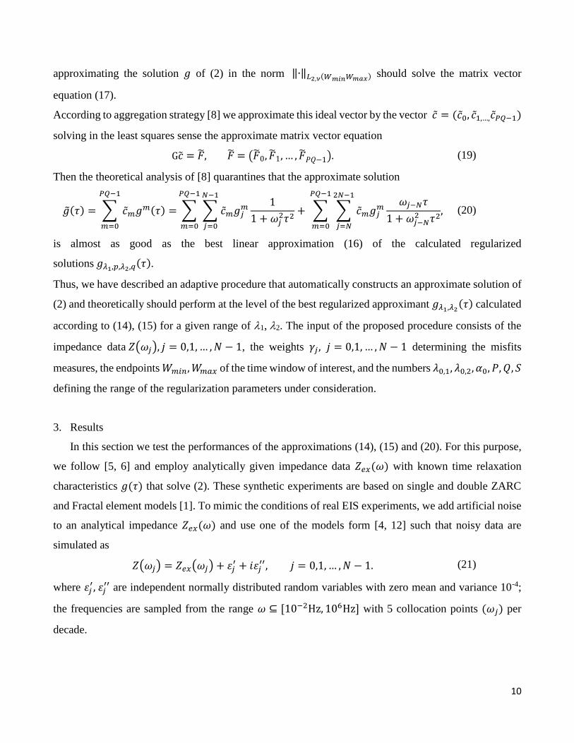
In Fig. 1 we plot DFRT 𝛾(𝜏) = 𝜏𝑔(𝜏) and the corresponding point values of its approximation

𝛾𝜆1,𝜆2(𝜏) = 𝜏𝑔𝜆1,𝜆2(𝜏) with best-turned parameters 𝜆1, 𝜆2.

12

Fig. 1. Exact (—) DFRT of single ZARC element model and the corresponding approximation (·) with best-tuned

parameters λ1, λ2.

Note that the above results and the ones reported below are obtained when in (15) the data misfits weights

𝛾𝑘 are chosen as

𝛾𝑘 = |𝑍(𝜔𝑘)|−2, 𝑘 = 0,1, … ,𝑁 − 1.

Such a choice has been advocated, for example, in [20].

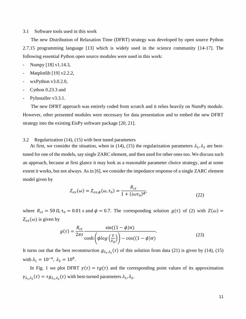
In the next synthetic experiment we simulate noisy data (21) from single Fractal element model,

where

𝑍𝑒𝑥(𝜔) = 𝑍𝑒𝑥,𝜙(𝜔, 𝜏0) =𝑅𝑐𝑡

(1 + 𝑖𝜔𝜏0)𝜙, (24)

and 𝑅𝑐𝑡, τ0 and 𝜙 are the same as in (22). Then the simulated data (21), (22) are used in the multi-

parameter regularization (14), (15) with the same values 𝜆1, 𝜆2 that were best-tuned for the single ZARC

element model (21), (22). The results are plotted in Fig. 2

Figure 2. Exact (—) DFRT of single Fractal element model and the corresponding computed approximation (·) with

parameters λ1, λ2, which are best-tuned for a single ZARC element model).

13

In Fig 2 the displayed oscillation in values of 𝛾𝜆1,𝜆2(𝜏) = 𝜏𝑔𝜆1,𝜆2(𝜏) for 𝜏 > 𝜏0 > 0.01(𝑠) can be

explained by the fact that in this experiment the corresponding exact solution

𝑔(𝜏) = {

𝑅𝑐𝑡𝜋

sin(𝜙𝜋)

𝜏1−𝜙(𝜏0 − 𝜏)𝜙 , 𝑖𝑓 𝜏 < 𝜏0

0, 𝑖𝑓 𝜏 > 𝜏0,

(25)

of the equation (2) has essential singularity not only at 𝜏 = 0 but also at 𝜏 = 𝜏0. Therefore, such

oscillations are common for other regularization techniques as well (see, e.g., [5]). On the other hand,

Fig. 2 shows that for 𝜏 < 𝜏0 the approximation provided by 𝜆1, 𝜆2, that were best-tuned for single ZARC

element model, is also quite good for the single Fractal element model.

At the same time, as we can see in the next example, it is not always reasonable to choose the

regularization parameters 𝜆1, 𝜆2 a priori.

Consider synthetic data (21) simulated from a double ZARC element model, where

𝑍𝑒𝑥(𝜔) = 𝑍𝑒𝑥,𝜙(𝜔, 𝜏0,1) + 𝑍𝑒𝑥,𝜙(𝜔, 𝜏0,2), (26)

and the summands in (26) are given by (22) with 𝜏0 = 𝜏0,1 = 0.01 (𝑠), 𝜏0 = 𝜏0,2 = 0.001 (𝑠). It is clear

that the corresponding exact solution of (2) is just a sum of two functions (23) with 𝜏0 = 𝜏0,1, 𝜏0,2. If we

now take the previous values of 𝜆1, 𝜆2 and apply regularization (14), (15) to the data (21), (26), then we

obtain the result displayed in Fig. 3, which does not allow a proper detection of the numbers of different

time constants (peaks) and their values (location) 𝜏0,1, 𝜏0,2. This example, provides a motivation for

employing the aggregation procedure described in Section 2.2.

Fig. 3. Exact (—) DFRT of double ZARC element model and the corresponding computed approximation (·) with

parameters λ1, λ2, which are best-tuned for a single ZARC element model.

14

3.3 Performance of the aggregated approximation (20)

The aggregation procedure resulting in the approximation (20), is illustrated with the following

values of the input parameters:

𝜆1,𝑝 = 10𝑝−7, 𝑝 = 0,1,2; 𝜆2,𝑞 = 105+𝑞 , 𝑞 = 0,1,2, … ,5;

𝛼𝑠 = 𝛼0𝛽𝑠, 𝑠 = 0,1,2, … ,9; 𝛼0 = 3.2 ∙ 104, 𝛽 = 0.2 ;

𝑊𝑚𝑖𝑛 = 10−2,𝑊𝑚𝑎𝑥 = 102.

This means that altogether, 28 regularized approximate solutions (14), (15) need to be computed for each

collocation dataset {𝑍(𝜔𝑗)}, among them 18 approximants 𝑔𝜆1,𝜆2with 𝜆1 = 𝜆1,𝑝, 𝜆2 = 𝜆2,𝑞 are aggregated

in (20), and the remaining 10 approximants 𝑔𝜆1,𝜆2with 𝜆1 = 0, 𝜆2 = 𝛼𝑠 are used as 𝑓𝑠 = 𝑔0,𝛼𝑠 for

defining a vector �̃� in (19).

The illustration of the aggregation procedure is produced for two collocation datasets. One of them

has been simulated from a double ZARC element model and discussed in the previous subsection as a

motivation for the use of the aggregation procedure. The second one is simulated from a double Fractal

element model in the same way as (21), (26). The only difference is that this time the summands in (26)

are given by (24) with 𝜏0 = 𝜏0,1, 𝜏0,2. The inputs described above are used in the aggregation procedure

from Section 2.2. The aggregation is performed in the weighted norms ‖∙‖𝐿2,𝜈(𝑊𝑚𝑖𝑛𝑊𝑚𝑎𝑥) with the

weights 𝜌(𝜏) = 𝜏𝜈 , 𝜈 = 0,1,2. This means that three systems (19) need to be formed and solved (one for

each 𝜈) to find the coeficients 𝑔𝑗𝑛in (20). Note that no additional regularized approximants are computed

for this. The results are displayed in Fig. 4 (double ZARC element model) and in Fig. 5 (double Fractal

element model).

15

Fig. 4. The synthetic impedance data of double ZARC element model (a) and corresponding exact (—) and the

approximated DFTR, produced by the aggregation in different norms (b-d). The synthetic data of single ZARC element is

presented in inset of subplot (a).

These results show that the aggregation performed in one of the considered norms (‖∙‖𝐿2,2in the case

of ZARC, and ‖∙‖𝐿2,0 in the case of Fractal) does not produce good approximation and differs essentially

from the other ones.

Fig. 5. The synthetic impedance data of double Fractal element model (a) and corresponding exact (—) and the

approximated DFTR, produced by the aggregation in different norms (b-d).

16

At the same time, for two other norms the aggregation results are very similar and quite accurate.

This observation hints at the possibility that the approximations produced by the aggregation in different

norms can be seen as a kind of “expert opinions”. Then the decision upon the output of the whole

aggregation procedure can be made by “majority voting”.

In Fig. 5 one can see the result of the regularization (14), (15) corresponds to the values 𝜆1 =

10−6, 𝜆2 = 1010 that are the best tuned to the reconstruction from the considered data, which have been

simulated from double Fractal element model. This result is quite similar to the one obtained in the

aggregation after the above mentioned “majority voting” and supports the theoretical claim that the

aggregated approximant (20) is almost as good as the best approximant involved in the aggregation

procedure.

At the end, we would like to highlight one more feature of the aggregated approximation (20), namely

its ability to properly determine the number of time constants involved in the models under consideration

(i.e. the peaks in DFTR shapes) from similar looking impedance spectra.

To illustrate this, we observe that the impedance spectra of single and double ZARC element models

(inset in Fig. 4a and Fig. 4a) look very similar, such that their visual inspection does not reveal a

difference in numbers of peaks of corresponding DFRT shapes. At the same time, the aggregation

procedure resulting in the approximation (20) automatically detects the above mentioned difference (see

right panels of Fig. 1 and Fig. 4bc) without any changes in input parameters 𝜆1,𝑝, 𝜆2,𝑔, 𝛼𝑠, 𝑊𝑚𝑖𝑛,𝑊𝑚𝑎𝑥.

4. Conclusion

In this article, we have proposed a novel scheme for estimating DFRT based on multi-penalty

regularization. The performance of the proposed scheme depends on the choice of involved

regularization parameters.

The usual approach to such a choice is to compute approximate solutions for several parameter values

and then select only one of them according to some criterion. In this article we have followed another

strategy and employed a recent idea [8, 11] that uses all computed approximate solutions to construct a

new one performing at the level of the best, but unknown, computed approximation.

The application of this idea is not restricted to the proposed scheme. A possible scenario may be the

combination of different approximations, such as [3-5], by using the same aggregation strategy.

Another novelty of the article is the observation that no additional discretization is necessary when

dealing with collocated equations of DFRT problem. This observation allows direct implementation of

17

the proposed multi-penalty regularization scheme such that all appearing quantities, except design

parameters, can be calculated exactly/symbolically. Based on our discussion of the synthetic

experiments, we conclude that the proposed scheme exhibits expected performance and can be

implemented in the form of a toolbox.

With intention to enable wider usage of the toolbox, it has been embedded in the free EisPy v.3.01

software package which is openly shared online [22] under the MIT license1.

Acknowledgments

M.Ž gratefully acknowledges the stimulation program "Joint Excellence in Science and Humanities"

(JESH) of the Austrian Academy of Sciences for providing supporting funds. S.P.Jr. acknowledges the

support of Austrian Science Fund (FWF), Project P 29514. Both authors express their gratitude to Prof.

Dr. Sergei Pereverzyev (the JESH-host scientist at RICAM) for fruitful suggestions and valuable

comments.

5. References

[1] E. Barsoukov, J.R. Macdonald, Impedance Spectroscopy: Theory, Experiment, and Applications,

2005.

[2] F. Dion, A. Lasia, The use of regularization methods in the deconvolution of underlying distributions

in electrochemical processes, Journal of Electroanalytical Chemistry 475(1) (1999) 28-37.

[3] R.A. Renaut, R. Baker, M. Horst, C. Johnson, D. Nasir, Stability and error analysis of the polarization

estimation inverse problem for microbial fuel cells, Inverse Problems 29(4) (2013).

[4] A.L. Gavrilyuk, D.A. Osinkin, D.I. Bronin, The Use of Tikhonov Regularization Method for

Calculating the Distribution Function of Relaxation Times in Impedance Spectroscopy, Russian Journal

of Electrochemistry 53(6) (2017) 575-588.

[5] M. Saccoccio, T.H. Wan, C. Chen, F. Ciucci, Optimal Regularization in Distribution of Relaxation

Times applied to Electrochemical Impedance Spectroscopy: Ridge and Lasso Regression Methods - A

Theoretical and Experimental Study, Electrochimica Acta 147 (2014) 470-482.

1 See: https://opensource.org/licenses/MIT.

18

[6] T.H. Wan, M. Saccoccio, C. Chen, F. Ciucci, Influence of the Discretization Methods on the

Distribution of Relaxation Times Deconvolution: Implementing Radial Basis Functions with DRTtools,

Electrochimica Acta 184 (2015) 483-499.

[7] P. Mathe, S.V. Pereverzev, Discretization strategy for linear ill-posed problems in variable Hilbert

scales, Inverse Problems 19(6) (2003) 1263-1277.

[8] J.Y. Chen, S. Pereverzyev, Y.S. Xu, Aggregation of regularized solutions from multiple observation

models, Inverse Problems 31(7) (2015).

[9] K.S. Cole, R.H. Cole, Dispersion and absorption in dielectrics I. Alternating current characteristics,

Journal of Chemical Physics 9(4) (1941) 341-351.

[10] L.D.K. (originator), Encyclopedia of Mathematics : Weighted space, 1993.

http://www.encyclopediaofmath.org/index.php?title=Weighted_space&oldid=15433.

[11] S. Kindermann, S. Pereverzyev, Jr., A. Pilipenko, The quasi-optimality criterion in the linear

functional strategy, ArXiv e-prints, 2017.

[12] F. Ciucci, C. Chen, Analysis of Electrochemical Impedance Spectroscopy Data Using the

Distribution of Relaxation Times: A Bayesian and Hierarchical Bayesian Approach, Electrochimica Acta

167 (2015) 439-454.

[13] T.E. Oliphant, Python for scientific computing, Computing in Science & Engineering 9(3) (2007)

10-20.

[14] D.S. Cao, Q.S. Xu, Q.N. Hu, Y.Z. Liang, ChemoPy: Freely available python package for

computational biology and chemoinformatics, Bioinformatics 29(8) (2013) 1092-1094.

[15] J.J. Helmus, C.P. Jaroniec, Nmrglue: An open source Python package for the analysis of

multidimensional NMR data, Journal of Biomolecular NMR 55(4) (2013) 355-367.

[16] D.S. Cao, Q.S. Xu, Y.Z. Liang, Propy: A tool to generate various modes of Chou's PseAAC,

Bioinformatics 29(7) (2013) 960-962.

[17] J. Kieffer, J.P. Wright, PyFAI: A python library for high performance azimuthal integration on GPU,

Powder Diffraction 28(SUPPL.2) (2013) S339-S350.

[18] S. van der Walt, S.C. Colbert, G. Varoquaux, The NumPy Array: A Structure for Efficient Numerical

Computation, Computing in Science & Engineering 13(2) (2011) 22-30.

[19] J.D. Hunter, Matplotlib: A 2D graphics environment, Computing in Science & Engineering 9(3)

(2007) 90-95.

19

[20] M. Zic, An alternative approach to solve complex nonlinear least-squares problems, Journal of

Electroanalytical Chemistry 760 (2016) 85-96.

[21] M. Zic, Solving CNLS problems by using Levenberg-Marquardt algorithm: A new approach to

avoid off-limits values during a fit, Journal of Electroanalytical Chemistry 799 (2017) 242-248.

[22] EisPy v.3.01 is hosted on https://goo.gl/j5nizb.