SIViP (2016) 10:663–670DOI 10.1007/s11760-015-0791-3

ORIGINAL PAPER

Adaptive Kuwahara filter

Krzysztof Bartyzel1

Received: 15 September 2014 / Revised: 12 June 2015 / Accepted: 18 June 2015 / Published online: 6 July 2015© The Author(s) 2015. This article is published with open access at Springerlink.com

Abstract A new filter was created by improving the stan-dard Kuwahara filter. It allows more efficient noise reductionwithout blurring the edges and imagepreparation for segmen-tation and further analyses operations. One of the biggest andmost common restrictions encountered in filter algorithmsis the need for a declarative definition of the filter windowsize or the number of iterations that an operation should berepeated. In the case of the proposed solution, we are deal-ing with automatic adaptation of the algorithm to the localenvironment of each pixel in the processed image.

Keywords Noise reduction · Image processing ·Image filtering

1 Introduction

Contextual transformations are operations in which the out-come depends on amodified pixel and its surroundings [4,5].Alternatively, the name “digital filters” is also used. Theapplication of digital filters is very wide, and they are usedin many areas of life including radiology, automatic controlsystems andmachine vision. Themain applications of digitalfilters are as follows:

• suppressing unwanted noise,• improving image sharpness,• removing specific defects ,• visualizing certain image features,• reconstructing partly destroyed images.

B Krzysztof Bartyzelkrzysztof.bartyzel@gmail.com

1 Department of Computer Image Analysis, John Paul IICatholic University of Lublin, al. Racławickie 14, 20-950Lublin, Poland

In this paper, I address the issues of reducing noise fromdigital images and present a new highly efficient algorithm.The issue of noise or other errors is extremely importantbecause they can appear during image acquisition, transmis-sion or compression and decompression. Therefore, imagefiltering is a very important aspect of image processing andpreparation for further work such as image compression,edge detection or image segmentation. The application ofnoise reduction algorithms is also extensively used inmedicalimaging. A large number of articles discussing this subjecthave been published, e.g., [2,3].

However, at the beginning I would like to present the pre-sentation of the standard commonly used algorithms and toclarify the terms used.

It is highly likely that there exist filters that remove noisefrom digital images faster, gain a better rate of bug fixingor modify the edges of objects less than those used in thisstudy. However, a comparison of all the existing solutionswould require a large and difficult to estimate amount ofwork, at least because of the need to provide a similar levelof implementation and other conditions of the experiment,and thus, it would exceed significantly the planned scope ofthe study. There is nothing, however, to prevent extending thescope of the comparison and to present its results in futurepublications.

The general concept of the context filters is to create theoutput image on the basis of the source image in such a waythat the value of each pixel at coordinates (x,y) in the outputimage is determined based on a certain neighborhood of thepixel at coordinates (x,y) in the source image [4–9]. Thisneighborhood is defined as a filter window. Usually, it isassumed that the filter window is square and the size (widthandheight) is an odd integer number, e.g., 3×3, 5×5, 7×7. Inthis case, a pixel at coordinates (x,y) is exactly in the middleof the filter window. There are also solutions that collect

123

664 SIViP (2016) 10:663–670

statistical information about the entire image and then usethem during the processing of each pixel.

2 Context filters

2.1 Average filter

The average filter is one of the simplest filters enablingremoving noise and distortion. Unfortunately, it also intro-duces changes in the areas that have originally been noiseand distortion free.

Let us assume that we construct a filter operating on thewindow N × N . In this case, the resulting value of the pixelis the average value of all the pixels contained within thecurrent analysis window of the source image

mθ = 1

N × N×

∑

(x,y)∈θ

ϕ(f (x, y)

)(1)

where:

f is the source image function,f (x,y) is the value of the pixel at coordinates (x, y),ϕ is a function calculating the value of a particular pixel.This function can take different values depending on thecolor space, the format or the depth of the image,N × N is the number of pixels in the current window,θ represents the collection of pixels in the current win-dow.

Some of the largest disadvantages of the average filter areblurring noise and significant modification of correct pixels.

2.2 Median filter

The concept of the median filter is very similar to that shownabove. The only difference is that all elements in the currentfilter window have to be sorted and ordered in an ascendingsequence. The resulting value is the value of the item in theexact middle point of the ordered sequence (position N×N

2for N × N window).

With the use of this filter, one can very effectively removeany local noise, without blurring the noise to larger areas,which was a major disadvantage of the average filter.

2.3 Adaptive median filter

The adaptive median filter, as its name suggests, is a mod-ification of the median filter. This modification consists inallowing a situation where the window size is not constant,but changes dynamically according to the context. If youselect too small a window, the median filter could not handle

all the noises, while too large a window results in dissolvingthe smaller but desired image detail.

The adaptive median filter algorithm has the followingform:

Step 1 For each pixel f (x, y) of the image f, we determinethe list of neighbors in N × N window. Among these ele-ments, we calculate the minimum, middle (median) and themaximum value and denote these values as fmin, fmed andfmax, respectively.

Step 2 If fmin = fmed or fmed = fmax, then the size of filterwindow is increasing and the actions done in the previousstep for the new window have to be repeated. Otherwise, goto the next step.

For obvious reasons, theremust exist themaximum allow-able window size. If it is not possible to further increase thefilter window size, then the output pixel is set to the neighborslist middle value determined in the previous step ( fmed).

Step 3 If fmin < f (x, y) and f (x, y) < fmax, then theoutput pixel takes the value of f (x, y), which means thatitem is not modified. Otherwise, the output pixel is set tothe neighbors list middle value determined in the first step( fmed).

This filter is able to reduce even a large noise. Unfor-tunately, the high computational complexity of this filter isquite a serious disadvantage. In addition, if the maximumwindow size is set to too small a value, we can get unsatis-factory results. However, too large a window size may causevery unsatisfactory execution time.

2.4 Kuwahara filter

Because the contour plays a very important role in theprocess of image analysis [4,9], it is very important toensure that the image smoothing does not affect the sharp-ness of contours. This could cause serious problems later,during segmentation. The Kuwahara filter [1] is an exam-ple of a filter which meets these requirements. This filtercan be constructed for any window size. For readability,the algorithm will be described for the window of size of3 × 3.

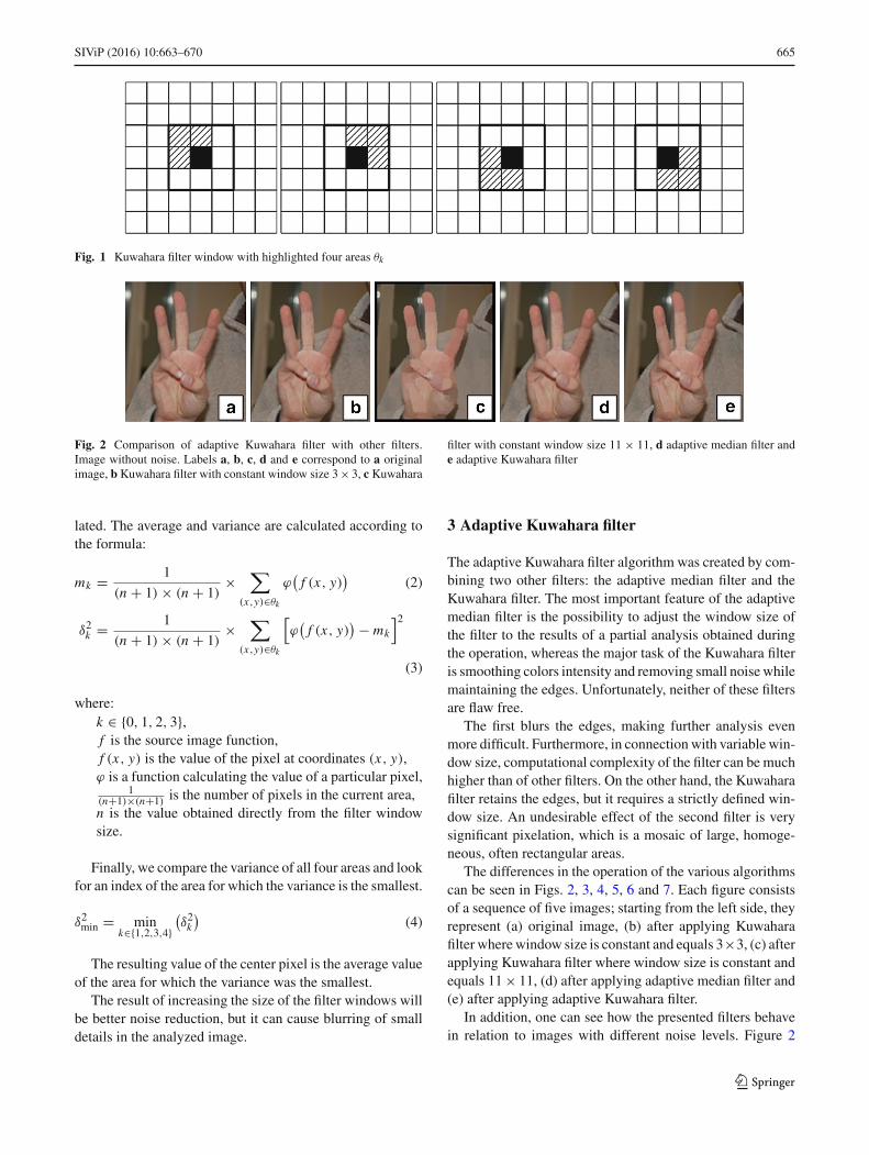
The filter window should be divided into four areas.Let us denote them as θk where k ∈ {0, 1, 2, 3}. Thesefour areas are highlighted in Fig. 1. The center pixel ismarked with black color. If a square filter window con-sists of (2 × n + 1) × (2 × n + 1) elements, then eacharea will contain exactly (n + 1) × (n + 1) elements. Inthe described case, the filter window size is 3 × 3, so eacharea will consist of four elements. Then, for each of theseareas, the values of average mk and variance δ2k are calcu-

123

SIViP (2016) 10:663–670 665

Fig. 1 Kuwahara filter window with highlighted four areas θk

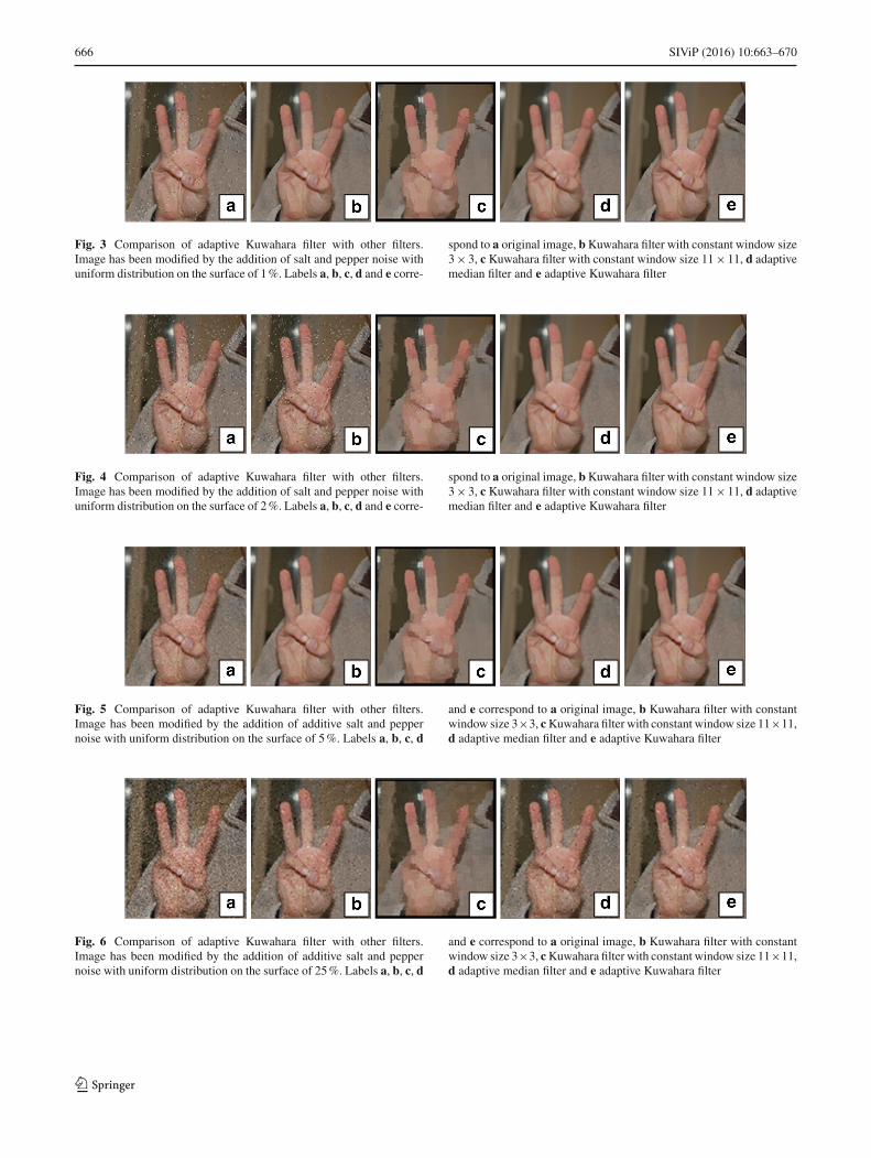
Fig. 2 Comparison of adaptive Kuwahara filter with other filters.Image without noise. Labels a, b, c, d and e correspond to a originalimage, bKuwahara filter with constant window size 3× 3, c Kuwahara

filter with constant window size 11 × 11, d adaptive median filter ande adaptive Kuwahara filter

lated. The average and variance are calculated according tothe formula:

mk = 1

(n + 1) × (n + 1)×

∑

(x,y)∈θk

ϕ(f (x, y)

)(2)

δ2k = 1

(n + 1) × (n + 1)×

∑

(x,y)∈θk

[ϕ(f (x, y)

) − mk

]2

(3)

where:k ∈ {0, 1, 2, 3},f is the source image function,f (x, y) is the value of the pixel at coordinates (x, y),ϕ is a function calculating the value of a particular pixel,

1(n+1)×(n+1) is the number of pixels in the current area,n is the value obtained directly from the filter windowsize.

Finally, we compare the variance of all four areas and lookfor an index of the area for which the variance is the smallest.

δ2min = mink∈{1,2,3,4}

(δ2k

)(4)

The resulting value of the center pixel is the average valueof the area for which the variance was the smallest.

The result of increasing the size of the filter windows willbe better noise reduction, but it can cause blurring of smalldetails in the analyzed image.

3 Adaptive Kuwahara filter

The adaptive Kuwahara filter algorithm was created by com-bining two other filters: the adaptive median filter and theKuwahara filter. The most important feature of the adaptivemedian filter is the possibility to adjust the window size ofthe filter to the results of a partial analysis obtained duringthe operation, whereas the major task of the Kuwahara filteris smoothing colors intensity and removing small noise whilemaintaining the edges. Unfortunately, neither of these filtersare flaw free.

The first blurs the edges, making further analysis evenmore difficult. Furthermore, in connection with variable win-dow size, computational complexity of the filter can be muchhigher than of other filters. On the other hand, the Kuwaharafilter retains the edges, but it requires a strictly defined win-dow size. An undesirable effect of the second filter is verysignificant pixelation, which is a mosaic of large, homoge-neous, often rectangular areas.

The differences in the operation of the various algorithmscan be seen in Figs. 2, 3, 4, 5, 6 and 7. Each figure consistsof a sequence of five images; starting from the left side, theyrepresent (a) original image, (b) after applying Kuwaharafilter wherewindow size is constant and equals 3×3, (c) afterapplying Kuwahara filter where window size is constant andequals 11× 11, (d) after applying adaptive median filter and(e) after applying adaptive Kuwahara filter.

In addition, one can see how the presented filters behavein relation to images with different noise levels. Figure 2

123

666 SIViP (2016) 10:663–670

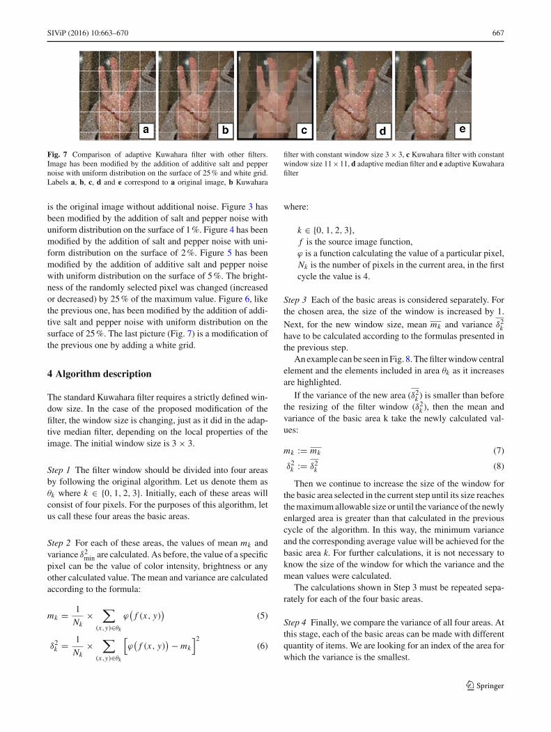
Fig. 3 Comparison of adaptive Kuwahara filter with other filters.Image has been modified by the addition of salt and pepper noise withuniform distribution on the surface of 1%. Labels a, b, c, d and e corre-

spond to a original image, bKuwahara filter with constant window size3× 3, c Kuwahara filter with constant window size 11× 11, d adaptivemedian filter and e adaptive Kuwahara filter

Fig. 4 Comparison of adaptive Kuwahara filter with other filters.Image has been modified by the addition of salt and pepper noise withuniform distribution on the surface of 2%. Labels a, b, c, d and e corre-

spond to a original image, bKuwahara filter with constant window size3× 3, c Kuwahara filter with constant window size 11× 11, d adaptivemedian filter and e adaptive Kuwahara filter

Fig. 5 Comparison of adaptive Kuwahara filter with other filters.Image has been modified by the addition of additive salt and peppernoise with uniform distribution on the surface of 5%. Labels a, b, c, d

and e correspond to a original image, b Kuwahara filter with constantwindow size 3×3, cKuwahara filter with constant window size 11×11,d adaptive median filter and e adaptive Kuwahara filter

Fig. 6 Comparison of adaptive Kuwahara filter with other filters.Image has been modified by the addition of additive salt and peppernoise with uniform distribution on the surface of 25%. Labels a, b, c, d

and e correspond to a original image, b Kuwahara filter with constantwindow size 3×3, cKuwahara filter with constant window size 11×11,d adaptive median filter and e adaptive Kuwahara filter

123

SIViP (2016) 10:663–670 667

Fig. 7 Comparison of adaptive Kuwahara filter with other filters.Image has been modified by the addition of additive salt and peppernoise with uniform distribution on the surface of 25% and white grid.Labels a, b, c, d and e correspond to a original image, b Kuwahara

filter with constant window size 3× 3, c Kuwahara filter with constantwindow size 11×11, d adaptive median filter and e adaptive Kuwaharafilter

is the original image without additional noise. Figure 3 hasbeen modified by the addition of salt and pepper noise withuniform distribution on the surface of 1%. Figure 4 has beenmodified by the addition of salt and pepper noise with uni-form distribution on the surface of 2%. Figure 5 has beenmodified by the addition of additive salt and pepper noisewith uniform distribution on the surface of 5%. The bright-ness of the randomly selected pixel was changed (increasedor decreased) by 25% of the maximum value. Figure 6, likethe previous one, has been modified by the addition of addi-tive salt and pepper noise with uniform distribution on thesurface of 25%. The last picture (Fig. 7) is a modification ofthe previous one by adding a white grid.

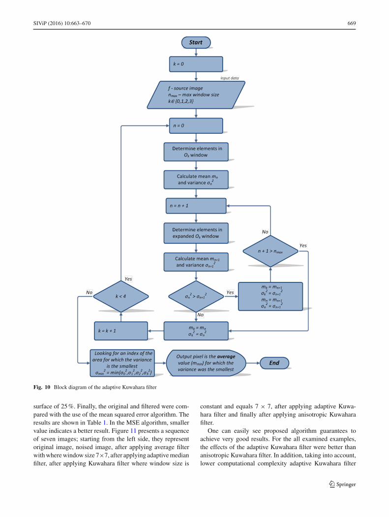
4 Algorithm description

The standard Kuwahara filter requires a strictly defined win-dow size. In the case of the proposed modification of thefilter, the window size is changing, just as it did in the adap-tive median filter, depending on the local properties of theimage. The initial window size is 3 × 3.

Step 1 The filter window should be divided into four areasby following the original algorithm. Let us denote them asθk where k ∈ {0, 1, 2, 3}. Initially, each of these areas willconsist of four pixels. For the purposes of this algorithm, letus call these four areas the basic areas.

Step 2 For each of these areas, the values of mean mk andvariance δ2min are calculated. As before, the value of a specificpixel can be the value of color intensity, brightness or anyother calculated value. The mean and variance are calculatedaccording to the formula:

mk = 1

Nk×

∑

(x,y)∈θk

ϕ(f (x, y)

)(5)

δ2k = 1

Nk×

∑

(x,y)∈θk

[ϕ(f (x, y)

) − mk

]2(6)

where:

k ∈ {0, 1, 2, 3},f is the source image function,ϕ is a function calculating the value of a particular pixel,Nk is the number of pixels in the current area, in the firstcycle the value is 4.

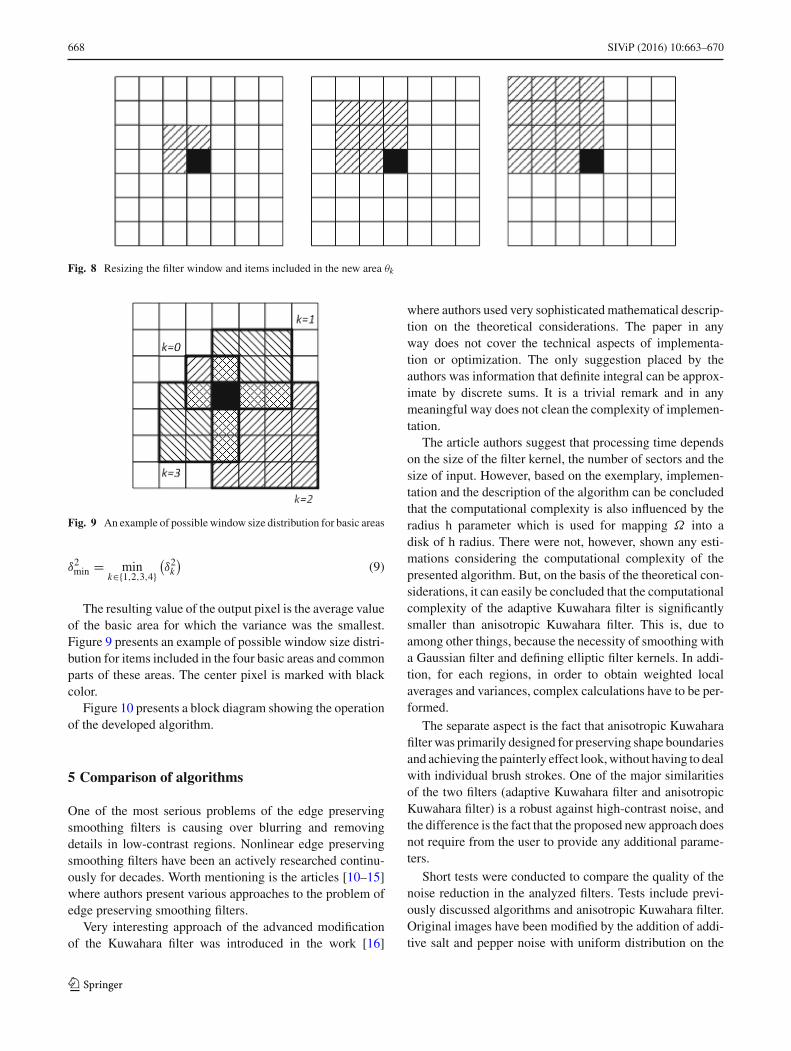
Step 3 Each of the basic areas is considered separately. Forthe chosen area, the size of the window is increased by 1.

Next, for the new window size, mean mk and variance δ2khave to be calculated according to the formulas presented inthe previous step.

Anexample canbe seen inFig. 8. Thefilterwindowcentralelement and the elements included in area θk as it increasesare highlighted.

If the variance of the new area (δ2k ) is smaller than beforethe resizing of the filter window (δ2k ), then the mean andvariance of the basic area k take the newly calculated val-ues:

mk := mk (7)

δ2k := δ2k (8)

Then we continue to increase the size of the window forthe basic area selected in the current step until its size reachesthemaximumallowable size or until the variance of the newlyenlarged area is greater than that calculated in the previouscycle of the algorithm. In this way, the minimum varianceand the corresponding average value will be achieved for thebasic area k. For further calculations, it is not necessary toknow the size of the window for which the variance and themean values were calculated.

The calculations shown in Step 3 must be repeated sepa-rately for each of the four basic areas.

Step 4 Finally, we compare the variance of all four areas. Atthis stage, each of the basic areas can be made with differentquantity of items. We are looking for an index of the area forwhich the variance is the smallest.

123

668 SIViP (2016) 10:663–670

Fig. 8 Resizing the filter window and items included in the new area θk

Fig. 9 An example of possible window size distribution for basic areas

δ2min = mink∈{1,2,3,4}

(δ2k

)(9)

The resulting value of the output pixel is the average valueof the basic area for which the variance was the smallest.Figure 9 presents an example of possible window size distri-bution for items included in the four basic areas and commonparts of these areas. The center pixel is marked with blackcolor.

Figure 10 presents a block diagram showing the operationof the developed algorithm.

5 Comparison of algorithms

One of the most serious problems of the edge preservingsmoothing filters is causing over blurring and removingdetails in low-contrast regions. Nonlinear edge preservingsmoothing filters have been an actively researched continu-ously for decades. Worth mentioning is the articles [10–15]where authors present various approaches to the problem ofedge preserving smoothing filters.

Very interesting approach of the advanced modificationof the Kuwahara filter was introduced in the work [16]

where authors used very sophisticatedmathematical descrip-tion on the theoretical considerations. The paper in anyway does not cover the technical aspects of implementa-tion or optimization. The only suggestion placed by theauthors was information that definite integral can be approx-imate by discrete sums. It is a trivial remark and in anymeaningful way does not clean the complexity of implemen-tation.

The article authors suggest that processing time dependson the size of the filter kernel, the number of sectors and thesize of input. However, based on the exemplary, implemen-tation and the description of the algorithm can be concludedthat the computational complexity is also influenced by theradius h parameter which is used for mapping Ω into adisk of h radius. There were not, however, shown any esti-mations considering the computational complexity of thepresented algorithm. But, on the basis of the theoretical con-siderations, it can easily be concluded that the computationalcomplexity of the adaptive Kuwahara filter is significantlysmaller than anisotropic Kuwahara filter. This is, due toamong other things, because the necessity of smoothing witha Gaussian filter and defining elliptic filter kernels. In addi-tion, for each regions, in order to obtain weighted localaverages and variances, complex calculations have to be per-formed.

The separate aspect is the fact that anisotropic Kuwaharafilter was primarily designed for preserving shape boundariesand achieving the painterly effect look,without having to dealwith individual brush strokes. One of the major similaritiesof the two filters (adaptive Kuwahara filter and anisotropicKuwahara filter) is a robust against high-contrast noise, andthe difference is the fact that the proposed new approach doesnot require from the user to provide any additional parame-ters.

Short tests were conducted to compare the quality of thenoise reduction in the analyzed filters. Tests include previ-ously discussed algorithms and anisotropic Kuwahara filter.Original images have been modified by the addition of addi-tive salt and pepper noise with uniform distribution on the

123

SIViP (2016) 10:663–670 669

Fig. 10 Block diagram of the adaptive Kuwahara filter

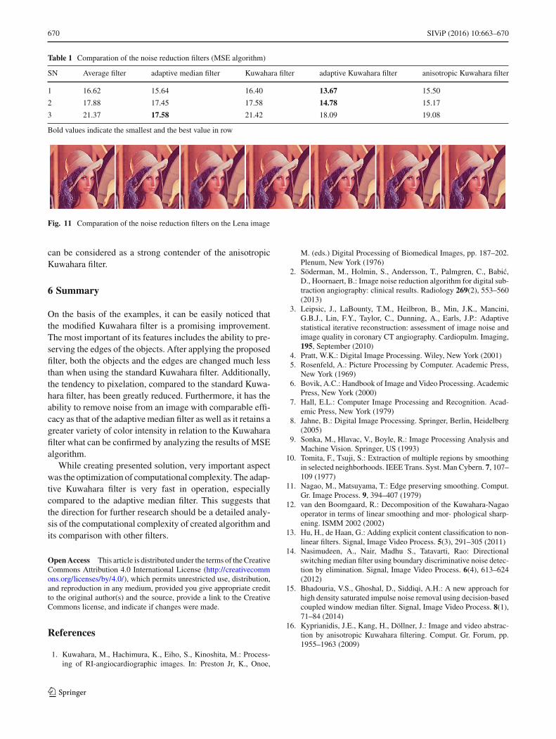
surface of 25%. Finally, the original and filtered were com-pared with the use of the mean squared error algorithm. Theresults are shown in Table 1. In the MSE algorithm, smallervalue indicates a better result. Figure 11 presents a sequenceof seven images; starting from the left side, they representoriginal image, noised image, after applying average filterwithwherewindow size 7×7, after applying adaptivemedianfilter, after applying Kuwahara filter where window size is

constant and equals 7 × 7, after applying adaptive Kuwa-hara filter and finally after applying anisotropic Kuwaharafilter.

One can easily see proposed algorithm guarantees toachieve very good results. For the all examined examples,the effects of the adaptive Kuwahara filter were better thananisotropic Kuwahara filter. In addition, taking into account,lower computational complexity adaptive Kuwahara filter

123

670 SIViP (2016) 10:663–670

Table 1 Comparation of the noise reduction filters (MSE algorithm)

SN Average filter adaptive median filter Kuwahara filter adaptive Kuwahara filter anisotropic Kuwahara filter

1 16.62 15.64 16.40 13.67 15.50

2 17.88 17.45 17.58 14.78 15.17

3 21.37 17.58 21.42 18.09 19.08

Bold values indicate the smallest and the best value in row

Fig. 11 Comparation of the noise reduction filters on the Lena image

can be considered as a strong contender of the anisotropicKuwahara filter.

6 Summary

On the basis of the examples, it can be easily noticed thatthe modified Kuwahara filter is a promising improvement.The most important of its features includes the ability to pre-serving the edges of the objects. After applying the proposedfilter, both the objects and the edges are changed much lessthan when using the standard Kuwahara filter. Additionally,the tendency to pixelation, compared to the standard Kuwa-hara filter, has been greatly reduced. Furthermore, it has theability to remove noise from an image with comparable effi-cacy as that of the adaptive median filter as well as it retains agreater variety of color intensity in relation to the Kuwaharafilter what can be confirmed by analyzing the results of MSEalgorithm.

While creating presented solution, very important aspectwas the optimization of computational complexity. The adap-tive Kuwahara filter is very fast in operation, especiallycompared to the adaptive median filter. This suggests thatthe direction for further research should be a detailed analy-sis of the computational complexity of created algorithm andits comparison with other filters.

OpenAccess This article is distributed under the terms of theCreativeCommons Attribution 4.0 International License (http://creativecommons.org/licenses/by/4.0/), which permits unrestricted use, distribution,and reproduction in any medium, provided you give appropriate creditto the original author(s) and the source, provide a link to the CreativeCommons license, and indicate if changes were made.

References

1. Kuwahara, M., Hachimura, K., Eiho, S., Kinoshita, M.: Process-ing of RI-angiocardiographic images. In: Preston Jr, K., Onoe,

M. (eds.) Digital Processing of Biomedical Images, pp. 187–202.Plenum, New York (1976)

2. Söderman, M., Holmin, S., Andersson, T., Palmgren, C., Babic,D., Hoornaert, B.: Image noise reduction algorithm for digital sub-traction angiography: clinical results. Radiology 269(2), 553–560(2013)

3. Leipsic, J., LaBounty, T.M., Heilbron, B., Min, J.K., Mancini,G.B.J., Lin, F.Y., Taylor, C., Dunning, A., Earls, J.P.: Adaptivestatistical iterative reconstruction: assessment of image noise andimage quality in coronary CT angiography. Cardiopulm. Imaging,195, September (2010)

4. Pratt, W.K.: Digital Image Processing. Wiley, New York (2001)5. Rosenfeld, A.: Picture Processing by Computer. Academic Press,

New York (1969)6. Bovik, A.C.: Handbook of Image and Video Processing. Academic

Press, New York (2000)7. Hall, E.L.: Computer Image Processing and Recognition. Acad-

emic Press, New York (1979)8. Jahne, B.: Digital Image Processing. Springer, Berlin, Heidelberg

(2005)9. Sonka, M., Hlavac, V., Boyle, R.: Image Processing Analysis and

Machine Vision. Springer, US (1993)10. Tomita, F., Tsuji, S.: Extraction of multiple regions by smoothing

in selected neighborhoods. IEEE Trans. Syst. Man Cybern. 7, 107–109 (1977)

11. Nagao, M., Matsuyama, T.: Edge preserving smoothing. Comput.Gr. Image Process. 9, 394–407 (1979)

12. van den Boomgaard, R.: Decomposition of the Kuwahara-Nagaooperator in terms of linear smoothing and mor- phological sharp-ening. ISMM 2002 (2002)

13. Hu, H., de Haan, G.: Adding explicit content classification to non-linear filters. Signal, Image Video Process. 5(3), 291–305 (2011)

14. Nasimudeen, A., Nair, Madhu S., Tatavarti, Rao: Directionalswitching median filter using boundary discriminative noise detec-tion by elimination. Signal, Image Video Process. 6(4), 613–624(2012)

15. Bhadouria, V.S., Ghoshal, D., Siddiqi, A.H.: A new approach forhigh density saturated impulse noise removal using decision-basedcoupled window median filter. Signal, Image Video Process. 8(1),71–84 (2014)

16. Kyprianidis, J.E., Kang, H., Döllner, J.: Image and video abstrac-tion by anisotropic Kuwahara filtering. Comput. Gr. Forum, pp.1955–1963 (2009)

123