Adaptive Histogram Equalization And Its Variations

July, 1986

Technical Report 86-013

Stephen M. Puer, E. Philip Amburn, John D. Austin, Roberl Cromartie, Ari Geselowit., 7rey Greer, Bart ter Haar Romeny, John

B. Zimmerman, and Karel Zuiderveld

The University of North Carolina at Chapel Hill Department of Computer Science New West Hall 035 A Chapel Hill, N.C. 27514

Submitted to Computer Vision, Graphics, and Im&Ke ProcessinK

j Submitted to Computer Vision, Graphics,

and Image Processing ·---

ADAPTIVE HISTOGRAM EQUALIZATION AND ITS VARIATIONS

Stephen M. Pizer*+, E. Philip Amburn**, John D. Austin*, Robert Cromartie*, Ari Geselowitzf, Trey Greer*, Bart ter Haar Romeny§,

John B. Zimmerman f, and Karel Zuiderveld§

Correspondence: Dr. Stephen M. Pizer Computer Science Department University of North Carolina 207A New West Hall 035A Chapel ffill, NC 27514

Department of Computer Science* and Department of Radiology +, University of North Carolina, Chapel Hill, NC, USA, United States Air Force*, School of Medicine t, Penn­sylvania State University, Hershey, PA, USA, Roentgenafdeling §, Academisch Zieken· huiz Utrecht, and Department of Computer Science f, Washington University, St. Louis, MO, USA.

,, ·.

Abstract

Adaptive histogram equalization (abe) is a contrast enhancement method designed to

be broadly applicable and having demonstrated effectiveness. However, slow speed and the

overenhancement of noise it produces in relatively homogeneous regions are two problems.

We report algorithms designed to overcome these and other concerns. These algorithms

include interpolated ahe, to speed up the method on general purpose computers; a version

of interpolated ahe designed to run in a few seconds on feedback processors; a version of

full ahe designed to run in under one second on custom VLSI hardware; weighted ahe,

designed to improve the quality of the result by emphasizing pixels' contribution to the

histogram in relation to their nearness to the result pixel; and clipped ahe, designed to

overcome the problem of overenhancement of noise contrast. We conclude that clipped ahe

should become a method of choice in medical imaging and probably also in other areas of

digital imaging, and that clipped ahe can be made adequately fast to be routinely applied

in the normal display sequence.

2

'' ·.

Mathematical Symbols

+

* • I

X

3

plus

minus

times, point on graph

point on graph

divided by

equals, is assigned

times

etc.

program segment delimiters

such that

co=ent delimiters

is a member of

less than or equal

greater than

•'

1. INTRODUCTION

Adaptive histogram equa.liza.tion ( a.he) is an excellent contrast enhancement method

for both natural images and medical and other initia.lly nonvisual images. In medical

imaging its automatic operation and effective presentation of a.ll contrast a.va.ila.ble in the

image data. make it a. competitor to the standard contrast enhancement method, interactive

intensity windowing. In fact, observer studies [Zimmerman, 1985; ter Ha.ar Romeny, 1985]

indicate that for certain image classes, intensity windowing has no significant a.dva.nta.ges

in local contrast presentation in a.ny contrast range, while a.he has a.dva.nta.ges of being

automatic and reproducible, and requiring the observer to examine only a. single image.

The basic form of the method was invented independently by Ketcham [1976], Hummel

[1977], and Pizer [1981]. In this basic form the method involves applying to each pixel the

histogram equalization mapping based on the pixels in a. region surrounding that pixel (its

contextual region). That is, each pixel is mapped to a.n intensity proportional to its rank

in the pixels surrounding it. But the basic method is slow, and under certain conditions

the enhanced image has undesirable features. Therefore, this paper presents algorithms

for a.he that increase its speed on various processors, and it presents variations on a.he that

are intended to improve the enhanced image, along with summaries of the effectiveness of

these variations.

2. SPEEDUP BY SAMPLING AND INTERPOLATION

In its basic form a.he requires time O(n2 (m + k)) for an n x n image with a range of k

intensity levels and an m x m contextual region size. A major speedup can be obtained by

calculating the desired mapping only at a sample of pixels and interpolating the mapping

between these sample locations. In our work the sample locations at which the mapping

is computed are on a. grid, and the resulting mapping a.t any pixel is interpolated from the

sample mappings at the four surrounding sample-grid pixels (see figure 1). Thus, if the

pixel mapped is at location (z, y) and has intensity i, and m+- is the mapping at the grid

pixel (z+,!l-) to the upper right of (z,y) and similarly with subscripts++,-+, and-­

for the mappings and locations of the grid pixels to the

lower right, lower left, and upper left respectively of(::, y), then the interpolated ahe reeult

is given by

· m(i) = a(bm++(i) + (1- b)m+_(i)] + (1- a](bm_+(i) + (1- b}m--(&1],

where a= (y- r-)/(Y+ - r-) and b = (::- ::-)/(::+ - ::-)·

Pixels in the borders of the image outside of the sample pixels need to be handled specially,

using linear interpolation of the mappings at the two closest points or, in the corners where

there is only a single close sample pixel, application of only one mapping.

* * * * (x_, y _) (x+' y_)

* * * * • (x,y)

* * * * (x_, Y+) (x+' y +)

* * * *

Figure 1. Sample points(*) for mapping computation, and evaluation point (•).

With such an interpolated ahe there are two parameters, the sise of the contextual

regions and the spacing of the sample grid. We will discuss each of these in turn.

5

2.1. Contextual Region Size

In the interpolative mapping procedure each result pixel is derived by applying four

mappings, those associated with four surrounding sample points. Each of those sample

points has an associated contextual region, so it can be said that the result pixel in question

has a region affecting its value that is the union of the four associated contextual regions

of its sample points. Let us call this affecting region the equivalent contextual region, or

ECR. We have found empirically (see figure 2) that different versions of the method with

the same ECR produce approximately the same result. Thus, for example, if the sample

grid point spacing is the same as the contextual region linear dimension, thus forming a

mosaic of contextual regions within the image (see figure 3a), then uninterpolated (basic)

ahe with contextual region area A (and thus ECR A) produces approximately the same

results as interpolated ahe with contextual region area A/4 (and thus ECR A). Similarly,

if the sample grid point spacing is half that of the contextual region linear dimension (see

section 2.2 and figure 3b}, interpolated ahe with contextual region area 4A/9 will produce

about the same result as the just mentioned two cases. As a result of this fact, we will

henceforth refer to sample-based methods in terms of their ECR.

Figure 2. Results for interpolative ahe of a chest CT scan, with the same ECR's. a) Full

sampling (no interpolation), b) Mosaic sampling.

6

As the ECR area increases, the method becomes less and less locally sensitive but for

interpolative abe more and more efficient As the ECR area decreases, the image contrast

improves up to a point For a wide range of medical images this optimal ECR area is

between 1/16 and 1/64 of the image, with the smaller region chosen only when the feature

size of interest is quite small. ECR areas intermediate between 1/16 and 1/64 of the

image area produce results not ~poriantly different from that using 1/16 of the image,

because the image appearance changes only slowly with ECR area. H the ECR is much

less than 1/64 of the image, the contrast becomes too sensitive to very local variations and

in particular to image noise. This oversensitivity to local variations can cause artifacts,

which have never been experienced with the preferred ECR's.

With these values for ECR interpolative abe of a 512 x 512 image requires less than.

two minutes for a C program on a VAX 11/780 or an assembly language program on a

small16-bit minicomputer. This is a savings of well over an order of magnitude over abe

with full sampling. ·

2.2. Contextual Region Sampling Rate

We have evaluated sampling in each dimension at a distance equal to the contextual

region linear dimension (so that the sample regions divide the image into a mosaic - see

figure 3a), at half this distance (see figure 3b), and at one pixel (full sampling). The

advantage of sampling at half the contextual linear dimension is that, unlike with mosaic

sampling, each pixel contributes to the histograms of all four sample contextual regions

whose mappings are applied to that pixel (Herman, 1984].

Of course, the coarser the sampling, the faster the results are computed. Although test

pattern images can be created where finer than mosaic sampling is desirable to produce

adequate quality, we have never found an image of the complexity of clinical medical images

for which mosaic sampling was not effectively equivalent to the finer sampling for the same

ECR.

7

-

•

* * * *

* ·* * * a)

* * * *

* * * *

* ) * ) •' * !

* ..... ...:·· ·- .. .. .. >.<

0

.W. -~ ~ ~ .,. .,, .,, . .,

* . --~ -· * .. ··' . * ..,:,.

* -. , -. ... 0

b) "' "' ·" .: .. ,,, . ' ..... . ' .... .,

'!'

* ' -· * > . * ''. ...

* . ... ...... ' .. - .. ~-·

0

_.,j, '·. ~ ' , ~ ' , w

"' ,·" . ., ~··

··········* > . * ·····~ . * >~<· ·····* - .... ..

' , -i

Figure 3. Contextual regions and their centers: a) Mosaic, b) Half-overlapped. 8

a. ALGORITHMS FOR SPECIAL IMAGE PROCESSING DEVICES

a.l Peedbaek Architecture

Image processing devices with a feedback architecture, such as those manufactured

by Comtal, DeAnza, and Vicom, can do simple operations on one or more whole images

in a frame display time, commonly 1/30 sec. The following algorithm for interpolated ahe

appears to be especially well suited to such devices. The algorithm is based on computing

and applying each histogram equalization mapping from a contextual region !4,. before

moving on to the next. After all of the mappings have been applied, each pixel will

contain the result of each of the four mappings applicable to it. A bilinearly weighted

average of these four results is then calculated at each pixel. We will assume mosaic

sampling, although the program can be modified to work for other samplings.

With mosaic sampling and bilinear interpolation of the mapping, the region made

up of pixels to which a given mapping must be applied is a rectangle concentric with

the corresponding contextual region but twice its size in each dimension (see figrire 4).

Let us call this region the mapping region, S;;. corresponding to the m., x m, contextual

region !4,- and the mapping L;,-. Let i = 1, 2, ... , N., index the contextual regions in the z

dimension, and j = 1, 2, ... , N, index the contextual regions in the y dimension.

Consider the following four sets of mapping regions: {S;,-1 i odd, j odd},

{S;,-1 i even, j odd}, {S;il i even, j odd}, {S;,-1 i even, j even}. Each of these form

an image that is a mosaic of mapped results from alternate contextual regions in each

dimension (see figure 5). We name these four intermediate mosaic images: M~o~(z, y), for

k = 0, 1 and l = O, 1; oddness or evenness of k and 1, respectively, corresponds to S;,- with

odd or even i and j, respectively. The four mapped values M~o~(z,y) at pixel z,y are the

four values to be combined with bilinear weights to produce the final value M(z, y). The

borders of the images where some M~o~ is undefined must be treated specially.

In the center region A where all of the M,., are defined (see figure 5), the bilinear

weights as a function of z, y are the same for each intermediate image M~o~(z, y) except that

each is shifted with respect to the other, in : for different k and in y for different l, by the

distance between two adjacent contextual region centers in the respective dimension. Also,

for any k,l the bilinear weights are cyclic with a period in each dimension equal to twice

9

N =8 y

S e

* R36

Figure .C. Region and parameter definitions for Program 1. R38 is a contextual region,

and S3e is the corresponding mapping region. Nz = Nw = 8 is equivalent in ECR to full

ahe with Nz = Nw = 4.

the distance between two adjacent contextual region centel'!l in the respective dimension,

2 mz or 2 m.. The weight function for one period is the product of triangles in z and

y, each going from 0 to 1 and then back to 0 acrosa one period: the full two-dimensional

period is defined by zyperiod(z, y) = zperiod(z) • yperiod(y), where

:~:period(z) = :~:/mz, for :1: between 0 and mz,

zperiod(2 * mz- :~:) = :~:period(z), for :1: between 1 and mz- 1,

and 1fperiod(y) is defined by a similar expression, with 11 replacing :1: throughout.

Assume that a single tWo-dimensional period of the weights has been computed. Ap-

plication of these weights can be accomplished directly by reference to this period, or from

10

I

c,, : B,H • ! co, - ---~----------~ .~-----~---------~--· . . 'I

. !I I jl i I !I

B1v A !I Bov !I !r I ·I I jl il i I . .

- . -. ~-1·-· . .:-... -... -.. -~. -~ ·.~. -~ ·.~ ·.~ ·.~ ·.~ ·.~ ·.-: ·.-=' l .... C,o l BaH : Coo

m /2 X

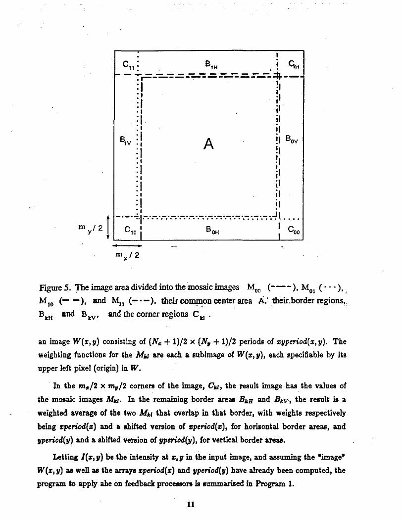
Figure 5. The image area divided into the mosaic images M00 (--- ), M01 ( • • • ), ,

M10 (- -). and M., (-·-). theirco~ncenterarea A.; _their.borderregions,,

BkH and Btv• and the comer regions Ctl .

an image W(z, y) consisting of (N., + 1)/2 x (N, + 1)/2 periods of zyperiod(z, y). The

weighting functions for ~he M~;~ are each a subimage of W(z, y), each specifiable by its

upper left pixel (origin) in W.

· In ~he m.,/2 x m,/2 corners of the image, 0~;~, the result image has ~he values of

the mosaic images M~;~. In the remaining border areas Bu and Bw, the result is a

weighted average of the two M~;~ that overlap in that border, wi~h weights respectively

being zperiod(z) and a shif~ed version of zperiod(a:), for horizontal border areas, and

yperiod(y) and a shifted version of yperiod(y), for vertical border areas.

Letting l(z, r) be the in~ensity at z, y in the inpu~ image, and assuming the •image•

W(z, y) as well as ~he arrays zperiod(z) and yperiod(y) have already been computed, the

program to apply ahe on feedback proceseors is summarized in Program 1.

11

Program 1: A he for fwlba.ck proceaaor1

/* Compute and apply mappings, histogram by histogram. * /

k=O -Fori = 1 to N,.

}}

{k = k + 1 (modulo 2); l = 0

Forj=ltoN•

{l = l + 1 (modulo 2)

Compute H = histogram(R;;)

Compute L = lookup table which is histogram equalization

mapping corresponding to H =(cumulative

histogram* output display range/ (m,.m,))

For all :~:, 11 E S;;

{Mkl(:~:, y) = L(I(:~:, y))}

I* Weight temporary images by modified bilinear weighting function, and sum results. *I Zero M(:~:, y)

For k = 0 to 1 {For l = 0 to 1

}}

/* Multiply Mkl by the appropriate part of W, and a.dd the result into M • /

{For all 2:, 11

{M(:~:,y) = M(:~:,y) +Mkl(:~:,y) • W(m,./2 + k • m .. + :~:, m,/2 +h m, + y)}

/* Fix up comers and borders. */ For k = 0 to 1 {For l = 0 to 1

{For all :~:, 11 E Ckl

}

{M(:~:,y) = M.r(:~:,y)}

}

For all :~:, 11 E B~:H

{M(:~:, y) = :~:period(m .. /2 + :~:) • M1c0(2:, y) + :~:period(3 • m .. /2 + 2:) • M~;1 (:~:, 11)}

For all :~:, J1 E B~;v

{M(:~:, 11) = yperiod(m,/2 + y) • M0~;(:~:, y) + yperiod(3 • m,/2 + y) • M1~;(:~:, y)}

12

Note that only two conaecutive rows of contextual regions are necessary to compute

m, pixel rows of the final resuU M. Each additional conaecutive row of contextual regions

suffices to complete the computation of m, additional pixel rows of the M~o~ and thus

M, as well as the computation of m, pixel rows of two additional M~o~. Thus with the

storage necessary for 2m,. pixel rows of each of the M~o~, M, and I, the ahe resuU could

be successively computed. Ther~fore, this method can apply ahe to an image N,/2 times

as large as would be needed if Program 1 were applied directly. In fact, since one could

step one contextual region at a time in the horizontal direction, as well, while handling

the second m, pixel rows of the various images, the factor by which the image size could

be increased could be even N,.N11 f(N,. + 2).

The speed of Program 1 on a feedback processor depends on whether each pixel in a

single pass through the image can contribute to or be mapped by a different mapping or

all the pixels must share the same mapping. On the latter, more conservative assumption,

N,.N, passes through the image would be required to calculate all of the histograms, and

the same number of passes would be required to apply the mappings. Four additional passes

would be necessary to compute the bilinearly weighted M~o~, and three more to sum these

results. Neglecting the time in computing the mappings from the histograms, 2N,.N11 + 7

passes would be required; for the common value for mosaic-sampled interpolative .ahe of

N,. = N11 = 8 and pass time of 1/30 sec., about 4.5 seconds would be required to apply

this algorithm. If each pixel could contribute to or be mapped by a different mapping in

a single pass through the image, the histograms could be computed in one pass and the

mappings applied in four passes (both independent of N,. and N,), for a total of 12 passes

or about 0.4 seconds.

a.2 Processor-per-Pixel Architecture

Another interesting architecture involves a small processor at each pixel and the ability

to broadcast a value to all pixels simultaneously (Austin, 1986]. With such devices the

following algorithm for uninterpolated ahe, based on computing each pixel's rank in its

contextual region, is very fast.

Let Q,., be the set of pixels u, t1 for which the pixel at (z, y) is in the contextual

region of that at (u, v). (For contextual regions that are symmetric, Q.,, is the same as

13

•

the con~~ual region aboui (s,r).) Let rank., be the rank of pixel s,r in ita contextual

region, the value to be computed.

ProgNm 1: AAt for per-piul parallel proee11or•

For s, r in ~he image

{Zero rank.,}

For s, r in ~he image

{For u,v in Q., {If i(s,y) < i(u,v)

~hen rank •• = rank •• + 1}

}

The ~otal. algorithm lakes a lime proportional to the number of pixels, if one uses .

an engine in which each pixel value l(z, r) ia broadcast in parallel to all the o~her pixels,

and ~hose in Q., which have greater intensity values have a rank counter incremented in

parallel. We presently have a design of a VLSI-baaed engine tha~ could accomplish ahe

for a 512 x 512 image in under 1 second. This engine can opera~e with a memory large

enough ~o hold only m, pixel rows of ~he image, i.e. one 11" of ~he total image.

4. QUALITY IMPROVEMENTS

4.1 Weighted Ahe

It seems unattractive for the contextual region of abe to end abruptly. If it does, one

pixel ia in the region, affecting the mapping of ~he pixel at the cen~er of ~he region, and ita

neighbor baa no effect on tha~ mapping. fUrthermore, it teems reasonable that the pixels

near the pixel whose mapping ia being calculated (the •center pixel•) ahould affect the

mapping more than those farther away. Therefore, we have created and evaluated a form

··of abe in which pixels' contribu~ion to a histogram decreases wi~h their distance from the

center pixel.

In this weighted ahe the ECR waa calculated with the area of each pixel weighted by

Nwa/W, where N ia the number of pixels in the contextual region,"'' ia the the weight the - ------

14

pixel contribute~~ to the histogram, and W is the sum of the w;. This method of calculating

the ECR proved to give a value that made ihe effect of a contextual region with a given

weighting scheme very close to that of an unweighted contextual region with the same

ECR.

Weighted ahe with a conical weighting function was ·applied to a number of CT scans

of various types, including those with sharp, strong boundaries. Little difference was

noticeable when compared to ordinary ahe with the same ECR. Because weighted ahe is

much more time consuming, we do not recommend its use.

4.2 Contrast Limitation

Ahe has produced excellent results in enhancing the signal component of an image, but

noise in the image is enhanced, too. There has been considerable debate about whether

or not enhancing noise is really a problem. Controlled tests with simple test patterns

indicate that enhancing noise proportionately with signal does not impair an observer's

ability to detect information in an image [Burgess, 1982). However, clinicians who routinely

examine images have indicated that noise enhancement is very disturbing and does cause

problems. We decided to investigate the effects of limiting contrast enhancement in cases

when the noise would otherwise become too apparent. This occurs when the range of

image intensities in a contextual region is not a good deal greater than the noise level, i.e.

in relatively homogeneous regions.

Contrast enhancement can be defined as the slope of the function mapping input

intensity to output intensity (see figure 6). We will assume that the range of input and

output intensities are the same. Then a slope of 1 involves no enhancement, and higher

slopes give increasingly higher enhancement. Thus the limitation of contrast enhancement

can be taken to involve restricting the slope of the mapping function.

With histogram equalization the mapping function m(i) is proportional to the cumu­

lative histogram [e.g Castleman, 1979):

m(i) = (Display..Range) • (Cumulative.Hiatogram(i)/ Region-Size).

Since the derivative of the cumulative histogram is the histogram, the slope of the mapping

15

,.

fundion at any input intensity, i.e. the contrast enhancement, il proportional to the height

of the hiltogram at that intensity:

dmfdi = (Dilplay.RangefRegion_Size) * hi1togram(i).

Therefore, limiting the slope of the mapping function il equivalent to clipping the height

of the histogram.

. .. _ Histogram

............ tty

Mapping function

Recorded ..... ., Aldlltrtnlled _,.,. ...

............ tty

""''"""" ..... .,

Figure 6. Contrast mapping functions and their associated original and clipped histograms.

High peaks in the hiltogram are normally caused by nearly uniform regions. In such

a case, with the mapping due to ordinary hiltogram equaliJation a narrow range of input

intensity values is mapped to a wide range of output intensity values, perhaps overenhanc­

ing the noise. But enforcing a maximum on the counts in the hiltogram will limit the

amount of contrast enhancement and thus the enhancement of noise.

16

When contrast enhancement ia reduced at one location it mut be increased in other

areas so that the entire input intensity range will be mapped to the entire output intensity

range. This corresponds to renormalizing the histogram after clipping so that its area

returns to its original value. We think of this as redistributing the clipped pixels.

We have tried two means of redistributing the clipped pixels: uniformly distribut­

ing them in all histogram bins, and distributing them into bins with contents less than

the clipping limit in proportion to their contents. The latter technique shares the intu­

itive advantage with ahe that contrast enhancement ia in proportion to need for contrast

enhancement, but it is complex and results in an undesired property: that the mapped

intensity throughout the image can be strongly changed by moving one pixel from its orig­

inal intensity to another in a bin that was formerly empty. Therefore, we have chosen the

option of uniform redistribution of clipped pixels - across the full intensity range of the

whole image. This option can be thought of as adding the contrast mapping due to the

clipped histogram to a linear mapping that achieves just the height at the maximum image

intensity such that the height of the sum is equal to the intensity range in the original

image (see figure 6).

Incorporation of histogram clipping into the existing ahe algorithm is straightforward.

One need only insert a histogram modification step into the algorithm. After each his­

togram for a contextual region is computed, it ia clipped to some value before the mapping

function is computed from it by calculating a cumulative histogram, or equivalently, ranks.

The user determines the clipping limit by specifying the limiting slope S of the inten­

sity mapping. The clipping limit C can be shown to be S times the average histogram bin

contents, since a slope of 1 corresponds to all bins having the same (average) value and

slope is proportional to the value of a histogram bin.

Adding a uniform level L to the clipped histogram will push the clipped histogram

again above the clipping limit, so the original histogram needed to be clipped at a lower

limit P such that P + L(P) is equal to the clipping ·limit (L is written as a function of P

because it depends on P)- The value of P that satisfies this equation can be found by the

binary search given in Program 3.

The resulting value of bottom is an integer, to which the remaining excess S divided by

17

Program S: Calculation of tu:tual clipping limit

Let C be the clipping limit and R the number of histogram bins in the total image

top=C

6oUom =0

while (top- bottom > 1)

{middle= (top+ bottom)/2 ·

}

S = sum over all histogram bins of the excess in that

bin over middle, if any

if S > (C- middle) * R

then top = middle

else bottom = middle

the number of bins R must be added to produce the desired P. Lis equal to the clipping -

limit minus P. Then the modified histogram value t1 in any bin is calculated from original

value tlorig by .

tl = { tlorig +. L if tlorig < P C sf tlorig ~ P

The clipped ahe technique has been applied to several different medical images, and

the results to date have been encouraging. In Figure 7 an original image and images

processed with ordinary and clipped abe, and interactive windowing are compared. Figure

8 compares interactively windowed images with those processed with clipped ahe. Note

not only the contrast in all organs simu1taneously, but also the ability to lessen the effects

of nonuniform sensitivity, as in MRI images from surface coils.

18

Figure 7. a) Original image, b) interactively windowed result, c) unclipped ahe reSult, d)

clipped ahe result with clipping limit 10, for a CT of the abdomen.

19

Figure 8. Results of clipped ahe (left) vs. results of intensity windowing (right) a) CT of

chest, b) surface coil MRI of spine, c) x-ray angiogram.

20

. ·,

6. SUMMARY

Numerous improvements to adaptive histogram equalization in speed or quality have

been auggested. AI for quality, clipped ahe has had great auccesa in both

a) showing in a single image all contrast in electronically recorded images whose range

is too wide for a nonadaptive mapping to succeed, and

b) ahowing contrast bidden in images initially recorded on film.

This method seems to have the potential of being applicable to all medical images, although

the clipping level must vary (apparently in a presettable way) with the imaging modality,

body region imaged, and imaging variables. The method has been used with considerable

auccess with light images as well.

As for speed,

a) if you have a general purpose computer, interpolative clipped ahe with mosaic sam­

pling is the method of choice, requiring a few minutes per megapixel on. common

minicomputers.

b) if you have access to a system with a feedback processor, a considerable increase in

speed can be obtained by using Program 1, with each histogram calculation followed by

the clipping step before the corresponding mapping is computed. This requires around

twenty seconds per megapixel with standard feedback processors doing arithmetic on

a full frame in 1/30 sec.

c) looking toward the future, a VLSI-based processor-per-pixel design aeems to be very

attractive, because not only can it compute ahe in a few seconds per megapixel, but

also it can do a wide range of other image processing operations fast [Austin, 1986].

ACKNOWLEDGEMENTS

We thank Paul F. G. M. van Waes, John R. Perry, Julian G. Rosenman, and Edward

V. Staab for their collaboration on clinical application of ahe. We are indebted to Joan

Savrock for manuscript preparation, to Leigh Pittman for figure preparation, and to Bo

Strain and Karen Curran for photography. This paper was prepared with the partial

eupport of NIH grants R01-CA39059 and R01-CA39060.

21

''

REFERENCES

Austin, J. D. and S. M. Pizer, "An Architecture for Fast Image Processing", Technical

Report #TR86-002, Dept. of Computer Science, University of North Carolina, 1986.

Burgess, A. E., R. F. Wagner, and R. J. Jennings, "Human Signal Detection Performance

for Noisy Medical Images," Proc. International Workshop on Physics and Engineering in

Medical Imaging, Asilomar, IEEE Computer Society, 99-105, March 10·18, 1982.

Castleman, K. R., Digital Image Processing, Englewood Cliffs, NJ: Prentice-Hall, Inc.,

1979.

Herman, G., Personal Communication, 1984.

Hummel, R. A., "Image Enhancement by Histogram Transformation", Computer Graphics

and Image Processing 6: 184-195, 1977.

Ketcham, D. J., R. W. Lowe and J. W. Weber, "Real-time Image Enhancement Tech­

niques", Seminar on Image Processing, l-6, Pacific Grove, California: Hughes Aircraft

Company, 1976.

Pizer, S.M., "Intensity Mappings for the Display of Medical Images", Functional Mapping

of Organ Systems and Other Computer Topics, Society of Nuclear Medicine, 1981.

Zimmerman, J. B., "Effectiveness of Adaptive Contrast Enhancement", Ph.D. Disserta­

tion, Department of Computer Science, University of North Carolina, 1985.

Zimmerman, J. B. and S. M. Pizer, •Evafuation of the Effectiveness of Adaptive His­

togram Equalization", Proc. £5th Fall Symposia - Imaging, November 17-22, 1985, Soc.

of Photographic Scientists and Engineers, 189-190, 1985.

22