Adaptive fuzzy systems for integrated lateral and ... · and external disturbances, the problem of...
355
Adaptive Fuzzy Systems for Integrated Lateral and Longitudinal Control of Highway Vehicles by Samaranath Ravipriya Ranatunga A thesis submitted in fulfilment of the requirements of the degree of Doctor of Philosophy in Robotics and Mechatronics Engineering of SWINBURNE UNIVERSITY OF TECHNOLOGY 2013
Transcript of Adaptive fuzzy systems for integrated lateral and ... · and external disturbances, the problem of...

Adaptive Fuzzy Systems for Integrated Lateral and Longitudinal Control of
Highway Vehicles
by
Samaranath Ravipriya Ranatunga
A thesis submitted in fulfilment of the requirements of the degree of
Doctor of Philosophy
in
Robotics and Mechatronics Engineering
of
SWINBURNE UNIVERSITY OF TECHNOLOGY
2013

ii

iii
Abstract
In this research, the problem of integrated lateral and longitudinal control of
highway vehicles is addressed using a number of adaptive fuzzy control techniques
separately. These adaptive fuzzy controllers are based on ‘Single-Model/Single-
Controller’, and several Multiple-Model/Multiple-Controller (MM/MC) models with
‘blending’ and ‘switching’ characteristics.
Firstly, a robust ‘single-adaptive fuzzy control system’ is developed in the
solution of the control problem. Another important feature of the developed controller is
to provide a basis of comparison with the ‘high-end’ MM/MC systems that are to
follow.
Having identified the highway vehicle ‘operation space’ as a ‘multiple-
environment’ due to its complicated dynamics and variations of working environments,
and external disturbances, the problem of integrated lateral and longitudinal control of
vehicles is redefined as a ‘multiple-modal’ problem. Therefore, in order to address the
control problem, MM/MC solutions are developed based on ‘blending’ and ‘switching’
of a bank of adaptive fuzzy controllers for improved control of highway vehicles.
The MM/MC models developed in this research are as follows. The first two
controller types are based on ‘blending’. These methods provide the advantage of
blending of adaptive fuzzy controllers in the bank for achieving a more prominent effect
in multiple environments. However, the third controller type is based on ‘switching’.
The resulting switching controller selects the best adaptive fuzzy controller from the
bank of controllers while isolating the rest of the controllers. These MM/MC types are
described as follows.
The first MM/MC, ‘robust multiple-adaptive fuzzy control with blending’ model
uses a fuzzy system to carryout blending of individual adaptive fuzzy controllers in the
bank to obtain a unique single control output. The blending of these adaptive fuzzy
controllers is done based on the designed fixed parameters of the fuzzy blender. The
system uses the advantage of adaptability of each fuzzy controller in the bank in
producing the final control effect.
The second MM/MC with blending category is ‘robust multiple-model PDC-based
(Parallel Distributed Compensation) multiple-adaptive fuzzy controller’, and it includes

iv
a number of ‘local’ vehicle models in each IF-THEN fuzzy rule. In addition to this,
there is a parallel set of relevant adaptive fuzzy controllers relating to each ‘local’
vehicle model in each corresponding fuzzy-rule in the controller setup.
The third controller system, a MM/MC category based on ‘switching’, is
described as follows. This controller is designed first, and then tested with simulations
by inclusion of different number of adaptive fuzzy controllers in the bank, in two
separate studies. This particular controller design can be utilized where there is a
specific need for a single controller at a time, as required by a specific scenario.
Therefore, the most suitable adaptive fuzzy controller in the bank at a time can be
selected based on the minimum value of a cost function.
All the controllers developed in this research are established with comprehensive
stability proofs based on a Lyapunov-based method, i.e. KYP (Kalman-Yakubovich-
Popov) lemma, leading to asymptotic stability at large even in the presence of extreme
conditions. In addition to that, all developed integrated lateral and longitudinal vehicle
controllers are validated using an industry-standard simulation platform, i.e.,
veDYNA® that is based on BMW 325i vehicle model of 1988, considering a number of
scenarios of external disturbance cases, e.g., un-symmetric loading of vehicle, tyre-road
friction changes and crosswind effects. In addition to that, two cases of sudden non-
catastrophic subsystem failures, e.g., a flat-tyre case and a wheel brake-cylinder defect
case, are also considered in simulations for validating the developed controllers.
Importantly, it is shown that the developed adaptive fuzzy control systems,
especially the MM/MC systems, exhibit improved results even in the presence of
external disturbances and some subsystem failures of a non-catastrophic nature.

v
Acknowledgement
I would like to thank my supervisors, Prof. Romesh Nagarajah and Dr. Zhenwei
Cao, for their unwavering support and guidance for successfully carrying out this
research study. If not for their encouragement and belief in me, this research work
would not have ended the present level.
I would also like to thank Prof. Ahmad Rad of Simon Fraser University, Canada
for providing some valuable points for improvements throughout my studies on vehicle
control.
Next, my thanks go to Cooperative Research Centre for Advanced Automotive
Technologies, (AutoCRC), Australia for supporting my PhD studies. This work would
not have been possible without the support of AutoCRC. I would like to thank all key
personnel at AutoCRC, and especially in this regard, would like to mention Ms. Kate
Neely, the former Education Manager.
My thanks also go to many personnel of supporting departments at Swinburne
University of Technology, Hawthorn campus, i.e., technical and facilities, library and IT
services. I regret the inability to mention the individuals by their name, since the list is
so large.
If not for the support of the following personnel who have extended me with some
studentships, my studies would not have been successful, especially at the initial stages.
In this regard I would like to thank Prof. Malin Premaratne of Monash University, Dr.
Yat Choy Wong, Dr. Tracy Ruan, Dr. Soulis Tavrou, Dr. Mehran Ektesabi and Mr.
Aaron Blicblou of Swinburne University of Technology.
I would also like to thank Dr. Chandana Watagodakumbura of RMIT University,
a friend, a college-mate, and a university batch-mate of mine, for encouraging and
providing some guidance for my research studies.
Finally, I would like to thank my family for being with me, with support and
encouragement, throughout the course of my study.
SRR

vi

vii
Declaration
This is to certify that:
1. This thesis contains no material which has been accepted for the award to the
candidate of any other degree or diploma, except where due reference is made in
the text of this thesis;
2. To the best of my knowledge, this thesis contains no material previously
published or written by another person except where due reference is made in
the text of this thesis; and
3. Where the work is based on joint research or publications, the relative
contributions of the respective authors are disclosed.
________________________
Samaranath Ravipriya Ranatunga (April, 2013)

viii

ix
Table of Contents
Abstract iii Acknowledgement v Declaration vii Table of Contents ix List of Figures xiii List of Tables xxv 1. Introduction............................................................................................................... 1
1.1 Research Problem and Scope of the Research ...................................................... 1
1.2 Outline of the Thesis .............................................................................................. 9
1.3 Significance of the Research and Contributions .................................................. 10
2. Literature Survey................................................................................................. .. 11
2.1 Introduction .......................................................................................................... 11
2.2 Vehicle Control .................................................................................................... 11
2.3 Adaptive Fuzzy Control Systems......................................................................... 17
2.4 Multiple-Model Control Systems......................................................................... 20
2.5 Chapter Summary ................................................................................................ 30
3. Vehicle Models in Controller Synthesis ................................................................ 31
3.1 Vehicle Model for Controller Design .................................................................. 31
3.2 VeDYNA® Vehicle Model for Controller Validation......................................... 37
3.3 Chapter Summary ................................................................................................ 53
4. Robust Single-Model Adaptive Fuzzy Control System .......................................55
4.1 Robust Single-Model Adaptive Fuzzy Control System....................................... 56
4.1.1 Introduction .............................................................................................. 56 4.1.2 Synthesis of Single-Adaptive Fuzzy Controller....................................... 56 4.1.3 Fuzzy Control: Takagi–Sugeno (T–S) Fuzzy Systems ............................ 59 4.1.4 Design of Single-Adaptive Fuzzy Controller........................................... 66 4.1.5 Training of Adaptive Fuzzy Controller Parameters ................................. 70 4.1.6 Robust Stability Analysis of Control System .......................................... 83

x
4.1.7 Simulation Studies, Results and Discussion ............................................ 89
4.2 Chapter Summary .............................................................................................. 116
5. Robust Multiple-Model Adaptive Fuzzy Control Systems – Blending (Soft-Switching) ...........................................................................................................117
5.1 Robust Multiple-Adaptive Fuzzy Control Systems with Blending ................... 118
5.1.1 Introduction............................................................................................ 118 5.1.2 Synthesis of Multiple-Adaptive Fuzzy Controller with Blending ......... 118 5.1.3 Training of Multiple-Adaptive Fuzzy Controller Parameters................ 125 5.1.4 Robust Stability Analysis of Control System ........................................ 132 5.1.5 Simulation Studies, Results and Discussion .......................................... 138
5.2 Robust Multiple-Model Fuzzy PDC-based Multiple-Adaptive Fuzzy Control System................................................................................................................ 160
5.2.1 Introduction............................................................................................ 160 5.2.2 Synthesis of Multiple-Model Fuzzy PDC-based Multiple-Adaptive Fuzzy
Controller ............................................................................................... 161 5.2.3 Robust Stability Analysis of Control System ........................................ 166 5.2.4 Implementation Design of Fuzzy PDC Control System ........................ 172 5.2.5 Simulation Studies, Results and Discussion .......................................... 189
5.3 Chapter Summary .............................................................................................. 209 6. Robust Multiple-Adaptive Fuzzy Controller – Switching (Hard-Switching).............................................................................................................................................211
6.1 Multiple-Adaptive Fuzzy Controller Systems with Switching .......................... 212 6.1.1 Introduction............................................................................................ 212
6.1.2 Synthesis of Multiple-Adaptive Fuzzy Controller with Switching........ 213 6.1.3 Robust Stability Analysis of Control System ........................................ 218 6.1.4 Simulation Studies, Results and Discussion for ‘Two’ Adaptive Fuzzy
Controllers in the Bank (Multiple-Adaptive Fuzzy Controller with Switching).............................................................................................. 226
6.1.5 Simulation Studies, Results and Discussion for ‘Four’ Adaptive Fuzzy Controllers in the Bank (Multiple-Adaptive Fuzzy Controller with Switching).............................................................................................. 246
6.2 Chapter Summary .............................................................................................. 266
7. Conclusions and Future Directions ..................................................................... 267

xi
References 271 Publications List from the Research 287 Appendix A Vehicle Model Parameters 289 Appendix B Control Structure Models in Simulink/MATLAB® 290 Appendix C Trained Parameters of Fuzzy Systems 306 Appendix D Pseudo-Codes of MATLAB® Programs Embedded in Simulink® Block
Diagrams 316

xii

xiii
List of Figures Figure No Page 3.1 Schematic diagram for the simple vehicle model............................................ 33 3.2 veDYNA® main GUI...................................................................................... 38 3.3 Accelerator pedal input.................................................................................... 38 3.4 Steering angle input ......................................................................................... 39 3.5 Brake pedal input............................................................................................. 40 3.6 Vehicle configuration setting GUI................................................................... 41 3.7 veDYNA® animation window ........................................................................ 42 3.8 veDYNA® Simulink® model setup................................................................ 42 3.9 veDYNA® Simulink® vehicle model............................................................. 43 3.10 Triggered block enclosing veDYNA® vehicle model ................................... 44 3.11 veDYNA® manoeuvre control block ............................................................. 45 3.12 Manoeuvre controller input block .................................................................. 45 3.13 Longitudinal control input .............................................................................. 46 3.14 Lateral control input ....................................................................................... 46 3.15 Control input interface to veDYNA® blocks ................................................. 47 3.16 Unsymmetrical load mass arrangement........................................................... 48 3.17 z-profile setting window ................................................................................. 49 3.18 External flat-tyre block .................................................................................... 50 3.19 External brake system block............................................................................ 51 3.20 External brake system - brake lines ................................................................. 52 4.1 Adaptive fuzzy system and PD module for longitudinal (lateral) vehicle controller ......................................................................................................................... 66 4.2 Simulink® model for data collection (input and output) (e.g. longitudinal data) ........................................................................................................................ 72 4.3 Road path profiles............................................................................................ 72 4.4 Velocity profiles of leading vehicle................................................................. 73 4.5 Longitudinal data profile for training .............................................................. 74 4.6 Lateral data profile for training........................................................................ 75 4.7 Data stream for longitudinal input data ........................................................... 76 4.8 Location of cluster centres for longitudinal data using fuzzy C-means clustering method........................................................................................................................ 76 4.9 Data stream for lateral input data..................................................................... 77 4.10 Location of cluster centres for lateral data using fuzzy C-means clustering method........................................................................................................................ 77 4.11 Longitudinal controller-ANFIS training error profile ..................................... 79 4.12 Longitudinal controller-ANFIS training: checking error profile..................... 79 4.13 Lateral controller ANFIS training error profile ............................................... 80 4.14 Lateral controller ANFIS training: checking error profile .............................. 80 4.15 Longitudinal inputs: ‘error’ fuzzy membership function ................................ 80

xiv
4.16 Longitudinal inputs: ‘error rate’ fuzzy membership function .....................81 4.17 Lateral inputs: ‘error’ fuzzy membership function......................................81 4.18 Lateral inputs: ‘error rate’ fuzzy membership function...............................81 4.19 Control surface for longitudinal adaptive fuzzy controller setup a priori....82 4.20 Control surface for lateral adaptive fuzzy controller setup a priori.............83 4.21 Road profile .................................................................................................91 4.22 Radii of curvature along the road ................................................................91 4.23 Vehicle velocities ........................................................................................92 4.24 Throttle angle: single-adaptive fuzzy vs. PD only ......................................92 4.25 Brake pedal position: single-adaptive fuzzy vs. PD only............................93 4.26 Steering angle: single-adaptive fuzzy vs. ‘PD only’ ...................................93 4.27 Lateral position of vehicle centre of gravity................................................94 4.28 Longitudinal error: single-adaptive fuzzy vs. ‘PD only’ (a) ......................95 4.29 Lateral error: single-adaptive fuzzy vs. ‘PD only’ (a) ...............................95 4.30 Pitch angle: single-adaptive fuzzy vs. ‘PD only’ (a) .................................96 4.31 Roll angle: single-adaptive fuzzy vs. ‘PD only’ (a) ..................................96 4.32 Roll rate: single-adaptive fuzzy vs. ‘PD only’ (a) .....................................96 4.33 Side-slip angle: single-adaptive fuzzy vs. ‘PD only’ (a) .............................98 4.34 Lateral acceleration: single-adaptive fuzzy vs. ‘PD only’ (a) ...................98 4.35 Longitudinal error: single-adaptive fuzzy vs. ‘PD only’ (b).1. ..................99 4.36 Lateral error: single-adaptive fuzzy vs. ‘PD only’ (b).1..............................99 4.37 Pitch angle: single-adaptive fuzzy vs. ‘PD only’ (b).1..............................100 4.38 Roll angle: single-adaptive fuzzy vs. ‘PD only’ (b).1 ...............................100 4.39 Roll rate: single-adaptive fuzzy vs. ‘PD only’ (b).1..................................100 4.40 Side-slip angle: single-adaptive fuzzy vs. ‘PD only’ (b).1 ......................101 4.41 Lateral acceleration: single-adaptive fuzzy vs. ‘PD only’ (b).1 ..............101 4.42 Longitudinal error: single-adaptive fuzzy vs. ‘PD only’ (b).2 ...............102 4.43 Lateral error: single-adaptive fuzzy vs. ‘PD only’ (b).2 ...........................102 4.44 Pitch angle: single-adaptive fuzzy vs. ‘PD only’ (b).2 .............................103 4.45 Roll angle: single-adaptive fuzzy vs. ‘PD only’ (b).2 ...............................103 4.46 Roll rate: single-adaptive fuzzy vs. ‘PD only’ (b).2..................................103 4.47 Side-slip angle: single-adaptive fuzzy vs. ‘PD only’ (b).2 .......................104 4.48 Lateral acceleration: single-adaptive fuzzy vs. ‘PD only’ (b).2................104 4.49 Longitudinal error: single-adaptive fuzzy vs. ‘PD only’ (b).3 .................105 4.50 Lateral error: single-adaptive fuzzy vs. ‘PD only’ (b).3 ...........................105 4.51 Pitch angle: single-adaptive fuzzy vs. ‘PD only’ (b).3..............................105 4.52 Roll angle: single-adaptive fuzzy vs. ‘PD only’ (b).3 ..............................106 4.53 Roll rate: single-adaptive fuzzy vs. ‘PD only’ (b).3 .................................106 4.54 Side-slip angle: single-adaptive fuzzy vs. ‘PD only’ (b).3 .......................106 4.55 Lateral acceleration: single-adaptive fuzzy vs. ‘PD only’ (b).3 ...............107 4.56 Longitudinal error: single-adaptive fuzzy vs. ‘PD only’ (c).1 .................108 4.57 Lateral error: single-adaptive fuzzy vs. ‘PD only’ (c).1 ..........................108 4.58 Pitch angle: single-adaptive fuzzy vs. ‘PD only’ (c).1..............................109 4.59 Roll angle: single-adaptive fuzzy vs. ‘PD only’ (c).1 ...............................109 4.60 Roll rate: single-adaptive fuzzy vs. ‘PD only’ (c).1..................................110 4.61 Side-slip angle: single-adaptive fuzzy vs. ‘PD only’ (c).1........................110

xv
4.62 Lateral acceleration: single-adaptive fuzzy vs. ‘PD only’ (c).1 ...............111 4.63 Longitudinal error: single-adaptive fuzzy vs. ‘PD only’ (c).2 .................112 4.64 Lateral error: single-adaptive fuzzy vs. ‘PD only’ (c).2 ..........................112 4.65 Pitch angle: single-adaptive fuzzy vs. ‘PD only’ (c).2 ............................112 4.66 Roll angle: single-adaptive fuzzy vs. ‘PD only’ (c).2 .............................113 4.67 Roll rate: single-adaptive fuzzy vs. ‘PD only’ (c).2 ................................113 4.68 Side-slip angle: single-adaptive fuzzy vs. ‘PD only’ (c).2 ......................113 4.69 Lateral acceleration: single-adaptive fuzzy vs. ‘PD only’ (c).2 ..............114 5.1 Schematic diagram of multiple-adaptive fuzzy controller with fuzzy blender for longitudinal (lateral) control ................................................................................120 5.2 Train data (inputs) for ANFIS training of longitudinal fuzzy blender .....128 5.3 Train data (output) for ANFIS training of longitudinal fuzzy blender .....128 5.4 Training error for ANFIS training of longitudinal fuzzy blender .............128 5.5 Checking error for validation of ANFIS training of longitudinal fuzzy blender ...................................................................................................................129 5.6 Control surface for longitudinal fuzzy blender .........................................129 5.7 Train data (inputs) for ANFIS training of lateral fuzzy blender ...............130 5.8 Train data (output) for ANFIS training of lateral fuzzy blender ..............130 5.9 Training error for ANFIS training of lateral fuzzy blender ......................130 5.10 Checking error for validation of ANFIS training of lateral fuzzy blender 131 5.11 Control surface for lateral fuzzy blender ...................................................131 5.12 Longitudinal error: multiple-adaptive fuzzy with blending vs. single-adaptive fuzzy (a) .............................................................................................................139 5.13 Lateral error: multiple-adaptive fuzzy with blending vs. single-adaptive fuzzy (a) ...................................................................................................................139 5.14 Pitch angle: multiple-adaptive fuzzy with blending vs. single-adaptive fuzzy (a) ...................................................................................................................140 5.15 Roll angle: multiple-adaptive fuzzy with blending vs. single-adaptive fuzzy (a) ...................................................................................................................140 5.16 Roll rate: multiple-adaptive fuzzy with blending vs. single-adaptive fuzzy (a) ...................................................................................................................140 5.17 Side-slip angle: multiple-adaptive fuzzy with blending vs. single-adaptive fuzzy (a) ..................................................................................................................141 5.18 Lateral acceleration: multiple-adaptive fuzzy with blending vs. single-adaptive fuzzy (a) ...............................................................................................................141 5.19 Longitudinal error: multiple-adaptive fuzzy with blending vs. single-adaptive fuzzy (b).1 ............................................................................................................143 5.20 Lateral error: multiple-adaptive fuzzy with blending vs. single-adaptive fuzzy (b).1 ...................................................................................................................143 5.21 Pitch angle: multiple-adaptive fuzzy with blending vs. single-adaptive fuzzy (b).1 ...................................................................................................................143 5.22 Roll angle: multiple-adaptive fuzzy with blending vs. single-adaptive fuzzy (b).1 ...................................................................................................................144 5.23 Roll rate: multiple-adaptive fuzzy with blending vs. single-adaptive fuzzy (b).1 ...................................................................................................................144

xvi
5.24 Side-slip angle: multiple-adaptive fuzzy with blending vs. single-adaptive fuzzy (b).1 ...................................................................................................................144 5.25 Lateral acceleration: multiple-adaptive fuzzy with blending vs. single-adaptive fuzzy (b).1 ............................................................................................................145 5.26 Longitudinal error: multiple-adaptive fuzzy with blending vs. single-adaptive fuzzy (b).2 ............................................................................................................146 5.27 Lateral error: multiple-adaptive fuzzy with blending vs. single-adaptive fuzzy (b).2 ...................................................................................................................146 5.28 Pitch angle: multiple-adaptive fuzzy with blending vs. single-adaptive fuzzy (b).2 ...................................................................................................................147 5.29 Roll angle: multiple-adaptive fuzzy with blending vs. single-adaptive fuzzy (b).2 ...................................................................................................................147 5.30 Roll rate: multiple-adaptive fuzzy with blending vs. single-adaptive fuzzy (b).2 ...................................................................................................................147 5.31 Side-slip angle: multiple-adaptive fuzzy with blending vs. single-adaptive fuzzy (b).2 ...................................................................................................................148 5.32 Lateral acceleration: multiple-adaptive fuzzy with blending vs. single-adaptive fuzzy (b).2 ............................................................................................................149 5.33 Longitudinal error: multiple-adaptive fuzzy with blending vs. single-adaptive fuzzy (b).3 ............................................................................................................149 5.34 Lateral error: multiple-adaptive fuzzy with blending vs. single-adaptive fuzzy (b).3 ...................................................................................................................150 5.35 Pitch angle: multiple-adaptive fuzzy with blending vs. single-adaptive fuzzy (b).3 ...................................................................................................................150 5.36 Roll angle: multiple-adaptive fuzzy with blending vs. single-adaptive fuzzy (b).3 ...................................................................................................................150 5.37 Roll rate: multiple-adaptive fuzzy with blending vs. single-adaptive fuzzy (b).3 ...................................................................................................................151 5.38 Side-slip angle: multiple-adaptive fuzzy with blending vs. single-adaptive fuzzy (b).3 ...................................................................................................................151 5.39 Lateral acceleration: multiple-adaptive fuzzy with blending vs. single-adaptive fuzzy (b).3 ............................................................................................................152 5.40 Longitudinal error: multiple-adaptive fuzzy with blending vs. single-adaptive fuzzy (c).1 ............................................................................................................153 5.41 Lateral error: multiple-adaptive fuzzy with blending vs. single-adaptive fuzzy (c).1 ...................................................................................................................153 5.42 Pitch angle: multiple-adaptive fuzzy with blending vs. single-adaptive fuzzy (c).1 ...................................................................................................................153 5.43 Roll angle: multiple-adaptive fuzzy with blending vs. single-adaptive fuzzy (c).1 ...................................................................................................................154 5.44 Roll rate: multiple-adaptive fuzzy with blending vs. single-adaptive fuzzy (c).1 ...................................................................................................................154 5.45 Side-slip angle: multiple-adaptive fuzzy with blending vs. single-adaptive fuzzy (c).1 ...................................................................................................................154 5.46 Lateral acceleration: multiple-adaptive fuzzy with blending vs. single-adaptive fuzzy (c).1 ............................................................................................................155

xvii
5.47 Longitudinal error: multiple-adaptive fuzzy with blending vs. single-adaptive fuzzy (c).2 ...........................................................................................................156 5.48 Lateral error: multiple-adaptive fuzzy with blending vs. single-adaptive fuzzy (c).2 ...................................................................................................................156 5.49 Pitch angle: multiple-adaptive fuzzy with blending vs. single-adaptive fuzzy (c).2 ...................................................................................................................156 5.50 Roll angle: multiple-adaptive fuzzy with blending vs. single-adaptive fuzzy (c).2 ...................................................................................................................157 5.51 Roll rate: multiple-adaptive fuzzy with blending vs. single-adaptive fuzzy (c).2 ...................................................................................................................157 5.52 Side-slip angle: multiple-adaptive fuzzy with blending vs. single-adaptive fuzzy (c).2 ...................................................................................................................158 5.53 Lateral acceleration: multiple-adaptive fuzzy with blending vs. single-adaptive fuzzy (c).2 .........................................................................................................158 5.54 Schematic diagram for fuzzy Parallel Distributed Compensation (PDC) scheme ...................................................................................................................163 5.55 Fuzzy input membership functions............................................................179 5.56 Adaptive fuzzy longitudinal controller output surfaces.............................185 5.57 Adaptive fuzzy lateral controller output surfaces......................................186 5.58 Longitudinal controller training and validation errors...............................187 5.59 Lateral controller training and validation errors........................................188 5.60 Longitudinal error: PDC-based multiple-adaptive fuzzy with blending vs. single-adaptive fuzzy (a).................................................................................................190 5.61 Lateral error: PDC-based multiple-adaptive fuzzy with blending vs. single-adaptive fuzzy (a).................................................................................................190 5.62 Pitch angle: PDC-based multiple-adaptive fuzzy with blending vs. single-adaptive fuzzy (a).................................................................................................190 5.63 Roll angle: PDC-based multiple-adaptive fuzzy with blending vs. single-adaptive fuzzy (a) ...............................................................................................................191 5.64 Roll rate: PDC-based multiple-adaptive fuzzy with blending vs. single-adaptive fuzzy (a) ...............................................................................................................191 5.65 Side-slip angle: PDC-based multiple-adaptive fuzzy with blending vs. single-adaptive fuzzy (a).................................................................................................191 5.66 Lateral acceleration: PDC-based multiple-adaptive fuzzy with blending vs. single-adaptive fuzzy (a) ......................................................................................192 5.67 Longitudinal error: PDC-based multiple-adaptive fuzzy with blending vs. single-adaptive fuzzy (b).1...................................................................................193 5.68 Lateral error: PDC-based multiple-adaptive fuzzy with blending vs. single-adaptive fuzzy (b).1..............................................................................................193 5.69 Pitch angle: PDC-based multiple-adaptive fuzzy with blending vs. single-adaptive fuzzy (b).1..............................................................................................194 5.70 Roll angle: PDC-based multiple-adaptive fuzzy with blending vs. single-adaptive fuzzy (b).1 ...........................................................................................................194 5.71 Roll rate: PDC-based multiple-adaptive fuzzy with blending vs. single-adaptive fuzzy (b).1 ............................................................................................................194

xviii
5.72 Side-slip angle: PDC-based multiple-adaptive fuzzy with blending vs. single-adaptive fuzzy (b).1..............................................................................................195 5.73 Lateral acceleration: PDC-based multiple-adaptive fuzzy with blending vs. single-adaptive fuzzy (b).1.................................................................................. 195 5.74 Longitudinal error: PDC-based multiple-adaptive fuzzy with blending vs. single-adaptive fuzzy (b).2..............................................................................................196 5.75 Lateral error: PDC-based multiple-adaptive fuzzy with blending vs. single-adaptive fuzzy (b).2..............................................................................................196 5.76 Pitch angle: PDC-based multiple-adaptive fuzzy with blending vs. single-adaptive fuzzy (b).2 .............................................................................................197 5.77 Roll angle: PDC-based multiple-adaptive fuzzy with blending vs. single-adaptive fuzzy (b).2 ............................................................................................................197 5.78 Roll rate: PDC-based multiple-adaptive fuzzy with blending vs. single-adaptive fuzzy (b).2 ............................................................................................................197 5.79 Side-slip angle: PDC-based multiple-adaptive fuzzy with blending vs. single-adaptive fuzzy (b).2..............................................................................................198 5.80 Lateral acceleration: PDC-based multiple-adaptive fuzzy with blending vs. single-adaptive fuzzy (b).2...................................................................................198 5.81 Longitudinal error: PDC-based multiple-adaptive fuzzy with blending vs. single-adaptive fuzzy (b).3..............................................................................................199 5.82 Lateral error: PDC-based multiple-adaptive fuzzy with blending vs. single-adaptive fuzzy (b).3..............................................................................................199 5.83 Pitch angle: PDC-based multiple-adaptive fuzzy with blending vs. single-adaptive fuzzy (b).3..............................................................................................199 5.84 Roll angle: PDC-based multiple-adaptive fuzzy with blending vs. single-adaptive fuzzy (b).3 ............................................................................................................200 5.85 Roll rate: PDC-based multiple-adaptive fuzzy with blending vs. single-adaptive fuzzy (b).3 ............................................................................................................200 5.86 Side-slip angle: PDC-based multiple-adaptive fuzzy with blending vs. single-adaptive fuzzy (b).3 .............................................................................................200 5.87 Lateral acceleration: PDC-based multiple-adaptive fuzzy with blending vs. single-adaptive fuzzy (b).3 ..................................................................................201 5.88 Longitudinal error: PDC-based multiple-adaptive fuzzy with blending vs. single-adaptive fuzzy (c).1..............................................................................................202 5.89 Lateral error: PDC-based multiple-adaptive fuzzy with blending vs. single-adaptive fuzzy (c).1..............................................................................................202 5.90 Pitch angle: PDC-based multiple-adaptive fuzzy with blending vs. single-adaptive fuzzy (c).1..............................................................................................203 5.91 Roll angle: PDC-based multiple-adaptive fuzzy with blending vs. single-adaptive fuzzy (c).1 ............................................................................................................203 5.92 Roll rate: PDC-based multiple-adaptive fuzzy with blending vs. single-adaptive fuzzy (c).1 ...........................................................................................................203 5.93 Side-slip angle: PDC-based multiple-adaptive fuzzy with blending vs. single-adaptive fuzzy (c).1..............................................................................................204 5.94 Lateral acceleration: PDC-based multiple-adaptive fuzzy with blending vs. single-adaptive fuzzy (c).1...................................................................................204

xix
5.95 Longitudinal error: PDC-based multiple-adaptive fuzzy with blending vs. single-adaptive fuzzy (c).2 ...........................................................................................205 5.96 Lateral error: PDC-based multiple-adaptive fuzzy with blending vs. single-adaptive fuzzy (c).2 ............................................................................................205 5.97 Pitch angle: PDC-based multiple-adaptive fuzzy with blending vs. single-adaptive fuzzy (c).2 ............................................................................................205 5.98 Roll angle: PDC-based multiple-adaptive fuzzy with blending vs. single-adaptive fuzzy (c).2 ..........................................................................................................206 5.99 Roll rate: PDC-based multiple-adaptive fuzzy with blending vs. single-adaptive fuzzy (c).2 ..........................................................................................................206 5.100 Side-slip angle: PDC-based multiple-adaptive fuzzy with blending vs. single-adaptive fuzzy (c).2 ...........................................................................................207 5.101 Lateral acceleration: PDC-based multiple-adaptive fuzzy with blending vs. single-adaptive fuzzy (c).2 .................................................................................207 6.1 Schematics of multiple-adaptive fuzzy controller system with switching (state showing nth adaptive fuzzy controller switched on) consisting n adaptive fuzzy controllers in the bank..........................................................................................214 6.2 Longitudinal error: multiple-adaptive fuzzy with switching (2-AFCs in the bank) vs. single-adaptive fuzzy (a) ................................................................................227 6.3 Lateral error: multiple-adaptive fuzzy with switching (2-AFCs in the bank) vs. single-adaptive fuzzy (a) ......................................................................................227 6.4 Pitch angle: multiple-adaptive fuzzy with switching (2-AFCs in the bank) vs. single-adaptive fuzzy (a) ......................................................................................228 6.5 Roll angle: multiple-adaptive fuzzy with switching (2-AFCs in the bank) vs. single-adaptive fuzzy (a) ......................................................................................228 6.6 Roll rate: multiple-adaptive fuzzy with switching (2-AFCs in the bank) vs. single-adaptive fuzzy (a) ...............................................................................................228 6.7 Side-slip angle: multiple-adaptive fuzzy with switching (2-AFCs in the bank) vs. single-adaptive fuzzy (a) ......................................................................................229 6.8 Lateral acceleration: multiple-adaptive fuzzy with switching (2-AFCs in the bank) vs. single-adaptive fuzzy (a) ......................................................................229 6.9 Longitudinal error: multiple-adaptive fuzzy with switching (2-AFCs in the bank) vs. single-adaptive fuzzy (b).1 .............................................................................230 6.10 Lateral error: multiple-adaptive fuzzy with switching (2-AFCs in the bank) vs. single-adaptive fuzzy (b).1...................................................................................230 6.11 Pitch angle: multiple-adaptive fuzzy with switching (2-AFCs in the bank) vs. single-adaptive fuzzy (b).1...................................................................................231 6.12 Roll angle: multiple-adaptive fuzzy with switching (2-AFCs in the bank) vs. single-adaptive fuzzy (b).1...................................................................................231 6.13 Roll rate: multiple-adaptive fuzzy with switching (2-AFCs in the bank) vs. single-adaptive fuzzy (b).1 .............................................................................................231 6.14 Side slip angle: multiple-adaptive fuzzy with switching (2-AFCs in the bank) vs. single-adaptive fuzzy (b).1...................................................................................232 6.15 Lateral acceleration: multiple-adaptive fuzzy with switching (2-AFCs in the bank) vs. single-adaptive fuzzy (b).1 ...................................................................232
xx
6.16 Longitudinal error: multiple-adaptive fuzzy with switching (2-AFCs in the bank) vs. single-adaptive fuzzy (b).2 .............................................................................233 6.17 Lateral error: multiple-adaptive fuzzy with switching (2-AFCs in the bank) vs. single-adaptive fuzzy (b).2.................................................................................. 233 6.18 Pitch angle: multiple-adaptive fuzzy with switching (2-AFCs in the bank) vs. single-adaptive fuzzy (b).2...................................................................................233 6.19 Roll angle: multiple-adaptive fuzzy with switching (2-AFCs in the bank) vs. single-adaptive fuzzy (b).2...................................................................................234 6.20 Roll rate: multiple-adaptive fuzzy with switching (2-AFCs in the bank) vs. single-adaptive fuzzy (b).2 .............................................................................................234 6.21 Side-slip angle: multiple-adaptive fuzzy with switching (2-AFCs in the bank) vs. single-adaptive fuzzy (b).2...................................................................................234 6.22 Lateral acceleration: multiple-adaptive fuzzy with switching (2-AFCs in the bank) vs. single-adaptive fuzzy (b).2...................................................................235 6.23 Longitudinal error: multiple-adaptive fuzzy with switching (2-AFCs in the bank) vs. single-adaptive fuzzy (b).3 .............................................................................236 6.24 Lateral error: multiple-adaptive fuzzy with switching (2-AFCs in the bank) vs. single-adaptive fuzzy (b).3...................................................................................236 6.25 Pitch angle: multiple-adaptive fuzzy with switching (2-AFCs in the bank) vs. single-adaptive fuzzy (b).3...................................................................................236 6.26 Roll angle: multiple-adaptive fuzzy with switching (2-AFCs in the bank) vs. single-adaptive fuzzy (b).3...................................................................................237 6.27 Roll rate: multiple-adaptive fuzzy with switching (2-AFCs in the bank) vs. single-adaptive fuzzy (b).3..............................................................................................237 6.28 Side-slip angle: multiple-adaptive fuzzy with switching (2-AFCs in the bank) vs. single-adaptive fuzzy (b).3...................................................................................237 6.29 Lateral acceleration: multiple-adaptive fuzzy with switching (2-AFCs in the bank) vs. single-adaptive fuzzy (b).3...................................................................238 6.30 Longitudinal error: multiple-adaptive fuzzy with switching (2-AFCs in the bank) vs. single-adaptive fuzzy (c).1 .............................................................................239 6.31 Lateral error: multiple-adaptive fuzzy with switching (2-AFCs in the bank) vs. single-adaptive fuzzy (c).1...................................................................................239 6.32 Pitch angle: multiple-adaptive fuzzy with switching (2-AFCs in the bank) vs. single-adaptive fuzzy (c).1...................................................................................239 6.33 Roll angle: multiple-adaptive fuzzy with switching (2-AFCs in the bank) vs. single-adaptive fuzzy (c).1...................................................................................240 6.34 Roll rate: multiple-adaptive fuzzy with switching (2-AFCs in the bank) vs. single-adaptive fuzzy (c).1 .............................................................................................240 6.35 Side-slip angle: multiple-adaptive fuzzy with switching (2-AFCs in the bank) vs. single-adaptive fuzzy (c).1...................................................................................240 6.36 Lateral acceleration: multiple-adaptive fuzzy with switching (2-AFCs in the bank) vs. single-adaptive fuzzy (c).1 ...................................................................241 6. 37 Longitudinal error: multiple-adaptive fuzzy with switching (2-AFCs in the bank) vs. single-adaptive fuzzy (c).2 ...........................................................................242 6.38 Lateral error: multiple-adaptive fuzzy with switching (2-AFCs in the bank) vs. single-adaptive fuzzy (c).2 .................................................................................242

xxi
6.39 Pitch angle: multiple-adaptive fuzzy with switching (2-AFCs in the bank) vs. single-adaptive fuzzy (c).2 .................................................................................242 6.40 Roll angle: multiple-adaptive fuzzy with switching (2-AFCs in the bank) vs. single-adaptive fuzzy (c).2 .................................................................................243 6.41 Roll rate: multiple-adaptive fuzzy with switching (2-AFCs in the bank) vs. single-adaptive fuzzy (c).2 ...........................................................................................243 6.42 Side-slip angle: multiple-adaptive fuzzy with switching (2-AFCs in the bank) vs. single-adaptive fuzzy (c).2 .................................................................................243 6.43 Lateral acceleration: multiple-adaptive fuzzy with switching (2-AFCs in the bank) vs. single-adaptive fuzzy (c).2 .................................................................244 6.44 Longitudinal error: multiple-adaptive fuzzy with switching (4-AFCs in the bank) vs. single-adaptive fuzzy (a) ................................................................................247 6.45 Lateral error: multiple-adaptive fuzzy with switching (4-AFCs in the bank) vs. single-adaptive fuzzy (a) ......................................................................................247 6.46 Pitch angle: multiple-adaptive fuzzy with switching (4-AFCs in the bank) vs. single-adaptive fuzzy (a) ......................................................................................247 6.47 Roll angle: multiple-adaptive fuzzy with switching (4-AFCs in the bank) vs. single-adaptive fuzzy (a) ......................................................................................248 6.48 Roll rate: multiple-adaptive fuzzy with switching (4-AFCs in the bank) vs. single-adaptive fuzzy (a) ...............................................................................................248 6.49 Side-slip angle: multiple-adaptive fuzzy with switching (4-AFCs in the bank) vs. single-adaptive fuzzy (a) ......................................................................................248 6.50 Lateral acceleration: multiple-adaptive fuzzy with switching (4-AFCs in the bank) vs. single-adaptive fuzzy (a) ......................................................................249 6.51 Longitudinal error: multiple-adaptive fuzzy with switching (4-AFCs in the bank) vs. single-adaptive fuzzy (b).1 .............................................................................250 6.52 Lateral error: multiple-adaptive fuzzy with switching (4-AFCs in the bank) vs. single-adaptive fuzzy (b).1...................................................................................250 6.53 Pitch angle: multiple-adaptive fuzzy with switching (4-AFCs in the bank) vs. single-adaptive fuzzy (b).1...................................................................................251 6.54 Roll angle: multiple-adaptive fuzzy with switching (4-AFCs in the bank) vs. single-adaptive fuzzy (b).1...................................................................................251 6.55 Roll rate: multiple-adaptive fuzzy with switching (4-AFCs in the bank) vs. single-adaptive fuzzy (b).1 .............................................................................................251 6.56 Side-slip angle: multiple-adaptive fuzzy with switching (4-AFCs in the bank) vs. single-adaptive fuzzy (b).1...................................................................................252 6.57 Lateral acceleration: multiple-adaptive fuzzy with switching (4-AFCs in the bank) vs. single-adaptive fuzzy (b).1 ...................................................................252 6.58 Longitudinal error: multiple-adaptive fuzzy with switching (4-AFCs in the bank) vs. single-adaptive fuzzy (b).2 .............................................................................253 6.59 Lateral error: multiple-adaptive fuzzy with switching (4-AFCs in the bank) vs. single-adaptive fuzzy (b).2...................................................................................253 6.60 Pitch angle: multiple-adaptive fuzzy with switching (4-AFCs in the bank) vs. single-adaptive fuzzy (b).2...................................................................................254 6.61 Roll angle: multiple-adaptive fuzzy with switching (4-AFCs in the bank) vs. single-adaptive fuzzy (b).2...................................................................................254
xxii
6.62 Roll rate: multiple-adaptive fuzzy with switching (4-AFCs in the bank) vs. single-adaptive fuzzy (b).2..............................................................................................254 6.63 Side-slip angle: multiple-adaptive fuzzy with switching (4-AFCs in the bank) vs. single-adaptive fuzzy (b).2................................................................................. 255 6.64 Lateral acceleration: multiple-adaptive fuzzy with switching (4-AFCs in the bank) vs. single-adaptive fuzzy (b).2...................................................................255 6.65 Longitudinal error: multiple-adaptive fuzzy with switching (4-AFCs in the bank) vs. single-adaptive fuzzy (b).3 .............................................................................256 6.66 Lateral error: multiple-adaptive fuzzy with switching (4-AFCs in the bank) vs. single-adaptive fuzzy (b).3...................................................................................256 6.67 Pitch angle: multiple-adaptive fuzzy with switching (4-AFCs in the bank) vs. single-adaptive fuzzy (b).3...................................................................................256 6.68 Roll angle: multiple-adaptive fuzzy with switching (4-AFCs in the bank) vs. single-adaptive fuzzy (b).3...................................................................................257 6.69 Roll rate: multiple-adaptive fuzzy with switching (4-AFCs in the bank) vs. single-adaptive fuzzy (b).3..............................................................................................257 6.70 Side-slip angle: multiple-adaptive fuzzy with switching (4-AFCs in the bank) vs. single-adaptive fuzzy (b).3...................................................................................257 6.71 Lateral acceleration: multiple-adaptive fuzzy with switching (4-AFCs in the bank) vs. single-adaptive fuzzy (b).3...................................................................258 6.72 Longitudinal error: multiple-adaptive fuzzy with switching (4-AFCs in the bank) vs. single-adaptive fuzzy (c).1 .............................................................................259 6.73 Lateral error: multiple-adaptive fuzzy with switching (4-AFCs in the bank) vs. single-adaptive fuzzy (c).1...................................................................................259 6.74 Pitch angle: multiple-adaptive fuzzy with switching (4-AFCs in the bank) vs. single-adaptive fuzzy (c).1...................................................................................259 6.75 Roll angle: multiple-adaptive fuzzy with switching (4-AFCs in the bank) vs. single-adaptive fuzzy (c).1...................................................................................260 6.76 Roll rate: multiple-adaptive fuzzy with switching (4-AFCs in the bank) vs. single-adaptive fuzzy (c).1..............................................................................................260 6.77 Side-slip angle: multiple-adaptive fuzzy with switching (4-AFCs in the bank) vs. single-adaptive fuzzy (c).1...................................................................................260 6.78 Lateral acceleration: multiple-adaptive fuzzy with switching (4-AFCs in the bank) vs. single-adaptive fuzzy (c).1 ...................................................................261 6.79 Longitudinal error: multiple-adaptive fuzzy with switching (4-AFCs in the bank) vs. single-adaptive fuzzy (c).2 .............................................................................262 6.80 Lateral error: multiple-adaptive fuzzy with switching (4-AFCs in the bank) vs. single-adaptive fuzzy (c).2...................................................................................262 6.81 Pitch angle: multiple-adaptive fuzzy with switching (4-AFCs in the bank) vs. single-adaptive fuzzy (c).2...................................................................................262 6.82 Roll angle: multiple-adaptive fuzzy with switching (4-AFCs in the bank) vs. single-adaptive fuzzy (c).2...................................................................................263 6.83 Roll rate: multiple-adaptive fuzzy with switching (4-AFCs in the bank) vs. single-adaptive fuzzy (c).2..............................................................................................263 6.84 Side-slip angle: multiple-adaptive fuzzy with switching (4-AFCs in the bank) vs. single-adaptive fuzzy (c).2...................................................................................263

xxiii
6.85 Lateral acceleration: multiple-adaptive fuzzy with switching (4-AFCs in the bank) vs. single-adaptive fuzzy (c).2 ...................................................................264 B.1 Main control block (Single-model adaptive fuzzy controller) ..................290 B.2 Lateral error calculation (Single-model adaptive fuzzy controller) ..........290 B.3 Variable structure control (Single-model adaptive fuzzy controller) ........290 B.4 Inverse model for vehicle control input calculation (Single-model adaptive fuzzy controller).............................................................................................................291 B.5 Calculation of combined longitudinal and steering inputs (Single-model adaptive fuzzy controller) ...................................................................................................291 B.6 Calculation of engine speed (Single-model adaptive fuzzy controller).....291 B.7 Calculation of combined longitudinal inputs (Single-model adaptive fuzzy controller).............................................................................................................292 B.8 Calculation of front slip angles (Single-model adaptive fuzzy controller)292 B.9 Calculation of states of vehicle for slip angle calculation (Single-model adaptive fuzzy controller) ...................................................................................................292 B.10 Vehicle model calculations for control inputs (Single-model adaptive fuzzy controller).............................................................................................................293 B.11 Longitudinal model calculations (Single-model adaptive fuzzy controller) ... ...................................................................................................................293 B.12 Lateral model calculations (Single-model adaptive fuzzy controller).......294 B.13 Adaptive fuzzy controller-longitudinal (Single-model adaptive fuzzy controller) ...................................................................................................................294 B.14 Adaptive fuzzy controller-lateral (Single-model adaptive fuzzy controller)... ...................................................................................................................294 B.15 Main control block (Multiple-adaptive fuzzy controller) ..........................295 B.16 Lateral control block (Multiple-adaptive fuzzy controller) .......................295 B.17 Longitudinal control block (Multiple-adaptive fuzzy controller)..............296 B.18 Fuzzy blender- lateral (Multiple-adaptive fuzzy controller) .....................296 B.19 Fuzzy blender-longitudinal (Multiple-adaptive fuzzy controller) .............296 B.20 Main control block (Multiple-model PDC controller)...............................297 B.21 Longitudinal control block (Multiple-model PDC controller) ..................297 B.22 Control inputs for fuzzy blending – longitudinal (Multiple-model PDC controller) ...................................................................................................................298 B.23 Vehicle local models – longitudinal (Multiple-model PDC controller) ....298 B.24 Lateral control block (Multiple-model PDC controller)............................299 B.25 Control inputs for fuzzy blending – lateral (Multiple-model PDC controller) ...................................................................................................................299 B.26 Vehicle local models – lateral (Multiple-model PDC controller) .............300 B.27 Main control block (Multiple-adaptive fuzzy control with switching: 2-AFCs) ...................................................................................................................300 B.28 Multiple-adaptive fuzzy control with switching – lateral (Multiple-adaptive fuzzy control with switching: 2-AFCs)..........................................................................301 B.29 Multiple-adaptive fuzzy control with switching – longitudinal (Multiple-adaptive fuzzy control with switching: 2-AFCs)................................................................301
xxiv
B.30 Cost function comparator for switching (lateral/longitudinal) (Multiple-adaptive fuzzy control with switching: 2-AFCs)................................................................302 B.31 Controller switcher (longitudinal/ lateral) (Multiple-adaptive fuzzy control with switching: 2-AFCs)..............................................................................................302 B.32 Cost function for controller switching (w1 and w2) (Multiple-adaptive fuzzy control with switching: 2-AFCs)..........................................................................302 B.33 Main control block (Multiple-adaptive fuzzy control with switching: 4-AFCs) ...................................................................................................................303 B.34 Multiple-adaptive fuzzy control with switching – longitudinal (Multiple-adaptive fuzzy control with switching: 4-AFCs)................................................................303 B.35 Cost function comparator for switching – longitudinal (Multiple-adaptive fuzzy control with switching: 4-AFCs)..........................................................................304 B.36 Controller switcher – longitudinal (Multiple-adaptive fuzzy control with switching: 4-AFCs)..............................................................................................304 B.37 Multiple-adaptive fuzzy control with switching – lateral (Multiple-adaptive fuzzy control with switching: 4-AFCs)..........................................................................305 B.38 Cost function comparator for switching – lateral (Multiple-adaptive fuzzy control with switching: 4-AFCs)......................................................................................305 B.39 Controller switcher – lateral (Multiple-adaptive fuzzy control with switching: 4-AFCs)...................................................................................................................305

xxv
List of Tables Table No Page 4.1 Comparison of performance of single-adaptive fuzzy controller against ‘PD only’ controller ....................................................................................................................115 5.1 Comparison of performance of multiple-adaptive fuzzy controller against single-adaptive fuzzy controller............................................................................................ 159 5.2 Comparison of performance of fuzzy PDC based multiple-adaptive fuzzy controller against single-adaptive fuzzy controller.................................................... 208 6.1 Comparison of performance of fuzzy multiple-adaptive fuzzy controller (2-AFCs) against single-adaptive fuzzy controller..................................................................... 245 6.2 Comparison of performance of fuzzy multiple-adaptive fuzzy controller (4-AFCs) against single-adaptive fuzzy controller..................................................................... 265


1
C H A P T E R 1
Introduction Full automation of highway vehicles has almost been achieved in the present day due to
developments in microprocessors, advanced sensor technologies, and communication
technologies. An unceasing trend is underway for further development of ‘smart’ or
‘intelligent’ vehicles towards fully-fledged automation that will result in improved
passenger safety while making the road more efficient with improved traffic flow, to
name a few advantages.
1.1 Research Problem and Scope of the Research
1.1.1 Automation of Highway Vehicles for Safety and Higher Road
Throughput
Intelligent vehicle controller designs can realize improved safety for passengers
by way of precision operation and manoeuvring of automated vehicular systems — an
answer to the problem that significant proportion of highway fatalities are due to human
error [1]. The large number of road accidents due to human error validated facts given
by the World Health Organization, which has identified road accidents as the ninth
leading cause of death throughout the world in 2004 [2]. It is an important fact that the
attention of drivers is not fully dedicated to driving task all the time. Such diversion of
attention from driving can no doubt have serious consequences for safety [3]. In
addition to that, the nature of humans is to panic in an emergency situation. This nature
of humans further distances the proper and safe decision making at such a critical time.
Apart from that fact, it takes a certain amount of time for processing decisions in
humans, i.e., feeding signals to the brain (time for sensor stimuli to reach brain), for

2
correct identification of the scenario in its correct perspective, the decision for action
and then activating it through hands/limbs (travel times of impulses to muscles) [4], for
performing driving related tasks, e.g. turning of steering wheel/pressing of brake pedals.
This time can be on the higher side at a critical point in the decision making, for
example during collision prevention, or during other emergency manoeuvres on the
road. Therefore, for overcoming ‘human error’ in handling vehicles, automating the
control of highway vehicles is an effective solution since the advanced communication
and processing technologies reduce the time factors dramatically improving safety.
The other main advantage of automation is to improve the throughput or the
number of vehicles that can use the road at a specific period of time. With automation
and some advanced technologies such as inter-vehicle communication, and sensor and
microprocessor technologies, the vehicles can adhere to minimum safe gaps between the
vehicles. This can be in the form of vehicle ‘platoons’ as discussed in PATH (Partners
for Advanced Transit and Highways, California) program [5], or it can be merely in
normal driving circumstances, e.g. adaptive cruise control with integrated support of
lateral control strategies for improved autonomous driving conditions.
Another important feature of using ‘smarter’ or ‘intelligent’ vehicles is that they
reduce air pollution and minimize the use of fuel. This fact can no doubt guarantee to
reduce the risk of climate change [6]. These advantages have been facilitated by
advanced control technologies that can precisely measure the fuel amount that is
required to have an optimum air-fuel ratio for combustion.
These facts show that automating highway vehicles leads to many benefits that
have not been obtained through the manual driving option.
1.1.2 Integrated Lateral and Longitudinal Control of Vehicles
Many past studies on vehicular controllers have focused on either pure lateral
(steering) [7], [8] or longitudinal (speed) control [9] as if they were independent of each
other. Many such studies relating to PATH program can be found and few of them are
included in [10], [11]. It is known, however that the longitudinal and lateral dynamical
parameters are not decoupled particularly at higher speeds, accelerations, and at larger
tyre forces, or at reduced road friction [12]. An integrated controller that has the ability
to account for longitudinal and lateral ‘coupling effects’, can operate reliably in
3
emergency maneuvers and slippery conditions [13]. Therefore, many studies followed
attempted to merge the two control tasks into an integrated control problem for
addressing the issues of coupling effects that arise due to interacting lateral and
longitudinal dynamics. Mostly, studies on sliding mode control area have been
prevalent. A lateral velocity observer-based control has been used in order to
compensate for coupling effects [13]. Studies based on integrated lateral and
longitudinal control have also been around using sliding mode control [14]–[16]. Apart
from that, a robust adaptive back-stepping controller was used for optimizing traction
force distribution [17].
The notion of an explicit dynamic compensation method being used has been
proposed for providing an improved solution to address the problem of coupling
dynamics [14]. A radial-based functional neural network was used for such a case [18].
In this regard, it is important to consider usage of adaptive fuzzy controllers for
improving the tracking problem of integrated lateral and longitudinal control of
highway vehicles, since fuzzy systems can be designed with effectiveness in addressing
uncertainties involved with model discrepancies, nonlinearities and coupling effects.
1.1.3 Complex Modes and Multiple-Environments of Operation of Highway Vehicles
Highway vehicle systems have highly complex dynamics. While vehicle systems
are in operation, there are possibilities for variations in dynamics, amplitudes of
disturbances, frequency of change of states and changes in operation of actuator status
within ‘sub-catastrophic’ levels. These facts suggest that vehicle systems have multiple-
modes of operation. Therefore, it is wise to consider the fact that due to these operating
complexities, the highway vehicles operate in ‘multiple-environments’.
On the other hand, ‘single-model/single-controller systems’ are constructed to
operate in a ‘single-environment’, or in more elaborative terms, it is permitted to have
only slow changes with limited disturbance levels in the system environment [19]. With
such a setup in a ‘single-model/single-controller’ system (the term ‘single-model’ is
used throughout to capture the notion of ‘non-multiple-model/non-multiple-controller’
setups in this research), the major problem is that it creates high transient effects and
declines in tracking effectiveness when the environment of operation changes. This is
quite applicable to complex systems like highway vehicles.

4
On the other hand, Multiple-Model/Multiple-Controller (MM/MC) setups provide
an effective solution to vehicles operating in multiple-environments. This is because
each individual model/controller can be pre-defined or ‘embedded’ with capability to a
specific scenario of operation. Thereby, a number of finite and practically identified
cases can be collectively considered to define a whole system of operations. With such
‘model/controller’ units in place, the ‘adaptive’ capabilities of controllers play an
‘enhancing’ function of performance, as well. The usage of multiple-model techniques,
hence, enables improved vehicle tracking control in lateral and longitudinal sense.
Therefore, by way of improving controller capability, it improves ‘identification’, and
thereby leads to exert effective control effort—the difference made from enhanced
capability of MM/MC techniques.
1.1.4 Drawbacks of Single-Model/Single-Controller Systems for Vehicle Control
The drawbacks of using single-model (or single ‘modal’) control systems include
‘lapses’ in adaptation. Since adaptation takes a certain amount of time, the sudden
changes that occur in a vehicle system cannot be catered for satisfactorily [20].
Therefore, ‘single-model controllers’ are not sufficient to address control concerns of
highly complex systems of the nature of vehicle systems when a wide perspective of
operations consisting of ‘multiple-environments’ is considered [21]. It is more likely
that transient errors go high with such a setup in place leading to poor performance in
tracking as well [22].
On the other hand, automated highway systems (AHS) require vehicle control
systems to be highly reliable and versatile systems as far as their control requirements
are concerned. These positive qualities of control systems are required due to safety
reasons when high-speed moving vehicles in an AHS leave less room for error.
Nevertheless, single-model control systems, due to their performance limitations, have
more difficulty in addressing the concerns of AHS properly, when the complex
operation of vehicles in multiple-domains is considered. Since MM/MC systems have
more built-in capability to address control requirements with improved tracking with
higher reliability, it is more relevant and applicable to use multiple-model controllers
within an AHS. After all, it requires higher speeds of operation of vehicles with high

5
precision in an AHS. Moreover, MM/MC approach ensures that it addresses a much
wider scope of the problem with effective overall control of intelligent vehicle systems.
1.1.5 Advantages of using Adaptive Fuzzy Control in Vehicle Controllers
Vehicle control is a complicated problem due to a number of uncertainties and
variations of dynamics associated with the system. Several such facts regard to highway
vehicles have already been discussed in this section. Elaborating further, the dynamics
of the tyre/road interface and the dynamical changes due to road friction are less
understood, and vary throughout [23], [24]. The changes due to nonlinearity effects are
not so obvious, and therefore are unpredictable [25]. Apart from the above factors, the
vehicle design-specific features and exterior conditions, changes in loading and
crosswind effects add up to complicate the problem further. Due to these complexities
related to the vehicle control problem, the issue desires a more rigorous approach for
more reliability. Adaptive fuzzy control has been used to address such complications
successfully, since it even has the facility to be configured to include different levels of
information in terms of its rule base as knowledge [26].
In this regard, fuzzy systems are more suitable as adaptive systems and
knowledge representation systems. Further to this point, fuzzy systems provide a
number of advantages over other existing control solutions. Firstly, it provides a
‘stratified’ approach where different layers of knowledge can be accumulated. Thereby,
a control system can be built upon selectively to address one specific context of a
problem within individual rules of the rule-base [27]. Hence, it can accumulate these
rules to provide a total effect when taken as a whole with ‘defuzzification’. Secondly, it
ensures that human expertise can be built into such a system, if required, and thereby
add more versatility and reliability to the system performance [28]. Thirdly, it provides
a base system so that it can be effectively converted into an adaptive structure that can
apply and use the benefits of the facts mentioned in the first and second points.
Furthermore, it has been proven that an adaptive fuzzy system has the capability
for approximating any nonlinear smooth function to any degree of accuracy when
suitably defined in a convex compact region [29]. In addition to that, the ability of fuzzy
logic theory to deal with uncertainties when making decisions in complex domains has

6
favoured its use. Importantly, fuzzy control is guaranteed to operate properly under less
restrictive assumptions and for more general continuous-time nonlinear systems [30].
In this research, all the developed adaptive fuzzy control systems are employed
together with proportional-derivative (PD) components as a ‘basis’ system where it acts
as a coarse-tuning controller. The usage of PD system also addresses the ‘linear’
components of the system. On the other hand, the usage of a PD system can replace
fixed models in multiple-model/controller system usage. The use of fixed models in
multiple-model systems has been a normal practice [31].
The adaptive fuzzy system is used on top of the PD controller component for
addressing ‘uncertainty effects’ mainly, so that the overall system error would be
decreasing. The so called ‘uncertainty effects’ are due to model discrepancies, un-
modeled dynamics, nonlinearity and coupling effects related with vehicle dynamics, and
external disturbances. In other words, the adaptive fuzzy system control methods are
used to do fine or robust-tuning as part of the solution of the control problem. The
method of using a ‘fine-tuning’ on top of a ‘coarse-tuning’ has been a common trend in
some past studies on adaptive fuzzy control aimed at approaching an unknown function,
or on robust compensation. Some common examples for such systems on which
adaptive fuzzy systems being used are PD, H∞ control and variable structure control
terms and this practice is described in the literature [32]–[34].
In order to further intensify the discussed features of adaptive fuzzy control, there
is a requirement for effective MM/MC setups based on adaptive fuzzy control models.
Thereby, advantages of fuzzy control as an effective nonlinear control solution for
overcoming ‘uncertainties’, can be fully utilized. In this regard, the MM/MC fuzzy
models are developed in the areas of ‘switching’ (normally ‘hard-switching’ where
binary levels of selection involves, i.e. ‘on’ or ‘off’) and ‘blending’(normally ‘soft-
switching’ where multiple degree levels of ‘mixing’ of control outputs). The notion of
switching/blending is required for selecting the ‘best’ model(s)/controller(s) (or
selecting the best combination) from a MM/MC setup after identification using a
suitable criterion at a particular moment of time [31]. In such a setup, the additional
requirement of ‘resetting’ can be considered to prevent all models from converging to
the same value, i.e. the system parameter set throughout the span of operation.
Otherwise, it could prevent previously learned ‘experience’ by way of an already
undergone specific operation [22].

7
1.1.6 The Burden of Calculation with Complex Fuzzy Controllers
One point that is apparent with the proposed MM/MC models in this research is
that it may increase the complexity of calculations in the controllers, and therefore
constitutes a burden. In addressing this issue, the advent of contemporary fast-paced
computer technology, or in other words microcontroller technology can be considered.
The addition of multi-cores and multi-threading technologies in the processors
will no doubt improve the computational capacity of a typical controller setup. Even,
the advancement of processor speed is a plus factor considering an answer to the issue.
There are fuzzy chips which can be embedded with fuzzy systems to improve
processing power rather than having sole software based fuzzy systems.
Another plus factor for overcoming the issue is that the fuzzy functions can be
further optimized considering the firing levels of rules. For instance, some non-critical
firing rules can be eliminated, thereby lessening the computational burden in the
processor.
1.1.7 Scope of the Research
In this research, several adaptive fuzzy based control models are designed for
solving integrated throttle/brake and steering problem of vehicles. All these fuzzy
systems are separately used to model ‘uncertainties’ in the vehicle control system, and
thereby do robust or ‘fine’ tuning for improving tracking error. In this regard, a single-
model adaptive fuzzy system and several MM/MC based control models, i.e. a
‘multiple-adaptive fuzzy control with ‘blending’ system, a PDC-based multiple-model
multiple-controller adaptive fuzzy ‘blending’ system, and a multiple-adaptive fuzzy
controller with ‘switching’, are developed.
First, a robust ‘single-model’ adaptive fuzzy system is developed. The
performance of the single-adaptive fuzzy system is compared against the latter MM/MC
adaptive fuzzy systems with regard to improving integrated lateral and longitudinal
control of vehicles.
Developed two control models based on ‘blending’ or ‘soft-switching’ methods
are as follows.

8
The first of the blending category, a robust multiple-adaptive fuzzy control system
uses a fuzzy system to do blending of individual fuzzy controllers in a bank and obtain
an output as a unique control signal.
As the second of the category of ‘blending’ based control systems, a robust
multiple-model, fuzzy PDC (Parallel Distributed Compensation)-based adaptive fuzzy
controller is developed. This controller includes a number of ‘local’ vehicle models in
each IF-THEN fuzzy rule. There is a parallel set of ‘local’ adaptive fuzzy controllers
relevant to each ‘locally oriented’ vehicle model in the controller setup, included in the
fuzzy PDC setup.
Thirdly, a multiple-adaptive fuzzy controller based on ‘switching’, or more
specifically ‘hard-switching’, is developed.
All above novel control models are comprehensively proved with Lyapunov-
based stability analysis, i.e. KYP (Kalman-Yakubovich-Popov) lemma, as achieving
asymptotic stability under robust conditions at global level. Furthermore, all these
control models are tested using comprehensive simulation studies including a number of
external disturbance cases and fault-tolerant cases, using an industry-standard
simulation platform, i.e. veDYNA®, which is based on a high precision BMW 325i
vehicle model of 1988. The simulation is extended for the MM/MC ‘switching’ based
setup, separately for two cases, i.e. two’, and ‘four’ number of adaptive fuzzy
controllers in the bank of MM/MC setup.

9
1.2 Outline of the Thesis
In Chapter 1 of the thesis, an introduction to the research problem is provided.
Followed by this, in Chapter 2 with the literature review, various approaches to the
vehicle control problem and the state-of-the-art of vehicle control are discussed in
detail. In Chapter 3, the vehicle models used in the thesis study are explained in detail.
These vehicle models include a simplified vehicle model for synthesis of the controllers
and a complex, high-precision industry-standard vehicle model on veDYNA® for
validation of the control systems developed. In Chapter 4, a single-model based
adaptive fuzzy controller for solving the integrated lateral and longitudinal control of
highway vehicles, is described. First, the controller synthesis details are explained. This
synthesis is followed by a comprehensive stability proof. Finally, the developed
controller is validated using a number of scenarios of external disturbances and a few
cases of non-catastrophic failure-modes of subsystems. In Chapter 5, two MM/MC
adaptive fuzzy control models based on ‘blending’, firstly, a design with ‘controller-
signals as inputs in fuzzy’, and secondly, a design with ‘state-signals as inputs in fuzzy
PDC-based’, are explained in detail. For each controller, the controller synthesis details
are explained, first. This synthesis is followed by a comprehensive stability proof. Then
the developed controller is validated using a number of scenarios of external
disturbances and a few cases of non-catastrophic failure-modes of subsystems. In
Chapter 6, an MM/MC adaptive fuzzy control model based on ‘switching’ is explained.
First, the controller synthesis details are explained. This synthesis is followed by a
comprehensive stability proof. Then the developed controller is validated with
simulations using a number of scenarios of external disturbances, and a few cases of
non-catastrophic failure-modes of subsystems, separately for ‘two’ and ‘four’ adaptive
fuzzy controllers in the bank. Finally, in Chapter 7, the conclusions and future
directions drawn from the work carried out are described.

10
1.3 Significance of the Research and Contributions
The significance of the findings of this research from the points of view of vehicle
control technology and control system technology are described below.
1.3.1 The Significant Results Achieved Related to Control Systems Technology
Modelling, comprehensive establishment of robust Lyapunov-based stability
analysis leading to asymptotic stability at global level, validation with comprehensive
simulation studies, and analysis of novel adaptive fuzzy based control models:
1. Robust ‘single-model’ based adaptive fuzzy control (novelty applicable only to
stability analysis method)
2. Robust multiple-adaptive fuzzy control based on fuzzy ‘blending’
3. Robust multiple-model fuzzy PDC (parallel distributed compensation)-based
adaptive fuzzy control based on ‘blending’
4. Robust multiple-adaptive fuzzy control based on ‘switching’
1.3.2 The Significant Results Achieved Related to Vehicle Control Technology
Comprehensive development of the control concepts:
1. Novel control concepts (as described in Section 1.3.1) using adaptive fuzzy
based control systems for solving the integrated lateral and longitudinal problem
of highway vehicles
2. Novel MM/MC based control concepts for vehicle control applications using
three control models (of 2-4 under Section 1.3.1) that can be used to solve
vehicle control problem being re-defined as a ‘multiple-modal’ control problem
(which is more realistic according to the facts explained throughout in this
thesis) leading to effective tracking performance, especially with regard to
improved lateral stability

11
C H A P T E R 2
Literature Review 2.1 Introduction
In the following literature review, first, the past research studies carried out on
vehicle control are described. This paves the way to highlight the state-of-the-art of
vehicle control research. This description will be followed by studies on the control
aspects related to ‘fuzzy’ and ‘adaptive fuzzy’ systems. Finally, research related to
multiple-model control, in general, and with specific applicability to vehicles, is
described.
2.2 Vehicle Control
2.2.1 Vehicle Control: Background
The notion of automated vehicle control developed with the requirement for
improving passenger safety and road throughput of vehicles. Automation of vehicle
control has been mainly necessitated for safety reasons and that will be elaborated
further. When the speed of a vehicle becomes high, and therefore the time allowed for
the driver to act within normal manoeuvres becomes quite low, safe decision making
becomes difficult [4].
In terms of improving road throughput, roads can have higher flow of vehicles
having shorter gaps between the vehicles. Therefore, automation of vehicle control is a
solution for maximising road throughput, provided it is supported with suitable
infrastructure—the so called automated highway system (AHS). This is the second main
reason for automating highway vehicles [35].
12
With regard to research and development of automatic control of vehicles, there
have been a few reputed world-wide research initiatives, some of which still continue to
exist, e.g. PATH program of California. But, some have completed their scope, and
therefore are not currently active. Examples of the research initiatives include the
California, PATH (Partners for Automated Transit and Highways) program [5],
PROMETHEUS (PROgraMme for a European Traffic with Highest Efficiency and
Unprecedented Safety) project in Europe, DRIVE (Dedicated Road Infrastructure for
Vehicle Safety in Europe) in the European Community [36], ALVIN (Autonomous
Land Vehicle In a Neural Network) in the USA, and ARTS and ASV in Japan [37].
California PATH program is one of the most prominent among the above group,
and therefore, it is one of the best sources of intelligent vehicle control applications
research. PATH has been involved in setting up a standard for automated highway
systems and pioneered the creation of the popular AHS architecture. In this five–layer
PATH AHS normal mode of operation control architecture [35], the ‘regulation layer’
includes the standard requirements and technical details applicable to vehicle
longitudinal and lateral control, which relates closely with this research. The AHS
architecture (of PATH) is arguably considered as the most recognized standard in
intelligent transportation systems. Therefore, AHS architecture of PATH is adopted as a
norm in intelligent vehicle research. As part of the research work within the California
PATH program, many issues in designing automated highway systems were mentioned
[38].
When it comes to vehicle control, there are several hierarchical levels of control
[39]. The first and the primary level includes the systems that provide an
advisory/warning to the driver (collision warning systems), e.g. forward collision
warning, blind spot warning, lane departure warning and lane change/merge warning
etc. The second level includes the systems that take partial control of the vehicle. This
can be either for steady-state driver assistant systems such as semi-automatic control
systems (e.g. adaptive cruise control), or as an emergency intervention system to avoid a
collision or to stabilize the vehicle (e.g. Electronic Stability Program, ESP®). The third,
or the foremost level includes the systems those take full control of vehicle operation or
vehicle automation, which includes low speed automation for congested traffic,
autonomous driving and close-headway platooning etc. [39].

13
Vehicle control research initially progressed through two separate streams:
longitudinal control and lateral control. These studies were without consideration of
existing dynamic coupling. The longitudinal controllers were primarily aimed at design
of decoupled controllers that maintain a particular vehicle to vehicle spacing in a
‘normal’ environment [40], or within a ‘platoon’ environment [41]–[43], a widely
accepted notion in an AHS environment for effective vehicle motion.
Separately, the studies based on lateral control of vehicle systems addressed the
problem of regulating vehicle position relative to lane centre [44], [45]. When
examining the past, longitudinal and lateral control of highway vehicles progressed as
decoupled control systems where there is no connection between the two control aspects
of the vehicle [14].
2.2.2 Decoupled Longitudinal Vehicle Control
When it comes to longitudinal control of vehicles, there are two acceptable
concepts associated with it: spacing control and headway control. The advantage of
headway control is that the leader vehicle information is not required to be fed into
other vehicles of the platoon [14]. In spacing control, each vehicle has to keep a
specified length between itself and the front vehicle. This spacing can be defined
according to the speed of motion or can be taken as a constant, throughout. The notion
of spacing control came into being in early 1990s [46], [47].
On the other hand, in headway control, a defined ‘time gap’ that is in turn
expressed in terms of a distance gap, has to be maintained between the controlled
vehicle and the leading vehicle. The emergence of the concept, headway control, also
occurred in early 1990s [48], [49].
Other examples of longitudinal control strategy, though they are not confined to
an AHS environment, include ‘stop-and-go’ (a vehicle speed and distance control
method), and cruise control algorithms [50]. Various other strategies of spacing control
were added later in relation to the platoon concept [51]–[53]. Spacing control studies
based on sliding mode control have been prevalent in the literature [54], [55]. Further
improvements on safety margin of stability for spacing control, gave rise to smooth ride
quality using adaptive observers [56].
14
Longitudinal vehicle control strategies using different feedback measurements can
also be found. These feedback measurements include using a video system based on a
stereovision technique for a second order sliding mode control at low speed [57], and
based on a single camera vision system for an adaptive cruise control system [58]. A
real-time kinematic phase differential Global Positioning System (GPS) (i.e.,
centimetric GPS) has also been used for adaptive cruise control (ACC) with Stop&Go
manoeuvres [59]. A vehicle position control system using a GPS and Inertial Navigation
Systems (INS) was also used [60]. Most of these control strategies have been carried out
on real-scale experimental vehicles.
2.2.3 Switching between Throttle and Brake
One important aspect of longitudinal control is the requirement for switching
between throttle and brake actuation. A well established criterion is required for
successful switching functionality. The importance of using switching is to prevent
simultaneous application of throttle and brake.
Some perspective on evolvement of switching criteria between brake and throttle
is considered below. Among these studies there have been a number of practical
solutions suggested and used.
One method that has been predominantly used in PATH program with bypassing
of throttle at ‘closed-throttle’ condition, is considered first. The assumption ‘closed-
throttle’ condition does not have an effect on the controller design. In this switching
criterion, the desired acceleration that is greater than the closed-throttle engine torque
and drag terms, has to be switched to throttle control. An acceleration below the closed-
throttle engine torque and drag terms requires braking. This method of switching is a
sliding mode based control solution, and has been mainly used in PATH based research
literature [61]. Though this method of switching as a sliding control based control
solution is appealing, when different controller methods are used, this would not be
practical. Another fact is that this brake-throttle switching method is not applicable to
scenarios that involve considerable tyre-slip such as emergency braking [61]. A simpler
and computationally less demanding type of brake-throttle switching rule also exists
[46], [54], [62] where switching between the throttle and the brake is based on throttle
angle variation, i.e. based on ‘positive’ or ‘negative’ sign values of the throttle angle.

15
The simplicity and versatility this method provides cannot be underestimated for usage
where ‘uncertainty’ effects can be overcome. There is an alternative brake-throttle
switch criterion [63], which bases its decision on the distance and the closing rate
between the vehicle and the preceding vehicle. Since this method has been mainly
applicable to ‘headway control’, there are difficulties in adopting it in ‘spacing control’
of vehicles.
2.2.4 Obtaining Throttle and Brake Commands from Total Torque
When calculating the throttle angle signal and brake signal from the function of
total torque that acts as the longitudinal control output, there have been two methods
developed. First method is based on multiple sliding mode control [64] that has been
used as a popular control method for avoiding direct differentiation of engine map data
when calculating the control signals [62], [64]–[66]. This method has been mainly used
to avoid differentiation of engine map errors as a result of direct differentiation of
engine map data. The second method of working out the throttle signal and brake signal
from the total torque command involves the ‘inverse mapping’ method [43]. This
inverse mapping method uses an inverse vehicle model for calculation of desired
throttle angle from the controller output. In this method, direct maps have been used for
inverse calculation of required throttle angle. Rarely there have been some alternative
throttle/brake control laws being used based on sliding control [67].
2.2.5 Decoupled Lateral Control of Vehicles
Many past studies have been there based on developing a lateral vehicle controller
[44], [68]–[71]. Some developments of decoupled lateral control of vehicles appeared
based on a specific type of controller, e.g. H-infinity [8], sliding mode control [45].
Some controller designs have extended their lateral control aspect even for lane keeping
and lane change manoeuvres [7].
Other lateral control strategies that implemented with different feedback
measurements can also be found. In some applications, computer vision has been
utilized to obtain measurements for lateral tracking control with a lead-lag, full-state

16
linear control [72], input-output linearizing control [73], and with a PD control [74]. A
DGPS (Differential Geological Positioning System) has also been used in lateral control
of a vehicle with chained systems theory and fuzzy control [75]. Most of these control
strategies have been carried out on real-scale experimental vehicles.
The problem with decoupled control studies is that they do not identify the
presence of coupling effects. These coupling effects are highly nonlinear and become
apparent and quite detrimentally influential with regard to safe and reliable operation of
the vehicle. The coupling effects become obvious when the speeds of motions are very
high, or when emergency manoeuvres are present. Therefore for safe and reliable
operation, the consideration of these coupling effects is necessary for improved control
needs of vehicles [14].
2.2.6 Integrated Lateral and Longitudinal Vehicle Control
Having found the shortcomings of using decoupled controllers either in
longitudinal or lateral form, the combined longitudinal and lateral controllers were
considered as an effective solution [14]. Combined controller studies have been used to
address the consequences of unsafe and unrealistic conditions that prevail due to
coupling effects with separate longitudinal and/or lateral control. These coupling effects
become quite obvious during emergency manoeuvres, high speed/high acceleration
motion etc., and therefore threaten safety conditions, if totally neglected.
The notion of dynamic coupling emerged for discussion in early 1990s [76]. First
comprehensive treatment of modelling and controller design work on integrated lateral
(steering) and longitudinal (throttle/brake) vehicle control appeared in 1995 [77]. Ever
since, there have been some discussions on combined lateral and longitudinal control of
vehicles. The studies based on sliding mode control have been popular [13], [78].
Online RBF neural network modules have also been used for addressing coupling
effects and other nonlinearities in a combined lateral and longitudinal vehicle control
study [18]. In some studies, back stepping control has been used [17]. Combined
longitudinal and lateral control based studies have been extended to constant headway
policy as well [79]. Some studies even linked combined control issues with platoon
environment [80].
17
2.2.7 Sensor/Actuator Fault Detection, Identification and Control in AHS Environment
The scope of this research includes control of vehicles in the presence of
system/subsystem failures to some extent. But the emphasis is not on identification or
detection of system/subsystem failures.
Many studies have been carried out in identifying faults in vehicles in an
automated highway system setup [81]. Detailed designs of fault detection filters for
longitudinal dynamics in an AHS setup have been studied to a greater extent [82], [83]–
[85]. In this regard much research has focused on sensor/actuator fault detection
algorithms [64].
Extensive research has been carried out on fault-tolerant control systems with
regard to longitudinal vehicle control [86]. Some control aspects involve supervisory
controllers for looking after fault-tolerant control systems [87]. Even in fault-tolerant
control, sliding mode control has been used for a certain class of faults [88], [89].
2.3 Adaptive Fuzzy Control Systems
2.3.1 Fuzzy Control in General (Non-Adaptive Techniques)
Fuzzy systems, having a versatile nonlinear system structure, can provide the
basic components for arriving at resilient solutions in complex systems to handle
uncertainty effects [90], [91]. There is no doubt that fuzzy systems can also be used for
satisfactory implementation of control solutions for automated vehicle systems
supported by cutting edge technology. The uncertainty in such a complex problem can
also be addressed using adaptive fuzzy control. Fuzzy systems also have the ability to
store specific ‘human expert’ knowledge in terms of its IF-THEN rules, if the
requirement arises. This view is emphasized and supported by the following statement:
“Fuzzy control techniques usually decompose the complex system into several
subsystems according to the human expert’s understanding of the system and use a
simple control law to emulate the human control strategy in each local operating region”
[92].

18
As fuzzy systems have excelled in performance in applications where there is a
requirement to address ‘uncertainty’ and non-linearity effects, it is important to
investigate the past studies using fuzzy control for such usages, especially intending for
vehicle control applications. The perspective of stability analysis of fuzzy systems is a
challenging and important area to cope with, in this regard.
T–S (Takagi–Sugeno) fuzzy systems are considered as systems that are
computationally efficient and relatively easy to manipulate analytically [93]. The basic
T–S fuzzy system relies on the concepts established in fuzzy set theory [28]. Before
investigating stability research on T–S based adaptive fuzzy systems, it is worthwhile to
look into the stability analysis trends of non-adaptive T–S fuzzy systems. Many past
stability analysis methods for T-S fuzzy systems (dynamic systems) have been based on
finding a common positive definite matrix to satisfy the Lyapunov equation or the LMI
(Linear Matrix Inequality) for every local model considered in each fuzzy rule [92],
[94]. There have been instances of usage of a piecewise Lyapunov function for
obtaining certain boundary conditions for establishing stability of T-S systems as well
[92]. Sometimes, it has been a piecewise quadratic based Lyapunov function that has
been used for establishing stability [95]. Some alternative methods that have been
inspired from the piecewise Lyapunov function method can also be found [92]. Usage
of fuzzy partitions with piecewise smooth quadratic Lyapunov functions for
establishing stability of parallel distributed compensation (PDC) structure has been a
popular approach [96]. Some alternative approaches to stability have also been used.
One example is the usage of a linearized form of a non-linear fuzzy system transfer
function for establishing closed loop system stability [97].
With more relaxed stability conditions based on the fuzzy Lyapunov function
approach, usage of fuzzy blending of multiple quadratic Lyapunov functions can be
found [98]–[100]. A Lyapunov function being formed into a line-integral of a fuzzy
vector for establishing stability has been a novel approach [101].
2.3.2 Adaptive Fuzzy Control
When it comes to adaptive fuzzy control, it is important to consider the class of
nonlinear functions applicable to adaptive fuzzy controllers developed in this research.
With regard to vehicle control applications, the nonlinear functions that can be

19
addressed by fuzzy systems should be similar to functions having the form of a
simplified model of a passenger car—the inputs are separable from the rest of the
function (either constant multiplied or appear linearly varying with a nonlinear
functions), and the rest of the function is having an order maximum of two (even three
can be considered but it is complicated). It is also a requirement in these systems that
the unknown parameters appear linearly with respect to the known nonlinear functions.
Another important feature of fuzzy systems is the universal approximation
capability that suggests that any nonlinear function can be approximated when suitably
designed in a general fuzzy system [28], or in a T–S fuzzy system [29]. In a fuzzy
system, as far as membership function selection is concerned, Gaussian basis functions
have the best approximation property in comparison to other membership function
forms [102].
Establishing stability in a fuzzy control system is a very important step [103].
Some special and important cases of developing direct adaptive fuzzy control systems
with stability are provided as following. A supervisory control term used for
establishing global asymptotic stability of a general nonlinear fuzzy system appeared as
an approach in a seminal work [32]. A slight drawback of this method was the inclusion
of the assumption of squared-integrate of fuzzy approximation error as finite. The trend
set by this approach continued into later studies based on fuzzy universal approximation
theorem for unknown nonlinear systems [33]. The ‘drawback’ to assume ‘squared-
integrate’ of fuzzy approximation error as finite, has been alleviated in some later
studies where a variable structure control term was used successfully, instead [104],
[105].
Both direct and indirect adaptive fuzzy problems have been included for
comprehensive analysis of stability based on Lyapunov criterion in later studies for
uncertain SISO systems with large uncertainties [34], [106], and for a class of uncertain
continuous-time MIMO nonlinear systems [107]. In all these works, a ‘hybrid strategy’
was considered for designing control systems where adaptive fuzzy systems played an
important part. In these works, adaptive fuzzy has been used for rough tuning while the
‘second’ control component has been used for robust or fine tuning. Such usages of
hybrid components in adaptive fuzzy systems were a supervisory component [32], a
H∞ based component [34], [104], [108], [109], and a sliding mode component [110],
[111].

20
Some slight variations to these investigations in contemporary usage include an
adaptive fuzzy controller for compensating functional approximation error for
improving control performance [108], [112], [113]. On the other hand, a self-structuring
adaptive fuzzy controller scheme for nonlinear affine SISO systems has also been used
[114]. There have been studies which discuss a number of different perspectives with
regard to adaptive fuzzy control developments in a single presentation [115].
2.4 Multiple-Model Control Systems
2.4.1 Single-Model/Single-Controller Methods and their Drawbacks
The term ‘single-model’ is used in this research as a relative term to identify all
the control systems that do not fall into the category of ‘multiple-model’ control
systems. There are a number situations where the limitations of ‘single-model’ or
conventional adaptive control systems in general control area, and thereby in vehicle
control, occur. These cases can be identified by usages below.
In globally stable algorithms of Linear Time Invariant (LTI) systems, it has been
shown that tracking errors have been quite oscillatory with very large amplitudes when
there were large errors in initial parameter estimates [116]. It is important to stress that
it is not always possible to have accurate initial parameter estimates in an adaptive
system, in general. High transient errors can also become more significant if there exist
large and abrupt (discontinuous) variations in the system dynamics that make changes
in parameters during tracking tasks, e.g. non-catastrophic subsystem failures [22].
Identification of such limitations with the conventional ‘single model’ control approach
for highly complex systems has been considered before [117], [118].
There is another drawback when it comes to ‘single’ model or conventional
adaptive systems. As it has been highlighted, the main drawback of adaptive control as
stated by many authors, is its slow adaptation and poor transient response [22]. Under
these circumstances, adaptive control using a single model control system is not
satisfactory.
21
Another perspective with single-model control systems is that sudden and
emergency changes in the plant (especially in a highway vehicle) are not always
possible to address. The rationale behind this is that the system will have to adapt itself
to the new situation before an adequate control action can be taken. On the other hand,
an inadequate initialization of estimated plant parameters in the estimation algorithm (of
the control system) may result in unacceptably large transient deviations [21].
When frequency of dynamics changes, single-model controllers are not in a
position to capture the dynamical changes satisfactorily so that there will not be any
tracking adversity. On the other hand, it is generally accepted that the adaptation might
be made faster by choosing a larger adaptation gain. This is not a proper solution
because having higher gains may lead to performance deterioration while increasing
steady-state noise sensitivity [22].
As a general rule, the control system design has traditionally been based on a
‘single-model’, ‘fixed’ or ‘slowly adapting model’ of the system. The implicit
assumption used is that the operating environment is either time invariant or varies
slowly with time [20]. With the advancement and widening of control requirements
such as changes in application environments for more demanding needs, more scope
have been included in the control systems. This is done so that complicated situations
can be considered.
It has been shown that transient errors with globally stable nonlinear systems are
significantly larger than in the linear case [116]. This suggests that the situation
becomes worse with nonlinear ‘single model’ control systems as it is more challenging
to apply control principles in the nonlinear ‘domains’. With adaptive controllers, control
performance worsens when the plant is time-varying unless the variation of its
parameters is slower than the rate of the adaptive scheme [19].
MM/MC systems can potentially address the problems highlighted previously
since there are a number of models/controllers working together at a time. These
models/controllers are for identifying ‘variations’ in the system, and at the same time to
provide some instances of control thereby successfully reducing the tracking error.

22
2.4.2 Vehicles Working in Multiple Environments: Multiple-Model/Multiple-Controller (MM/MC) Systems for Vehic le Control
It is important to note that highway vehicles have complex dynamics and
therefore, they operate in ‘multiple environments’ [119].
It is necessary to consider some form of control methodologies that identify and
capture the complexities associated with systems as complex as vehicles, which exhibit
such ‘multiple-modal’ operating characteristics. If this multiple-environment
characteristic is not covered properly, it is difficult to overcome the transient errors and
other tracking problems like external disturbances that encounter in vehicle control
operations. MM/MC systems exhibit such capabilities to cater for the multiple-modal or
multiple-environment operation of vehicles. Therefore, multiple-model systems can be
considered as successful contenders for vehicle control. With such a mechanism for
addressing multiple working environments in place, it is possible for autonomous
vehicles to reliably operate in AHS environment where high precision longitudinal and
lateral tracking is required within fast and safe operation.
2.4.3 MM/MC Control Systems in Multiple Environments: Multiple-Model Control Concept
It is clear that complex systems like highway vehicles operate in multiple
environments that may change abruptly from one context to another within short time
periods. Therefore, the need of multiple-model control systems for controlling highway
vehicles is quite relevant and applicable. On the other hand, if a single-model control
system was used, it would lead to deterioration of the system performance in such
environments.
More specifically, in practical applications a system can include uncertainties due
to a number of causes. These causes can be faults in the system, changes in subsystem
dynamics, sensor and actuator failures, external disturbances, and changes in system
parameters [21]. For successfully addressing these concerns of complex systems,
MM/MC systems can be considered.
The multiple-model (or multiple-estimation) based controllers can be used as a
methodology to improve transient response of adaptive systems. Such an MM/MC
system can be used as a set of parameter estimation algorithms running in parallel with

23
each one being initialized by a different set of plant parameter values [21]. On the other
hand, multiple-model controllers can also be used to overcome tracking errors when
sudden emergency situations occur, or during non-catastrophic failures of
system/subsystems when each of the algorithm is suitably parameterized.
Apart from the ‘regular’ context, using MM/MC systems can be related to
‘intelligence’ in a system. It is given “the speed and accuracy with which a controller
responds to sudden and large changes may be considered as a measure of its
‘intelligence’. From this point of view, ‘intelligent control’ is the efficient control of
dynamical systems operating rapidly in time-varying environments” [20]. Thus, in this
context, it can be shown that using MM/MC systems improve ‘intelligence’ of a system.
Therefore, according to the above statement, MM/MCs add more precision and
versatility to control systems in presence of sudden and large changes in its operating
environment [20]. With addition of multiple-models, the performance of complex
systems such as highway vehicles can be improved in different environments [20].
Further to this point, with a number of models initially placed at different selected
positions on ‘control parametric space’, the transient errors can be reduced further with
the usage of MM/MCs.
Another perspective to the operation environment of highway vehicles can be
considered. When it comes to vehicle systems, their dynamics at low speed are faster
than that at high speed. But, normally the control ‘gains’ are designed mainly for high
speed. Due to this reason, throttle acceleration and jerk exhibit oscillations in low speed.
It says “In order to achieve good performance in both low and high speeds, one possible
way is to use gain scheduling or adaptive gains” [43]. The method of gain scheduling
has been a precursor to the method of multiple-model control [120]. On the other hand,
multiple-model control introduces a much more effective and versatile method than
gain-scheduling method. Therefore, multiple-model control systems provide an
effective way to address the above problem. By having different models and controllers
with different adaptive rates, the problem of operation with two ‘speeds’ can be
addressed successfully. This sort of approach provides another important perspective for
using MM/MCs for integrated throttle/brake (longitudinal) and lateral (steering) vehicle
control over the ‘single-model’ control systems [120]. The similar solution approaches
of multiple-model control systems have been discussed before [117], [118], though, not
particularly relating to vehicle control.

24
Multiple-model controllers are divided into two groups: classical multiple-model
control that uses non-intelligent methods, and the group that uses multiple-model
control with intelligent methods. The classical multiple-model type of controllers
generally work based on two principles: switching and tuning [20]. On the other hand,
intelligent multiple-model control uses the advantages of intelligent methods such as
fuzzy logic [121], and neural networks [122], [123]. These multiple-model control
systems with intelligent methods can provide a good solution to the problem of
integrated throttle/brake and steering vehicle control. An intelligent multiple-model
controller is regarded as a type of controller that can accommodate large values of
disturbances, even the unexpected ones, with some built-in robustness [123].
In the context of multiple-model control, there is an advantage of using non-linear
models instead of regular usage of linear models. The advantage of using nonlinear
models to identify each ‘scenario/event’ can be highlighted because nonlinear models
perform better with a system of complex nature like the vehicle with more accurate
tracking, and with a larger domain of operations [124].
In multiple-model based approaches, there have been studies involving classical
linear control theories, stochastic approaches, and fuzzy architectures [125], as well.
2.4.4 History of Multiple-Model Control Systems
The simplest and earliest form of application of the multiple-model control
concept was in gain scheduling [120], [126]. It is important to state that gain scheduling
cannot be applied to fast changing environments, and the slowly varying gain
scheduling variable is suitable only for slow variations. This is where the limiting factor
of gain scheduling occurs. Due to such limitations, gain scheduling can not be
successfully applied in automotive applications where the driving conditions and
disturbances quite abruptly change in highway environments. This applies to aerospace
applications too where flight control problems are present [120].
The individual concepts of multiple-models, switching, or tuning are not new in
control theory. Multiple Kalman filter-based models were studied in 1970’s to improve
accuracy of the state estimate in estimation and control problems [127], [128]. This
work was followed in later years by several practical applications [129], [130]. But, no
switching was involved in early studies, and only a convex combination of the control
25
determined by different models was used. No stability results were reported either, in
these early days.
Importantly, the scheme of blending control inputs first appeared as a Multiple
Model Adaptive Control Method (MMAC) [131]. But, no theoretical stability results
have been presented for MMAC methodology. All proposed MMAC compensators
have been linear.
2.4.5 Switching and Tuning in Multiple-Model Control
When the environment of a system changes abruptly, the original model (and
hence controller) cannot be considered valid any longer [20]. If models can be
constructed for different environments identified with the system operation, controllers
corresponding to them can be designed a priori. During system operation, it is required
to identify the existing environment to determine the controller that fits best to the
particular environment. This nature of identification can only be achieved if a model for
each environment is known in advance. Based on these ideas, an ideal way is to use a
control strategy to determine the best model for the current environment at every
instant, and activate the corresponding controller by way of an effective switching
methodology. On the other hand, when adaptive controllers are used, it is possible to
adapt to different environments to a certain extent [20].
In practice, the number of models that can be considered is finite in a multiple-
model system setup, and at the same time, the number of possible environments can be
immense. Therefore, identification of the environment takes place in two stages.
Assuming that the models and environments are parameterized suitably, the model with
the smallest error, according to some previously defined criterion, is selected at a faster
time scale (switching). And its parameters are adjusted over a slower time scale to
improve accuracy (tuning). Thus, the two stages of identification of the correct
environment can be further explained: switching, where the problem is to determine
when the current parameter value is unsatisfactory (i.e. when to switch) whereas tuning,
where the problem is to determine the rule by which the parameter value is to be
adjusted at each instant [21].
The decision of switching can be based on different criteria. It can be time-based,
operator-based or operating condition based. It is also important to note that some

26
switching sequences can destabilize the closed-loop dynamics, even if each controller
globally stabilizes in case of LTI plant [132], [133]. The criticality of such a problem
may get worse in the case of nonlinear control systems. This is an important point to be
considered when designing switching criterion for a given set of multiple-model control
systems.
2.4.6 Switching
In adaptive control, switching was first introduced in late 1980s [134]. Two types
of switching schemes have been proposed for adaptive control in the literature. In direct
switching, the choice of when to switch to the next controller in predetermined sequence
that is directly based on the output of the plant [135]–[137]. It is to be stressed that this
form of switching has a little practical value [20].
On the other hand, some systems in which multiple models are used to determine
both, when and to which controller one should switch, are more useful for applications.
This kind of switching can be identified as an indirect switching method. This switching
approach, too, was first proposed in late 1980s [138]. Later, this work was adapted for
different levels of applications [139], [140].
2.4.7 Multiple Model Switching and Tuning (MMST) Method
Multiple Model Switching and Tuning (MMST) methodology, a popular method
proposed by Narendra et al, provides an important framework [31]. In this method, a
number of controllers are switched based on the minimum identification error as
decided from a criterion based on a predefined error function. MMST has been used
both with fixed and adaptive models. For adaptive models, any arbitrary switching
scheme where the interval between successive switches has an arbitrary small but
nonzero bound, yields a globally stable system. For fixed models, as the error index can
grow in an unbounded fashion within a finite time, the system is switched to a free
running adaptive model (and stays there for the rest of the time). In other words, fixed
models have been used for reducing the tracking errors and adaptive models for
ensuring asymptotic convergence of errors.

27
Stability analysis for MMST on continuous-time linear systems has been
comprehensively studied [20]. This MMST method has been extended to include some
nonlinear control systems where unknown parameters occur linearly, widening the
principles studied in the linear case [116]. The MMST method has been used in a
discrete-time linear case as well [141]. Improving transient effects using MMST method
has separately been studied [142]. Application of MMST for stochastic based control
methods can also be found [143]. MMST method has also been used to identify and
control a problem with time varying parameters [144]. A further improvement in this
regard is the usage of an ‘adaptive time’ between switching for overcoming chattering
with frequent mode switching in a similar MMST setup [145].
2.4.8 Other Switching Methods in Multiple-Model Control
Other switching methods that are different to the MMST method can also be
found in the literature, for instance the switching methods for selecting the best model
from an assembly of models, by voting [146] or by using a supervisor index [147]. A
switching based updating of models using an iterative learning method [148], a similar
type of switching method to MMST, has also been there in the literature. Another
switching type similar to MMST was used on feedback linearized control of nonlinear
systems [22].
A novel approach to switching where a metric called ‘Vinnicombe metric’ being
used in a multiple-model adaptive control with supervisory switching has been
presented in the literature [149], [150]. This is an entirely different approach to the
MMST method.
Switching functions used for avoiding chattering while selecting the best model
can also be found [151]. Fuzzy systems, especially T–S fuzzy have also been used in
switching between multiple-model systems [152]. In some cases, localization method
has been used to pick up the model that is closest to the true model [153]. Usage of
output feedback matrix is a unique and rarely found method for selecting the best model
in some multiple-model systems [154]. In some systems, selection of models has been
done after exceeding a threshold value [155].
28
2.4.9 Blending Methods in Multiple-Model Control
In observing blending based methods in multiple-model control, a number of
examples can be found. Probabilistic blending method of weights has been used for
blending multiple-model controllers [120]. In such cases, the weighting factor is taken
as the residual between the model-predicted measurements and actual sensor-based
measurements. Predictive modelling error has also been used in some instances, for the
same function [156]. Another such method has been to use recursive Bayes’ theorem to
calculate the conditional probability of each model [157]. Based on these probabilities,
suitable weights were assigned to individual control models providing a blending
scheme. Soft switching or blending of multiple-models using a fuzzy system can also be
found [158]. Another usage of fuzzy method has been to identify the best model using a
decision mechanism [21]. T–S fuzzy systems have also been used to select the best
model [159]. Some other fuzzy usages in switching of nonlinear multiple-model based
control studies are reported in the literature [160]–[162]. It is worth stressing that the list
of adaptive fuzzy control cases being used as multiple-model control systems as
reported in the literature has been small.
Switching using neural networks in multiple-model control systems is also
reported as a neural identification [124], and as a neural controller [163]. These systems
can also be categorized as soft-switching systems.
2.4.10 Multiple-Model Systems used in Vehicle Control
Multiple-model control systems used in vehicle control field are limited in
number. Though, there have been identified benefits of using multiple-model systems
over single-model counterparts in control, vehicle control systems have been mainly
synthesized using ‘single-model control methods’, or slowly adapting methods, in the
past. It is therefore, very rare to find vehicle control systems being used with MM/MC
applications. Only a few cases are available in this regard, which are discussed below.
A multiple-model longitudinal controller solution in adaptive cruise control has
been reported [120]. Two models differing in the rate of change of adaptation have been
used in this work. A drawback in this approach is that there has been no guarantee that
the control system can maintain stability when disturbances of varying degree affect it.

29
In other words, robustness of the control system has not been established. Another
drawback is that only simpler vehicle models have been used to validate the developed
control algorithms.
A multiple driver model system constructed using an assembly of multiple-inverse
models of vehicle dynamics has also been reported in relation to vehicle control [146].
This controller has been developed mainly as a driver support system in an obstacle
avoidance scene. A clear drawback of this work is that stability of the control system
has not been established.
The centre of gravity of vehicles in changing scenarios is estimated in a multiple-
model switching method in another vehicle control application [164]. This study can be
considered a multiple-model system identification method rather than a control study.
Even though, there are major benefits in using the enhanced capabilities of
multiple-model control systems for operating under complex scenarios such as
controlling highway vehicles, it is surprising to note that there is very little research on
the topic.

30
2.5 Chapter Summary
Firstly, the literature review presented in this chapter describes research on
vehicle control. Description includes studies on longitudinal and lateral decoupled
controllers as well as integrated controllers used in lateral and longitudinal vehicle
control.
Secondly, literature review addresses the areas of fuzzy control and adaptive
fuzzy control with special emphasis placed on the stability analysis process.
In the final part of the literature review, the area of multiple-model control and
its relevance to vehicle control are described. As for multiple-model control, the review
also covers switching and blending techniques.

31
C H A P T E R 3
Vehicle Models in Controller Synthesis In this chapter, two vehicle models are described. The first vehicle model, a simplified
version from a complex model, is described first. This simplified vehicle model is used
for synthesis of the control systems carried out in this research. The second vehicle
model, which is based on a high precision BMW 325i, 1988 model in the setup of
veDYNA®, is used for simulation of the control systems developed in this research. In
elaborating the usage of veDYNA®, all important GUIs, interfaces, and settings which
are relevant to the simulation studies are discussed in detail.
3.1 Vehicle Model for Controller Design
3.1.1 Introduction
A simple vehicle model is used in the synthesis of controller models in the
research. This simplified model was derived starting from a complex vehicle model
using a number of assumptions [14]. These assumptions included a ‘no slip condition’
in previous designs with regard to longitudinal control [42], [62]. The validity of using
such an assumption was confirmed experimentally [42]. Another assumption used in
longitudinal control is that the slip produced by the torque converter between the engine
and axle is taken as zero with locked ‘rotor’ condition [46].
A two stage engine model was used in formulating the complex vehicle model
[14]. This two state engine model was reported before [165], [166]. In this model the
engine torque production is continuous and is determined from a steady-state engine
map (Ford Motor Company) [14].

32
3.1.2 Nomenclature: Vehicle Control Model
The following nomenclature is used in the formulation of the simplified vehicle:
,x xɺ Longitudinal position, longitudinal velocity
,y yɺ Lateral position, lateral velocity
,ψ ψɺ Yaw angle, yaw rate
m Mass of the vehicle
xC ( yC ) Longitudinal (lateral) aerodynamic coefficients
sfC ( srC ) Cornering stiffness value for front (rear) tyres
fζ ( rζ ) Front (rear) velocity vector angles
rollF Tyre rolling force
wr Radius of the wheel
engJ Inertia for engine
wJ Inertia for the wheel
fl Distance from c.o.g. to vehicle front
rl Distance from c.o.g. to vehicle rear
zI Moment of inertia of the vehicle around z-axis through c.o.g.
driver Drive ratio
gearr Gear ratio
δ Steering angle
netT Net engine torque
brkT Brake torque
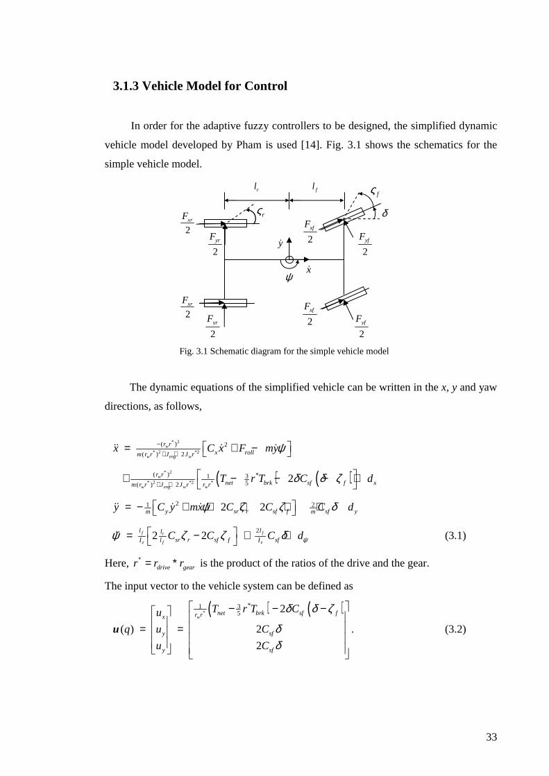
33
3.1.3 Vehicle Model for Control
In order for the adaptive fuzzy controllers to be designed, the simplified dynamic
vehicle model developed by Pham is used [14]. Fig. 3.1 shows the schematics for the
simple vehicle model.
Fig. 3.1 Schematic diagram for the simple vehicle model
The dynamic equations of the simplified vehicle can be written in the x, y and yaw
directions, as follows,
* 2
* 2 *2
( ) 2
( ) 2w
w eng w
r rx rollm r r J J r
x C x F myψ−+ +
= + − ɺɺɺ ɺ ɺ
( ) ( )* 2
* 2 *2 *
( ) *315( ) 2
2w
w eng w w
r rnet brk sf f xm r r J J r r r
T r T C dδ δ ζ+ +
+ − − − +
21 22 2y sr r sf f sf ym my C y mx C C C dψ ζ ζ δ = − + + + + + ɺɺɺ ɺ ɺ
22 2f fr
z f z
l llsr r sf f sfI l IC C C dψψ ζ ζ δ = − + +
ɺɺ (3.1)
Here, drive gearr r r∗ = ∗ is the product of the ratios of the drive and the gear.
The input vector to the vehicle system can be defined as
( ) ( )*
*315 2
( ) 2
2
wnet brk sf fr rx
y sf
y sf
T r T Cu
q u C
u C
δ δ ζ
δδ
− − − = =
u . (3.2)
2xrF
2xrF
2yrF
2yrF
2xfF
2xfF
2yfF
2yfF
δ
xɺ
yɺ
fl rl
ψɺ
fς
rς
34
T
x yd d dψ = d indicates un-modeled dynamics, modeling uncertainties and
bounded disturbances that can be demarcated as i id D≤ , ( ) 0iD ∈ >R where
, ,i x y ψ= ɺɺ ɺ .
The dynamic equations provided in (3.1), (3.2) are in terms of distance of the
centre of gravity (c.o.g.) of the vehicle from the road centreline. It has been a common
practice to describe the vehicle dynamics in terms of lateral displacement at the sensor
[14], [18], and is therefore, taken as sy . The relationship between yɺ and syɺ is
approximated as
s sy y lψ≈ + ɺɶɺ ɺ (3.3)
where desψ ψ ψ= −ɶ , and desψ is the desired yaw angle, i.e. approximate tangential angle
to the centreline of the lane. sl is the distance from the vehicle centre of gravity to the
vertical centre of the vehicle mounted sensor. Thereby, longitudinal, lateral and yaw
dynamics of (3.1) can be written as follows, respectively, in the sensor space in concise
form as
( )x s x x xx h q b u d= + +ɺɺ ɺ (3.4)
( )ss y s y y yy h q b u d= + +ɺɺ ɺ (3.5)
( ) yh q b u dψ ψ ψψ = + +ɺɺ ɺ , (3.6)
and in vector form as ( ) ( )s s sq q= + +q h bu dɺɺ ɺ where ( ) ( )sq q=u u , [ ]T
s s sx y ψ=qɺ ɺɺ ɺ ,
* 2
* 2 *2
( ) 1( ) 2
fw
zw eng w
TT lr rx y m Im r r J J r
diag b b b diagψ + + = =
b and
( )( )
* 2
* 2 *2
( ) 2
( ) 2
21
( ) ( ) ( ) ( )
2 2
2 2
s
w
w eng w
f r
z f
T
s x s y s
r rx roll s sm r r J J r
y s s sr r sf fm
l lsr r sf fI l
q h q h q h q
C x F m y l
C y l mx C C
C C
ψ
ψ ψ
ψ ψ ζ ζ
ζ ζ
−+ +
=
+ − − = − − + + + −
h ɺ ɺ ɺ ɺ
ɺɶ ɺɺ ɺ
ɺɶ ɺɺ ɺ. (3.7)
The measurement of longitudinal speed, xɺ is carried out using a wheel speed
sensor. The yaw rate of the vehicle, ψɺ is obtained using a gyroscope [18]. The
calculation of syɺ can be done using the measurements from a magnetometer and
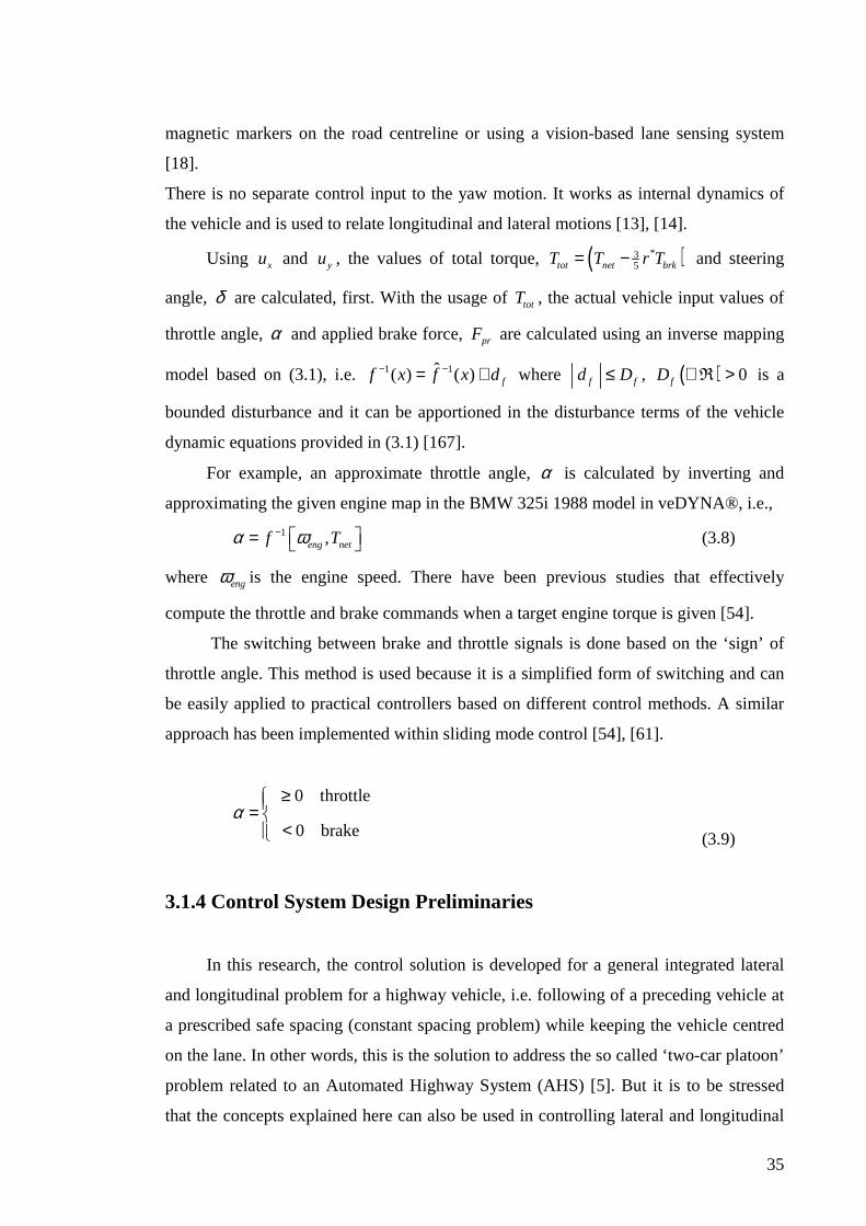
35
magnetic markers on the road centreline or using a vision-based lane sensing system
[18].
There is no separate control input to the yaw motion. It works as internal dynamics of
the vehicle and is used to relate longitudinal and lateral motions [13], [14].
Using xu and yu , the values of total torque, ( )*35tot net brkT T r T= − and steering
angle, δ are calculated, first. With the usage of totT , the actual vehicle input values of
throttle angle, α and applied brake force, prF are calculated using an inverse mapping
model based on (3.1), i.e. 1 1ˆ( ) ( ) ff x f x d− −= + where f fd D≤ , ( ) 0fD ∈ >R is a
bounded disturbance and it can be apportioned in the disturbance terms of the vehicle
dynamic equations provided in (3.1) [167].
For example, an approximate throttle angle, α is calculated by inverting and
approximating the given engine map in the BMW 325i 1988 model in veDYNA®, i.e.,
1 ,eng netf Tα ω− = (3.8)
where engω is the engine speed. There have been previous studies that effectively
compute the throttle and brake commands when a target engine torque is given [54].
The switching between brake and throttle signals is done based on the ‘sign’ of
throttle angle. This method is used because it is a simplified form of switching and can
be easily applied to practical controllers based on different control methods. A similar
approach has been implemented within sliding mode control [54], [61].
0 throttle
0 brakeα
≥= < (3.9)
3.1.4 Control System Design Preliminaries
In this research, the control solution is developed for a general integrated lateral
and longitudinal problem for a highway vehicle, i.e. following of a preceding vehicle at
a prescribed safe spacing (constant spacing problem) while keeping the vehicle centred
on the lane. In other words, this is the solution to address the so called ‘two-car platoon’
problem related to an Automated Highway System (AHS) [5]. But it is to be stressed
that the concepts explained here can also be used in controlling lateral and longitudinal

36
vehicle control aspects under normal road conditions, e.g., adaptive cruise control
coupled with lateral vehicle control.
3.1.5 Error Definitions
The longitudinal spacing error between the leading vehicle and the vehicle being
controlled is taken as xe , and the lateral deviation error from the centreline of the lane in
the sensor space is taken as ye . The error definitions can be expressed as
.
x p spacing
y d
e x x x
e y y
= − −
= − (3.10)
Here, px is the position of the leading vehicle. The desired inter-vehicular gap,
spacingx can be chosen as a function of the vehicle speed, or simply as a constant
depending on the prevailing traffic conditions [18]. These tracking error definitions are
consistent with the previous lateral and longitudinal control designs [13], [14], [17],
[18].
The desired lateral value,dy can be taken as zero as the aim is to follow the
centreline of the lane. The calculation of lateral deviation, y can be done using a
magnetometer and magnetic markers [18].

37
3.2 veDYNA® Vehicle Model for Controller Validation
3.2.1 Introduction
veDYNA® is a simulation platform with a high precision model of vehicle
dynamics based on BMW 325i, 1988 model. veDYNA® has been designed to simulate
vehicle driving properties based on the characteristics of aerodynamics, steering,
suspension, tyres, transmission, engine and drive train etc.
veDYNA® is implemented in MATLAB/Simulink® environment providing a
standard interface ensuring modular and open-model architecture. This study used
veDYNA® ‘standard’ version that offers extended possibilities to configure a
simulation model, including the configuration of separate component models for drive
train, wheel systems and tyres, engine, chassis and suspension etc. The model version
used in this study is veDYNA® 3.10.
3.2.2 veDYNA® Main Graphical User Interface
veDYNA® main dialogue that gives access to control the entire simulation
process is provided below in Fig. 3.2. This includes model data management and
adjustments of the simulation environment, i.e. settings for simulation platform and
Simulink® model. The GUI helps to configure the vehicle model: specify manoeuvre,
driver and road settings; define trace variables; start the simulation and examine the
results etc.

38
Fig. 3.2 veDYNA® main GUI
3.2.3 veDYNA® Accelerator Pedal Input (for Throttle Control)
The accelerator pedal input can be set as ‘external’, and therefore connected
through the controller setup. This is through which the accelerator pedal input of the
controllers developed in this research, is interfaced to the vehicle model. This GUI is
shown in Fig. 3.3.
Fig. 3.3 Accelerator pedal input (set as ‘external’ input) (Parent figure Fig. 3.2, ‘main GUI’)

39
3.2.4 veDYNA® Steering Angle Input (for Steering Wheel Control)
The steering angle input also can be set as ‘external’ input, and thereby, connect
through the controller setup. This is through which the steering input of the controllers
developed in this research, is interfaced to the vehicle model. This GUI is shown in Fig.
3.4.
Fig. 3.4 Steering angle input (set as ‘external’ input) (Parent figure Fig. 3.2, ‘main GUI’)
3.2.5 veDYNA® Brake Pedal Input
Similar to the other two inputs, the brake pedal input also can be set as an
‘external’, and thereby connected through from the controller setup. This is through
which the brake input of the controllers developed in this research, is interfaced to the
vehicle model. The GUI is shown in Fig. 3.5, below.

40
Fig. 3.5 Brake pedal input (set as an ‘external’ input) (Parent figure Fig. 3.2, ‘main GUI’)
3.2.6 veDYNA® Vehicle Assembly GUI
The vehicle assembly GUI, illustrated in Fig. 3.6, allows one to select the required
vehicle configuration from the list of subsystems. It also allows to interact with and
change parameters of the provided subsystems.
It is possible to navigate through the vehicle component structure by selecting a
vehicle component in the structure tree displayed on the left browser window. The
selected parameter files can be further edited. A modified or newly generated
configuration can then be saved (under a different name, if required). Some component
lines have an additional button, which generates a meaningful visualisation of the data
record, especially to verify tables or force characteristics (e.g. engine torque table,
spring characteristic, axle kinematics etc.).
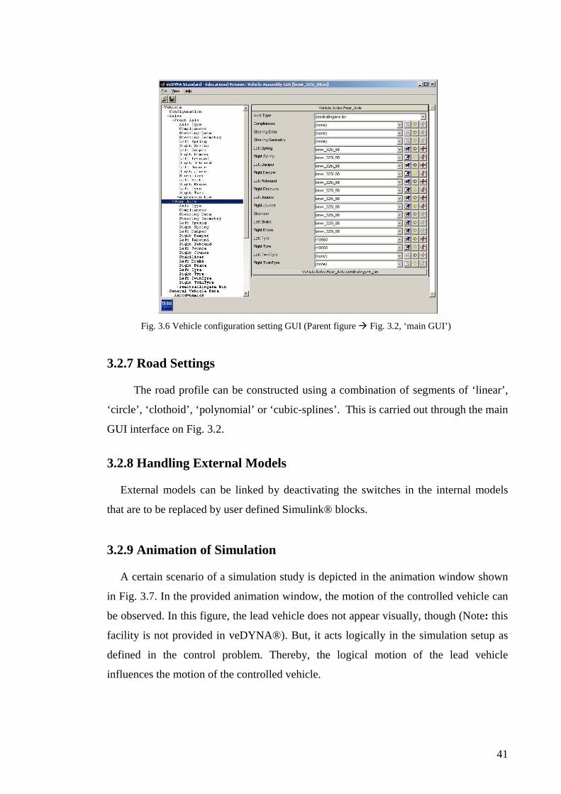
41
Fig. 3.6 Vehicle configuration setting GUI (Parent figure Fig. 3.2, ‘main GUI’)
3.2.7 Road Settings
The road profile can be constructed using a combination of segments of ‘linear’,
‘circle’, ‘clothoid’, ‘polynomial’ or ‘cubic-splines’. This is carried out through the main
GUI interface on Fig. 3.2.
3.2.8 Handling External Models External models can be linked by deactivating the switches in the internal models
that are to be replaced by user defined Simulink® blocks.
3.2.9 Animation of Simulation A certain scenario of a simulation study is depicted in the animation window shown
in Fig. 3.7. In the provided animation window, the motion of the controlled vehicle can
be observed. In this figure, the lead vehicle does not appear visually, though (Note: this
facility is not provided in veDYNA®). But, it acts logically in the simulation setup as
defined in the control problem. Thereby, the logical motion of the lead vehicle
influences the motion of the controlled vehicle.

42
Fig. 3.7 veDYNA® animation window (Parent figure Fig. 3.2 ‘main GUI’)
3.2.10 veDYNA® Simulink® Model
The veDYNA® Simulink® Model is shown in Fig. 3.8. In this figure, the block
External I/O contains pre-defined input/output (I/O) interfaces for brake hydraulics of
the vehicle as well as inputs from the engine. The block veDYNA Simulation Model is
the core of the program. Data flows to the external I/O block are via the ports ‘Output to
I/O’ and ‘Input from I/O’.
veDYNASimulation Model
vdy_mdl
External I/O
io_task
Vehicle Animation Data
Vehicle Trace DataMD Traf o
Triggered Vehicle Animation
veDYNA 3.10TESIS DYNAware GmbH
Pulse
DOC
Text
Fig. 3.8 veDYNA® Simulink® model setup
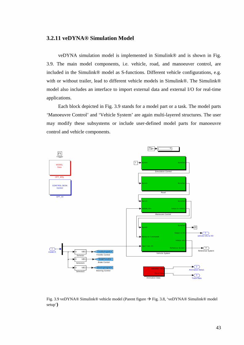
43
3.2.11 veDYNA® Simulation Model
veDYNA simulation model is implemented in Simulink® and is shown in Fig.
3.9. The main model components, i.e. vehicle, road, and manoeuver control, are
included in the Simulink® model as S-functions. Different vehicle configurations, e.g.
with or without trailer, lead to different vehicle models in Simulink®. The Simulink®
model also includes an interface to import external data and external I/O for real-time
applications.
Each block depicted in Fig. 3.9 stands for a model part or a task. The model parts
‘Manoeuvre Control’ and ‘Vehicle System’ are again multi-layered structures. The user
may modify these subsystems or include user-defined model parts for manoeuvre
control and vehicle components.
4
Reference System
3
Trace Data
2
Animation Data1
1
vehicle info to I/O
0
Sy ncIn
Maneuv er Commands
Input f rom I/O
Sy ncOut
Output to I/O
Vehicle Inf o
Ref erence Sy stem
Vehicle SystemThrottleAngleExt
Throttle Control
1
SteeringAngleExt
Steering Control
Sy ncIn Sy ncOut
Simulation Control
U U(E)
Selector2
U U(E)
Selector1
U U(E)
Selector
Sy ncIn Sy ncOut
Road
Sy ncIn
Vehicle Inf o
Sy ncOut
Output to Vehicle
Maneuver Control
MODELData
CPT_MDL
CONTROL DESKControl
CPT_IO
BrakeForceExt
Brake Control
Animation Data
Trace Data
Animation Data
Trigger
1
master:0
Fig. 3.9 veDYNA® Simulink® vehicle model (Parent figure Fig. 3.8, ‘veDYNA® Simulink® model setup’)

44
3.2.12 veDYNA® Vehicle Model Implementation: Triggered System
Since it has been found that inclusion of fuzzy systems causes the vehicle model
to look ‘stiff’ to be solved by the default ordinary differential equation solver, i.e.,
‘ode1’(Euler), the vehicle model is enclosed in a triggered system, as a solution. This
setup allows the control system to run at a sample time of 0.0005 [s] with the higher
order solver, ‘ode4’ (Runge-Kutta), while the rest of the veDYNA® system is set to
work with the original sample time (i.e. 0.01 [s]). This arrangement is shown in Fig.
3.10. This inclusion of a triggered system is a newly added feature in this simulation
setup, and is not a part of the original setup. However, this is a recommended method to
synchronise the integration schemes, i.e. by putting all veDYNA® modules into a
triggered subsystem.
COPYRIGHT 2002 by TESIS DYNAware GmbH
veDYNA Simulation Model
3
Trace Data
2
Animation Data
1
Out1
master:0
v ehicle inf o to I/O
Animation Data1
Trace Data
discrete veDYNA subsystem
Discrete PulseGenerator
1
In1
Fig. 3.10 Triggered block enclosing veDYNA® vehicle model (Parent figure Fig. 3.8, ‘main model setup’)

45
3.2.13 veDYNA® Manoeuvre Control Block
The veDYNA® ‘Manoeuvre Control’ block, grouped into the blocks ‘Manoeuvre
Scheduler’ and ‘Manoeuvre Controller’, contains all S-functions required to perform a
manoeuvre. This is shown in Fig. 3.11. Additionally, there are blocks ‘Manoeuvre’,
‘Controller Inputs’, ‘Manoeuvre Scheduler Inputs’ and ‘HCI Inputs’ that provide
necessary manoeuvre data interfaces.
COPYRIGHT 2004 by TESIS DYNAware GmbH
veDYNA Maneuver Control
2
Output to Vehicle
1
SyncOut
Vehicle Inf o Control States
Maneuver Scheduler Inputs
Sy ncIn
Next Maneuv er Flags
Control States
HCI Switches (Long, Lat, Const)
Sy ncOut
Output to Controller
Maneuver Scheduler
Longitudinal Control Inputs
Lateral Control Inputs
Driv er Inputs
Gear Control Inputs
Clutch Control Inputs
Maneuver Controller Inputs
Sy ncIn
Commands
Vehicle Inf o
Longitudinal Control Inputs
Lateral Control Inputs
Driv er Inputs
Gear Control Inputs
Clutch Control Inputs
HCI manCtrl
Sy ncOut
Output to Vehicle
Next Maneuv er Flags
Maneuver Controller
HCI Switches
HCI Switches
HCI manCtrl
HCI Switch Driver
2
Vehicle Info
1
SyncIn
Fig. 3.11 veDYNA® manoeuvre control block (Parent figure Fig. 3.9, ‘veDYNA® Simulink® vehicle model’)
3.2.14 Manoeuvre Controller Inputs
The manoeuvre controller inputs can be fed through the relevant blocks in the
‘Manoeuvre Controller Inputs’, as shown below in Fig. 3.12.
5
Clutch Control Inputs
4
Gear Control Inputs
3
Driver Inputs
2
Lateral Control Inputs
1
Longitudinal Control Inputs
Longitudinal Control Inputs
Longitudinal Control Inputs
Lateral Control Inputs
Lateral Control Inputs
Gear Control Inputs
Gear Control Inputs
Driv er Inputs
Driver Inputs
Clutch Control Inputs
Clutch Control Inputs
Fig. 3.12 Manoeuvre controller input block (Parent figure Fig. 3.11, ‘veDYNA® manoeuvre control block’)

46
3.2.15 Longitudinal Control Inputs
The longitudinal control inputs, ‘throttle angle’ and ‘brake pedal position’ are fed
through the ‘longitudinal control inputs’ blocks, as shown below in Fig. 3.12
1
Longitudinal Control Inputs
[ThrottleAngleExt]
Throttle Angle Input
1/3.6
Scale to [m/s]
1
Scale to [0..1]1
1
Scale to [0..1]
Value[1]
SW_ManLongCtrl_1_LongManMode
IO Port
OtherValue[Other]
PAR_ManLongCtrl_1_Throttle
IO Port
OtherValue[CDESK [Value]]
PAR_ManLongCtrl_1_Speed
IO Port
OtherValue[CDESK [Value]]
PAR_ManLongCtrl_1_EngineTorque
IO Port
OtherValue[Other]
PAR_ManLongCtrl_1_Brake
IO Port
OtherValue[CDESK [Value]]
PAR_ManLongCtrl_1_AccelerationY
[BrakeForceExt]
Brake Pedal Input
Fig. 3.13 Longitudinal control input (Parent figure Fig. 3.12, ‘Manoeuvre controller input block’) 3.2.16 Lateral Control Inputs
The lateral control input, ‘steering angle’, is fed through the ‘lateral control
inputs’ block, as shown below in Fig. 3.13.
1
Lateral Control Inputs[SteeringAngleExt]
Steering Angle Input
pi/180
Scale to [rad]
Value[4]
SW_ManLatCtrl_1_Steering
IO Port
OtherValue[Other]
PAR_ManLatCtrl_1_Steering
IO Port
OtherValue[CDESK [Value]]
PAR_ManLatCtrl_1_Curvature
Fig. 3.14 Lateral control input (Parent figure Fig. 3.12, ‘Manoeuvre controller input block’)

47
3.2.17 External Controller Interface to veDYNA®
The developed controller setup (‘blue coloured’) is interfaced to the veDYNA®
Simulink® setup using the following block shown in Fig. 3.15.
1
to veDYNA
ASR Flag
ASR Torque
MSR Flag
MSR Torque
RFP1 on/of f [0..1] Vehicle
USV1 [A] Vehicle
HSV1 [A] Vehicle
EVVL [A] Vehicle
AVVL [A] Vehicle
EVHR [A] Vehicle
AVHR [A] Vehicle
RFP2 on/of f [0..1] Vehicle
USV2 [A] Vehicle
HSV2 [A] Vehicle
EVVR [A] Vehicle
AVVR [A] Vehicle
EVHL [A] Vehicle
AVHL [A] Vehicle
RFP1 on/of f [0..1] Trailer
USV1 [A] Trailer
HSV1 [A] Trailer
EVVL [A] Trailer
AVVL [A] Trailer
EVHR [A] Trailer
AVHR [A] Trailer
RFP2 on/of f [0..1] Trailer
USV2 [A] Trailer
HSV2 [A] Trailer
EVVR [A] Trailer
AVVR [A] Trailer
EVHL [A] Trailer
AVHL [A] Trailer
to v eDYNA
veDYNA Standard Vehicle I/O
Chassis - 1infos_v - vspb - [3]
Write To WorkSpace1
Driver - 1veh_state - yaw_angle - [1]
Write To WorkSpace
x
y
psi
<alpha>
<Fpr>
Vehicle Controller Setup
U U(E)
Selector1
U U(E)
Selector
Chassis - 1infos_v - vspb - [3]
Read From WorkSpace3
Driver - 1veh_state - yaw_angle - [1]
Read From WorkSpace
1s
Integrator2
1s
Integrator1
DOC
Text
Demux
Demux
Demux
1
from veDYNA
Fig. 3.15 Control input interface to veDYNA® blocks (Parent figure Fig. 3.8, ‘External I/O / veDYNA Simulink model’)
3.2.18 Settings for External Disturbances for Vehicle System
The following external disturbances can be setup in the veDYNA® system using
the interfaces provided as described below.
(i) Unsymmetrical Load Mass With addition of an unsymmetrical load mass, the resulting ‘second moment of
area’ and ‘centre of gravity’ values are needed to be specified in the veDYNA® system.
Therefore, the particular new values are defined with respect to the reference axes of the
vehicle, in the relevant m-file (with parameters on load mass) as accessed from the
veDYNA® Vehicle Assembly GUI. This particular program script is shown below. The

48
schematic diagram providing the relative dimensions of the location of the load mass is
shown in Fig. 3.16.
Fig. 3.16 Unsymmetrical load mass arrangement (Note: Figure dimensions are not to proportion)
The part of the program script of the m-file defining ‘centre of gravity’ and
‘second moment of area’ values, is shown below in (3.11).
“
massl = 200; % default 0.0; % [kg] mass
rblk(1) = -2.0; % default 0.0; % [m] x-value CG
rblk(2) = 0.5; % default 0.0; % [m] y-value
rblk(3) = 0.1; % default 0.0; % [m] z-value CG (3.11)
ttlk(1) = 1.33; % default 0.0; % [kgm**2] xx
ttlk(3) = 3.33; % default 0.0; % [kgm**2] yy
ttlk(6) = 3.33; % default 0.0; % [kgm**2] zz
mainbody_flag = 1; % default 0;
” The moment of inertia values, i.e., ,xx yyI I and zzI with respect to the x, y and z
axes were calculated based on the dimensions and the mass of the load.
(ii) Crosswind Effects
In order to set a uniform crosswind speed of 50 [m/s] in the system, the relevant
program file, an m-file (with parameters on aerodynamics of the vehicle), was adjusted
in the veDYNA® Vehicle Assembly GUI. The specific program script is shown below
in (3.12).
y
z x
C.G. 2.0 m
0.1 m
0.5 m
dimensions: [0.4 0.2 0.2× × ] m mass: 200 kg
vehicle longitudinal axis

49
“vwind0 = [0.0, 50.0, 0.0]; % constant wind velocity vector provided
in inertial system, default: [0 0 0] [m/s] ”
(3.12)
(iii) Tyre-Road Friction Change
In order to simulate a friction change event, the tyre-road friction coefficient was
set to 0.5 (from normal 1.0 value) only for the segment of the road that starts at 100 [m]
and runs through up to 200 [m] using the window of ‘z-profile setting’ under ‘Advanced
Road’ section. This setting is shown below in Fig. 3.17.
Fig. 3.17 z-profile setting window (Parent figure Fig. 3.2, ‘veDYNA® main GUI’)
3.2.19 Settings for Failure Modes (Non-Catastrophic)
The following failure mode cases were set by using additional function blocks
provided in the veDYNA® library. Some changes were done as and when necessary in
order to obtain the particular simulation setting.
(i) Sudden Tyre Deflation Incident
In order to create a sudden tyre deflation incident, an external ‘flat tyre block’ (a
veDYNA® library block) was added to the ‘veDYNA Simulink Vehicle Model’, as
shown in Fig. 3.18 below. With the execution of the ‘script’ that follows, it is possible
for the system to disable the internal tyre block arrangement, and thereby switch the
control to the external tyre block.
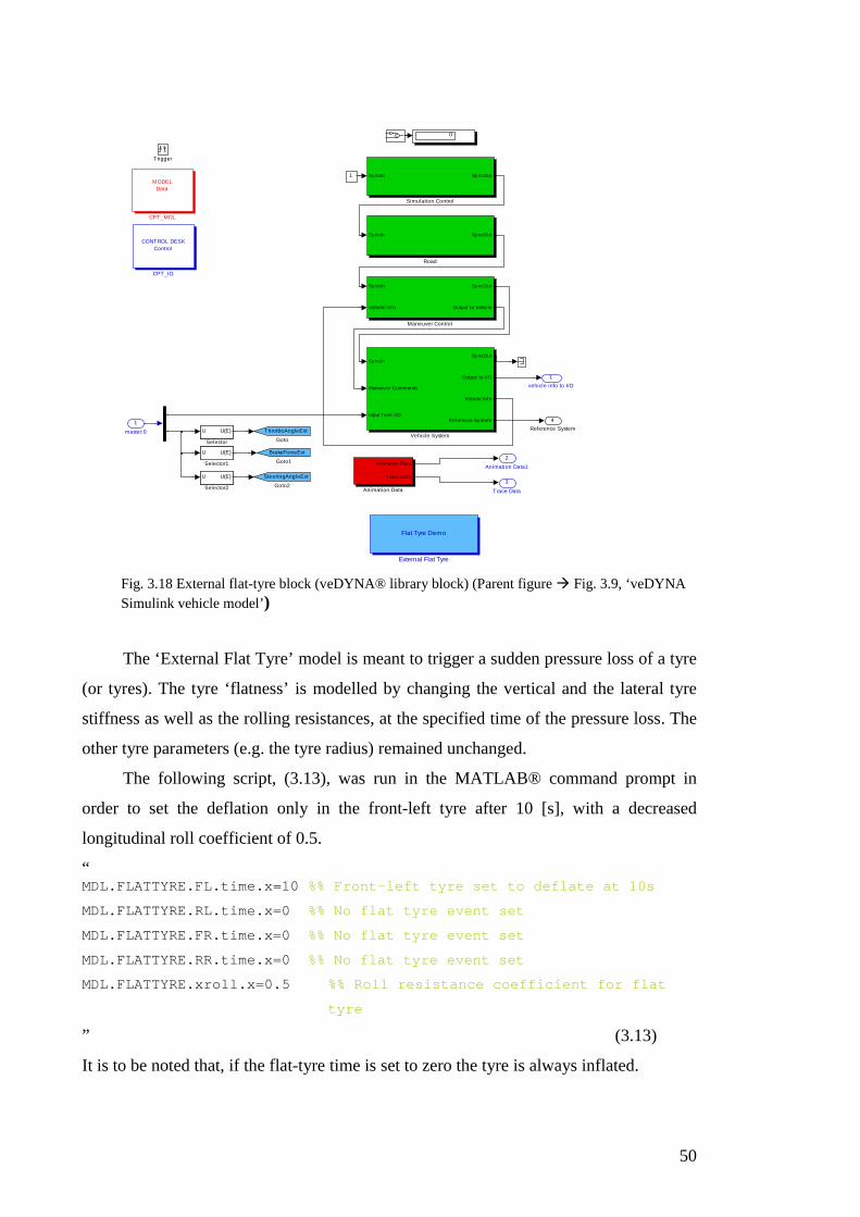
50
4
Reference System
3
Trace Data
2
Animation Data1
1
vehicle info to I/O
0
Sy ncIn
Maneuv er Commands
Input f rom I/O
Sy ncOut
Output to I/O
Vehicle Inf o
Ref erence Sy stem
Vehicle System
1 Sy ncIn Sy ncOut
Simulation Control
U U(E)
Selector2
U U(E)
Selector1
U U(E)
Selector
Sy ncIn Sy ncOut
Road
Sy ncIn
Vehicle Inf o
Sy ncOut
Output to Vehicle
Maneuver Control
SteeringAngleExt
Goto2
BrakeForceExt
Goto1
ThrottleAngleExt
Goto
Flat Tyre Demo
External Flat Tyre
MODELData
CPT_MDL
CONTROL DESKControl
CPT_IO
Animation Data
Trace Data
Animation Data
Trigger
1
master:0
Fig. 3.18 External flat-tyre block (veDYNA® library block) (Parent figure Fig. 3.9, ‘veDYNA Simulink vehicle model’)
The ‘External Flat Tyre’ model is meant to trigger a sudden pressure loss of a tyre
(or tyres). The tyre ‘flatness’ is modelled by changing the vertical and the lateral tyre
stiffness as well as the rolling resistances, at the specified time of the pressure loss. The
other tyre parameters (e.g. the tyre radius) remained unchanged.
The following script, (3.13), was run in the MATLAB® command prompt in
order to set the deflation only in the front-left tyre after 10 [s], with a decreased
longitudinal roll coefficient of 0.5.
“ MDL.FLATTYRE.FL.time.x=10 %% Front-left tyre set to deflate at 10s
MDL.FLATTYRE.RL.time.x=0 %% No flat tyre event set
MDL.FLATTYRE.FR.time.x=0 %% No flat tyre event set
MDL.FLATTYRE.RR.time.x=0 %% No flat tyre event set
MDL.FLATTYRE.xroll.x=0.5 %% Roll resistance coefficient for flat
tyre
” (3.13)
It is to be noted that, if the flat-tyre time is set to zero the tyre is always inflated.

51
(ii) Defective Wheel Brake Cylinder (front-left wheel) In order to simulate a pressure drop in the brake line leading to front-left wheel
cylinder, an external brake system block (a veDYNA® library block) was added to the
‘Vehicle System’ block of ‘veDYNA Simulink Vehicle Model’. This is shown in Fig.
3.19. With the execution of the ‘script’ that follows, it is possible to disable the internal
tyre block arrangement, and thereby, switch the control to the external block.
COPYRIGHT 2002 by TESIS DYNAware GmbH
veDYNA Vehicle System
4
Reference System
3
Vehicle Info
2
Output to I/O
1
SyncOut
Sy ncIn
Maneuv er Commands
Input f rom I/O
External Body Forces
Output to I/O
Vehicle Inf o
Ref erence Sy stem
Sy ncOut
Ref erence Sy stem1
<veDYNA Vehicle>
System Instance [1]
veDYNA Vehicle Subsystem
Brake Demo
External Brake System
3
Input from I/O
2
Maneuver Commands
1
SyncIn
Fig. 3.19 External brake system block (veDYNA® library block) (Parent figure Fig. 3.9, ‘veDYNA Simulink vehicle model’)
The following script, (3.14) is run in the MATLAB® command prompt in order to
disable the internal brake system while activating the external brake system.
“ MDL.EXTBRK.rbr.ft.v=0.105 %% set with the same parameters as the
internal
MDL.EXTBRK.rbr.rr.v=0.105 %% set with the same parameters as the
internal
MDL.EXTBRK.abrk.ft.v=1.8E-3 %% set with the same parameters as the
internal
MDL.EXTBRK.abrk.rr.v=1.8E-3 %% set with the same parameters as the
internal
MDL.EXTBRK.muebr.ft.v=0.35 %% set with the same parameters as the
internal
MDL.EXTBRK.muebr.rr.v=0.35 %% set with the same parameters as the
internal
MDL.EXTBRK.t0.v=0 %% time delay to reaction time of the wheel brake

52
MDL.EXTBRK.onoff.v=1 %% Vehicle switched to external brake system
from the internal brake system ”
(3.14)
In the activated external brake system, the defect in the front-left wheel cylinder
was modelled as shown in Fig. 3.20. The defect in the front-left wheel cylinder was
simulated by reducing the pressure of the brake line by 90% from the normal value. The
pressure lines of the other wheel cylinders were assumed to remain as normal during the
simulation.
1
Control
1
Gain4
1
Gain3
0.1
Gain2
1
Gain1
0.25
EXTBRK.onoff.v
External brakeson/off switch
EXTBRK.onoff.v
External Switch
PressureTorque
Info
Disc Brake Wheel 4
PressureTorque
Info
Disc Brake Wheel 3
PressureTorque
Info
Disc Brake Wheel 2
PressureTorque
Info
Disc Brake Wheel 1
Demux
0
Wheel 8
0
Wheel 7
0
Wheel 6
0
Wheel 5
1
States
Fig. 3.20 External brake system-brake lines (with the front-left wheel cylinder set as defective with 90% pressure drop in the brake line) (Parent figure Fig. 3.19 External brake system block)
3.2.20 Calculation of h Value for veDYNA® Vehicle Model
The value of h as indicated by (3.7) is required for the analysis of the simulation
and for data collection in the design of the fuzzy systems. Therefore the value of h of
the veDYNA® model can be calculated using the following equation.
( )
( )x s x x
y s y y
h q x b u
h q y b u
= −= −
ɺ ɺɺ
ɺ ɺɺ (3.15)
The values of xɺɺ and yɺɺ can be obtained from the vehicle model sensor feedback.
This is possible since xb and yb are known, and the control inputs xu and yu can be
calculated.

53
3.3 Chapter Summary
In the first part of this chapter, a simple vehicle model to be used in the design of
all control systems in this research is described in detail. This description also includes
details on throttle/brake switching criterion used in the design of the controllers.
In the second part of the chapter, a veDYNA® setup, a simulation platform
providing a high-precision vehicle model that is used as the validation platform with
simulations for all the controllers developed in this research, is described in detail. This
description includes all GUIs, interfaces and setups related to veDYNA® under
different conditions of working of the vehicle for simulating vehicle control operations.

54
55
C H A P T E R 4
Robust Single-Model Adaptive Fuzzy Control System In this chapter, the development of a single-model adaptive fuzzy controller for
integrated lateral and longitudinal control of highway vehicles is described. The single-
model adaptive fuzzy system is comprehensively designed and its parameters are tuned
using a subtractive clustering method, first, and then the ANFIS (Adaptive Networks
Fuzzy Inference Systems) method for fine adjustments. Following tuning, the system of
single-adaptive fuzzy control is established with stability analysis using a Lyapunov-
based method, i.e. KYP lemma, leading to asymptotic stability at global level. Finally,
the developed controller is tested for its robust qualities with validation studies using
simulations in veDYNA®, exposing the controller to a number of robust conditions,
including a few external disturbances and a couple of non-catastrophic failure cases of
vehicle subsystems.

56
4.1 Robust Single-Model Adaptive Fuzzy Control System
4.1.1 Introduction
Vehicle control, especially involving integrated lateral and longitudinal control,
has to deal with significant nonlinearity effects. According to the details highlighted in
the main introduction, vehicle systems require specialized controllers.
In order to address the nonlinearity effects, and other uncertainty effects in vehicle
control problems, a single adaptive fuzzy controller is designed as described in this
chapter. The control system also contains a proportional-derivative (PD) module, which
is important for coarse tuning in the solution of control problem. On the other hand,
adaptive fuzzy system is for robust tuning or fine tuning of the controller addressing
non-linearity effects, coupling effects, and model uncertainties.
4.1.2 Synthesis of Single-Adaptive Fuzzy Controller
In this section, the synthesis of a single-model adaptive fuzzy controller system is
described. The PD module in the control system is for tracking linear components of
the vehicle system. The fuzzy system is employed to address nonlinear components of
the control problem. These nonlinear effects involve coupling effects, model
discrepancies, and un-modelled dynamics. In addition to these modules, a variable
structure control term is used in the control system for specifically addressing fuzzy
approximation errors, and to overcome disturbances to certain extent.
Instead of using a PD module, if an integral component (I) was included in the
system, e.g. as a PI system or as a PID system, the control system might be more
susceptible to what is called a ‘winding up’ problem. In other words, the closed loop
system would become unresponsive, and therefore lead to look like an open loop
system. This whole phenomenon where there is a discrepancy between the controller
output and the plant input due to actuator saturation is called integrator or controller
windup in literature [168]. This phenomenon is due to the fact that in real-world
controlled engineering systems, actuator capacity is limited by the inherent physical

57
constraints. In other words, actuators are confined to operate between certain saturation
limits. This windup problem could result in a significant performance degradation, large
overshoots or un-decaying transients. There is a more tendency of the integral
controllers (PI or PID) to ‘windup’ during input saturation. In order to prevent this
happening with the inclusion of an integral component in the controller, it is required to
use an anti-windup module. But, this addition would increase the nonlinearity of the
system, and therefore would require more complex analysis for establishing stability.
This becomes a much more challenging problem in a complex nonlinear system [169].
In order to avoid these complexities, a PD system was used in this research without
including any integral component.
(i) Control Law
The certainty equivalence control laws based on adaptive fuzzy control and
proportional-derivative components can be formulated for longitudinal and lateral cases,
respectively, as follows.
1 ˆˆˆ ( )x p dx x px x x sx x sx
u x k e k e u h qb
ν = + + + + − ɺɺ ɺ ɺ (4.1)
1 ˆˆˆ ( ) .sy s dy y py y y sy y s
y
u l k e k e u h qb
ψ ν = + + + + − ɺɺɶ ɺ ɺ (4.2)
Here, ,ˆ ( )
sx y sh qɺ denotes the calculated value of the term , ( )sx y sh qɺ . ˆxν and ˆyν are
the inputs from the adaptive fuzzy controller for longitudinal and lateral cases,
respectively. dxk , pxk are the constant PD (proportional-derivative) gains for the
longitudinal control, and dyk , pyk are the constant PD gains for the lateral control.
s sx syu u u = is the variable structure control term.
(ii) Error Dynamics
The control inputs from (4.1) can be substituted in the vehicle model equation
(3.4) of Chapter 3, and it can be rearranged to have the longitudinal error dynamics as
ˆ ˆ( ) ( )x dx x px x x s x s x sx xe k e k e h q h q u dν+ + = − − − −ɺɺ ɺ ɺ ɺ . (4.3)
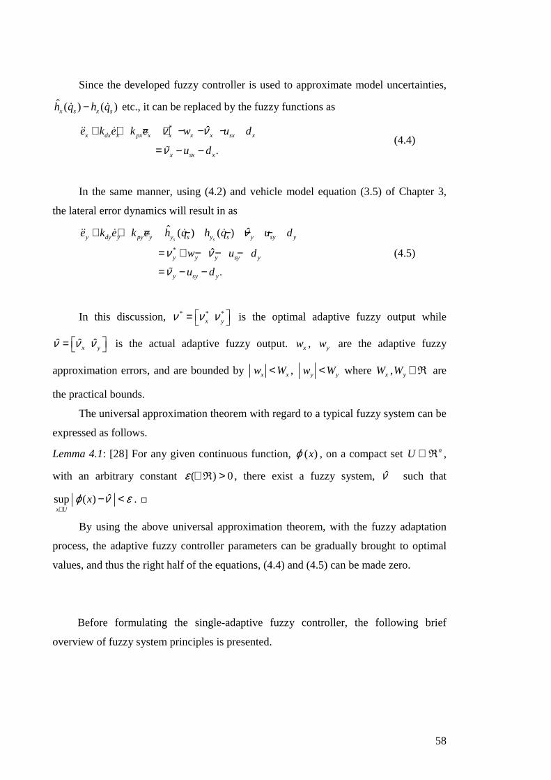
58
Since the developed fuzzy controller is used to approximate model uncertainties,
ˆ ( ) ( )x s x sh q h q−ɺ ɺ etc., it can be replaced by the fuzzy functions as
* ˆ
.
x dx x px x x x x sx x
x sx x
e k e k e w u d
u d
ν ν
ν
+ + = + − − −
= − −
ɺɺ ɺ
ɶ (4.4)
In the same manner, using (4.2) and vehicle model equation (3.5) of Chapter 3,
the lateral error dynamics will result in as
*
ˆ ˆ( ) ( )
ˆ
.
s sy dy y py y y s y s y sy y
y y y sy y
y sy y
e k e k e h q h q u d
w u d
u d
ν
ν νν
+ + = − − − −
= + − − −
= − −
ɺɺ ɺ ɺ ɺ
ɶ
(4.5)
In this discussion, * * *x yν ν ν = is the optimal adaptive fuzzy output while
ˆ ˆ ˆx yν ν ν = is the actual adaptive fuzzy output. xw , yw are the adaptive fuzzy
approximation errors, and are bounded by x xw W< , y yw W< where xW , yW ∈R are
the practical bounds.
The universal approximation theorem with regard to a typical fuzzy system can be
expressed as follows.
Lemma 4.1: [28] For any given continuous function, ( )xϕ , on a compact set U ∈ nR ,
with an arbitrary constant ( ) 0ε ∈ >R , there exist a fuzzy system, ν such that
ˆsup ( )x U
xϕ ν ε∈
− < .
By using the above universal approximation theorem, with the fuzzy adaptation
process, the adaptive fuzzy controller parameters can be gradually brought to optimal
values, and thus the right half of the equations, (4.4) and (4.5) can be made zero.
Before formulating the single-adaptive fuzzy controller, the following brief
overview of fuzzy system principles is presented.

59
4.1.3 Fuzzy Control: Takagi-Sugeno (T–S) Fuzzy Systems
A brief description of general fuzzy systems and T–S fuzzy system is presented.
This brief is almost reproduced here as described by Passino and Yurkovich in [28].
(i) Fuzzy System Elements
Generally, a fuzzy controller is composed of the following four main elements.
1. A rule-base that holds the knowledge (in the form of a set of IF-THEN rules)
that contains a fuzzy logic quantification of the controller engineer’s linguistic
description of how to achieve good control.
2. An inference mechanism (also called an “inference engine” or “fuzzy
inference” module) that evaluates which control rules are relevant at the current
moment, and also that emulates design engineer’s decision making in interpreting and
applying knowledge about how best to control the vehicle.
3. A fuzzification interface that converts or modifies controller inputs into
information by means of mapping the inputs to a defined so called ‘membership
function’ so that they can be easily interpreted and compared to the rules in the rule
base.
4. A defuzzification interface that converts the conclusions reached by the
inference mechanism into the actual inputs to the plant (vehicle).
(ii) Fuzzy System Concepts
The concepts related to fuzzy systems are described below.
(a) Fuzzy System
A fuzzy system (normally) is a static nonlinear mapping between its inputs and
outputs (i.e. it is not a dynamic system). It is assumed that the fuzzy system has inputs
i iu U∈ where 1, ,i n= … and outputs i iy Y∈ where 1, ,i m= … . The inputs and outputs
are crisp values, i.e. real numbers as against being fuzzy sets. The fuzzification process
converts the crisp inputs to fuzzy sets while the inference mechanism uses the fuzzy
rules in the rule-base to produce fuzzy conclusions. Finally, the defuzzification block

60
converts these fuzzy conclusions into the crisp outputs so that they can be used by real-
world systems.
(b) Universes of Discourse
The ordinary sets or crisp sets, iU and iY are called the “universes of discourse”
or domains for iu and iy , respectively. In practical applications, most often the
universes of discourse are simply the set of real numbers or some interval or subset of
real numbers. Also, sometimes it is convenient to refer to an “effective” universe of
discourse [ , ]α β where α and β are the points at which the outermost membership
functions saturate for input universes of discourse, or the points beyond which the
outputs will not move for the output universe of discourse.
(c) Linguistic Variables
To specify rules for the rule-base, the design engineers will use a ‘linguistic
description’, hence, linguistic expressions are needed for the inputs and outputs and the
characteristics of the inputs and outputs. The ‘linguistic variables’ or constant symbolic
descriptions of general time-varying quantities are used to describe fuzzy system inputs
and outputs.
(d) Linguistic Values
Linguistic variables iuɶ and iyɶ take on ‘linguistic values’ that are used to describe
characteristics of the variables. Let jiAɶ denote the jth linguistic value of the linguistic
variable iuɶ defined over the universe of discourse iU . If it is assumed that many
linguistic values are defined over iU , then the linguistic variable iuɶ takes on the
elements from the set of linguistic values as defined by
: 1, 2, ,ji i iA A j N= =ɶ … . (4.6)
Linguistic values are generally descriptive terms such as “positive large”, “zero”, and
“negative large” etc.

61
(e) Linguistic Rules
The mapping of the inputs to the outputs for a fuzzy system is in part
characterized by a set of condition → action rules, or in modus ponens (If-Then) form,
If premise Then consequent.
Usually, the inputs of the fuzzy system are associated with the premise, and the
outputs are associated with the consequent. These If-Then rules can be represented in a
number of forms, e.g. multi-input-single-output (MISO) or multi-input-multi-output
(MIMO) etc. The MISO form of a linguistic rule for a standard system (Mamdani) is,
If 1uɶ is 1jAɶ and 2uɶ is 2
kAɶ and , . . . , and nuɶ is lnAɶ Then qyɶ is pBɶ (4.7)
But, for a functional fuzzy system where T–S (Takagi-Sugeno) type is a special
case, it becomes
If 1uɶ is 1jAɶ and 2uɶ is 2
kAɶ and , . . . , and nuɶ is lnAɶ Then ( )i ib g= • . (4.8)
The difference between a standard fuzzy system and a T–S fuzzy system is in the
consequent part. The premise parts are similar in construction. Here, ib can be any
function, but linear or affine functions are mostly used.
(f) Membership Functions
Let iU denote a universe of discourse and ji iA A∈ɶ ɶ denote a specific linguistic
value for the linguistic variable iuɶ . The function ( )iuµ associated with jiAɶ that maps
iU to [0, 1], is called a ‘membership function’. This membership function quantifies
the “certainty” that an element of iU , denoted iuɶ , can be classified linguistically as jiAɶ .
Membership functions are subjectively specified in an ad-hoc (heuristic) manner from
experience or intuition.

62
(g) Fuzzy Sets
Given a linguistic variable iuɶ with a linguistic value jiAɶ defined on the universe
of discourse iU , and membership function ( )iA iuµ (membership function associated
with the fuzzy set jiA ) that maps iU to [0, 1], a “fuzzy set” denoted with j
iA is defined
as ( ) , ( ) :i
ji i A i i iA u u u Uµ= ∈ (Note: a fuzzy set is simply a crisp set of pairings of
elements of the universe of discourse coupled with their associated membership values).
(h) Fuzzification
Fuzzy sets are used to quantify the information in the rule-base, and the inference
mechanism operates on fuzzy sets to produce fuzzy sets, hence, it is required to specify
how the fuzzy system will convert its numeric inputs i iu U∈ into fuzzy sets (a process
called ‘fuzzification’) so that they can be used by the fuzzy system.
Let *iU denote the set of all possible fuzzy sets that can be defined on iU . Given
i iu U∈ , fuzzification transforms iu to a fuzzy set denoted by fuziA defined on the
universe of discourse iU . This transformation is produced by the fuzzification operator
F defined by
F: iU → *iU (4.9)
where F ˆ( ) fuzi iu A= .
Quite often, ‘singleton fuzzification’ is used, which produces a fuzzy set *ˆ fuzi iA U∈ with
a membership function defined by
ˆ
1( )
0 otherwisefuz
i
i
A
x uxµ
==
. (4.10)
Any fuzzy set with this form for its membership function is called a ‘singleton’.
(i) The Inference Mechanism
The inference mechanism has two basic tasks:

63
(1) Determining the extent to which each rule is relevant to the current situation as
characterized by the inputs iu , 1, ,i n= … (this task is called ‘matching’), and
(2) Drawing conclusions using the current inputs iu and the information in the rule-base
(this is called an ‘inference step’). For matching, note that 1 2j k lnA A A× ×⋯ is the fuzzy
set representing the premise of the ith rule ( , , , ; , )ij k l p q… (there may be more than
one such rule with this premise).
(j) Matching
If the inputs are taken as iu , 1, ,i n= … , and fuzzification produces
1 2ˆ ˆ ˆ, , ,fuz fuz fuz
nA A A… (the fuzzy sets representing the inputs), then there are two basic steps
to matching.
Step 1: Combine Inputs with Rule Premises:
The first step in matching involves finding fuzzy sets 1 2ˆ ˆ ˆ, , ,j k lnA A A… with
membership functions
fuz11 1
ˆ ˆ1 1 1( ) ( )* ( )jj
AA Au u uµ µ µ=
fuz22 2
ˆ ˆ2 2 2( ) ( )* ( )kk
AA Au u uµ µ µ= (4.11)
⋯
fuzˆ ˆ( ) ( )* ( )lnln n
n A n nA Au u uµ µ µ=
(for all , , ,j k l… )
As with singleton fuzzification, it gives fuzˆ ( ) 1i
iAuµ = for all 1, ,i n= … for the given
iu inputs, so that
11ˆ 1 1( ) ( )
jjAA
u uµ µ=
22ˆ 2 2( ) ( )
kkAA
u uµ µ= (4.12)
⋯
ˆ ( ) ( )lnln
n A nAu uµ µ= .

64
Step 2: Determine which rules are on:
In the second step, the membership values ( )1 2, , ,i nu u uµ … can be formed for the
ith rule’s premise that represents the certainty that each rule premise holds for the given
inputs. Define
( )1 2
ˆ ˆ ˆ1 2 1 2, , , ( ) ( ) ( )j k ln
i n nA A Au u u u u uµ µ µ µ= ∗ ∗ ∗… … , (4.13)
which is simply a function of the inputs iu . When singleton fuzzification is used, it can
be reduced to have
( )1 21 2 1 2, , , ( ) ( ) ( )
j k lni n A A A nu u u u u uµ µ µ µ= ∗ ∗ ∗… … . (4.14)
Here, ( )1 2, , ,i nu u uµ … is used to represent the certainty that the premise of rule i
matches the input information when singleton fuzzification is used.
An implied fuzzy set can be defined for a standard fuzzy system. But this step is
not considered for functional fuzzy systems, since the consequent is not a fuzzy
linguistic function.
(k) Defuzzification
A number of defuzzification strategies exist for standard fuzzy systems, e.g.
centre-average method. As far as the scope of this research is concerned, the
defuzzification of T–S fuzzy systems can be considered with a similar ‘centre-average’
method, as follows,
1
1
R
i iiR
ii
by
µ
µ=
=
= ∑∑
(4.15)
where iµ is as provided in (4.14).
(l) T–S Fuzzy Systems
In this research, mainly T–S fuzzy systems based on Gaussian input fuzzy
functions are used to construct adaptive fuzzy controllers and fuzzy ‘blending’ (soft-

65
switching systems) structures. In adaptive controller structures, the input fuzzy function
parameters are kept fixed while making the output membership function parameters,
i.e., the functional members, as adaptive. Generally, the ‘blending’ fuzzy structures are
non-adaptive in form as used in this research.

66
4.1.4 Design of Single-Adaptive Fuzzy Controller
In this section, the synthesis of a robust single-adaptive fuzzy controller in solving
the integrated lateral and longitudinal control problem of highway vehicles is described.
Fig. 4.1 explains the setup for each adaptive fuzzy controller with reference to the
equations (4.1) and (4.2). The term, ( )ˆx yν is the adaptive fuzzy output.
In this adaptive fuzzy control system, in addition to the basic architecture of a
fuzzy controller, an adaptation algorithm is used for updating the output membership
function parameters. The input fuzzy set parameters are kept fixed throughout.
Fig. 4.1 Adaptive fuzzy system and PD module for longitudinal (lateral) vehicle controller
There are two inputs (lateral and longitudinal) for each adaptive fuzzy controller,
i.e., the ‘error’ , e and the ‘error rate’, eɺ . The adaptive fuzzy function output, ν ∈R is
obtained after defuzzification as a crisp value, and is fed together with the inputs from
the PD control module to the vehicle. A variable structure control term, su is
incorporated into the control system for addressing fuzzy approximation errors and
thereby to ensure system stability.
The usage of fuzzy control instead of variable structure control alone can be
further justified. There is a major drawback in the variable structure control approach,
which is the phenomenon of chattering due to high frequency switching. These
chattering can often excite undesired dynamics. But fuzzy control can provide an
effective way to resolve this problem in the presence of variable structure control [170].
Moreover, fuzzy control can further provide the smoothness in operation by selecting
smooth membership functions such as Gaussian functions [171].
su
( )ˆ ( )
sx yh qɺ
ˆ ˆ( )x yu u
e
error
+
e
( )ˆ
x yν
( )p sx l ɺɶɺ ψ - +
+
Inference Mechanism
Rule Base Fuz
zific
atio
n
Def
uzzi
ficat
ion
t∆∆
+ PD
t∆∆
,1/ x yb
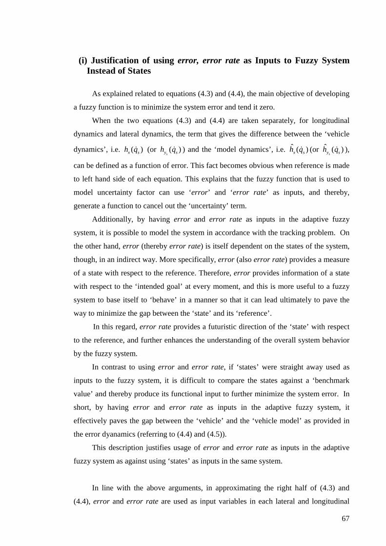
67
(i) Justification of using error, error rate as Inputs to Fuzzy System Instead of States
As explained related to equations (4.3) and (4.4), the main objective of developing
a fuzzy function is to minimize the system error and tend it zero.
When the two equations (4.3) and (4.4) are taken separately, for longitudinal
dynamics and lateral dynamics, the term that gives the difference between the ‘vehicle
dynamics’, i.e. ( )x sh qɺ (or ( )sy sh qɺ ) and the ‘model dynamics’, i.e. ˆ ( )x sh qɺ (or ˆ ( )
sy sh qɺ ),
can be defined as a function of error. This fact becomes obvious when reference is made
to left hand side of each equation. This explains that the fuzzy function that is used to
model uncertainty factor can use ‘error’ and ‘error rate’ as inputs, and thereby,
generate a function to cancel out the ‘uncertainty’ term.
Additionally, by having error and error rate as inputs in the adaptive fuzzy
system, it is possible to model the system in accordance with the tracking problem. On
the other hand, error (thereby error rate) is itself dependent on the states of the system,
though, in an indirect way. More specifically, error (also error rate) provides a measure
of a state with respect to the reference. Therefore, error provides information of a state
with respect to the ‘intended goal’ at every moment, and this is more useful to a fuzzy
system to base itself to ‘behave’ in a manner so that it can lead ultimately to pave the
way to minimize the gap between the ‘state’ and its ‘reference’.
In this regard, error rate provides a futuristic direction of the ‘state’ with respect
to the reference, and further enhances the understanding of the overall system behavior
by the fuzzy system.
In contrast to using error and error rate, if ‘states’ were straight away used as
inputs to the fuzzy system, it is difficult to compare the states against a ‘benchmark
value’ and thereby produce its functional input to further minimize the system error. In
short, by having error and error rate as inputs in the adaptive fuzzy system, it
effectively paves the gap between the ‘vehicle’ and the ‘vehicle model’ as provided in
the error dyanamics (referring to (4.4) and (4.5)).
This description justifies usage of error and error rate as inputs in the adaptive
fuzzy system as against using ‘states’ as inputs in the same system.
In line with the above arguments, in approximating the right half of (4.3) and
(4.4), error and error rate are used as input variables in each lateral and longitudinal

68
adaptive fuzzy system in this study. It is also mentioned and clarified that ‘error’ and
‘error rate’ can be used in each fuzzy rule in order to partially define the ‘states’ of a
dynamic system [28].
Remark 4.1: The advantage of taking ,e eɺ as fuzzy inputs allows effective design of the
fuzzy system. This is because the causal relationship between the inputs and fuzzy rules
are clear and straightforward. In contrast to this, if the system ‘states’ were used as
inputs to the fuzzy system, there would not be any clear way to identify the relationship
between them and the system error, even at least for initial parameters of the fuzzy
system.
(ii) Adaptive Fuzzy Systems
The detailed synthesis of the adaptive fuzzy controller is presented here. The x
and y subscripts of the two adaptive fuzzy systems for longitudinal and lateral cases,
respectively, are omitted for it to be a common construction for both lateral and
longitudinal cases.
The set of T–S fuzzy IF-THEN rules for the adaptive fuzzy system can be
expressed as
11 2: If is and is l ke A e AɺR
1 1 1Then z a e b e= + ɺ
⋮ (4.16)
: If is and is n l kn ne A e AɺR
Then ,n n nz a e b e= + ɺ
where n is the total number of fuzzy rules. ljA and kjA are the lth and kth linguistic
values associated with the linguistic variables of the inputs, e andeɺ , respectively, in the
jth rule. jz is the consequent of the jth rule where 1, ,j n= … ( ( 1)n > ∈N ). The
output membership function in the jth rule can be expressed as [ ] .T
j j jz e e a b = ɺ

69
Remark 4.2: In this subsection, x denotes the generic input element for the fuzzy
system, i.e., ,x e e= ɺ . x is used for differentiating it from the vehicle’s longitudinal
distance values, x.
The T–S fuzzy logic output with product inference, singleton fuzzifier and centre-
average defuzzifier can be expressed as
( )( )( )( )
11
11
ˆ .i
i
nm j
A i jij
nm j
A iij
x z
x
µν
µ
==
==
=∑ ∏
∑ ∏ (4.17)
The term, ( )i
jA ixµ is the fuzzy inferred input membership function value with the
ith input variable in the jth rule. It is obvious that 1, 2i = (therefore, m= 2) for ‘error’
and ‘error rate’ variables.
In concise form, the adaptive fuzzy output, ν ∈R can be stated as
ˆ ( )T xν = θξ (4.18)
where θ is the parameter vector and ( )xξ is the regression vector of the fuzzy system.
Remark 4.3: Though fuzzy system in (4.18) is generally nonlinear, it is linear with
respect to its unknown parameters. Hence, parameter adaptation algorithms applicable
for linear systems, e.g. gradient-based algorithms, can be readily used in estimation of
the unknown parameters in fuzzy systems in (4.18) [27].
The development of (4.18) is described as follows.
It can be assumed that ν , the mapping produced by the fuzzy system, is Lipschitz
continuous [30].
The jth element of the parameter vector can be provided as
T
j j ja b = θ where [ ]1 2
T
n=θ θ θ θ⋯2.n×∈R (4.19)
Let the error vector be [ ] ,T
e e=e ɺ then ( ) ( ) ( ) Tj j j jx x e x eξ ξ ξ = = eɺξ is the
jth element, for 1 , ... ,j n= , of the regression vector,
[ ]1 2( ) ( ) ( ) ( )T
nx x x x= ⋯ξ ξ ξ ξ 2n×∈R [26]. Thereby, jth regression factor (for
1 , ... ,j n= (where ( 1)n > ∈N )) can be denoted as

70
( )( )( )
1
11
( ) .i
i
m jA ii
j nm j
A iij
xx
x
µξ
µ=
==
= ∏∑ ∏
(4.20)
The adaptive fuzzy output membership function parameters of (4.18) can be tuned
using an algorithm based on the adaptive law
( )xγ= −θ Ceɺ ξ (4.21)
( [ ]1 1=C ), which is developed in the Section 4.2.4 in detail.
4.1.5 Training of Adaptive Fuzzy Controller Parameters
Tuning of input fuzzy membership function parameters were done as follows. The
parameters included Gaussian centres and standard deviations of the fuzzy system as
well the values a priori for the output membership functions. Data were collected by
carrying out six runs of trials on veDYNA® vehicle model with activating only the PD
components in the closed loop form. The six profiles included different configuration
settings (different combinations in path and curvatures, i.e., straight line, left-right turn
with maximum curvature of ± 2.29e-3 [ 1m− ] and right-left turn with maximum
curvature∓ 2.29e-3 [ 1m− ], and lead vehicle velocity variations, i.e., acceleration of 1
[ 2ms− ], fixed velocity of 10 [ 1ms− ]), with a sample rate of 0.05 [s], and a period of 20
[s] for each run.
The time period for collecting data sets was limited to 20 [s]. This is because the
output membership function parameters that are adaptive in nature need only data of
initial parts of the scenarios. But, in order to tune the fixed parts, (i.e. the centres and the
standard deviations of Gaussian membership functions), it need fairly long runs.
Nevertheless, these two parts of tuning are not possible to be done separately because it
involves a single fuzzy structure. Therefore, these two ends have been compromised,
and an initial period of 20 [s] was considered sufficient for collecting data.
With the simulation runs, the data sets consisting of inputs, i.e. error and error
rate, and the expected adaptive fuzzy output, were collected. The adaptive fuzzy output
was taken as
ˆˆ ( ) ( )i i s i sh q h qν = −ɺ ɺ , (4.22)

71
where ,i x y= , for longitudinal and lateral cases, respectively. The equation (4.22) was
obtained using (4.4) and (4.5) for longitudinal and lateral controllers, separately by
making error terms zero. The expected output of fuzzy system, ( )i sh qɺ was calculated
using output states of BMW 325i 1988 model of veDYNA®, and ˆ ( )i sh qɺ was calculated
using (3.7).
The design of fuzzy structure of each longitudinal and lateral adaptive controller
was carried out as follows. First, subtractive clustering method was used in order to find
the number of clusters [172], thereby the number of input membership functions. In
order for that, cluster radii of 0.4 (provides a measure how close the clusters would be)
for the lateral case, and 0.5 for the longitudinal case, were used separately. Subtractive
clustering also provided the preliminary structure for the adaptive fuzzy systems. Once
these membership functions were identified, IF-THEN rules for the fuzzy system were
formed by considering all the combinations of these membership functions. The fuzzy
systems were further tuned using an ANFIS (Adaptive Network Fuzzy Inference
System) system written in C++ [173]. The ANFIS system, a neuro-fuzzy structure for
tuning a given fuzzy system on a provided data set, is an offline tuning method and is
used for obtaining the primary form of a fuzzy system. Subsequently,
MATLAB/Simulink® based ‘ANFIS tool’ was used to visualize the rules and to
generate control surfaces. The MATLAB/Simulink® based ANFIS tool was not used
for further tuning purposes of the fuzzy system because it cannot be used for ‘linear
functions’ as used in this study, and provided in (4.16).
(i) Data Collection
The Simulink® model shown in Fig. 4.2, was used to collect data from special
runs on veDYNA®. The profiles used to collect the preliminary data are shown in
detail.
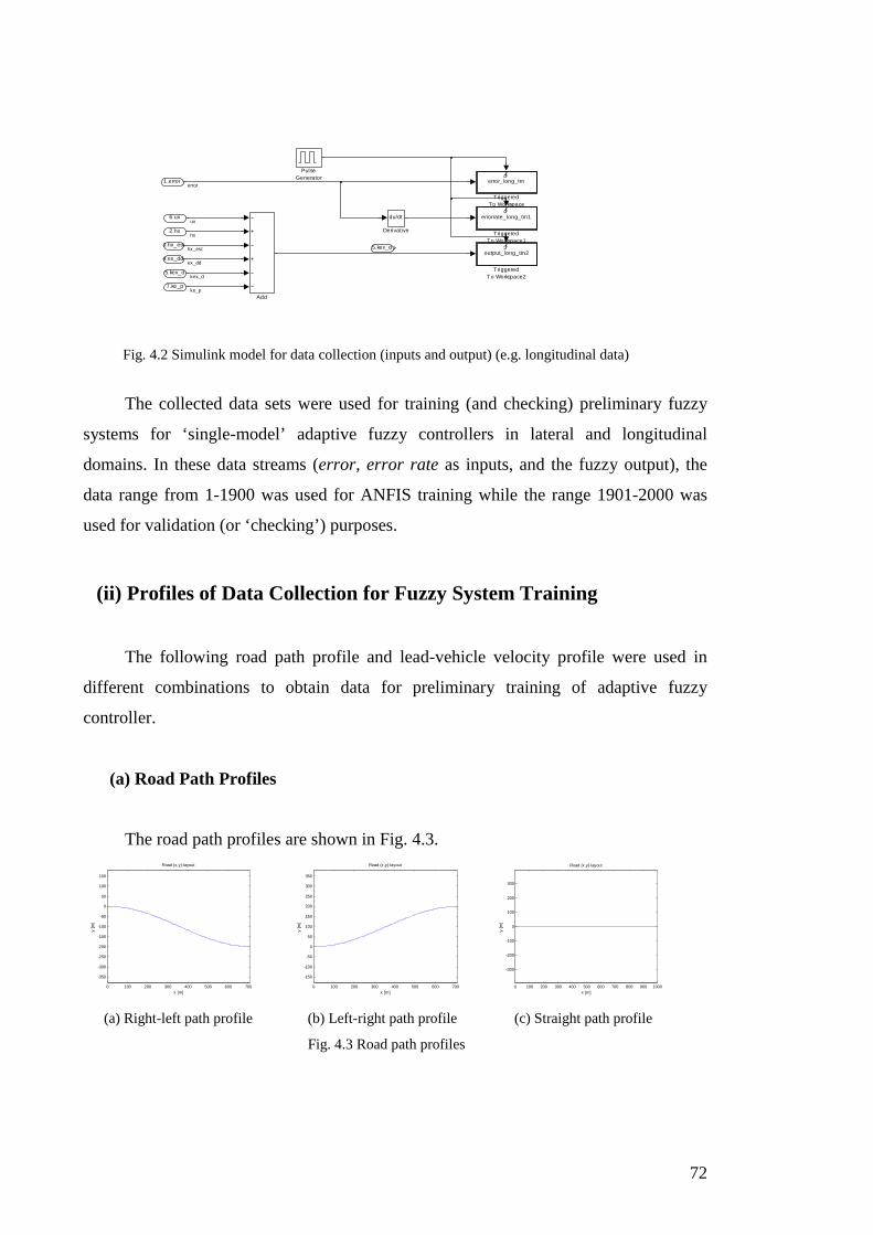
72
output_long_trn2
TriggeredTo Workspace2
errorrate_long_trn1
TriggeredTo Workspace1
error_long_trn
TriggeredTo Workspace
PulseGenerator
5.kex_d
du/dt
Derivative
Add
7.ke_p
6.ux
5.kex_d
4.ex_dd
3.hx_est
2.hx
1.errorerror
hx
kex_d
ex_dd
hx_est
ke_p
ux
Fig. 4.2 Simulink model for data collection (inputs and output) (e.g. longitudinal data)
The collected data sets were used for training (and checking) preliminary fuzzy
systems for ‘single-model’ adaptive fuzzy controllers in lateral and longitudinal
domains. In these data streams (error, error rate as inputs, and the fuzzy output), the
data range from 1-1900 was used for ANFIS training while the range 1901-2000 was
used for validation (or ‘checking’) purposes.
(ii) Profiles of Data Collection for Fuzzy System Training
The following road path profile and lead-vehicle velocity profile were used in
different combinations to obtain data for preliminary training of adaptive fuzzy
controller.
(a) Road Path Profiles
The road path profiles are shown in Fig. 4.3.
0 100 200 300 400 500 600 700
-350
-300
-250
-200
-150
-100
-50
0
50
100
150
Road (x,y)-layout
x [m]
y [m
]
0 100 200 300 400 500 600 700
-150
-100
-50
0
50
100
150
200
250
300
350
Road (x,y)-layout
x [m]
y [m
]
0 100 200 300 400 500 600 700 800 900 1000
-300
-200
-100
0
100
200
300
Road (x,y)-layout
x [m]
y [m
]
(a) Right-left path profile (b) Left-right path profile (c) Straight path profile
Fig. 4.3 Road path profiles

73
(b) Velocity Profiles (of Leading Vehicle)
The two velocity profiles of the leading vehicle used for obtaining data, are shown
in Fig. 4.4. These profiles were used in combination with the road path profiles shown
in Fig. 4.3.
0 2 4 6 8 10 12 14 16 18 200
5
10
15
20
25
time [s]
Vel
ocity
[m
/s]
(a) Constant velocity 10[m/s] and acceleration 1[m/s2]
0 2 4 6 8 10 12 14 16 18 209
9.5
10
10.5
11
time [s]
Vel
ocity
[m
/s]
(b) Constant velocity 10[m/s]
Fig. 4.4 Velocity profiles of leading vehicle
(iii) Data for Adaptive Fuzzy System Training
(a) Longitudinal Data
The following Figs. 4.5(a)–4.5(b) provide input data for longitudinal fuzzy
controller training, while Fig. 4.5(c) provides the expected output of the controller.
These data were used to train the longitudinal adaptive fuzzy controller.

74
0 200 400 600 800 1000 1200 1400 1600 1800 2000-10
-5
0
5
10
15
data number
long
itudi
nal e
rror
[m
]
(a) Longitudinal control inputs: error [m] data profile
0 200 400 600 800 1000 1200 1400 1600 1800 2000-8
-6
-4
-2
0
2
4
6
8
10
12
data number
long
itudi
nal e
rror
rat
e [m
/s]
(b) Longitudinal control input: error rate [m/s] data profile
0 200 400 600 800 1000 1200 1400 1600 1800 2000-5
-4
-3
-2
-1
0
1
2
3x 10
6
data number
long
itudi
nal o
utpu
t
(c) Longitudinal control output: data profile
Fig. 4.5 Longitudinal data profile for training
(b) Lateral Data
Similar to the longitudinal case, the following Figs. 4.6(a)–4.6(b) provide input
data for lateral fuzzy controller training, while Fig. 4.6(c) provides the expected output
of the controller. These data were used to train the lateral adaptive fuzzy controller.

75
0 200 400 600 800 1000 1200 1400 1600 1800 2000-0.05
-0.04
-0.03
-0.02
-0.01
0
0.01
0.02
0.03
0.04
0.05
data number
late
ral e
rror
[m
]
(a) Lateral control input: error [m] data profile
0 200 400 600 800 1000 1200 1400 1600 1800 2000-0.25
-0.2
-0.15
-0.1
-0.05
0
0.05
0.1
0.15
0.2
0.25
data number
late
ral e
rror
rat
e [m
/s]
(b) Lateral control input: error rate [m/s] data profile
0 200 400 600 800 1000 1200 1400 1600 1800 2000-1.5
-1
-0.5
0
0.5
1
1.5x 10
5
data number
late
ral o
utpu
t
(c) Lateral control output: data profile
Fig. 4.6 Lateral data profile for training
(iv) Classification and Clustering of Data Streams
The following identification of clusters is based on the fuzzy C-means clustering
method, and it is presented only for illustrative purposes. The fuzzy C-means clustering
was not used in the design process of the fuzzy controller in this research. Instead, the
subtractive clustering method was used to identify the clusters as well as for generating
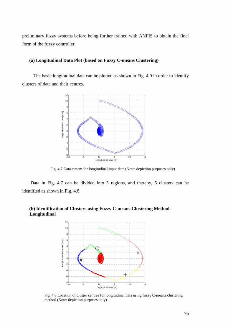
76
preliminary fuzzy systems before being further trained with ANFIS to obtain the final
form of the fuzzy controller.
(a) Longitudinal Data Plot (based on Fuzzy C-means Clustering)
The basic longitudinal data can be plotted as shown in Fig. 4.9 in order to identify
clusters of data and their centres.
-10 -5 0 5 10 15-8
-6
-4
-2
0
2
4
6
8
10
12
Longitudinal error [m]
Long
itudi
nal e
rror
rat
e [m
/s]
Fig. 4.7 Data stream for longitudinal input data (Note: depiction purposes only)
Data in Fig. 4.7 can be divided into 5 regions, and thereby, 5 clusters can be
identified as shown in Fig. 4.8.
(b) Identification of Clusters using Fuzzy C-means Clustering Method-Longitudinal
-10 -5 0 5 10 15-8
-6
-4
-2
0
2
4
6
8
10
12
Longitudinal error [m]
Long
itudi
nal e
rror
rat
e [m
/s]
Fig. 4.8 Location of cluster centres for longitudinal data using fuzzy C-means clustering method (Note: depiction purposes only)

77
The subtractive clustering method was used to generate the initial fuzzy structure,
and thereafter ANFIS method was used for fine tuning.
(c) Lateral Data Plot (based on Fuzzy C-means Clustering)
The basic lateral data can be plotted as shown in Fig. 4.9 in order to identify
clusters of data and their centres.
-0.05 -0.04 -0.03 -0.02 -0.01 0 0.01 0.02 0.03 0.04 0.05-0.25
-0.2
-0.15
-0.1
-0.05
0
0.05
0.1
0.15
0.2
0.25
Lateral error [m]
Late
ral e
rror
rat
e [m
/s]
Fig. 4.9 Data stream for lateral input data
(d) Identification of Clusters using Fuzzy C-means Clustering Method-Lateral
Data in Fig. 4.9 can be divided into 3 regions, and thereby, 3 clusters can be
identified.
-0.05 -0.04 -0.03 -0.02 -0.01 0 0.01 0.02 0.03 0.04 0.05-0.25
-0.2
-0.15
-0.1
-0.05
0
0.05
0.1
0.15
0.2
0.25
Lateral error [m]
Late
ral e
rror
rat
e [m
/s]
Fig. 4.10 Location of cluster centres for lateral data using fuzzy C-means clustering method (Note: depiction purposes only)

78
It is important to note that, in order to get good results from clustering methods,
one condition to be considered is that the data used should conform to a specific type of
distribution [93]. But, it seemed this condition was not possible to be met with above
vehicle data since they did not follow a known distribution as such. Therefore, it was
not appropriate to strictly follow the cluster centres that were produced following the
fuzzy C-means clustering method. Instead, since subtractive clustering method had an
advantage over fuzzy C-means clustering method, (because the former even generates a
basic fuzzy structure on identification of cluster centres), the subtractive clustering
method was chosen in this design process.
(v) ANFIS Training of Fuzzy Systems and Fuzzy Model Validation using Testing and Checking Data Sets
Neuro-adaptive learning in ANFIS system provides a technique for the fuzzy
system models developed to learn information about the data sets. In this ANFIS testing
method, the software system calculates best possible parameters for the fuzzy system so
that it can accurately track the given data set [173].
In the process of fuzzy model validation, input/output vectors are chosen from
collected data that has not been used to train the fuzzy system. This data is presented to
the trained fuzzy system to observe how well the system predicts on the corresponding
outputs of data sets. It is important to select a set of data that represents the data the
trained fuzzy system is intended to emulate while the selected data being sufficiently
distinct from the training data set so that the process of validation will not be trivial.
Testing or checking data is used to check the generalization capability of the
developed fuzzy system.
The objective behind validation of fuzzy models is that after a certain point in
training the model becomes over-fitting the training data set. As a principle, the model
error with checking begins to decrease up to the point the over-fitting begins. At this
point, the model error for checking starts to increase. Thereby, the fuzzy model
parameters can be chosen at the point that associates with the minimum checking error
[93].
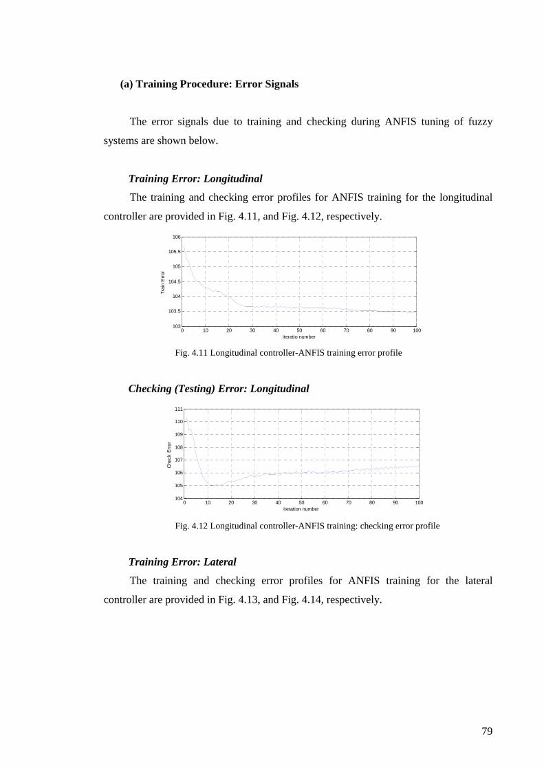
79
(a) Training Procedure: Error Signals
The error signals due to training and checking during ANFIS tuning of fuzzy
systems are shown below.
Training Error: Longitudinal
The training and checking error profiles for ANFIS training for the longitudinal
controller are provided in Fig. 4.11, and Fig. 4.12, respectively.
0 10 20 30 40 50 60 70 80 90 100103
103.5
104
104.5
105
105.5
106
iteratio number
Tra
in E
rror
Fig. 4.11 Longitudinal controller-ANFIS training error profile
Checking (Testing) Error: Longitudinal
0 10 20 30 40 50 60 70 80 90 100104
105
106
107
108
109
110
111
iteration number
Che
ck E
rror
Fig. 4.12 Longitudinal controller-ANFIS training: checking error profile
Training Error: Lateral
The training and checking error profiles for ANFIS training for the lateral
controller are provided in Fig. 4.13, and Fig. 4.14, respectively.

80
0 10 20 30 40 50 60 70 80 90 1000.125
0.13
0.135
0.14
0.145
iteration number
Tra
in E
rror
Fig. 4.13 Lateral controller-ANFIS training error profile
Checking (Testing) Error: Lateral
0 10 20 30 40 50 60 70 80 90 10034.358
34.36
34.362
34.364
34.366
34.368
34.37
34.372
34.374
iteration number
Che
ck E
rror
Fig. 4.14 Lateral controller-ANFIS training: checking error profile
(b) Longitudinal Input Fuzzy Membership Functions
Figs. 4.15–4.16 provide the input fuzzy membership functions, i.e. ‘error’ and
‘error rate’, respectively, for the longitudinal controller.
-6 -4 -2 0 2 4 6 8 10 12 14
0
0.2
0.4
0.6
0.8
1
Longitudinal error [m]
Deg
ree
of m
embe
rshi
p
largepossmallposlargeneg zerosmallneg
Fig. 4.15 Longitudinal inputs: ‘error’ fuzzy membership function
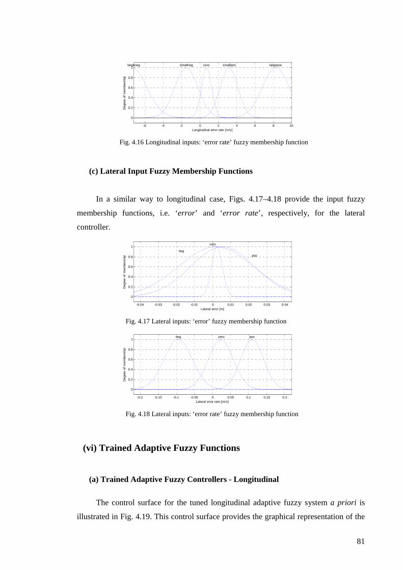
81
-6 -4 -2 0 2 4 6 8 10
0
0.2
0.4
0.6
0.8
1
Longitudinal error rate [m/s]
Deg
ree
of m
embe
rshi
p
largeposlargeneg zero smallpossmallneg
Fig. 4.16 Longitudinal inputs: ‘error rate’ fuzzy membership function
(c) Lateral Input Fuzzy Membership Functions
In a similar way to longitudinal case, Figs. 4.17–4.18 provide the input fuzzy
membership functions, i.e. ‘error’ and ‘error rate’, respectively, for the lateral
controller.
-0.04 -0.03 -0.02 -0.01 0 0.01 0.02 0.03 0.04
0
0.2
0.4
0.6
0.8
1
Lateral error [m]
Deg
ree
of m
embe
rshi
p
neg
zero
pos
Fig. 4.17 Lateral inputs: ‘error’ fuzzy membership function
-0.2 -0.15 -0.1 -0.05 0 0.05 0.1 0.15 0.2
0
0.2
0.4
0.6
0.8
1
Lateral error rate [m/s]
Deg
ree
of m
embe
rshi
p
zeroneg pos
Fig. 4.18 Lateral inputs: ‘error rate’ fuzzy membership function
(vi) Trained Adaptive Fuzzy Functions
(a) Trained Adaptive Fuzzy Controllers - Longitudinal
The control surface for the tuned longitudinal adaptive fuzzy system a priori is
illustrated in Fig. 4.19. This control surface provides the graphical representation of the

82
relationship between the two inputs, i.e., ‘error’ and ‘error rate’ and the preliminary
output of the longitudinal adaptive fuzzy system. Obvisously, this control surface is
bound to change with the adaptation process leading to a more ‘nonlinearized’ form.
-50
510
-50
510
-6
-4
-2
0
2
x 106
error rate [m/s]error [m]
outp
ut
The ANFIS tuned ‘longitudinal’ Gaussian input membership functions, i.e., for
‘error’ and ‘error rate’, as well as T–S fuzzy output membership functions a priori , are
provided in APPENDIX C.
(b) Trained Adaptive Fuzzy Controllers - Lateral
The control surface for the tuned lateral adaptive fuzzy system a priori is
illustrated in Fig. 4.20.
Fig. 4.19 Control surface for longitudinal adaptive fuzzy controller setup a priori
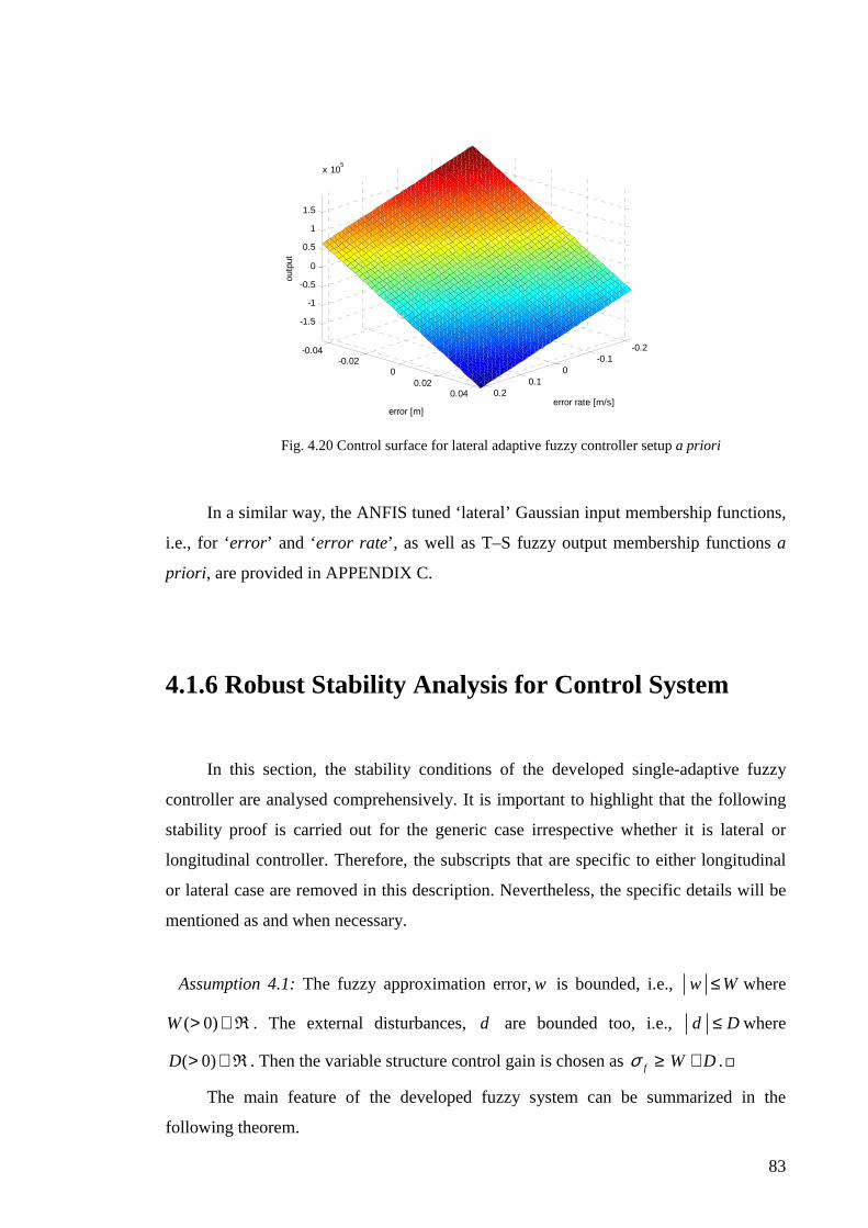
83
-0.2-0.1
00.1
0.2
-0.04-0.02
00.02
0.04
-1.5
-1
-0.5
0
0.5
1
1.5
x 105
error rate [m/s]error [m]
outp
ut
In a similar way, the ANFIS tuned ‘lateral’ Gaussian input membership functions,
i.e., for ‘error’ and ‘error rate’, as well as T–S fuzzy output membership functions a
priori , are provided in APPENDIX C.
4.1.6 Robust Stability Analysis for Control System
In this section, the stability conditions of the developed single-adaptive fuzzy
controller are analysed comprehensively. It is important to highlight that the following
stability proof is carried out for the generic case irrespective whether it is lateral or
longitudinal controller. Therefore, the subscripts that are specific to either longitudinal
or lateral case are removed in this description. Nevertheless, the specific details will be
mentioned as and when necessary.
Assumption 4.1: The fuzzy approximation error,w is bounded, i.e., w W≤ where
( 0)W > ∈R . The external disturbances, d are bounded too, i.e., d D≤ where
( 0)D > ∈R . Then the variable structure control gain is chosen as f W Dσ ≥ + .
The main feature of the developed fuzzy system can be summarized in the
following theorem.
Fig. 4.20 Control surface for lateral adaptive fuzzy controller setup a priori
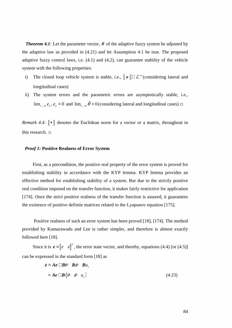
84
Theorem 4.1: Let the parameter vector, θ of the adaptive fuzzy system be adjusted by
the adaptive law as provided in (4.21) and let Assumption 4.1 be true. The proposed
adaptive fuzzy control laws, i.e. (4.1) and (4.2), can guarantee stability of the vehicle
system with the following properties:
i) The closed loop vehicle system is stable, i.e., ∈e ∞L (considering lateral and
longitudinal cases)
ii) The system errors and the parametric errors are asymptotically stable, i.e.,
lim 0t x ye , e→∞ = and lim 0t θ→∞ =ɶ (considering lateral and longitudinal cases).
Remark 4.4: • denotes the Euclidean norm for a vector or a matrix, throughout in
this research.
Proof 1: Positive Realness of Error System
First, as a precondition, the positive real property of the error system is proved for
establishing stability in accordance with the KYP lemma. KYP lemma provides an
effective method for establishing stability of a system. But due to the strictly positive
real condition imposed on the transfer function, it makes fairly restrictive for application
[174]. Once the strict positive realness of the transfer function is assured, it guarantees
the existence of positive definite matrices related to the Lyapunov equation [175].
Positive realness of such an error system has been proved [18], [174]. The method
provided by Kumarawadu and Lee is rather simpler, and therefore is almost exactly
followed here [18].
Since it is [ ] ,T
e e=e ɺ the error state vector, and thereby, equations (4.4) [or (4.5)]
can be expressed in the standard form [18] as
sd uν= + − −e Ae B B Bɺ ɶ
( )sd uν= + − −Ae B ɶ (4.23)

85
where 0 1
p dk k
= − −
A , and 0
1
=
B . A number of such error models have been
comprehensively analysed [163]. The output error signal of the error dynamic system
can be expressed as
R e e= = +Ce ɺ , (4.24)
since it is earlier provided that [ ]1 1=C . The equations (4.23) and (4.24) describe the
state-space representation of the error dynamics. When 1dk ≥ , and 0pk ≥ the real part
of the transfer function 1( ) ( ) / ( ) ( )G s R s s sν −= = −C I A Bɶ ( s is the Laplace operator),
i.e. Re ( )G s ϑ− , is positive for 0ϑ > where ϑ ∈R , if
2 2
2 2
( 1)( ) ( 1).
( )d d p
p d
k k k
k k
σ ϑ ωσ ϑ
σ ϑ ω + − + − +
− > − − + + + (4.25)
This implies that ( )G s ϑ− is positive real for 0ϑ > , and consequently ( )G s is strictly
positive real [175], [176]. The re-verification of the positive-real property of the above
transfer function can be done by drawing a Nyquist diagram with the chosen values of
dk and pk [174].
Proof 2: System Stability
According to Kalman–Yakubovich–Popov (KYP) lemma [175], for a strictly
positive real system, there exist two positive definite matrices P and Q
(i.e., 0T= >P P and 0T= >Q Q ) satisfying
T + + =A P PA Q 0, and T=PB C . (4.26)
Now, the following Lyapunov function can be defined as (for lateral or longitudinal
system)
1TVγ
= + Te Pe θ θɶ ɶ (4.27)
where 0γ > is a real constant, and *= −θ θ θɶ is the parameter error with respect
to the optimal parameter set. Here, * 2n×∈θ R where n is the total number of fuzzy rules,
is the optimal parameter vector of the adaptive fuzzy controller.

86
The Lyapunov candidate, as provided in (4.27) quantifies both in tracking error
and in parameter estimates. Differentiating the Lyapunov function along the trajectories
of the error system will provide
1( ) ( )T T TV γ= + + + Te Pe e Pe θ θ θ θɺ ɺɶ ɶ ɶ ɶɺ ɺ ɺ . (4.28)
Substituting for eɺ from the equation (4.23), in (4.28) provides
( )( ) ( )( )1 ( ).
T Ts sV d u d u
γ
ν ν= + − − + + − −
+ T T
Ae B Pe e P Ae B
θ θ + θ θ
ɺ ɶ ɶ
ɺ ɺɶ ɶ ɶ ɶ
Further rearrangement will provide
( ) ( )( )TT T T T
s sV d u d uν ν= + + − − + − −e A P PA e B Pe e PBɺ ɶ ɶ (4.29)
1 ( ).γ+ T Tθ θ + θ θɺ ɺɶ ɶ ɶ ɶ
From the argument, it can be expressed as
( )* ˆ ( )( ) ( )T Tw x w x wν ν ν= − + = − + = +*θ θ θɶɶ ξ ξ where w is the fuzzy approximation
error which is bounded,w W≤ , i.e.,w ∞∈L , and W ∈R is a positive constant. The
determination of fuzzy approximation error upper bound, W has been discussed before
[30].
Hence, (4.29) becomes
( )( ) 1
( )
( ) ( ).
T Ts
T Ts
V x w d u
x w d u γ
= − + + − −
+ + − − +
ɶɺ
ɺ ɺɶ ɶ ɶ ɶ ɶ
T
T T
e Qe θ B Pe
e PB θ θ θ + θ θ
ξ
ξ (4.30)
Rearranging (4.30) provides
( ) ( )( )( )
1 1( ) ( )
.
TT
T Ts
V x x
w d u
γ γ= − + + + +
+ − − +
Te Qe θ θ Ce θ Ce θ
Ce e C
ɺ ɺɶ ɶ ɶ ɶɺ ξ ξ (4.31)
If the fuzzy adaptive law is taken as ( )xγ= −θ Ceɺ ξ as provided in (4.21), with
( ) 0γ ∈ >R as the adaptive parameter, (4.31) reduces to
( )( )T T TsV w d u= − + − − +e Qe Ce e Cɺ . (4.32)
The equation (4.32) can be further expressed as
( )( )2
min .T TsV w d uλ≤ − + − − +Q e Ce e Cɺ (4.33)
Here, minλQ is the minimum eigen value of Q .

87
Since fuzzy systems follow universal approximation theorem [29], w may be
made arbitrarily small by a proper choice of the fuzzy system if ( )T xν = θξ is smooth
(note that this may require an arbitrarily large number of rules) [30].
Since w W≤ and d D≤ , (4.33) can be further written as
( )( )2
minT T
sV W D uλ≤ − + + − +Q e Ce e Cɺ . (4.34)
Let the variable structure control term be defined as
( )sign T Ts fu σ= +Ce e C . (4.35)
Thereby, (4.34) can be expressed as
( )2
minT T
fV W Dλ σ≤ − + + − +Q e Ce e Cɺ . (4.36)
Further rearrangement of (4.36) will provide
( )2
minT T
fV W Dλ σ≤ − − + − −Q e Ce e Cɺ . (4.37)
If it is taken as
f W Dσ ≥ + , (4.38)
then (4.37) will establish that
0V ≤ɺ , 0t∀ ≥ . (4.39)
Therefore, according to Lyapunov theory, it establishes the fact that e is bounded,
i.e. ∞∈e L . Therefore, ,e eɺ are bounded, too, i.e. ,e e ∞∈ɺ L . It also establishes that
parameter errors are bounded, i.e., ∞∈θɶ L .
Equation (4.37) also implies that
2
minV λ≤ − Q eɺ . (4.40)
Integrating (4.40) will provide
2
min 0 0(0) ( )dt Vdt V Vλ
∞ ∞≤ − = − ∞∫ ∫Q e ɺ . (4.41)
Therefore, rearranging (4.41) will provide
( )min
2 1
0(0) ( )dt V Vλ
∞≤ − ∞∫ Q
e . (4.42)

88
Equation (4.42) establishes that
2∈e L 2 2
0( ) : ( )z t z t dt
∞ = < ∞ ∫L , (4.43)
since it provides (0), ( )V V ∞∞ ∈L according to (4.39) [30]. Since it has been obtained
2e ∞∈L L∩ (from (4.43) and (4.39)), and e ∞∈ɺ L (from (4.40)), by Barbalat’s lemma
[30], [176], it can be established with asymptotic stability of e (i.e. lim 0t e→∞ = ). This
result of asymptotic stability can be extended specifically to lateral and longitudinal
cases, and consequently the lateral and longitudinal errors are asymptotically stable, i.e.
lim 0.t x ye , e→∞ = (4.44)
The equation (4.44) proves that when lateral and longitudinal cases are considered
at the same time, with the above arguments, the system of errors can be proved
asymptotically stable. Therefore, the result provided in (4.44) logically proves that the
integrated lateral and longitudinal control system is asymptotically stable. This
statement completes the proof of stability for robust single-adaptive fuzzy system.
The following definition is provided to formerly identify the variable vector
spaces, and thereby to define the optimal parameter set.
Definition 4.1: The compact parameter spaces for θ and x variables can be defined as
below. Let ( 0)Mθ > ∈R and ( 0)xM > ∈R be finite
: Mθ = ∈ ≤θ
Ω θ θR , and
:x xx x M= ∈ ≤Ω R .
Thereby, the optimal parameter set can be formally defined as
*arg min sup ( )x
T
x
xθ
ν∗
∈ ∈
= − θ Ω Ω
θ θξ (4.45)
where * ( )ν ∈R is the optimal adaptive fuzzy function output.
Remark 4.5: The usage of the term *θ is only for analytical purposes in this proof. The
value of it is not required in the design of the controller.
Remark 4.6 [176]: The above Lyapunov candidate (4.27) satisfies the following
conditions
i) V is at least 1C

89
ii) (0) 0V = and ( ( )) 0V x t > for ( ) 0x t ≠ , and
iii) ( )x t → ∞ ⇒ ( ( ))V x t → ∞
( ( )x t denotes a selected time-dependent state of the system in this remark).
Remark 4.7: An update law with a projection operator can be defined to guarantee that
the parameter matrices lie within the feasible parametric space. Details on using a
projection operator were provided in [30], [32], and the references, therein. It is also
important to note that the requirement of a projection operator is only to establish
stability in the theoretical sense.
4.1.7 Simulation Studies, Results and Discussion
The following simulations were done on veDYNA® (ver. 3.10) vehicle
simulation software with a BMW 325i 1988 model. The simulation setup consists of
front wheel-steered, front wheel-driven, automatic transmission settings. veDYNA®
runs with an ordinary differential solver ‘ode1’ based on trapezoidal method with a
sample time 0.001 [s]. But the developed controller and the inverse model were run
with a solver ‘ode4’ viz. a 4-th order Runge-Kutta method, and with a sample time
0.0005 [s]. This new setting for the controller and inverse model was adopted because
the embedded fuzzy systems looked ‘stiff’ with integration with a simpler differential
solver of calibre ‘ode1’. In order to overcome this difficult issue, veDYNA® vehicle
model was encapsulated in a triggered subsystem on Simulink/ MATLAB®, as shown
in Fig. 3.10, and thereby, was connected to the external control system. Hence,
MATLAB® ordinary differential equation command ‘ode4’was used with the fixed step
size 0.0005 [s] for all vehicle controller modules.
While the simulation studies were aimed for solving the integrated lateral and
longitudinal control problem of highway vehicles, the viability of the controller was
also tested under simulated extreme parametric changes: changing of friction coefficient
of tyre-road interface, presence of disturbances like crosswind forces, addition of an
unsymmetrical external load. These disturbances were used to challenge the robust
setting of the control system. Additionally, the performance of the developed controller
was tested against some occurrences of faulty conditions at selected subsystems at non-
catastrophic level. The considered faulty conditions included a flat-tyre case (front-left

90
tyre becoming flat at 10[s] after starting the simulation), and a defective front-left wheel
brake cylinder (with a 90% pressure drop in the supply line, throughout).
(i) Simulation Setup
The PD gains for the controller were chosen as follows: for the longitudinal case;
1e5pxk = , 1e5dxk = , and for the lateral case; 1e6pyk = , 1e5dyk = .
The adaptive gains in the fuzzy controllers were chosen as 0.03xγ = and
0.01yγ = for longitudinal and lateral cases, respectively. And the gains for variable
structure control terms were taken as 275fxσ = and 225fyσ = for longitudinal and
lateral cases, respectively.
The inter-vehicular gap was taken as a constant value of 5 [m], for simplicity. The
simulation profile used is shown in Figs. 4.21–4.23 below. The speed of the leading
vehicle is varying from 0 [m/s] to 35 [m/s] with a maximum longitudinal
acceleration/deceleration of ± 1.5 [m/ 2s ], a value within the realistic capacity of vehicle
operation [14].
As provided in Fig. 4.22, the radii of curvature of the highway path varies
between [0 315] [m]. It is important to note that the controlled vehicle starts from zero
velocity. This is important to testify the controller performance with more pronounced
transient effects. In the meanwhile the leading vehicle cruises right on the highway
centreline throughout.
(ii) Simulation Profile
The following figures, Figs. 4.21–4.23 describe the simulation profile used for
validation of all the controllers developed in this research.
(a) Road Profile
The road path that was used in the simulation on veDYNA® is shown in Fig.
4.21. This road path consists of straight line segments as well as cubic-splines.

91
0 500 1000 1500
-400
-200
0
200
400
600
800
Road (x,y)-layout
x-coordinate [m]y-
coor
dina
te [
m]
Fig. 4.21 Road profile
(b) Radii of Curvature Variation of the Road
Fig. 4.22 shows the curvature of the road profile provided in Fig. 4.21.
0 200 400 600 800 1000 1200 1400 1600 1800 2000-4
-3
-2
-1
0
1
2
3
4x 10
-3 Road curvature
Road Length [m]
Cur
vatu
re [
1/m
]
Fig. 4.22 Radii of curvature along the road
(c) Lead Vehicle Velocity Profile
The velocity profile of the lead vehicle is illustrated in Fig. 4.23. For comparison
purposes, the controlled vehicle velocities with adaptive fuzzy controller at on and off
(PD only) states are also provided.
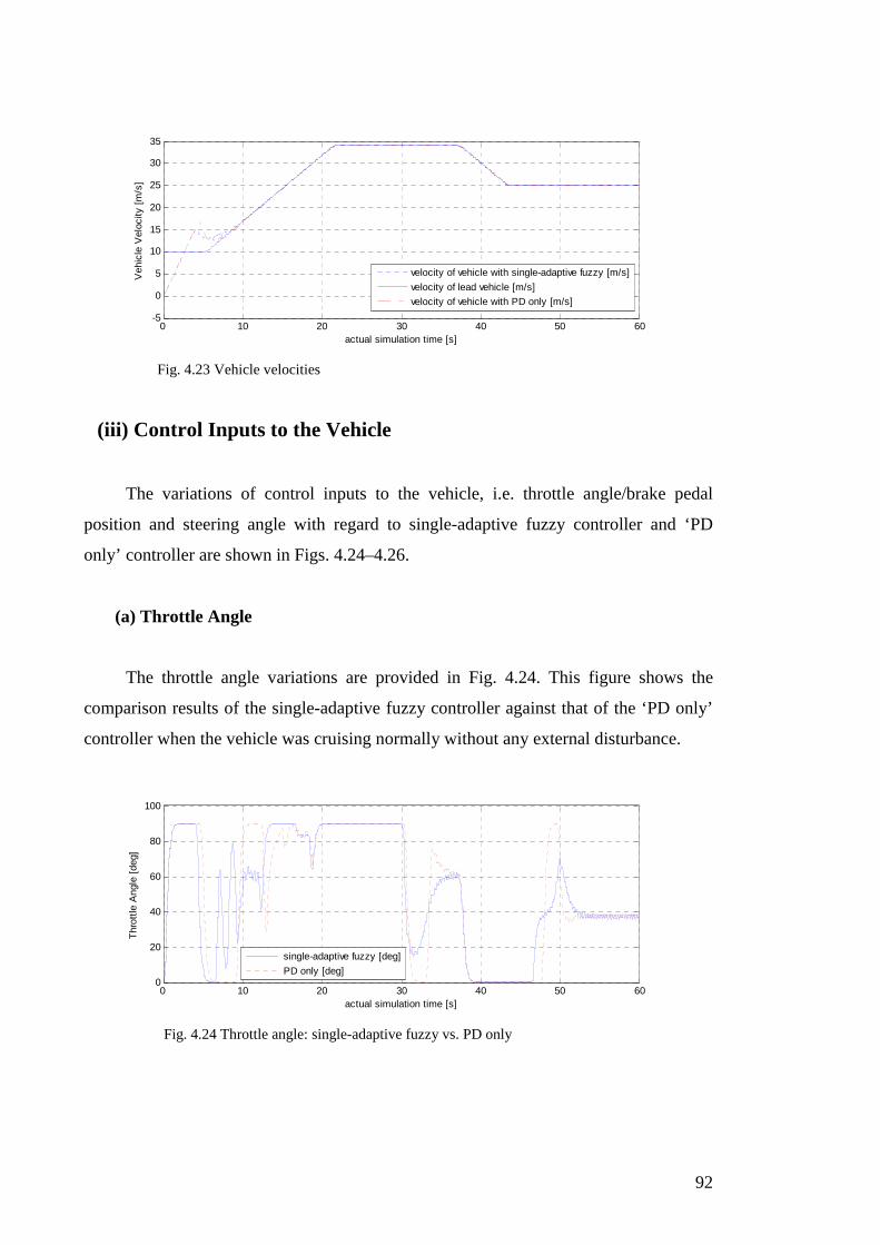
92
0 10 20 30 40 50 60-5
0
5
10
15
20
25
30
35
actual simulation time [s]
Veh
icle
Vel
ocity
[m
/s]
velocity of vehicle with single-adaptive fuzzy [m/s]
velocity of lead vehicle [m/s]
velocity of vehicle with PD only [m/s]
Fig. 4.23 Vehicle velocities
(iii) Control Inputs to the Vehicle
The variations of control inputs to the vehicle, i.e. throttle angle/brake pedal
position and steering angle with regard to single-adaptive fuzzy controller and ‘PD
only’ controller are shown in Figs. 4.24–4.26.
(a) Throttle Angle
The throttle angle variations are provided in Fig. 4.24. This figure shows the
comparison results of the single-adaptive fuzzy controller against that of the ‘PD only’
controller when the vehicle was cruising normally without any external disturbance.
0 10 20 30 40 50 600
20
40
60
80
100
actual simulation time [s]
Thr
ottle
Ang
le [
deg]
single-adaptive fuzzy [deg]
PD only [deg]
Fig. 4.24 Throttle angle: single-adaptive fuzzy vs. PD only

93
(b) Brake Pedal Position
The brake pedal position variations are depicted in Fig. 4.25. In comparison with
Fig. 4.24, which provides the variation of throttle angle, it is clear that when the brake
pedal position becomes positive, the throttle angle stays at zero level.
0 10 20 30 40 50 600
20
40
60
80
100
actual simulation time [s]
Bra
ke P
edal
Pos
ition
[%
]
PD only
Single-adaptive fuzzy
Fig. 4.25 Brake pedal position: single-adaptive fuzzy vs. PD only
(c) Steering Angle
Fig. 4.26 provides the steering angle variation. In a similar way as before, this
figure compares steering angle from single-adaptive fuzzy controller with that from ‘PD
only’ controller when the vehicle was cruising normally without any external
disturbances.
0 10 20 30 40 50 60-0.01
-0.005
0
0.005
0.01
0.015
0.02
0.025
actual simulation time [s]
Ste
erin
g A
ngle
[ra
d]
steering angle withsingle-adaptive fuzzy [rad]
steering angle withoutsingle-adaptive fuzzy [rad]
Fig. 4.26 Steering angle: single-adaptive fuzzy vs. ‘PD only’

94
(d) Vehicle Lateral Position
Fig. 4.27 provides the lateral deviation of the vehicle centre of gravity in global
coordinates. This figure is mainly provided for comparison purposes with the other
graphs for the movement of the vehicle.
0 10 20 30 40 50 600
100
200
300
400
500
actual simulation time [s]
Late
ral P
ositi
on o
f V
ehic
le C
.G.
[m]
Fig. 4.27 Lateral position of vehicle centre of gravity
(iv) Simulation Results and Discussion
In the following figures depicting simulation results, each performance parameter
of single-adaptive fuzzy controller (solid blue line) is compared against that of ‘PD
only’ controller (dotted red line).
(a) Normal Cruising Conditions: Single-Adaptive Fuzzy Control
The following simulation results provide the performance of the developed single-
adaptive fuzzy controller against that of the ‘PD only’ controller under normal cruising
conditions without any presence of external disturbances.
As shown in Fig. 4.28, there is hardly any improvement of longitudinal error of
adaptive fuzzy over ‘PD only’ controller. It can be said that the change is slightly worse
when it comes to response time initially, i.e. around the points 5–9 [s] on the time-scale.
Therefore, ‘PD only’ controller is quite effective when compared to the single-adaptive
fuzzy controller as far as longitudinal control is concerned in this case.

95
0 10 20 30 40 50 60-2
0
2
4
6
8
10
12
14
actual simulation time [s]
Long
itudi
nal e
rror
[m
]
longitudinal error with adaptive fuzzy
longitudinal error without adaptive fuzzy
Fig. 4.28 Longitudinal error: single-adaptive fuzzy (RMS: 3.158) vs. ‘PD only’ (RMS: 3.078)
Fig. 4.29 shows that the lateral error has improved significantly with adaptive
fuzzy controller over ‘PD only’ controller. Therefore, it can be concluded that the
single-adaptive fuzzy controller contributes significantly to improve the lateral tracking
of the vehicle under normal cruising.
0 10 20 30 40 50 60-0.06
-0.04
-0.02
0
0.02
0.04
0.06
actual simulation time [s]
Late
ral e
rror
[m
]
lateral error without adaptive fuzzy
lateral error with adaptive fuzzy
Fig. 4.29 Lateral error: single-adaptive fuzzy (RMS: 0.003837) vs. ‘PD only’ (RMS: 0.01849)
The pitch angle variation due to the single-adaptive fuzzy controller is comparable
to that with the ‘PD only’ controller as shown in Fig. 4.30. At some points, adaptive
fuzzy controller has avoided reaching some ‘extreme’ values, e.g. around 5 [s] on the
time-scale. It concludes that pitch angle variation effects are quite small, since the range
of vertical movement of the suspension mass just above the front axle lies within [-0.03
0.02] [rad], which is similar to an approximate range of 3 [deg] variation. This is
equivalent to approximately 4 [cm] maximum deviation from the normal level of the
suspension mass just above the front axle through the longitudinal axis.

96
0 10 20 30 40 50 60-0.04
-0.03
-0.02
-0.01
0
0.01
0.02
0.03
0.04
actual simulation time [s]
Pitc
h A
ngle
[ra
d]
pitch angle without adaptive fuzzy [rad]
pitch angle with adaptive fuzzy [rad]
Fig. 4.30 Pitch angle: single-adaptive fuzzy (RMS: 0.01195) vs. ‘PD only’ (RMS: 0.01202)
Roll angle, as shown in Fig. 4.31, exhibits some slight improvements with
transient response with the adaptive fuzzy controller. These effects are most evidenced
around the points 15 [s], and 45–47 [s], on the time-scale. Roll angle gives an indication
of lateral stability of the vehicle.
0 10 20 30 40 50 60-0.025
-0.02
-0.015
-0.01
-0.005
0
0.005
0.01
0.015
0.02
0.025
actual simulation time [s]
Rol
l Ang
le [
rad]
roll angle with adaptive fuzzy [rad]
roll angle without adaptive fuzzy [rad]
Fig. 4.31 Roll angle: single-adaptive fuzzy (RMS: 0.01086) vs. ‘PD only’ (RMS: 0.01094)
Roll rate is another indication of lateral stability of the vehicle. As shown in Fig.
4.32, adaptive fuzzy controller performance is comparable to that of the ‘PD only’
controller as far as roll rate is concerned.
0 10 20 30 40 50 60-0.1
-0.05
0
0.05
0.1
0.15
actual simulation time [s]
Rol
l Rat
e [r
ad/s
]
roll rate with adaptive fuzzy [rad/s]
roll rate without adaptive fuzzy [rad/s]
Fig. 4.32 Roll rate: single-adaptive fuzzy (RMS: 0.01) vs. ‘PD only’ (RMS: 0.01171)

97
There are improvements in the transients with adaptive fuzzy controller over ‘PD
only’ controller when it comes to side-slip angle, as shown in Fig. 4.33, when the
vehicle makes a sudden change due to curvature of the road. Ensuring a low side-slip
angle, especially during transient stages makes the vehicle more stable in the lateral
context. In general case, under normal driving conditions with ensured safety, without
any danger of losing road grip, the slide-slip angle for a car does not exceed± 2 [deg]
[177]. The two controllers have performed well within this requirement of side-slip
angle.
0 10 20 30 40 50 60-0.015
-0.01
-0.005
0
0.005
0.01
0.015
0.02
actual simulation time [s]
Sid
e-S
lip A
ngle
[ra
d]
side-slip angle with adaptive fuzzy [rad]
side-slip angle without adaptive fuzzy [rad]
Fig. 4.33 Side-slip angle: single-adaptive fuzzy (RMS: 0.007206) vs. ‘PD only’ (RMS: 0.007256)
Since adaptive fuzzy controller has improved side-slip angle and roll angle
responses while maintaining the roll rate at a competitive level, it can be said that the
lateral stability of the vehicle has been improved by adaptive fuzzy controller.
The comfortable or low ranges of lateral accelerations can be categorized into
different ranges: small-signal range, i.e., 0–0.5 [m/s2] where only straight-running
behaviour can be included or ‘linear range’, i.e., 0.5–4 [m/s2] where sudden steering
inputs, lane changes and load change reaction in turns [178]. As shown in Fig. 4.34, the
variations of lateral acceleration do not go beyond 4 [m/s2]. Therefore, the two
controllers have managed to contain lateral acceleration within low limits as far as
design characteristics of today’s passenger vehicles are concerned [178].

98
0 10 20 30 40 50 60-4
-3
-2
-1
0
1
2
3
actual simulation time [s]
Late
ral A
ccel
erat
ion
[m/s
-2]
lateral acceleration with adaptive fuzzy [m/s-2]
lateral acceleration without adaptive fuzzy [m/s-2]
Fig. 4.34 Lateral acceleration: single-adaptive fuzzy (RMS: 1.264) vs. ‘PD only’ (RMS: 1.271)
In minimizing lateral acceleration, adaptive fuzzy controller has been quite
competitive with the ‘PD only’ controller, and the former has even managed to avoid
some transient effects that were present with the ‘PD only’ controller.
With comparison of side-slip angle and lateral acceleration, as shown in Figs.
4.33–4.34, the side-slip angle indicates an increase as the lateral acceleration curve
increases (disregarding the ‘sign’). This fact is an indication of controllability of the
vehicle provided that there have been less fluctuations in side-slip angle [178]. This is
quite the case with the side-slip angle performance.
Overall, during normal cruising, lateral stability with adaptive fuzzy controller is
quite competitive in comparison to the ‘PD only’ controller as suggested by the
performances in the areas of side-slip angle, roll-angle and roll rate. Therefore, having a
lower lateral tracking error is a significant result by the adaptive fuzzy controller in
comparison to the ‘PD only’ controller, with a guaranteed lateral stability. Unlike lateral
tracking, longitudinal tracking variation has not been better than that of ‘PD only’
controller.
(b) External Disturbances: Single-Adaptive Fuzzy Control
In the following set of simulations, the developed single-adaptive fuzzy controller
was tested against the ‘PD only’ controller under a number of external disturbances.
These disturbances included an unsymmetrical load mass, presence of crosswind forces
and change of tyre-road friction.

99
1. Unsymmetrical Load Mass
The following simulation was carried out for comparison of the performances
between the single-adaptive fuzzy controller and the ‘PD only’ controller, when there
was an unsymmetrical load-mass on the vehicle as per the details described in Section
3.2.18.
As shown in Fig. 4.35, the longitudinal error has slightly decreased with adaptive
fuzzy functions. Initially it has a longer response time towards the point 10 [s]. The
second peak of the curves, around 23 [s] on the time-scale, is due to sudden change in
the curvature of the road path. This response has been heightened due to an unbalanced
force that is generated in the vehicle due to unsymmetrical loading.
0 10 20 30 40 50 60-5
0
5
10
15
20
actual simulation time [s]
Long
itudi
nal E
rror
[m
]
longitudinal error with adaptive fuzzy [m]
longitudinal error without adaptive fuzzy [m]
Fig. 4.35 Longitudinal error: single-adaptive fuzzy (RMS: 4.391) vs. ‘PD only’ (RMS: 4.375)
As shown in Fig. 4.36, even in the presence of an unsymmetrical mass, the lateral
tracking has shown an improvement with adaptive fuzzy controller as against that of the
‘PD only’ controller.
0 10 20 30 40 50 60-0.06
-0.04
-0.02
0
0.02
0.04
0.06
0.08
actual simulation time [s]
Late
ral E
rror
[m
]
lateral error without adaptive fuzzy [m]
lateral error with adaptive fuzzy [m]
Fig. 4.36 Lateral error: single-adaptive fuzzy (RMS: 0.003957) vs. ‘PD only’ (RMS: 0.01741)
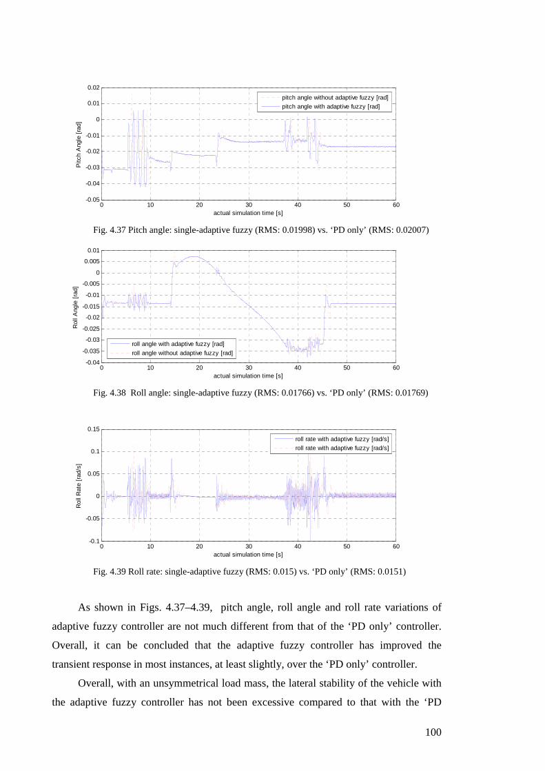
100
0 10 20 30 40 50 60-0.05
-0.04
-0.03
-0.02
-0.01
0
0.01
0.02
actual simulation time [s]
Pitc
h A
ngle
[ra
d]
pitch angle without adaptive fuzzy [rad]
pitch angle with adaptive fuzzy [rad]
Fig. 4.37 Pitch angle: single-adaptive fuzzy (RMS: 0.01998) vs. ‘PD only’ (RMS: 0.02007)
0 10 20 30 40 50 60-0.04
-0.035
-0.03
-0.025
-0.02
-0.015
-0.01
-0.005
0
0.005
0.01
actual simulation time [s]
Rol
l Ang
le [
rad]
roll angle with adaptive fuzzy [rad]
roll angle without adaptive fuzzy [rad]
Fig. 4.38 Roll angle: single-adaptive fuzzy (RMS: 0.01766) vs. ‘PD only’ (RMS: 0.01769)
0 10 20 30 40 50 60-0.1
-0.05
0
0.05
0.1
0.15
actual simulation time [s]
Rol
l Rat
e [r
ad/s
]
roll rate with adaptive fuzzy [rad/s]
roll rate with adaptive fuzzy [rad/s]
Fig. 4.39 Roll rate: single-adaptive fuzzy (RMS: 0.015) vs. ‘PD only’ (RMS: 0.0151)
As shown in Figs. 4.37–4.39, pitch angle, roll angle and roll rate variations of
adaptive fuzzy controller are not much different from that of the ‘PD only’ controller.
Overall, it can be concluded that the adaptive fuzzy controller has improved the
transient response in most instances, at least slightly, over the ‘PD only’ controller.
Overall, with an unsymmetrical load mass, the lateral stability of the vehicle with
the adaptive fuzzy controller has not been excessive compared to that with the ‘PD

101
only’ controller. This can be concluded from the performances in the areas of side-slip
angle, roll-angle and roll rate.
Side-slip angle is high with adaptive fuzzy when the speed of the vehicle is low.
This is shown in Fig. 4.40. A slack of controllability initially would be the reason for
such a display when the adaptive fuzzy controller was active [178]. In this instance,
however, adaptive fuzzy controller has not been successful in eliminating the higher
side-slip angle at low speed. But, this was only when the vehicle speed was very low.
As the vehicle gathers speed adaptive fuzzy exhibits a comparatively improved response
even with eliminating transient effects, over ‘PD only’ controller.
0 10 20 30 40 50 60-0.04
-0.03
-0.02
-0.01
0
0.01
0.02
actual simulation time [s]
Sid
e S
lip A
ngle
[ra
d]
side slip angle without adaptive fuzzy [rad]
side slip angle with adaptive fuzzy [rad]
Fig. 4.40 Side-slip angle: single-adaptive fuzzy (RMS: 0.008237) vs. ‘PD only’ (RMS: 0.008256)
As shown in Fig. 4.41, the variations in lateral acceleration do not go beyond 4
[m/s2]. Therefore, the two controllers have managed to contain the lateral acceleration
within low limits according to the design characteristics of today’s passenger vehicles
[178].
0 10 20 30 40 50 60-3
-2
-1
0
1
2
3
actual simulation time [s]
Late
ral A
ccel
erat
ion
[m/s
-2]
lateral acceleration with adaptive fuzzy [m/s-2]
lateral acceleration without adaptive fuzzy [m/s-2]
Fig. 4.41 Lateral acceleration: single-adaptive fuzzy (RMS: 1.256) vs. ‘PD only’ (RMS: 1.262)
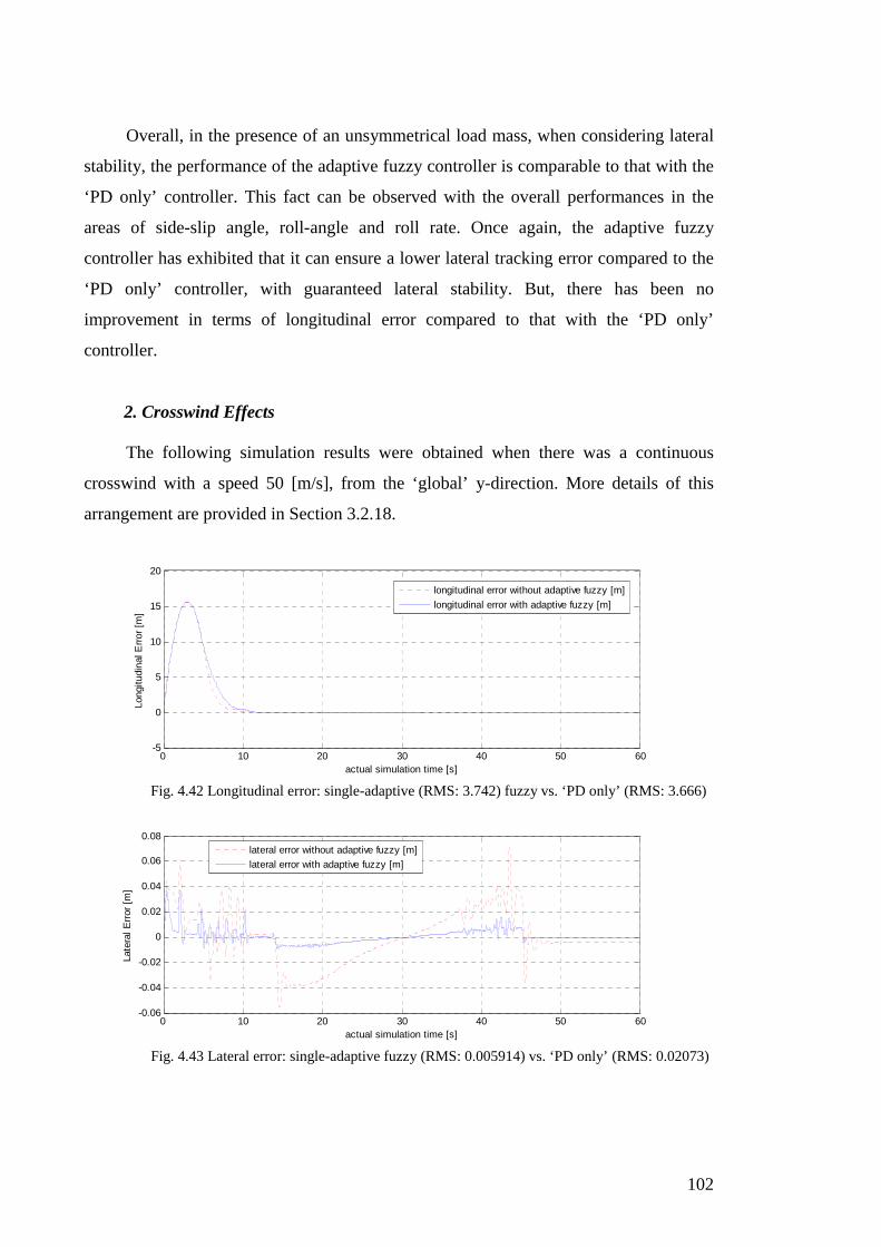
102
Overall, in the presence of an unsymmetrical load mass, when considering lateral
stability, the performance of the adaptive fuzzy controller is comparable to that with the
‘PD only’ controller. This fact can be observed with the overall performances in the
areas of side-slip angle, roll-angle and roll rate. Once again, the adaptive fuzzy
controller has exhibited that it can ensure a lower lateral tracking error compared to the
‘PD only’ controller, with guaranteed lateral stability. But, there has been no
improvement in terms of longitudinal error compared to that with the ‘PD only’
controller.
2. Crosswind Effects
The following simulation results were obtained when there was a continuous
crosswind with a speed 50 [m/s], from the ‘global’ y-direction. More details of this
arrangement are provided in Section 3.2.18.
0 10 20 30 40 50 60-5
0
5
10
15
20
actual simulation time [s]
Long
itudi
nal E
rror
[m
]
longitudinal error without adaptive fuzzy [m]
longitudinal error with adaptive fuzzy [m]
Fig. 4.42 Longitudinal error: single-adaptive (RMS: 3.742) fuzzy vs. ‘PD only’ (RMS: 3.666)
0 10 20 30 40 50 60-0.06
-0.04
-0.02
0
0.02
0.04
0.06
0.08
actual simulation time [s]
Late
ral E
rror
[m
]
lateral error without adaptive fuzzy [m]
lateral error with adaptive fuzzy [m]
Fig. 4.43 Lateral error: single-adaptive fuzzy (RMS: 0.005914) vs. ‘PD only’ (RMS: 0.02073)

103
0 10 20 30 40 50 60-0.04
-0.03
-0.02
-0.01
0
0.01
0.02
0.03
0.04
actual simulation time [s]
Pitc
h A
ngle
[ra
d]
pitch angle without adaptive fuzzy [rad]
pitch angle with adaptive fuzzy [rad]
Fig. 4.44 Pitch angle: single-adaptive fuzzy (RMS: 0.01142) vs. ‘PD only’ (RMS: 0.01146)
0 10 20 30 40 50 60-0.04
-0.03
-0.02
-0.01
0
0.01
0.02
actual simulation time [s]
Rol
l Ang
le [
rad]
roll angle with adaptive fuzzy[rad]
roll angle without adaptive fuzzy[rad]
Fig. 4.45 Roll angle: single-adaptive fuzzy (RMS: 0.01396) vs. ‘PD only’ (RMS: 0.01406)
0 10 20 30 40 50 60-0.25
-0.2
-0.15
-0.1
-0.05
0
0.05
0.1
0.15
0.2
0.25
actual simulation time [s]
Rol
l Rat
e [r
ad/s
]
roll rate with adaptive fuzzy[rad/s]
roll rate without adaptive fuzzy[rad/s]
Fig. 4.46 Roll rate: single-adaptive fuzzy (RMS: 0.02222) vs. ‘PD only’ (RMS: 0.02317)

104
0 10 20 30 40 50 60-0.02
-0.01
0
0.01
0.02
0.03
0.04
actual simulation time [s]
Sid
e S
lip A
ngle
[ra
d]
side slip angle without adaptive fuzzy [rad]
side slip angle with adaptive fuzzy [rad]
Fig. 4.47 Side-slip angle: single-adaptive fuzzy (RMS: 0.01438) vs. ‘PD only’ (RMS: 0.1475)
0 10 20 30 40 50 60-4
-3
-2
-1
0
1
2
3
actual simulation time [s]
Late
ral A
ccel
erat
ion
[m/s
2 ]
lateral acceleration with adaptive fuzzy [m/s 2]
lateral acceleration without adaptive fuzzy [m/s 2]
Fig. 4.48 Lateral acceleration: single-adaptive fuzzy (RMS: 1.285) vs. ‘PD only’ (RMS: 1.299)
Lateral acceleration with using the adaptive fuzzy controller has been comparable
to that with the ‘PD only’ controller as shown in Fig. 4.48. Even though the variation of
lateral acceleration shows some chattering, it has been contained with smaller
amplitudes throughout. Therefore, the effect of chattering is quite localized, and is not
significant in both the controllers. As shown in Fig. 4.48, the lateral acceleration has not
gone beyond 4 [m/s2]. Therefore, the two controllers have managed to contain the
lateral acceleration within comfortable limits to passengers [178].
Overall, in the presence of crosswind, the vehicle has shown a lower lateral
tracking error with the adaptive fuzzy controller than with the ‘PD only’ controller, with
guaranteed lateral stability. The performances of side-slip angle, roll-angle and roll rate
with regard to the adaptive fuzzy controller suggest the level of lateral stability.
Therefore, the adaptive fuzzy controller performs well in comparison to the ‘PD only’
controller in lateral domains. But, longitudinal error variation has not been better than
with the ‘PD only’ controller.

105
3. Tyre-Road Friction Change
The following results were for the single-adaptive fuzzy controller in comparison
with the ‘PD only’ controller performances when there was a change of tyre-road
friction to a value of 0.5, between 100 – 200 [m] range on the road path.
0 10 20 30 40 50 60-2
0
2
4
6
8
10
12
14
actual simulation time [s]
Long
itudi
nal E
rror
[m
]
longitudinal error without adaptive fuzzy [m]
longitudinal error with adaptive fuzzy [m]
Fig. 4.49 Longitudinal error: single-adaptive fuzzy (RMS: 3.158) vs. ‘PD only’ (RMS: 3.08)
0 10 20 30 40 50 60-0.08
-0.06
-0.04
-0.02
0
0.02
0.04
actual simulation time [s]
Late
ral E
rror
[m
]
lateral error with adaptive fuzzy [m]
lateral error without adaptive fuzzy [m]
Fig. 4.50 Lateral error: single-adaptive fuzzy (RMS: 0.003996) vs. ‘PD only’ (RMS: 0.01848)
0 10 20 30 40 50 60-0.04
-0.03
-0.02
-0.01
0
0.01
0.02
0.03
0.04
actual simulation time [s]
Pitc
h A
ngle
[ra
d]
pitch angle without adaptive fuzzy [rad]
pitch angle with adaptive fuzzy [rad]
Fig. 4.51 Pitch angle: single-adaptive fuzzy (RMS: 0.01144) vs. ‘PD only’ (RMS: 0.01127)

106
0 10 20 30 40 50 60-0.03
-0.02
-0.01
0
0.01
0.02
0.03
actual simulation time [s]
Rol
l Ang
le [
rad]
roll angle without adaptive fuzzy [rad]
roll angle with adaptive fuzzy [rad]
Fig. 4.52 Roll angle: single-adaptive fuzzy (RMS: 0.01085) vs. ‘PD only’ (RMS: 0.01096)
As far as roll rate is concerned, the adaptive fuzzy controller has shown some high
values as compared to ‘PD only’ controller as shown in Fig. 4.53. But, it is not
excessive.
0 10 20 30 40 50 60-0.1
-0.05
0
0.05
0.1
0.15
actual simulation time [s]
Rol
l Rat
e [r
ad/s
]
roll rate with adaptive fuzzy [rad/s]
roll rate witout adaptive fuzzy [rad/s]
Fig. 4.53 Roll rate: single-adaptive fuzzy (RMS: 0.01255) vs. ‘PD only’ (RMS: 0.01045)
With ensured consistency of side-slip angle variation with the single-adaptive
fuzzy controller in comparison with the ‘PD only’ controller, most of the transient
effects have been reduced, though slightly. This is shown in Fig. 4.54.
0 10 20 30 40 50 60-0.02
-0.015
-0.01
-0.005
0
0.005
0.01
0.015
0.02
actual simulation time [s]
Sid
e-S
lip A
ngle
[ra
d]
side-slip angle with adaptive fuzzy [rad]
side-slip angle without adaptive fuzzy [rad]
Fig. 4.54 Side-slip angle: single-adaptive fuzzy (RMS: 0.007268) vs. ‘PD only’ (RMS: 0.007256)

107
The variation of lateral acceleration, as shown in Fig. 4.55, is quite within the
limits of that of the ‘PD only’ controller. Even single-adaptive fuzzy controller has gone
into improving the transient effects slightly at some turning points. Most importantly,
the variations of lateral acceleration have not gone beyond 4 [m/s2]. Therefore, the two
controllers have managed to contain lateral acceleration within low limits as far as the
requirements of design of vehicles are concerned [178].
0 10 20 30 40 50 60-4
-3
-2
-1
0
1
2
3
actual simulation time [s]
Late
ral A
ccel
erat
ion
[m/s
2 ]
lateral acceleration with adaptive fuzzy [m/s 2]
lateral acceleration without adaptive fuzzy [m/s 2]
Fig. 4.55 Lateral acceleration: single-adaptive fuzzy (RMS: 1.266) vs. ‘PD only’ (RMS: 1.272)
Overall, under changes of tyre-road friction, once again ensuring a lower lateral
tracking error is a significant result from the adaptive fuzzy controller than with the ‘PD
only’ controller. The lateral stability of the vehicle has been under control, throughout.
The variation of longitudinal error with the adaptive fuzzy controller has not been
improved once again in comparison to that with the ‘PD only’ controller.
(c) Failure Modes (non-catastrophic subsystem failures): Single-Adaptive
Fuzzy Control
The following results compared the performances of the two controllers when
some selected failure modes in the vehicle system were present. These failure modes
included occurrence of a flat-tyre event in the front-left wheel after 10 [s] of starting the
simulation, and a brake cylinder defective condition with a 90% pressure drop in the
brake line in the front-left wheel.

108
1. Flat-Tyre
The following simulation results were obtained when an event of the front-left
tyre becoming flat occured at 10 [s] after starting the simulation. The details of the
simulation arrangement are explained in Section 3.2.18.
Longitudinal error, once again is slightly high with the flat-tyre. This higher error,
common to both controllers, is due to reduction in traction and other unbalanced effects
with having a flat-tyre. But, what is expected from the controller in this kind of a
situation is that it should have the ability to safely navigate the vehicle. In this regard,
the performance of the adaptive fuzzy controller, as shown in Fig. 4.56, is slightly
worse in comparison to that with the ‘PD only’ controller.
0 10 20 30 40 50 60-10
0
10
20
30
40
50
60
actual simulation time [s]
Long
itudi
nal E
rror
[m
]
longitudinal error without adaptive fuzz [m]
longitudinal error with adaptive fuzz [m]
Fig. 4.56 Longitudinal error: single-adaptive fuzzy (RMS: 26.08) vs. ‘PD only’ (RMS: 24.84)
Lateral error as shown in Fig. 4.57 for the adaptive fuzzy control is more stable in
comparison to the ‘PD only’ output, and it has even avoided some transient effects at
some points.
0 10 20 30 40 50 60-0.1
-0.05
0
0.05
0.1
0.15
0.2
0.25
actual simulation time [s]
Late
ral E
rror
[m
]
lateral error with adaptive fuzzy [m]
lateral error without adaptive fuzzy [m]
Fig. 4.57 Lateral error: single-adaptive fuzzy (RMS: 0.02753) vs. ‘PD only’ (RMS: 0.04242)

109
0 10 20 30 40 50 60-0.04
-0.03
-0.02
-0.01
0
0.01
0.02
0.03
0.04
0.05
0.06
actual simulation time [s]
Pitc
h A
ngle
[ra
d]
pitch angle without adaptive fuzzy[rad]
pitch angle with adaptive fuzzy[rad]
Fig. 4.58 Pitch angle: single-adaptive fuzzy (RMS: 0.01052 vs. PD (RMS: 0.01061)
During the flat tyre event, the roll angle performance was superior to that with the
‘PD only’ controller, as shown in Fig. 4.59. Especially, during transient effects, like at
critical moments of change of curvature of road path, the single adaptive fuzzy
controller has shown some improvements.
0 10 20 30 40 50 60-0.05
-0.04
-0.03
-0.02
-0.01
0
0.01
actual simulation time [s]
Rol
l Ang
le [
rad]
roll angle with adaptive fuzzy [rad]
roll angle without adaptive fuzzy [rad]
Fig. 4.59 Roll angle: single-adaptive fuzzy (RMS: 0.02225) vs. ‘PD only’ (RMS: 0.02231)
As illustrated in Fig. 4.60, as far as roll rate is concerned, the adaptive fuzzy
controller has shown quite competitive behaviour to that with the ‘PD only’ controller,
avoiding some extreme transient effects. This no doubt contributes to a non-declining
lateral stability having acquired an improved lateral tracking with the adaptive fuzzy
controller.

110
0 10 20 30 40 50 60-0.3
-0.2
-0.1
0
0.1
0.2
0.3
0.4
actual simulation time [s]
Rol
l Rat
e [r
ad/s
]
roll rate without adaptive fuzzy [rad/s]
roll rate with adaptive fuzzy [rad/s]
Fig. 4.60 Roll rate: single-adaptive fuzzy (RMS: 0.0212) vs. ‘PD only’ (RMS: 0.02158)
Side-slip angle resulting from the single-adaptive fuzzy controller, as shown in
Fig. 4.61 has some improved response especially with regard to some extreme transient
peak values, e.g. around 51 [s] on the time-scale. Therefore, the consistent values of
side-slip angle using the adaptive fuzzy controller contribute to the consistency of the
lateral stability of the vehicle.
0 10 20 30 40 50 60-0.03
-0.02
-0.01
0
0.01
0.02
0.03
0.04
0.05
actual simulation time [s]
Sid
e S
lip A
ngle
[ra
d]
side slip angle without adaptive fuzzy [rad]
side slip angle with adaptive fuzzy [rad]
Fig. 4.61 Side-slip angle: single-adaptive fuzzy (RMS: 0.007039) vs. ‘PD only’ (RMS: 0.007716)
There has been a similarity in the variation of values of lateral acceleration in the
adaptive fuzzy control and the ‘PD only’ control cases. With either controller, as shown
in Fig. 4.62, the variation of lateral acceleration is within the limits of 4 [m/s2]. This fact
ensures that passenger comfort is not compromised beyond the design characteristic
requirements of today’s passenger vehicles [178].
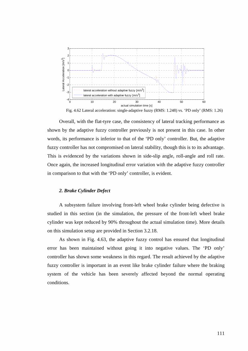
111
0 10 20 30 40 50 60-4
-3
-2
-1
0
1
2
3
actual simulation time [s]
Late
ral A
ccel
erat
ion
[m/s
2 ]
lateral acceleration without adaptive fuzzy [m/s2]
lateral acceleration with adaptive fuzzy [m/s2]
Fig. 4.62 Lateral acceleration: single-adaptive fuzzy (RMS: 1.248) vs. ‘PD only’ (RMS: 1.26)
Overall, with the flat-tyre case, the consistency of lateral tracking performance as
shown by the adaptive fuzzy controller previously is not present in this case. In other
words, its performance is inferior to that of the ‘PD only’ controller. But, the adaptive
fuzzy controller has not compromised on lateral stability, though this is to its advantage.
This is evidenced by the variations shown in side-slip angle, roll-angle and roll rate.
Once again, the increased longitudinal error variation with the adaptive fuzzy controller
in comparison to that with the ‘PD only’ controller, is evident.
2. Brake Cylinder Defect
A subsystem failure involving front-left wheel brake cylinder being defective is
studied in this section (in the simulation, the pressure of the front-left wheel brake
cylinder was kept reduced by 90% throughout the actual simulation time). More details
on this simulation setup are provided in Section 3.2.18.
As shown in Fig. 4.63, the adaptive fuzzy control has ensured that longitudinal
error has been maintained without going it into negative values. The ‘PD only’
controller has shown some weakness in this regard. The result achieved by the adaptive
fuzzy controller is important in an event like brake cylinder failure where the braking
system of the vehicle has been severely affected beyond the normal operating
conditions.

112
0 10 20 30 40 50 60-2
0
2
4
6
8
10
12
14
actual simulation time [s]
Long
itudi
nal E
rror
[m
]
longitudinal error without adaptive fuzzy [m]
longitudinal error with adaptive fuzzy [m]
Fig. 4.63 Longitudinal error: single-adaptive fuzzy (RMS: 3.159) vs. ‘PD only’ (RMS: 3.068)
Unlike, in the previous simulations, lateral error has shown some deterioration
with the adaptive fuzzy control in comparison to the ‘PD only’ control, as shown in Fig.
4.64, i.e. around the point 5 [s]. But, apart from that point, the adaptive fuzzy controller
has shown some positive trend in the rest of the time.
0 10 20 30 40 50 60-0.1
0
0.1
0.2
0.3
0.4
actual simulation time [m]
Late
ral E
rror
[m
]
lateral error with adaptive fuzzy [m]
lateral error without adaptive fuzzy [m]
Fig.4.64 Lateral error: single-adaptive fuzzy (RMS: 0.03453) vs. ‘PD only’ (RMS: 0.04876)
0 10 20 30 40 50 60-0.05
-0.04
-0.03
-0.02
-0.01
0
0.01
0.02
0.03
0.04
actual simulation time [s]
Pitc
h A
ngle
[ra
d]
pitch angle with adaptive fuzzy [rad]
pitch angle without adaptive fuzzy [rad]
Fig.4.65 Pitch angle: single-adaptive fuzzy (RMS: 0.01583) vs. ‘PD only’ (RMS: 0.01627)
The single adaptive fuzzy control has done well to keep the pitch angle low
throughout, in comparison to the ‘PD only’ control, as shown in Fig. 4.65. In the
meantime, as shown in Figs. 4.66, 4.67, the variations of roll angle and roll rate with the
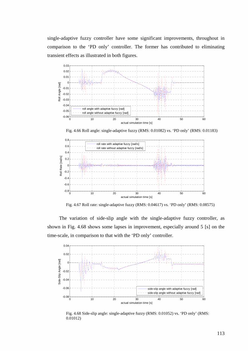
113
single-adaptive fuzzy controller have some significant improvements, throughout in
comparison to the ‘PD only’ controller. The former has contributed to eliminating
transient effects as illustrated in both figures.
0 10 20 30 40 50 60-0.06
-0.05
-0.04
-0.03
-0.02
-0.01
0
0.01
0.02
0.03
actual simulation time [s]
Rol
l Ang
le [
rad]
roll angle with adaptive fuzzy [rad]
roll angle without adaptive fuzzy [rad]
Fig. 4.66 Roll angle: single-adaptive fuzzy (RMS: 0.01082) vs. ‘PD only’ (RMS: 0.01183)
0 10 20 30 40 50 60-0.8
-0.6
-0.4
-0.2
0
0.2
0.4
0.6
0.8
actual simulation time [s]
Rol
l Rat
e [r
ad/s
]
roll rate with adaptive fuzzy [rad/s]
roll rate without adaptive fuzzy [rad/s]
Fig. 4.67 Roll rate: single-adaptive fuzzy (RMS: 0.04617) vs. ‘PD only’ (RMS: 0.08575)
The variation of side-slip angle with the single-adaptive fuzzy controller, as
shown in Fig. 4.68 shows some lapses in improvement, especially around 5 [s] on the
time-scale, in comparison to that with the ‘PD only’ controller.
0 10 20 30 40 50 60-0.08
-0.06
-0.04
-0.02
0
0.02
0.04
actual simulation time [s]
Sid
e-S
lip A
ngle
[ra
d]
side-slip angle with adaptive fuzzy [rad]
side-slip angle without adaptive fuzzy [rad]
Fig. 4.68 Side-slip angle: single-adaptive fuzzy (RMS: 0.01052) vs. ‘PD only’ (RMS: 0.01012)

114
Unlike in the previous cases, the variation of lateral acceleration as exhibited by
the adaptive fuzzy controller has been less satisfactory in comparison to that with the
‘PD only’ controller. This is shown in Fig. 4.69. The worst situation with the adaptive
fuzzy controller occurs around 42 [s], at which point the value peaks around 15 [m/s2].
Clearly, these values shown by the adaptive fuzzy controller exceed the normal design
specifications of the passenger vehicles as far as lateral acceleration is concerned [178].
0 10 20 30 40 50 60-20
-15
-10
-5
0
5
10
actual simulation time [s]
Late
ral A
ccel
erat
ion
[m/s
2 ]
lateral acceleration with adaptive fuzzy [m/s2]
lateral acceleration without adaptive fuzzy [m/s2]
Fig. 4.69 Lateral acceleration: single-adaptive fuzzy (RMS: 1.334) vs. ‘PD only’ (RMS: 1.351)
Overall, in the presence of a brake cylinder pressure failure, the performance of
the adaptive fuzzy controller provides some weaker responses with regard to lateral
tracking. This is an unfamiliar response as far as the previous results of the adaptive
fuzzy controller are concerned. On the other hand, there are some improvements with
regard to lateral stability as shown in the performances of side-slip angle, roll-angle and
roll rate. Quite strangely, the adaptive fuzzy control has shown some improved results
with regard to longitudinal error variation in comparison to that with the ‘PD only’
control.
Considering the overall performance of the single-adaptive fuzzy controller in
comparison to that with the ‘PD only’ controller, the following conclusions can be
drawn. There have been significantly positive results as far as lateral tracking is
concerned except in cases of failure modes. With regard to flat-tyre case, the results are
mixed. But, the performance is worse in the case of brake cylinder failure.
The lateral stability has been consistent with the adaptive fuzzy controller. But, as
far as longitudinal tracking is concerned, the performance of the adaptive fuzzy
controller is worse. There is a slight change in the brake cylinder failure case where the
adaptive fuzzy controller performance is slightly better.
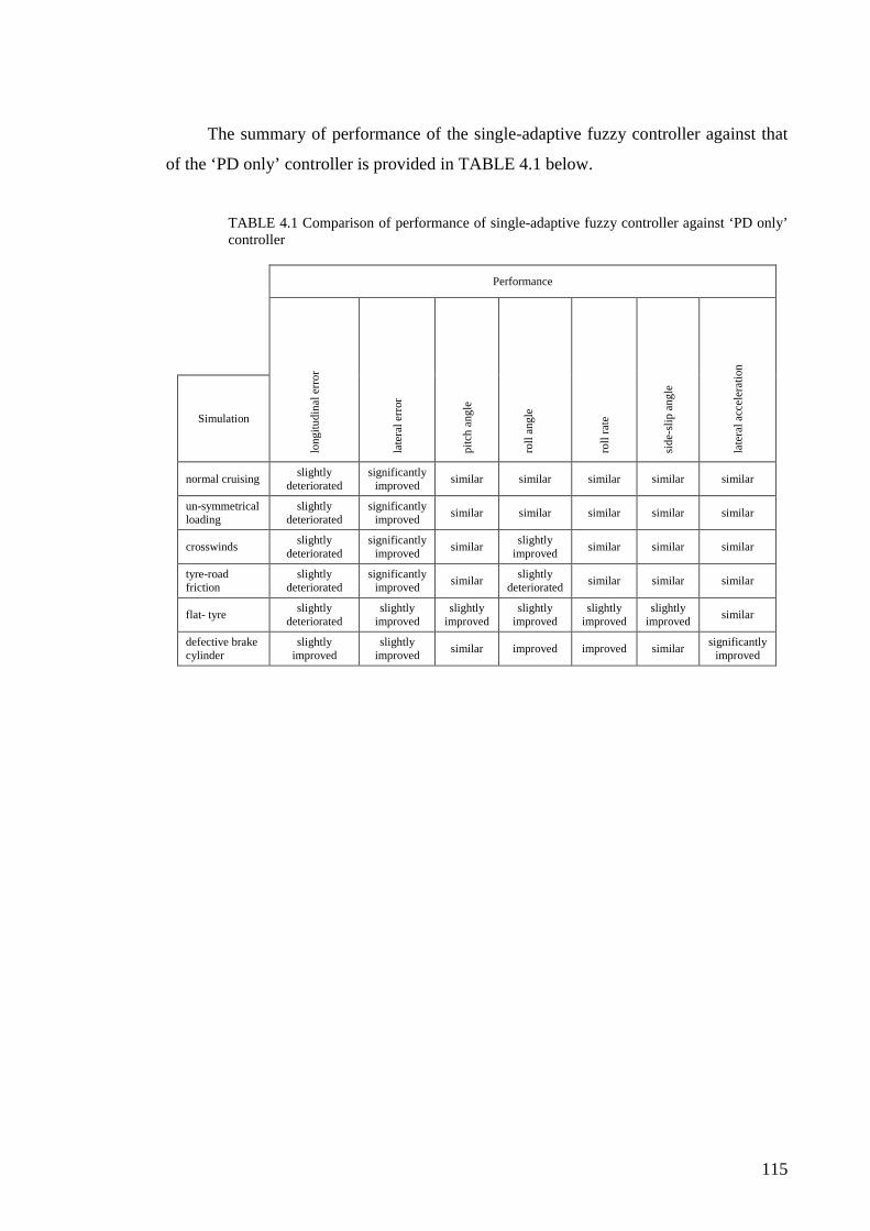
115
The summary of performance of the single-adaptive fuzzy controller against that
of the ‘PD only’ controller is provided in TABLE 4.1 below.
TABLE 4.1 Comparison of performance of single-adaptive fuzzy controller against ‘PD only’ controller
Performance
Simulation
long
itudi
nal e
rror
late
ral e
rror
pitc
h a
ngle
roll
ang
le
roll
rate
side
-slip
ang
le
late
ral a
cce
lera
tion
normal cruising slightly
deteriorated significantly
improved similar similar similar similar similar
un-symmetrical loading
slightly deteriorated
significantly improved
similar similar similar similar similar
crosswinds slightly
deteriorated significantly
improved similar
slightly improved
similar similar similar
tyre-road friction
slightly deteriorated
significantly improved
similar slightly
deteriorated similar similar similar
flat- tyre slightly
deteriorated slightly
improved slightly
improved slightly
improved slightly
improved slightly
improved similar
defective brake cylinder
slightly improved
slightly improved
similar improved improved similar significantly
improved
116
4.2 Chapter Summary
In this chapter, error dynamics for the single-adaptive fuzzy controller design is
described first. This is followed with a description of fuzzy system basics. Then a
detailed design of the single-adaptive fuzzy controller is described.
The procedure for determining the fuzzy controller parameters of the system a
priori using data, is described. This description includes how a number of vehicle runs
were conducted and data gathered. This is followed with a description on using the
subtractive clustering method and ANFIS method for determining the parameters for the
adaptive fuzzy controller using the gathered data.
A detailed robust stability analysis procedure is followed for ensuring asymptotic
stability of the single-adaptive fuzzy system using Lyapunov based KYP lemma. The
details of the developed controller being validated using a comprehensive set of
simulations on veDYNA®, are described. These details on the simulations include
testing of the controller for its robust qualities under a number of external disturbances
as well as a couple of failure modes.

117
C H A P T E R 5
Robust Multiple-Model Adaptive Fuzzy Control Systems – Blending (Soft-Switching) In this chapter, the design of two types of novel robust Multiple-Model/Multiple-
Controllers (MM/MC) based on fuzzy systems is described. They are designed to
address the integrated lateral and longitudinal control of highway vehicles. The first
controller type discussed in this chapter is ‘robust multiple-adaptive fuzzy controller’,
which is comprised of a number of adaptive fuzzy controllers tuned differently for
addressing different dynamic situations. These adaptive fuzzy controllers are ‘blended’
using a ‘fixed-parameter’ fuzzy function to obtain a single control output. The second
controller, ‘robust fuzzy PDC (Parallel Distributed Compensation) based MM/MC
fuzzy controller’ is comprised of many local adaptive fuzzy controllers that are blended
using a fuzzy PDC structure. The design of the fuzzy PDC system is based on the
sector-nonlinearity method. Both controllers are established with stability based on a
Lyapunov-based method, i.e. KYP lemma, leading to asymptotic stability at large. The
two controller systems developed are validated with comprehensive set of simulation
studies on veDYNA® and MATLAB/Simulink®, in the presence of many external
disturbances and non-catastrophic subsystem failures.
118
5.1 Robust Multiple-Adaptive Fuzzy Control Systems with ‘Blending’ (Soft-Switching)
5.1.1 Introduction
It has already been highlighted in the main introduction that there are drawbacks
in using single-model (or single ‘modal’) control systems in addressing the problem of
integrated lateral and longitudinal control of highway vehicles.
Since MM/MC systems have more built-in capability to address control
requirements with improved tracking with higher reliability, it is more relevant and
applicable to use them within an Automated Highway System (AHS).
Therefore, in this section, the development of a robust multiple-adaptive fuzzy
control system based on blending is described in order to address the problem of
integrated lateral and longitudinal control of highway vehicles. By fuzzy blending of a
number of inputs from a bank of suitably configured adaptive fuzzy controllers, the
uncertainty between the vehicle and the vehicle-model is modelled. The design of the
multiple-adaptive fuzzy controller is based on having ‘controller-signals as inputs’ in
the fuzzy (blender) system. Having many adaptive fuzzy systems as multiple-controllers
enables one to effectively define and model uncertainty of the system over which the
control action is developed.
5.1.2 Synthesis of Multiple-Adaptive Fuzzy Controller with Blending
This section presents a comprehensive synthesis of a novel setup of a robust
multiple-adaptive fuzzy control system. In this multiple-controller setup, a number of
adaptive fuzzy controllers are configured specifically considering a variety of scenarios.
These individual adaptive fuzzy controllers operate in parallel and their output control
signals are blended using another ‘fixed-parameter’ fuzzy system. Blending of adaptive
fuzzy controller in the fixed fuzzy system is according to pre-identified or tuned output
membership parameters. This pre-identification of fixed parameters is done using a
generic scenario of operation, e.g. normal cruising conditions where there are no
119
external disturbances. Since the system is quite versatile with the addition of multiple-
adaptive fuzzy controllers, it can be used to cover different ‘scenarios’ or ‘modes’ in
multiple-environments of vehicle operation.
The input variables of ‘fuzzy blender’ (a T–S fuzzy system) of the control system
consist of outputs of individual adaptive fuzzy controllers. Though this inclusion makes
the analysis of stability of the system complicated, it helps to track the input space more
effectively. In this system each adaptive fuzzy controller is tuned using an online
feedback signal from the blending fuzzy function. Therefore, the whole system creates a
unique adaptable system of controllers where versatility is high in comparison to single-
model control systems. Hence, the developed system produces a more reliable and
accurate control system in comparison to a single-model controller.
Since the adaptive fuzzy controller outputs are blended using ‘IF –THEN’ rules of
the fuzzy blender, such an input space can be considered as providing a measure of
‘identification’ of a state-space characteristic that is based on individual states or
combination of states of the system. Therefore this arrangement improves identification
of a particular scenario. This improvement can be compared against a few states of the
system identifying a ‘characteristic’ or ‘condition’ of the control space before applying
a control signal in the normal manner. But, the method adopted in this multiple-adaptive
controller provides a more versatile ‘identification’. This process is part of mapping by
individual adaptive fuzzy controllers that have more capability to identify a wider
spectrum of ‘behaviour’ of the system.
(i) Design of Multiple-Adaptive Fuzzy Controllers with Fuzzy Blender
The following Fig. 5.1 shows the schematic diagram of the robust multiple-
adaptive fuzzy controller with fuzzy blender. In this control system setup, the outputs of
the bank of adaptive fuzzy controllers, Tj jψ θ where j = 1, …, n (where ( 1)n > ∈N is
the number total number of adaptive fuzzy controllers in the bank), are blended using a
fuzzy blender. The resulting output from the fuzzy blender is used to complement the
PD (proportional-derivative) output, and is used to model the ‘uncertainty’ between the
vehicle and vehicle-model.
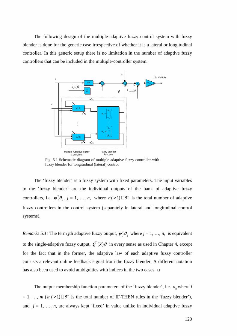
120
The following design of the multiple-adaptive fuzzy control system with fuzzy
blender is done for the generic case irrespective of whether it is a lateral or longitudinal
controller. In this generic setup there is no limitation in the number of adaptive fuzzy
controllers that can be included in the multiple-controller system.
Fig. 5.1 Schematic diagram of multiple-adaptive fuzzy controller with fuzzy blender for longitudinal (lateral) control
The ‘fuzzy blender’ is a fuzzy system with fixed parameters. The input variables
to the ‘fuzzy blender’ are the individual outputs of the bank of adaptive fuzzy
controllers, i.e. Tj jψ θ , j = 1, …, n, where ( 1)n > ∈N is the total number of adaptive
fuzzy controllers in the control system (separately in lateral and longitudinal control
systems).
Remarks 5.1: The term jth adaptive fuzzy output, Tj jψ θ where j = 1, …, n, is equivalent
to the single-adaptive fuzzy output, ( )T x θξ in every sense as used in Chapter 4, except
for the fact that in the former, the adaptive law of each adaptive fuzzy controller
consists a relevant online feedback signal from the fuzzy blender. A different notation
has also been used to avoid ambiguities with indices in the two cases.
The output membership function parameters of the ‘fuzzy blender’, i.e. ija where i
= 1, …, m ( ( 1)m > ∈N is the total number of IF-THEN rules in the ‘fuzzy blender’),
and j = 1, …, n, are always kept ‘fixed’ in value unlike in individual adaptive fuzzy
su PD
⋮
e
e
-
eɺ
Multiple Adaptive Fuzzy Controllers
1Tα ς
Tnα ς
( )p sx l ɺɶɺ ψ ν
ˆ ( )h xɺ
( , )ˆ ( )s x yh q
Fuzzy Blender
Function
11
1
1m
a
a
α =
⋮
⋮ 1n
n
nm
a
a
α =
⋮
,1 x yb
1 1Tψ θ
Tn nψ θ
s
t∆∆
+ + +
e
To Vehicle
121
controllers (in adaptive fuzzy controllers, only the output membership function
parameters are ‘adaptive’).
Let the IF-THEN rules of ‘fuzzy blender’ (a T–S fuzzy system) be,
1R :
IF 1 1Tψ θ is 1
qF AND … AND T
n nψ θ is 1rF THEN
1 11 1 1 1( ) ... ( )T Tn n nz a a= + +ψ θ ψ θ
⋮
mR :
IF 1 1Tψ θ is q
mF AND … AND Tn nψ θ is r
mF THEN (5.1)
1 1 1( ) ... ( )T Tm m mn n nz a a= + +ψ θ ψ θ
where Tj jψ θ is the control output from the jth adaptive fuzzy controller (jψ is the
regression vector and jθ is the parameter set of the jth controller) where 1, ,j n= … . iz
is the ith ( 1, ,i m= … ( ( 1)m > ∈N )) consequent membership function where m is the
total number of IF–THEN rules in the ‘fuzzy blender’.
The tuning of each adaptive fuzzy controller, T
j jψ θ where 1, ,j n= … is done with
an adaptive law (derived in the stability analysis process) consisting of two parts:
‘internal’ and ‘external’. The internal part of the adaptive law consists of the system
error, and the external part consists of a relevant online ‘feedback signal’ from the
‘fuzzy blender’, i.e. Tjα ς to the jth adaptive fuzzy controller where 1, ,j n= … (the term
Tjα ς is explained in the Lyapunov stability analysis). The input variables to each
adaptive fuzzy controller are ‘error’ and ‘error rate'.
Having each adaptive law as a function of a relevant online feedback signal from
the fuzzy blender is advantageous. This allows one to change each set of adaptive
parameters in each adaptive fuzzy controller with respect to the fixed set of parameters
of the fuzzy blender. Therefore, adaptation in each adaptive fuzzy controller becomes a
‘global’ phenomenon as against a purely ‘local’ one.
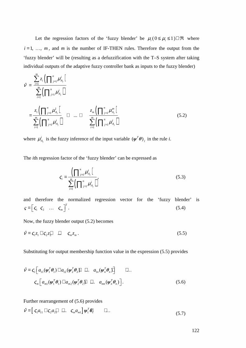
122
Let the regression factors of the ‘fuzzy blender’ be iµ ( 0 1iµ≤ ≤ )∈R where
1, ,i m= … , and m is the number of IF-THEN rules. Therefore the output from the
‘fuzzy blender’ will be (resulting as a defuzzification with the T–S system after taking
individual outputs of the adaptive fuzzy controller bank as inputs to the fuzzy blender)
( )( )
11
11
ˆj
j
mn i
i Aji
mn i
Aji
z µν
µ
==
==
=∑ ∏
∑ ∏
( )( )
( )( )
11 1 1
1 11 1
...j j
j j
n n mA m Aj j
m mn ni i
A Aj ji i
z zµ µ
µ µ
= =
= == =
= + +∏ ∏
∑ ∑∏ ∏ (5.2)
where
j
iAµ is the fuzzy inference of the input variable ( )T
jψ θ in the rule i.
The ith regression factor of the ‘fuzzy blender’ can be expressed as
( )( )
1
11
j
j
n iAj
i mn i
Aji
µς
µ
=
==
=∏
∑ ∏, (5.3)
and therefore the normalized regression vector for the ‘fuzzy blender’ is
1 2
T
mς ς ς = ς … . (5.4)
Now, the fuzzy blender output (5.2) becomes
1 1 2 2ˆ ... m mz z zν ς ς ς= + + + . (5.5)
Substituting for output membership function value in the expression (5.5) provides
1 11 1 1 12 2 2 1ˆ ( ) ( ) .... ( )T T Tn n na a aν ς = + + + + + ψ θ ψ θ ψ θ …
1 1 1 2 2 2( ) ( ) .... ( )T T Tm m m mn n na a aς + + + ψ θ ψ θ ψ θ . (5.6)
Further rearrangement of (5.6) provides
[ ]1 11 2 21 1 1 1ˆ .... Tm ma a aν ς ς ς= + + + + +ψ θ …
(5.7)

123
[ ]1 1 2 2 .... Tn n m mn n na a aς ς ς+ + + ψ θ .
Separating the expression (5.7) into individual vectors provides
[ ] [ ]11 1
21 21 2 1 1 1 2
1
ˆ . . .
n
nT Tm m n n
m mn
a a
a a
a a
ν ς ς ς ς ς ς
= + +
ψ θ ψ θ⋯ ⋯⋮ ⋮
. (5.8)
Once again, contracting the expression (5.8) with vector symbols provides
1 1 1 2 2 2ˆ ( ) ( ) ( )T T T Tn n nν = + + + ς α ψ θ α ψ θ α ψ θ… . (5.9)
Finally, it results in as
ν ( )1( )
nT Tj j jj =
= ∑ς α ψ θ . (5.10)
Remark 5.2: Though (5.10) is generally nonlinear, it is linear with respect to its
unknown parameters. Hence, parameter adaptation algorithms applicable for linear
systems, e.g. gradient-based algorithms, can be readily used in estimation of the
unknown parameters in (5.10) [27].
For the jth adaptive fuzzy controller, the regression vector can be expressed as
1 2, ,T
j j j jp = ψ ψ ψ ψ⋯ . Thereby the kth element of jth controller becomes
Tjk jk jk jke eψ ψ ψ = = ψ eɺ where 1, ,j n= ⋯ (n is the total number of
controllers), and 1, ,k p= ⋯ where ( 1)p > ∈N is the total number of IF-THEN fuzzy
rules in each adaptive fuzzy controller.
Each output membership function parameter set of each adaptive fuzzy controller
can be tuned using an algorithm based on an adaptive law. For the jth adaptive fuzzy
controller, this adaptive law becomes
j j j jγ= − Tθ ψ α ςCeɺɶ (5.11)
where 1, ,j n= ⋯ (n is the number of adaptive fuzzy controllers).

124
(ii) Control Law
The certainty equivalence control laws for the longitudinal and lateral control of
the vehicle are, respectively
( )1
1 ˆˆ ( ) ( )nT T
x p dx x px x j j j sx x sjxx
u x k e k e u h qb = = + + + + −
∑ς α ψ θɺɺ ɺ ɺ (5.12)
( )1
1 ˆˆ ( ) ( ) .s
nT Ty s dy y py y j j j sy y sj
yy
u l k e k e u h qb =
= + + + + − ∑ς α ψ θɺɺɶ ɺ ɺψ (5.13)
Here, 1 2
T
mς ς ς = ς … is the regression matrix of the fuzzy blender where
iς ( 0 1iς≤ ≤ )∈R , 1, ,i m= … is the ith fuzzy regression factor. This fuzzy blender
does the blending of each adaptive fuzzy controller output (for jth controller it is Tj jψ θ
where 1, ,j n= ⋯ ) together, and thereby generates a unique output. Each 1 2, , , nθ θ θ⋯
provides parameter matrices for each adaptive fuzzy controller.
Here, ,ˆ ( )
sx y sh qɺ denotes the calculated value of the term , ( )sx y sh qɺ .
( )1ˆ ( )
nT Tx j j jj
xν
== ∑ς α ψ θ and ( )1
ˆ ( )nT T
y j j jjy
ν=
= ∑ς α ψ θ are the outputs from the
multiple-adaptive fuzzy controller for longitudinal and lateral cases, respectively. dxk ,
pxk are the constant PD (proportional-derivative) gains for the longitudinal controller,
and dyk , pyk are the constant PD gains for the lateral controller. s sx syu u u = is the
variable structure control term.
(iii) Error Dynamics
Equation (5.12) can be substituted in the vehicle model equation (3.4), and
thereby it can be rearranged to have the longitudinal error dynamics as
( )1
*
ˆ ( ) ( ) ( )
ˆ
.
nT Tx dx x px x x s x s j j j sx xj
x
x x x sx x
x sx x
e k e k e h q h q u d
w u d
u d
ν ν
ν
=+ + = − − − −
= + − − −
= − −
∑ς α ψ θɺɺ ɺ ɺ ɺ
ɶ
(5.14)
In the same manner, using (5.13) and (3.5), lateral error dynamics will result in as

125
( )1
*
ˆ ( ) ( ) ( )
ˆ
.
s s
nT Ty dy y py y y s y s j j j sy yj
y
y y y sy y
y sy y
e k e k e h q h q u d
w u d
u d
ν ν
ν
=+ + = − − − −
= + − − −
= − −
∑ς α ψ θɺɺ ɺ ɺ ɺ
ɶ
(5.15)
In this discussion, * * *
x yν ν ν = is the optimal adaptive fuzzy output while
ˆ ˆ ˆx yν ν ν = is the actual adaptive fuzzy output. xw , yw are the adaptive fuzzy
approximation errors. These errors are bounded by x xw W< and y yw W< where
xW , yW ∈R are the practical bounds.
By using the universal approximation theorem (provided in Chapter 4), with the
fuzzy adaptation process, the fuzzy controller parameters can be gradually brought to
the optimal values. Thus the right half of the equations (5.14) and (5.15) can be made
zero.
The variable structure term,su is used to balance the effects of fuzzy
approximation errors. The overall uncertainty factor in the equation is made zero with
the fuzzy function.
The detailed design of each adaptive fuzzy controller (e.g. jth adaptive fuzzy
controller, Tj jψ θ , where 1, ...,j n= ) is provided in Chapter 4 under the topic of single-
model adaptive fuzzy systems.
5.1.3 Training of Multiple-Adaptive Fuzzy Controller Parameters
(i) Training of Adaptive Fuzzy Controllers
The set of adaptive fuzzy controllers in the control system can be used in a
number of different ways.
Firstly, the controllers can be trained with a data set (obtained from running a
vehicle through a real scenario), similar to that with the ‘single model adaptive fuzzy
controller’ discussed in Chapter 4. This data is for tuning the input and output

126
membership parameters of the adaptive fuzzy controllers. Then the adaptive rates in the
adaptive law can be changed to differentiate each controller from the other. The
adaptive fuzzy controllers having ‘higher adaptive rate’ can be used in the faster
changing scenarios whereas the controllers having ‘lower adaptive rate’ can be used
with low frequency changes in the scenarios. Since each controller is trained on the
same set of ‘global’ data, each controller can act globally.
Instead of having a common data set for training each of adaptive fuzzy
controllers, data space can be categorized into groups, e.g. according to the frequency of
change of the variable ‘error’, i.e. error rate. Thereby, using each of the ‘local’ data
sets, a single adaptive fuzzy controller can be trained. It is clear that blending each of
the controllers will address the ‘global’ scenarios having full ‘spectrum’ of frequencies
of operation. This is another option for tuning the adaptive fuzzy controllers. But, the
first option will be followed in the design of the control system.
Using the subtractive clustering method, the fuzzy membership function centres
and standard deviations (Gaussian) have been obtained. Then the basic fuzzy structure
obtained using the subtractive clustering method is further tuned using ANFIS with the
gathered data from veDYNA®. The details of the tuning process are explained below.
(ii) Training of Fuzzy Blender Function
The fixed parameter fuzzy blender of the multiple-adaptive fuzzy system was
tuned as follows. The tuning of the fuzzy blender was done considering only two
adaptive fuzzy controllers as inputs in each longitudinal and lateral case. The adaptive
rates of the adaptive fuzzy controllers were chosen as 0.03 and 0.04 in the longitudinal
controller, and 0.01 and 0.03 in the lateral controller.
The following tuning procedure of the fuzzy blender was adopted in general,
irrespective of the lateral or longitudinal controller.
In each kth trial, the output for the fuzzy blender was calculated using the equation
ˆˆ ( ) ( )i i s i sk kkh q h qν = −ɺ ɺ (5.16)
where ,i x y= for longitudinal and lateral cases respectively. The vehicle dynamics,
( )i sh qɺ was calculated using BMW 325i 1988 model of veDYNA®, and the vehicle

127
model dynamics, ( )i sh qɺ was calculated using equation (3.7).
The tuning procedure of the fuzzy blender is described as follows:
i) First, by setting the output membership function parameters of the blender as ‘ones’
(i.e. ‘1’s), data was collected for the output of the blender, following a profile of vehicle
simulation trial on veDYNA®. This data collection was similar to the case of the single
adaptive fuzzy system, as described in Section 4.3.
ii) Using the output data obtained in (i), and together with the two adaptive fuzzy
controller outputs taken as the two inputs to the fuzzy blender, a basic fuzzy structure
was generated using the subtractive clustering method. The same set of data has been
used further to obtain a more refined fuzzy structure for the fuzzy blender using the
ANFIS method. The fuzzy blender structure from the first trial was thus obtained.
iii) Once the first set of parameters (parameters from the first trial) of the fuzzy blender
was identified, taking these parameters as the current working setup for the next trial, a
new data set was collected. The same profile of vehicle simulation trial on veDYNA®
was followed. The data obtained was used to work out the new fuzzy blender structure
in the same way as discussed in (i) and (ii). This structure was taken as the fuzzy
blender for the second trial.
The trials of optimizing the fuzzy blender parameters were continued until there
was no change of value that was more than 5% of the output of the fuzzy blender.
Thereby, using the final set of data, the parameters of the fuzzy blender were identified.
(a) Training Data: Longitudinal
Figs. 5.2 and 5.3 show the inputs and the output for tuning the longitudinal fuzzy
blender in the first trial. More details on validation of developed fuzzy models are
provided in Section 4.1.5.

128
Inputs
0 200 400 600 800 1000 1200 1400 1600 1800 2000-80
-70
-60
-50
-40
-30
-20
-10
0
10
data number
Fuz
zy B
lend
er I
nput
Controller 1
Controller 2
Fig. 5.2 Train data (inputs) for ANFIS training of longitudinal fuzzy blender
Output
0 200 400 600 800 1000 1200 1400 1600 1800 2000-0.2
-0.1
0
0.1
0.2
0.3
0.4
0.5
Data Number
Fuz
zy B
lend
er O
utpu
t
Fig. 5.3 Train data (output) for ANFIS training of longitudinal fuzzy blender
The ANFIS training and checking errors for tuning the longitudinal fuzzy blender
in the first trial are shown in Figs. 5.4 and 5.5, respectively.
0 10 20 30 40 50 60 70 80 90 1000
0.02
0.04
0.06
0.08
0.1
0.12
Iteration Number
Long
itudi
nal T
rain
Err
or
Fig. 5.4 Training error for ANFIS training of longitudinal fuzzy blender
The fuzzy blender parameters that were associated with the lowest error in the
checking (validation) were selected as the final values. This validation error is as shown
in Fig. 5.5.
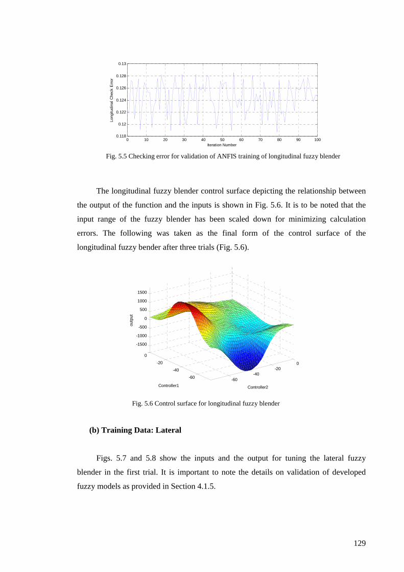
129
0 10 20 30 40 50 60 70 80 90 1000.118
0.12
0.122
0.124
0.126
0.128
0.13
Iteration Number
Long
itudi
nal C
heck
Err
or
Fig. 5.5 Checking error for validation of ANFIS training of longitudinal fuzzy blender
The longitudinal fuzzy blender control surface depicting the relationship between
the output of the function and the inputs is shown in Fig. 5.6. It is to be noted that the
input range of the fuzzy blender has been scaled down for minimizing calculation
errors. The following was taken as the final form of the control surface of the
longitudinal fuzzy bender after three trials (Fig. 5.6).
-60-40
-200
-60
-40
-20
0
-1500
-1000
-500
0
500
1000
1500
Controller2Controller1
outp
ut
Fig. 5.6 Control surface for longitudinal fuzzy blender
(b) Training Data: Lateral
Figs. 5.7 and 5.8 show the inputs and the output for tuning the lateral fuzzy
blender in the first trial. It is important to note the details on validation of developed
fuzzy models as provided in Section 4.1.5.
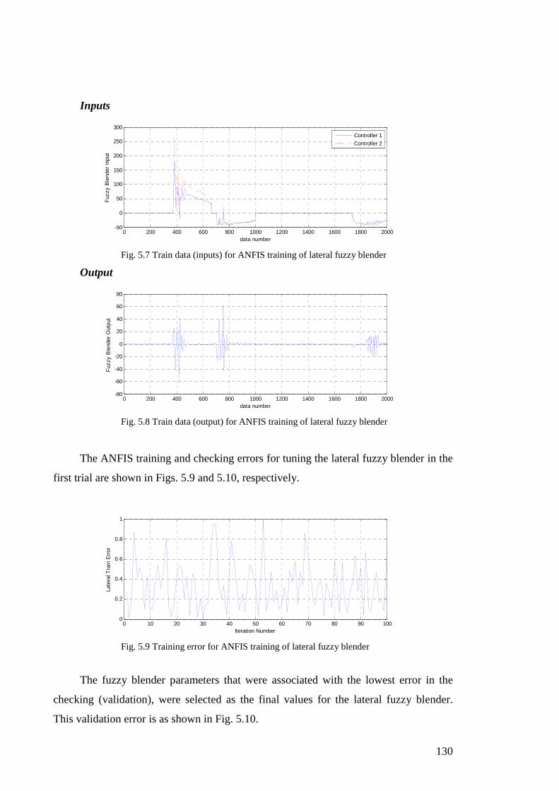
130
Inputs
0 200 400 600 800 1000 1200 1400 1600 1800 2000-50
0
50
100
150
200
250
300
data number
Fuz
zy B
lend
er I
nput
Controller 1
Controller 2
Fig. 5.7 Train data (inputs) for ANFIS training of lateral fuzzy blender
Output
0 200 400 600 800 1000 1200 1400 1600 1800 2000-80
-60
-40
-20
0
20
40
60
80
data number
Fuz
zy B
lend
er O
utpu
t
Fig. 5.8 Train data (output) for ANFIS training of lateral fuzzy blender
The ANFIS training and checking errors for tuning the lateral fuzzy blender in the
first trial are shown in Figs. 5.9 and 5.10, respectively.
0 10 20 30 40 50 60 70 80 90 1000
0.2
0.4
0.6
0.8
1
Iteration Number
Late
ral T
rain
Err
or
Fig. 5.9 Training error for ANFIS training of lateral fuzzy blender
The fuzzy blender parameters that were associated with the lowest error in the
checking (validation), were selected as the final values for the lateral fuzzy blender.
This validation error is as shown in Fig. 5.10.

131
0 10 20 30 40 50 60 70 80 90 1000
0.5
1
1.5
Iteration Number
Late
ral C
heck
Err
or
Fig. 5.10 Checking error for validation of ANFIS training of lateral fuzzy blender
The lateral fuzzy blender control surface depicting the relationship between the
output of the function and the inputs is shown in Fig. 5.11. It is to be noted that the
input range of the fuzzy blender has been scaled down for minimizing calculation
errors. Fig. 5.11 shows the final form of the control surface of the lateral fuzzy bender
after three trials.
-300-200
-1000
100
-400-300
-200-100
0100
-60
-40
-20
0
Controller2Controller1
outp
ut
Fig. 5.11 Control surface for lateral fuzzy blender
The final tuned input and output membership function parameters of the fuzzy
blender in longitudinal and lateral forms are provided in APPENDIX C.

132
5.1.4 Robust Stability Analysis of Control System
The following stability proof of the developed multiple-adaptive fuzzy control
system with fuzzy blender is carried out for the generic case irrespective whether it is
lateral or longitudinal controller. Therefore, the subscripts that are specific to either the
longitudinal or lateral case are removed in this description. Nevertheless, the specific
details will be mentioned as and when necessary.
Assumption 5.1: The sum of fuzzy approximation errors, w is bounded, i.e., w W≤
where ( 0)W > ∈R . The external disturbances, d are bounded too, i.e., d D≤ where
( 0)D > ∈R . Thereby the variable structure control gain is chosen as f W Dσ ≥ + .
The main features of the robust multiple adaptive fuzzy control system with
‘blending’ can be summarized in the following theorem.
Theorem 5.1: Let the parameter vectors, jθ of the adaptive fuzzy systems be adjusted
by the adaptive law as provided in (5.11) and let Assumption 5.1 be true. The proposed
adaptive fuzzy control law as provided in (5.12) [and (5.13)] can guarantee stability of
the vehicle system with the following properties:
i) The closed loop vehicle system is stable, i.e. ∈e ∞L , considering lateral and
longitudinal cases separately.
ii) The system errors and the parametric errors are asymptotically stable, i.e.
lim 0t x ye , e→∞ = , and lim 0t jθ→∞ =ɶ for 1, ...,j n= where n is the total number of
adaptive fuzzy controllers in the control system (considering lateral and
longitudinal cases separately).
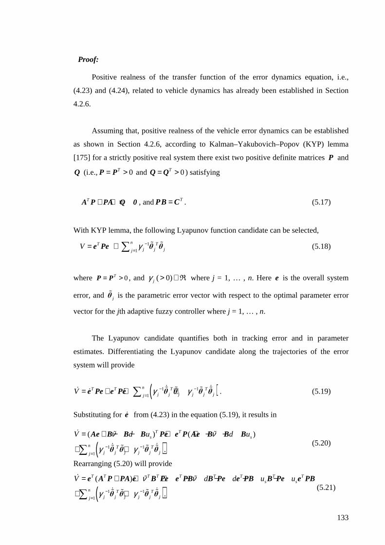
133
Proof:
Positive realness of the transfer function of the error dynamics equation, i.e.,
(4.23) and (4.24), related to vehicle dynamics has already been established in Section
4.2.6.
Assuming that, positive realness of the vehicle error dynamics can be established
as shown in Section 4.2.6, according to Kalman–Yakubovich–Popov (KYP) lemma
[175] for a strictly positive real system there exist two positive definite matrices P and
Q (i.e., 0T= >P P and 0T= >Q Q ) satisfying
T + + =A P PA Q 0, and T=PB C . (5.17)
With KYP lemma, the following Lyapunov function candidate can be selected,
1
1
nT Tj j jj
V γ −=
= + ∑e Pe θ θɶ ɶ (5.18)
where 0T= >P P , and ( 0)jγ > ∈R where j = 1, … , n. Here e is the overall system
error, and jθɶ is the parametric error vector with respect to the optimal parameter error
vector for the jth adaptive fuzzy controller where j = 1, … , n.
The Lyapunov candidate quantifies both in tracking error and in parameter
estimates. Differentiating the Lyapunov candidate along the trajectories of the error
system will provide
( )1 1
1
nT T T Tj j j j j jj
V γ γ− −=
= + + +∑e Pe e Pe θ θ θ θɺ ɺɶ ɶ ɶ ɶɺ ɺ ɺ . (5.19)
Substituting for eɺ from (4.23) in the equation (5.19), it results in
( )1 1
1
( ) ( )
.
T Ts s
n T Tj j j j j jj
V d u d uν ν
γ γ− −=
= + − − + + − −
+ +∑
Ae B B B Pe e P Ae B B B
θ θ θ θ
ɺ ɶ ɶ
ɺ ɺɶ ɶ ɶ ɶ (5.20)
Rearranging (5.20) will provide
( )1 1
1
( )
.
T T T T T T T T Ts s
n T Tj j j j j jj
V d d u uν ν
γ γ− −=
= + + + − − − −
+ +∑
e A P PA e B Pe e PB B Pe e PB B Pe e PB
θ θ θ θ
ɺ ɶ ɶ
ɺ ɺɶ ɶ ɶ ɶ(5.21)

134
With the Lyapunov equation 0T + + =A P PA Q where 0T= >Q Q , (5.21) can be
further simplified as
( )( ) ( )1 1
1.
nT T T T T T T Ts j j j j j jj
V d uν ν γ γ− −=
= − + + − + + + +∑e Qe B Pe e PB B Pe e PB θ θ θ θɺ ɺɶ ɶ ɶ ɶɺ ɶ ɶ
(5.22)
From the argument, it can be expressed as * ˆ( )ν ν ν τ= − +ɶ where ν is the input
from the fuzzy blending function. *ν is the optimum fuzzy input, and τ is the
approximation error of the fuzzy blending function. It can be further elaborated that
( ) ( )*
1 1 1ˆ( ) ( )
n n nT T T Tj j j j j j jj j j
wν= = =
= − +∑ ∑ ∑ς α ψ θ ς α ψ θɶ (5.23)
where * 2p
j×∈θ R is the optimal parameter matrix for the jth adaptive fuzzy controller.
ˆjθ is the parameter set of the jth adaptive fuzzy controller, and jw is approximation
error of the jth adaptive fuzzy controller. This error is bounded, jw W≤ , i.e.
jw ∞∈L where W ∈R is a positive constant.
Equation (5.23) can be further simplified so that
( )*
1 1ˆ( )
n nT Tj j j j jj j
wν= =
= − +∑ ∑ς α ψ θ θɶ . (5.24)
Let 1
n
jjw w
==∑ where ( )w W< ∈R is a positive constant, and let the parameter error
be taken as * ˆj j j= −θ θ θɶ . The determination of fuzzy approximation error upper bound,
W has been discussed before [30].
Therefore equation (5.24) now becomes
( )1
nT Tj j ji
wν=
= +∑ς α ψ θɶɶ . (5.25)
Substituting (5.25) in (5.22) provides
( ) ( )( )( ) ( )
1 1
1 1
1.
Tn nT T T T T T T
j j j j j jj j
nT T T Ts j j j j j jj
V w w
d u γ γ
= =
− −=
= − + + + +
− + + + +
∑ ∑
∑
ɶ ɶɺ
ɺ ɺɶ ɶ ɶ ɶ
e Qe ς α ψ θ B Pe e PB ς α ψ θ
B Pe e PB θ θ θ θ
(5.26)
Since T=PB C , it can be further simplified to provide

135
( ) ( )( ) ( )( )
1 1
1 1
1
( ) ( )
.
n nT T T T T Tj j j j j jj j
n T T T Tj j j j j j sj
V
w d uγ γ
= =
− −=
= − + +
+ + + − − +
∑ ∑
∑
ɶ ɶɺ
ɺ ɺɶ ɶ ɶ ɶ
Te Qe θ ψ α ςCe e C ς α ψ θ
θ θ θ θ Ce e C (5.27)
Further rearrangement of (5.27) will result in
( )( )( )( )( )( ) ( )( )
1
1
1
1.
nT T T T Tj j j j jj
n T T T Tj j j j j sj
V
w d u
γ
γ
−=
−=
= − + +
+ + + − − +
∑
∑
Te Qe e Cς α ψ θ θ
θ ψ α ςCe θ Ce e C
ɺɶ ɶɺ
ɺɶ ɶ (5.28)
Now, (5.28) can be rearranged and written as
( )( )( ) ( )( )
1
1
1
1.
TnT T
j j j j jj
n T T T Tj j j j j sj
V
w d u
γ
γ
−=
−=
= − + +
+ + + − − +
∑
∑
e Qe ψ α ςCe θ θ
θ ψ α ςCe θ Ce e C
ɺɶ ɶɺ
ɺɶ ɶ
(5.29)
If the adaptive law as provided in (5.11), i.e., j j j jγ= − Tθ ψ α ςCeɺɶ , is substituted in the
equation (5.29), it can be reduced to
( )( )T T TsV w d u= − + − − +e Qe Ce e Cɺ . (5.30)
Equation (5.30) can be further expressed as
( )( )2
minT T
sV w d uλ≤ − + − − +Q e Ce e Cɺ (5.31)
where minλQ is the minimum eigen value of Q . Since fuzzy systems follow universal
approximation theorem [29], w may be made arbitrarily small by making each jw
small by proper choice of each fuzzy system if each ˆTj jψ θ is smooth (note that this may
require an arbitrarily large number of rules for each controller) [30].
Since disturbances are bounded, i.e., d D< , and it is known that w W< , it can be
further expressed that
( )( )2
minT T
sV D W uλ≤ − + + − +Q e Ce e Cɺ . (5.32)

136
Let the variable structure control term be ( )T Ts fu signσ= +Ce e C . Thereby, (5.32) can
be expressed as
( )2
minT T
fV D Wλ σ≤ − + + − +Q e Ce e Cɺ . (5.33)
Further arrangement of (5.33) will provide
( )2
minT T
fV D Wλ σ≤ − − + − +Q e Ce e Cɺ . (5.34)
If it is taken as f D Wσ ≥ + , then (5.34) will establish that
0V ≤ɺ , t∀ . (5.35)
Therefore, according to the Lyapunov theory, it establishes the fact that e is
bounded, i.e. ∞∈e L . Therefore, ,e eɺ are bounded, i.e. ,e e ∞∈ɺ L . It also establishes that
parameter errors are bounded, i.e. ∞∈θɶ L .
Equation (5.34) also implies that
2
minV λ≤ − Q eɺ . (5.36)
Integrating (5.36) will provide
2
min 0 0(0) ( )dt Vdt V Vλ
∞ ∞≤ − = − ∞∫ ∫Q e ɺ . (5.37)
Therefore, rearranging (5.37) will provide
( )min
2 1
0(0) ( )dt V Vλ
∞≤ − ∞∫ Q
e . (5.38)
Equation (5.38) leads to
2∈e L 2 2
0( ) : ( )z t z t dt
∞ = < ∞ ∫L (5.39)
since it provides (0), ( )V V ∞∞ ∈L according to (5.35) [30]. Since it can be proved as
2e ∞∈L L∩ (from (5.39) and (5.35)), and e ∞∈ɺ L (from (5.36)), by Barbalat’s lemma
[30], [176], it leads to asymptotic stability of e (i.e. lim 0t e→∞ = ). This can be extended
specifically to lateral and longitudinal cases, and consequently the lateral and
longitudinal errors are asymptotically stable, i.e.

137
lim 0.t x ye , e→∞ = (5.40)
This asymptotic stability result, as provided by (5.40) proves that when lateral and
longitudinal cases are considered at the same time, with the given arguments, the system
of errors can be proved asymptotically stable. Therefore, this result logically proves that
the integrated lateral and longitudinal control system is asymptotically stable. This
statement completes the proof of stability for the robust multiple-adaptive fuzzy
controller system based on blending.
The following definition is provided to formerly identify the variable vector
spaces, and thereby to define the optimal parameter set.
Definition 5.1: It is possible to define the compact parameter spaces for θ and x
variables. Let ( 0)Mθ > ∈R and ( 0)xM > ∈R be finite, and
:j j Mθ = ∈ ≤θ
Ω θ θR , and
:x xx x M= ∈ ≤Ω R .
Thereby the optimal parameter set for each jth adaptive fuzzy controller, where j =
1, … , n, can be formally defined as
( )* *
1ˆarg min sup ( )
j x
nT Tj j j jj
xθ
ν=
∈ ∈
= −
∑θ Ω Ω
θ ς α ψ θ , (5.41)
where * ( )ν ∈R is the optimal adaptive fuzzy function output. x is the generic input
variable to each fuzzy system.
Remark 5.3: The Lyapunov candidate satisfies the following conditions:
i) V is at least 1C
ii) (0) 0V = , and ( ( )) 0V x t > for ( ) 0x t ≠
and
iii) ( ) ( ( ))x t V x t→ ∞ ⇒ → ∞ . ( ( )x t denotes a selected time-dependent
state of the system in this remark).
Remark 5.4: The definition of *jθ is only for theoretical reasons, and it is not required
for the implementation of the controller.

138
5.1.5 Simulation Studies, Results and Discussion
(i) Simulation Setup
The simulation setup for this section was similar to the one provided in Chapter 4
for the single-adaptive fuzzy controller system, except for facts otherwise stated in this
section. The simulation setup included veDYNA® setup, simulation profiles and other
settings.
The adaptive gains of adaptive fuzzy controllers in the bank were taken as
1 0.03xγ = and 2 0.04xγ = for longitudinal: 1 0.01yγ = , and 2 0.03yγ = for lateral cases,
in multiple-adaptive fuzzy controller setting.
(ii) Simulation Results and Discussion
In the following simulation results, each performance parameter of multiple-
adaptive fuzzy controller (solid blue line) is compared against that of the single-adaptive
fuzzy (dotted red line) controller.
(a) Normal Cruising Conditions: Multiple-Adaptive Fuzzy Control with Blending
The following simulation results provide the performance of the developed
multiple-adaptive fuzzy controller against the performance of single-adaptive fuzzy
controller under normal cruising conditions without presence of any external
disturbances.
The multiple-adaptive fuzzy controller with blending has shown an improved
longitudinal tracking performance with quick response in comparison to the single-
adaptive fuzzy system, i.e. around 5 –7 [s] on the time-scale. This is shown in Fig. 5.12.

139
0 10 20 30 40 50 60-2
0
2
4
6
8
10
12
14
actual simulation time [s]
Long
itudi
nal E
rror
[m
]
longitudinal error with multiple-adaptive fuzzy with blending [m]
longitudinal error with single-adaptive fuzzy [m]
Fig. 5.12 Longitudinal error: multiple-adaptive fuzzy (RMS: 3.076) with blending vs. single-adaptive fuzzy (RMS: 3.158)
As far as lateral tracking is concerned, the multiple-adaptive fuzzy controller has
shown a significant improvement over the single-adaptive fuzzy controller, as shown in
Fig. 5.13. In the meantime, multiple-adaptive fuzzy controller has also reduced the
transient effects, and is clear with the reduction of amplitudes of chattering effects,
throughout.
0 10 20 30 40 50 60-0.01
-0.005
0
0.005
0.01
0.015
0.02
actual simulation time [s]
Late
ral E
rror
[m
]
lateral error with single-adaptive fuzzy [m]
lateral error with multiple-adaptive fuzzy with blending [m]
Fig. 5.13 Lateral error: multiple-adaptive fuzzy (RMS: 0.002106) with blending vs. single-adaptive fuzzy (RMS:0.003837)
Even though, pitch angle with multiple-adaptive fuzzy controller has shown some
high peaks in the initial period, there are no major differences in the variations in the
two curves of the controllers for the rest of the time. This is shown in Fig. 5.14 below.
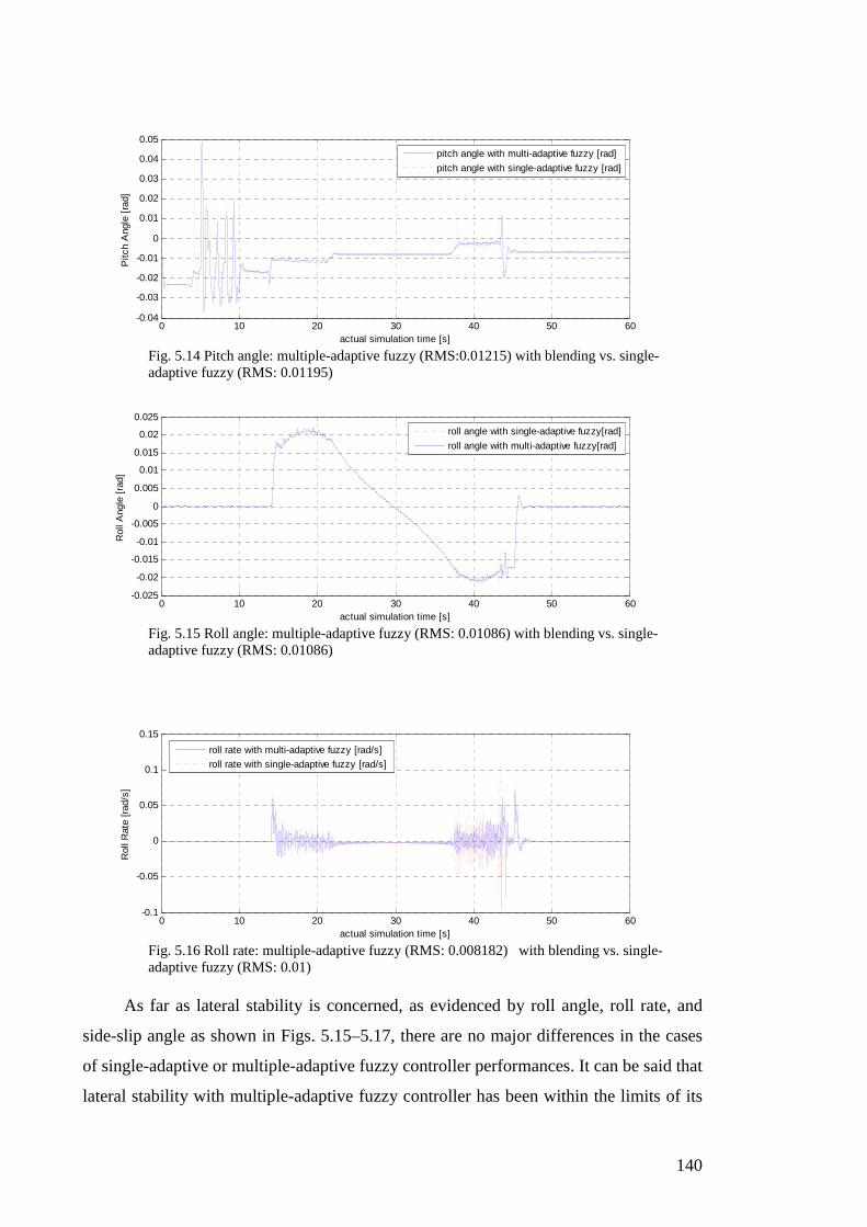
140
0 10 20 30 40 50 60-0.04
-0.03
-0.02
-0.01
0
0.01
0.02
0.03
0.04
0.05
actual simulation time [s]
Pitc
h A
ngle
[ra
d]
pitch angle with multi-adaptive fuzzy [rad]
pitch angle with single-adaptive fuzzy [rad]
Fig. 5.14 Pitch angle: multiple-adaptive fuzzy (RMS:0.01215) with blending vs. single-adaptive fuzzy (RMS: 0.01195)
0 10 20 30 40 50 60-0.025
-0.02
-0.015
-0.01
-0.005
0
0.005
0.01
0.015
0.02
0.025
actual simulation time [s]
Rol
l Ang
le [
rad]
roll angle with single-adaptive fuzzy[rad]
roll angle with multi-adaptive fuzzy[rad]
Fig. 5.15 Roll angle: multiple-adaptive fuzzy (RMS: 0.01086) with blending vs. single-adaptive fuzzy (RMS: 0.01086)
0 10 20 30 40 50 60-0.1
-0.05
0
0.05
0.1
0.15
actual simulation time [s]
Rol
l Rat
e [r
ad/s
]
roll rate with multi-adaptive fuzzy [rad/s]
roll rate with single-adaptive fuzzy [rad/s]
Fig. 5.16 Roll rate: multiple-adaptive fuzzy (RMS: 0.008182) with blending vs. single-adaptive fuzzy (RMS: 0.01)
As far as lateral stability is concerned, as evidenced by roll angle, roll rate, and
side-slip angle as shown in Figs. 5.15–5.17, there are no major differences in the cases
of single-adaptive or multiple-adaptive fuzzy controller performances. It can be said that
lateral stability with multiple-adaptive fuzzy controller has been within the limits of its
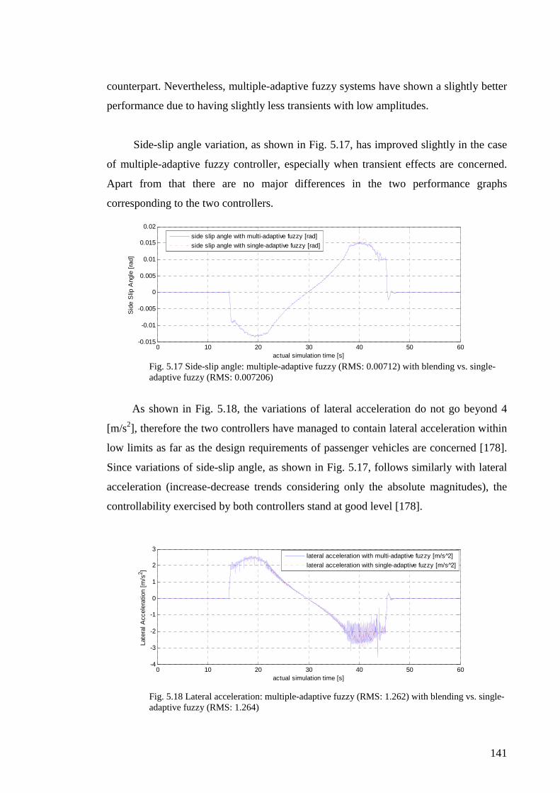
141
counterpart. Nevertheless, multiple-adaptive fuzzy systems have shown a slightly better
performance due to having slightly less transients with low amplitudes.
Side-slip angle variation, as shown in Fig. 5.17, has improved slightly in the case
of multiple-adaptive fuzzy controller, especially when transient effects are concerned.
Apart from that there are no major differences in the two performance graphs
corresponding to the two controllers.
0 10 20 30 40 50 60-0.015
-0.01
-0.005
0
0.005
0.01
0.015
0.02
actual simulation time [s]
Sid
e S
lip A
ngle
[ra
d]
side slip angle with multi-adaptive fuzzy [rad]
side slip angle with single-adaptive fuzzy [rad]
Fig. 5.17 Side-slip angle: multiple-adaptive fuzzy (RMS: 0.00712) with blending vs. single-adaptive fuzzy (RMS: 0.007206)
As shown in Fig. 5.18, the variations of lateral acceleration do not go beyond 4
[m/s2], therefore the two controllers have managed to contain lateral acceleration within
low limits as far as the design requirements of passenger vehicles are concerned [178].
Since variations of side-slip angle, as shown in Fig. 5.17, follows similarly with lateral
acceleration (increase-decrease trends considering only the absolute magnitudes), the
controllability exercised by both controllers stand at good level [178].
0 10 20 30 40 50 60-4
-3
-2
-1
0
1
2
3
actual simulation time [s]
Late
ral A
ccel
erat
ion
[m/s
2 ]
lateral acceleration with multi-adaptive fuzzy [m/s 2]
lateral acceleration with single-adaptive fuzzy [m/s 2]
Fig. 5.18 Lateral acceleration: multiple-adaptive fuzzy (RMS: 1.262) with blending vs. single-adaptive fuzzy (RMS: 1.264)

142
Overall, under normal cruising conditions, the multiple-adaptive fuzzy controller
has shown good tracking both in lateral and longitudinal aspects in comparison to the
single-adaptive fuzzy controller. As evidenced by variations of side-slip angle, roll-
angle and roll rate, lateral stability of multiple-adaptive fuzzy system stands at a good
level in comparison to the performances of its counterpart. In other words, while
multiple-adaptive fuzzy controller shows good lateral and longitudinal tracking
performance in comparison to its counterpart, it shows a level of lateral stability at least
similar to that with its counterpart—this is a good performance.
(b) External Disturbances: Multiple-Adaptive Fuzzy Control with Blending
In the following set of simulations, the developed multiple-adaptive fuzzy
controller was tested against the single-adaptive fuzzy controller under a number of
external disturbances. These disturbances included an unsymmetrical load mass on the
vehicle, presence of crosswind forces, and change of tyre-road friction.
1. Unsymmetrical Load Mass
The following simulation was carried out for the comparison of results between
the multiple-adaptive fuzzy controller and the single-adaptive fuzzy controller, when
there was an unsymmetrical load-mass on the vehicle as per the details described in
Section 3.2.18.
As shown in Fig. 5.19, longitudinal error with the multiple-adaptive fuzzy
controller is slightly less initially (approximately around 8 [s] on the time-scale) against
that of the single-adaptive fuzzy controller. The peak value around 20 – 25 [s] is due to
a sudden change of curvature with increasing speed.

143
0 10 20 30 40 50 60-5
0
5
10
15
20
actual simulation time [s]
Long
itudi
nal E
rror
[m
]
longitudinal error with single-adaptive fuzzy [m]
longitudinal error with multiple-adaptive fuzzy with blending [m]
Fig. 5.19 Longitudinal error: multiple-adaptive fuzzy with blending (RMS: 4.347) vs. single-adaptive fuzzy (RMS: 4.391)
Lateral error, as shown in Fig. 5.20, has been reduced with the multiple-adaptive
fuzzy controller throughout as compared to that with the single-adaptive fuzzy
controller. Especially, diminishing of transient effects can be seen throughout with the
reduction of the amplitudes of chattering.
0 10 20 30 40 50 60-0.01
-0.005
0
0.005
0.01
0.015
0.02
actual simulation time [s]
Late
ral E
rror
[m
]
lateral error with single-adaptive fuzzy [m]
lateral error with multiple-adaptive fuzzywith blending [m]
Fig. 5.20 Lateral error: multiple-adaptive fuzzy with blending (RMS: 0.002075) vs. single-adaptive fuzzy (RMS: 0.003957)
0 10 20 30 40 50 60-0.05
-0.04
-0.03
-0.02
-0.01
0
0.01
0.02
actual simulation time [s]
Pitc
h A
ngle
[ra
d]
pitch angle with multiple-adaptive fuzzy with blending [rad]
pitch angle with single-adaptive fuzzy [rad]
Fig. 5.21 Pitch angle: multiple-adaptive fuzzy with blending (RMS: 0.02004) vs. single-adaptive fuzzy (RMS: 0.01998)

144
0 10 20 30 40 50 60-0.04
-0.035
-0.03
-0.025
-0.02
-0.015
-0.01
-0.005
0
0.005
0.01
actual simulation time [s]
Rol
l Ang
le [
rad]
roll angle with multiple-adaptive fuzzy with blending [rad]
roll angle with single-adaptive fuzzy [rad]
Fig. 5.22 Roll angle: multiple-adaptive fuzzy with blending (RMS: 0.01766) vs. single-adaptive fuzzy (RMS: 0.01766)
0 10 20 30 40 50 60-0.1
-0.08
-0.06
-0.04
-0.02
0
0.02
0.04
0.06
0.08
0.1
actual simulation time [s]
Rol
l Rat
e [r
ad/s
]
roll rate with multiple-adaptive fuzzy with blending [rad/s]
roll rate with single-adaptive fuzzy [rad/s]
Fig. 5.23 Roll rate: multiple-adaptive fuzzy with blending (RMS: 0.0114) vs. single-adaptive fuzzy (RMS: 0.015)
0 10 20 30 40 50 60-0.04
-0.03
-0.02
-0.01
0
0.01
0.02
actual simulation time [s]
Sid
e-S
lip A
ngle
[ra
d]
side-slip angle with multiple-adaptive fuzzy with blending [rad]
side-slip angle with single-adaptive fuzzy [rad]
Fig. 5.24 Side-slip angle: multiple-adaptive fuzzy with blending (RMS: 0.008215) vs. single-adaptive fuzzy (RMS: 0.008237)
Variations of roll angle, roll rate and side-slip angle throughout the simulation
have been slightly on the low side with the multiple-adaptive fuzzy controller.
Therefore, it has performed slightly better (due to reduction in transient effects) in
comparison to the single-adaptive fuzzy controller. This suggests lateral stability with
multiple-adaptive fuzzy controller is slightly better. These parameter changes are
illustrated in Figs. 5.22–5.24.
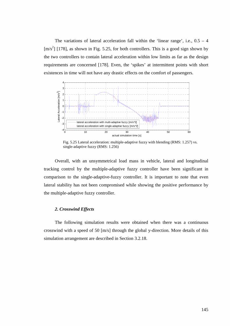
145
The variations of lateral acceleration fall within the ‘linear range’, i.e., 0.5 – 4
[m/s2] [178], as shown in Fig. 5.25, for both controllers. This is a good sign shown by
the two controllers to contain lateral acceleration within low limits as far as the design
requirements are concerned [178]. Even, the ‘spikes’ at intermittent points with short
existences in time will not have any drastic effects on the comfort of passengers.
0 10 20 30 40 50 60-4
-3
-2
-1
0
1
2
3
4
actual simulation time [s]
Late
ral A
ccel
erat
ion
[m/s
2 ]
lateral acceleration with multi-adaptive fuzzy [m/s 2]
lateral acceleration with single-adaptive fuzzy [m/s 2]
Fig. 5.25 Lateral acceleration: multiple-adaptive fuzzy with blending (RMS: 1.257) vs. single-adaptive fuzzy (RMS: 1.256)
Overall, with an unsymmetrical load mass in vehicle, lateral and longitudinal
tracking control by the multiple-adaptive fuzzy controller have been significant in
comparison to the single-adaptive-fuzzy controller. It is important to note that even
lateral stability has not been compromised while showing the positive performance by
the multiple-adaptive fuzzy controller.
2. Crosswind Effects
The following simulation results were obtained when there was a continuous
crosswind with a speed of 50 [m/s] through the global y-direction. More details of this
simulation arrangement are described in Section 3.2.18.

146
0 10 20 30 40 50 60-5
0
5
10
15
20
actual simulation time [s]
Long
itudi
nal E
rror
[m
]
longitudinal error with single-adaptive fuzzy [m]
longitudinal error with multi-adaptive fuzzy [m]
Fig. 5.26 Longitudinal error: multiple-adaptive fuzzy with blending (RMS: 3.658) vs. single-adaptive fuzzy (RMS: 3.742)
0 10 20 30 40 50 60-0.02
-0.01
0
0.01
0.02
0.03
0.04
actual simulation time [s]
Late
ral E
rror
[m
]
lateral error with multi-adaptive fuzzy [m]
lateral error with single-adaptive fuzzy [m]
Fig. 5.27 Lateral error: multiple-adaptive fuzzy with blending (RMS: 0.003626) vs. single-adaptive fuzzy (RMS: 0.005914)
Once again, longitudinal and lateral tracking performances of multiple-adaptive
fuzzy controller have been significantly better than that of the single-adaptive fuzzy
controller, as shown in Figs. 5.26–5.27. Especially with lateral tracking, transient errors
have been mostly suppressed throughout by the multiple-adaptive fuzzy controller as
against that by the single-adaptive fuzzy controller.

147
0 10 20 30 40 50 60-0.04
-0.03
-0.02
-0.01
0
0.01
0.02
0.03
actual simulation time [s]
Pitc
h A
ngle
[ra
d]
pitch angle with multiple-adaptive fuzzy with blending [rad]
pitch angle with single-adaptive fuzzy [rad]
Fig. 5.28 Pitch angle: multiple-adaptive fuzzy with blending (RMS: 0.01146) vs. single-adaptive fuzzy (RMS: 0.01142)
0 10 20 30 40 50 60-0.04
-0.03
-0.02
-0.01
0
0.01
0.02
actual simulation time [s]
Rol
l Ang
le [
rad]
roll angle with multiple-adaptive fuzzy with blending [rad]
roll angle with single-adaptive fuzzy [rad]
Fig. 5.29 Roll angle: multiple-adaptive fuzzy with blending (RMS:0.01399) vs. single-adaptive fuzzy (RMS: 0.01396)
0 10 20 30 40 50 60-0.15
-0.1
-0.05
0
0.05
0.1
0.15
0.2
0.25
actual simulation time [s]
Rol
l Rat
e [r
ad/s
]
roll rate with multiple-adaptive fuzzy with blending [rad/s]
roll rate with single-adaptive fuzzy [rad/s]
Fig. 5.30 Roll rate: multiple-adaptive fuzzy with blending (RMS: 0.01223) vs. single-adaptive fuzzy (RMS: 0.02222)

148
0 10 20 30 40 50 60-0.03
-0.02
-0.01
0
0.01
0.02
0.03
0.04
actual simulation time [s]
Sid
e-S
lip A
ngle
[ra
d]
side-slip angle with multiple-adaptive fuzzy with blending [rad]
side-slip angle with single-adaptive fuzzy [rad]
Fig. 5.31 Side-slip angle: multiple-adaptive fuzzy with blending (RMS:0.01449) vs. single-adaptive fuzzy (RMS: 0.01438)
As shown by variations of roll angle, roll rate and side-slip angles, lateral stability
has been maintained to a consistent level by the multiple-adaptive fuzzy controller. This
level of lateral stability is almost in par with that of the single-adaptive fuzzy controller.
These performances are shown in Figs. 5.29–5.31. Nevertheless, there are some slight
over reactions by the multiple-adaptive fuzzy controllers, too, e.g. with side-slip angle
during 5–10 [s] on the time-scale in Fig. 5.31. Since these variations are not excessive,
they do not threaten lateral stability of the vehicle.
As shown in Fig. 5.28, pitch angle variations have been consistent with each
controller, and therefore the longitudinal stability has been maintained with both
controllers.
As shown in Fig. 5.32, the variation of lateral acceleration with the multiple-
adaptive fuzzy controller has been slightly in excess over 4 [m/s2] around the point 42
[s] on the time-scale. This is said to be just above the ‘linear range’, and therefore
slightly in the so called ‘transition stage’ [178]. Since the effective time period in
relation to the slightly excessive values is quite limited, the effects felt on the vehicle
are quite small. Therefore, the lateral acceleration variation as shown for the multiple-
adaptive fuzzy controller is still acceptable.

149
0 10 20 30 40 50 60-5
-4
-3
-2
-1
0
1
2
3
actual simulation time [s]
Late
ral A
ccel
erat
ion
[m/s
2 ]
lateral acceleration with multiple-adaptive fuzzy with blending [m/s 2]
lateral acceleration with single-adaptive fuzzy [m/s 2]
Fig. 5.32 Lateral acceleration: multiple-adaptive fuzzy with blending (RMS: 1.27) vs. single-adaptive fuzzy (RMS: 1.285)
Overall, in the presence of crosswind effects, the lateral and longitudinal tracking
established by the multiple-adaptive fuzzy controller is satisfactory. Nevertheless,
lateral stability specifically in the areas of side-slip angle, roll-angle and roll rate, has
shown some slight lapses in initial periods. But, these lapses are not excessive and
should be considered against the gains from the improved lateral tracking.
3. Tyre-Road Friction Change
The following simulation results show the performance of the multiple-adaptive
fuzzy controllers compared against the single-adaptive fuzzy controller when there was
a change of tyre-road friction in the range 100–200 [m], on the highway.
As shown in Figs. 5.33–5.34, longitudinal and lateral tracking performances with
the multiple-adaptive fuzzy controller are better than that with the single-adaptive fuzzy
controller.
0 10 20 30 40 50 60-2
0
2
4
6
8
10
12
14
actual simulation time [s]
Long
itudi
nal E
rror
[m
]
longitudinal error with multiple-adaptive fuzzy with blending [m]
longitudinal error with single-adaptive fuzzy [m]
Fig. 5.33 Longitudinal error: multiple-adaptive fuzzy with blending (RMS: 3.077) vs. single-adaptive fuzzy (RMS: 3.158)

150
0 10 20 30 40 50 60-0.02
-0.015
-0.01
-0.005
0
0.005
0.01
0.015
actual simulation time [s]
Late
ral E
rror
[m
]
lateral error with multiple-adaptive fuzzy with blending [m]
lateral error with single-adaptive fuzzy [m]
Fig. 5.34 Lateral error: multiple-adaptive fuzzy with blending (RMS: 0.002091) vs. single-adaptive fuzzy (RMS: 0.003996)
The two controllers fared similarly on variation of pitch angle, except for a high
‘spike’ by the multiple-adaptive fuzzy controller towards the point 5 [s] on the time-
scale. This is shown in Fig. 5.35 below.
0 10 20 30 40 50 60-0.04
-0.03
-0.02
-0.01
0
0.01
0.02
0.03
0.04
0.05
actual simulation time [s]
Pitc
h A
ngle
[ra
d]
pitch angle with multiple-adaptive fuzzy with blending [rad]
pitch angle with single-adaptive fuzzy [rad]
Fig. 5.35 Pitch angle: multiple-adaptive fuzzy with blending (RMS: 0.01162) vs. single-adaptive fuzzy (RMS: 0.01144)
0 10 20 30 40 50 60-0.025
-0.02
-0.015
-0.01
-0.005
0
0.005
0.01
0.015
0.02
0.025
actual simulation time [s]
Rol
l Ang
le [
rad]
roll angle with multiple-adaptive fuzzy with blending [rad]
roll angle with single-adaptive fuzzy [rad]
Fig. 5.36 Roll angle: multiple-adaptive fuzzy with blending (RMS: 0.01086) vs. single-adaptive fuzzy (RMS: 0.01085)

151
0 10 20 30 40 50 60-0.1
-0.05
0
0.05
0.1
0.15
actual simulation time [s]
Rol
l Rat
e [r
ad/s
]
roll rate with multiple-adaptive fuzzy with blending [rad/s]
roll rate with single-adaptive fuzzy [rad/s]
Fig. 5.37 Roll rate: multiple-adaptive fuzzy with blending (RMS: 0.01036) vs. single-adaptive fuzzy (RMS: 0.01255)
0 10 20 30 40 50 60-0.015
-0.01
-0.005
0
0.005
0.01
0.015
0.02
actual simulation time [s]
Sid
e S
lip A
ngle
[ra
d]
side slip angle with multiple-adaptive fuzzy with blending [rad]
side slip angle with single-adaptive fuzzy [rad]
Fig. 5.38 Side-slip angle: multiple-adaptive fuzzy with blending (RMS: 0.007171) vs. single-adaptive fuzzy (RMS: 0.007268)
The variations of roll angle, roll rate and side-slip angle as shown in Figs. 5.36–
5.38, indicate that lateral stability has been quite consistent with both types of
controllers.
The variation of lateral acceleration, as shown in Fig. 5.39, with the multiple-
adaptive fuzzy controllers has almost been below 4 [m/s2] limit [178], except for a slight
‘spike’ at around 41 [s] on the time-scale. Therefore, it suggests that the multiple-
adaptive fuzzy controllers have ensured that lateral acceleration is almost below the
limit ensured by design requirements [178]. The only exception to the limit is quite
negligible since it is not overly excessive and the duration of the spike is quite small.

152
0 10 20 30 40 50 60-5
-4
-3
-2
-1
0
1
2
3
actual simulation time [s]
Late
ral A
ccel
erat
ion
[m/s
2 ]
lateral acceleration with multiple-adaptive fuzzy with blending [m/s 2]
lalateral acceleration with single-adaptive fuzzy [m/s 2]
Fig. 5.39 Lateral acceleration: multiple-adaptive fuzzy with blending (RMS: 1.264) vs. single-adaptive fuzzy (RMS: 1.266)
Overall, in the presence of tyre-road friction changes, the lateral and longitudinal
tracking performances have been impressive as shown with the multiple-adaptive fuzzy
controller in comparison to the single-adaptive-fuzzy controller. These good
performances have been ensured by good lateral stability as suggested by side-slip
angle, roll angle and roll-rate.
(c) Failure Modes (non-catastrophic subsystem failures): Multiple-Adaptive Fuzzy Control with Blending
The following simulation results compare the performance of the multiple-
adaptive fuzzy controllers with blending against that of the single-adaptive fuzzy
controller when some failures in the vehicle components occur. The failures considered
in this simulation included a flat-tyre in the front-left tyre, and a 90% drop of pressure
in the brake line of the front-left wheel cylinder of the vehicle.
1. Flat-Tyre
The following simulation results were obtained when an event of flat-tyre in the
front-left wheel occured at 10[s], after starting the simulation. The details of the
simulation arrangement is explained in Section 3.2.18
As shown in Fig. 5.40, the longitudinal tracking performance with the multiple-
adaptive fuzzy controller is slightly better than that with the single-adaptive fuzzy
controller.
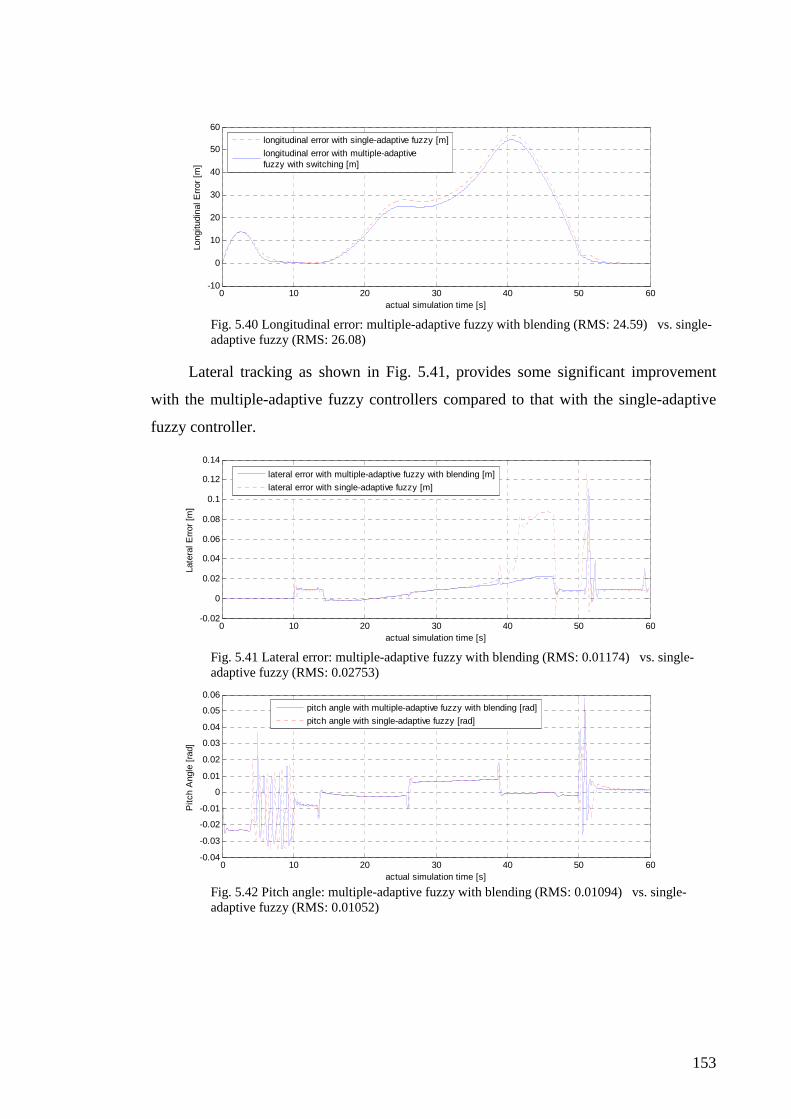
153
0 10 20 30 40 50 60-10
0
10
20
30
40
50
60
actual simulation time [s]
Long
itudi
nal E
rror
[m
]
longitudinal error with single-adaptive fuzzy [m]
longitudinal error with multiple-adaptivefuzzy with switching [m]
Fig. 5.40 Longitudinal error: multiple-adaptive fuzzy with blending (RMS: 24.59) vs. single-adaptive fuzzy (RMS: 26.08)
Lateral tracking as shown in Fig. 5.41, provides some significant improvement
with the multiple-adaptive fuzzy controllers compared to that with the single-adaptive
fuzzy controller.
0 10 20 30 40 50 60-0.02
0
0.02
0.04
0.06
0.08
0.1
0.12
0.14
actual simulation time [s]
Late
ral E
rror
[m
]
lateral error with multiple-adaptive fuzzy with blending [m]
lateral error with single-adaptive fuzzy [m]
Fig. 5.41 Lateral error: multiple-adaptive fuzzy with blending (RMS: 0.01174) vs. single-adaptive fuzzy (RMS: 0.02753)
0 10 20 30 40 50 60-0.04
-0.03
-0.02
-0.01
0
0.01
0.02
0.03
0.04
0.05
0.06
actual simulation time [s]
Pitc
h A
ngle
[ra
d]
pitch angle with multiple-adaptive fuzzy with blending [rad]
pitch angle with single-adaptive fuzzy [rad]
Fig. 5.42 Pitch angle: multiple-adaptive fuzzy with blending (RMS: 0.01094) vs. single-adaptive fuzzy (RMS: 0.01052)
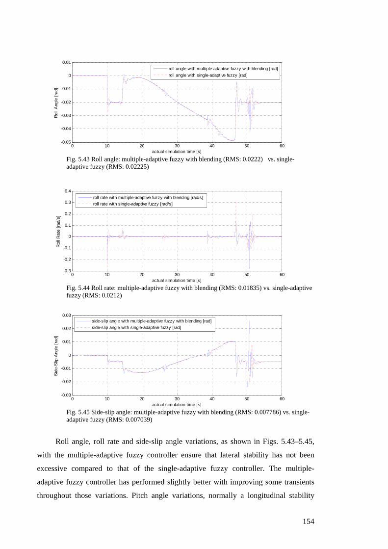
154
0 10 20 30 40 50 60-0.05
-0.04
-0.03
-0.02
-0.01
0
0.01
actual simulation time [s]
Rol
l Ang
le [
rad]
roll angle with multiple-adaptive fuzzy with blending [rad]
roll angle with single-adaptive fuzzy [rad]
Fig. 5.43 Roll angle: multiple-adaptive fuzzy with blending (RMS: 0.0222) vs. single-adaptive fuzzy (RMS: 0.02225)
0 10 20 30 40 50 60-0.3
-0.2
-0.1
0
0.1
0.2
0.3
0.4
actual simulation time [s]
Rol
l Rat
e [r
ad/s
]
roll rate with multiple-adaptive fuzzy with blending [rad/s]
roll rate with single-adaptive fuzzy [rad/s]
Fig. 5.44 Roll rate: multiple-adaptive fuzzy with blending (RMS: 0.01835) vs. single-adaptive fuzzy (RMS: 0.0212)
0 10 20 30 40 50 60-0.03
-0.02
-0.01
0
0.01
0.02
0.03
actual simulation time [s]
Sid
e-S
lip A
ngle
[ra
d]
side-slip angle with multiple-adaptive fuzzy with blending [rad]
side-slip angle with single-adaptive fuzzy [rad]
Fig. 5.45 Side-slip angle: multiple-adaptive fuzzy with blending (RMS: 0.007786) vs. single-adaptive fuzzy (RMS: 0.007039)
Roll angle, roll rate and side-slip angle variations, as shown in Figs. 5.43–5.45,
with the multiple-adaptive fuzzy controller ensure that lateral stability has not been
excessive compared to that of the single-adaptive fuzzy controller. The multiple-
adaptive fuzzy controller has performed slightly better with improving some transients
throughout those variations. Pitch angle variations, normally a longitudinal stability
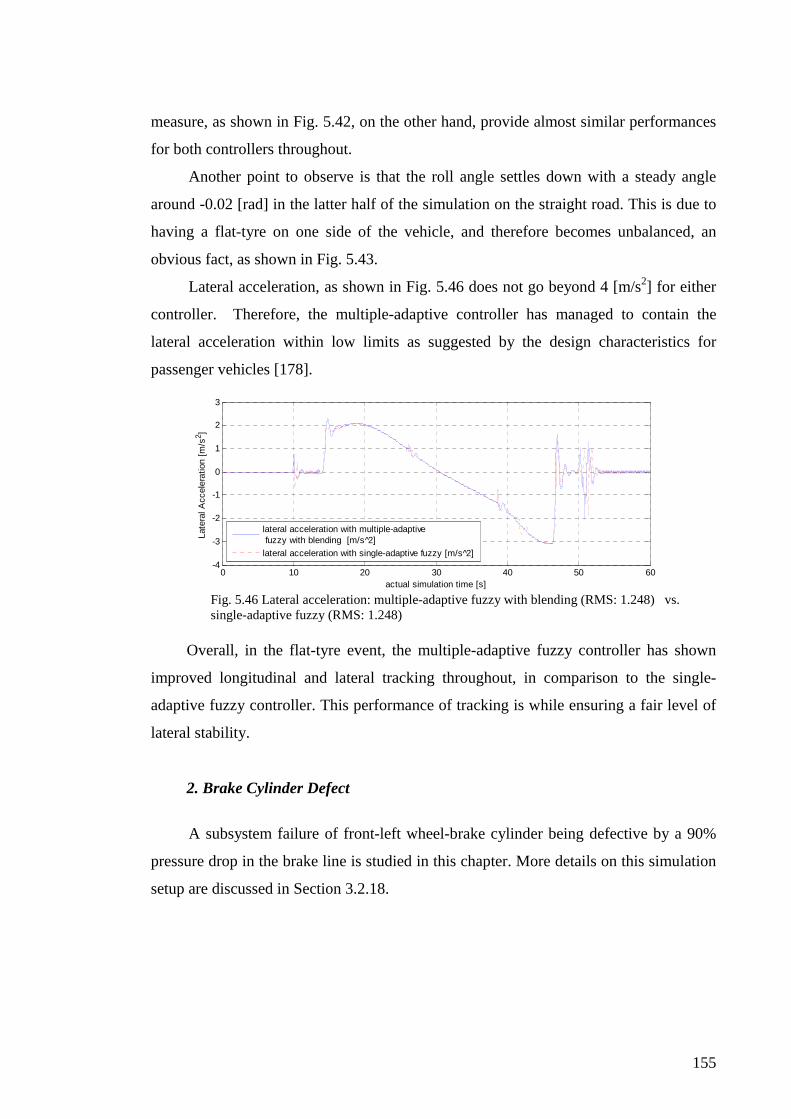
155
measure, as shown in Fig. 5.42, on the other hand, provide almost similar performances
for both controllers throughout.
Another point to observe is that the roll angle settles down with a steady angle
around -0.02 [rad] in the latter half of the simulation on the straight road. This is due to
having a flat-tyre on one side of the vehicle, and therefore becomes unbalanced, an
obvious fact, as shown in Fig. 5.43.
Lateral acceleration, as shown in Fig. 5.46 does not go beyond 4 [m/s2] for either
controller. Therefore, the multiple-adaptive controller has managed to contain the
lateral acceleration within low limits as suggested by the design characteristics for
passenger vehicles [178].
0 10 20 30 40 50 60-4
-3
-2
-1
0
1
2
3
actual simulation time [s]
Late
ral A
ccel
erat
ion
[m/s
2 ]
lateral acceleration with multiple-adaptive fuzzy with blending [m/s 2]
lateral acceleration with single-adaptive fuzzy [m/s 2]
Fig. 5.46 Lateral acceleration: multiple-adaptive fuzzy with blending (RMS: 1.248) vs. single-adaptive fuzzy (RMS: 1.248)
Overall, in the flat-tyre event, the multiple-adaptive fuzzy controller has shown
improved longitudinal and lateral tracking throughout, in comparison to the single-
adaptive fuzzy controller. This performance of tracking is while ensuring a fair level of
lateral stability.
2. Brake Cylinder Defect
A subsystem failure of front-left wheel-brake cylinder being defective by a 90%
pressure drop in the brake line is studied in this chapter. More details on this simulation
setup are discussed in Section 3.2.18.

156
0 10 20 30 40 50 60-2
0
2
4
6
8
10
12
14
actual simulation time [s]
Long
itudi
nal E
rror
[m
]
longitudinal error with multiple-adaptive fuzzy with blending [m]
longitudinal error with single-adaptive fuzzy [m]
Fig. 5.47 Longitudinal error: multiple-adaptive fuzzy with blending (RMS: 3.064) vs. single-adaptive fuzzy (RMS: 3.159)
0 10 20 30 40 50 60-0.1
0
0.1
0.2
0.3
0.4
actual simulation time [s]
Late
ral E
rror
[m
]
lateral error with single-adaptive fuzzy [m]
lateral error with multiple-adaptive fuzzy with blending [m]
Fig. 5.48 Lateral error: multiple-adaptive fuzzy with blending (RMS: 0.02501) vs. single-adaptive fuzzy (RMS: 0.03453)
As shown in Figs. 5.47–5.48, the multiple-adaptive fuzzy controller has shown
significant improvements in both types of tracking, i.e. lateral and longitudinal.
Pitch angle variations, normally a measure for longitudinal stability, as shown in
Fig. 5.49 provide similar performances for both controllers.
0 10 20 30 40 50 60-0.05
-0.04
-0.03
-0.02
-0.01
0
0.01
0.02
0.03
0.04
actual simulation time [s]
Pitc
h A
ngle
[ra
d]
pitch angle with multiple-adaptive fuzzy with blending [rad]
pitch angle with single-adaptive fuzzy [rad]
Fig. 5.49 Pitch angle: multiple-adaptive fuzzy with blending (RMS: 0.01437) vs. single-adaptive fuzzy (RMS: 0.01583)
As shown in Fig. 5.50, as far as roll angle is concerned, the two controllers show
performances with some inconsistency, i.e., during some time intervals multiple-

157
adaptive controller has done well, e.g., 38 – 43 [s], while during other time intervals
single-adaptive fuzzy controller has done better, e.g., 16 – 17 [s]. Therefore, it is
difficult to compare one controller against the other in this regard. Therefore, it can be
said that the performance of the multiple-adaptive fuzzy controllers is acceptable
compared to the single-adaptive fuzzy controller as far as lateral stability is concerned.
0 10 20 30 40 50 60-0.04
-0.03
-0.02
-0.01
0
0.01
0.02
0.03
0.04
actual simulation time [s]
Rol
l Ang
le [
rad]
roll angle with multiple-adaptive fuzzy with blending [rad]
roll angle with single-adaptive fuzzy [rad]
Fig. 5.50 Roll angle: multiple-adaptive fuzzy with blending (RMS: 0.01078) vs. single-adaptive fuzzy (RMS: 0.01082)
When the variation of roll rate, as shown in Fig. 5.51, is considered, the multiple-
adaptive fuzzy controller has shown some significant improvements over its counterpart
during high-values, e.g. 37–43 [s], but during periods with lower values of roll-rate, the
single-adaptive fuzzy controller has outperformed its counterpart, e.g. throughout 22 –
37 [s], 47 –60 [s].
0 10 20 30 40 50 60-0.4
-0.3
-0.2
-0.1
0
0.1
0.2
0.3
0.4
actual simulation time [s]
Rol
l Rat
e [r
ad/s
]
roll rate with multiple-adaptive fuzzy with blending [rad/s]
roll rate with single-adaptive fuzzy [rad/s]
Fig. 5.51 Roll rate: multiple-adaptive fuzzy with blending (RMS: 0.03665) vs. single-adaptive fuzzy (RMS: 0.04617)
Side-slip angle variations as shown in Fig. 5.52, have been similar most the time
throughout, while multiple-adaptive fuzzy controller has shown some improvements
compared to its counterpart over transients, i.e. especially during 5–10 [s] and 38–43
[s].

158
0 10 20 30 40 50 60-0.08
-0.06
-0.04
-0.02
0
0.02
0.04
actual simulation time [s]
Sid
e-S
lip A
ngle
[ra
d]
side-slip angle with multiple-adaptive fuzzy with blending [rad]
side-slip angle with single-adaptive fuzzy [rad]
Fig. 5.52 Side-slip angle: multiple-adaptive fuzzy with blending (RMS: 0.009008) vs. single-adaptive fuzzy (RMS: 0.01052)
Considering Figs. 5.50–5.52, on roll angle, roll rate and side-slip angle, it can be
said that the multiple-adaptive fuzzy controller ensures a fairly good level of lateral
stability in comparison to the single-adaptive controller.
As shown in Fig. 5.53, lateral acceleration for the multiple-adaptive fuzzy
controller does not go beyond 4 [m/s2]. This is a good performance in comparison to
some other performances by the single-adaptive fuzzy controller as shown in Fig. 5.53.
Therefore, the multiple-adaptive fuzzy controller has performed well to contain the
lateral acceleration within low limits as suggested by design requirements for passenger
vehicles [178].
0 10 20 30 40 50 60-20
-15
-10
-5
0
5
10
actual simulation time [s]
Late
ral A
ccel
erat
ion
[m/s
2 ]
lateral acceleration with multiple-adaptive fuzzy with blending [m/s 2]
lateral acceleration with single-adaptive fuzzy [m/s 2]
Fig. 5.53 Lateral acceleration: multiple-adaptive fuzzy with blending (RMS: 1.819) vs. single-adaptive fuzzy (RMS: 1.334)
Overall, in the presence of a wheel brake cylinder failure, the multiple-adaptive
fuzzy controller has managed to ensure a good level of lateral and longitudinal tracking
performance in comparison to the single-adaptive fuzzy controller. These results have
been achieved in the presence of a good level of lateral stability.
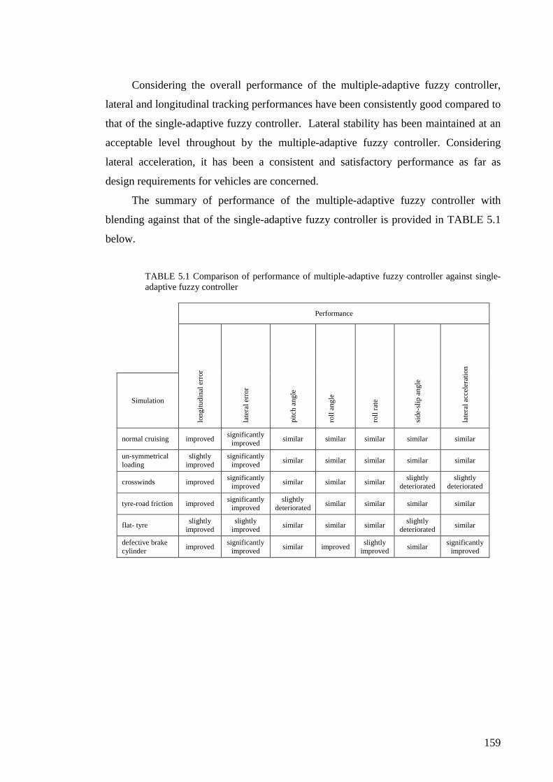
159
Considering the overall performance of the multiple-adaptive fuzzy controller,
lateral and longitudinal tracking performances have been consistently good compared to
that of the single-adaptive fuzzy controller. Lateral stability has been maintained at an
acceptable level throughout by the multiple-adaptive fuzzy controller. Considering
lateral acceleration, it has been a consistent and satisfactory performance as far as
design requirements for vehicles are concerned.
The summary of performance of the multiple-adaptive fuzzy controller with
blending against that of the single-adaptive fuzzy controller is provided in TABLE 5.1
below.
TABLE 5.1 Comparison of performance of multiple-adaptive fuzzy controller against single-adaptive fuzzy controller
Performance
Simulation
long
itudi
nal e
rror
late
ral e
rror
pitc
h a
ngle
roll
ang
le
roll
rate
side
-slip
ang
le
late
ral a
cce
lera
tion
normal cruising improved significantly
improved similar similar similar similar similar
un-symmetrical loading
slightly improved
significantly improved
similar similar similar similar similar
crosswinds improved significantly
improved similar similar similar
slightly deteriorated
slightly deteriorated
tyre-road friction improved significantly
improved slightly
deteriorated similar similar similar similar
flat- tyre slightly
improved slightly
improved similar similar similar slightly
deteriorated similar
defective brake cylinder
improved significantly
improved similar improved
slightly improved
similar significantly
improved
160
5.2 Robust Multiple-Model Fuzzy PDC-based Multiple-Adaptive Fuzzy Control System - Blending (Soft - Switching)
5.2.1 Introduction
As explained in the main introduction, there are drawbacks in using single-model
(or single ‘modal’) control systems for addressing the problem of integrated lateral and
longitudinal control of highway vehicles.
Multiple-Model/Multiple-Controller (MM/MC) systems have more built-in
capability to address control requirements with improved tracking, and therefore are
more suitable in an Automated Highway System (AHS) environment.
In this section, the design of a fuzzy PDC (Parallel Distributed Compensation)
based multiple-adaptive fuzzy controller (as a multiple-model control method) is
described. The MM/MC system designed in this section is to address the problem of
integrated lateral and longitudinal control of highway vehicles. This novel design of
fuzzy PDC system provides an effective MM/MC setup since it improves versatility of
the system with the inclusion of nonlinear adaptive fuzzy controllers. In most of the
previous PDC based fuzzy systems, local linear models and linear controllers were
used. Due to the addition of complex adaptive fuzzy controllers in the control structure,
the scope of the fuzzy PDC based controller has been widened. Therefore, it can
successfully address the multiple-modal characteristics and other nonlinear issues and
complexities of the integrated lateral and longitudinal control problem of vehicles.
Importantly, adaptive fuzzy control functions enable one to define and model
uncertainty of the system over which the control action is developed. The design of the
fuzzy PDC system is based on having ‘state-signals as inputs’ in the fuzzy PDC system.
In the design for implementation of the controller, nonlinear local models are generated
out of the vehicle model (simplified) following the ‘sector nonlinearity’ method.
161
5.2.2 Synthesis of Multiple-Model Fuzzy PDC-based Multiple-Adaptive Fuzzy Controller
This section describes the synthesis of a novel robust fuzzy PDC based multiple-
model/multiple-adaptive fuzzy controller where a number of adaptive fuzzy controllers
are blended using a fuzzy PDC structure to obtain the control function. In the
development of the proposed controller, non-linear local models are used. A parallel set
of adaptive fuzzy controllers are used to address ‘uncertainty’ of the control problem of
integrated lateral and longitudinal control of highway vehicles. In the meantime,
proportional-derivative (PD) control module is used for coarse tracking in the lateral
and longitudinal aspects of the vehicle control problem.
Having adaptive fuzzy controllers in the PDC structure widens the capability of
the control system to handle uncertainty levels. Therefore, the proposed control system
can effectively handle a larger ‘uncertainty’ gap between the real vehicle system and the
models generated from the design process. With the PDC fuzzy blending, the
capabilities of individual adaptive fuzzy controllers are combined to focus on an
enhanced performance.
(i) Design of Robust Fuzzy PDC Multiple-Model/Multiple-Adaptive Fuzzy Control System
In this PDC system, there is no limitation in the number of local models that can
be included, therefore the relevant number of adaptive fuzzy controllers. It is clear that
both the number of models and adaptive fuzzy controllers are based on the number of
IF-THEN rules used in the PDC fuzzy system.
Let the IF-THEN rules of the fuzzy PDC (Parallel Distributed Compensation) system
(A T–S fuzzy system) be
1R : If 1( )f e is 1
qF AND 2( )f e is 1
rF THEN ( )1 1 1 1x h q b u d= + +ɺɺ ɺ
⋮ ⋮ (5.42)

162
nR :
If 1( )f e is qnF AND 2( )f e is r
nF THEN ( )n n n nx h q b u d= + +ɺɺ ɺ
where ( )jh qɺ , 1, ,j n= ⋯ are true localized dynamics of the vehicle. Here, n is the
number of IF-THEN rules in the fuzzy PDC structure.
1( )f e and 2( )f e are state-based functions in n IF-THEN rules (n number of localized
dynamics for n modes of operations). For example, 1( )f e can be considered as a
longitudinal velocity based function, and 2( )f e can be considered as a lateral velocity
based function.
Let the fuzzy inference from each fuzzy input function of the PDC be
i
jAµ where
1, ,i m= ⋯ (it is taken as 2m= in this design), and 1, ,j n= ⋯ . n is the number of
fuzzy IF-THEN rules. Thereby the T–S fuzzy logic output with product inference,
singleton fuzzifier and centre-average defuzzifier can be expressed as
( ) ( )
( )1
1
11
( )i
i
nm j
A j j j jij
nm j
Aij
h q b u d
x
µ
µ
==
==
+ +=∑ ∏
∑ ∏
ɺ
ɺɺ . (5.43)
Let the normalized regression factor for each rule be
( )
( )1
11
i
i
m jAi
j nm j
Aij
µµ
µ
=
==
=∏
∑ ∏. (5.44)
Then output of the fuzzy PDC system becomes
( )( )1
n
j j j j jjx h q b u dµ
== + +∑ɺɺ ɺ . (5.45)
Let ( )1
( )n
x j jxjq h qρ µ
==∑ɺ ɺ . Thereby the PDC system output as provided in (5.45)
becomes
( )1( )
n
x j j j jjx q b u dρ µ
== + +∑ɺɺ ɺ . (5.46)

163
In the implementation of the fuzzy PDC structure, the schematics of the set of
adaptive fuzzy controllers are provided in Fig. 5.54 below. In this setup, the designed
vehicle model setup has been replaced by the vehicle itself.
Fig. 5.54 Schematic diagram for fuzzy Parallel Distributed Compensation (PDC) scheme for implementation in integrated longitudinal (lateral) control of highway vehicles
(ii) Control Law
The control output from the jth model (using certainty equivalence control law)
for longitudinal case is
1 ˆˆ ( )T
jx p dx x px x j j sx jxx
u x k e k e u h qb = + + + + − ɺɺ ɺ ɺψ θ , (5.47)
and for lateral case is
1 ˆˆ ( )Tjy s dy y py y j j sy jy
y
u l k e k e u h qb
ψ = + + + + − ψ θɺɺɶ ɺ ɺ (5.48)
PD
1µµµµ
nµµµµ
( )1h q− ɺ
( )nh q− ɺ
( )m sx l ɺɶɺ ψ
eɺ
e su
e
( )1f e ( )2f e
d s
t∆∆
1 1Tψ θ
Tn nψ θ
⋮
,1 x yb
+ +
⋮ ⋮
Vehicle
Adaptive Fuzzy Controllers
e ( )∫ i x +
Fuzzy Input Functions
PDC based Fuzzy Control System

164
where 1
n
x j jyjb bµ
==∑ , and
1
n
y j jyjb bµ
==∑ . T
j jψ θ is the jth adaptive fuzzy controller
output. su is the variable structure control term. ˆ ( )jxh qɺ and ˆ ( )jyh qɺ are the longitudinal
and lateral local dynamic models of the vehicle, respectively.
Fuzzy blending of control output from each model in the PDC system will result
in the overall control outputs from the PDC structure as
( ) ( )1 1
1 ˆˆ ,n nT
x p dx x px x j j j sx j jxj jx
u x k e k e u h qb
µ µ= =
= + + + + − ∑ ∑ψ θɺɺ ɺ ɺ (5.49)
( ) ( )1 1
1 ˆˆn nT
y s dy y py y j j j sy j jyj jy
u l k e k e u h qb
ψ µ µ= =
= + + + + − ∑ ∑ɺɺɶ ɺ ɺψ θ (5.50)
for longitudinal and lateral cases, respectively. It is provided that 1
n
x j jxjb bµ
==∑ ,
1
n
y j jyjb bµ
==∑ , and thereby (5.49), (5.50) can be expressed as
( ) ( )1
1ˆˆ ,
n Tx p dx x px x j j j sx xj x
x
u x k e k e u qb
µ ρ=
= + + + + − ∑ ψ θɺɺ ɺ ɺ (5.51)
( ) ( )1
1ˆˆ
n Ty s dy y py y j j j sy yj y
y
u l k e k e u qb
ψ µ ρ=
= + + + + − ∑ ψ θɺɺɶ ɺ ɺ (5.52)
where ( )1
ˆˆ ( )n
x j jxjq h qρ µ
==∑ɺ ɺ and ( )
1ˆˆ ( )
n
y j jyjq h qρ µ
==∑ɺ ɺ .
Remark 5.5: Though fuzzy systems in (5.51), (5.52) are generally nonlinear, each is
linear with respect to its unknown parameters. Hence, parameter adaptation algorithms
applicable for linear systems, e.g. gradient-based algorithms, can be readily used in
estimation of unknown parameters in the fuzzy systems in (5.51), (5.52) [27].
For the jth adaptive fuzzy controller ( 1, ,j n= ⋯ ), the regression vector can be
expressed as 1 2, ,T
j j j jp = ψ ψ ψ ψ⋯ where p is the total number of IF-THEN fuzzy
rules in each adaptive fuzzy controller. The kth element, where 1, ,k p= ⋯ , of the jth
165
controller (where 1, ,j n= ⋯ ) is Tjk jk jk jke eψ ψ ψ = = ψ eɺ . There are p IF-
THEN rules in each adaptive fuzzy controller, i.e. 1, ,k p= ⋯ .
The T–S fuzzy output membership function parameter set of jth adaptive fuzzy
controller can be tuned using an algorithm based on the adaptive law
j j j jγ µ= −θ ψ Ceɺɶ (5.53)
where 1, ,j n= ⋯ .
(iii) Error Dynamics
Substitution of equation (5.51) in (3.4) will result for the longitudinal dynamics
( ) ( ) ( )1
*
ˆ
ˆ( )
,
n Tdx px x x j j j sx xj x
sx x
sx x
e k e k e q q u d
u d
u d
ρ ρ µ
ν τ ν
ν
=+ + = − − − −
= + − − −
= − −
∑ ψ θɺɺ ɺ ɺ ɺ
ɶ
(5.54)
and in the same way, substitution of (5.52) in (3.5) will result for the lateral dynamics
( ) ( ) ( )1
*
ˆ
ˆ( )
n Tdy py y y j j j sy yj y
sy y
sy y
e k e k e q q u d
u d
u d
ρ ρ µ
ν τ ν
ν
=+ + = − − − −
= + − − −
= − −
∑ ψ θɺɺ ɺ ɺ ɺ
ɶ
(5.55)
where ν is the output from the fuzzy PDC system. *ν is the optimum fuzzy PDC
output, and τ is the approximation error of the fuzzy PDC system.
By using the universal approximation theorem (provided in Chapter 4), with the
fuzzy adaptation process, the fuzzy controller parameters can be gradually brought to
the optimal values, and thus the right half of the equations, (5.54) and (5.55) can be
made zero.
166
5.2.3 Robust Stability Analysis of Control System
The following stability proof of the fuzzy PDC multiple-adaptive fuzzy control
system is described for the generic case irrespective whether it is lateral or longitudinal
controller. Therefore, the subscripts that are specific to either longitudinal or lateral case
are removed in this description. Nevertheless, the specific details will be mentioned as
and when necessary.
Assumption 5.2: The sum of fuzzy approximation errors,w is bounded, i.e.,
w W≤ where ( 0)W > ∈R . The external disturbances, d are bounded too, i.e.,
d D≤ where ( 0)D > ∈R . Thereby the variable structure control gain is chosen as
f W Dσ ≥ + .
The main features of the robust multiple-model PDC-based multiple-adaptive
fuzzy controller can be summarized in the following theorem.
Theorem 5.2: Let the parameter vectors, jθ of the adaptive fuzzy systems be adjusted
by the adaptive law as provided in (5.53) and let Assumption 5.2 be true. The proposed
adaptive fuzzy control law as provided in (5.51) [and (5.52)] can guarantee stability of
the vehicle system with the following properties:
i) The closed loop vehicle system is stable, i.e.∈e ∞L (considering both lateral
and longitudinal cases)
ii) The system errors and the parametric errors are asymptotically stable, i.e.
lim 0t x ye , e→∞ = , and lim 0t jθ→∞ =ɶ (considering both lateral and longitudinal
cases) where 1,...,j n= .

167
Proof:
Positive realness of the transfer function of error dynamics equations, i.e., (4.23)
and (4.24), related to vehicle dynamics has already been established in Section 4.2.6.
Assuming that positive realness of the vehicle error dynamics can be established
as shown in Section 4.2.6, according to Kalman–Yakubovich–Popov (KYP) lemma
[175], for a strictly positive real system there exist two positive definite matrices P and
Q (i.e., 0T= >P P and 0T= >Q Q ) satisfying
T + + =A P PA Q 0, and T=PB C . (5.56)
With KYP lemma, the Lyapunov function candidate can be selected as
1
1
nT Tj j jj
V γ −=
= + ∑e Pe θ θɶ ɶ (5.57)
where 0T= >P P , and ( 0)jγ > ∈R where j = 1, … , n. Here, e is the overall system
error, and jθɶ is the parametric error vector (with respect to optimal parameters) for the
jth adaptive fuzzy controller where 1,...,j n= . n is the total number of controllers (and
models) in the PDC system.
Lyapunov candidate provided in (5.57) quantifies both in tracking error and in
parameter estimates. Differentiating the Lyapunov candidate (5.57) along the
trajectories of the error system will provide
( )1
1
nT T T Tj j j j jj
V γ −=
= + + +∑e Pe e Pe θ θ θ θɺ ɺɶ ɶ ɶ ɶɺ ɺ ɺ . (5.58)
Substituting the equation (4.23) in (5.58) will result in
( )1
1( ) ( ) .
nT T T Ts s j j j j jj
V d u d uν ν γ −=
= + − − + + − − + +∑Ae B B B Pe e P Ae B B B θ θ θ θɺ ɺɶ ɶ ɶ ɶɺ ɶ ɶ
(5.59)

168
Rearranging (5.59) will provide
( )1
1
( )
.
T T T T T T T T Ts s
n T Tj j j j jj
V d d u uν ν
γ −=
= + + + − − − −
+∑
e A P PA e B Pe e PB B Pe e PB B Pe e PB
θ θ θ θ
ɺ ɶ ɶ
ɺ ɺɶ ɶ ɶ ɶ(5.60)
With the Lyapunov equation 0T + + =A P PA Q where 0T= >Q Q , equation (5.60) can
be further simplified as
( )( )( )1
1.
T T T T T Ts
n T Tj j j j jj
V d uν ν
γ −=
= − + + − + +
+ +∑
e Qe B Pe e PB B Pe e PB
θ θ θ θ
ɺ ɶ ɶ
ɺ ɺɶ ɶ ɶ ɶ (5.61)
From the argument, it can be expressed as * ˆ( )ν ν ν τ= − +ɶ , and can be further
elaborated as
( ) ( )*
1 1 1ˆ( ) ( )
n n nT Tj j j j j j jj j j
wν µ µ= = =
= − +∑ ∑ ∑ψ θ ψ θɶ (5.62)
where * 2pj
×∈θ R is the optimal parameter matrix for the jth adaptive fuzzy controller. ˆ jθ
is the parameter set of the jth adaptive fuzzy controller.jw is the approximation error of
the jth adaptive fuzzy controller, and is bounded, jw W≤ , i.e. jw ∞∈L where W ∈R
is a positive constant.
Let 1
n
jjw w
==∑ where ( )w W< ∈R is a positive constant. The determination of
fuzzy approximation error upper bound, W has been discussed before [30].
Thereby (5.62) can be further simplified as
*
1ˆ( )
n Tj j j jj
wν µ=
= − +∑ ψ θ θɶ . (5.63)
Let the parameter error be taken as * ˆj j j= −θ θ θɶ , and thereby (5.63) now becomes
1
n Tj j jj
wν µ=
= +∑ ψ θɶɶ . (5.64)
Substituting (5.64) in (5.61) will provide
( )( ) ( )1 1
1
1
( ) ( )
.
Tn nT T T T Tj j j j j jj j
nT T T Ts j j j j jj
V w w
d u
µ µ
γ
= =
−=
= − + + + +
− + + + +
∑ ∑
∑
e Qe ψ θ B Pe e PB ψ θ
B Pe e PB θ θ θ θ
ɶ ɶɺ
ɺ ɺɶ ɶ ɶ ɶ (5.65)
Since T=PB C and, (5.65) can be further simplified to provide

169
( ) ( )( ) ( )( )
1 1
1
1
( ) ( )
.
n nT T T T Tj j j j j jj j
n T T T Tj j j j j sj
V
w d u
µ µ
γ
= =
−=
= − + +
+ + + − − +
∑ ∑
∑
e Qe θ ψ Ce e C ψ θ
θ θ θ θ Ce e C
ɶ ɶɺ
ɺ ɺɶ ɶ ɶ ɶ (5.66)
Further rearrangement of (5.66) will result in
( )( )( )( )( ) ( )( )( )1 1
1 1.
T T Ts
n nT T T T Tj j j j j j j j j jj j
V w d u
µ γ µ γ− −= =
= − + − − +
+ + + +∑ ∑
e Qe Ce e C
e C ψ θ θ θ ψ Ce θ
ɺ
ɺ ɺɶ ɶ ɶ ɶ (5.67)
Now (5.67) can be written as
( )( )
( ) ( )( )1 1
1 1.
T T Ts
Tn n T
j j j j j j j j j jj j
V w d u
µ γ µ γ− −= =
= − + − − +
+ + + +
∑ ∑
e Qe Ce e C
ψ Ce θ θ θ ψ Ce θ
ɺ
ɺ ɺɶ ɶ ɶ ɶ (5.68)
If the adaptive law of the jth fuzzy controller (as provided in (5.53)) is taken as
j j j jγ µ= −θ ψ Ceɺɶ where 1, ,j n= ⋯ , equation (5.68) can be further simplified as
( )( )T T TsV w d u= − + − − +e Qe Ce e Cɺ . (5.69)
Since w W≤ , and d D≤ , (5.69) can be further written as
( )( )2
minT T
sV D W uλ≤ − + + − +Q e Ce e Cɺ (5.70)
where minλQ is the minimum eigen value of Q .
Since fuzzy systems follow the universal approximation theorem [29], w may be
made arbitrarily small by making eachjw small by proper choice of each fuzzy system
if each ˆTj jψ θ is smooth (note that this may require an arbitrarily large number of rules
for each controller) [30].
Let the variable structure control term be
( )T Ts fu signσ= +Ce e C , (5.71)
and thereby (5.70) can be expressed as
( )2
minT T
fV D Wλ σ≤ − + + − +Q e Ce e Cɺ . (5.72)

170
Further arrangement of (5.72) will provide
( )2
min .T TfV D Wλ σ≤ − − + − +Q e Ce e Cɺ (5.73)
If it is taken as
f D Wσ ≥ + (5.74)
then (5.73) will establish that
0V ≤ɺ , .t∀ (5.75)
Therefore, according to the Lyapunov theory, (5.75) establishes that e is
bounded, i.e. ∞∈e L . Therefore, ,e eɺ are bounded, i.e. ,e e ∞∈ɺ L . It also establishes
that parameter errors are bounded, i.e. ∞∈θɶ L .
Equation (5.72) also implies that
2
minV λ≤ − Q eɺ . (5.76)
Integrating (5.76) will provide
2
min 0 0(0) ( )dt Vdt V Vλ
∞ ∞≤ − = − ∞∫ ∫Q e ɺ . (5.77)
Therefore, (5.77) becomes
( )min
2 1
0(0) ( )dt V Vλ
∞≤ − ∞∫ Q
e . (5.78)
It leads to
2∈e L 2 2
0( ) : ( )z t z t dt
∞ = < ∞ ∫L , (5.79)
since it provides (0), ( )V V ∞∞ ∈L according to (5.75) [30]. Since it is possible to
establish that 2e ∞∈L L∩ (from (5.79) and (5.75)), and e ∞∈ɺ L (from (5.76)), by
Barbalat’s lemma [30], [176], it can be established asymptotic stability of e (i.e.
lim 0t e→∞ = ). This can be extended, specifically to lateral and longitudinal cases, and
consequently the lateral and longitudinal errors are asymptotically stable, i.e.
lim 0.t x ye , e→∞ = (5.80)

171
This asymptotic stability result, as provided by (5.80), proves that when the lateral
and longitudinal cases are considered at the same time, with the above arguments, the
system of errors can be proved to be asymptotically stable. Therefore, this result
logically proves that the integrated lateral and longitudinal control system is
asymptotically stable. This statement completes the proof of stability for the robust
fuzzy PDC-based multiple-model/multiple-adaptive fuzzy controller system.
The following definition is provided to formerly identify the variable vector
spaces and thereby to define the optimal parameter set.
Definition 5.2: It is possible to define the compact parameter spaces for θ and x
variables. Let ( 0)Mθ > ∈R and ( 0)xM > ∈R be finite,
:j j Mθ = ∈ ≤θ
Ω θ θR , and
:x xx x M= ∈ ≤Ω R .
Thereby the optimal parameter set for each jth adaptive fuzzy controller where j = 1, …
, n, can be formally defined as
* *
1ˆarg min sup ( )
j x
n Tj j j jj
xθ
ν µ=
∈ ∈
= −
∑θ Ω Ω
θ ψ θ . (5.81)
*ν is the optimal adaptive fuzzy function output where *ν ∈R . x is the generic input
variable to each fuzzy system.
Remark 5.6: The Lyapunov candidate satisfies the following conditions,
i) V is at least 1C
ii) (0) 0V = and ( ( )) 0V x t > for ( ) 0x t ≠ ,
and
iii) ( ) ( ( ))x t V x t→ ∞ ⇒ → ∞ . ( ( )x t denotes a selected time-dependent state of the
system in this remark).
Remark 5.7: The definition of *jθ is only for theoretical reasons and it is not required for
the implementation of the controller.

172
5.2.4 Implementation Design of Fuzzy PDC Control System
(i) T – S Fuzzy Modelling of Vehicle System
In the implementation design of the fuzzy PDC system with multiple-adaptive
fuzzy control method, the approach used is to utilize the idea of ‘sector nonlinearity’
method and local approximation to construct models for the fuzzy PDC structure [179].
An important observation is that this method guarantees an exact fuzzy model
construction. The PDC based multiple-adaptive fuzzy system is designed using the
sector nonlinearity method. Data is obtained for tuning the preliminary parameters of
each adaptive fuzzy controller.
In this research, local models are developed for the simplified model of the
vehicle as provided in Section 4.3. Thereafter, the adaptive fuzzy controllers are
designed and used to generate the ‘uncertainty’ between blending of these models and
the actual vehicle (in this case the high precision model of veDYNA®). In this regard,
the adaptive fuzzy controllers are designed separately according to the generated data
set using the relevant ‘local’ vehicle model. Therefore, in this implementation design,
adaptive fuzzy controllers are defined to operate only in the ‘local model space’ as
identified by the ‘sector nonlinearity’ method. It is clear that blending each of the
controllers will address the ‘global’ scenarios having the full ‘spectrum’ of operation.
(a) Expression of Simplified Control Vehicle Model as a Non-Linear State-Space Model
The following assumption is made before commencing the design of the fuzzy
PDC control system.
Assumption 5.1: The lateral sensor is assumed to be mounted closer to the centre of
gravity of the vehicle
The vehicle model provided in (3.1) can once again be mentioned as

173
* 2
* 2 *2
( ) 2
( ) 2w
w eng w
r rx rollm r r J J r
x C x F myψ−+ +
= + − ɺɺɺ ɺ ɺ
( ) ( )* 2
* 2 *2 *
( ) *315( ) 2
2w
w eng w w
r rnet brk sf f xm r r J J r r r
T r T C dδ δ ζ+ +
+ − − − +
21 22 2y sr r sf f sf ym my C y mx C C C dψ ζ ζ δ = − + + + + + ɺɺɺ ɺ ɺ
22 2f fr
z f z
l llsr r sf f sfI l IC C C dψψ ζ ζ δ = − + +
ɺɺ (5.82)
The equations (5.82) can be identified into different states as provided below
1 2x x x= =ɺ ɺ
22 1 x rollx x k C x F myψ = = + − ɺɺ ɺɺ ɺ ɺ x xb u+
3 4x y x= =ɺ ɺ
( ) ( )24 2 2 2sr sf sf f sr rC C C l C l
y y yx xx y k C y mx y b uψ ψ+ − = = + + + + ɺ ɺ
ɺ ɺɺ ɺɺ ɺ ɺ ɺ
5 6x xψ= =ɺɺ
( ) ( )2
6 3 2 2r r
f f
l lysr sf sr sf f yl x l xx k C C C C l b uψ
ψψ = = − − + + ɺɺ
ɺ ɺɺɺɺ (5.83)
where the constants used can be defined as * 2
* 2 *2
( )1 ( ) 2
w
w eng w
r r
m r r J J rk −
+ +=
12 mk = −
3f
z
l
Ik =
and * 2
* 2 *2
( )
( ) 2w
w eng w
r rx m r r J J r
b+ +
=
1y mb =
f
z
l
Ibψ = .
Substitution of state terms in (5.83) will result in the following state equations
1 2x x x= =ɺ ɺ
22 1 2 4 6x rollx x k C x F mx x = = + − ɺ ɺɺ x xb u+

174
3 4x y x= =ɺ ɺ
( ) ( )2 2
24 2 4 2 4 4 62 2sr sf sf f sr rC C C l C l
y y yx xx y k C x mx x x x b u+ − = = + + + +
ɺ ɺɺ
5 6x xψ= =ɺɺ
( ) ( )264
2 26 3 2 2 .r r
f f
xl x lsr sf sr sf f yl x l xx k C C C C l b uψψ = = − − + +
ɺɺɺ (5.84)
Expressing the state equations (5.84) in matrix form will result in
( ) ( )
( )
2 2
2
2 2
1 2 1 41
2
3
4
2 2 2 25
6
3 3
0 1 0 0 0 0
0 0 0 0
0 0 0 1 0 0
0 0 0 2 0 2
0 0 0 0 0 1
0 0 0 2 0 2
sr sf sf f sr r
ll rrsr sf flsr sfl ff
x
C C C l C l
y x x
C C lC C
x x
k C x k mxx
x
x
xk C k k mxx
x
k k
+ −
+−
−
= + +
−
ɺ
ɺ
ɺ
ɺ
ɺ
ɺ
0 0 0
0 0
0 0 0
0 0
0 0 0
0 0
x
x
yy
y
bu
ub
u
bψ
+
. (5.85)
Equation (5.85) provides the state-space model of the simplified vehicle system.
Equation (5.85) can be expressed in concise form as = +ɺx Ax Bu , with the following
matrices being defined after calculating the relevant terms with vehicle constants
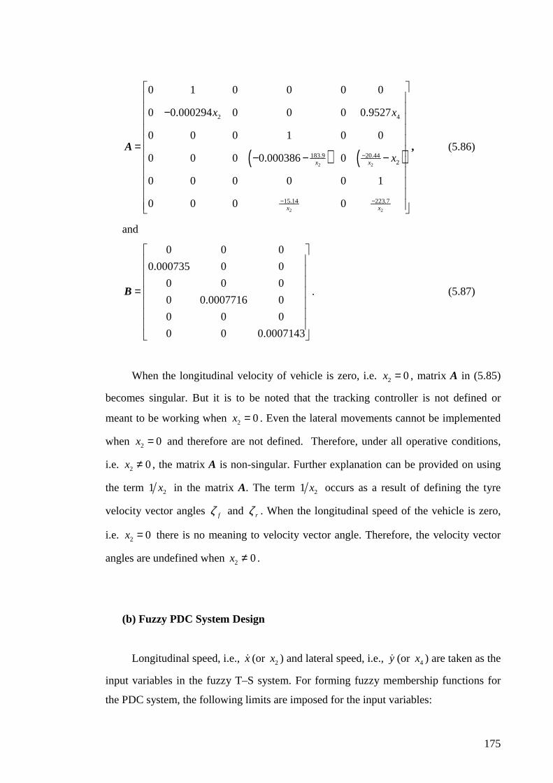
175
( ) ( )2 2
2 2
2 4
183.9 20.442
15.14 223.7
0 1 0 0 0 0
0 0.000294 0 0 0 0.9527
0 0 0 1 0 0
0 0 0 0.000386 0
0 0 0 0 0 1
0 0 0 0
x x
x x
x x
x−
− −
− = − − −
A , (5.86)
and
0 0 0
0.000735 0 0
0 0 0
0 0.0007716 0
0 0 0
0 0 0.0007143
=
B . (5.87)
When the longitudinal velocity of vehicle is zero, i.e. 2 0x = , matrix A in (5.85)
becomes singular. But it is to be noted that the tracking controller is not defined or
meant to be working when 2 0x = . Even the lateral movements cannot be implemented
when 2 0x = and therefore are not defined. Therefore, under all operative conditions,
i.e. 2 0x ≠ , the matrix A is non-singular. Further explanation can be provided on using
the term 21 x in the matrix A. The term 21 x occurs as a result of defining the tyre
velocity vector angles fζ and rζ . When the longitudinal speed of the vehicle is zero,
i.e. 2 0x = there is no meaning to velocity vector angle. Therefore, the velocity vector
angles are undefined when 2 0x ≠ .
(b) Fuzzy PDC System Design
Longitudinal speed, i.e., xɺ (or 2x ) and lateral speed, i.e., yɺ (or 4x ) are taken as the
input variables in the fuzzy T–S system. For forming fuzzy membership functions for
the PDC system, the following limits are imposed for the input variables:
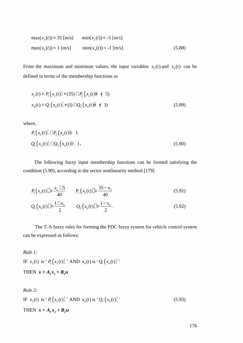
176
2max( ( ))x t = 35 [m/s] 2min( ( ))x t = -5 [m/s]
4max( ( ))x t = 1 [m/s] 4min( ( ))x t = -1 [m/s]. (5.88)
From the maximum and minimum values, the input variables 2( )x t and 4( )x t can be
defined in terms of the membership functions as
( ) ( )2 1 2 2 2( ) ( ) (35) ( ) ( 5)x t P x t P x t= × + × −
( ) ( )4 1 4 2 4( ) ( ) (1) ( ) ( 1)x t Q x t Q x t= × + × − (5.89)
where,
( ) ( )1 2 2 2( ) ( ) 1P x t P x t+ =
( ) ( )1 4 2 4( ) ( ) 1Q x t Q x t+ = . (5.90)
The following fuzzy input membership functions can be formed satisfying the
condition (5.90), according to the sector nonlinearity method [179]
( ) 21 2
5( )
40
xP x t
+= ( ) 22 2
35( )
40
xP x t
−= (5.91)
( ) 41 4
1( )
2
xQ x t
+= ( ) 42 4
1( ) .
2
xQ x t
−= (5.92)
The T–S fuzzy rules for forming the PDC fuzzy system for vehicle control system
can be expressed as follows:
Rule 1:
IF 2( )x t is ‘ ( )1 2( )P x t ’ AND 4( )x t is ‘ ( )1 4( )Q x t ’
THEN =ɺ 1 1 1x A x + B u
Rule 2:
IF 2( )x t is ‘ ( )1 2( )P x t ’ AND 4( )x t is ‘ ( )2 4( )Q x t ’ (5.93)
THEN ɺ 2 2 2x = A x + B u

177
Rule 3:
IF 2( )x t is ‘ ( )2 2( )P x t ’ AND 4( )x t is ‘ ( )1 4( )Q x t ’
THEN ɺ 3 3 3x = A x + B u
Rule 4:
IF 2( )x t is ‘ ( )2 2( )P x t ’ AND 4( )x t is ‘ ( )2 4( )Q x t ’
THEN ɺ 4 4 4x = A x + B u
(c) Design of Local Models for Simplified Vehicle Model
In order to obtain solutions for 1A , 2A , 3A and 4A matrices, the following linear
matrix equation is formed according to the fuzzy PDC principle and then solved, i.e.,
( ) ( ) ( ) ( ) ( ) ( )( ) ( )
1 2 1 4 1 1 2 2 4 2 2 2 1 4 3
2 2 2 4 4
( ) ( ) ( ) ( ) ( ) ( )
( ) ( ) .
P x t Q x t P x t Q x t P x t Q x t
P x t Q x t
= × × + × × + × ×
+ × ×
A A A A
A
(5.94)
The PDC equivalent system matrices for vehicle models are obtained as follows
(with substitution of known values as provided in (5.88) in the linear matrix equation
(5.94)):
( ) ( )2 2
2 2
1183.9 20.44
15.14 223.7
0 1 0 0 0 0
0 0.0103 0 0 0 0.9527
0 0 0 1 0 0
0 0 0 0.000386 0 35
0 0 0 0 0 1
0 0 0 0
x x
x x
−
− −
− = − − −
A (5.95)

178
( ) ( )2 2
2 2
2183.9 20.44
15.14 223.7
0 1 0 0 0 0
0 0.0103 0 0 0 0.9527
0 0 0 1 0 0
0 0 0 0.000386 0 35
0 0 0 0 0 1
0 0 0 0
x x
x x
−
− −
− − = − − −
A (5.96)
( ) ( )2 2
2 2
3183.9 20.44
15.14 223.7
0 1 0 0 0 0
0 0.00147 0 0 0 0.9527
0 0 0 1 0 0
0 0 0 0.000386 0 5
0 0 0 0 0 1
0 0 0 0
x x
x x
−
− −
= − − +
A (5.97)
( ) ( )2 2
2 2
4183.9 20.44
15.14 223.7
0 1 0 0 0 0
0 0.00147 0 0 0 0.9527
0 0 0 1 0 0
0 0 0 0.000386 0 5
0 0 0 0 0 1
0 0 0 0
x x
x x
−
− −
− = − − +
A . (5.98)
To obtain 1B , 2B , 3B and 4B matrices, it is taken as
0 0 0
0.000735 0 0
0 0 0
0 0.0007716 0
0 0 0
0 0 0.0007143
=
1 2 3 4B = B = B = B . (5.99)

179
The defuzzification in the PDC system is carried out as follows, and obtained the
system output as
4
1
( ( ))i i ii
x tη=
= +∑ɺɺx A x B u (5.100)
where
( ) ( )1 1 2 1 4( ( )) ( ) ( )x t P x t Q x tη = ×
( ) ( )1 1 2 2 4( ( )) ( ) ( )x t P x t Q x tη = × (5.101)
( ) ( )1 2 2 1 4( ( )) ( ) ( )x t P x t Q x tη = ×
( ) ( )1 2 2 2 4( ( )) ( ) ( )x t P x t Q x tη = × .
According to the design method, i.e., sector nonlinearity method, this T–S fuzzy
system exactly represents the vehicle model provided in (5.81) in the region [-5, 35]× [-
1, 1] of 2x – 4x space [179].
The fuzzy input membership functions of the developed PDC based T–S system
are provided below in Fig. 5.55.
Fig. 5.55 Fuzzy input membership functions
(ii) Synthesis of Local Adaptive Fuzzy Controllers for PDC System
The subtractive clustering method was used to obtain the basic fuzzy systems for
the adaptive fuzzy controllers similar to the procedure explained in Chapter 4. The final
fuzzy membership function centres and standard deviations (Gaussian) were then
obtained using the ANFIS method with further tuning.
(a) Input 2( )x t (b) Input 4( )x t
-5 35 20 -1 1 0
( )1 2( )P x t ( )2 2( )P x t ( )1 4( )Q x t ( )2 4( )Q x t
1 1

180
(a) T –S Fuzzy Rules for Longitudinal and Lateral Vehicle Controllers in the PDC System
The fuzzy PDC rules that contain the adaptive fuzzy controllers are described as
follows:
Rule 1:
IF 2( )x t is ‘ ( )1 2( )P x t ’ AND 4( )x t is ‘ ( )1 4( )Q x t ’
THEN ( )
( )11
11
ˆ ( )
ˆ ( )
T1x p dx px sx xx
T1y dy py sy yy
u = x k e k e u h q
u = k e k e u h q
+ + + + −
+ + + −
ɺɺ ɺ ɺ
ɺ ɺ
ψ θ
ψ θ
Rule 2:
IF 2( )x t is ‘ ( )1 2( )P x t ’ AND 4( )x t is ‘ ( )2 4( )Q x t ’
THEN ( )
( )2 22
2 22
ˆ ( )
ˆ ( )
Tx p dx px sx xx
Ty dy py sy yy
u = x k e k e u h q
u = k e k e u h q
+ + + + −
+ + + −
ɺɺ ɺ ɺ
ɺ ɺ
ψ θ
ψ θ
Rule 3: (5.102)
IF 2( )x t is ‘ ( )2 2( )P x t ’ AND 4( )x t is ‘ ( )1 4( )Q x t ’
THEN ( )
( )3 33
3 33
ˆ ( )
ˆ ( )
Tx p dx px sx xx
Ty dy py sy yy
u = x k e k e u h q
u = k e k e u h q
+ + + + −
+ + + −
ɺɺ ɺ ɺ
ɺ ɺ
ψ θ
ψ θ
Rule 4:
IF 2( )x t is ‘ ( )2 2( )P x t ’ AND 4( )x t is ‘ ( )2 4( )Q x t ’
THEN ( )
( )4 44
4 44
ˆ ( )
ˆ ( )
Tx p dx px sx xx
Ty dy py sy yy
u = x k e k e u h q
u = k e k e u h q
+ + + + −
+ + + −
ɺɺ ɺ ɺ
ɺ ɺ
ψ θ
ψ θ.
( )T
ixψ θ where 1, , 4i = … , are the control outputs from the adaptive fuzzy
longitudinal controllers, and ( )T
iyψ θ , where 1, , 4i = … , are the control outputs from
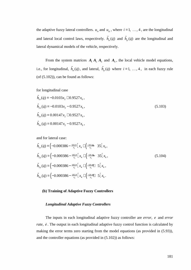
181
the adaptive fuzzy lateral controllers. ixu and iyu , where 1, , 4i = … , are the longitudinal
and lateral local control laws, respectively. ˆ ( )ixh qɺ and ˆ ( )iyh qɺ are the longitudinal and
lateral dynamical models of the vehicle, respectively.
From the system matrices 1A 2A 3A and 4A , the local vehicle model equations,
i.e., for longitudinal, ( )ixh qɺ , and lateral, ( )iyh qɺ where 1, , 4i = … , in each fuzzy rule
(of (5.102)), can be found as follows:
for longitudinal case
1 2 6ˆ ( ) 0.0103 0.9527xh q x x= − +ɺ ,
2 2 6ˆ ( ) 0.0103 0.9527xh q x x= − −ɺ , (5.103)
3 2 6ˆ ( ) 0.00147 0.9527xh q x x= +ɺ ,
4 2 6ˆ ( ) 0.00147 0.9527xh q x x= −ɺ ,
and for lateral case:
( ) ( )2 2
183.9 20.441 4 6ˆ ( ) 0.000386 35y x xh q x x−= − − + −ɺ ,
( ) ( )2 2
183.9 20.442 4 6
ˆ ( ) 0.000386 35y x xh q x x−= − − + −ɺ , (5.104)
( ) ( )2 2
183.9 20.443 4 6ˆ ( ) 0.000386 5y x xh q x x−= − − + +ɺ ,
( ) ( )2 2
183.9 20.444 4 6
ˆ ( ) 0.000386 5y x xh q x x−= − − + +ɺ .
(b) Training of Adaptive Fuzzy Controllers
Longitudinal Adaptive Fuzzy Controllers
The inputs in each longitudinal adaptive fuzzy controller are error, e and error
rate, eɺ . The output in each longitudinal adaptive fuzzy control function is calculated by
making the error terms zero starting from the model equations (as provided in (5.93)),
and the controller equations (as provided in (5.102)) as follows:
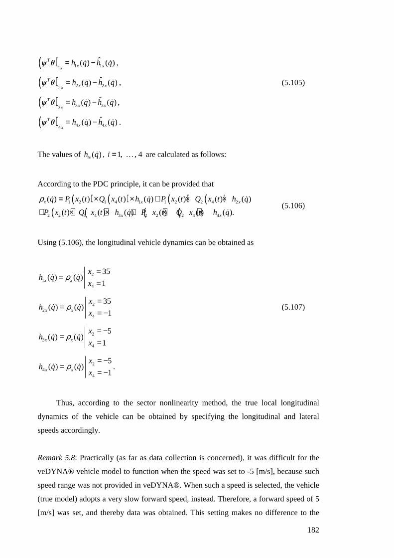
182
( ) 1 11
ˆ( ) ( )Tx xx
h q h q= −ɺ ɺψ θ ,
( ) 2 22
ˆ( ) ( )Tx xx
h q h q= −ɺ ɺψ θ , (5.105)
( ) 3 33
ˆ( ) ( )Tx xx
h q h q= −ɺ ɺψ θ ,
( ) 4 44
ˆ( ) ( )Tx xx
h q h q= −ɺ ɺψ θ .
The values of ( )ixh qɺ , 1, , 4i = … are calculated as follows:
According to the PDC principle, it can be provided that
( ) ( ) ( ) ( )( ) ( ) ( ) ( )
1 2 1 4 1 1 2 2 4 2
2 2 1 4 3 2 2 2 4 4
( ) ( ) ( ) ( ) ( ) ( ) ( )
( ) ( ) ( ) ( ) ( ) ( ).
x x x
x x
q P x t Q x t h q P x t Q x t h q
P x t Q x t h q P x t Q x t h q
ρ = × × + × ×
+ × × + × ×
ɺ ɺ ɺ
ɺ ɺ (5.106)
Using (5.106), the longitudinal vehicle dynamics can be obtained as
21
4
35( ) ( )
1x x
xh q q
xρ
==
=ɺ ɺ
22
4
35( ) ( )
1x x
xh q q
xρ
==
= −ɺ ɺ (5.107)
23
4
5( ) ( )
1x x
xh q q
xρ
= −=
=ɺ ɺ
24
4
5( ) ( )
1x x
xh q q
xρ
= −=
= −ɺ ɺ .
Thus, according to the sector nonlinearity method, the true local longitudinal
dynamics of the vehicle can be obtained by specifying the longitudinal and lateral
speeds accordingly.
Remark 5.8: Practically (as far as data collection is concerned), it was difficult for the
veDYNA® vehicle model to function when the speed was set to -5 [m/s], because such
speed range was not provided in veDYNA®. When such a speed is selected, the vehicle
(true model) adopts a very slow forward speed, instead. Therefore, a forward speed of 5
[m/s] was set, and thereby data was obtained. This setting makes no difference to the
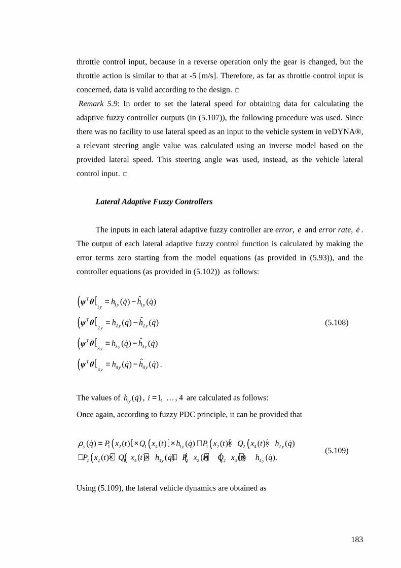
183
throttle control input, because in a reverse operation only the gear is changed, but the
throttle action is similar to that at -5 [m/s]. Therefore, as far as throttle control input is
concerned, data is valid according to the design.
Remark 5.9: In order to set the lateral speed for obtaining data for calculating the
adaptive fuzzy controller outputs (in (5.107)), the following procedure was used. Since
there was no facility to use lateral speed as an input to the vehicle system in veDYNA®,
a relevant steering angle value was calculated using an inverse model based on the
provided lateral speed. This steering angle was used, instead, as the vehicle lateral
control input.
Lateral Adaptive Fuzzy Controllers
The inputs in each lateral adaptive fuzzy controller are error, e and error rate, eɺ .
The output of each lateral adaptive fuzzy control function is calculated by making the
error terms zero starting from the model equations (as provided in (5.93)), and the
controller equations (as provided in (5.102)) as follows:
( ) 1 11
ˆ( ) ( )Ty yy
h q h q= −ɺ ɺψ θ
( ) 2 22
ˆ( ) ( )Ty yy
h q h q= −ɺ ɺψ θ (5.108)
( ) 3 33
ˆ( ) ( )Ty yy
h q h q= −ɺ ɺψ θ
( ) 4 44
ˆ( ) ( )Ty yy
h q h q= −ɺ ɺψ θ .
The values of ( )iyh qɺ , 1, , 4i = … are calculated as follows:
Once again, according to fuzzy PDC principle, it can be provided that
( ) ( ) ( ) ( )( ) ( ) ( ) ( )
1 2 1 4 1 1 2 2 4 2
2 2 1 4 3 2 2 2 4 4
( ) ( ) ( ) ( ) ( ) ( ) ( )
( ) ( ) ( ) ( ) ( ) ( ).
y y y
y y
q P x t Q x t h q P x t Q x t h q
P x t Q x t h q P x t Q x t h q
ρ = × × + × ×
+ × × + × ×
ɺ ɺ ɺ
ɺ ɺ (5.109)
Using (5.109), the lateral vehicle dynamics are obtained as
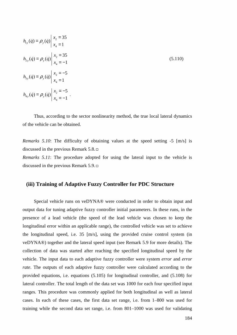
184
21
4
35( ) ( )
1y y
xh q q
xρ
==
=ɺ ɺ
22
4
35( ) ( )
1y y
xh q q
xρ
==
= −ɺ ɺ (5.110)
23
4
5( ) ( )
1y y
xh q q
xρ
= −=
=ɺ ɺ
24
4
5( ) ( )
1y y
xh q q
xρ
= −=
= −ɺ ɺ .
Thus, according to the sector nonlinearity method, the true local lateral dynamics
of the vehicle can be obtained.
Remarks 5.10: The difficulty of obtaining values at the speed setting -5 [m/s] is
discussed in the previous Remark 5.8.
Remarks 5.11: The procedure adopted for using the lateral input to the vehicle is
discussed in the previous Remark 5.9.
(iii) Training of Adaptive Fuzzy Controller for PDC Structure
Special vehicle runs on veDYNA® were conducted in order to obtain input and
output data for tuning adaptive fuzzy controller initial parameters. In these runs, in the
presence of a lead vehicle (the speed of the lead vehicle was chosen to keep the
longitudinal error within an applicable range), the controlled vehicle was set to achieve
the longitudinal speed, i.e. 35 [m/s], using the provided cruise control system (in
veDYNA®) together and the lateral speed input (see Remark 5.9 for more details). The
collection of data was started after reaching the specified longitudinal speed by the
vehicle. The input data to each adaptive fuzzy controller were system error and error
rate. The outputs of each adaptive fuzzy controller were calculated according to the
provided equations, i.e. equations (5.105) for longitudinal controller, and (5.108) for
lateral controller. The total length of the data set was 1000 for each four specified input
ranges. This procedure was commonly applied for both longitudinal as well as lateral
cases. In each of these cases, the first data set range, i.e. from 1–800 was used for
training while the second data set range, i.e. from 801–1000 was used for validating
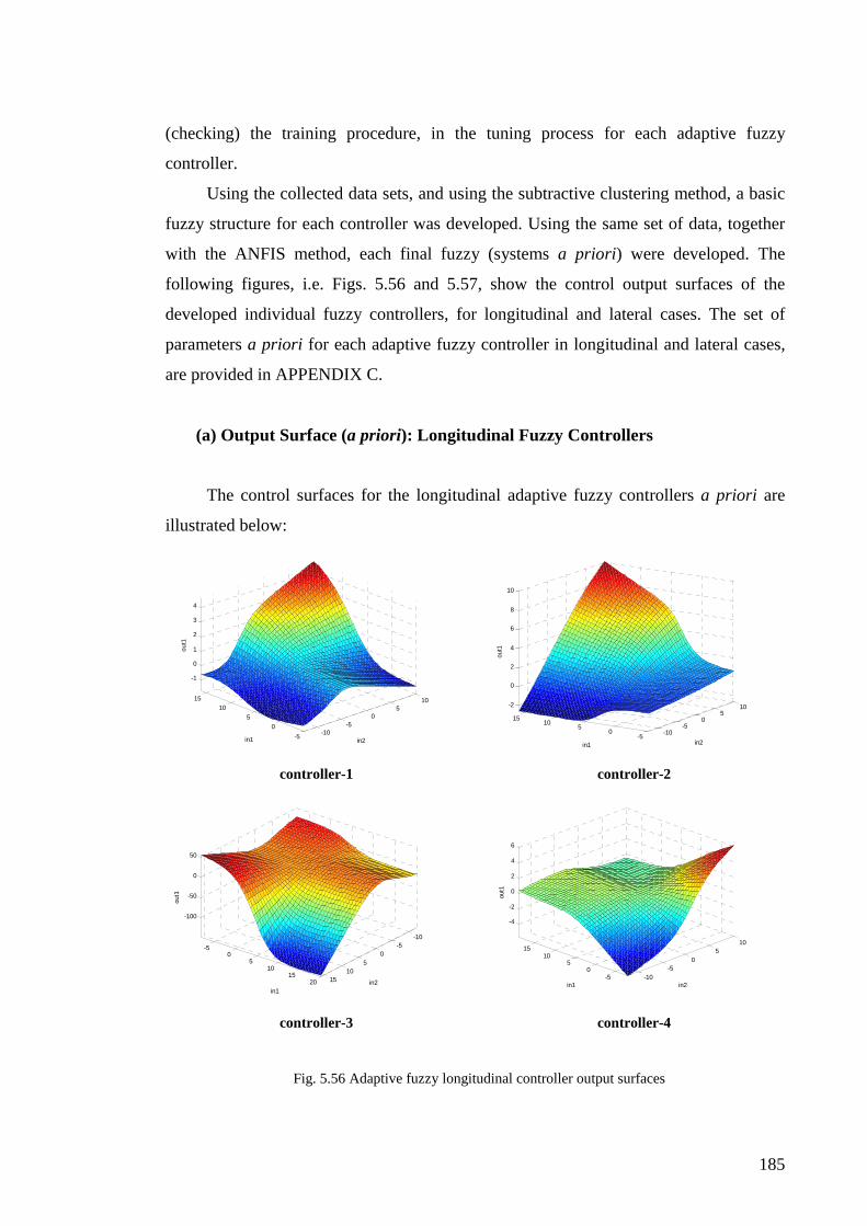
185
(checking) the training procedure, in the tuning process for each adaptive fuzzy
controller.
Using the collected data sets, and using the subtractive clustering method, a basic
fuzzy structure for each controller was developed. Using the same set of data, together
with the ANFIS method, each final fuzzy (systems a priori) were developed. The
following figures, i.e. Figs. 5.56 and 5.57, show the control output surfaces of the
developed individual fuzzy controllers, for longitudinal and lateral cases. The set of
parameters a priori for each adaptive fuzzy controller in longitudinal and lateral cases,
are provided in APPENDIX C.
(a) Output Surface (a priori): Longitudinal Fuzzy Controllers
The control surfaces for the longitudinal adaptive fuzzy controllers a priori are
illustrated below:
-10-5
05
10
-5
0
5
10
15
-1
0
1
2
3
4
in2in1
out1
-10
-50
510
-50
510
15
-2
0
2
4
6
8
10
in2in1
out1
controller-1 controller-2
-10-5
05
1015
-50
510
1520
-100
-50
0
50
in2in1
out1
-10
-50
510
-50
510
15
-4
-2
0
2
4
6
in2in1
out1
controller-3
controller-4
Fig. 5.56 Adaptive fuzzy longitudinal controller output surfaces
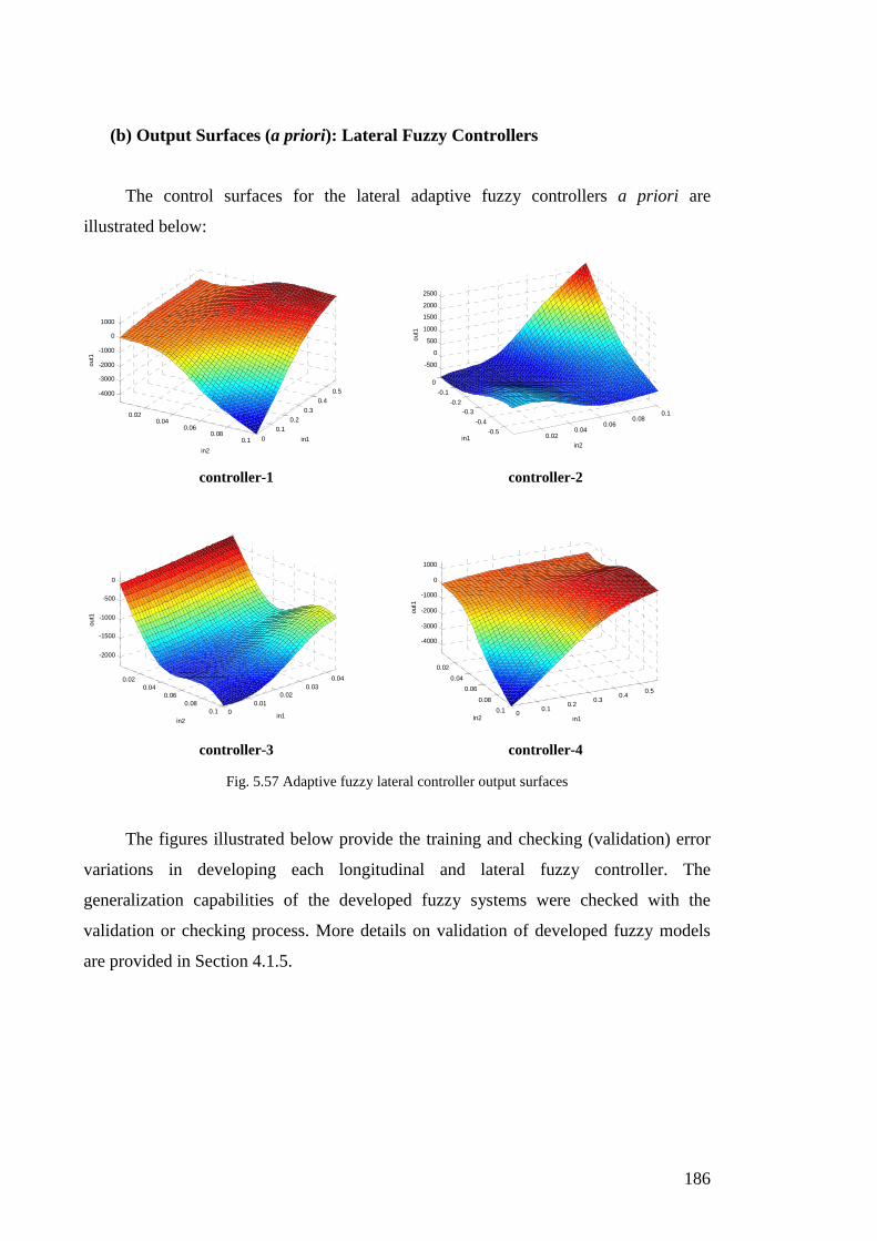
186
(b) Output Surfaces (a priori): Lateral Fuzzy Controllers
The control surfaces for the lateral adaptive fuzzy controllers a priori are
illustrated below:
0.020.04
0.060.08
0.1 0
0.1
0.2
0.3
0.4
0.5-4000
-3000
-2000
-1000
0
1000
in1
in2
out1
0.02
0.040.06
0.080.1
-0.5
-0.4
-0.3
-0.2
-0.1
0
-500
0
500
1000
1500
2000
2500
in2in1
out1
controller-1 controller-2
0.020.04
0.060.08
0.1 00.01
0.020.03
0.04
-2000
-1500
-1000
-500
0
in1in2
out1
0.02
0.04
0.06
0.08
0.1 00.1
0.20.3
0.40.5
-4000
-3000
-2000
-1000
0
1000
in1in2
out1
controller-3 controller-4
Fig. 5.57 Adaptive fuzzy lateral controller output surfaces
The figures illustrated below provide the training and checking (validation) error
variations in developing each longitudinal and lateral fuzzy controller. The
generalization capabilities of the developed fuzzy systems were checked with the
validation or checking process. More details on validation of developed fuzzy models
are provided in Section 4.1.5.
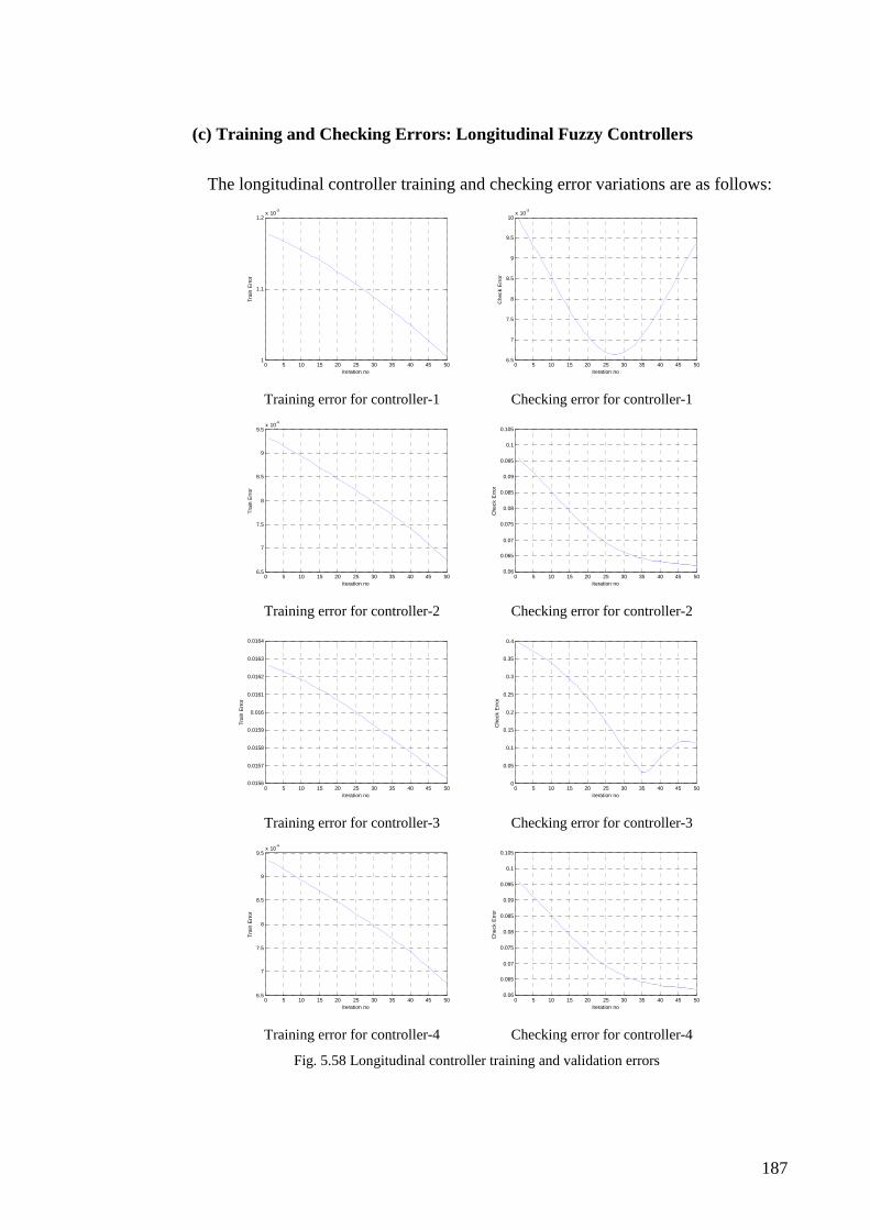
187
(c) Training and Checking Errors: Longitudinal Fuzzy Controllers
The longitudinal controller training and checking error variations are as follows:
0 5 10 15 20 25 30 35 40 45 501
1.1
1.2x 10
-3
iteration no
Tra
in E
rror
0 5 10 15 20 25 30 35 40 45 50
6.5
7
7.5
8
8.5
9
9.5
10x 10
-3
iteration no
Che
ck E
rror
Training error for controller-1 Checking error for controller-1
0 5 10 15 20 25 30 35 40 45 506.5
7
7.5
8
8.5
9
9.5x 10
-4
iteration no
Tra
in E
rror
0 5 10 15 20 25 30 35 40 45 50
0.06
0.065
0.07
0.075
0.08
0.085
0.09
0.095
0.1
0.105
iteration no
Che
ck E
rror
Training error for controller-2 Checking error for controller-2
0 5 10 15 20 25 30 35 40 45 500.0156
0.0157
0.0158
0.0159
0.016
0.0161
0.0162
0.0163
0.0164
iteration no
Tra
in E
rror
0 5 10 15 20 25 30 35 40 45 50
0
0.05
0.1
0.15
0.2
0.25
0.3
0.35
0.4
iteration no
Che
ck E
rror
Training error for controller-3 Checking error for controller-3
0 5 10 15 20 25 30 35 40 45 506.5
7
7.5
8
8.5
9
9.5x 10
-4
iteration no
Tra
in E
rror
0 5 10 15 20 25 30 35 40 45 50
0.06
0.065
0.07
0.075
0.08
0.085
0.09
0.095
0.1
0.105
iteration no
Che
ck E
rror
Training error for controller-4 Checking error for controller-4
Fig. 5.58 Longitudinal controller training and validation errors
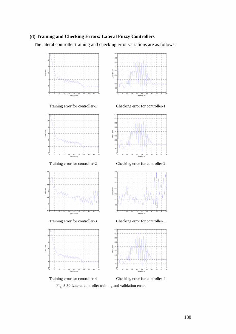
188
(d) Training and Checking Errors: Lateral Fuzzy Controllers
The lateral controller training and checking error variations are as follows:
0 5 10 15 20 25 30 35 40 45 505
6
7
8
9
10
11
iteration no
Tra
in E
rror
0 5 10 15 20 25 30 35 40 45 50
0
50
100
150
200
250
300
350
400
450
iteration no
Che
ck E
rror
Training error for controller-1 Checking error for controller-1
0 5 10 15 20 25 30 35 40 45 505
6
7
8
9
10
11
iteration no
Tra
in E
rror
0 5 10 15 20 25 30 35 40 45 50
0
50
100
150
200
250
300
350
400
450
iteration no
Che
ck E
rror
Training error for controller-2 Checking error for controller-2
0 5 10 15 20 25 30 35 40 45 504.5
5
5.5
6
6.5
7
7.5
iteration no
Tra
in E
rror
0 5 10 15 20 25 30 35 40 45 50
0
50
100
150
200
250
300
350
iteration no
Che
ck E
rror
Training error for controller-3 Checking error for controller-3
0 5 10 15 20 25 30 35 40 45 505
6
7
8
9
10
11
iteration no
Tra
in E
rror
0 5 10 15 20 25 30 35 40 45 50
0
50
100
150
200
250
300
350
400
450
iteration no
Che
ck E
rror
Training error for controller-4 Checking error for controller-4
Fig. 5.59 Lateral controller training and validation errors

189
5.2.5 Simulation Studies, Results and Discussion
(i) Simulation Setup
The simulation setup for this section was similar to the one provided in Chapter 4
for the single-adaptive fuzzy controller system, except for facts otherwise stated in this
section. The simulation setup included the veDYNA® setup, simulation profile details
and other settings.
The gains in adaptive fuzzy controllers were taken as, 1 2 3 4 0.03x x x xγ γ γ γ= = = =
for longitudinal case, and 1 2 3 4 0.01y y y yγ γ γ γ= = = = for lateral case, in the PDC based
multiple-model adaptive fuzzy controller setup.
(ii) Simulation Results and Discussion
In the following figures depicting simulation results, each performance parameter
of the multiple-model fuzzy PDC-based adaptive fuzzy controller (solid blue line) is
compared against that of the single-adaptive fuzzy controller (dotted red line).
(a) Normal Cruising Conditions: Multiple-Model PDC-based Adaptive Fuzzy Control
The following simulation results provide the performance of the developed PDC-
based multiple-model adaptive fuzzy controller against the results of the single-adaptive
fuzzy controller under normal cruising conditions without the presence of any external
disturbances.
In the variations of tracking performances in the lateral and longitudinal cases,
PDC-based multiple-model controller has shown some improved display, as provided in
Figs. 5.60–5.61, over the single-adaptive fuzzy controller. There is a clear indication of
elimination of transient effects together with high amplitudes by the PDC fuzzy
controller.

190
0 10 20 30 40 50 60-2
0
2
4
6
8
10
12
14
actual simulation time [s]
Long
itudi
nal E
rror
[m
]
longitudinal error with PDC multi-adaptive fuzzy
longitudinal error with single-adaptive fuzzy
Fig. 5.60 Longitudinal error: PDC-based multiple-adaptive fuzzy with blending (RMS: 3.064) vs. single-adaptive fuzzy (RMS: 3.158)
0 10 20 30 40 50 60-0.01
-0.005
0
0.005
0.01
0.015
0.02
actual simulation time [s]
Late
ral E
rror
[m
]
lateral error with PDC multiple-adaptive fuzzy with blending [m]
lateral error with single-adaptive fuzzy [m]
Fig. 5.61 Lateral error: PDC-based multiple-adaptive fuzzy with blending (RMS: 0.001119) vs. single-adaptive fuzzy (RMS: 0.003837)
When it comes to variation of pitch angle, the two controllers fared similarly
except for a high ‘spike’ by the PDC multiple-model fuzzy controller towards the point
5 [s] on the time-scale. This is shown in Fig. 5.62 below. But, this cannot be considered
as overly excessive.
0 10 20 30 40 50 60-0.05
-0.04
-0.03
-0.02
-0.01
0
0.01
0.02
0.03
0.04
actual simulation time [s]
Pitc
h A
ngle
[ra
d]
pitch angle with PDC multi-adaptive fuzzy[rad]
pitch angle with single-adaptive fuzzy[rad]
Fig. 5.62 Pitch angle: PDC-based multiple-adaptive fuzzy with blending (RMS: 0.01225) vs. single-adaptive fuzzy (RMS: 0.01195)

191
0 10 20 30 40 50 60-0.025
-0.02
-0.015
-0.01
-0.005
0
0.005
0.01
0.015
0.02
0.025
actual simulation time [s]
Rol
l Ang
le [
rad]
roll angle with single-adaptive fuzzy [rad]
roll angle with PDC multi-adaptive fuzzy [rad]
Fig. 5.63 Roll angle: PDC-based multiple-adaptive fuzzy with blending (RMS: 0.01083) vs. single-adaptive fuzzy (RMS: 0.01086)
0 10 20 30 40 50 60-0.1
-0.05
0
0.05
0.1
0.15
actual simulation time [s]
Rol
l Rat
e [r
ad/s
]
roll rate with PDC multi-adaptive fuzzy [rad/s]
roll rate with single-adaptive fuzzy [rad/s]
Fig. 5.64 Roll rate: PDC-based multiple-adaptive fuzzy with blending (RMS: 0.008043) vs. single-adaptive fuzzy (RMS: 0.01)
0 10 20 30 40 50 60-0.015
-0.01
-0.005
0
0.005
0.01
0.015
0.02
actual simulation time [s]
Sid
e S
lip A
ngle
[ra
d]
side slip angle with single-adaptive fuzzy
side slip angle with PDC multi-adaptive fuzzy
Fig. 5.65 Side-slip angle: PDC-based multiple-adaptive fuzzy with blending (RMS: 0.007201) vs. single-adaptive fuzzy (RMS: 0.007206)
Roll angle variations, as shown in Fig. 5.63, for the two controllers have been
similar to each other. But, the PDC multiple-adaptive fuzzy controller has shown some
chattering effects slightly, e.g. 42 – 43 [s]. When the variation of roll rate, as provided
in Fig. 5.64 is considered, the PDC multiple-adaptive fuzzy controller has shown some
significant improvements in comparison to its counterpart during high-values, e.g. 37 –
43 [s]. But during periods with lower values of roll-rate, the single-adaptive fuzzy
controller has outperformed its counterpart, slightly, e.g. throughout 22 –37 [s], 47 –60

192
[s]. As illustrated in Fig. 5.65, the PDC multiple-adaptive fuzzy control has mildly
improved the response of side-slip angle especially with transients as against its
counterpart. It can be said that lateral stability ensured by the PDC multiple-model
adaptive fuzzy controller stands at a similar level to that by the single-adaptive fuzzy
controller, as evidenced by similar variations of roll angle, roll rate and side-slip angle.
As shown in Fig. 5.66, the variations of lateral acceleration do not go beyond 4
[m/s2], therefore, the PDC based multiple-model adaptive fuzzy controller has managed
to contain lateral acceleration within low limits as far as the design requirements of
passenger vehicles are concerned [178].
0 10 20 30 40 50 60-4
-3
-2
-1
0
1
2
3
actual simulation time [s]
Late
ral A
ccel
erat
ion
[m/s
2 ]
lateral acceleration with PDC multi-adaptive fuzzy [m/s 2]
lateral acceleration with single-adaptive fuzzy [m/s 2]
Fig. 5.66 Lateral acceleration: PDC-based multiple-adaptive fuzzy with blending (RMS: 1.265) vs. single-adaptive fuzzy (RMS: 1.264)
Overall, in the presence of normal cruising conditions, the performance of the
PDC-based multiple-adaptive fuzzy controller has been significantly improved with
regard to lateral and longitudinal tracking in comparison to that of the single-adaptive-
fuzzy controller. While these tracking performance levels are maintained, the PDC
based multiple-model controller has ensured an acceptable level of lateral stability in
comparison to the single-adaptive fuzzy controller. Lateral acceleration has also been
maintained throughout at an acceptable standard level by both controllers.
(b) External Disturbances: Multiple-Model PDC-based Adaptive Fuzzy Control
In the following set of simulations, the developed PDC-based multiple-model
adaptive fuzzy controller was tested against the single-adaptive fuzzy controller under a
number of external disturbances. These disturbances included addition of an un-
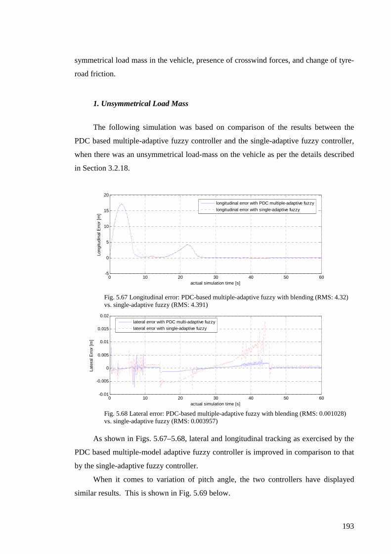
193
symmetrical load mass in the vehicle, presence of crosswind forces, and change of tyre-
road friction.
1. Unsymmetrical Load Mass
The following simulation was based on comparison of the results between the
PDC based multiple-adaptive fuzzy controller and the single-adaptive fuzzy controller,
when there was an unsymmetrical load-mass on the vehicle as per the details described
in Section 3.2.18.
0 10 20 30 40 50 60-5
0
5
10
15
20
actual simulation time [s]
Long
itudi
nal E
rror
[m
]
longitudinal error with PDC multiple-adaptive fuzzy
longitudinal error with single-adaptive fuzzy
Fig. 5.67 Longitudinal error: PDC-based multiple-adaptive fuzzy with blending (RMS: 4.32) vs. single-adaptive fuzzy (RMS: 4.391)
0 10 20 30 40 50 60-0.01
-0.005
0
0.005
0.01
0.015
0.02
actual simulation time [s]
Late
ral E
rror
[m
]
lateral error with PDC multi-adaptive fuzzy
lateral error with single-adaptive fuzzy
Fig. 5.68 Lateral error: PDC-based multiple-adaptive fuzzy with blending (RMS: 0.001028) vs. single-adaptive fuzzy (RMS: 0.003957)
As shown in Figs. 5.67–5.68, lateral and longitudinal tracking as exercised by the
PDC based multiple-model adaptive fuzzy controller is improved in comparison to that
by the single-adaptive fuzzy controller.
When it comes to variation of pitch angle, the two controllers have displayed
similar results. This is shown in Fig. 5.69 below.

194
0 10 20 30 40 50 60-0.05
-0.04
-0.03
-0.02
-0.01
0
0.01
0.02
actual simulation time [s]
Pitc
h A
ngle
[ra
d]
pitch angle with PDC multi-adaptive fuzzy [rad]
pitch angle with single-adaptive fuzzy [rad]
Fig. 5.69 Pitch angle: PDC-based multiple-adaptive fuzzy with blending (RMS: 0.02009) vs. single-adaptive fuzzy (RMS: 0.01998)
0 10 20 30 40 50 60-0.04
-0.035
-0.03
-0.025
-0.02
-0.015
-0.01
-0.005
0
0.005
0.01
actual simulation time [s]
Rol
l Ang
le [
rad]
roll angle with single-adaptive fuzzy[rad]
roll angle with PDC multi-adaptive fuzzy[rad]
Fig. 5.70 Roll angle: PDC-based multiple-adaptive fuzzy with blending (RMS: 0.01767) vs. single-adaptive fuzzy (RMS: 0.01766)
0 10 20 30 40 50 60-0.2
-0.15
-0.1
-0.05
0
0.05
0.1
0.15
actual simulation time [s]
Rol
l Rat
e [r
ad/s
]
roll rate with PDC multi-adaptive fuzzy[rad/s]
roll rate with single-adaptive fuzzy[rad/s]
Fig. 5.71 Roll rate: PDC-based multiple-adaptive fuzzy with blending (RMS: 0.01443) vs. single-adaptive fuzzy (RMS: 0.015)

195
0 10 20 30 40 50 60-0.04
-0.03
-0.02
-0.01
0
0.01
0.02
actual simulation time [s]
Sid
e S
lip A
ngle
[ra
d]
side slip angle with PDC multi-adaptive fuzzy[rad]
side slip angle with single-adaptive fuzzy[rad]
Fig. 5.72 Side-slip angle: PDC-based multiple-adaptive fuzzy with blending (RMS: 0.008227) vs. single-adaptive fuzzy (RMS: 0.008237)
The PDC multiple-adaptive fuzzy controller has shown the results of variations of
roll angle, roll rate and side-slip ratio as quite consistent in comparison to that of the
single-adaptive fuzzy controller, as shown in Figs. 5.70–5.72. Therefore, it can be said
that the PDC multiple-adaptive fuzzy controller has shown acceptable lateral stability
results in comparison to its counterpart.
As shown in Fig. 5.73, variations of lateral acceleration with regard to the PDC
based multiple-model adaptive fuzzy controller, have not gone beyond 4 [m/s2].
Therefore, the PDC based multiple-adaptive fuzzy controller has managed to contain
lateral acceleration within low limits as far as the design requirements of vehicles are
concerned [178].
0 10 20 30 40 50 60-4
-3
-2
-1
0
1
2
3
actual simulation time [s]
Late
ral A
ccel
erat
ion
[m/s
2 ]
lateral acceleration with PDC multiple-adaptive fuzzy with blending [m/s 2]
lateral acceleration with single-adaptive fuzzy [m/s 2]
Fig. 5.73 Lateral acceleration: PDC-based multiple-adaptive fuzzy with blending (RMS: 1.265) vs. single-adaptive fuzzy (RMS: 1.256)
Overall, in the presence of unsymmetrical load mass, the PDC based adaptive
fuzzy controller has managed to show significant improvements in lateral and
longitudinal tracking, in comparison to the single-adaptive fuzzy controller.

196
Performances of the former in lateral stability have also been consistent throughout.
Design requirements, too are satisfied where lateral acceleration variation is concerned.
2. Crosswind Effects
The following simulation results were obtained when there was a presence of a
continuous crosswind with a speed of 50 [m/s] through the global y-direction. More
details of this arrangement are described in Section 3.2.18.
Once again, the PDC based multiple-model adaptive fuzzy controller has shown
significant improvements over lateral and longitudinal tracking, as shown in Figs. 5.74–
5.75, in comparison to the single-adaptive fuzzy controller.
0 10 20 30 40 50 60-5
0
5
10
15
20
actual simulation time [s]
Long
itudi
nal E
rror
[m
]
longitudinal error with single-adaptive fuzzy
longitudinal error with PDC multi-adaptive fuzzy
Fig. 5.74 Longitudinal error: PDC-based multiple-adaptive fuzzy with blending (RMS: 3.12) vs. single-adaptive fuzzy (RMS: 3.742)
0 10 20 30 40 50 60-0.02
-0.01
0
0.01
0.02
0.03
0.04
actual simulation time [s]
Late
ral E
rror
[m
]
lateral error with PDC multiple-adaptive fuzzy with blending [m]
lateral error with single-adaptive fuzzy [m]
Fig. 5.75 Lateral error: PDC-based multiple-adaptive fuzzy with blending (RMS: 0.002672) vs. single-adaptive fuzzy (RMS: 0.005914)
Pitch angle, as shown in Fig. 5.76, of the PDC multiple-model control system
shows a variation that is similar to the variation shown by the single-adaptive fuzzy
controller.

197
As far as variations of roll angle, roll rate and side-slip angle go as shown in Figs.
5.77–5.79, the PDC multiple-adaptive fuzzy controller has shown some ‘spikes’. But
these ‘spikes’ will not make the variations excessively different from that of the single-
adaptive fuzzy controller. Therefore, the PDC multiple-adaptive fuzzy controller can be
said to maintain lateral stability at a level not much different from that of the single-
adaptive fuzzy controller.
0 10 20 30 40 50 60-0.04
-0.03
-0.02
-0.01
0
0.01
0.02
0.03
actual simulation time [s]
Pitc
h A
ngle
[ra
d]
pitch angle with single-adaptive fuzzy [rad]
pitch angle with PDC multi-adaptive fuzzy [rad]
Fig. 5.76 Pitch angle: PDC-based multiple-adaptive fuzzy with blending (RMS: 0.0117) vs. single-adaptive fuzzy (RMS: 0.01142)
0 10 20 30 40 50 60-0.06
-0.05
-0.04
-0.03
-0.02
-0.01
0
0.01
0.02
actual simulation time [s]
Rol
l Ang
le [
rad]
roll angle with PDC multiple-adaptive fuzzy with blending [rad]
roll angle with single-adaptive fuzzy [rad]
Fig. 5.77 Roll angle: PDC-based multiple-adaptive fuzzy with blending (RMS: 0.01419) vs. single-adaptive fuzzy (RMS: 0.01396)
0 10 20 30 40 50 60-0.5
-0.4
-0.3
-0.2
-0.1
0
0.1
0.2
0.3
0.4
actual simulation time [s]
Rol
l Rat
e [r
ad/s
]
roll rate with single-adaptive fuzzy [rad/s]
roll rate with PDC multi-adaptive fuzzy [rad/s]
Fig. 5.78 Roll rate: PDC-based multiple-adaptive fuzzy with blending (RMS: 0.03319) vs. single-adaptive fuzzy (RMS: 0.02222)

198
0 10 20 30 40 50 60-0.06
-0.04
-0.02
0
0.02
0.04
0.06
0.08
actual simulation time [s]
Sid
e-S
lip A
ngle
[ra
d]
side-slip angle with PDC multiple-adaptive fuzzy with blending [rad]
side-slip angle with single-adaptive fuzzy [rad]
Fig. 5.79 Side-slip angle: PDC-based multiple-adaptive fuzzy with blending (RMS: 0.01577) vs. single-adaptive fuzzy (RMS: 0.01438)
As far as lateral acceleration is concerned, the PDC multiple-model system tries to
keep the values within 4 [m/s2], thereby satisfying the design requirements of today’s
passenger vehicles [178].
0 10 20 30 40 50 60-4
-3
-2
-1
0
1
2
3
actual simulation time [s]
Late
ral A
ccel
erat
ion
[m/s
2 ]
lateral acceleration with PDC multiple-adaptive fuzzy with blending [m/s 2]
lateral acceleration with single-adaptive fuzzy [m/s 2]
Fig. 5.80 Lateral acceleration: PDC-based multiple-adaptive fuzzy with blending (RMS: 1.268) vs. single-adaptive fuzzy (RMS: 1.285)
Overall, in the presence of crosswind effects, the PDC multiple-model adaptive
fuzzy controller has shown some good performances of tracking in lateral and
longitudinal domains, once again exceeding the capacity of the single-adaptive fuzzy
system.
3. Tyre-Road Friction Change
The following simulation results show the performance of the PDC multiple-
adaptive fuzzy controller and the single-adaptive fuzzy controller when there was a
change of tyre-road friction in the range 100-200 [m], on the highway.

199
0 10 20 30 40 50 60-2
0
2
4
6
8
10
12
14
actual simulation time [s]
Long
itudi
nal E
rror
[m
]
longitudinal error with PDC multi-adaptive fuzzy
longitudinal error with single-adaptive fuzzy
Fig. 5.81 Longitudinal error: PDC-based multiple-adaptive fuzzy with blending (RMS: 3.065) vs. single-adaptive fuzzy (RMS: 3.158)
0 10 20 30 40 50 60-0.02
-0.015
-0.01
-0.005
0
0.005
0.01
0.015
actual simulation time [s]
Late
ral E
rror
[m
]
lateral error with PDC multiple-adaptive fuzzy with blending [m]
lateral error with single-adaptive fuzzy [m]
Fig. 5.82 Lateral error: PDC-based multiple-adaptive fuzzy with blending (RMS: 0.001217) vs. single-adaptive fuzzy (RMS: 0.003996)
0 10 20 30 40 50 60-0.05
-0.04
-0.03
-0.02
-0.01
0
0.01
0.02
0.03
0.04
actual simulation time [s]
Pitc
h A
ngle
[ra
d]
pitch angle with PDC multi-adaptive fuzzy
pitch angle with single-adaptive fuzzy
Fig. 5.83 Pitch angle: PDC-based multiple-adaptive fuzzy with blending (RMS: 0.0116) vs. single-adaptive fuzzy (RMS: 0.01144)
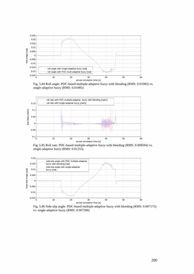
200
0 10 20 30 40 50 60-0.025
-0.02
-0.015
-0.01
-0.005
0
0.005
0.01
0.015
0.02
0.025
actual simulation time [s]
Rol
l Ang
le [
rad]
roll angle with single-adaptive fuzzy [rad]
roll angle with PDC multi-adaptive fuzzy [rad]
Fig. 5.84 Roll angle: PDC-based multiple-adaptive fuzzy with blending (RMS: 0.01085) vs. single-adaptive fuzzy (RMS: 0.01085)
0 10 20 30 40 50 60-0.1
-0.05
0
0.05
0.1
0.15
actual simulation time [s]
Rol
l Rat
e [r
ad/s
]
roll rate with PDC multiple-adaptive fuzzy with blending [rad/s]
roll rate with single-adaptive fuzzy [rad/s]
Fig. 5.85 Roll rate: PDC-based multiple-adaptive fuzzy with blending (RMS: 0.008594) vs. single-adaptive fuzzy (RMS: 0.01255)
0 10 20 30 40 50 60-0.015
-0.01
-0.005
0
0.005
0.01
0.015
0.02
actual simulation time [s]
Sid
e-S
lip A
ngle
[ra
d]
side-slip angle with PDC multiple-adaptive fuzzy with blending [rad]
side-slip angle with single-adaptive fuzzy [rad]
Fig. 5.86 Side-slip angle: PDC-based multiple-adaptive fuzzy with blending (RMS: 0.007175) vs. single-adaptive fuzzy (RMS: 0.007268)

201
0 10 20 30 40 50 60-4
-3
-2
-1
0
1
2
3
actual simulation time [s]
Late
ral A
ccel
erat
ion
[m/s
2 ]
lateral acceleratio with PDC multi-adaptive fuzzy [m/s 2]
lateral acceleratio with single-adaptive fuzzy [m/s 2]
Fig. 5.87 Lateral acceleration: PDC-based multiple-adaptive fuzzy with blending (RMS: 1.264) vs. single-adaptive fuzzy (RMS: 1.266)
Overall, in the presence of tyre-road friction changes, the PDC-based multiple-
adaptive fuzzy controller has demonstrated that it can perform better with longitudinal
and lateral tracking than the single-adaptive fuzzy controller (as shown in Figs. 5.81–
5.82). Also, as far as the variations of roll angle, roll rate and side-slip angle are
concerned, as shown in Figs. 5.84–5.86, the performances of the two controller types
are similar. This fact suggests that the PDC multiple-controller can ensure lateral
stability at least similar to that of the single-model controller. It is also worth to consider
similar characteristics of pitch angle variation regarding longitudinal characteristics.
As shown in Fig. 5.87, since variations of lateral acceleration do not go beyond 4
[m/s2], it can be said that the two controllers are addressing the design requirements of
passenger vehicles [178].
(c) Failure Modes (non-catastrophic subsystem failures): Multiple-Model PDC-based Adaptive Fuzzy Control
The following simulation results show the performance of the PDC multiple-
model adaptive fuzzy controller and the single-adaptive fuzzy controller when some
failures occurred in the vehicle components. The failures considered in this simulation
included a flat-tyre case in the front-left tyre and a 90% drop of pressure in the brake
line of the front-left wheel cylinder of the vehicle.

202
1. Flat-Tyre
The following simulation results were obtained when an event of front-left tyre
becoming flat occurred at 10[s] after starting the simulation. The details of the
simulation arrangement are explained in Section 3.2.18.
Longitudinal and lateral tracking performance with the PDC-based multiple-
model adaptive fuzzy controller, as shown in Figs. 5.88–5.89, demonstrates an
improved response in comparison to that with the single-adaptive fuzzy controller. This
is a good performance by the PDC-based multiple-model controller.
0 10 20 30 40 50 60-10
0
10
20
30
40
50
60
actual simulation time [s]
Long
itudi
nal E
rror
[m
]
longitudinal error with PDC-based multiple-adaptivefuzzy with blending [m]
longitudinal error with single-adaptive fuzzy [m]
Fig. 5.88 Longitudinal error: PDC-based multiple-adaptive fuzzy with blending (RMS: 25.3) vs. single-adaptive fuzzy (RMS: 26.08)
0 10 20 30 40 50 60-0.02
0
0.02
0.04
0.06
0.08
0.1
0.12
0.14
actual simulation time [s]
Late
ral E
rror
[m
]
lateral error with single-adaptive fuzzy [m]
lateral error with PDC multi-adaptive fuzzy [m]
Fig. 5.89 Lateral error: PDC-based multiple-adaptive fuzzy with blending (RMS: 0.01158) vs. single-adaptive fuzzy (RMS: 0.02753)
The variations of roll angle, roll rate and side-slip angle, as shown in Figs. 5.91–
5.93, of the PDC multiple-controller are quite similar to that of the single-adaptive
fuzzy controller. This fact suggests that the PDC multiple-controller can ensure lateral
stability to a level at least similar to that of the single-model controller. On pitch angle
variation also, as shown in Fig. 5.90, one can draw a similar conclusion.
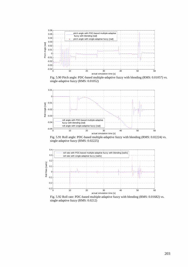
203
0 10 20 30 40 50 60-0.04
-0.03
-0.02
-0.01
0
0.01
0.02
0.03
0.04
0.05
0.06
actual simulation time [s]
Pitc
h A
ngle
[ra
d]
pitch angle with PDC-based multiple-adaptive fuzzy with blending [rad]
pitch angle with single-adaptive fuzzy [rad]
Fig. 5.90 Pitch angle: PDC-based multiple-adaptive fuzzy with blending (RMS: 0.01057) vs. single-adaptive fuzzy (RMS: 0.01052)
0 10 20 30 40 50 60-0.05
-0.04
-0.03
-0.02
-0.01
0
0.01
actual simulation time [s]
Rol
l Ang
le [
rad]
roll angle with PDC-based multiple-adaptive fuzzy with blending [rad]
roll angle with single-adaptive fuzzy [rad]
Fig. 5.91 Roll angle: PDC-based multiple-adaptive fuzzy with blending (RMS: 0.02224) vs. single-adaptive fuzzy (RMS: 0.02225)
0 10 20 30 40 50 60-0.3
-0.2
-0.1
0
0.1
0.2
0.3
0.4
actual simulation time [s]
Rol
l Rat
e [r
ad/s
]
roll rate with PDC-based multiple-adaptive fuzzy with blending [rad/s]
roll rate with single-adaptive fuzzy [rad/s]
Fig. 5.92 Roll rate: PDC-based multiple-adaptive fuzzy with blending (RMS: 0.01682) vs. single-adaptive fuzzy (RMS: 0.0212)
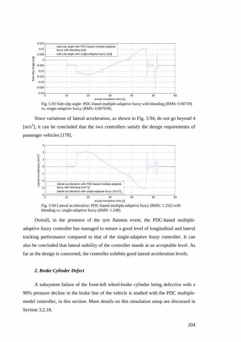
204
0 10 20 30 40 50 60-0.03
-0.025
-0.02
-0.015
-0.01
-0.005
0
0.005
0.01
0.015
actual simulation time [s]
Sid
e-S
lip A
ngle
[ra
d]
side-slip angle with PDC-based multiple-adaptive fuzzy with blending [rad]
side-slip angle with single-adaptive fuzzy [rad]
Fig. 5.93 Side-slip angle: PDC-based multiple-adaptive fuzzy with blending (RMS: 0.00719) vs. single-adaptive fuzzy (RMS: 0.007039)
Since variations of lateral acceleration, as shown in Fig. 5.94, do not go beyond 4
[m/s2], it can be concluded that the two controllers satisfy the design requirements of
passenger vehicles [178].
0 10 20 30 40 50 60-4
-3
-2
-1
0
1
2
3
actual simulation time [s]
Late
ral A
ccel
erat
ion
[m/s
2 ]
lateral acceleration with PDC-based multiple-adaptive fuzzy with blending [m/s 2]
lateral acceleration with single-adaptive fuzzy [m/s 2]
Fig. 5.94 Lateral acceleration: PDC-based multiple-adaptive fuzzy (RMS: 1.252) with blending vs. single-adaptive fuzzy (RMS: 1.248)
Overall, in the presence of the tyre flatness event, the PDC-based multiple-
adaptive fuzzy controller has managed to ensure a good level of longitudinal and lateral
tracking performance compared to that of the single-adaptive fuzzy controller. It can
also be concluded that lateral stability of the controller stands at an acceptable level. As
far as the design is concerned, the controller exhibits good lateral acceleration levels.
2. Brake Cylinder Defect
A subsystem failure of the front-left wheel-brake cylinder being defective with a
90% pressure decline in the brake line of the vehicle is studied with the PDC multiple-
model controller, in this section. More details on this simulation setup are discussed in
Section 3.2.18.

205
The tracking performances of the PDC multiple-model adaptive fuzzy controller
have been significant with regard to longitudinal and lateral tracking aspects as shown
in Figs. 5.95–5.96, in comparison to that of the single-adaptive fuzzy controller.
0 10 20 30 40 50 60-2
0
2
4
6
8
10
12
14
actual simulation time [s]
Long
itudi
nal E
rror
[m
]
longitudinal error with PDC multiple-adaptive fuzzy with blending [m]
longitudinal error with single-adaptive fuzzy [m]
Fig. 5.95 Longitudinal error: PDC-based multiple-adaptive fuzzy with blending (RMS: 3.062) vs. single-adaptive fuzzy (RMS: 3.159)
0 10 20 30 40 50 60-0.1
0
0.1
0.2
0.3
0.4
actual simulation time [s]
Late
ral E
rror
[m
]
lateral error with single-adaptive fuzzy [m]
lateral error with PDC multi-adaptive fuzzy [m]
Fig. 5.96 Lateral error: PDC-based multiple-adaptive fuzzy with blending (RMS: 0.007504) vs. single-adaptive fuzzy (RMS: 0.03453)
Pitch angle variation, normally a longitudinal stability measure as shown in Fig.
5.97 for both controllers, has been similar.
0 10 20 30 40 50 60-0.04
-0.03
-0.02
-0.01
0
0.01
0.02
0.03
0.04
actual simulation time [s]
Pitc
h A
ngle
[ra
d]
pitch angle with single-adaptive fuzzy [rad]
pitch angle with PDC multi-adaptive fuzzy [rad]
Fig. 5.97 Pitch angle: PDC-based multiple-adaptive fuzzy with blending (RMS: 0.01574) vs. single-adaptive fuzzy (RMS: 0.01583)

206
The variations of roll angle, roll rate and side-slip angle, as shown in Figs. 5.98–
5.100, for the PDC multiple-controller are within the same range as that for the single-
adaptive fuzzy controller. There are some high-valued areas too, in relation to the PDC
multiple-model controller. Since these values are still within the range suggested by the
single-adaptive fuzzy controller, the lateral stability levels exercised by the PDC
multiple-adaptive fuzzy controller are acceptable.
0 10 20 30 40 50 60-0.04
-0.03
-0.02
-0.01
0
0.01
0.02
0.03
actual simulation time [s]
Rol
l Ang
le [
rad]
roll angle with PDC multi-adaptive fuzzy[rad]
roll angle with single-adaptive fuzzy[rad]
Fig. 5.98 Roll angle: PDC-based multiple-adaptive fuzzy with blending (RMS: 0.01069) vs. single-adaptive fuzzy (RMS: 0.01082)
0 10 20 30 40 50 60-0.5
-0.4
-0.3
-0.2
-0.1
0
0.1
0.2
0.3
0.4
actual simulation time [s]
Rol
l Rat
e [r
ad/s
]
roll rate with PDC multi-adaptive fuzzy [rad/s]
roll rate with single-adaptive fuzzy [rad/s]
Fig. 5.99 Roll rate: PDC-based multiple-adaptive fuzzy with blending (RMS: 0.04591) vs. single-adaptive fuzzy (RMS: 0.04617)

207
0 10 20 30 40 50 60-0.07
-0.06
-0.05
-0.04
-0.03
-0.02
-0.01
0
0.01
0.02
0.03
actual simulation time [s]
Sid
e S
lip A
ngle
[ra
d]
side slip angle with single-adaptive fuzzy [rad]
side slip angle with PDC multi-adaptive fuzzy [rad]
Fig. 5.100 Side-slip angle: PDC-based multiple-adaptive fuzzy with blending (RMS: 0.009642) vs. single-adaptive fuzzy (RMS: 0.01052)
As far as lateral acceleration is concerned, as shown in Fig. 5.101, the variation
exhibited by the PDC multiple-model adaptive fuzzy controller is nearly around 4
[m/s2] in the extreme. But, in comparison to the performance by the single-adaptive
fuzzy controller, the PDC multiple-model controller shows an exceptional
improvement. It can be said that the values of the PDC multiple-adaptive fuzzy
controller remain within the design requirements of passenger vehicles, with a slight
drift towards the ‘transition range’ [178], though.
0 10 20 30 40 50 60-20
-15
-10
-5
0
5
10
actual simulation time [s]
Late
ral A
ccel
erat
ion
[m/s
2 ]
lateral acceleration with single-adaptive fuzzy [m/s 2]
lateral acceleration with PDC multi-adaptive fuzzy [m/s 2]
Fig. 5.101 Lateral acceleration: PDC-based multiple-adaptive fuzzy with blending (RMS: 1.341) vs. single-adaptive fuzzy (RMS: 1.334)
Overall, in the presence of a brake cylinder pressure failure, the PDC multiple-
model adaptive fuzzy controller has shown to exhibit significant improvements in
lateral and longitudinal tracking performances in relation to the single-adaptive fuzzy
controller. As suggested by variations of side-slip angle, roll-angle and roll rate, the
lateral stability performance of the PDC controller can be said to be slightly superior to
that of the single-adaptive fuzzy controller.
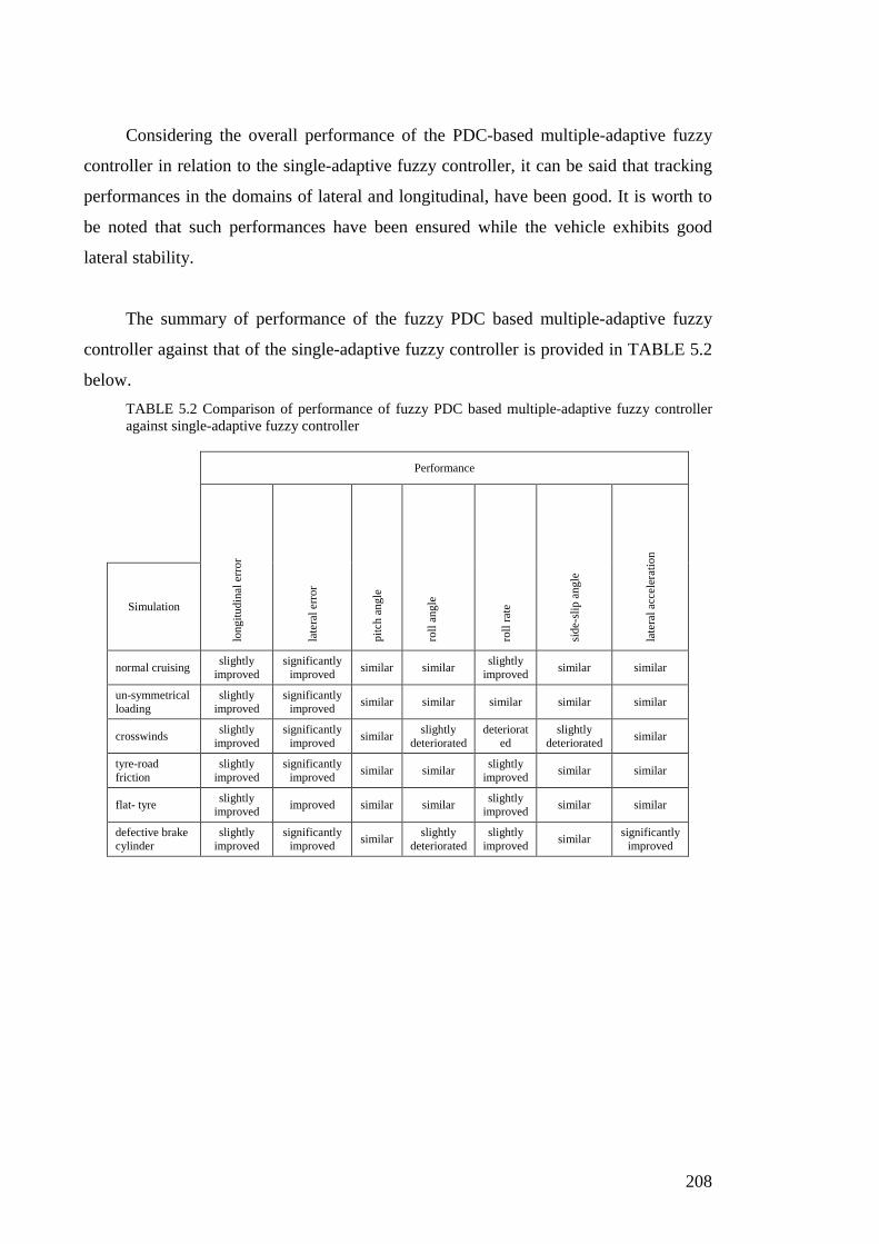
208
Considering the overall performance of the PDC-based multiple-adaptive fuzzy
controller in relation to the single-adaptive fuzzy controller, it can be said that tracking
performances in the domains of lateral and longitudinal, have been good. It is worth to
be noted that such performances have been ensured while the vehicle exhibits good
lateral stability.
The summary of performance of the fuzzy PDC based multiple-adaptive fuzzy
controller against that of the single-adaptive fuzzy controller is provided in TABLE 5.2
below.
TABLE 5.2 Comparison of performance of fuzzy PDC based multiple-adaptive fuzzy controller against single-adaptive fuzzy controller
Performance
Simulation
long
itudi
nal e
rror
late
ral e
rror
pitc
h a
ngle
roll
ang
le
roll
rate
side
-slip
ang
le
late
ral a
cce
lera
tion
normal cruising slightly
improved significantly
improved similar similar
slightly improved
similar similar
un-symmetrical loading
slightly improved
significantly improved
similar similar similar similar similar
crosswinds slightly
improved significantly
improved similar
slightly deteriorated
deteriorated
slightly deteriorated
similar
tyre-road friction
slightly improved
significantly improved
similar similar slightly
improved similar similar
flat- tyre slightly
improved improved similar similar slightly
improved similar similar
defective brake cylinder
slightly improved
significantly improved
similar slightly
deteriorated slightly
improved similar
significantly improved

209
5.3 Chapter Summary
In this chapter, the development of two robust multiple-model/multiple-adaptive
controllers based on soft-switching (blending) is described.
Firstly, a robust multiple-adaptive fuzzy controller with blending is synthesized. A
similar procedure to developing the single-adaptive fuzzy controller is followed in
tuning the individual adaptive fuzzy controllers in the multiple-adaptive setup. In the
design of the fuzzy blender, for determining the fixed parameters, a number of vehicle
runs are conducted and data gathered. Using this data, with the subtractive clustering
and ANFIS methods, parameters for the fuzzy blender are found. A detailed robust
stability analysis procedure is followed for ensuring asymptotic stability of the system
using a Lyapunov based KYP lemma. The developed controller is validated using a
comprehensive set of simulations on veDYNA®. These simulations include testing of
the controller under a number of external disturbances as well as a couple of failure
modes.
Secondly, a robust PDC-based multiple-model adaptive fuzzy controller is
synthesized comprehensively. In designing an implementation level PDC-based
controller, a comprehensive sector nonlinearity method is used to construct the local
models and local adaptive fuzzy controllers. Once again a detailed robust stability
analysis procedure is followed for ensuring asymptotic stability of the general PDC-
based system using the Lyapunov based KYP lemma. The developed controller is
validated using a comprehensive set of simulations on veDYNA®. These simulations
also include the testing of the controller under a number of external disturbances as well
as a couple of failure modes.

210

211
C H A P T E R 6
Robust Multiple-Adaptive Fuzzy Control Systems – Switching (Hard-Switching) This chapter describes a design of a multiple-adaptive fuzzy controller based on
‘switching’ (more specifically termed as ‘hard-switching’) for addressing the problem
of integrated lateral and longitudinal control of vehicles. The resulting controller is a
‘binary’ switching structure consisting of a bank of adaptive fuzzy controllers. In the
design of the MM/MC based adaptive fuzzy controller with switching, a comprehensive
investigation of stability is carried out using a Lyapunov based KYP lemma leading to
asymptotic stability. In the validation of the designed ‘switching’ based control system,
two separate simulations are carried out. The first simulation is included with ‘two’
number of adaptive fuzzy controllers (AFCs), while the second is included with ‘four’
adaptive fuzzy controllers, in the multiple-adaptive fuzzy setup. These two simulations
are used to demonstrate the effects of having different number of adaptive fuzzy
controllers in the switching based MM/MC structure.

212
6.1 Robust Multiple-Adaptive Fuzzy Control Systems with Switching (Hard-Switching)
6.1.1 Introduction
There are drawbacks of using single-model (or single ‘modal’) control systems in
addressing the problem of integrated lateral and longitudinal control of highway
vehicles. This issue has already been discussed in the main introduction.
But, MM/MC systems provide a solution in the multiple-environments of
operation of vehicles, which overcomes the drawbacks that associate with the single-
model control systems.
It is customary to define a particular generic scenario as a combination of sub-
scenarios. For such occasions, there is little doubt that ‘blending’ based controllers are
more appropriate. But, when the scenarios become more specifically defined, the most
appropriate solution would be to have a ‘dedicated’ controller selected from a bank of
controllers with ‘switching’ (binary selection). In this regard, the need of a ‘switching’
controller in the context of MM/MC setup arises when a particular scenario requires a
specific controller without combining it with any other controller in the bank in
addressing the problem of vehicle control. This chapter provides a design of a robust
multiple-adaptive fuzzy controller based on switching for addressing the problem of
integrated lateral and longitudinal control of vehicles.
This robust multiple-adaptive fuzzy controller (as a multiple-model method) with
switching is more versatile in comparison to linear multiple-model control systems due
to the inclusion of adaptive fuzzy controllers [20]. This inclusion substantially pays off
with the fact that it is possible to program the adaptive fuzzy controllers in a versatile
manner in accordance with complex scenarios. In addition, having adaptive fuzzy
control functions enables one to define and model ‘uncertainty’ of the system over
which the control action is executed.

213
6.1.2 Synthesis of Robust Multiple-Adaptive Fuzzy Controller with Switching
In this section, the design of a novel setup of robust multiple-adaptive fuzzy
controllers based on switching is described. In this controller setup, a number of
adaptive fuzzy controllers are included in the multiple-adaptive fuzzy system. These
adaptive fuzzy controllers are designed based on possible scenarios the vehicle system
is expected to be exposed to. The adaptive rates of each adaptive controller in the
controller bank are made different from each other to allow for different scenarios. In
other words, a higher adaptive rate allows for fast dynamical changes while a lower
adaptive rate allows for slow changes. This is the general set up of the multiple-adaptive
fuzzy controller that will follow.
In the normal setup, adaptive fuzzy controllers are trained in the normal operating
conditions. The scope of the multiple-adaptive fuzzy controller with switching can be
extended to include fault conditions for some selected vehicle sub-components. This
extension will introduce more versatility to the system. Identification of different fault
conditions can be done with predefined residuals [180]. But, this extended usage is not
covered in this research.
In the designed controller setup, the switching system activates to select the
particular adaptive fuzzy controller that is the most suitable to be connected to the
vehicle at a time. The selection of one of these controllers is based on the minimum
value of a pre-defined cost function. The switching is carried out in a similar way to the
well-established MMST (Multiple-Model Switching and Tuning) method [31]. But, the
main difference is that the proposed method in this section allows switching of more
complicated and versatile adaptive fuzzy controllers rather than linear controllers (the
mostly used form in the MMST method). The other difference from the MMST method
is that the proposed method does not need different vehicle models being defined in the
aid of switching.
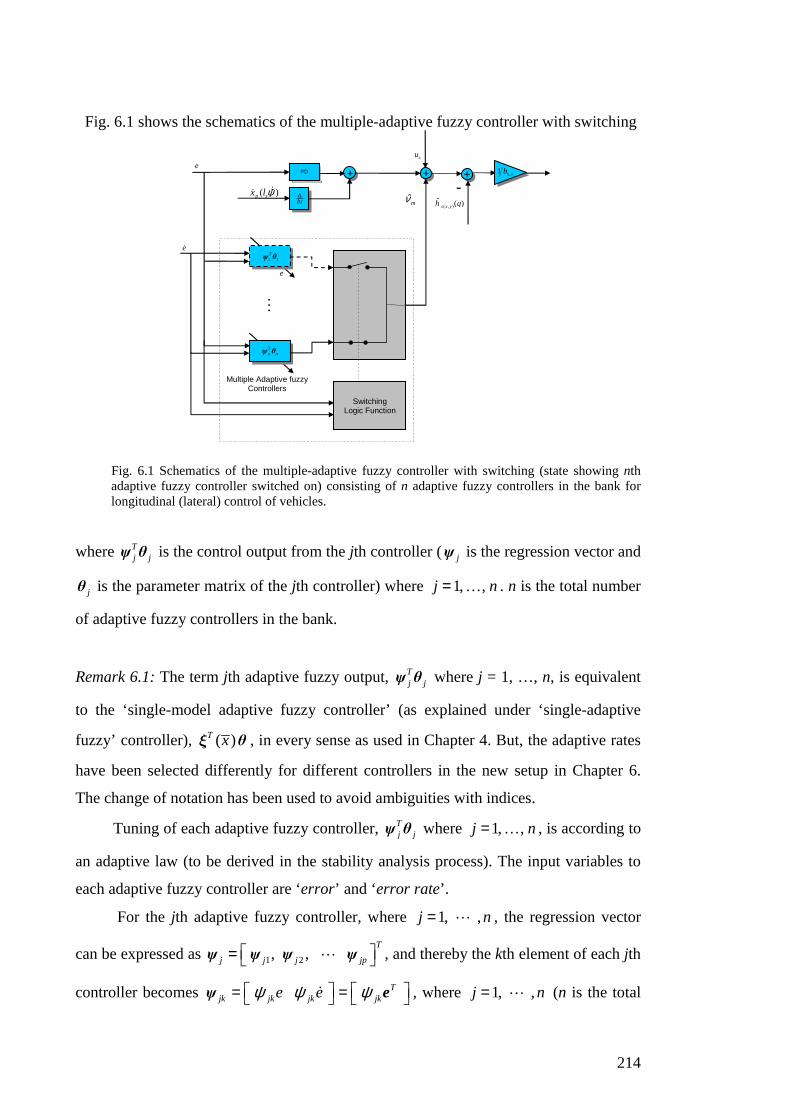
214
Fig. 6.1 shows the schematics of the multiple-adaptive fuzzy controller with switching
Fig. 6.1 Schematics of the multiple-adaptive fuzzy controller with switching (state showing nth adaptive fuzzy controller switched on) consisting of n adaptive fuzzy controllers in the bank for longitudinal (lateral) control of vehicles.
where Tj jψ θ is the control output from the jth controller ( jψ is the regression vector and
jθ is the parameter matrix of the jth controller) where 1, ,j n= … . n is the total number
of adaptive fuzzy controllers in the bank.
Remark 6.1: The term jth adaptive fuzzy output, Tj jψ θ where j = 1, …, n, is equivalent
to the ‘single-model adaptive fuzzy controller’ (as explained under ‘single-adaptive
fuzzy’ controller), ( )T x θξ , in every sense as used in Chapter 4. But, the adaptive rates
have been selected differently for different controllers in the new setup in Chapter 6.
The change of notation has been used to avoid ambiguities with indices.
Tuning of each adaptive fuzzy controller, Tj jψ θ where 1, ,j n= … , is according to
an adaptive law (to be derived in the stability analysis process). The input variables to
each adaptive fuzzy controller are ‘error’ and ‘error rate’.
For the jth adaptive fuzzy controller, where 1, ,j n= ⋯ , the regression vector
can be expressed as 1 2, ,T
j j j jp = ψ ψ ψ ψ⋯ , and thereby the kth element of each jth
controller becomes Tjk jk jk jke eψ ψ ψ = = ψ eɺ , where 1, ,j n= ⋯ (n is the total
su PD
⋮
e
e
-
eɺ
Multiple Adaptive fuzzy Controllers
( )p sx l ɺɶɺ ψ ˆmν
ˆ ( )h xɺ
( , )ˆ ( )s x yh q
Switching
Logic Function
,1 x yb
1 1Tψ θ
Tn nψ θ
s
t∆∆
+ + +
215
number of controllers in the bank), and 1, ,k p= ⋯ . Here, p is the total number of IF-
THEN fuzzy rules in each individual adaptive fuzzy controller.
The output membership function parameter set of each adaptive fuzzy controller
can be tuned using an algorithm based on an adaptive law. For the jth adaptive fuzzy
controller, the adaptive law can be expressed as
j j jγ= −θ ψ Ceɺɶ (6.1)
where 1, ,j n= ⋯ , for n number of adaptive fuzzy controllers.
(i) Control Law
The certainty equivalence control laws can be obtained
for longitudinal control as
1 ˆˆ ( )Tx p dx x px x j j sx x sx
x
u x k e k e u h qb = + + + + −
ψ θɺɺ ɺ ɺ , (6.2)
and for lateral control as
1 ˆˆ ( )s
Ty s dy y py y j j sy y sy
y
u l k e k e u h qb
ψ = + + + + − ψ θɺɺɶ ɺ ɺ . (6.3)
Remark 6.2: Though fuzzy systems in (6.2), (6.3) are generally nonlinear, each is linear
with respect to its unknown parameters. Hence, parameter adaptation algorithms
applicable for linear systems, e.g. gradient-based algorithms, can be readily used in
estimation of the unknown parameters in fuzzy systems in (6.2), (6.3) [27].
The switching system to be described, selects the most suitable adaptive fuzzy
controller from the bank of adaptive fuzzy controllers (for jth controller, it is Tj jψ θ
where 1, ,j n= ⋯ ), and connects it to the output. Each 1 2, , , nθ θ θ⋯ provides the set of
parameter matrices for each adaptive fuzzy controller.

216
(ii) Error Dynamics
The equation (6.2) can be substituted in (3.4)–(3.6), and will result in
for longitudinal dynamics
*
ˆ ( ) ( )
ˆ
,
Tx dx x px x x s x s j j sx xx
x x x sx x
x sx x
e k e k e h q h q u d
w u d
u d
ν ν
ν
+ + = − − − −
= + − − −
= − −
ψ θɺɺ ɺ ɺ ɺ
ɶ
(6.4)
and for lateral error dynamics
*
ˆ ( ) ( )
ˆ
.
s s
Ty dy y py y y s y s j j sy yy
y y y sy y
y sy y
e k e k e h q h q u d
w u d
u d
ν ν
ν
+ + = − − − −
= + − − −
= − −
ψ θɺɺ ɺ ɺ ɺ
ɶ
(6.5)
Here, ,ˆ ( )
sx y sh qɺ denotes the calculated value of the term , ( )sx y sh qɺ , true vehicle
dynamics. ˆxν and ˆyν are the outputs from the selected adaptive fuzzy controller for
longitudinal and lateral cases, respectively. dxk , pxk are the constant PD (proportional-
derivative) gains for the longitudinal control and dyk , pyk are the constant PD gains for
the lateral control. s sx syu u u = is the variable structure control term.
In this discussion, * * *x yν ν ν = is the optimal adaptive fuzzy output while
ˆ ˆ ˆx yν ν ν = is the actual adaptive fuzzy output. xw , yw are the adaptive fuzzy
approximation errors, and are bounded by x xw W< and y yw W< . xW , yW ( > 0)∈R
are the practical bounds.
By using the universal approximation theorem (provided in Chapter 4), with the
fuzzy adaptation process, the fuzzy controller parameters can be gradually brought to
optimal values, and thus the right half of the equations, (6.2) and (6.3) can be made
zero.

217
In this case, the variable structure term, su is used to dissipate the effects of fuzzy
approximation errors, and to some extent the disturbances. The overall uncertainty
factor in the equation is made zero with the fuzzy function.
(iii) Training of Multiple-Adaptive Fuzzy System
The set of adaptive fuzzy controllers can be used in two different ways with
effectiveness. First, each adaptive fuzzy controller can be trained with the same data set
(obtained from running a vehicle through a real scenario) to obtain its input and output
membership parameters. Then the adaptive rates in the adaptive law can be changed to
differentiate each controller from another. The adaptive fuzzy controllers having ‘higher
adaptive rate’ can be used to make use of the faster changing scenarios while the
controllers having ‘lower adaptive rate’ can be used to catch up with the low frequency
changes in the scenarios. This is the procedure adopted in the rest of the section.
Even though it is not followed, another option can also be considered. Instead of
having a common data set for the fuzzy system, the data space can be categorized into
groups, e.g., according to the frequency of the variable ‘error’. Using each of the ‘local’
data set, each adaptive fuzzy controller can be trained. The ‘best’ adaptive fuzzy
controller for the task can be selected according to the switching criteria.
The following procedure was adopted for tuning the multiple-adaptive fuzzy system
based on switching:
(i) The subtractive clustering method was used to obtain the preliminary fuzzy
membership function centres and standard deviations (Gaussian), and then the basic
structure was further trained with ANFIS using gathered data from veDYNA®.
(ii) The individual adaptive fuzzy controller systems are based on the design of Section
4.3, and thereafter different adaptive rates are added for individual controllers.

218
6.1.3 Stability Analysis of Control System
(i) Switching Function Characteristics
The switching function characteristics of the controller can be described as
follows. The magnitude of the adaptation function of the jth adaptive fuzzy controller
can be taken as
j j jγ= ψ Ceεεεε (6.6)
where 1,...,j n= . This function can be described as an overall indicator for determining
how much the particular adaptive fuzzy controller in the bank, i.e. jth controller, adapts.
In other words, this ‘magnitude’ of the function provided by (6.6) is a measure of how
much the particular controller drifts from the present status. The argument here is that
the larger the amount of drift from the present status, the more likely it is away from the
required present ‘state’. In other words, if a controller has to work out a larger change to
adapt to the next stage, it can be taken as less suitable in the selection procedure. For
more reliability of selection, the magnitude of the adaptation function is used to define a
cost function, and the value of the cost function is used for determining the best
controller for the task.
Definition 6.1: The cost function based on adaptation for the jth adaptive fuzzy
controller can be defined as 22
1 2 0
t
j j jJ κ ε κ ε= + ∫ɺ , where 1,...,j n= .
(ii) Stability Analysis of Multiple-Adaptive Fuzzy Control with Switching
The following stability proof of the multiple-adaptive fuzzy control system with
switching is done for the generic case irrespective whether it is lateral or longitudinal
controller. Therefore, the subscripts that are specific to either longitudinal or lateral case
are removed in this description. Nevertheless, the specific details will be mentioned as
and when necessary.

219
Assumption 6.1: The sum of fuzzy approximation errors,w is bounded, i.e.,
w W≤ where ( 0)W > ∈R . The external disturbances, d are bounded too, i.e.,
d D≤ where ( 0)D > ∈R . Thereby the variable structure control gain is chosen as
f W Dσ ≥ + .
The following assumptions are made to ascertain the switching, and thereby to ensure
stability properties.
Assumptions 6.2: The assumptions made on switching are:
(C.1) The active controller, i.e., kth adaptive fuzzy controller, is selected at a particular
time according to the criterion 1, ... ,mink jj n
J J=
= , 1, ... ,k n∈ and 1,...,j n= .
(C.2) Let the timing sequence for switching be 1 2, , ,S t t t∞= … , and let qt be any
time of typical switching, where 1, 2, ,q = ∞… . Then it is always ensured
1 0q qt t t+ ≥ + where 0 0t > is the minimum time gap for two consecutive switching cases
enforced to avoid an infinite switching to occur at a time. The decision for choosing 0t
is based on optimum control performance of the system.
The main features of the robust multiple-adaptive fuzzy control with switching
can be summarized in the following theorem.
Theorem 6.1: Let the parameter vectors, jθ of the adaptive fuzzy systems be adjusted
by the adaptive law as provided in (6.1) and let Assumptions 6.1 and 6.2 be true. The
proposed adaptive fuzzy control law as provided in (6.2) [and (6.3)] can guarantee
stability of the vehicle system with the following properties:
i) The closed loop vehicle system is stable, i.e. ∈e ∞L (considering both lateral and
longitudinal cases).
ii) The system errors and all the control system parametric errors are asymptotically
stable, i.e. lim 0t x ye , e→∞ = and lim 0t jθ→∞ =ɶ (considering both lateral and longitudinal
cases) where 1,...,j n= .

220
Proof:
Positive realness of the transfer function of error dynamics equation, i.e., (4.23)
and (4.24), related to vehicle dynamics has already been established in Section 4.2.6.
Assuming positive realness of the vehicle error dynamics can be established as
shown in Section 4.2.6, according to Kalman–Yakubovich–Popov (KYP) lemma [175]
for a strictly positive-real system, there exist two positive definite matrices P and Q
(i.e., 0T= >P P and 0T= >Q Q ) satisfying
T + + =A P PA Q 0, and T=PB C . (6.7)
Now, the following Lyapunov function can be defined as (for lateral or longitudinal
system)
1T Tj j jV γ −= +e Pe θ θɶ ɶ (6.8)
where 0T= >P P . And ( ) 0jγ ∈ >R is a constant. Here e is the overall system error
vector and jθɶ is the parametric error vector for the jth adaptive fuzzy controller, where
1,...,j n= , of the bank of controllers.
Lyapunov candidate as provided in (6.8) quantifies both in tracking error and in
parameter estimates. Differentiating the Lyapunov function along the trajectories of the
error system will provide
( )1 1 .T T T Tj j j j j jV γ γ− −= + + +e Pe e Pe θ θ θ θɺ ɺɶ ɶ ɶ ɶɺ ɺ ɺ (6.9)
Substituting for eɺ from the equation (4.23), it will provide
( )1 1( ) ( ) .T T T Ts s j j j j j jV d u d uν ν γ γ− −= + − − + + − − + +Ae B B B Pe e P Ae B B B θ θ θ θ
ɺ ɺɶ ɶ ɶ ɶɺ ɶ ɶ
(6.10)
Rearranging (6.10) will provide
( )1 1
( )
.
T T T T T T T T Ts s
T Tj j j j j j
V d d u uν ν
γ γ− −
= + + + − − − −
+ +
e A P PA e B Pe e PB B Pe e PB B Pe e PB
θ θ θ θ
ɺ ɶ ɶ
ɺ ɺɶ ɶ ɶ ɶ
(6.11)

221
By substitution of the Lyapunov equation 0T + + =A P PA Q , where 0T= >Q Q ,
equation (6.11) can be further simplified as
( )( ) ( )1 1
1.
nT T T T T T T Ts j j j j j jj
V d uν ν γ γ− −=
= − + + − + + + +∑e Qe B Pe e PB B Pe e PB θ θ θ θɺ ɺɶ ɶ ɶ ɶɺ ɶ ɶ
(6.12)
From the argument, it can be expressed as * ˆ( )ν ν ν τ= − +ɶ . It can be further elaborated
that
* ˆT Tj j j j jwν = − +ψ θ ψ θɶ (6.13)
where * 2pj
×∈θ R is the optimal parameter matrix. p is the total number of IF-THEN
fuzzy rules in each individual adaptive fuzzy controller. ˆjθ is the parameter set of jth
controller, and jw is the fuzzy approximation error of the jth adaptive fuzzy controller.
jw is bounded, jw W≤ where jw ∞∈L . And W ∈R is a positive constant. The
determination of fuzzy approximation error upper bound, W has been discussed before
[30].
Equation (6.13) can be further simplified so that
* ˆ( )Tj j j jwν = − +ψ θ θɶ . (6.14)
Let the parameter error be taken as * ˆj j j= −θ θ θɶ . Equation (6.14) now becomes
.Tj j jwν = +ψ θɶɶ (6.15)
Substituting (6.15) in (6.12) will become
( ) ( )( )( ) ( )1 1 .
TT T T T Tj j j j j j
T T T Ts j j j j j j
V w w
d u γ γ− −
= − + + + +
− + + + +
e Qe ψ θ B Pe e PBψ θ
B Pe e PB θ θ θ θ
ɶ ɶɺ
ɺ ɺɶ ɶ ɶ ɶ (6.16)
Since T=PB C , (6.16) can be further simplified to provide
( ) ( )( )1 1 .
T T T T Tj j j j
T T T Tj j j j j j j s
V
w d uγ γ− −
= − + +
+ + + − − +
e Qe θ ψ Ce e Cψ θ
θ θ θ θ Ce e C
ɶ ɶɺ
ɺ ɺɶ ɶ ɶ ɶ (6.17)
Further rearrangement of (6.17) will result in
222
( )( ) ( )( )
1
1 .
T T T T Tj j j j
T T Tj j j j j s
V
w d u
γ
γ
−
−
= − + +
+ + + − − +
e Qe e Cψ θ θ
θ ψ Ce θ Ce e C
ɺɶ ɶɺ
ɺɶ ɶ (6.18)
Now, (6.18) can be written as
( )( ) ( )( )
1
1 .
TT
j j j j
T T Tj j j j j s
V
w d u
γ
γ
−
−
= − + +
+ + + − − +
e Qe ψ Ce θ θ
θ ψ Ce θ Ce e C
ɺɶ ɶɺ
ɺɶ ɶ (6.19)
At any moment of time, it is taken as j j jγ= −θ ψ Ceɺɶ for j∀ . Thereby (6.19) further
simplifies to (with reference to the conditional assumptions C.1 and C.2)
( )( )T T Tj sV w d u= − + − − +e Qe Ce e Cɺ . (6.20)
Equation (6.20) can be further expressed as
( )( )2
minT T
j sV w d uλ≤ − + − − +Q e Ce e Cɺ , (6.21)
where minλQ is the minimum eigen value of Q .
Since fuzzy systems follow universal approximation theorem [29], jw may be made
arbitrarily small, thereby making each jw small by proper choice of each adaptive fuzzy
system if each Tj j jν =ψ θ is smooth (note that this may require an arbitrarily large
number of rules for each controller) [30].
Since jw W≤ , and d D≤ , (6.21) can be further written as
( )( )2
minT T
sV D W uλ≤ − + + − +Q e Ce e Cɺ . (6.22)
Let the variable structure control term be
( )T Ts fu signσ= +Ce e C , (6.23)
and thereby (6.22) can be further expressed as
( )2
minT T
fV D Wλ σ≤ − + + − +Q e Ce e Cɺ . (6.24)

223
Further rearrangement of (6.24) will provide
( )2
minT T
fV D Wλ σ≤ − − + − +Q e Ce e Cɺ . (6.25)
If it is taken as
f D Wσ ≥ + , (6.26)
then (6.25) will establish that
0V ≤ɺ , t∀ . (6.27)
Therefore, according to Lyapunov theory, it establishes the fact that e is bounded,
i.e. ∞∈e L . Therefore, ,e eɺ are bounded, i.e. ,e e ∞∈ɺ L . It also establishes that
parameter errors are bounded, i.e. j∞∈θɶ L where 1,...,j n= .
Equation (6.25) also implies that
2
minV λ≤ − Q eɺ . (6.28)
Integrating (6.28) will provide
2
min 0 0(0) ( )dt Vdt V Vλ
∞ ∞≤ − = − ∞∫ ∫Q e ɺ . (6.29)
Therefore, (6.29) becomes
( )min
2 1
0(0) ( )dt V Vλ
∞≤ − ∞∫ Q
e . (6.30)
Equation (6.30) leads to
2∈e L 2 2
0( ) : ( )z t z t dt
∞ = < ∞ ∫L , (6.31)
since it provides (0), ( )V V ∞∞ ∈L according to (6.27) [30]. Since it is possible to
establish as 2e ∞∈L L∩ (from (6.31) and (6.27)), and e ∞∈ɺ L (from (6.28)) by
Barbalat’s lemma [30], [176], it can be established with asymptotic stability of e (i.e.
lim 0t e→∞ = ). This result of asymptotic stability can be extended specifically to lateral
and longitudinal cases, and consequently the lateral and longitudinal errors are
asymptotically stable, i.e.
lim 0.t x ye , e→∞ = (6.32)
This asymptotic stability result as provided by (6.32) proves that when lateral and
longitudinal cases are considered at the same time, with the above arguments, the

224
system of errors can be proved to be asymptotically stable. Therefore, this result
logically proves the integrated lateral and longitudinal control system is asymptotically
stable. This statement completes the proof of stability for the robust multiple-adaptive
fuzzy system with switching.
Remark 6.3: The Lyapunov candidate as provided in (6.8) satisfies the conditions
i) V is at least 1C
ii) (0) 0V = and ( ( )) 0V x t > for ( ) 0x t ≠ and
iii) ( ) ( ( ))x t V x t→ ∞ ⇒ → ∞ .
( ( )x t denotes a selected time-dependent state of the system in this remark).
The following definition is provided to formerly identify the variable vector spaces and
thereby to define the optimal parameter set.
Definition 6.2: The compact parameter spaces for jθ and x variables can be defined.
Let ( 0)Mθ > ∈R and ( 0)xM > ∈R be finite, and it provide
:j j j Mθ = ∈ ≤
θΩ θ θR , and
:x xx x M= ∈ ≤Ω R .
Thereby the optimal parameter set for each jth adaptive fuzzy controller where j = 1, …
, n, can be formally defined as
* * ˆarg min supj x
Tj j j
xθ
ν∈ ∈
= − θ Ω Ω
θ ψ θ (6.33)
where *ν is the optimal adaptive fuzzy function output, and *ν ∈R . x is the generic
input variable to each fuzzy system.
Remark 6.4: The definition of *jθ is only for theoretical reasons, and therefore it is not
required for implementation of the controller.
The following features can be observed with regard to the switching scheme
established for selecting the best adaptive fuzzy controller at a time. Since all adaptive
fuzzy controller models have been proved as asymptotically stable, the switching
scheme is not critical [116]. Since the overall system is ensured with finite switching, it
is guaranteed to prevent from chattering [22]. Since there is a minimum timing gap

225
between every consecutive switching in the sequence, it can be called a permissible
switching scheme [22]. These permissible switching schemes prevent infinite switching.
The dynamics of the system during the switching period can be analysed as follows. In
a typical switching setup when the controller switches from one controller to a different
controller based on the provided conditions, there is a natural tendency to increase
undesired transients or ‘bumps’ in the control output signal [181]. When the switching
scheme of this research is considered while the adaptive fuzzy controllers are switched
between, the PD module remains as the ‘coarse-tuning controller’ every time. What is
really switched between is the module that addresses fine-tuning, i.e. adaptive fuzzy
controller. In other words, the switched controllers occur in the ‘secondary-layer’, i.e.
adaptive fuzzy controllers, while the ‘primary-layer’, i.e. PD module, remains in control
every time. This is in contrast to that occurs in MMST method where the main
controllers operate in the ‘primary-layer’ are switched [31]. Based on these facts it can
emphatically say that the transients or ‘bumps’ that occur in the switching systems in
this research are far less in comparison to that in the MMST method. In other words, the
switching controllers proposed in this research can be said to be much closer to ‘bump-
less’ switching controllers than that use the MMST method [182].

226
6.1.4 Simulation Studies, Results and Discussion for ‘Two’ Adaptive Fuzzy Controllers in the Bank (Multiple-Adaptive Fuzzy Controller with Switching)
In this simulation, the developed robust multiple adaptive fuzzy controller with
switching was included with ‘two’ adaptive fuzzy controllers in the bank for each
longitudinal and lateral controller.
(i) Simulation Setup
The simulation setup for this section was similar to the one provided in Chapter 4
for single-adaptive fuzzy controller system, except for the facts otherwise stated in this
section. The simulation setup included veDYNA® setup, simulation profile details and
other settings.
In this simulation, the multiple-adaptive fuzzy controller with switching was
included with two adaptive fuzzy controllers in the bank. Therefore, the adaptive gains
were taken as 1 0.03xγ = , 2 0.04xγ = for longitudinal, and 1 0.01yγ = , 2 0.03yγ = for
lateral cases, for each adaptive fuzzy controller in the bank. This change in the range in
adaptive gains is due to the fact that lateral dynamics changes at comparatively low rate
than the longitudinal.
(ii) Simulation Results and Discussion
In the following figures depicting simulation results, each performance parameter
of the multiple-adaptive fuzzy controller with switching (solid blue line) is compared
against that of the single-adaptive fuzzy controller (dotted red line).

227
(a) Normal Cruising Conditions: Multiple-Adaptive Fuzzy Control with Switching (2-AFCs)
The following simulation results illustrate the performance of the developed
multiple-adaptive fuzzy controller (with two adaptive controllers in the bank) with
switching, as against the performance of single-adaptive fuzzy controller, under normal
cruising conditions without the presence of any external disturbances.
The developed multiple-adaptive fuzzy controller with switching shows good
performance with lateral tracking, as shown in Fig. 6.3. It shows equal longitudinal
tracking capacity, as shown in Fig. 6.2, to the single adaptive fuzzy controller.
0 10 20 30 40 50 600
2
4
6
8
10
12
14
actual simulation time [s]
Long
itudi
nal E
rror
[m
]
longitudinal error with single-adaptive fuzzy [m]
longitudinal error with multiple-adaptive fuzzy with 'switching' [m]
Fig. 6.2 Longitudinal error: multiple-adaptive fuzzy with switching (2-AFCs in the bank) (RMS: 3.16) vs. single-adaptive fuzzy (RMS: 3.158)
0 10 20 30 40 50 60-0.01
-0.005
0
0.005
0.01
0.015
0.02
actual simulation time [s]
Late
ral E
rror
[m
]
lateral error with multiple-adaptive fuzzy 'switcher' [m]
lateral error with single-adaptive fuzzy [m]
Fig. 6.3 Lateral error: multiple-adaptive fuzzy with switching (2-AFCs in the bank) (RMS: 0.00205) vs. single-adaptive fuzzy (RMS: 0.003837)
When it comes to variation of pitch angle, the two controllers performed similarly
as shown in Fig. 6.4 below.
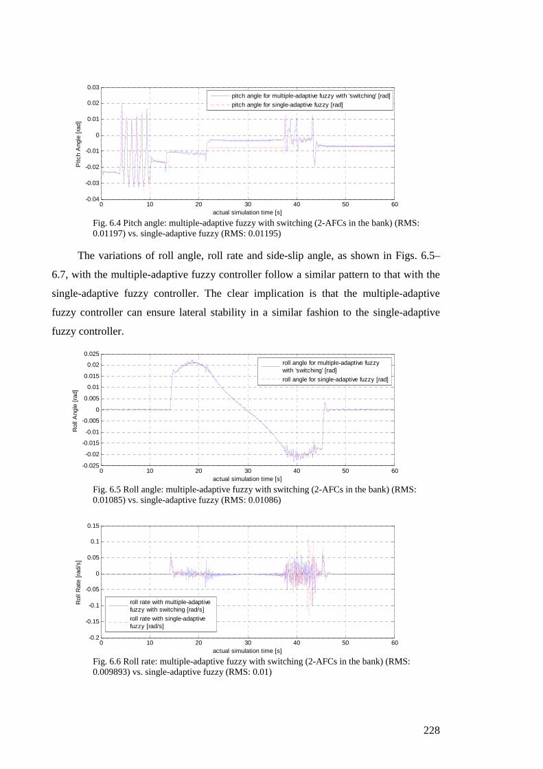
228
0 10 20 30 40 50 60-0.04
-0.03
-0.02
-0.01
0
0.01
0.02
0.03
actual simulation time [s]
Pitc
h A
ngle
[ra
d]
pitch angle for multiple-adaptive fuzzy with 'switching' [rad]
pitch angle for single-adaptive fuzzy [rad]
Fig. 6.4 Pitch angle: multiple-adaptive fuzzy with switching (2-AFCs in the bank) (RMS: 0.01197) vs. single-adaptive fuzzy (RMS: 0.01195)
The variations of roll angle, roll rate and side-slip angle, as shown in Figs. 6.5–
6.7, with the multiple-adaptive fuzzy controller follow a similar pattern to that with the
single-adaptive fuzzy controller. The clear implication is that the multiple-adaptive
fuzzy controller can ensure lateral stability in a similar fashion to the single-adaptive
fuzzy controller.
0 10 20 30 40 50 60-0.025
-0.02
-0.015
-0.01
-0.005
0
0.005
0.01
0.015
0.02
0.025
actual simulation time [s]
Rol
l Ang
le [
rad]
roll angle for multiple-adaptive fuzzy with 'switching' [rad]
roll angle for single-adaptive fuzzy [rad]
Fig. 6.5 Roll angle: multiple-adaptive fuzzy with switching (2-AFCs in the bank) (RMS: 0.01085) vs. single-adaptive fuzzy (RMS: 0.01086)
0 10 20 30 40 50 60-0.2
-0.15
-0.1
-0.05
0
0.05
0.1
0.15
actual simulation time [s]
Rol
l Rat
e [r
ad/s
]
roll rate with multiple-adaptive fuzzy with switching [rad/s]
roll rate with single-adaptive fuzzy [rad/s]
Fig. 6.6 Roll rate: multiple-adaptive fuzzy with switching (2-AFCs in the bank) (RMS: 0.009893) vs. single-adaptive fuzzy (RMS: 0.01)

229
0 10 20 30 40 50 60-0.015
-0.01
-0.005
0
0.005
0.01
0.015
0.02
actual simulation time [s]
Sid
e S
lip A
ngle
[ra
d]
side slip angle for multiple-adaptive fuzzy 'switching' [rad]
side slip angle for single-adaptive fuzzy [rad]
Fig. 6.7 Side-slip angle: multiple-adaptive fuzzy with switching (2-AFCs in the bank) (RMS: 0.07198) vs. single-adaptive fuzzy (RMS: 0.007206)
Since variations of lateral acceleration, as shown in Fig. 6.8, are well within the
limits of 4 [m/s2], it suggests that the multiple-adaptive fuzzy controller with switching
fulfils the design requirements of the passenger vehicles [178].
0 10 20 30 40 50 60-4
-3
-2
-1
0
1
2
3
actual simulation time [s]
Late
ral A
ccel
erat
ion
[m/s
2 ]
lateral acceleration with multiple-adaptive fuzzy with switching [m/s 2]
lateral acceleration with single-adaptive fuzzy [m/s 2]
Fig. 6.8 Lateral acceleration: multiple-adaptive fuzzy with switching (2-AFCs in the bank) (RMS: 1.264) vs. single-adaptive fuzzy (RMS: 1.264)
Overall, under normal cruising conditions, the multiple-adaptive fuzzy controller
with switching has ensured that it follows good tracking performance in lateral and
longitudinal aspects, in comparison to the single-adaptive fuzzy controller. In terms of
lateral stability, it can be said that the multiple-adaptive fuzzy controller with switching
performs as well as the single-adaptive fuzzy controller.
(b) External Disturbances: Multiple-Adaptive Fuzzy Control with Switching (2-AFCs)
In the following simulations, the developed multiple-adaptive fuzzy controller
with switching was tested against the single-adaptive fuzzy controller under a number
of external disturbances. These disturbances included addition of an un-symmetrical
load mass, presence of crosswind forces, and change of tyre-road friction.
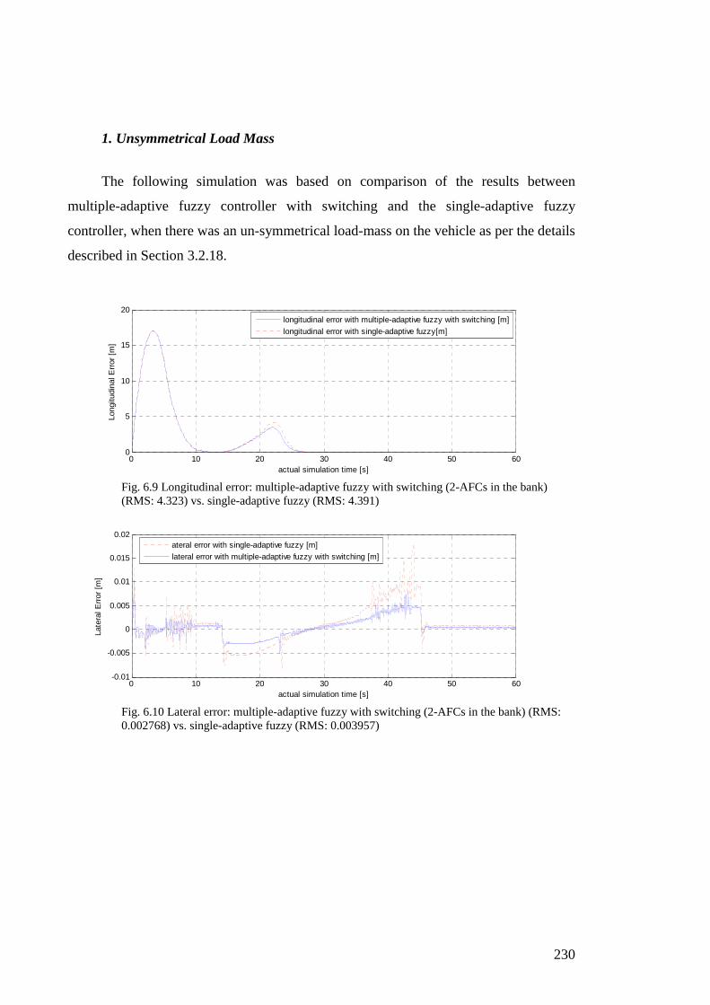
230
1. Unsymmetrical Load Mass
The following simulation was based on comparison of the results between
multiple-adaptive fuzzy controller with switching and the single-adaptive fuzzy
controller, when there was an un-symmetrical load-mass on the vehicle as per the details
described in Section 3.2.18.
0 10 20 30 40 50 600
5
10
15
20
actual simulation time [s]
Long
itudi
nal E
rror
[m
]
longitudinal error with multiple-adaptive fuzzy with switching [m]
longitudinal error with single-adaptive fuzzy[m]
Fig. 6.9 Longitudinal error: multiple-adaptive fuzzy with switching (2-AFCs in the bank) (RMS: 4.323) vs. single-adaptive fuzzy (RMS: 4.391)
0 10 20 30 40 50 60-0.01
-0.005
0
0.005
0.01
0.015
0.02
actual simulation time [s]
Late
ral E
rror
[m
]
ateral error with single-adaptive fuzzy [m]
lateral error with multiple-adaptive fuzzy with switching [m]
Fig. 6.10 Lateral error: multiple-adaptive fuzzy with switching (2-AFCs in the bank) (RMS: 0.002768) vs. single-adaptive fuzzy (RMS: 0.003957)

231
0 10 20 30 40 50 60-0.05
-0.04
-0.03
-0.02
-0.01
0
0.01
actual simulation time [s]
Pitc
h A
ngle
[ra
d]
pitch angle with multiple-adaptive fuzzy with switching [rad]
pitch angle with single-adaptive fuzzy [rad]
Fig. 6.11 Pitch angle: multiple-adaptive fuzzy with switching (2-AFCs in the bank) (RMS: 0.01972) vs. single-adaptive fuzzy (RMS: 0.01998)
0 10 20 30 40 50 60-0.04
-0.035
-0.03
-0.025
-0.02
-0.015
-0.01
-0.005
0
0.005
0.01
actual simulation time [s]
Rol
l Ang
le [
rad]
roll angle with multiple-adaptive fuzzy with switching [rad]
roll angle with single-adaptive fuzzy [rad]
Fig. 6.12 Roll angle: multiple-adaptive fuzzy with switching (2-AFCs in the bank) (RMS: 0.01766) vs. single-adaptive fuzzy (RMS: 0.01766)
0 10 20 30 40 50 60-0.1
-0.08
-0.06
-0.04
-0.02
0
0.02
0.04
0.06
0.08
0.1
actual simulation time [s]
Rol
l Rat
e [r
ad/s
]
roll rate with multiple-adaptive fuzzy with switching [rad/s]
roll rate with single-adaptive fuzzy [rad/s]
Fig. 6.13 Roll rate: multiple-adaptive fuzzy with switching (2-AFCs in the bank) (RMS: 0.01173) vs. single-adaptive fuzzy (RMS: 0.015)
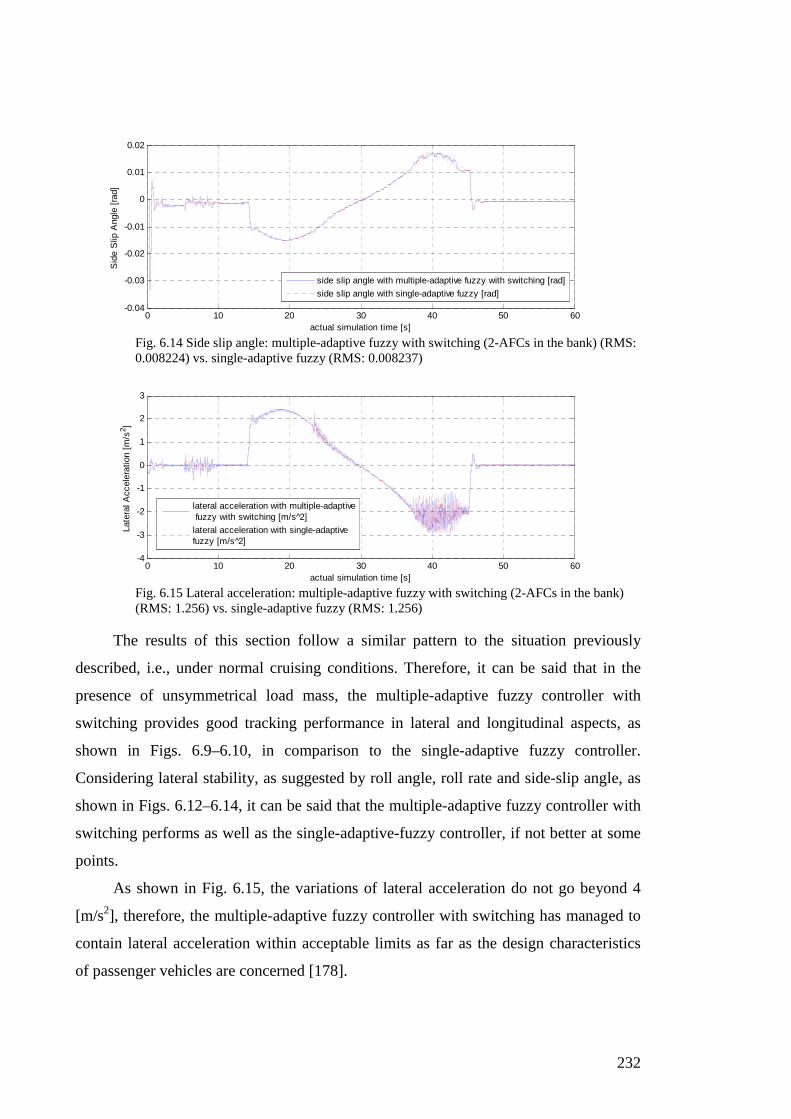
232
0 10 20 30 40 50 60-0.04
-0.03
-0.02
-0.01
0
0.01
0.02
actual simulation time [s]
Sid
e S
lip A
ngle
[ra
d]
side slip angle with multiple-adaptive fuzzy with switching [rad]
side slip angle with single-adaptive fuzzy [rad]
Fig. 6.14 Side slip angle: multiple-adaptive fuzzy with switching (2-AFCs in the bank) (RMS: 0.008224) vs. single-adaptive fuzzy (RMS: 0.008237)
0 10 20 30 40 50 60-4
-3
-2
-1
0
1
2
3
actual simulation time [s]
Late
ral A
ccel
erat
ion
[m/s
2 ]
lateral acceleration with multiple-adaptive fuzzy with switching [m/s 2]
lateral acceleration with single-adaptive fuzzy [m/s 2]
Fig. 6.15 Lateral acceleration: multiple-adaptive fuzzy with switching (2-AFCs in the bank) (RMS: 1.256) vs. single-adaptive fuzzy (RMS: 1.256)
The results of this section follow a similar pattern to the situation previously
described, i.e., under normal cruising conditions. Therefore, it can be said that in the
presence of unsymmetrical load mass, the multiple-adaptive fuzzy controller with
switching provides good tracking performance in lateral and longitudinal aspects, as
shown in Figs. 6.9–6.10, in comparison to the single-adaptive fuzzy controller.
Considering lateral stability, as suggested by roll angle, roll rate and side-slip angle, as
shown in Figs. 6.12–6.14, it can be said that the multiple-adaptive fuzzy controller with
switching performs as well as the single-adaptive-fuzzy controller, if not better at some
points.
As shown in Fig. 6.15, the variations of lateral acceleration do not go beyond 4
[m/s2], therefore, the multiple-adaptive fuzzy controller with switching has managed to
contain lateral acceleration within acceptable limits as far as the design characteristics
of passenger vehicles are concerned [178].

233
2. Crosswind Effects
The following simulation results were obtained when there was a presence of a
continuous crosswind with a speed of 50 [m/s] through the global y-direction. More
details of this arrangement are described in Section 3.2.18.
0 10 20 30 40 50 600
2
4
6
8
10
12
14
16
actual simulation time [s]
Long
itudi
nal E
rrio
r [m
]
longitudinal error with multiple-adaptive fuzzy with switching [m]
longitudinal error with single-adaptive fuzzy [m]
Fig. 6.16 Longitudinal error: multiple-adaptive fuzzy with switching (2-AFCs in the bank) (RMS: 3.744) vs. single-adaptive fuzzy (RMS: 3.742)
0 10 20 30 40 50 60-0.01
0
0.01
0.02
0.03
0.04
actual simulation time [s]
Late
ral E
rror
[m
]
lateral error with single-adaptive fuzzy[m]
lateral error with multiple-adaptive fuzzy with switching [m]
Fig. 6.17 Lateral error: multiple-adaptive fuzzy with switching (2-AFCs in the bank) (RMS: 0.002945) vs. single-adaptive fuzzy (RMS: 0.005914)
0 10 20 30 40 50 60-0.04
-0.03
-0.02
-0.01
0
0.01
0.02
actual simulation time [s]
Pitc
h A
ngle
[ra
d]
pitch angle with multiple-adaptive fuzzy with switching [rad]
pitch angle with single-adaptive fuzzy [rad]
Fig. 6.18 Pitch angle: multiple-adaptive fuzzy with switching (2-AFCs in the bank) (RMS: 0.01143) vs. single-adaptive fuzzy (RMS: 0.01142)
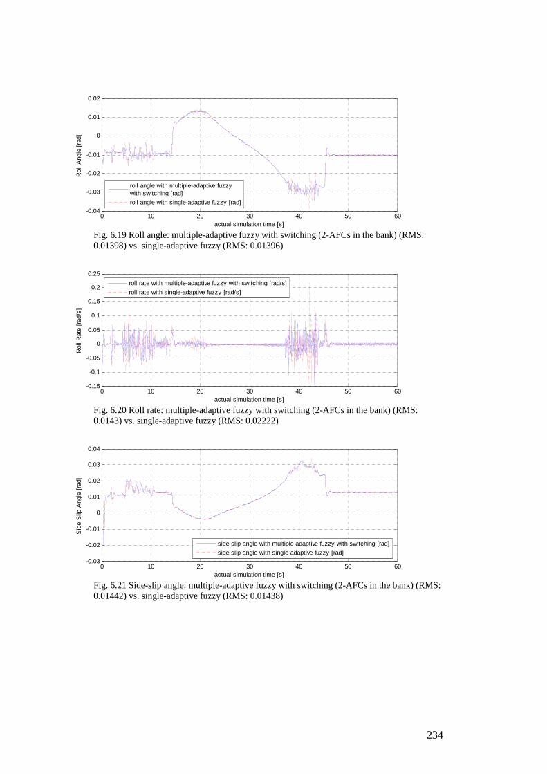
234
0 10 20 30 40 50 60-0.04
-0.03
-0.02
-0.01
0
0.01
0.02
actual simulation time [s]
Rol
l Ang
le [
rad]
roll angle with multiple-adaptive fuzzy with switching [rad]
roll angle with single-adaptive fuzzy [rad]
Fig. 6.19 Roll angle: multiple-adaptive fuzzy with switching (2-AFCs in the bank) (RMS: 0.01398) vs. single-adaptive fuzzy (RMS: 0.01396)
0 10 20 30 40 50 60-0.15
-0.1
-0.05
0
0.05
0.1
0.15
0.2
0.25
actual simulation time [s]
Rol
l Rat
e [r
ad/s
]
roll rate with multiple-adaptive fuzzy with switching [rad/s]
roll rate with single-adaptive fuzzy [rad/s]
Fig. 6.20 Roll rate: multiple-adaptive fuzzy with switching (2-AFCs in the bank) (RMS: 0.0143) vs. single-adaptive fuzzy (RMS: 0.02222)
0 10 20 30 40 50 60-0.03
-0.02
-0.01
0
0.01
0.02
0.03
0.04
actual simulation time [s]
Sid
e S
lip A
ngle
[ra
d]
side slip angle with multiple-adaptive fuzzy with switching [rad]
side slip angle with single-adaptive fuzzy [rad]
Fig. 6.21 Side-slip angle: multiple-adaptive fuzzy with switching (2-AFCs in the bank) (RMS: 0.01442) vs. single-adaptive fuzzy (RMS: 0.01438)

235
0 10 20 30 40 50 60
-4
-3
-2
-1
0
1
2
3
actual simulation time [s]
Late
ral A
ccel
erat
ion
[m/s
2 ]
lateral acceleration for multiple-adaptive fuzzy with switching [m/s 2]
lateral acceleration for single-adaptive fuzzy [m/s 2]
Fig. 6.22 Lateral acceleration: multiple-adaptive fuzzy with switching (2-AFCs in the bank) (RMS: 1.285) vs. single-adaptive fuzzy (RMS: 1.285)
The results of this section can be summarised as follows. It can be said that in the
presence of crosswind effects, the multiple-adaptive fuzzy controller with switching
provides good tracking performance in lateral and longitudinal aspects, as shown in
Figs. 6.16–6.17, in comparison to the single-adaptive fuzzy controller. It can be further
said that lateral tracking has been better while longitudinal tracking follows a similar
level to that of the single-adaptive fuzzy controller.
As suggested by roll angle, roll rate and side-slip angle, as shown in Figs. 6.19–
6.21, it can be said that multiple-adaptive fuzzy controller with switching has ensured a
good level of lateral stability that is on par with the single-adaptive fuzzy controller.
As shown in Fig. 6.22, the variations of lateral acceleration are well within 4
[m/s2]. Therefore, the multiple-adaptive fuzzy controller with switching has managed to
limit lateral acceleration to within specified design characteristics for passenger vehicles
[178].
3. Tyre-Road Friction Change
The following simulation results show the performance of the multiple-adaptive
fuzzy controller verses the single-adaptive fuzzy controller when there was a change of
tyre-road friction in the range 100-200 [m], on the highway.
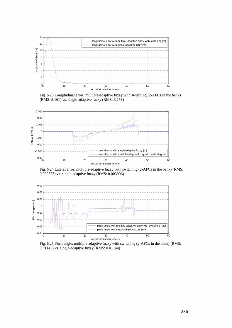
236
0 10 20 30 40 50 600
2
4
6
8
10
12
14
actual simulation time [s]
Long
itudi
nal E
rror
[m
]
longitudinal error with multiple-adaptive fuzzy with switching [m]
longitudinal error with single-adaptive fuzzy[m]
Fig. 6.23 Longitudinal error: multiple-adaptive fuzzy with switching (2-AFCs in the bank) (RMS: 3.161) vs. single-adaptive fuzzy (RMS: 3.158)
0 10 20 30 40 50 60-0.02
-0.015
-0.01
-0.005
0
0.005
0.01
0.015
actual simulation time [s]
Late
ral E
rror
[m
]
lateral error with single-adaptive fuzzy [m]
lateral error with multiple-adaptive fuzzy with switching [m]
Fig. 6.24 Lateral error: multiple-adaptive fuzzy with switching (2-AFCs in the bank) (RMS: 0.002573) vs. single-adaptive fuzzy (RMS: 0.003996)
0 10 20 30 40 50 60-0.04
-0.03
-0.02
-0.01
0
0.01
0.02
0.03
actual simulation time [s]
Pitc
h A
ngle
[ra
d]
pitch angle with multiple-adaptive fuzzy with switching [rad]
pitch angle with single-adaptive fuzzy [rad]
Fig. 6.25 Pitch angle: multiple-adaptive fuzzy with switching (2-AFCs in the bank) (RMS: 0.01143) vs. single-adaptive fuzzy (RMS: 0.01144)
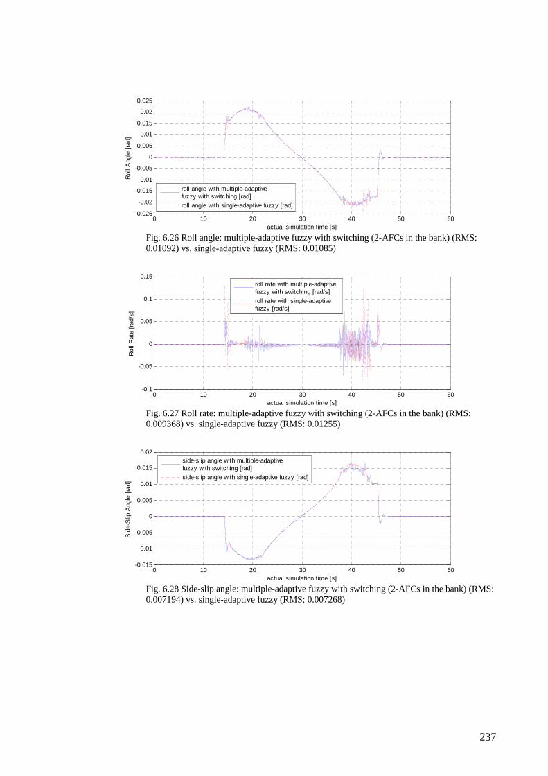
237
0 10 20 30 40 50 60-0.025
-0.02
-0.015
-0.01
-0.005
0
0.005
0.01
0.015
0.02
0.025
actual simulation time [s]
Rol
l Ang
le [
rad]
roll angle with multiple-adaptive fuzzy with switching [rad]
roll angle with single-adaptive fuzzy [rad]
Fig. 6.26 Roll angle: multiple-adaptive fuzzy with switching (2-AFCs in the bank) (RMS: 0.01092) vs. single-adaptive fuzzy (RMS: 0.01085)
0 10 20 30 40 50 60-0.1
-0.05
0
0.05
0.1
0.15
actual simulation time [s]
Rol
l Rat
e [r
ad/s
]
roll rate with multiple-adaptive fuzzy with switching [rad/s]
roll rate with single-adaptive fuzzy [rad/s]
Fig. 6.27 Roll rate: multiple-adaptive fuzzy with switching (2-AFCs in the bank) (RMS: 0.009368) vs. single-adaptive fuzzy (RMS: 0.01255)
0 10 20 30 40 50 60-0.015
-0.01
-0.005
0
0.005
0.01
0.015
0.02
actual simulation time [s]
Sid
e-S
lip A
ngle
[ra
d]
side-slip angle with multiple-adaptive fuzzy with switching [rad]
side-slip angle with single-adaptive fuzzy [rad]
Fig. 6.28 Side-slip angle: multiple-adaptive fuzzy with switching (2-AFCs in the bank) (RMS: 0.007194) vs. single-adaptive fuzzy (RMS: 0.007268)
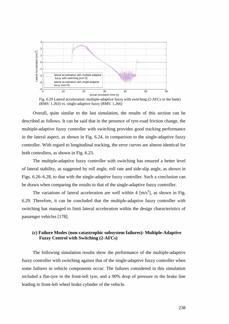
238
0 10 20 30 40 50 60-4
-3
-2
-1
0
1
2
3
actual simulation time [s]
Late
ral A
ccel
erat
ion
[m/s
2 ]
lateral acceleration with multiple-adaptive fuzzy with switching [m/s 2]
lateral acceleration with single-adaptive fuzzy [m/s 2]
Fig. 6.29 Lateral acceleration: multiple-adaptive fuzzy with switching (2-AFCs in the bank) (RMS: 1.263) vs. single-adaptive fuzzy (RMS: 1.266)
Overall, quite similar to the last simulation, the results of this section can be
described as follows. It can be said that in the presence of tyre-road friction change, the
multiple-adaptive fuzzy controller with switching provides good tracking performance
in the lateral aspect, as shown in Fig. 6.24, in comparison to the single-adaptive fuzzy
controller. With regard to longitudinal tracking, the error curves are almost identical for
both controllers, as shown in Fig. 6.23.
The multiple-adaptive fuzzy controller with switching has ensured a better level
of lateral stability, as suggested by roll angle, roll rate and side-slip angle, as shown in
Figs. 6.26–6.28, to that with the single-adaptive fuzzy controller. Such a conclusion can
be drawn when comparing the results to that of the single-adaptive fuzzy controller.
The variations of lateral acceleration are well within 4 [m/s2], as shown in Fig.
6.29. Therefore, it can be concluded that the multiple-adaptive fuzzy controller with
switching has managed to limit lateral acceleration within the design characteristics of
passenger vehicles [178].
(c) Failure Modes (non-catastrophic subsystem failures): Multiple-Adaptive Fuzzy Control with Switching (2-AFCs)
The following simulation results show the performance of the multiple-adaptive
fuzzy controller with switching against that of the single-adaptive fuzzy controller when
some failures in vehicle components occur. The failures considered in this simulation
included a flat-tyre in the front-left tyre, and a 90% drop of pressure in the brake line
leading to front-left wheel brake cylinder of the vehicle.

239
1. Flat-Tyre
0 10 20 30 40 50 600
10
20
30
40
50
60
actual simulation time [s]
Long
itudi
nal E
rror
[m
]
longitudinal error with multiple-adaptivefuzzy with switching [m]
longitudinal error with single-adaptive fuzzy [m]
Fig. 6.30 Longitudinal error: multiple-adaptive fuzzy with switching (2-AFCs in the bank) (RMS: 26.31) vs. single-adaptive fuzzy (RMS: 26.08)
0 10 20 30 40 50 60-0.02
0
0.02
0.04
0.06
0.08
0.1
0.12
0.14
actual simulation time [s]
Late
ral E
rror
[m
]
lateral error with single-adaptive fuzzy [m]
lateral error with multiple-adaptive fuzzy with switching [m]
Fig. 6.31 Lateral error: multiple-adaptive fuzzy with switching (2-AFCs in the bank) (RMS: 0.01017) vs. single-adaptive fuzzy (RMS: 0.02753)
0 10 20 30 40 50 60-0.04
-0.03
-0.02
-0.01
0
0.01
0.02
0.03
0.04
0.05
0.06
actual simulation time [s]
Pitc
h A
ngle
[ra
d]
pitch angle with multiple-adaptive fuzzy with switching [rad]
pitch angle with single-adaptive fuzzy [rad]
Fig. 6.32 Pitch angle: multiple-adaptive fuzzy with switching (2-AFCs in the bank) (RMS: 0.009741) vs. single-adaptive fuzzy (RMS: 0.01052)
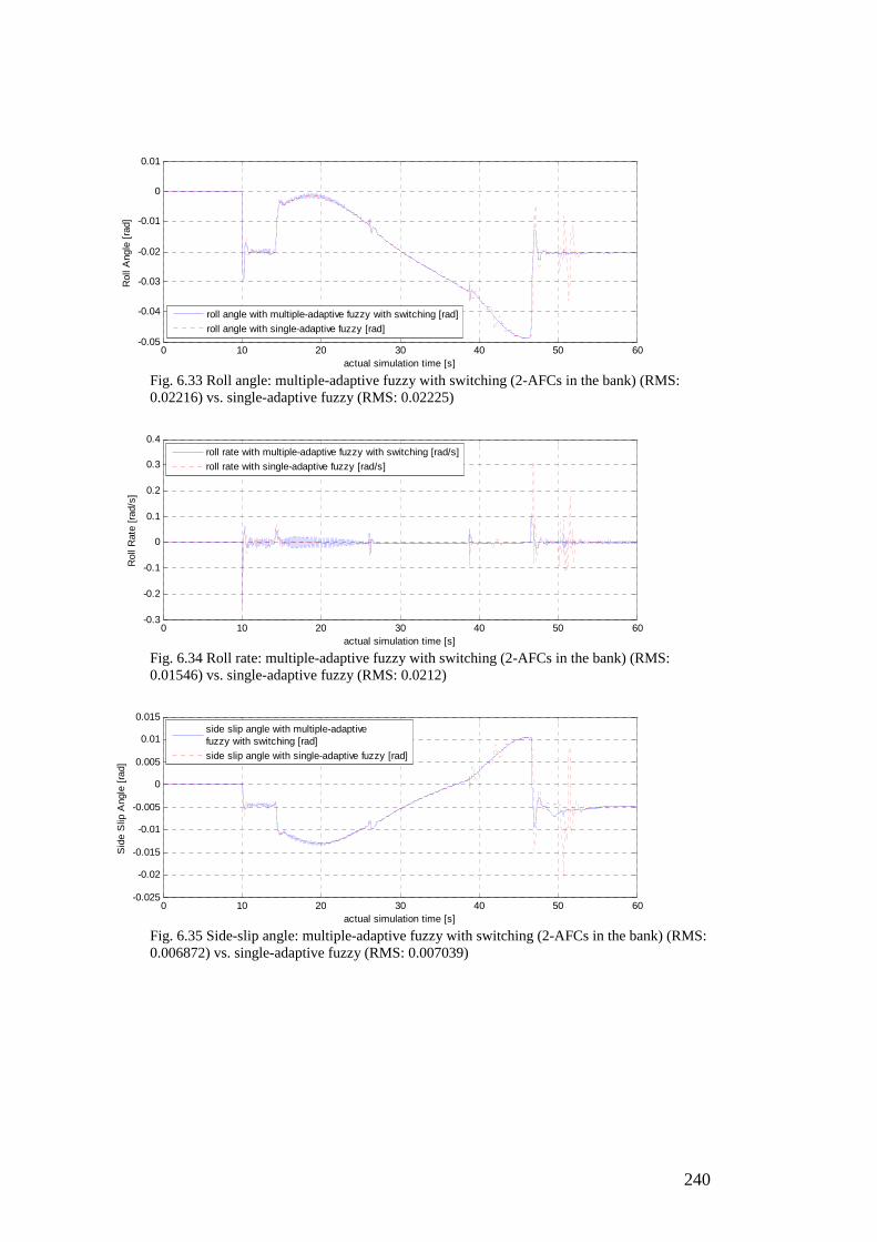
240
0 10 20 30 40 50 60-0.05
-0.04
-0.03
-0.02
-0.01
0
0.01
actual simulation time [s]
Rol
l Ang
le [
rad]
roll angle with multiple-adaptive fuzzy with switching [rad]
roll angle with single-adaptive fuzzy [rad]
Fig. 6.33 Roll angle: multiple-adaptive fuzzy with switching (2-AFCs in the bank) (RMS: 0.02216) vs. single-adaptive fuzzy (RMS: 0.02225)
0 10 20 30 40 50 60-0.3
-0.2
-0.1
0
0.1
0.2
0.3
0.4
actual simulation time [s]
Rol
l Rat
e [r
ad/s
]
roll rate with multiple-adaptive fuzzy with switching [rad/s]
roll rate with single-adaptive fuzzy [rad/s]
Fig. 6.34 Roll rate: multiple-adaptive fuzzy with switching (2-AFCs in the bank) (RMS: 0.01546) vs. single-adaptive fuzzy (RMS: 0.0212)
0 10 20 30 40 50 60-0.025
-0.02
-0.015
-0.01
-0.005
0
0.005
0.01
0.015
actual simulation time [s]
Sid
e S
lip A
ngle
[ra
d]
side slip angle with multiple-adaptive fuzzy with switching [rad]
side slip angle with single-adaptive fuzzy [rad]
Fig. 6.35 Side-slip angle: multiple-adaptive fuzzy with switching (2-AFCs in the bank) (RMS: 0.006872) vs. single-adaptive fuzzy (RMS: 0.007039)
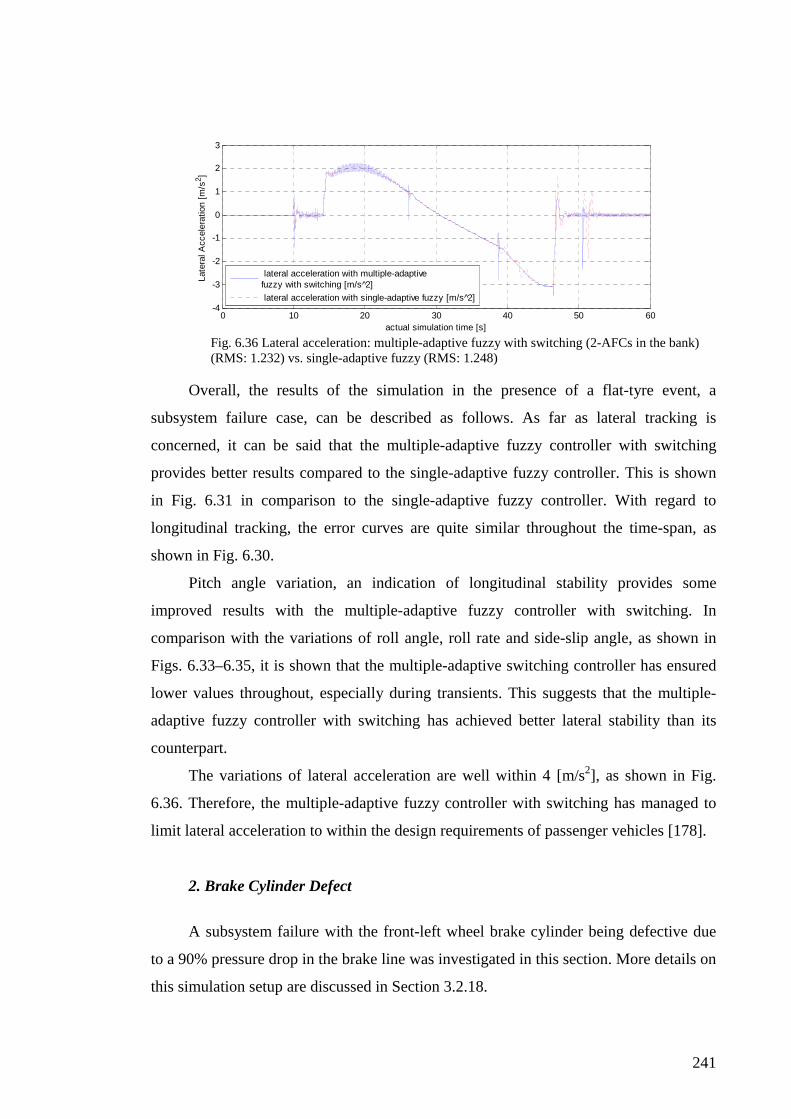
241
0 10 20 30 40 50 60-4
-3
-2
-1
0
1
2
3
actual simulation time [s]
Late
ral A
ccel
erat
ion
[m/s
2 ]
lateral acceleration with multiple-adaptive fuzzy with switching [m/s 2]
lateral acceleration with single-adaptive fuzzy [m/s 2]
Fig. 6.36 Lateral acceleration: multiple-adaptive fuzzy with switching (2-AFCs in the bank) (RMS: 1.232) vs. single-adaptive fuzzy (RMS: 1.248)
Overall, the results of the simulation in the presence of a flat-tyre event, a
subsystem failure case, can be described as follows. As far as lateral tracking is
concerned, it can be said that the multiple-adaptive fuzzy controller with switching
provides better results compared to the single-adaptive fuzzy controller. This is shown
in Fig. 6.31 in comparison to the single-adaptive fuzzy controller. With regard to
longitudinal tracking, the error curves are quite similar throughout the time-span, as
shown in Fig. 6.30.
Pitch angle variation, an indication of longitudinal stability provides some
improved results with the multiple-adaptive fuzzy controller with switching. In
comparison with the variations of roll angle, roll rate and side-slip angle, as shown in
Figs. 6.33–6.35, it is shown that the multiple-adaptive switching controller has ensured
lower values throughout, especially during transients. This suggests that the multiple-
adaptive fuzzy controller with switching has achieved better lateral stability than its
counterpart.
The variations of lateral acceleration are well within 4 [m/s2], as shown in Fig.
6.36. Therefore, the multiple-adaptive fuzzy controller with switching has managed to
limit lateral acceleration to within the design requirements of passenger vehicles [178].
2. Brake Cylinder Defect
A subsystem failure with the front-left wheel brake cylinder being defective due
to a 90% pressure drop in the brake line was investigated in this section. More details on
this simulation setup are discussed in Section 3.2.18.

242
0 10 20 30 40 50 600
2
4
6
8
10
12
14
actual simulation time [s]
Long
itudi
nal E
rror
[m
]
longitudinal error with multiple-adaptive fuzzy with switching [m]
longitudinal error with single-adaptive fuzzy [m]
Fig. 6.37 Longitudinal error: multiple-adaptive fuzzy with switching (2-AFCs in the bank) (RMS: 3.156) vs. single-adaptive fuzzy (RMS: 3.159)
0 10 20 30 40 50 60-0.1
0
0.1
0.2
0.3
0.4
actual simulation time [s]
Late
ral E
rror
[m
]
lateral error with multiple-adaptive fuzzy with switching [m]
lateral error with single-adaptive fuzzy [m]
Fig. 6.38 Lateral error: multiple-adaptive fuzzy with switching (2-AFCs in the bank) (RMS: 0.02007) vs. single-adaptive fuzzy (RMS: 0.03453)
0 10 20 30 40 50 60-0.04
-0.03
-0.02
-0.01
0
0.01
0.02
0.03
0.04
actual simulation time [s]
Pitc
h A
ngle
[ra
d]
pitch angle with multiple-adaptive fuzzy with switching [rad]
pitch angle with single-adaptive fuzzy [rad]
Fig. 6.39 Pitch angle: multiple-adaptive fuzzy with switching (2-AFCs in the bank) (RMS: 0.01483) vs. single-adaptive fuzzy (RMS: 0.01583)
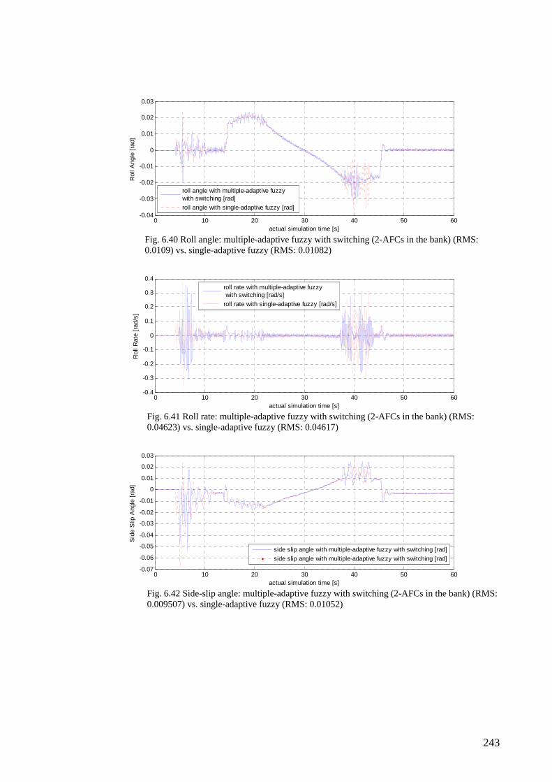
243
0 10 20 30 40 50 60-0.04
-0.03
-0.02
-0.01
0
0.01
0.02
0.03
actual simulation time [s]
Rol
l Ang
le [
rad]
roll angle with multiple-adaptive fuzzy with switching [rad]
roll angle with single-adaptive fuzzy [rad]
Fig. 6.40 Roll angle: multiple-adaptive fuzzy with switching (2-AFCs in the bank) (RMS: 0.0109) vs. single-adaptive fuzzy (RMS: 0.01082)
0 10 20 30 40 50 60-0.4
-0.3
-0.2
-0.1
0
0.1
0.2
0.3
0.4
actual simulation time [s]
Rol
l Rat
e [r
ad/s
]
roll rate with multiple-adaptive fuzzy with switching [rad/s]
roll rate with single-adaptive fuzzy [rad/s]
Fig. 6.41 Roll rate: multiple-adaptive fuzzy with switching (2-AFCs in the bank) (RMS: 0.04623) vs. single-adaptive fuzzy (RMS: 0.04617)
0 10 20 30 40 50 60-0.07
-0.06
-0.05
-0.04
-0.03
-0.02
-0.01
0
0.01
0.02
0.03
actual simulation time [s]
Sid
e S
lip A
ngle
[ra
d]
side slip angle with multiple-adaptive fuzzy with switching [rad]
side slip angle with multiple-adaptive fuzzy with switching [rad]
Fig. 6.42 Side-slip angle: multiple-adaptive fuzzy with switching (2-AFCs in the bank) (RMS: 0.009507) vs. single-adaptive fuzzy (RMS: 0.01052)

244
0 10 20 30 40 50 60-20
-15
-10
-5
0
5
10
actual simulation time [s]
Late
ral A
ccel
erat
ion
[m/s
2 ]
lateral acceleration with multiple-adaptive fuzzy with switching [m/s 2]
lateral acceleration with single-adaptive fuzzy [m/s 2]
Fig. 6.43 Lateral acceleration: multiple-adaptive fuzzy with switching (2-AFCs in the bank) (RMS: 1.314) vs. single-adaptive fuzzy (RMS: 1.334)
Overall, the results of the simulation of a defective front-left brake cylinder, a
subsystem failure case, are described as follows. It is seen that lateral tracking has been
better, as shown in Fig. 6.38, with regard to the multiple-adaptive fuzzy controller. As
far as longitudinal tracking is concerned, the performance of the two controllers is
similar, as shown in Fig. 6.37.
Pitch angle variation, an indication of longitudinal stability, shows some improved
response with the multiple-adaptive fuzzy controller with switching. Lateral stability
with the multiple-adaptive fuzzy controller has achieved an improved level in
comparison to that with the single-adaptive fuzzy controller. This conclusion is well
supported by the behaviour of roll angle, roll rate and side-slip angle, as shown in Figs.
6.40–6.42, where it is shown that the multiple-adaptive switching controller has ensured
lower values throughout, especially during transients.
The fact that variations of lateral acceleration are well within 4 [m/s2], as shown
in Fig. 6.43, suggests that the multiple-adaptive fuzzy controller with switching has
managed to limit lateral acceleration to within acceptable design requirements for
passenger vehicles [178].
Considering the overall performance of the multiple-adaptive fuzzy controller, the
level of lateral tracking has been better in comparison to that of the single-adaptive
fuzzy controller. The same cannot be said of longitudinal tracking, though. This is
because longitudinal curves, almost in every case, show they are almost identical for
both types of controllers. Another fact is that lateral stability has been maintained at a
good level by the multiple-adaptive fuzzy controller in comparison to that by the single-
adaptive fuzzy controller. It has also ensured that lateral acceleration is kept within

245
acceptable limits. Therefore, as a conclusion it can be said that the multiple-adaptive
fuzzy controller with switching has maintained good lateral tracking with ensured
lateral stability.
The summary of performance of the multiple-adaptive fuzzy controller with
switching with ‘two’ adaptive fuzzy controllers in the bank against that of the single-
adaptive fuzzy controller is provided in TABLE 6.1 below.
TABLE 6.1 Comparison of performance of fuzzy multiple-adaptive fuzzy controller (2 AFCs) against single-adaptive fuzzy controller
Performance
Simulation
long
itudi
nal e
rror
late
ral e
rror
pitc
h a
ngle
roll
ang
le
roll
rate
side
-slip
ang
le
late
ral a
cce
lera
tion
normal cruising similar significantly
improved similar similar similar similar similar
un-symmetrical loading
slightly improved
significantly improved
similar similar similar similar similar
crosswinds similar significantly improved
similar similar slightly
improved similar similar
tyre-road friction similar significantly improved
similar similar slightly
improved similar similar
flat- tyre similar significantly improved
slightly improved
slightly improved
slightly improved
slightly improved
similar
defective brake cylinder
similar improved similar similar similar slightly
improved significantly
improved
246
6.1.5 Simulation Studies, Results and Discussion for ‘Four’ Adaptive Fuzzy Controllers in the Bank (Multiple-Adaptive Fuzzy Controller with Switching)
In this simulation, the developed robust multiple-adaptive fuzzy controller with
switching, was included with ‘four’ adaptive fuzzy controllers in the bank for each
longitudinal and lateral controller.
(i) Simulation Setup
The simulation setup for this section was similar to the one described in Chapter 4
for the single-adaptive fuzzy controller system, except for facts otherwise stated in this
section. The simulation setup included veDYNA® setup, simulation profile details and
other settings.
In this simulation, multiple-adaptive fuzzy controller with switching was included
with four adaptive fuzzy controllers in the bank. Therefore, the adaptive gains were
taken as, 1 0.02xγ = , 2 0.03xγ = , 3 0.04xγ = , and 4 0.05xγ = for longitudinal case, and
1 0.005yγ = , 2 0.01yγ = , 3 0.02yγ = , and 4 0.03yγ = for lateral case, in the multiple-
adaptive fuzzy controller switching setup. This change in the range in adaptive gains is
due to the fact that lateral dynamics changes at a comparatively low rate than the
longitudinal.
(ii) Simulation Results and Discussion
In the following figures depicting simulation results, each performance parameter
of the multiple-adaptive fuzzy controller (solid blue line) is compared against that of the
single-adaptive fuzzy controller (dotted red line).
(a) Normal Cruising Conditions: Multiple-Adaptive Fuzzy Control with Switching (4-AFCs)
The following simulation results describe the performance of the developed
multiple-adaptive fuzzy controller against the results of the single-adaptive fuzzy
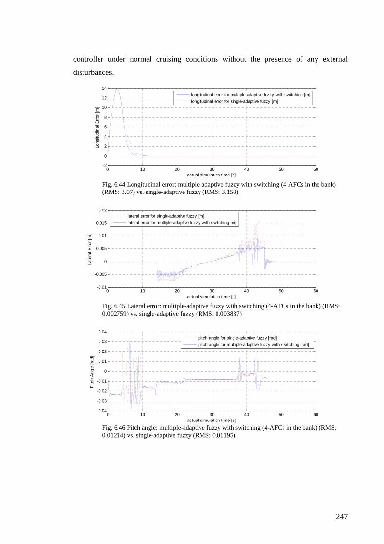
247
controller under normal cruising conditions without the presence of any external
disturbances.
0 10 20 30 40 50 60-2
0
2
4
6
8
10
12
14
actual simulation time [s]
Long
itudi
nal E
rror
[m
]
longitudinal error for multiple-adaptive fuzzy with switching [m]
longitudinal error for single-adaptive fuzzy [m]
Fig. 6.44 Longitudinal error: multiple-adaptive fuzzy with switching (4-AFCs in the bank) (RMS: 3.07) vs. single-adaptive fuzzy (RMS: 3.158)
0 10 20 30 40 50 60-0.01
-0.005
0
0.005
0.01
0.015
0.02
actual simulation time [s]
Late
ral E
rror
[m
]
lateral error for single-adaptive fuzzy [m]
lateral error for multiple-adaptive fuzzy with switching [m]
Fig. 6.45 Lateral error: multiple-adaptive fuzzy with switching (4-AFCs in the bank) (RMS: 0.002759) vs. single-adaptive fuzzy (RMS: 0.003837)
0 10 20 30 40 50 60-0.04
-0.03
-0.02
-0.01
0
0.01
0.02
0.03
0.04
actual simulation time [s]
Pitc
h A
ngle
[ra
d]
pitch angle for single-adaptive fuzzy [rad]
pitch angle for multiple-adaptive fuzzy with switching [rad]
Fig. 6.46 Pitch angle: multiple-adaptive fuzzy with switching (4-AFCs in the bank) (RMS: 0.01214) vs. single-adaptive fuzzy (RMS: 0.01195)

248
0 10 20 30 40 50 60-0.025
-0.02
-0.015
-0.01
-0.005
0
0.005
0.01
0.015
0.02
0.025
actual simulation time [s]
Rol
l Ang
le [
rad]
roll angle for multiple-adaptive fuzzy with switching [rad]
roll angle for single-adaptive fuzzy [rad]
Fig. 6.47 Roll angle: multiple-adaptive fuzzy with switching (4-AFCs in the bank) (RMS: 0.01085) vs. single-adaptive fuzzy (RMS: 0.01086)
0 10 20 30 40 50 60-0.08
-0.06
-0.04
-0.02
0
0.02
0.04
0.06
0.08
0.1
0.12
actual simulation time [s]
Rol
l Rat
e [r
ad/s
]
roll rate for single-adaptive fuzzy [rad/s]
roll rate for multiple-adaptive fuzzy with switching [rad/s]
Fig. 6.48 Roll rate: multiple-adaptive fuzzy with switching (4-AFCs in the bank) (RMS: 0.008191) vs. single-adaptive fuzzy (RMS: 0.01)
0 10 20 30 40 50 60-0.015
-0.01
-0.005
0
0.005
0.01
0.015
0.02
actual simulation time [s]
Sid
e-S
lip A
ngle
[ra
d]
side-slip angle for multiple-adaptive fuzzy with switching [rad]
side-slip angle for single-adaptive fuzzy [rad]
Fig. 6.49 Side-slip angle: multiple-adaptive fuzzy with switching (4-AFCs in the bank) (RMS: 0.007226) vs. single-adaptive fuzzy (RMS: 0.007206)
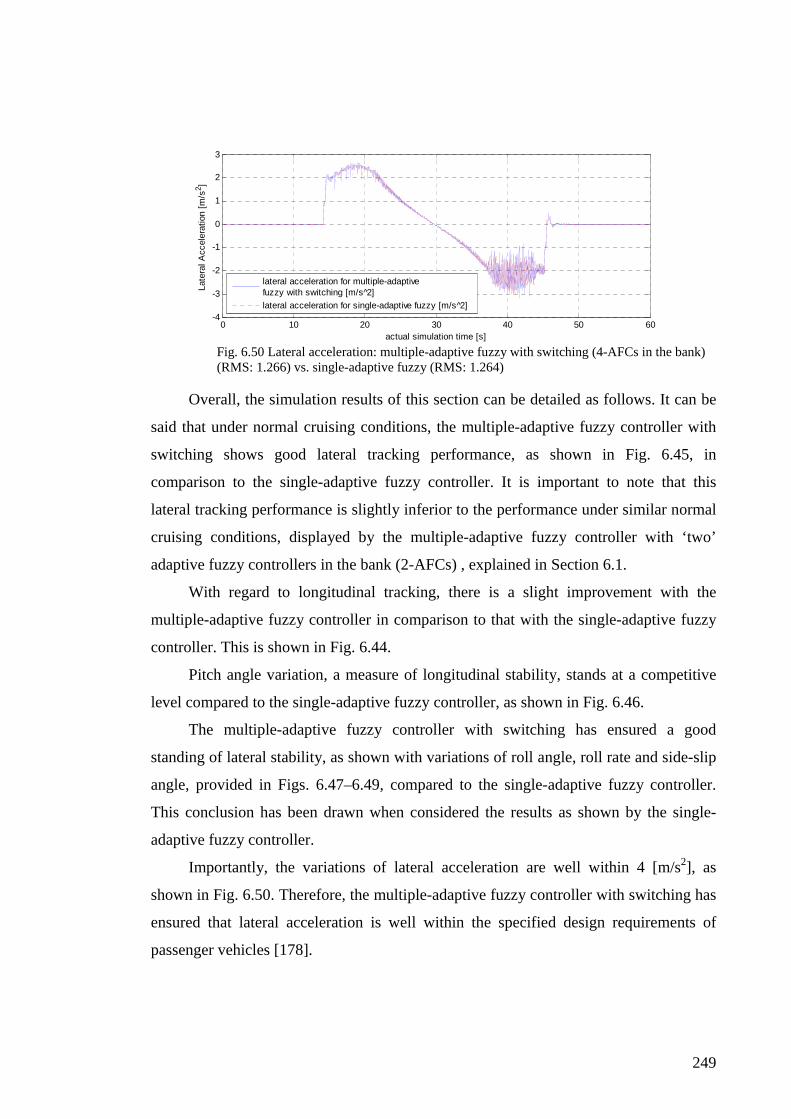
249
0 10 20 30 40 50 60-4
-3
-2
-1
0
1
2
3
actual simulation time [s]
Late
ral A
ccel
erat
ion
[m/s
2 ]
lateral acceleration for multiple-adaptive fuzzy with switching [m/s 2]
lateral acceleration for single-adaptive fuzzy [m/s 2]
Fig. 6.50 Lateral acceleration: multiple-adaptive fuzzy with switching (4-AFCs in the bank) (RMS: 1.266) vs. single-adaptive fuzzy (RMS: 1.264)
Overall, the simulation results of this section can be detailed as follows. It can be
said that under normal cruising conditions, the multiple-adaptive fuzzy controller with
switching shows good lateral tracking performance, as shown in Fig. 6.45, in
comparison to the single-adaptive fuzzy controller. It is important to note that this
lateral tracking performance is slightly inferior to the performance under similar normal
cruising conditions, displayed by the multiple-adaptive fuzzy controller with ‘two’
adaptive fuzzy controllers in the bank (2-AFCs) , explained in Section 6.1.
With regard to longitudinal tracking, there is a slight improvement with the
multiple-adaptive fuzzy controller in comparison to that with the single-adaptive fuzzy
controller. This is shown in Fig. 6.44.
Pitch angle variation, a measure of longitudinal stability, stands at a competitive
level compared to the single-adaptive fuzzy controller, as shown in Fig. 6.46.
The multiple-adaptive fuzzy controller with switching has ensured a good
standing of lateral stability, as shown with variations of roll angle, roll rate and side-slip
angle, provided in Figs. 6.47–6.49, compared to the single-adaptive fuzzy controller.
This conclusion has been drawn when considered the results as shown by the single-
adaptive fuzzy controller.
Importantly, the variations of lateral acceleration are well within 4 [m/s2], as
shown in Fig. 6.50. Therefore, the multiple-adaptive fuzzy controller with switching has
ensured that lateral acceleration is well within the specified design requirements of
passenger vehicles [178].

250
(b) External Disturbances: Multiple-Adaptive Fuzzy Control with Switching (4-AFCs)
In the following set of simulations, the developed multiple-adaptive fuzzy
controller with switching was tested against the single-adaptive fuzzy controller under a
number of external disturbances. These disturbances included addition of an
unsymmetrical load mass, presence of crosswind forces, and change of tyre-road
friction.
1. Unsymmetrical Load Mass
The following simulation was based on comparison of the results between the
multiple-adaptive fuzzy controller and the single-adaptive fuzzy controller, when there
was an un-symmetrical load-mass on the vehicle as per the details described in Section
3.2.18.
0 10 20 30 40 50 60-5
0
5
10
15
20
actual simulation time [s]
Long
itudi
nal E
rror
[m
]
longitudinal error for multiple-adaptive fuzzy with switching [m]
longitudinal error for single-adaptive fuzzy [m]
Fig. 6.51 Longitudinal error: multiple-adaptive fuzzy with switching (4-AFCs in the bank) (RMS: 3.587) vs. single-adaptive fuzzy (RMS: 4.391)
0 10 20 30 40 50 60-0.01
-0.005
0
0.005
0.01
0.015
0.02
actual simulation time [s]
Late
ral E
rror
[m
]
lateral error for multiple-adaptive fuzzy with switching [m]
lateral error for single-adaptive fuzzy [m]
Fig. 6.52 Lateral error: multiple-adaptive fuzzy with switching (4-AFCs in the bank) (RMS: 0.002848) vs. single-adaptive fuzzy (RMS: 0.003957)

251
0 10 20 30 40 50 60-0.05
-0.04
-0.03
-0.02
-0.01
0
0.01
actual simulation time [s]
Pitc
h A
ngle
[ra
d]
pitch angle for multiple-adaptive fuzzy with switching [rad]
pitch angle for single-adaptive fuzzy [rad]
Fig. 6.53 Pitch angle: multiple-adaptive fuzzy with switching (4-AFCs in the bank) (RMS: 0.01996) vs. single-adaptive fuzzy (RMS: 0.01998)
0 10 20 30 40 50 60-0.04
-0.035
-0.03
-0.025
-0.02
-0.015
-0.01
-0.005
0
0.005
0.01
actual simulation time [s]
Rol
l Ang
le [
rad]
roll angle for multiple-adaptive fuzzy with switching [rad]
roll angle for single-adaptive fuzzy [rad]
Fig. 6.54 Roll angle: multiple-adaptive fuzzy with switching (4-AFCs in the bank) (RMS: 0.01766) vs. single-adaptive fuzzy (RMS: 0.01766)
0 10 20 30 40 50 60-0.1
-0.05
0
0.05
0.1
0.15
actual simulation time [s]
Rol
l Rat
e [r
ad/s
]
roll rate for multiple-adaptive fuzzy with switching [rad/s]
roll rate for single-adaptive fuzzy [rad/s]
Fig. 6.55 Roll rate: multiple-adaptive fuzzy with switching (4-AFCs in the bank) (RMS: 0.01368) vs. single-adaptive fuzzy (RMS: 0.015)
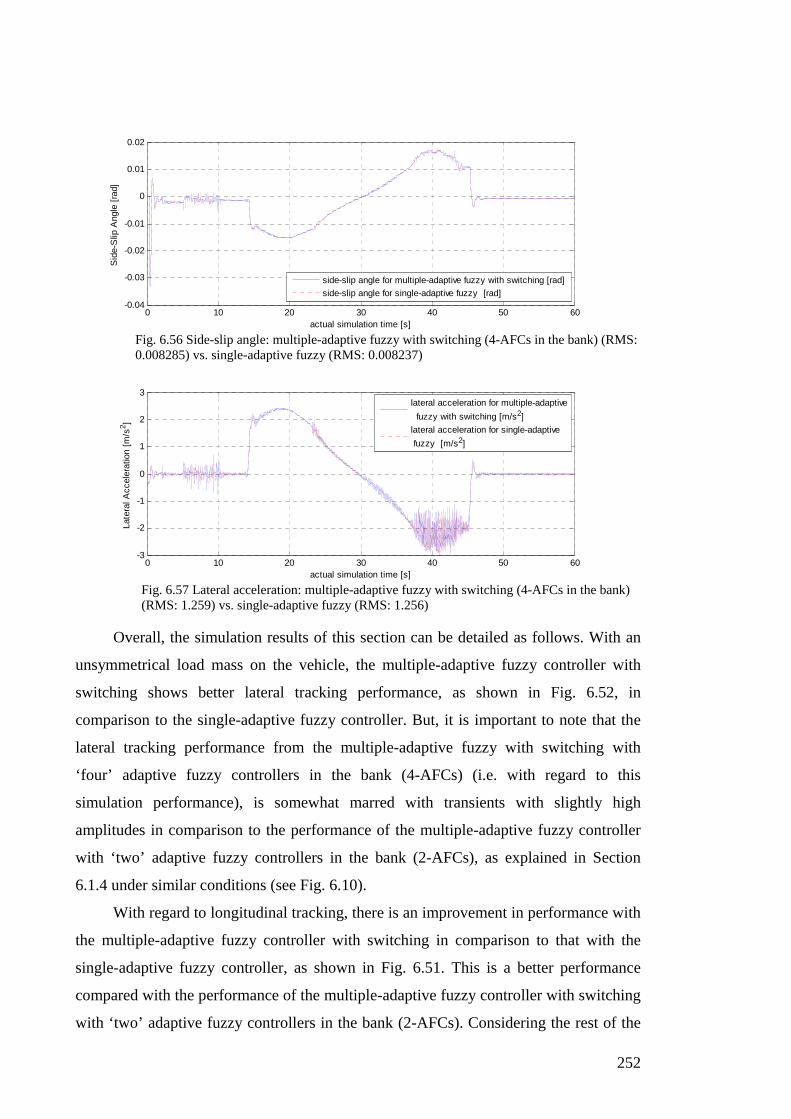
252
0 10 20 30 40 50 60-0.04
-0.03
-0.02
-0.01
0
0.01
0.02
actual simulation time [s]
Sid
e-S
lip A
ngle
[ra
d]
side-slip angle for multiple-adaptive fuzzy with switching [rad]
side-slip angle for single-adaptive fuzzy [rad]
Fig. 6.56 Side-slip angle: multiple-adaptive fuzzy with switching (4-AFCs in the bank) (RMS: 0.008285) vs. single-adaptive fuzzy (RMS: 0.008237)
0 10 20 30 40 50 60-3
-2
-1
0
1
2
3
actual simulation time [s]
Late
ral A
ccel
erat
ion
[m/s
2 ]
lateral acceleration for multiple-adaptive
fuzzy with switching [m/s2]
lateral acceleration for single-adaptive
fuzzy [m/s2]
Fig. 6.57 Lateral acceleration: multiple-adaptive fuzzy with switching (4-AFCs in the bank) (RMS: 1.259) vs. single-adaptive fuzzy (RMS: 1.256)
Overall, the simulation results of this section can be detailed as follows. With an
unsymmetrical load mass on the vehicle, the multiple-adaptive fuzzy controller with
switching shows better lateral tracking performance, as shown in Fig. 6.52, in
comparison to the single-adaptive fuzzy controller. But, it is important to note that the
lateral tracking performance from the multiple-adaptive fuzzy with switching with
‘four’ adaptive fuzzy controllers in the bank (4-AFCs) (i.e. with regard to this
simulation performance), is somewhat marred with transients with slightly high
amplitudes in comparison to the performance of the multiple-adaptive fuzzy controller
with ‘two’ adaptive fuzzy controllers in the bank (2-AFCs), as explained in Section
6.1.4 under similar conditions (see Fig. 6.10).
With regard to longitudinal tracking, there is an improvement in performance with
the multiple-adaptive fuzzy controller with switching in comparison to that with the
single-adaptive fuzzy controller, as shown in Fig. 6.51. This is a better performance
compared with the performance of the multiple-adaptive fuzzy controller with switching
with ‘two’ adaptive fuzzy controllers in the bank (2-AFCs). Considering the rest of the
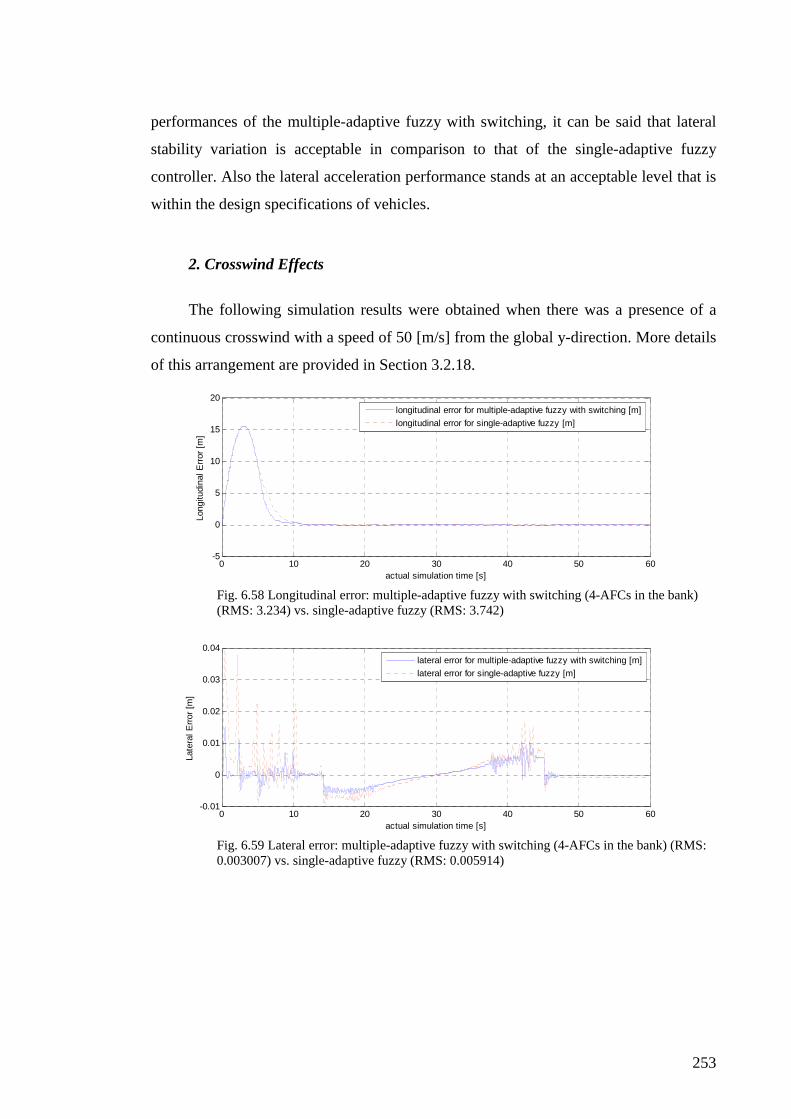
253
performances of the multiple-adaptive fuzzy with switching, it can be said that lateral
stability variation is acceptable in comparison to that of the single-adaptive fuzzy
controller. Also the lateral acceleration performance stands at an acceptable level that is
within the design specifications of vehicles.
2. Crosswind Effects
The following simulation results were obtained when there was a presence of a
continuous crosswind with a speed of 50 [m/s] from the global y-direction. More details
of this arrangement are provided in Section 3.2.18.
0 10 20 30 40 50 60-5
0
5
10
15
20
actual simulation time [s]
Long
itudi
nal E
rror
[m
]
longitudinal error for multiple-adaptive fuzzy with switching [m]
longitudinal error for single-adaptive fuzzy [m]
Fig. 6.58 Longitudinal error: multiple-adaptive fuzzy with switching (4-AFCs in the bank) (RMS: 3.234) vs. single-adaptive fuzzy (RMS: 3.742)
0 10 20 30 40 50 60-0.01
0
0.01
0.02
0.03
0.04
actual simulation time [s]
Late
ral E
rror
[m
]
lateral error for multiple-adaptive fuzzy with switching [m]
lateral error for single-adaptive fuzzy [m]
Fig. 6.59 Lateral error: multiple-adaptive fuzzy with switching (4-AFCs in the bank) (RMS: 0.003007) vs. single-adaptive fuzzy (RMS: 0.005914)

254
0 10 20 30 40 50 60-0.04
-0.03
-0.02
-0.01
0
0.01
0.02
0.03
actual simulation time [s]
Pitc
h A
ngle
[ra
d]
pitch angle for multiple-adaptive fuzzy with switching [rad]
pitch angle for single-adaptive fuzzy[rad]
Fig. 6.60 Pitch angle: multiple-adaptive fuzzy with switching (4-AFCs in the bank) (RMS: 0.011) vs. single-adaptive fuzzy (RMS: 0.01142)
0 10 20 30 40 50 60-0.04
-0.03
-0.02
-0.01
0
0.01
0.02
actual simulation time [s]
Rol
l Ang
le [
rad]
roll angle for multiple-adaptive fuzzy with switching [rad]
roll angle for single-adaptive fuzzy [rad]
Fig. 6.61 Roll angle: multiple-adaptive fuzzy with switching (4-AFCs in the bank) (RMS: 0.01402) vs. single-adaptive fuzzy (RMS: 0.01396)
0 10 20 30 40 50 60-0.15
-0.1
-0.05
0
0.05
0.1
0.15
0.2
0.25
actual simulation time [s]
Rol
l Rat
e [r
ad/s
]
roll rate for multiple-adaptive fuzzy with switching [rad/s]
roll rate for single-adaptive fuzzy [rad/s]
Fig. 6.62 Roll rate: multiple-adaptive fuzzy with switching (4-AFCs in the bank) (RMS: 0.01832) vs. single-adaptive fuzzy (RMS: 0.02222)

255
0 10 20 30 40 50 60-0.02
-0.01
0
0.01
0.02
0.03
0.04
0.05
actual simulation time [s]
Sid
e-S
lip A
ngle
[ra
d]
side-slip angle for multiple-adaptive fuzzy with switching [rad]
side-slip angle for single-adaptive fuzzy [rad]
Fig. 6.63 Side-slip angle: multiple-adaptive fuzzy with switching (4-AFCs in the bank) (RMS: 0.01486) vs. single-adaptive fuzzy (RMS: 0.01438)
0 10 20 30 40 50 60-4
-3
-2
-1
0
1
2
3
actual simulation time [s]
Late
ral A
ccel
erat
ion
[m/s
2 ]
lateral acceleration for multiple-adaptive fuzzy with switching [m/s 2]
lateral acceleration for single-adaptive fuzzy [m/s 2]
Fig. 6.64 Lateral acceleration: multiple-adaptive fuzzy with switching (4-AFCs in the bank) (RMS: 1.289) vs. single-adaptive fuzzy (RMS: 1.285)
Overall, the simulation results of this section can be described as follows. With
crosswind effects being present throughout, the multiple-adaptive fuzzy controller with
switching performed better in lateral tracking, as shown in Fig. 6.59, in comparison to
the single-adaptive fuzzy controller.
With regard to longitudinal tracking, there is an improvement in performance with
the multiple-adaptive fuzzy controller with switching in comparison to that with the
single-adaptive fuzzy controller, as shown in Fig. 6.56. This is a better performance
compared with the performance of the multiple-adaptive fuzzy controller with switching
with ‘two’ adaptive fuzzy controllers in the bank (2-AFCs).
Considering the rest of the performances of the multiple-adaptive fuzzy with
switching, it can be repeated as follows as provided in the last description. The lateral
stability variation is acceptable in comparison to that of the single-adaptive fuzzy
controller. Also the lateral acceleration performance stands at an acceptable level that is
within the design specifications of vehicles.
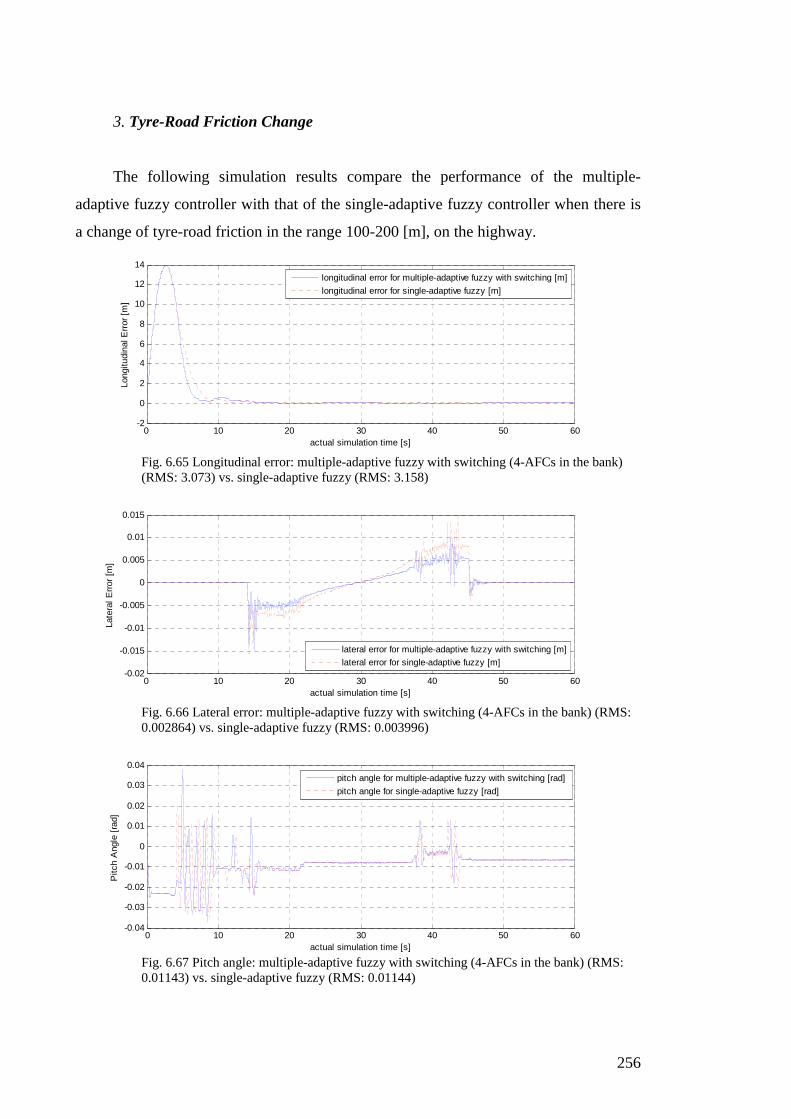
256
3. Tyre-Road Friction Change
The following simulation results compare the performance of the multiple-
adaptive fuzzy controller with that of the single-adaptive fuzzy controller when there is
a change of tyre-road friction in the range 100-200 [m], on the highway.
0 10 20 30 40 50 60-2
0
2
4
6
8
10
12
14
actual simulation time [s]
Long
itudi
nal E
rror
[m
]
longitudinal error for multiple-adaptive fuzzy with switching [m]
longitudinal error for single-adaptive fuzzy [m]
Fig. 6.65 Longitudinal error: multiple-adaptive fuzzy with switching (4-AFCs in the bank) (RMS: 3.073) vs. single-adaptive fuzzy (RMS: 3.158)
0 10 20 30 40 50 60-0.02
-0.015
-0.01
-0.005
0
0.005
0.01
0.015
actual simulation time [s]
Late
ral E
rror
[m
]
lateral error for multiple-adaptive fuzzy with switching [m]
lateral error for single-adaptive fuzzy [m]
Fig. 6.66 Lateral error: multiple-adaptive fuzzy with switching (4-AFCs in the bank) (RMS: 0.002864) vs. single-adaptive fuzzy (RMS: 0.003996)
0 10 20 30 40 50 60-0.04
-0.03
-0.02
-0.01
0
0.01
0.02
0.03
0.04
actual simulation time [s]
Pitc
h A
ngle
[ra
d]
pitch angle for multiple-adaptive fuzzy with switching [rad]
pitch angle for single-adaptive fuzzy [rad]
Fig. 6.67 Pitch angle: multiple-adaptive fuzzy with switching (4-AFCs in the bank) (RMS: 0.01143) vs. single-adaptive fuzzy (RMS: 0.01144)

257
0 10 20 30 40 50 60-0.03
-0.02
-0.01
0
0.01
0.02
0.03
actual simulation time [s]
Rol
l Ang
le [
rad]
roll angle for multiple-adaptive fuzzy with switching [rad]
roll angle for single-adaptive fuzzy [rad]
Fig. 6.68 Roll angle: multiple-adaptive fuzzy with switching (4-AFCs in the bank) (RMS: 0.01087) vs. single-adaptive fuzzy (RMS: 0.01085)
0 10 20 30 40 50 60-0.2
-0.15
-0.1
-0.05
0
0.05
0.1
0.15
actual simulation time [s]
Rol
l Rat
e [r
ad/s
]
roll rate for multiple-adaptive fuzzy with switching [rad/s]
roll rate for single-adaptive fuzzy [rad/s]
Fig. 6.69 Roll rate: multiple-adaptive fuzzy with switching (4-AFCs in the bank) (RMS: 0.01416) vs. single-adaptive fuzzy (RMS: 0.01255)
0 10 20 30 40 50 60-0.015
-0.01
-0.005
0
0.005
0.01
0.015
0.02
actual simulation time [s]
Sid
e-S
lip A
ngle
[ra
d]
side-slip angle for multiple-adaptive fuzzy with switching [rad]
side-slip angle for single-adaptive fuzzy [rad]
Fig. 6.70 Side-slip angle: multiple-adaptive fuzzy with switching (4-AFCs in the bank) (RMS: 0.007222) vs. single-adaptive fuzzy (RMS: 0.007268)

258
0 10 20 30 40 50 60-4
-3
-2
-1
0
1
2
3
actual simulation time [s]
Late
ral A
ccel
erat
ion
[m/s
2 ]
lateral acceleration for multiple-adaptive fuzzy with switching [m/s 2]
lateral acceleration for single-adaptive fuzzy [m/s 2]
Fig. 6.71 Lateral acceleration: multiple-adaptive fuzzy with switching (4-AFCs in the bank) (RMS: 1.265) vs. single-adaptive fuzzy (RMS: 1.266)
Overall, the simulation results of this section can be elaborated as follows. With a
tyre-road friction change, the multiple-adaptive fuzzy controller with switching shows
better lateral tracking performance, as shown in Fig. 6.66, in comparison to the single-
adaptive fuzzy controller. As far as lateral tracking performance of the multiple-
adaptive fuzzy with switching (4-AFCs) is concerned, it can be considered as somewhat
deteriorated with chattering in comparison to the performance of the multiple-adaptive
fuzzy with switching (2-AFCs), under similar conditions as described in Section 6.1.4
(see Fig. 6.24).
Again, longitudinal tracking performance with the multiple-adaptive fuzzy
controller with switching is better compared to that with the single-adaptive fuzzy
controller.
According to the collective performance in the areas of roll angle, roll-rate and
side-slip angle, lateral stability variation appears acceptable with the multiple-adaptive
fuzzy controller with switching. As far as lateral acceleration is concerned, the multiple-
adaptive fuzzy controller with switching can be accepted as performing within the
design specifications of passenger vehicles.
(c) Failure Modes: Multiple-Adaptive Fuzzy Control with Switching (4-AFCs)
The following simulation results show the performance of the multiple-adaptive
fuzzy with switching controller against the single-adaptive fuzzy controller when some
failures occur in the vehicle components. The failures considered in this simulation
included a flat-tyre in the front-left tyre, and a 90% drop of pressure in the brake line of
the front-left wheel cylinder of the vehicle.

259
1. Flat-Tyre
The following simulation results were obtained when an event of front-left tyre
becoming flat occurred at 10[s] after starting the simulation. The details of the
simulation arrangement are explained in Section 3.2.18.
0 10 20 30 40 50 60-10
0
10
20
30
40
50
60
actual simulation time [s]
Long
itudi
nal E
rror
[m
]
longitudinal error for multiple-adaptivefuzzy with switching [m]
longitudinal error for single-adaptive fuzzy [m]
Fig. 6.72 Longitudinal error: multiple-adaptive fuzzy with switching (4-AFCs in the bank) (RMS: 24.76) vs. single-adaptive fuzzy (RMS: 26.08)
0 10 20 30 40 50 60-0.05
0
0.05
0.1
0.15
actual simulation time [s]
Late
ral E
rror
[m
]
longitudinal error for multiple-adaptive fuzzy with switching [m]
longitudinal error for single-adaptive fuzzy [m]
Fig. 6.73 Lateral error: multiple-adaptive fuzzy with switching (4-AFCs in the bank) (RMS: 0.01137) vs. single-adaptive fuzzy (RMS: 0.02753)
0 10 20 30 40 50 60-0.04
-0.03
-0.02
-0.01
0
0.01
0.02
0.03
0.04
0.05
0.06
actual simulation time [s]
Pitc
h A
ngle
[ra
d]
pitch angle for multiple-adaptive fuzzy with switching [rad]
pitch angle for single-adaptive fuzzy[rad]
Fig. 6.74 Pitch angle: multiple-adaptive fuzzy with switching (4-AFCs in the bank) (RMS: 0.01078) vs. single-adaptive fuzzy (RMS: 0.01052)

260
0 10 20 30 40 50 60-0.05
-0.04
-0.03
-0.02
-0.01
0
0.01
actual simulation time [s]
Rol
l Ang
le [
rad]
roll angle for multiple-adaptive fuzzy with switching [rad]
roll angle for single-adaptive fuzzy [rad]
Fig. 6.75 Roll angle: multiple-adaptive fuzzy with switching (4-AFCs in the bank) (RMS: 0.02222) vs. single-adaptive fuzzy (RMS: 0.02225)
0 10 20 30 40 50 60-0.4
-0.3
-0.2
-0.1
0
0.1
0.2
0.3
0.4
0.5
actual simulation time [s]
Rol
l Rat
e [r
ad/s
]
roll rate for multiple-adaptive fuzzy with switching [rad/s]
roll rate for single-adaptive fuzzy [rad/s]
Fig. 6.76 Roll rate: multiple-adaptive fuzzy with switching (4-AFCs in the bank) (RMS: 0.03229) vs. single-adaptive fuzzy (RMS: 0.0212)
0 10 20 30 40 50 60-0.025
-0.02
-0.015
-0.01
-0.005
0
0.005
0.01
0.015
actual simulation time [s]
Sid
e-S
lip A
ngle
[ra
d]
side-slip angle for multiple-adaptive fuzzy with switching [rad]
side-slip angle for single-adaptive fuzzy [rad]
Fig. 6.77 Side-slip angle: multiple-adaptive fuzzy with switching (4-AFCs in the bank) (RMS: 0.007065) vs. single-adaptive fuzzy (RMS: 0.007039)

261
0 10 20 30 40 50 60-4
-3
-2
-1
0
1
2
3
actual simulation time [s]
Late
ral A
ccel
erat
ion
[m/s
2 ]
lateral acceleration for multiple-adaptive fuzzy with switching [m/s 2]
lateral acceleration for single-adaptive fuzzy [m/s 2]
Fig. 6.78 Lateral acceleration: multiple-adaptive fuzzy with switching (4-AFCs in the bank) (RMS: 1.254) vs. single-adaptive fuzzy (RMS: 1.248)
Overall, the simulation results of this section can be detailed as follows. With the
case of flat-tyre, the multiple-adaptive fuzzy controller with switching shows better
lateral tracking performance, as shown in Fig. 6.73, in comparison to the single-
adaptive fuzzy controller. The lateral tracking performance of the multiple-adaptive
fuzzy with switching, i.e., with 4-AFCs, becomes slightly worse around 50 –53 [s] on
the time-scale, and the effect can be seen on most parameters affected by transverse
motion of the vehicle. Such a deviation is clearly on the negative side of performance in
comparison to that of the multiple-adaptive fuzzy controller with ‘two’ adaptive fuzzy
controllers in the bank (2-AFCs) described in Section 6.1 (see Fig. 6.31).
With regard to longitudinal tracking, it provides some improved results with the
multiple-adaptive fuzzy controller in comparison to the single-adaptive fuzzy controller,
as shown in Fig. 6.72.
Pitch angle is at an improved level compared to the single-adaptive fuzzy
controller, as shown in Fig. 6.74.
Lateral stability variation also appears acceptable with the multiple-adaptive fuzzy
controller with switching. Conclusions on lateral stability have been inferred from the
variations of roll angle, roll rate and side-slip angle as illustrated in Figs. 6.75–6.77.
Such a conclusion can be drawn after comparing the results with that of the single-
adaptive fuzzy controller.
Once again, the variation of lateral acceleration falls within 4 [m/s2], as shown in
Fig. 6.78. Therefore, the multiple-adaptive fuzzy controller ensures that lateral
acceleration is maintained at an acceptable level as required by the design specifications
of passenger vehicles [178].

262
2. Brake Cylinder Defect
The investigation of a subsystem failure of front-left wheel-brake cylinder being
defective due to a 90% pressure drop in the brake line is studied in this section. More
details on this simulation setup are discussed in Section 3.2.18.
0 10 20 30 40 50 60-2
0
2
4
6
8
10
12
14
actual simulation time [s]
Long
itudi
nal E
rror
[m
]
longitudinal error for multiple-adaptive fuzzy with switching [m]
longitudinal error for single-adaptive fuzzy [m]
Fig. 6.79 Longitudinal error: multiple-adaptive fuzzy with switching (4-AFCs in the bank) (RMS: 3.062) vs. single-adaptive fuzzy (RMS: 3.159)
0 10 20 30 40 50 60-0.1
0
0.1
0.2
0.3
0.4
actual simulation time [s]
Late
ral E
rror
[m
]
lateral error for single-adaptive fuzzy [m]
lateral error for multiple-adaptive fuzzy with switching [m]
Fig. 6.80 Lateral error: multiple-adaptive fuzzy with switching (4-AFCs in the bank) (RMS: 0.02255) vs. single-adaptive fuzzy (RMS: 0.03453)
0 10 20 30 40 50 60-0.05
-0.04
-0.03
-0.02
-0.01
0
0.01
0.02
0.03
0.04
actual simulation time [s]
Pitc
h A
ngle
[ra
d]
pitch angle for multiple-adaptive fuzzy with switching [rad]
pitch angle for single-adaptive fuzzy [rad]
Fig. 6.81 Pitch angle: multiple-adaptive fuzzy with switching (4-AFCs in the bank) (RMS: 0.01479) vs. single-adaptive fuzzy (RMS: 0.01583)
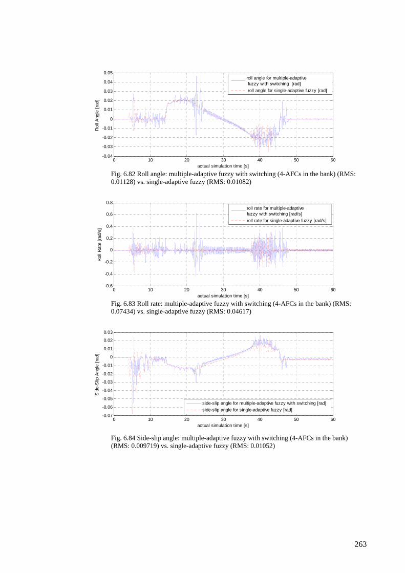
263
0 10 20 30 40 50 60-0.04
-0.03
-0.02
-0.01
0
0.01
0.02
0.03
0.04
0.05
actual simulation time [s]
Rol
l Ang
le [
rad]
roll angle for multiple-adaptive fuzzy with switching [rad]
roll angle for single-adaptive fuzzy [rad]
Fig. 6.82 Roll angle: multiple-adaptive fuzzy with switching (4-AFCs in the bank) (RMS: 0.01128) vs. single-adaptive fuzzy (RMS: 0.01082)
0 10 20 30 40 50 60-0.6
-0.4
-0.2
0
0.2
0.4
0.6
0.8
actual simulation time [s]
Rol
l Rat
e [r
ad/s
]
roll rate for multiple-adaptive fuzzy with switching [rad/s]
roll rate for single-adaptive fuzzy [rad/s]
Fig. 6.83 Roll rate: multiple-adaptive fuzzy with switching (4-AFCs in the bank) (RMS: 0.07434) vs. single-adaptive fuzzy (RMS: 0.04617)
0 10 20 30 40 50 60-0.07
-0.06
-0.05
-0.04
-0.03
-0.02
-0.01
0
0.01
0.02
0.03
actual simulation time [s]
Sid
e-S
lip A
ngle
[ra
d]
side-slip angle for multiple-adaptive fuzzy with switching [rad]
side-slip angle for single-adaptive fuzzy [rad]
Fig. 6.84 Side-slip angle: multiple-adaptive fuzzy with switching (4-AFCs in the bank) (RMS: 0.009719) vs. single-adaptive fuzzy (RMS: 0.01052)

264
0 10 20 30 40 50 60-20
-15
-10
-5
0
5
10
actual simulation time [s]
Late
ral A
ccel
erat
ion
[m/s
2 ]
lateral acceleration for multiple-adaptive fuzzy with switching [m/s 2]
lateral acceleration for single-adaptive fuzzy [m/s 2]
Fig. 6.85 Lateral acceleration: multiple-adaptive fuzzy with switching (4-AFCs in the bank) (RMS: 1.384) vs. single-adaptive fuzzy (RMS: 1.334)
Overall, the simulation results of this section can be discussed as follows. With a
brake cylinder defect, the multiple-adaptive fuzzy controller with switching shows some
improved lateral tracking performance, as shown in Fig. 6.80, in comparison to the
single-adaptive fuzzy controller.
With regard to longitudinal tracking, there is some improvement with the
multiple-adaptive fuzzy controller in comparison to the single-adaptive fuzzy controller,
as shown in Fig. 6.79.
The variation of pitch angle again stands at an acceptable level when compared to
the single-adaptive fuzzy controller, as shown in Fig. 6.81.
Once again, lateral stability variation appears acceptable with the multiple-
adaptive fuzzy controller with switching. This result is inferred from the variations of
roll angle, roll rate and side-slip angle shown in Figs. 6.82–6.84. Such a conclusion can
be drawn when the results are compared to that shown by the single-adaptive fuzzy
controller.
As far as lateral acceleration is concerned, it stands close to 4 [m/s2] with the
multiple-adaptive fuzzy controller with switching as shown in Fig. 6.85. This can be
compared against the performances of the single-adaptive fuzzy controller, as shown in
the same figure. Therefore, it can be said that the multiple-adaptive fuzzy controller
performs exceptionally well in relation to the design requirements of passenger vehicles
[178].
Considering the overall performance of the multiple-adaptive fuzzy controller
with switching, the level of lateral tracking has been good in comparison to that of the
single-adaptive fuzzy controller. But, it has to be mentioned that the level of

265
achievement with lateral tracking is somewhat lower in comparison to the results in
Section 6.1.4 for the multiple-adaptive fuzzy controller with switching having ‘two’
adaptive fuzzy controllers in the bank (2-AFCs).
In contrast to the results obtained in Section 6.1, there have been some improved
results with longitudinal tracking with regard to the multiple-adaptive fuzzy controller
with switching (4-AFCs), though.
Another feature is that lateral stability has been maintained at an acceptable level
by the multiple-adaptive fuzzy controller. According to the design requirements, the
multiple-adaptive fuzzy controller with switching has ensured that lateral acceleration is
kept within acceptable limits.
The summary of performances of the multiple-adaptive fuzzy controller with
switching with ‘four’ adaptive fuzzy controllers in the bank against that of single-
adaptive fuzzy controller is provided in TABLE 6.2 below.
TABLE 6.2 Comparison of performance of fuzzy multiple-adaptive fuzzy controller (4 AFCs)
against single-adaptive fuzzy controller
Performance
Simulation
long
itudi
nal e
rror
late
ral e
rror
pitc
h a
ngle
roll
ang
le
roll
rate
side
-slip
ang
le
late
ral a
cce
lera
tion
normal cruising slightly
improved improved similar similar
slightly improved
similar similar
un-symmetrical loading
slightly improved
improved similar similar slightly
improved similar similar
crosswinds slightly
improved significantly
improved similar similar
slightly improved
similar similar
tyre-road friction
slightly improved
improved similar similar similar similar similar
flat- tyre improved improved similar similar slightly
deteriorated similar similar
defective brake cylinder
improved improved similar slightly
deteriorated slightly
deteriorated slightly
improved similar
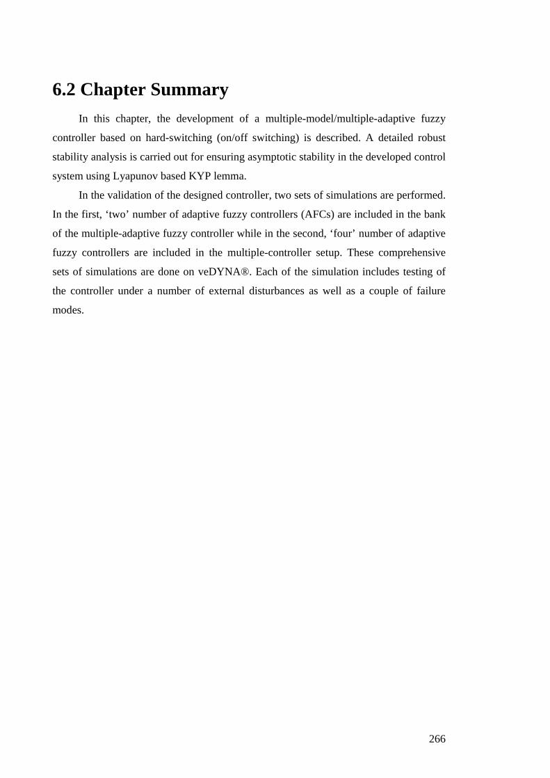
266
6.2 Chapter Summary
In this chapter, the development of a multiple-model/multiple-adaptive fuzzy
controller based on hard-switching (on/off switching) is described. A detailed robust
stability analysis is carried out for ensuring asymptotic stability in the developed control
system using Lyapunov based KYP lemma.
In the validation of the designed controller, two sets of simulations are performed.
In the first, ‘two’ number of adaptive fuzzy controllers (AFCs) are included in the bank
of the multiple-adaptive fuzzy controller while in the second, ‘four’ number of adaptive
fuzzy controllers are included in the multiple-controller setup. These comprehensive
sets of simulations are done on veDYNA®. Each of the simulation includes testing of
the controller under a number of external disturbances as well as a couple of failure
modes.
267
C H A P T E R 7
Conclusions and Future Directions This research introduced four novel designs of robust adaptive fuzzy controllers: one
controller on single-adaptive fuzzy where the novelty lies only for Lyapunov based
stability analysis; two controllers on multiple-adaptive fuzzy with blending; one
controller on multiple-adaptive fuzzy with switching.
In this research, all designed controllers were established with stability using a
Lyapunov based KYP lemma leading to asymptotic stability at global level. In order to
validate the designed controllers, simulation studies were conducted. All these
simulations were performed in veDYNA®, which provided an industry-standard
simulation platform. The following simulations were carried out to validate the
developed controllers in this research: single-adaptive fuzzy controller; multiple-
adaptive fuzzy controller with blending; PDC-based multiple-model adaptive fuzzy
controller with blending; and multiple-adaptive fuzzy controller with switching (two
sets of simulations with ‘two’ and ‘four’ adaptive fuzzy controllers in the bank).
As far as the results of the simulations are concerned, the following conclusions
can be drawn.
Where overall results are concerned, MM/MC based adaptive fuzzy controllers
have shown exceptional lateral tracking capabilities in comparison to the single-
adaptive fuzzy controller in all simulation setups described in this thesis. These
performances have been achieved without compromising the lateral stability. Comfort
of passengers was also not compromised. Additionally, in longitudinal tracking,
multiple-adaptive fuzzy systems have shown improved performance in comparison to
the single-adaptive fuzzy controllers.
It is also important to mention that the PD controller module (without any
adaptive fuzzy controller in aid) has shown some exceptional results in longitudinal
tracking control, especially in comparison to the single-adaptive fuzzy controller. In
most of these cases, the single-adaptive fuzzy controller has been slow, and higher in
268
length of settling time. But, where lateral tracking was concerned, ‘PD only’ controller
performed worse.
The following conclusions can be drawn when comparing the groups of
controllers developed in this research and described in this thesis.
When the performances of the multiple-adaptive fuzzy controller with blending is
compared against the multiple-adaptive fuzzy controller with switching, the overall
results suggest that the former is better with lateral tracking, and is also slightly better
with longitudinal tracking over its counterpart.
When the PDC based adaptive fuzzy controller is compared against the multiple-
adaptive fuzzy controller with blending, the former is slightly better with lateral
tracking over the latter. But, this better result of the former is achieved at the expense of
lateral stability. Where longitudinal tracking is concerned, the PDC based controller is
slightly better than the latter in length of response time.
As far as the number of adaptive fuzzy controllers included in the controller bank
is concerned, in multiple-adaptive fuzzy controllers with switching, the results are as
follows: MM/MC with two adaptive fuzzy controllers (AFCs) shows exceptional lateral
tracking whereas the controller with four AFCs shows a lower degree of lateral tracking.
The latter shows results of lateral tracking marred with high-amplitude chattering, to
some extent. The former, i.e., controller with two AFCs, as far as longitudinal tracking
is concerned, shows less improvement compared to the single-adaptive fuzzy controller.
On the other hand, the controller with four AFCs shows considerable improvement in
terms of longitudinal tracking. Therefore, a better combination, also with effective
tracking, would be to include 2-AFCs in the lateral control setup while including 4-
AFCs in the longitudinal control setup in the multiple-adaptive fuzzy controller with
switching.
Overall, in solving the integrated problem of lateral and longitudinal control of
highway vehicles, the MM/MCs have shown some better results in comparison to the
single-adaptive fuzzy controllers. On the other hand, in solving the same problem,
‘blending’ based MM/MCs showed slightly better performance over the ‘switching’
based MM/MCs.
As for future directions, a number of perspectives can be identified as far as
MM/MCs developed in the research are concerned.
269
During the implementation stage, the designed controllers in the research have
been somewhat simplified for the simulations by confining the consideration of the rate
of change of dynamics with the changes in adaptive rate. This form of ‘simplification’
was acceptable since the simulations carried out in the research served to prove the
viability of the controllers developed. But, the controllers developed in this research,
especially the MM/MCs, have significantly more capacity with their multiple-adaptive
fuzzy capabilities. Therefore, the scope of the controllers can be extended too. Tuning
of adaptive fuzzy controllers based on specific scenarios can be a better option in this
regard.
On the other hand, in order to fully use the capabilities of the controller, it needs
to properly identify a particular scenario the vehicle undergoes. A combination of
‘functions’ based on a number of states can be developed and deployed to identify a
given ‘scenario’ of the vehicle so that a specifically designed controller can be used
more effectively. Thereby, such individual systems of functions can be used in multiple-
adaptive fuzzy controllers that have been developed in this research. Such a scheme of
effective identification allows tuning differently oriented individual adaptive fuzzy
controllers in addressing multiple-modal based problems providing a much more
versatile performance.

270
271
References [1] D. L. Hendricks, J. C. Fell and M. Freedman, “The relative frequency of unsafe
driving acts in serious traffic crashes”, Department of Transportation, USA, DOT-HS-
809-206, 2001.
[2] World Health Organisation, The top 10 causes of death: Fact sheet, 2008.
[3] N. J. Michael, “Cardiac and electroencephalographic measures of workload
associated with secondary tasks while driving”, PhD dissertation, Swinburne University
of Technology, Melbourne, Australia, 2011.
[4] K. R. Boff, L. Kaufman and J.P. Thomas (Eds.), Handbook of Perception and
Human Performance: Vol. II Cognitive Processes and Performance, New York: John
Wiley and Sons, 1986.
[5] R. Horowitz and P. Varaiya, “Control design of an automated highway system”,
University of California, Berkeley, Research Paper, 2000.
[6] L. Figueiredo, I. Jesus, J. A. T. Machado, J. R. Ferreira and J. L. M. de Carvalho,
“Towards the development of intelligent transportation systems”, in Proceedings of
IEEE Intelligent Transportation Systems, pp.1206-1211, 2001.
[7] L. Cai, A. B. Rad and W. L. Chan, “A genetic fuzzy controller for vehicle
automatic steering control”, IEEE Transactions on Vehicular Technology, vol. 56, no. 2,
pp. 529-543, March 2007.
[8] R. T. O’Brien, P. A. Iglesias and T. J. Urban, “Vehicle lateral control for
automated highway systems”, IEEE Transactions on Control System Technology, vol.
4, no. 3, pp. 266-273, May 1996.
[9] J. E. Naranjo, C. Gonzalez, J. Reviejo, R. Garcia, and T. de Pedro, “Adaptive
fuzzy control for inter-vehicle gap keeping”, IEEE Transactions on Intelligent
Transportation Systems, vol. 4, no. 3, pp. 132-142, Sep. 2003.
[10] S. Shladover et al., “Automatic vehicle control developments in the PATH
program”, IEEE Transactions on Vehicles Technology, vol. 40, no. 1, pp. 114-130,
1991.
[11] M. Tomizuka and J. K. Hedrick, “Automated vehicle control for IVHS systems”,
in Proceedings of the IFAC Conference, Sydney, 1993, pp. 109-112.

272
[12] E. Bakkar, L. Nyborg and H. B. Pacejka, “A new tyre model with an application
in vehicle dynamic studies”, SAE Transactions: Journal of Passenger Cars, vol. 98, no.
890087, 1989.
[13] E. H. M. Lim and J. K. Hedrick, “Lateral and longitudinal vehicle control
coupling for automated vehicle operation”, in Proceedings of the American Control
Conference, California, pp. 3676-3680, 1999.
[14] H. Pham, “Combined lateral and longitudinal control of vehicles for the
automated highway systems”, Ph.D. dissertation, University of California, Berkeley,
CA, 1996.
[15] H. Pham, J. Hedrick and M. Tomizuka, “Modelling and control of vehicles for
combined lateral and longitudinal manoeuvres in IVHS”, PATH program, UC Berkeley,
1994.
[16] E. M. Lim, “Lateral and longitudinal vehicle control coupling in the automated
highway system”, M.S. thesis, University of California, Berkeley, CA, 1998.
[17] H. Lee and M. Tomizuka, “Coordinated longitudinal and lateral motion control of
vehicles for IVHS”, Journal of Dynamic Systems, Measurement and Control, vol. 123,
pp. 535-543, September 2001.
[18] S. Kumarawadu and T. T. Lee, “Neuroadaptive combined lateral and longitudinal
control of highway vehicles using RBF networks”, IEEE Transactions on Intelligent
Transportation Systems, vol. 7, no. 4, pp. 500-512, December 2006.
[19] V. VanDoren (Ed.), Techniques for Adaptive Control, USA: Elsevier Science,
2003.
[20] K. S. Narendra and J. Balakrishnan, “Adaptive control using multiple models”,
IEEE Transactions on Automatic Control, vol. 42, no. 2, pp. 171-187, February 1997.
[21] N. Sadati and A. Talasaz, “Robust Fuzzy Multi-model control using variable
structure system”, in Proceedings of the IEEE Conference on Cybernetics and
Intelligent Systems, December 2004, pp. 497-502.
[22] A. Cezayirli and M. K. Ciliz, “Indirect adaptive control of non-linear systems
using multiple identification models and switching”, International Journal of Control,
vol. 81, no. 9, pp.1434-1450, September 2008.
[23] A. Y. Maalej, D. A. Guenther and J. R. Ellis, “Experimental development of tyre
force and moment model”, International Journal of Vehicle Design, vol.10, pp.34-50,
1989.

273
[24] L. R. Ray, “Nonlinear slip and tyre force estimation for advanced vehicle
controls”, IEEE Transactions of Control Systems Technology, vol. 3, pp. 117-124,
March 1995.
[25] R. Saeks, C. J. Cox, J. Neidhoefer, P. R. Mays and J. J. Murray, “Adaptive control
of a hybrid electric vehicle”, IEEE Transactions on Intelligent Transportation Systems,
vol. 3, no. 4, pp. 213-234, December 2002.
[26] A. Rubaai, M. J. Castro-Sitrirche and A. R. Ofoli, “Design and implementation of
parallel fuzzy PID controller for high performance brushless motor drives”, IEEE
Transactions on Industrial Applications, vol. 44, no. 4, pp. 1090-1098, 2008.
[27] G. Feng, “An approach to adaptive control of fuzzy dynamic systems”, IEEE
Transactions on Fuzzy Systems, vol. 10, no. 2, pp. 268-275, April 2002.
[28] K. M. Passino and S. Yurkovich, Fuzzy Control, California: Addison-Wesley
Longman, 1998.
[29] K. Zeng, N. Y. Zhang and W. L. Xu, “A comparative study on sufficient
conditions for Takagi-Sugeno fuzzy systems as universal approximators”, IEEE
Transactions on Fuzzy Systems, vol. 8, no. 6, pp.773-780, December 2000.
[30] J. T. Spooner and K. M. Passino, “Stable adaptive control using fuzzy systems
and neural networks”, IEEE Transactions on Fuzzy Systems, vol. 4, no. 3, pp. 339-359,
August 1996.
[31] K. S. Narendra, J. Balakrishnan and M. K. Ciliz, “Adaptation and learning using
multiple models, switching and tuning”, IEEE Control Systems, vol. 15, no.3, pp. 37-51,
June 1995.
[32] L. –X. Wang, “Stable adaptive fuzzy control of nonlinear systems”, IEEE
Transactions on Fuzzy Systems, vol. 1, no. 2, pp. 146-155, 1993.
[33] L. –X. Wang, Adaptive Fuzzy Systems and Control: Design and Stability Analysis,
Englewood Cliffs, NJ: Prentice-Hall, 1994.
[34] B. –S. Chen, C. –H. Lee and Y. –C. Chang, “H∞ tracking design of uncertain
nonlinear SISO systems: adaptive fuzzy approach”, IEEE Transactions on Fuzzy
Systems, vol. 4, no. 1, pp. 32-42, February 1996.
[35] P. Varaiya, “Smart cars on smart roads: problems of control”, IEEE Transactions
on Automatic Control, AC-38, no. 2, pp. 195-207, 1993.
[36] I. Catling and B. McQueen, “Road transport informatics in Europe – major
programs and demonstrations”, IEEE Transactions on Vehicular Technology, vol. 40,
no.1 pp. 132-140, 1991.

274
[37] I. I. Delice and S. Ertugrul, “Intelligent modelling of human driver: a survey,” in
Proceedings of the 2007 IEEE Intelligent Vehicles Symposium, Istanbul, June 2007, pp.
648-651.
[38] J. K. Hedrick, M. Tomizuka and P. Varaiya, “Control issues in automated
highway systems”, IEEE Control Systems, vol. 14, no. 6, pp. 21-32, 1994.
[39] R. Bishop, “A survey of intelligent vehicle applications”, in Proceedings of the
IEEE Intelligent Vehicle Symposium, Dearborn, 2000, pp. 25-30.
[40] D. E. Whitney and M. Tomizuka “Normal and emergency control of a string of
vehicles by fixed reference sampled-data control”, IEEE Transactions on Vehicular
Technology, vol. 21, no. 4, pp. 128-138, 1972.
[41] R. Caudill and W. Garrard, “Vehicle follower longitudinal control for automated
guideway transit vehicles”, ASME Journal of Dynamics Systems, Measurement and
Control, vol. 99, no. 4, 1977.
[42] D. H. McMohon, V. K. Narendran, D. Swaroop, J. K. Hedrick, K. S. Chang and
P. E. Devlin, “Longitudinal vehicle controllers for IVHS: theory and experiments”,
American Control Conference, Chicago, 1992, pp. 1753-1757.
[43] P. A. Ioannou, F. A–. Zaid and D. H. Wuh, “A time headway autonomous
intelligent cruise controller: design and simulation”, California PATH Working paper,
UCB-ITS-PWP-94-07, 1994.
[44] R. Fenton and I. Selim, “On the optimal design of an automotive lateral
controller”, IEEE Transactions on Vehicle Technology, vol. 37, no. 2, pp. 108-113,
1988.
[45] H. Peng, “Vehicle lateral control for highway automation”, PhD dissertation,
University of California, Berkeley, 1992.
[46] J. K. Hedrick, D. H. McMahon, V. K. Narendran and D. Swaroop, “Longitudinal
vehicle controller design for IVHS systems”, in Proceedings of American Control
Conference, Boston, MA, 1991, pp. 3107-3112.
[47] S. Sheikholeslam, “Control of a class of interconnected nonlinear dynamical
systems”, PhD dissertation, University of California, Berkeley, December 1991.
[48] P. Ioannou, C. C. Chien and J. Hauser, “Autonomous intelligent cruise control”,
in Proceedings of the IVHS America 1992 Annual Meeting, Newport Beach, USA, May
1992, pp. 97-112.
[49] P. Ioannou and Z. Xu, “Throttle and brake control systems for automatic vehicle
following”, California PATH Research Paper: UCB-ITS-PRR-94-10, 1994.

275
[50] K. Yi, J. Hong and Y. D. Kwon, “A vehicle control algorithm for stop-and-go
cruise control”, in Proceedings of the Institution of Mechanical Engineers, vol. 215, pp.
1099-1114, 2001.
[51] D. V. A. H. G. Swaroop, “String stability of interconnected systems: an
application to platooning in automated highway systems”, PhD dissertation, University
of California, Berkeley, 1994.
[52] J. K. Hedrick, D. McMahon, D. Swaroop, V. Garg, J. Gerdes, D. Maciuca, T.
Blackman and P. Yip, “Longitudinal control development for IVHS fully automated and
semi-automated systems - Phase I”, California PATH Research Report: UCB-ITS-PRR-
95-4, 1995.
[53] D. Swaroop and J. K. Hedrick, “Direct adaptive longitudinal control of vehicle
platoons”, in Proceedings of the 33rd IEEE Conference on Decision and Control,
Florida, 1994, pp. 684-689.
[54] S. –B. Choi and P. Devlin, “Throttle and brake combined control for intelligent
vehicle highway systems”, SAE Technical Paper Series: 951897, 1995.
[55] J. C. Gerdes and J. K. Hedrick, “Vehicle speed and spacing control via
coordinated throttle and brake actuation”, Control Engineering Practice, Elsevier, vol.
5, no. 11, pp. 1607-1614, November 1997.
[56] S. –B. Choi and J. K. Hedrick, “Vehicle longitudinal control using an adaptive
observer for automated highway systems”, in Proceedings of the American Control
Conference, Boston, MA, June 1995, pp. 3105-3110.
[57] L. Nouvelierea and S. Mammar, “Experimental vehicle longitudinal control using
a second order sliding mode technique”, Control Engineering Practice, vol.15, pp.943–
954, 2007.
[58] G.P. Stein, O. Mano and A. Shashua, “Vision-based ACC with a single camera:
bounds on range and range rate accuracy”, in Proceedings of IEEE Intelligent Vehicles
Symposium, 2003, pp.120–125.
[59] J.E. Naranjo, C. Gonzalez, R. Garcia and T. de Pedro, “ACC + Stop&Go
manoeuvres with throttle and brake fuzzy control”, IEEE Transactions on Intelligent
Transportation Systems, vol.7, no.2, pp.213–225, June 2006.
[60] V. Milanes, J. E. Naranjo, C. Gonzalez, J. Alonso and T. de Pedro, “Autonomous
vehicle based in cooperative GPS and inertial systems”, Robotica, vol.26, pp 627–633,
2008.
276
[61] J. K. Hedrick, J. C. Gerdes, D. B. Maciuca and D. Swaroop, “Brake system
modelling, control and integrated brake/throttle switching”, Phase 1(final report), PATH
MOU 237, University of California, Berkeley, USA.
[62] J. K. Hedrick, D. H. McMahon and D. Swaroop, “Vehicle modelling and control
for automated highway systems”, Technical Report: UCB-ITS-PRR-93-24, California
PATH program, 1993.
[63] P. Ioannou and Z. Xu, “Throttle and brake control systems for automatic vehicle
following”, IVHS Journal, vol. 1, no. 4, pp. 345-377, 1994.
[64] J. K. Hedrick, V. Garg, J. C. Gerdes, D. B. Maciuca and D. Swaroop,
“Longitudinal control development for IVHS fully automated and semi-automated
systems: Phase II”, California PATH Research Report, 1996.
[65] J. K. Hedrick and P. P. Yip, “Multiple sliding surface control: theory and
application”, Journal of Dynamic Systems, Measurement, and Control, vol.122, pp.
586-593, December 2000.
[66] B. Alt, F. Svaricek, J. P. Blath and M. Schultalbers, “Multiple sliding surface
control of idle engine speed and torque reserve with load torque estimation”,
International Workshop on Variable Structure Systems, June 2008, pp. 47-54.
[67] K. Yi and J. Chung, “Nonlinear brake control for vehicle CW/CA systems”,
IEEE/ASME Transactions on Mechatronics, vol. 6, no. 1, pp. 17-25, March, 2001.
[68] J. Y. Choi, C. S. Kim, J. I. Bae and S. Hong, “Vision based lateral control by raw
rate feedback”, in Proceedings of the 27th annual conference of IEEE Industrial
Electronics Society (IECON'01), Denver, 2001, pp. 2135-2138.
[69] G. Lu and M. Tomizuka, “Vehicle lateral control with combined use of a laser
scanning radar sensor and rear magnetometers”, in Proceedings of the American
Control Conference, Anchorage, 2002, pp. 3702-3707.
[70] C. J. Taylor, J. Kosecka, R. Blasi and J. Malik, “A comparative study of vision-
Based lateral control strategies for autonomous highway driving”, International Journal
of Robotics Research, vol. 18, no. 5, pp.442-453, 1999.
[71] A. El Kamel, J. Y. Dieulot and P. Borne, “Fuzzy controller for lateral guidance of
buses”, in Proceedings of IEEE International Symposium on Intelligence Control,
ISIC'02, Vancouver, Canada, 2002, pp. 110-115.
[72] J. Kosecka, R. Blasi, C. J. Taylor and J. Malik, “Vision-based lateral control of
vehicles”, IEEE Conference on Intelligent Transportation Systems, Nov 1997, pp.900–
905.

277
[73] C. J. Taylor, J. Kosecká, R. Blasi and J. Malik, “A Comparative study of vision-
based lateral control strategies for autonomous highway driving”, The International
Journal of Robotics Research, no.18, pp.442–453, 1999.
[74] S. Tsugawa, “Vision-based vehicles in Japan: Machine vision systems and driving
control systems”, IEEE Transactions on Industrial Electronics, vol.41, no.4, pp.398–
405, August 1994.
[75] M. A. Sotelo, E. Naranjo, R. Garcia, T. de Pedro and C. Gonzalez, “Comparative
study of chained systems theory and fuzzy logic as a solution for the nonlinear lateral
control of a road vehicle”, Nonlinear Dynamics, vol. 49, pp.463–474, 2007.
[76] V. K. Narendran, “Transportation manoeuvres in intelligent vehicle highway
system”, Ph.D. dissertation, University of California, Berkeley, 1994.
[77] J. K. Hedrick, P. Varaiya, V. K. Narendran and S. –B. Choi, “Integrated
manoeuvring control design and experiments: Phase I”, California PATH Research
Report: UCB-ITS-PRR-95-15, 1995.
[78] H. Pham, K. Hedrick and M. Tomizuka, “Combined lateral and longitudinal
control of vehicles for IVHS”, in Proceedings of the American Control Conference,
1994, pp. 1205-1206.
[79] S. Mammar and M. Netto, “Integrated longitudinal and lateral control for vehicle
low speed automation”, in Proceedings of the IEEE International Conference on
Control Applications, 2004, pp. 350-355.
[80] R. Rajamani, H. S. Tan, B. K. Law and W. B. Zhang, “Demonstration of
integrated longitudinal and lateral control for the operation of automated vehicles in
platoons”, IEEE Transactions on Systems Technology, vol. 8, no. 4, pp. 695-708, 2000.
[81] V. Garg, “Fault detection in nonlinear systems: an application to automated
highway systems”, PhD dissertation, University of California, Berkeley, 1995.
[82] R. H. Chen, H. K. Ng, J. L. Speyer and D. L. Mingori, “Testing and evaluation of
robust fault detection and identification for a fault tolerant automated highway system”,
University of California, Los Angeles, California PATH Research Report, UCB-ITS-
PRR-2002-24, 2002.
[83] J. Yi, S. Suryanarayanan, A. Howell, R. Horowitz, M. Tomizuka and K. Hedrick,
“Development and implementation of a vehicle-centred fault diagnostic and
management system for the extended PATH-AHS architecture: Part II”, University of
California, Berkeley, California PATH Research Report, UCB-ITS-PRR-2002-35,
2002.

278
[84] R. H. Chen, H. K. Ng, J. L. Speyer and D. L. Mingori, “Integration of fault
detection and identification into a fault tolerant automated highway system: Final
Report”, University of California, Los Angeles, California PATH Research Report,
UCB-ITS-PRR-2002-36, 2002.
[85] R. H. Chen, H. K. Ng, J. L. Speyer and D. L. Mingori, “Testing and evaluation of
robust fault detection and identification for fault tolerant automated highway system:
Final report”, California PATH Research Report, UCB-ITS-PRR-2004-46, 2004.
[86] B. Song, J. K. Hedrick and A. Howell, “Fault tolerant control and classification
for longitudinal control”, ASME Journal of Dynamic Systems, Measurement and
Control, vol. 125, pp. 320-329, 2003.
[87] P. Gaspar, Z. Szabo and J. Bokor, “LPV design of fault-tolerant control for road
vehicles”, in Proceedings of Conference on Control and Fault Tolerant Systems,
France, pp. 807-812, 2010.
[88] J. T. Spooner and K. M. Passino, “Fault-tolerant control for automated highway
systems”, IEEE Transactions on Vehicular Technology, vol. 46, no. 3, 1997.
[89] J. T. Spooner and K. M. Passino, “Fault-tolerant longitudinal and lateral control
for automated highway systems”, in Proceedings of the American Control Conference,
June, 1996, pp. 663-667.
[90] A. F. Amer, E. A. Sallam and W. M. Elawady, “Adaptive fuzzy sliding mode
control using supervisory fuzzy control for 3 DOF planar robot manipulators”, Applied
Soft Computing, vol.11, pp.4943–4953, 2011.
[91] S. Aloui, O. Pages, A. E. Hajjaji, A. Chaari and Y. Koubaa, “Improved fuzzy
sliding mode control for a class of MIMO nonlinear uncertain and perturbed systems”,
Applied Soft Computing, vol.11, pp.820–826, 2011.
[92] G. Feng, “Controller synthesis of fuzzy dynamic systems based on piecewise
Lyapunov functions”, IEEE Transactions on Fuzzy Systems, vol. 11, no. 5, pp.650-612,
2003.
[93] J.-S. R. Jang, C.-T. Sun and and E. Mizutani, Neuro-Fuzzy and Soft Computing: A
Computational Approach to Learning and Machine Intelligence, Englewood Cliffs, NJ:
Prentice Hall, 1997.
[94] G. Feng, S. G. Cao and N. W. Rees, “An approach to H∞ control of a class on
nonlinear systems”, Automatica, vol. 32, no. 10, pp. 1469-1474, 1996.

279
[95] M. Johansson, A. Rantzer and K. Arzen, “Piecewise quadratic stability of fuzzy
systems”, IEEE Transactions on Fuzzy Systems, vol.7, pp. 713-722, 1999.
[96] G. Ren and Z. –H. Xiu, “Analytical design of Takagi-Sugeno fuzzy control
systems”, in Proceedings of American Control Conference, Portland, USA, 2005, pp.
1733-1738.
[97] L. H. Lan, “Stability analysis for a class of Takagi-Sugeno fuzzy control systems
with PID controllers”, International Journal of Approximate Reasoning, vol. 46, pp.
109-119, 2007.
[98] K. Tanaka, T. Hori and H. O. Wang, “A fuzzy Lyapunov approach to fuzzy
control system design”, in Proceedings of the American Control Conference, Arlington,
VA, pp. 4790-4795, 2001.
[99] K. Tanaka, T. Hori and H. O. Wang, “New parallel distributed compensation
using time derivative of membership functions: a fuzzy Lyapunov approach”, in
Proceedings of the 40th IEEE Conference on Decision Control, Orland, FL, pp. 3942-
3947, 2001.
[100] K. Tanaka, T. Hori and H. O. Wang, “A multiple Lyapunov function approach to
stabilization of fuzzy control systems”, IEEE Transactions on Fuzzy Systems, vol. 11,
no. 4, pp. 582-589, 2003.
[101] B. –J. Rhee and S. Won, “A new fuzzy Lyapunov function approach for a Takagi–
Sugeno fuzzy control system design”, Fuzzy Sets and Systems, vol. 157, pp. 1211-1228,
2006.
[102] T. Poggio and F. Girosi, “Networks for approximation and learning”, in
Proceedings of IEEE, vol. 78, 1990.
[103] R. Ketata, Y. Rezgui, N. Derbel, “Stability and robustness of fuzzy adaptive
control of nonlinear systems”, Applied Soft Computing, vol.11, pp.166–178, 2011.
[104] H. F. Ho, Y. K. Wong, A. B. Rad and W. L. Lo, “State observer based indirect
adaptive fuzzy tracking control”, Simulation Modelling Practice and Theory, vol. 13,
pp. 646-663, 2005.
[105] W. –Y. Wang, Y. –G. Leu and C. –C. Hsu, “Robust adaptive fuzzy-neural control
of nonlinear dynamical systems using generated projection update law and variable
structure controller”, IEEE Transactions on Systems Man & Cybernetics-Part B, vol.
31, no.1, pp.140-147, 2001.
280
[106] H. –X. Li and S. Tong, “A hybrid adaptive fuzzy control for a class of nonlinear
MIMO systems”, IEEE Transactions on Fuzzy Systems, vol. 11, no. 1, pp. 24-34,
February 2003.
[107] T. Shaocheng, C. Bin and W. Yongfu, “Fuzzy adaptive output feedback control
for MIMO nonlinear systems”, Fuzzy Sets and Systems, vol. 156, pp. 285-299, 2005.
[108] H. F. Ho, Y. K. Wong and A. B. Rad, “Direct adaptive fuzzy control for a
nonlinear helicopter system”, International Journal of Aircraft Engineering and
Aerospace Technology, vol. 80, no. 2, pp. 124-128, 2008.
[109] H. F. Ho, Y. K. Wong and A. B. Rad, “Robust fuzzy tracking control for robotic
manipulators”, Journal of Simulation Modelling Practice and Theory, vol. 15, pp. 801-
816, 2007.
[110] S. Beyhan, et al., “Adaptive fuzzy and sliding-mode control of robot manipulator
with varying payload”, in Proceedings of the 50 the IEEE Conference on Decision and
Control and European Control Conference, Orlando, 2011, pp. 8291-8296.
[111] T. Y. Chai and S. C. Tong, “Fuzzy adaptive control for a class of nonlinear
systems”, Fuzzy Sets and Systems, vol. 103, pp. 379-389, 1999.
[112] S. –J. Huang and H. –Y. Chen, “Adaptive sliding controller with self-tuning fuzzy
compensation for vehicle suspension control”, Mechatronics, vol. 16, pp. 607-622,
2006.
[113] W. –Y. Wang, et al., “Dynamic slip-ratio estimation and control of antilock
braking systems using an observer-based direct adaptive fuzzy-neural controller”, IEEE
Transactions on Industrial Electronics, vo.56, no.5, pp.1746-1756, 2009.
[114] P. A. Phan and T. J. Gale, “Direct adaptive fuzzy control with a self-structuring
algorithm”, Fuzzy Sets and Systems, vol. 159, pp. 871-899, 2008.
[115] A. Sala, T. M. Guerra and R. Babuska, “Perspectives of fuzzy systems and
control”, Fuzzy Sets and Systems, vol. 156, pp. 432-444, 2005.
[116] K. S. Narendra and K. George, “Adaptive control of simple nonlinear systems
using multiple models”, in Proceedings of the American Control Conference,
Anchorage, AK, May 2002, pp. 1779-1784.
[117] A. Karimi and I. Landau, “Robust adaptive control of a flexible transmission
system using multiple models”, IEEE Transactions on Control system Technology, vol.
8, no. 2, pp. 321-331, March 2000.

281
[118] J. D. Boskovic and R. Mehra, “Stable multiple model adaptive flight control for
accommodation of a large class of control effector failures”, in Proceedings of the
American Control Conference, San Diego, California, June 1999, pp. 1920-1924.
[119] O. Pages, B. Caron, R. Ordonez and P. Mouille, “Control system design by using
a multi-controller approach with a real-time experimentation for a robot wrist”,
International Journal of Control, vol. 75, nos. 16/17, pp. 1321-1334, 2002.
[120] D. S. Caveney, “Multiple model techniques in automotive estimation and
control”, PhD dissertation, University of California, Berkeley, 2004.
[121] S. H. Zak, “Stabilizing fuzzy system models using linear controllers”, IEEE
Transactions on Fuzzy Systems, vol. 7, no. 2, pp. 236-240, April 1999.
[122] K. S. Narendra and K. Parthasarathy, “Identification and control of dynamical
systems using neural networks”, IEEE Transactions. on Neural Nets, vol. 1, no. 1, pp.
4-27, March 1990.
[123] K. S. Narendra and S. Mukhopadhyay, “Intelligent control using neural
networks”, in Intelligent Control, New York: IEEE, 1994.
[124] L. Chen and K. S. Narendra, “Nonlinear adaptive control using neural networks
and multiple models”, Automatica, Elsevier Science Ltd., vol. 37, pp 1245-1255, 2001.
[125] R. Murray-Smith and T. A. Johansen, Multiple model approaches to modelling
and control, London, UK: Taylor and Francis Group, 1997.
[126] J. S. Shamma and M. Athans, “Analysis of gain scheduled control for nonlinear
plant”, IEEE Transactions on Automatic Control, vol. 35, no. 8, pp. 898-907, August
1990.
[127] D. T. Magill, “Optimal adaptive estimation of sampled stochastic processes”,
IEEE Transactions on Automatic Control, vol. AC-10, pp. 434-439, 1965.
[128] D. G. Lainiotis, “Partitioning: a unifying framework for adaptive systems—I:
Estimation; II: Control”, in Proceedings of IEEE, vol. 64, pp. 1126-1143 and 1182-
1197, Aug. 1976.
[129] P. W. Lane and P. S. Maybeck, “Multiple model adaptive estimation applied to
the Lambda URV for failure detection and identification”, in Proceedings of IEEE 33rd
Conference on Decision Control, Lake Buena Vista, FL., December 1994, pp. 678-683.
[130] C. Yu, R. J. Roy, H. Kaufman and B. W. Bequette, “Multiple-model adaptive
predictive control of mean arterial pressure and cardiac output”, IEEE Transactions on
Biomedical Engineering, vol. 39, pp. 765-778, August 1992.

282
[131] M. Athans et al., “The stochastic control of F-8C aircraft using a multiple model
adaptive control method – Part I: equilibrium flight”, IEEE Transactions on Automatic
Control, vol.AC-22, no. 5, pp.768-780, October 1977.
[132] D. Liberzon and A. S. Morse, “Basic problems in stability and design of switched
systems”, IEEE Control Systems Magazine, vol. 39, no. 12, pp. 59-70, October 1999.
[133] M. S. Branicky, “Multiple Lyapunov functions and other analysis tools for
switched and hybrid systems”, IEEE Transactions on Automatic Control, vol. 43, no. 4,
pp. 475-482, April 1998.
[134] B. Mårtennson, “Adaptive stabilization”, PhD dissertation, Lund Institute of
Technology, Lund, Sweden, 1986.
[135] K. Poolla and S. J. Cusumano, “A new approach to adaptive robust control—Parts
I and II”, Coordinated Science Laboratory, University of Illinois, Urbana, Technical
Report, August 1988.
[136] D. E. Miller and E. J. Davison, “An adaptive controller which provides Lyapunov
stability”, IEEE Transactions on Automatic Control, vol. 34, pp.599-609, June 1989.
[137] D. E. Miller, “Adaptive stabilization using a nonlinear time-varying controller”,
IEEE Transactions on Automatic Control, vol. 39, pp. 1347-1359, July 1994.
[138] R. H. Middleton, G. C. Goodwin, D. J. Hill, and D. Q. Mayne, “Design issues in
adaptive control”, IEEE Transactions Automatic Control, vol. AC-33, pp.50-58,
January 1988.
[139] A. S. Morse, D. Q. Mayne, and G. C. Goodwin, “Applications of hysteresis
switching in parameter adaptive control”, IEEE Transactions on Automatic Control,
vol. 37, pp. 1343-1354, September 1992.
[140] S. R. Weller and G. C. Goodwin, “Hysteresis switching adaptive control of linear
multivariable systems”, IEEE Transactions on Automatic Control, vol. 39, pp. 1360-
1375, July 1994.
[141] K. S. Narendra and C. Xiang, “Adaptive control of discrete-time systems using
multiple models”, IEEE Transactions on Automatic Control, vol.45, no.9, pp. 1669-
1686, September 2000.
[142] K. S. Narendra and J. Balakrishnan, “Improving transient response of adaptive
control systems using multiple models and switching”, IEEE Transactions on Automatic
Control, vol. 39, no. 9, pp. 1861-1866, September 1994.
[143] K. S. Narendra and O. A. Driollet, “Stochastic adaptive control using multiple
models for improved performance in the presence of random disturbances”,

283
International Journal of Adaptive Control and Signal Processing, vol. 15, no. 3, pp.
287-317, May 2001.
[144] M. J. Feiler and K. S. Narendra, “Identification and control using multiple
models”, in Proceedings of the 14th Yale Workshop on Adaptive and Learning Systems,
New Haven, 2008.
[145] B. Jung, Y, Kim and C. Ha, “Multiple model adaptive control scheme for
nonlinear reconfigurable system”, in Proceedings of SICE-ICASE International Joint
Conference, Korea, 2006, pp. 4926-4930.
[146] Y. Fujiwara, T. Fujihira, S. Ishiwa and S. Adachi, “Control design of driver
support system using multiple driver models”, in Proceedings SICE Annual Conference,
Sapporo, 2004, pp. 2443-2448.
[147] A. Ibeas and M. de la Sen, “Artificial intelligence techniques for designing
switched discrete adaptive controllers for linear time invariant plants”, in Proceedings
of the IEEE International Conference on Systems, Man and Cybernetics, 2005, vol. 4,
pp.3504 – 3509.
[148] J. Xu, X. Hou and Y. Wang, “Model set optimization method for complex plant
multi-model control”, in Proceedings of IMACS Conference on Computational
Engineering In System Applications, 2006, pp. 1880-1885.
[149] B. D. O. Anderson, T. Brinsmead, D. Liberzon and A. S. Morse, “Multiple model
adaptive control with safe switching”, International Journal of Adaptive Control and
Signal Processing, vol. 15, pp. 445-470, 2001.
[150] B. D. O. Anderson, T. S. Brinsmead, F. D. Bruyne, J. Hespanha, D. Liberzon and
A. S. Morse, “Multiple model adaptive control, Part 1: Finite controller coverings”,
International Journal of Robust and Nonlinear Control, vol. 10, no. 11-12, pp. 909-927,
2000.
[151] G. Duan and F. Tan, “A new smooth switching strategy for multi-model control
and its application on a BTT missile”, in Proceedings of the 1st International
Symposium on Systems and Control in Aerospace and Astronautics, 2006, pp.1392-
1395.
[152] L. Lorimier and P. Borne, “Local observer-based multi-control and online validity
estimation for multiple-model control of complex systems”, in Proceedings of the IEEE
International Conference Systems, Man, and Cybernetics, vol. 1, 2003, pp. 822-827.
284
[153] X. Li, W. Zhang and W. Wang, “Discrete time system multi-model adaptive
control based on localization method”, in Proceedings of the 6th World Congress on
Intelligent Control, 2006, China, pp. 2076-2080.
[154] A. Varga, “Optimal output feedback control: a multiple model approach”, in
Proceedings of the IEEE International Symposium on Computer-Aided Control System
Design, 1996, USA, pp. 327-332.
[155] Z. He and X. Wang, “Adaptive parameter estimation-based predictive multi-
model switching control of drainage systems”, in Proceedings of the 6th World Congress
on Intelligent Control and Automation, China, 2006, pp. 6540-6543.
[156] C–. Y. Lee and J–. J. Lee, “Adaptive control for uncertain nonlinear systems
based on multiple neural networks”, IEEE Transactions on Systems, Man and
Cybernetics- Part B, vol. 34, no. 1, February 2004.
[157] B. Chaudhuri, R. Majumder and B. C. Pal, “Application of multiple-model
adaptive control strategy for robust damping of interarea oscillations in power system”,
IEEE Transactions on Control Systems Technology, vol. 12, no. 5, pp. 727-735,
September 2004.
[158] S. Kamalasadan and A. A. Ghandakly, “A novel multiple reference model
adaptive control approach for multimodal and dynamic systems”, Control and
Intelligent Systems, vol. 36, no. 2, 2008.
[159] B. Tomescu and H. F. VanLandingham, “Neuro-fuzzy multi-model control using
Sugeno inference and Kohonen tuning in parameter space”, in Proceedings of the IEEE
Conference on Man, Systems and Cybernetics, Orlando, 1997, pp.1028-1032.
[160] A. Cezayirli and K. Ciliz, “Adaptive tracking for nonlinear plants using multiple
identification models and state-feedback”, in Proceedings of the 32nd IEEE Annual
Conference on Industrial Electronics, Paris, France, November 2006, pp. 19-24.
[161] A. Cezayirli and M. K. Ciliz, “Transient performance enhancement of direct
adaptive control of nonlinear systems using multiple models and switching”, IET
Control Theory Application, vol. 1, no. 6, pp. 1711-1725.
[162] M. K. Ciliz and A. Cezayirli, “Increased transient performance for the adaptive
control of feedback linearizable systems using multiple models”, International Journal
of Control , vol. 79, pp. 1205-1215, 2006.
[163] M. A. Al-Akras and G. M. Aly, “Multi-model neural network-based intelligent
controller”, in Proceedings of the IEEE/IAS International Conference on Industrial
Automation and Control, 1995, pp.49–53.

285
[164] S. Solmaz, M. Akar and R. Shorten, “Online centre of gravity estimation in
automotive vehicles using multiple models and switching”, in Proceedings of the IEEE
9th International Conference on Control, Automation, Robotics and Vision, Singapore,
December 2006, pp. 1-7.
[165] J. J. Moskwa and J. K. Hedrick, “Automotive engine modelling for real time
control application”, in Proceedings of the 1987 American Control Conference, 1987,
pp. 341-346.
[166] D. Cho and J. K. Hedrick, “Automotive powertrain modelling for control”, ASME
Journal of Dynamic Systems, Measurement and Control, vol. 111, pp. 568-576, 1989.
[167] P. A. Ioannou and A. –Z. D. H. Wuh, “A time headway autonomous intelligent
cruise controller: design and simulation”, California PATH, Technical Report: UCB-
ITS-PWP-94-07, 1994.
[168] P. Hippe, “Windup prevention for stable and unstable MIMO systems”,
International Journal of Systems Science, vol. 37, no. 2, pp.67–78, February 2006.
[169] T. A. Kendi and F. J. Doyle, “An anti-windup scheme for multivariable nonlinear
systems”, Journal of Process Control, vol.7, no.5, pp.329–343, 1997.
[170] Y.-C. Hsu, G. Chen and H.-X. Li, “A fuzzy adaptive variable structure controller
with applications to robot manipulators”, IEEE Transactions on Systems, Man, and
Cybernetics—Part B: Cybernetics, vol. 31, no. 3, June 2001.
[171] F.-Y. Hsua, L.-C. Fu, “A novel adaptive fuzzy variable structure control for a
class of nonlinear uncertain systems via backstepping”, Fuzzy Sets and Systems, vol.
122, pp.83–106, 2001.
[172] S. Chiu, “Fuzzy model identification based on cluster estimation”, Journal of
Intelligent & Fuzzy Systems, vol. 2, no. 3, 1994.
[173] J. –S. R. Jang, “ANFIS: adaptive-network-based fuzzy inference systems”, IEEE
Transactions on Systems, Man, and Cybernetics, vol. 23, no. 3, pp. 665-685, May 1993.
[174] R. Johansson and A. Robertsson, “The Yakubovick-Kalman-Popov lemma and
stability analysis of dynamic output feedback systems”, International Journal of Robust
and Nonlinear Control, no.16, pp.45-69, 2006.
[175] K. S. Narendra and A. M. Annaswamy, Stable Adaptive Systems, NJ: Prentice-
Hall, 1989.
[176] W. M. Haddad and V. Chellaboina, Nonlinear Dynamical Systems and Control,
Princeton and Oxford: Princeton University Press, 2008.

286
[177] A. T. van Zantan, “Bosch ESP systems: 5 years of experience”, in Proceedings of
the SAE Automotive Dynamics and Stability Conference, Troy, Michigan, 2000, SAE
Paper 2000-01-1633.
[178] BOSCH Automotive Handbook, 7th Edition, Germany: Robert Bosch GmbH,
(distributed by John Wiley and Sons Ltd.), 2007.
[179] W. –J. Chang, W. Chang and H. –H. Liu, “Model-based fuzzy modelling and
control for autonomous underwater vehicles in the horizontal plane”, Journal of Marine
Science and Technology, vol. 11, no. 3, pp. 155-163, 2003.
[180] E. G. Laukonen, K. M. Passino, V. Krishnaswami, G. C. Luh and G. Rizzoni,
“Fault dectection and isolation for an experimental internal combustion engine via fuzzy
identification”, IEEE Transactions on Control Systems Technology, vol. 3, no. 3, pp.
347-355, September 1995.
[181] S–. Y. Cheong and M. G. Safonov, “Bumpless transfer for adaptive switching
controls”, in Proceedings of the 17th World Congress of International Federation of
Automatic Control, Seoul, July 2008, pp.14415–14420.
[182] S. S. Ge and Z. Sun, “Switched controllability via bumpless transfer input and
constrained switching”, IEEE Transactions on Automatic Control, vol.53, no.7,
pp.1702–1706, August 2008.

287
Publications List from the Research Journal Publications Ravipriya Ranatunga, Zhenwei Cao, Romesh Nagarajah and Ahmad Rad, “Robust
adaptive fuzzy systems for integrated lateral and longitudinal control of highway
vehicles”, Journal of Control and Intelligent Systems, ACTA Press, IASTED Canada,
submitted for publication.
Ravipriya Ranatunga, Zhenwei Cao, Romesh Nagarajah and Ahmad Rad, “A novel
robust PDC fuzzy system with multiple-adaptive fuzzy control for highway vehicles”,
Journal of Intelligent and Robotic Systems, Springer, submitted for publication.
Conference Publications Ravipriya Ranatunga, Zhenwei Cao, Romesh Nagarajah and Ahmad Rad, “Robust
multiple-adaptive fuzzy control with switching for highway vehicles”, to be in
Proceedings of the 8th IEEE Conference on Industrial Electronics and Applications
(ICIEA2013), Melbourne, Australia, June 2013 – accepted for publication.
Ravipriya Ranatunga, Zhenwei Cao, Romesh Nagarajah and Ahamad Rad, “A Novel
Fuzzy PDC Paradigm with Multiple-Adaptive Fuzzy Control for Highway Vehicles”,
to be in Proceedings of the 8th IEEE Conference on Industrial Electronics and
Applications (ICIEA2013), Melbourne, Australia, June 2013 – accepted for publication
Ravipriya Ranatunga, Zhenwei Cao and Romesh Nagarajah, “A novel multiple
adaptive fuzzy system for robust nonlinear control”, in Proceedings of the 37th IEEE
International Conference on Industrial Electronics Society, Melbourne, Australia,
November 2011, pp. 398-403.
Ravipriya Ranatunga, Zhenwei Cao, Romesh Nagarajah and Ahmad Rad, “On
adaptive fuzzy control for combined longitudinal and lateral vehicular control”, in
Proceedings of the 12th IASTED International Conference on Control and
Applications, Banff, Canada, July 2010.


289
Appendix A
Vehicle Model Parameters
Variable Description Value Units
xC Longitudinal aerodynamic coefficient 0.4 -
yC Lateral aerodynamic coefficient 0.5 -
sfC Cornering stiffness value for front tyres 66366 N
srC Cornering stiffness value for rear 52812 N
rollF Tyre rolling force 274.7 N
engJ Inertia for engine 0.319 kg m2
wJ Inertia for the wheel 1.2825 kg m2
zI Moment of inertia of the vehicle around z-axis through c.o.g.
1750 kg m2
fl Distance from c.o.g. to vehicle front 1.25 m
rl Distance from c.o.g. to vehicle rear 1.32 m
m Mass of the vehicle 1296 kg
wr Radius of the wheel 0.286 m
driver Drive ratio 0.344 -
gearr Gear ratio 1.0 -

290
Appendix B
Control Structure Models in Simulink/MATLAB® 1. Single-Adaptive Fuzzy Control Structures
vx
Throttle Angle
3.Steering Angle
2.Brake Force
1.<alpha>
error_y
vehicle y gap
In1In2Out1
VS_long
In1In2Out1
VS_lat
Subtract3 2
Subtract2
Subtract
x
y
<uy 1>
hx_e
hy _e
Simple Vehicle Model
In1 Out1
Longitudinal Fuzzy Controller
In1 Out1
Lateral Fuzzy Controller
uy
ux
alpha
delta
Fpr
Inverse Model for Vehicle Inputs
1e5
Gain5
1e5
Gain3
1e5
Gain1
1e6
Gain
leaddist_accdcc
FromWorkspace
DOC
Text
du/dt
Derivative4
du/dt
Derivative3
du/dt
Derivative2
du/dt
Derivative1
du/dt
Derivative
xspacing
Constant
Add
2.y
1.x
LongInput
Brake Force
Steering Angle y
y y
y
x
x
x
x
x
error_y
error_y
uy 1ky p
Fig. B.1 Main control block (Single-adaptive fuzzy controller)
1.error_yU U(E)
q_data
Driver - 1dr_rd_info - y - [1]
Write To WorkSpace3
Driver - 1dr_rd_info - x - [1]
Write To WorkSpace2
1 xy data
Road Information1
Driver - 1dr_rd_info - x - [1]
Read From WorkSpace4
Driver - 1dr_rd_info - y - [1]
Read From WorkSpace1
error_y
Fig. B.2 Lateral error calculation (Parent figure Fig. B.1 Main block)
1
Out1Subtract3
Sign
-K-
Gain7
2
In2
1
In1
Fig. B.3 Variable structure control (Parent figure Fig. B.1 Main block)

291
3.Fpr
2.delta
1.alpha
0.326*3/5
r*
1
0.05s+1
Transfer Fcn
Switch
In1 Out1
Subsystem1
In1Out1
Subsystem
Amc
Kb1
Kb
Kb
throttlecheck
Goto
0.8
Gain1
DOC
Text
Divide4Divide3
Divide2
0
Constant1
<ux>
<uy >
<Ttot>
steering
Calculation of Ttot and delta
using latest Simplified Model
Tbc
Tnet
omegaeng
Calculated Engine Speed
Add
2-D T(u)
Accelerator Pedal Output(deg) from enginespeed
/Net engine torque_ Inverted Data from engine map
0-743
75
.
-50-226
2.ux
1.uy
FprFpr
alpha
omegaeng
Fmc,dPb
delta deltauy
Fpr
Fpr
ux
Fig. B.4 Inverse model for vehicle control input calculation (Parent figure Fig. B.1 Main block)
2.steering
1.<Ttot>
y
psi
x
zetaf
zetaf
uy
ux
x
y
psi
x, y and psi
<ux>
<zetaf >
<uy >
Ttot
delta
Calculation of Ttot2.<uy>
1.<ux>
steering
psi
yx
Fig. B.5 Calculation of combined longitudinal and steering inputs (Parent figure Fig. B.4 Inverse model for vehicle inputs)
1.omegaeng
743.08*0.3044
hFr,total
0.3044
h
Saturation
0.326
Rg1
0.326
Rg
u2
MathFunction2
u2
MathFunction1
25.174
Je_star
1s
Integrator0.6
Gain
Divide5
Divide3
Divide2
Divide1
0.4
Ca or can have Cx=0.45
Add3
Add2
Add1
2.Tnet
1.TbcTbc
omegaeng
omegaeng
omegaengomeng
Tnet
Fig. B.6 Calculation of engine speed (Parent figure Fig. B.4 Inverse model for vehicle control input calculation)

292
delta 2.delta
1.Ttot
rdrive*rgear*rw
r
Product2
2
Gain1
-180/pi
Gain
Divide2
Divide1
Csf
Constant3
Add6
Add2
3.<uy>
2.<zetaf>
1.<ux>
delta
Ttot
delta
Fig. B.7 Calculation of combined longitudinal inputs (Parent figure Fig. B.5 Calculation of combined longitudinal inputs and steering input)
1.zetafatan
TrigonometricFunction
Product2 Divide3
du/dt
Derivative7
du/dt
Derivative6
du/dt
Derivative5
l f
Constant4
Avoid Division by zero
Add3
3.x
2.psi
1.y
zetaf
x
psi
y
Fig. B.8 Calculation of front slip angles (Parent figure Fig. B.4 Inverse Model for Vehicle Control Input Calculation)
3.psi
2.y
1.x
y
psi
x
zeta
zetar
y
psi
x
zeta
zetaf
rdrive*rgear*rw
rx
psi
y
hy
hy
x
y
psi
hx
hx
Product4
Product3
Product1
u2
MathFunction1
Jbar
Jbar
1s
Integrator5
1s
Integrator4
1s
Integrator3
1s
Integrator2
1s
Integrator1
1s
Integrator
1/m
Gain2
lf/Iz
Gain1
Divide2
2*Csf
Constant6
lr/l f
Constant42*Csr
Constant2
Add3
Add2
Add1
2.ux
1.uy
y
x
ux
psipsi
psi
uy
hy
hx
Fig. B.9 Calculation of states of vehicle for slip angle calculation (Parent figure Fig. B.4 Inverse model for vehicle control input calculation)
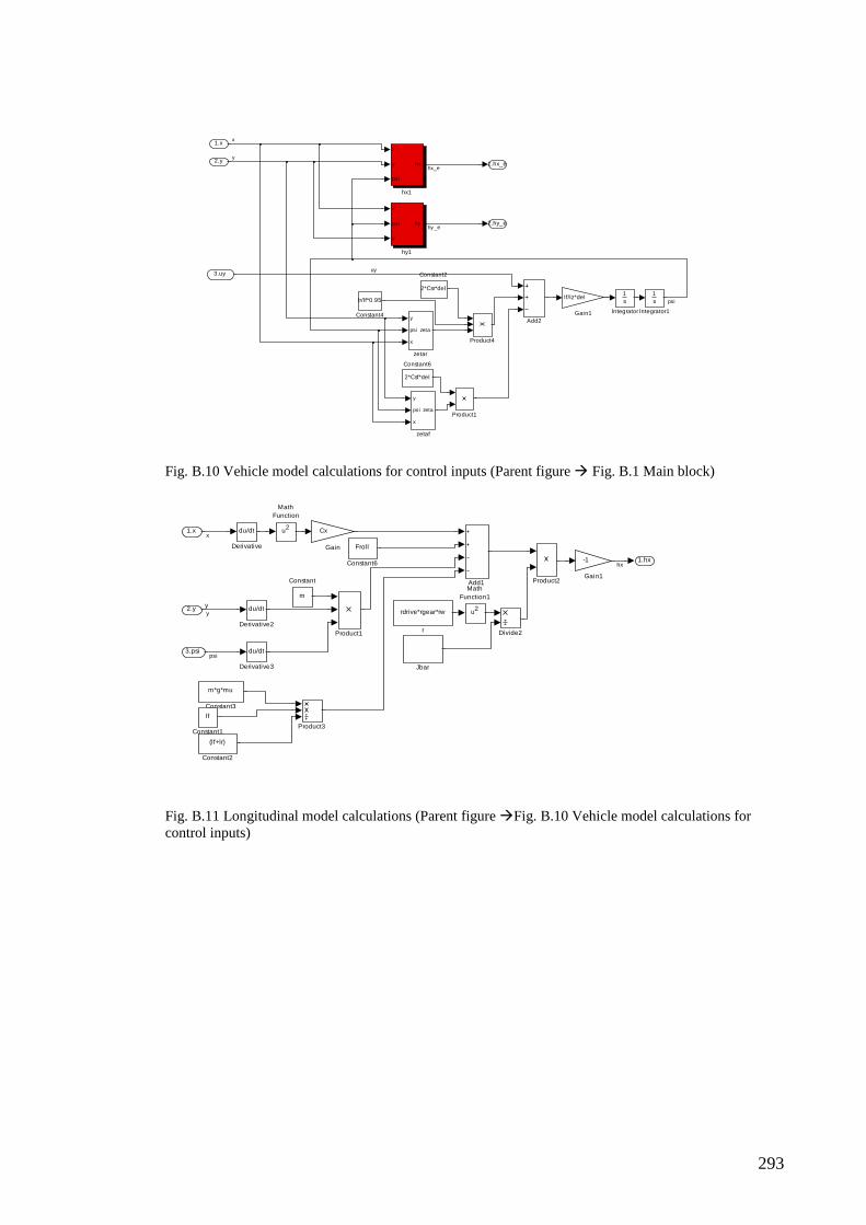
293
2.hy_e
1.hx_e
y
psi
x
zeta
zetar
y
psi
x
zeta
zetaf
x
psi
y
hy
hy1
x
y
psi
hx
hx1
Product4
Product1
1s
Integrator1
1s
Integrator
lf/Iz*del
Gain1
2*Csf*del
Constant6
lr/lf*0.95
Constant4
2*Csr*del
Constant2
Add2
3.uy
2.y
1.x
psi
uy
x
y
hy _e
hx_e
Fig. B.10 Vehicle model calculations for control inputs (Parent figure Fig. B.1 Main block)
y
1.hx
rdrive*rgear*rw
r
Product3
Product2
Product1
u2
MathFunction1
u2
MathFunction
Jbar
-1
Gain1
Cx
Gain
Divide2
du/dt
Derivative3
du/dt
Derivative2
du/dt
Derivative Frol l
Constant6
m*g*mu
Constant3
(lf+lr)
Constant2
lf
Constant1
m
Constant Add1
3.psi
2.y
1.x
hx
psi
y
x
Fig. B.11 Longitudinal model calculations (Parent figure Fig. B.10 Vehicle model calculations for control inputs)

294
1.hy
y
psi
x
zeta
zetar
y
psi
x
zeta
zetaf Product3
Product2
Product1
u2
MathFunction
-1/m
Gain1
Cy
Gain
du/dt
Derivative3
du/dt
Derivative2
du/dt
Derivative
2*Csf
Constant3
2*Csr
Constant2
m
Constant
Add1
3.y
2.psi
1.x
y
hy
psi
psi
x
Fig. B.12 Lateral model calculations (Parent figure Fig. B.10 Vehicle model calculations for control inputs)
1
Out1
GX2
To Workspace2
MX2
To Workspace1
Z2
To Workspace
-K-
Scaler Factor2
-K-
Scaler Factor1-K-
Scaler Factor
u
v
t
f
Z2
MX2
GX2
afuzzy
EmbeddedMATLAB Function
du/dt
Derivative
0
Clock
1
In1
Fig. B.13 Adaptive fuzzy controller-longitudinal (Parent figure Fig. B.1 Main block)
1
Out1
GX1
To Workspace2
MX1
To Workspace1
Z1
To Workspace
-K-
Scaler Factor2
-K-
Scaler Factor1-K-
Scaler Factor
u
v
t
f
Z1
MX1
GX1
afuzzy
EmbeddedMATLAB Function
du/dt
Derivative
0
Clock
1
In1
Fig. B.14 Adaptive fuzzy controller-lateral (Parent figure Fig. B.1 Main block)
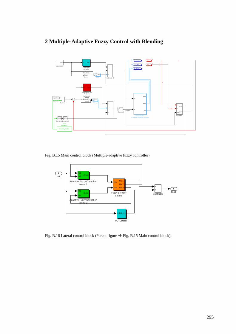
295
2 Multiple-Adaptive Fuzzy Control with Blending
3.<delta>
2.<Fpr>
1.<alpha>
Out1
lateral error
In1In2Out1
VSlong
In1In2Out1
VSlat Subtract3 2
Subtract2
Subtract
x
y
<uy 1>
hx_e
hy _e
Subsystem
In1 Out1
Longitudinal MMControl ler
In1 Out1
Lateral MM Control ler
uy
ux
alpha
delta
Fpr
Inverse Model for Vehicle Input Calculations
leaddist_accdcc
FromWorkspace
du/dt
Derivative8
du/dt
Derivative3
du/dt
Derivative2
du/dt
Derivative1
xspacing
Constant
2.y
1.x
LongInput
y
y
y
y
x
xx
x
Fig. B.15 Main control block (Multiple-adaptive fuzzy controller)
1
Out1Subtract1
In1Out1
PD_Lateral
In1
In2
Out1
Out2
Out3
Fuzzy BlenderLataral
In1
In2Out1
Adaptive Fuzzy Controllerlateral 2
In1
In2 Out1
Adaptive Fuzzy Controllerlateral 1
1
In1
Fig. B.16 Lateral control block (Parent figure Fig. B.15 Main control block)

296
1
Out1Subtract4
In1Out1
PD Longitudinal
In1
In2
Out1
Out2
Out3
Fuzzy BlenderLongitudinal
In1
In2Out1
Adaptive Fuzzy Controllerlongitudinal 2
In1
In2Out1
Adaptive Fuzzy Controllerlongitudinal 1
1
In1
Fig. B.17 Longitudinal control block (Parent figure Fig. B.15 Main control block)
3
Out3
2
Out2
1
Out1
ZLatB
To Workspace2
u
v
t
f
f 1
f 2
Z
fuzzyblend
Lateral Fuzzy Blender
-K-
Gain3
-K-
Gain1
-K-
Gain
0
Clock
2
In2
1
In1
Fig. B.18 Fuzzy blender- lateral (Parent figure Fig. B.16 Longitudinal control block)
3
Out3
2
Out2
1
Out1
ZLBx
To Workspace2
-K-
Gain3
-K-
Gain1
-K-
Gain
u
v
t
f
f 1
f 2
Z
fuzzyblend
EmbeddedMATLAB Function1_4rule
0
Clock
2
In2
1
In1
Fig. B.19 Fuzzy blender-longitudinal (Parent figure Fig. B.17 Longitudinal control block)

297
3 Multiple-Model PDC-based Multiple-Adaptive Fuzzy Control with Blending
vx
Lat Input
3.<delta>
2.<Fpr>
1.<alpha>Out1
lateral error
Subtract
uy
ux
alpha
delta
Fpr
Solution for Inputs
long_error
xdot
psidot
xp
y dot
Out1
Longitudinal MM PDCController
lat_error
xdot
y dot
psidot
Out1
Lateral MM PDC Controller
leaddist_accdcc
FromWorkspace
du/dt
Derivative9du/dt
Derivative12
du/dt
Derivative11
xspacing
Constant
3.psi
2.y
1.x
psi
psi
y
x
LongInput
xdot
y dot
psidot
Fig. B.20 Main control block (Multiple-model PDC controller)
1
Out1-K-
scaler factor
xi1
x2
x6
xi2
xi3
xi4
rho_x_hat
Vehicle local models
In1Out1
Variable structure long
Subtract4
x2
x4
xi1
xi2
xi3
xi4
pdc
PDC Controller Longitudinal
In1Out1
PD Longitudinal
In1
In2 Out1
Long_4
In1
In2 Out1
Long_3
In1
In2 Out1
Long_2
In1
In2 Out1
Long_1
du/dt
Derivative17
du/dt
Derivative1
ux1
<xi1>
ux2
xi2
ux3
xi3
ux4
xi4
ux
Control Input Blending
5.ydot
4.xp
3.psidot
2.xdot
1.long_error
long_error
long_error
xi1
xi1xi1
xi2
xi2xi2
xi3
xi3
xi3
xi4
xi4
xi4
xdot
psidot
xp
y dot
Fig. B.21 Longitudinal control block (Parent figure Fig. B.20 Main control block)
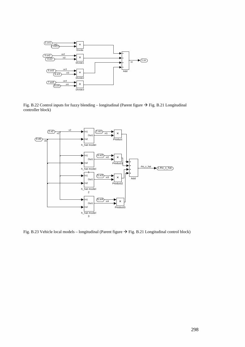
298
1.ux
Divide3
Divide2
Divide1
Divide
Add
8.xi4
7.ux4
6.xi3
5.ux3
4.xi2
3.ux2
2.<xi1>
1.ux1
xi2
xi3
xi4
ux1
ux2
ux
ux3
ux4
Fig. B.22 Control inputs for fuzzy blending – longitudinal (Parent figure Fig. B.21 Longitudinal controller block)
1.rho_x_hat
In1
In2
Out1
h_hat model3
In1
In2
Out1
h_hat model2
In1
In2
Out1
h_hat model1
In1
In2
Out1
h_hat model
Product3
Product2
Product1
Product
Add
6.xi4
5.xi3
4.xi2
3.x6
2.x2 1.xi1
x6
x2x2 xi1
xi2
rho_x_hat
xi3
xi4
Fig. B.23 Vehicle local models – longitudinal (Parent figure Fig. B.21 Longitudinal control block)

299
1
Out1
-K-
scaler factor
xi1
x4
x6
xi2
xi3
xi4
rho_y _
Vehicle local models
In1Out1
Variable structurelateral
Subtract1
x2
x4
xi1
xi2
xi3
xi4
pdc
PDC Control ler Lateral
In1Out1
PD Lateral
In1
In2 Out1
Lat_4
In1
In2 Out1
Lat_3
In1
In2 Out1
Lat_2
In1
In2 Out1
Lat_1
uy 1
<xi1>
uy 2
xi2
uy 3
xi3
uy 4
xi4
psitheta
Control Input Blending
4.psidot
3.ydot
2.xdot
1.lat_errorlat_error
lat_error
xi1
xi1
xi1
xi1
xi2
xi2
xi3
xi3
xi4
xi4xi4
xdot
y dot
psidot
Fig. B.24 Lateral control block (Parent figure Fig. B.20 Main control block)
1.psitheta
Divide3
Divide2
Divide1
Divide
Add
8.xi4
7.uy4
6.xi3
5.uy3
4.xi2
3.uy2
2.<xi1>
1.uy1
xi2
xi3
xi4
uy 1
uy 2
psitheta
uy 3
uy 4
Fig. B.25 Control inputs for fuzzy blending – lateral (Parent figure Fig. B.24 Lateral control block)
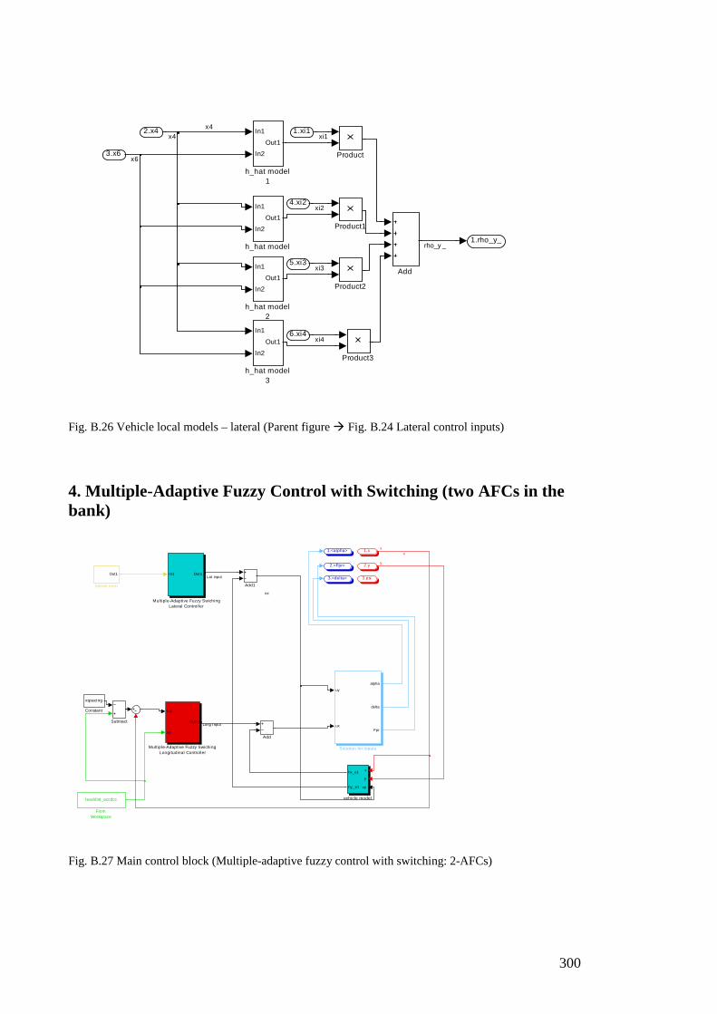
300
1.rho_y_
In1
In2
Out1
h_hat model3
In1
In2
Out1
h_hat model2
In1
In2
Out1
h_hat model1
In1
In2
Out1
h_hat model
Product3
Product2
Product1
Product
Add
6.xi4
5.xi3
4.xi2
3.x6
2.x4 1.xi1
x6
x4x4 xi1
xi2
rho_y _
xi3
xi4
Fig. B.26 Vehicle local models – lateral (Parent figure Fig. B.24 Lateral control inputs) 4. Multiple-Adaptive Fuzzy Control with Switching (two AFCs in the bank)
vx
3.<delta>
2.<Fpr>
1.<alpha>
x
y
uy
hx_e1
hy _e1
vehicle model
Out1
lateral error
Subtract
uy
ux
alpha
delta
Fpr
Solution for Inputs
In1
xp
Out1
Multiple-Adaptive Fuzzy SwichingLongitudinal Controller
leaddist_accdcc
FromWorkspace
xspacing
Constant
Add1
Add
In1 Out1
Multiple-Adaptive Fuzzy Swiching Lateral Control ler
3.psi
2.y
1.x
y
xx
Long Input
Lat input
Fig. B.27 Main control block (Multiple-adaptive fuzzy control with switching: 2-AFCs)

301
1
Out1
-K-
scaler factor
sq1
sq2
Out1
Out2
comparator
In1Out1
VSlong1
sq1
sq2
t
xi1
xi2
pdc
Switching Logic
Subtract1
In1Out1
PD Lateral
In1Out1
Out2
Lateral AFuzzy Controller 3
In1Out1
Out2
Lateral AFuzzy Control ler 2
uy 1
xi1
uy 2
xi2
psitheta
Controller Switcher - lateral
0
Clock
1
In1
xi2xi2
xi1
Fig. B.28 Multiple-adaptive fuzzy control with switching – lateral (Parent figure Fig. B.27 Main control block)
1
Out1
-K-
scaler factor
In1Out1
VSlong1
Subtract4
sq1
sq2
t
xi1
xi2
pdc
PDC ControllerSwitching logic
In1Out1
PD Longitudinal
In1Out1
Out2
Longitudinal AFuzzy Controller 3
In1Out1
Out2
Longitudinal AFuzzy Controller 2
du/dt
Derivative17
du/dt
Derivative1
sq2
sq3
Out2
Out3
Cost Function Comparator
ux1
xi1
ux2
xi2
ux
Controller Swicher - longitudinal
0
Clock
2.xp
1
In1
xp
xi1
xi2
Fig. B.29 Multiple-adaptive fuzzy control with switching – longitudinal (Parent figure Fig. B.27 Main control block)

302
2
Out2
1
Out1
In1 Out1
w2
In1 Out1
w1
==
RelationalOperator2
==
RelationalOperator1
min
MinMax
double
Data Type Conversion2
double
Data Type Conversion1
|u|
Abs2
|u|
Abs1
2.sq2
1.sq1sq1
sq2
Fig. B.30 Cost function comparator for switching (lateral/ longitudinal) (Parent figure Fig. B.28/ B.29 Multiple-adaptive fuzzy control with switching-lateral/longitudinal)
1.psitheta
Divide2
Divide1
Add4.xi2
3.uy2
2.xi1
1.uy1xi1
xi2
uy 1
psithetauy 2
Fig. B.31 Controller switcher (longitudinal/ lateral) (Parent figure Fig. B.28/ B.29 Multiple-adaptive fuzzy control with switching-longitudinal/lateral)
1
Out1
1s
Integrator
-K-
Gain1
-K-
Gain
du/dt
Derivative
Add|u|
Abs1
|u|
Abs
1
In1
Fig. B.32 Cost function for controller switching (w1 and w2) (Parent figure Fig. B.30 Multiple-adaptive switcher – lateral/longitudinal)

303
5. Multiple-Adaptive Fuzzy Control with Switching (four AFCs in the bank)
vx
3.<delta>
2.<Fpr>
1.<alpha>
x
y
uy
hx_e1
hy _e1
vehicle model
Out1
lateral error
Subtract
uy
ux
alpha
delta
Fpr
Solution for Inputs
leaddist_accdcc
FromWorkspace
xspacing
Constant
Add1
Add
In1
xp
Out1
MAF SwichingLongitudinal Controller
In1 Out1
MAF Swiching Lateral Controller
3.psi
2.y
1.x
y
xx
Long Input
Lat input
Fig. B.33 Main control block (Multiple-adaptive fuzzy control with switching: 4-AFCs)
1
Out1
-K-
scaler factor
In1Out1
VSlong1
sq1
sq2
sq3
sq4
t
xi1
xi2
xi3
xi4
pdc
Switching logic
Subtract4
In1Out1
PD Longitudinal
In1Out1
Out2
Longitudinal AFuzzy Control ler 4
In1Out1
Out2
Longitudinal AFuzzy Control ler 3
In1Out1
Out2
Longitudinal AFuzzy Control ler 2
In1Out1
Out2
Longitudinal AFuzzy Control ler 1
du/dt
Derivative17
du/dt
Derivative1
sq1
sq2
sq3
sq4
Out1
Out2
Out3
Out4
Cost Function Comparator
ux1
<xi1>
ux2
xi2
ux3
xi3
ux4
xi4
ux
Controller Swicher - longitudinal
0
Clock
2.xp
1
In1
xi1xi1
xi2
xi2
xi3
xi3
xi4
xi4
xp
Fig. B.34 Multiple-adaptive fuzzy control with switching – longitudinal (Parent figure Fig. B.33 Main control block)

304
4
Out4
3
Out3
2
Out2
1
Out1
In1Out1
w4
In1 Out1
w3
In1 Out1
w2
In1 Out1
w1
==
RelationalOperator3
==
RelationalOperator2
==
RelationalOperator1
==
RelationalOperator
min
MinMax
double
Data Type Conversion3
double
Data Type Conversion2
double
Data Type Conversion1
double
Data Type Conversion
|u|
Abs3
|u|
Abs2
|u|
Abs1
|u|
Abs
4.sq4
3.sq3
2.sq2
1.sq1sq1
sq2
sq3
sq4
Fig. B.35 Cost function comparator for switching – longitudinal (Parent figure Fig. B.34 Multiple- adaptive fuzzy control with switching – longitudinal)
1.ux
Divide3
Divide2
Divide1
Divide
Add
8.xi4
7.ux4
6.xi3
5.ux3
4.xi2
3.ux2
2.<xi1>
1.ux1
xi2
xi3
xi4
ux1
ux2
uxux3
ux4
Fig. B.36 Controller switcher – longitudinal (Parent figure Fig. B.34 Multiple-adaptive fuzzy control with switching – longitudinal)

305
1
Out1
-K-
scaler factor
sq1
sq2
sq3
sq4
Out1
Out2
Out3
Out4
comparator
In1Out1
VSlong1
Subtract1
In1Out1
PD Lateral
In1Out1
Out2
Lateral AFuzzy Controller 4
In1Out1
Out2
Lateral AFuzzy Controller 3
In1Out1
Out2
Lateral AFuzzy Controller 2
In1Out1
Out2
Lateral AFuzzy Controller 1
uy 1
<xi1>
uy 2
xi2
uy 3
xi3
uy 4
xi4
psitheta
Controller Switcher - lateral
0
Clock
sq1
sq2
sq3
sq4
t
xi1
xi2
xi3
xi4
pdc
Switching Logic
1
In1
xi1
xi1
xi2
xi3
xi4
xi4
Fig. B.37 Multiple-adaptive fuzzy control with switching – lateral (Parent figure Fig. B.33 Main control block)
4
Out4
3
Out3
2
Out2
1
Out1
In1 Out1
w4
In1 Out1
w3
In1 Out1
w2
In1 Out1
w1
==
RelationalOperator3
==
RelationalOperator2
==
RelationalOperator1
==
RelationalOperator
min
MinMax
double
Data Type Conversion3
double
Data Type Conversion2
double
Data Type Conversion1
double
Data Type Conversion
|u|
Abs3
|u|
Abs2
|u|
Abs1
|u|
Abs
4.sq4
3.sq3
2.sq2
1.sq1sq1
sq2
sq3
sq4
Fig. B.38 Cost function comparator for switching – lateral (parent figure Fig. B.37 Multiple-adaptive fuzzy control with switching–lateral)
1.psitheta
Divide3
Divide2
Divide1
Divide
Add
8.xi4
7.uy4
6.xi3
5.uy3
4.xi2
3.uy2
2.<xi1>
1.uy1
xi2
xi3
xi4
uy 1
uy 2
psitheta
uy 3
uy 4
Fig. B.39 Controller switcher–lateral (Parent figure Fig. B.37 Multiple-adaptive fuzzy control with switching–lateral)

306
Appendix C Trained Parameters of Fuzzy Systems 1. Single-Adaptive Fuzzy Control Structure The trained T–S fuzzy membership function parameters are as follows
(i) Lateral Control :
The tuned Gaussian fuzzy input membership functions are as follows: ‘error’ variable:
1
2 2( ) exp( ( 0.002) / 0.021 )A
x xµ = − − , 0.002x ≥ or 1 ( ) 1A
xµ = , 0.002x <
2
2 2( ) exp( ( 0.002511) / 0.0003198 )A
x xµ = − − (C.1)
3
2 2( ) exp( ( 0.006) / 0.018 )A
x xµ = − − , 0.002x ≤ or 3 ( ) 1A
xµ = , 0.002x >
‘error rate’ variable:
1
2 2( ) exp( ( 0.095) / 0.039 )A
x xµ = − + , 0.095x ≥ − or 1 ( ) 1A
xµ = , 0.095x < −
2
2 2( ) exp( ( 0.02323) / 0.03457 )A
x xµ = − − (C.2)
3
2 2( ) exp( ( 0.110) / 0.032 )A
x xµ = − − , 0.11x ≤ or 3 ( ) 1A
xµ = , 0.110x > .
The tuned T–S fuzzy output membership functions a priori are as follows,
1 2.999e 006 2.972e 005z e e= − + − + ɺ
2 2.999e 006 2.972e 005z e e= − + − + ɺ
3 3.001e 006 2.98e 005z e e= − + − + ɺ
4 3.002e 006 2.987e 005z e e= − + − + ɺ
5 3.002e 006 2.986e 005z e e= − + − + ɺ
6 2.997e 006 2.978e 005z e e= − + − + ɺ (C.3)
7 25.63 317.3z e e= − + ɺ
8 7843 3.422e 004z e e= − − + ɺ
9 305.2 898.4 .z e e= − − ɺ

307
(ii) Longitudinal Control :
The tuned Gaussian input fuzzy membership functions are as follows: ‘error’ variable:
1
2 2( ) exp( ( 5.066) / 2.14 )A
x xµ = − +,
5.066x ≥ − or 1 ( ) 1A
xµ =,
5.066x < −
2
2 2( ) exp( ( 2.748) / 2.573 )A
x xµ = − +
3
2 2( ) exp( ( 0.2756) / 2.505 )A
x xµ = − + (C.4)
4
2 2( ) exp( ( 4.663) / 0.5623 )A
x xµ = − −
5
2 2( ) exp( ( 9.370) / 2.406 )A
x xµ = − −, 9.370x ≤
or 5 ( ) 1A
xµ =,
9.370x >,
‘error rate’ variable:
1
2 2( ) exp( ( 7.822) / 0.352 )A
x xµ = − +, 7.822x ≥ −
or 1 ( ) 1A
xµ =,
7.822x < −
2
2 2( ) exp( ( 1.394) /1.336 )A
x xµ = − +
3
2 2( ) exp( ( 1.006) /1.313 )A
x xµ = − −
4
2 2( ) exp( ( 3.210) /1.1 )A
x xµ = − − (C.5)
5
2 2( ) exp( ( 8.524) / 0.6871 )A
x xµ = − −, 8.524x ≤
or 5 ( ) 1
Axµ =
,8.524x >
. The tuned output T–S fuzzy membership function parameters a priori are as follows:
1 = 8941 3.172e 004 z e e− + ɺ
2 2.997e 005 3.001e 005 z e e= − + − + ɺ
3 2.981e 005 3.005e 005 z e e= − + − + ɺ
4 2.99e 005 2.997e 005 z e e= − + − + ɺ
5 4.848e 004 8.951e 004 z e e= + − + ɺ
6 = 8.107e+004 3.329e 005 z e e− − + ɺ
7 = 2.964e+005 3e 005 z e e− − + ɺ
8 2.869e 005 2.998e 005 z e e= − + − + ɺ
9 2.861e 005 3.002e 005 z e e= − + − + ɺ
10 2.252e 004 2.678e 005 z e e= − + − + ɺ
11 2.648e 005 2.522e 005 z e e= − + − + ɺ
12 2.987e 005 3e 005 z e e= − + − + ɺ
13 2.967e 005 3.001e 005 z e e= − + − + ɺ (C.6)
14 2.948e 005 2.999e 005 z e e= − + − + ɺ

308
15 2.798e 005 3.246e 005 z e e= − + − + ɺ
16 2.987e 005 3.006e 005 z e e= − + − + ɺ
17 6.671e 004 8.401e 004 z e e= − + − + ɺ
18 1.508 12.57 z e e= − − ɺ
19 408.4 368.6 z e e= − − ɺ
20 2.99e 005 2.973e 005 z e e= − + − + ɺ
21 2.991e 005 2.999e 005 z e e= − + − + ɺ
22 3e 005 3e 005 z e e= − + − + ɺ
23 3.001e 005 3e 005 z e e= − + − + ɺ
24 3e 005 3e 005 z e e= − + − + ɺ
25 2.969e 005 2.947e 005 . z e e= − + − + ɺ
2. Multiple-Adaptive Fuzzy Controller with Fuzzy Blender
Fuzzy Blender Parameters for Final Trial
(i) Longitudinal Controller:
(a) Input Membership Function Parameters:
Input variable: Controller #1
1
2 2( ) exp( ( 71.11) /13.45 )A
x xµ = − +
2
2 2( ) exp( ( 41.13) /13.44 )A
x xµ = − + (C.7)
3
2 2( ) exp( ( 2.023) /13.61 )A
x xµ = − +
4
2 2( ) exp( ( 0.006218) /13.44 )A
x xµ = − +
Input variable: Controller #2
1
2 2( ) exp( ( 71.13) /13.45 )A
x xµ = − +
2
2 2( ) exp( ( 41.11) /13.45 )A
x xµ = − +
3
2 2( ) exp( ( 1.816) /13.44 )A
x xµ = − +
4
2 2( ) exp( ( 0.00376) /13.45 )A
x xµ = − + (C.8)

309
(b) Output Membership Function Parameters:
1 1 24.238 4.246 z C C= − 2 1 219.49 15.91 z C C= + 3 1 21.07 1.074 z C C= − − 4 1 23.291 3.293 z C C= − − 5 1 215.95 19.52 z C C= − − 6 1 22.191 2.428 z C C= − 7 1 228.54 28.57 z C C= + 8 1 22.447 2.379 z C C= − − 9 1 20.1276 0.1227 z C C= + 10 1 221.14 21.37 z C C= − − 11 1 24.091 3.964 z C C= − 12 1 27.113 1.022 z C C= − 13 1 23.333 3.336 z C C= − − 14 1 24.117 4.31 z C C= − − 15 1 21.995 7.515 z C C= − 16 1 24.498 5.066 z C C= − (C.9)
(ii) Lateral Controller:
(a) Input Membership Function Parameters:
Input variable: Controller #1
1
2 2( ) exp( ( 36.11) / 20.6 )A
x xµ = − +
2
2 2( ) exp( ( 27.77) / 20.6 )A
x xµ = − − (C.10)
Input variable: Controller #2
1
2 2( ) exp( ( 42.78) / 20.5 )A
x xµ = − +
2
2 2( ) exp( ( 35.33) / 20.5 )A
x xµ = − − (C.11)
(b) Output Membership Function Parameters:
1 1 20.05 0.076 z C C= +
2 1 20.034 0.043 z C C= +
3 1 20.1129 0.1133 z C C= − +
4 1 20.09751 0.09795 z C C= − + (C.12)

310
3. Multiple-Model PDC-based Multiple-Adaptive Fuzzy Structure
Parameters for the Individual Adaptive Fuzzy Controllers
(i) Lateral Control:
1. controller #1 (data obtained when 2 35x = , 4 1x = ) Input Gaussian function parameters: ‘error’ variable
1
2 2( ) exp( ( 0.0724) / 0.2031 )A
x xµ = − − (C.13)
2
2 2( ) exp( ( 0.441 ) / 0.1974 )A
x xµ = − −
‘error rate’ variable
1
2 2( ) exp( ( 0.01726) / 0.0195 )A
x xµ = − − (C.14)
2
2 2( ) exp( ( 0.05816 ) / 0.06497 )A
x xµ = − −
T–S Fuzzy Output Membership Function Parameters: 1 = 4671 2.732e 004 z e e− + + ɺ
2 = 8724 4.857e 004 z e e− + ɺ
3 = 1851 4228 z e e− + ɺ
4 = 3001 2588 z e e− ɺ (C.15)
311
2. controller #2 (data obtained when 2 35x = , 4 1x = − )
Input Gaussian function parameters: ‘error’ variable
1
2 2( ) exp( ( 0.4425) / 0.198 )A
x xµ = − + (C.16)
2
2 2( ) exp( ( 0.0727 ) / 0.2038 )A
x xµ = − +
‘error rate’ variable
1
2 2( ) exp( ( 0.01725) / 0.0195 )A
x xµ = − − (C.17)
2
2 2( ) exp( ( 0.05817 ) / 0.06497 )A
x xµ = − −
T–S Fuzzy Output Membership Function Parameters:
1 = 1865 4226 z e e− − ɺ
2 = 2988 2583 z e e+ ɺ (C.18)
3 = 4644 2.731e 004 z e e− − + ɺ
4 = 8692 4.857e 004 z e e+ + ɺ
3. controller #3 (data obtained when 2 5x = − , 4 1x = )
Input Gaussian function parameters: ‘error’ variable
1
2 2( ) exp( ( 0.007666) / 0.01307 )A
x xµ = − − (C.19)
2
2 2( ) exp( ( 0.03459) / 0.04349 )A
x xµ = − −
‘error rate’ variable
1
2 2( ) exp( ( 0.03945) / 0.04414 )A
x xµ = − −
2
2 2( ) exp( ( 0.0789) / 0.02361 )A
x xµ = − − (C.20)

312
T–S Fuzzy Output Membership Function Parameters:
1 = 5175 6.181e 004 z e e− + ɺ
2 = 7424 1.364e 004 z e e− − + ɺ (C.21)
3 = 7165 4.996e 004 z e e− + ɺ
4 = 7432 1.133 004 z e e e+ + ɺ
4. controller #4 (data obtained when 2 5x = − , 4 1x = − )
Input Gaussian function parameters: ‘error’ variable
1
2 2( ) exp( ( 0.0724) / 0.2031 )A
x xµ = − − (C.22)
2
2 2( ) exp( ( 0.441) / 0.1974 )A
x xµ = − −
‘error rate’ variable
1
2 2( ) exp( ( 0.05816) / 0.06497 )A
x xµ = − − (C.23)
2
2 2( ) exp( ( 0.01726) / 0.0195 )A
x xµ = − −
T–S Fuzzy Output Membership Function Parameters:
1 = 4671 2.732e 004 z e e− + + ɺ
2 = 8724 4.857e 004 z e e− + ɺ (C.24)
3 = 1851 4228 z e e− + ɺ
4 = 3001 2588 z e e− ɺ
313
(ii) Longitudinal Control:
1. controller #1 (data obtained when 2 35x = , 4 1x = )
Input Gaussian function parameters: ‘error’ variable
1
2 2( ) exp( ( 23.19) / 22.83 )A
x xµ = − + (C.25)
2
2 2( ) exp( ( 7.211) / 23.02 )A
x xµ = − +
‘error rate’ variable
1
2 2( ) exp( ( 12.14) / 4.44 )A
x xµ = − + (C.26)
2
2 2( ) exp( ( 0.4308) / 3.797 )A
x xµ = − −
T–S Fuzzy Output Membership Function Parameters:
1 = 0.0424 0.09198 z e e− − ɺ
2 = 0.2779 0.3019 z e e+ ɺ (C.27)
3 = 0.07343 0.1432 z e e− + ɺ
4 = 0.01449 0.1136 z e e− ɺ
2. controller #2 (data obtained when2 35x = , 4 1x = − )
Input Gaussian function parameters: ‘error’ variable
1
2 2( ) exp( ( 38.25) / 23 )A
x xµ = − + (C.28)
2
2 2( ) exp( ( 4.77) / 23.03 )A
x xµ = − −
‘error rate’ variable
1
2 2( ) exp( ( 12.05) / 7.35 )A
x xµ = − + (C.29)
2
2 2( ) exp( ( 7.566) / 8.532 )A
x xµ = − +

314
T–S Fuzzy Output Membership Function Parameters:
1 = 0.3259 3912 z e e− + ɺ
2 = 0.4104 0.2188 z e e+ ɺ (C.30)
3 = 0.03978 0.02231 z e e− + ɺ
4 = 0.07179 0.08603 z e e+ ɺ
3. controller #3 (data obtained when2 5x = − , 4 1x = ) Input Gaussian function parameters: ‘error’ variable
1
2 2( ) exp( ( 35.29) / 38.56 )A
x xµ = − − (C.31)
2
2 2( ) exp( ( 90.9) / 38.54 )A
x xµ = − −
‘error rate’ variable
1
2 2( ) exp( ( 8.994) / 2.301 )A
x xµ = − − (C.32)
2
2 2( ) exp( ( 13.98) /1.649 )A
x xµ = − −
T–S Fuzzy Output Membership Function Parameters:
1 = 0.01506 1.464 z e e− + ɺ
2 = 0.405 9.919 z e e− ɺ (C.33)
3 = 0.04345 2.491 z e e− − ɺ
4 = 0.5207 3.48 z e e− + ɺ
4. controller #4 (data obtained when2 5x = − , 4 1x = − ) Input Gaussian function parameters: ‘error’ variable
1
2 2( ) exp( ( 38.25) / 23 )A
x xµ = − + (C.34)
2
2 2( ) exp( ( 4.77) / 23.03 )A
x xµ = − −

315
‘error rate’ variable
1
2 2( ) exp( ( 12.05) / 7.35 )A
x xµ = − +
2
2 2( ) exp( ( 7.566) / 8.532 )A
x xµ = − + (C.35)
T–S Fuzzy Output Membership Function Parameters:
1 = 0.3259 0.3912 z e e− + ɺ
2 = 0.4104 0.2189 z e e+ ɺ (C.36)
3 = 0.03977 0.0223 z e e− + ɺ
4 = 0.07178 0.08601 z e e+ ɺ
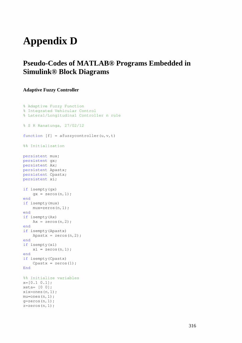
316
Appendix D
Pseudo-Codes of MATLAB® Programs Embedded in Simulink® Block Diagrams
Adaptive Fuzzy Controller
% Adaptive Fuzzy Function % Integrated Vehicular Control % Lateral/Longitudinal Controller n rule % S R Ranatunga, 27/02/12 function [f] = afuzzycontroller(u,v,t) %% Initialization persistent mux; persistent gx; persistent Ax; persistent Apastx; persistent Cpastx; persistent xi; if isempty(gx) gx = zeros( n,1); end if isempty(mux) mux=zeros( n,1); end if isempty(Ax) Ax = zeros( n,2); end if isempty(Apastx) Apastx = zeros( n,2); end if isempty(xi) xi = zeros( n,1); end if isempty(Cpastx) Cpastx = zeros(1); End %% Initialize variables x=[0.1 0.1]; xeta= [0 0]; xix=ones( n,1); mu=ones( n,1); g=zeros( n,1); z=zeros( n,1);

317
% Initialise output membership function parameters A=[ 1.5 1.5; 1.5 1.5; .
.
.
1.5 1.5; 1.5 1.5]; Sigmapastx=0.8; Sigmapast=0.1; % Set number of inputs and rules n=2; gain=0.1; % Output membership function parameters a priori: example values only Apast=[0.51 -0.35; 1.57 0.5;
.
.
.
-0.01 0.002; 4.31 7.21]; lambda=0.01; %%%%%%%%%%%%%% if (t<0.0002) Ax=A; Apastx=Apast; mux=mu; gx=g; Cpastx=Cpast; Sigmapastx=Sigmapast; xi=xix; end %%%%%%%%%%%%%%% x(1)=u; x(2)=v; %% For error variable c11= 0.001; c12= 0.0035; c13= 0.00058;
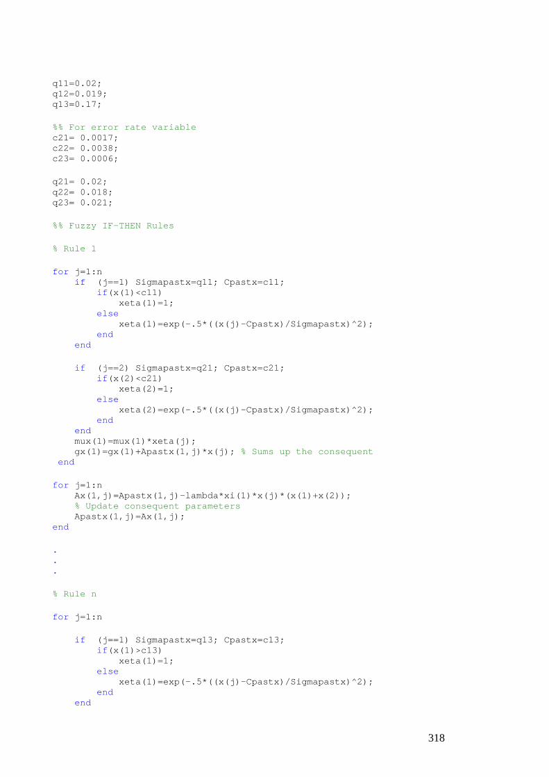
318
q11=0.02; q12=0.019; q13=0.17; %% For error rate variable c21= 0.0017; c22= 0.0038; c23= 0.0006; q21= 0.02; q22= 0.018; q23= 0.021; %% Fuzzy IF-THEN Rules % Rule 1 for j=1:n if (j==1) Sigmapastx=q11; Cpastx=c11; if (x(1)<c11) xeta(1)=1; else xeta(1)=exp(-.5*((x(j)-Cpastx)/Sigmapas tx)^2); end end if (j==2) Sigmapastx=q21; Cpastx=c21; if (x(2)<c21) xeta(2)=1; else xeta(2)=exp(-.5*((x(j)-Cpastx)/Sigmapas tx)^2); end end mux(1)=mux(1)*xeta(j); gx(1)=gx(1)+Apastx(1,j)*x(j); % Sums up the consequent end for j=1:n Ax(1,j)=Apastx(1,j)-lambda*xi(1)*x(j)*(x(1)+x(2 )); % Update consequent parameters Apastx(1,j)=Ax(1,j); end . . . % Rule n for j=1:n if (j==1) Sigmapastx=q13; Cpastx=c13; if (x(1)>c13) xeta(1)=1; else xeta(1)=exp(-.5*((x(j)-Cpastx)/Sigmapas tx)^2); end end

319
if (j==2) Sigmapastx=q23; Cpastx=c23 ; if (x(2)>c23) xeta(2)=1; else xeta(2)=exp(-.5*((x(j)-Cpastx)/Sigmapas tx)^2); end end mux( n)=mux( n)*xeta(j); gx( n)=gx( n)+Apastx( n,j)*x(j); % Sums up the consequent end for j=1:n Ax( n,j)=Apastx( n,j)-lambda*xi( n)*x(j)*(x(1)+x(2)); % Update consequent parameters Apastx( n,j)=Ax( n,j); end den=sum(mux(:)); % Denominator of xi for kth training data if (den ~= 0) xi=mux(:)/den; % Compute xi vector for kth training data pair else xi=zeros( n,1); end f=gx(:)'*xi(:); % Compute output for current training data end
Adaptive Fuzzy Controller in blender setup
% Adaptive Fuzzy Function % Integrated Vehicular Control % Multiple Adaptive Fuzzy Blending Scheme% Lateral/ Longitudinal Controller n rule % S R Ranatunga function [f] = afuzzycontroller(u,v,t,F) %% Initialization persistent mux; persistent gx; persistent Ax; persistent Apastx; persistent Cpastx; persistent xi; if isempty(gx) gx = zeros( n,1); end if isempty(mux)

320
mux=zeros( n,1); end if isempty(Ax) Ax = zeros( n,2); end if isempty(Apastx) Apastx = zeros( n,2); end if isempty(xi) xi = zeros( n,1); end if isempty(Cpastx) Cpastx = zeros(1); end %% Initialize variables x=[0.1 0.1]; xeta= [0 0]; xix=ones( n,1); mu=ones( n,1); g=zeros( n,1); z=zeros( n,1); % Initialise output membership function parameters A=[ 1.5 1.5; 1.5 1.5; 1.5 1.5; 1.5 1.5; 1.5 1.5; 1.5 1.5; 1.5 1.5; 1.5 1.5; 1.5 1.5]; Sigmapastx=0.8; Sigmapast=0.1; % Set number of inputs and rules n=2; gain=0.1; Apast=[1.5 1.5; 1.5 1.5; 1.5 1.5; 1.5 1.5; 1.5 1.5; 1.5 1.5; 1.5 1.5; 1.5 1.5; 1.5 1.5]; lambda=0.1; g1=0.2;
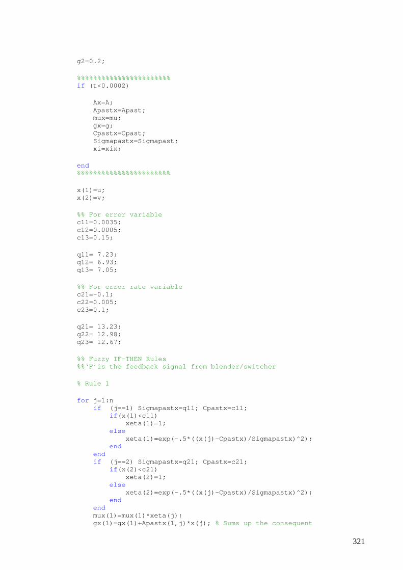
321
g2=0.2; %%%%%%%%%%%%%%%%%%%%%%% if (t<0.0002) Ax=A; Apastx=Apast; mux=mu; gx=g; Cpastx=Cpast; Sigmapastx=Sigmapast; xi=xix; end %%%%%%%%%%%%%%%%%%%%%%% x(1)=u; x(2)=v; %% For error variable c11=0.0035; c12=0.0005; c13=0.15; q11= 7.23; q12= 6.93; q13= 7.05; %% For error rate variable c21=-0.1; c22=0.005; c23=0.1; q21= 13.23; q22= 12.98; q23= 12.67; %% Fuzzy IF-THEN Rules %%‘F’is the feedback signal from blender/switcher % Rule 1 for j=1:n if (j==1) Sigmapastx=q11; Cpastx=c11; if (x(1)<c11) xeta(1)=1; else xeta(1)=exp(-.5*((x(j)-Cpastx)/Sigmapas tx)^2); end end if (j==2) Sigmapastx=q21; Cpastx=c21; if (x(2)<c21) xeta(2)=1; else xeta(2)=exp(-.5*((x(j)-Cpastx)/Sigmapas tx)^2); end end mux(1)=mux(1)*xeta(j); gx(1)=gx(1)+Apastx(1,j)*x(j); % Sums up the consequent

322
end for j=1:n Ax(1,j)=Apastx(1,j)-lambda*xi(1)*x(j)*F*(x(1)+x (2)); % Update consequent parameters Apastx(1,j)=Ax(1,j); end . . . % Rule n for j=1:n if (j==1) Sigmapastx=q13; Cpastx=c13; if (x(1)>c13) xeta(1)=1; else xeta(1)=exp(-.5*((x(j)-Cpastx)/Sigmapas tx)^2); end end if (j==2) Sigmapastx=q23; Cpastx=c23 ; if (x(2)>c23) xeta(2)=1; else xeta(2)=exp(-.5*((x(j)-Cpastx)/Sigmapas tx)^2); end end mux( n)= mux( n)*xeta(j); gx( n)=gx( n)+Apastx( n,j)*x(j); % Sums up the consequent end for j=1:n Ax( n,j)=Apastx( n,j)-lambda*xi( n)*x(j)*F*(x(1)+x(2)); % Update consequent parameters Apastx( n,j)=Ax( n,j); end %% Defuzzification den=sum(mux(:)); % Denominator of xi for kth training data if (den ~= 0) xi=mux(:)/den; % Compute xi vector for kth training data pair else xi=zeros( n,1); end f=gx(:)'*xi(:); % Compute output for the current training data end
Fuzzy Blending for Controllers

323
% Adaptive Fuzzy Function_final % Integrated Vehicular Control % Multiple Adaptive Fuzzy Controllers with Blender % Lateral/Longitudinal Blender -4 Rule % S R Ranatunga, 10/03/12 function [f,f1,f2,Z] = fuzzyblend(u,v,t) persistent mux; persistent gx; persistent Cpastx; persistent xi; f11=0; f22=0; if isempty(gx) gx = zeros(4,1); end if isempty(mux) mux=zeros(4,1); end if isempty(xi) xi = zeros(4,1); end if isempty(Cpastx) Cpastx = zeros(1); end %% Initialize variables x=[0.1 0.1 ]'; xeta=[0 0]; mu=ones(4,1); g=zeros(4,1); z=zeros(4,1); % Set number of inputs and rules n=2; Apast=[ -0.5056 0.5032 ; - 2.001 2.032 1.717 -1.748 -0.1122 0.1125]; Sigmapastx= 0.8; Sigmapast=0.1; mux=mu; gx=g;

324
x(1)=u; x(2)=v; %% 1st Fuzzy Controller c11 = -3.362e+004; c12 =-9.133; q11= 7811; q12= 7811; %% 2nd Fuzzy Controller c21 = -3.334e+004; c22 = -9.014; q21= 7795; q22= 7794; %% Fuzzy Blender IF-THEN Rules %1 Rule for j=1:n if (j==1) Cpastx=c11; Sigmapastx=q11; if (x(1)<c11) xeta(1)=1; else xeta(1)=exp(-.5*((x(j)-Cpastx)/Sigmapas tx)^2); end end if (j==2) Cpastx=c21; Sigmapastx=q21 if (x(2)<c21) xeta(2)=1; else xeta(2)=exp(-.5*((x(j)-Cpastx)/Sigmapas tx)^2); end end mux(1)=mux(1)*xeta(j); gx(1)=gx(1)+ Apast(1,j)*x(j); % Sum up the consequent end . . . %4 for j=1:n if (j==1) Cpastx=c12; Sigmapastx=q12; if (x(1)>c12) xeta(1)=1; else xeta(1)=exp(-.5*((x(j)-Cpastx)/Sigmapas tx)^2); end end if (j==2) Cpastx=c22 ; Sigmapastx=q22; if (x(2)>c22) xeta(2)=1; else xeta(2)=exp(-.5*((x(j)-Cpastx)/Sigmapas tx)^2); end end

325
mux(4)=mux(4)*xeta(j); gx(4)=gx(4)+ Apast(4,j)*x(j); % Sum up the consequent end %% Defuzzification for j=1:4 z(j)=mux(j)*gx(j); end Z=z(:); den=sum(mux(:)); % Denominator of xi for kth training data if (den ~= 0) xi=mux(:)/den; % Compute xi vector for kth training data pair else xi=zeros(4,1); end f=gx(:)'*xi(:); % Compute the output for the current training data for j=1:4 f11=f11+ (mux(j)/den)*Apast(j,1); f22=f22+ (mux(j)/den)*Apast(j,2); end f1=f11; f2=f22; mux=ones(4,1); gx=zeros(4,1); end
Fuzzy PDC based Blender
% Adaptive Fuzzy Function_final % Integrated Vehicular Control % PDC structure for vehicle control % S R Ranatunga, 16/06/12 function [xi1, xi2, xi3, xi4] = pdc(x2, x4) persistent k1; persistent k2; persistent k3; persistent k4; if isempty(k1) k1 = ones(1); end if isempty(k2) k2 = ones(1);
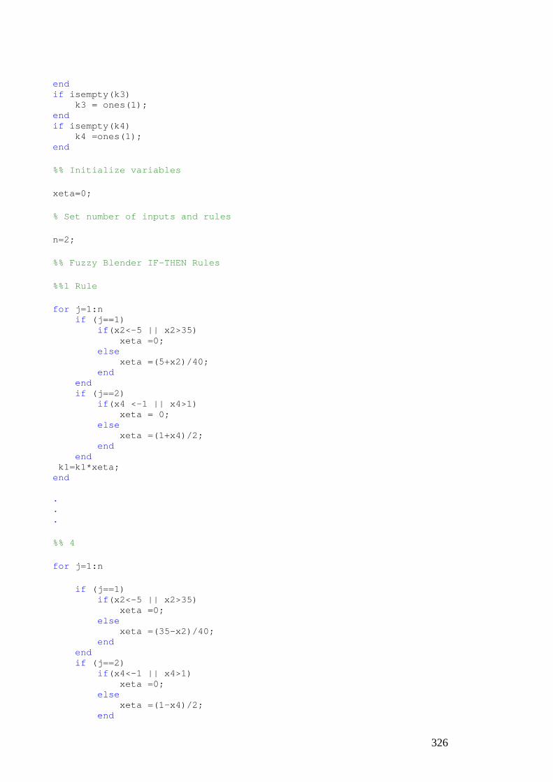
326
end if isempty(k3) k3 = ones(1); end if isempty(k4) k4 =ones(1); end %% Initialize variables xeta=0; % Set number of inputs and rules n=2; %% Fuzzy Blender IF-THEN Rules %%1 Rule for j=1:n if (j==1) if (x2<-5 || x2>35) xeta =0; else xeta =(5+x2)/40; end end if (j==2) if (x4 <-1 || x4>1) xeta = 0; else xeta =(1+x4)/2; end end k1=k1*xeta; end . . . %% 4 for j=1:n if (j==1) if (x2<-5 || x2>35) xeta =0; else xeta =(35-x2)/40; end end if (j==2) if (x4<-1 || x4>1) xeta =0; else xeta =(1-x4)/2; end

327
end k4=k4*xeta; end den = (k1+k2+k3+k4) ; if (den ~= 0) xi1=k1/den; xi2=k2/den; xi3=k3/den; xi4=k4/den; else xi1=zeros(1); xi2=zeros(1); xi3=zeros(1); xi4=zeros(1); end k1=ones(1); k2=ones(1); k3=ones(1); k4=ones(1); end Multiple-Adaptive Switcher (2-AFCs in the bank) % Switching Function % Integrated Vehicular Control % Multiple Adaptive Fuzzy Control with Switching (2 -AFCs) % S R Ranatunga, 16/06/12 function [xi1,xi2] = mas2(sq1,sq2,t) persistent k1; persistent k2; persistent tck; if isempty(tck) tck = zeros(1); end if isempty(k1) k1 = zeros(1); end if isempty(k2) k2 = zeros(1); end %% Time gap between switching t0=0.1e-2; %%initial setting if (t<t0) xi1=1; xi2=0; end %% Swithing if (sq1==1) if (t>=tck+t0) k1=sq1,k2=0,tck=t;

328
end elseif (sq2==1) if (t>=tck+t0) k1=0,k2=sq2,tck=t; end end %%Output values xi1=k1; xi2=k2; end
Multiple-Adaptive Switcher (4-AFCs in the bank)
% Switching Function % Integrated Vehicular Control % Multiple Adaptive Fuzzy Control with Switching (4 -AFCs) % S R Ranatunga, 16/06/12 function [xi1,xi2,xi3,xi4] = mas4(sq1,sq2,sq3,sq4,t) persistent k1; persistent k2; persistent k3; persistent k4; persistent tck; if isempty(tck) tck = zeros(1); end if isempty(k1) k1 = zeros(1); end if isempty(k2) k2 = zeros(1); end if isempty(k3) k3 = zeros(1); end if isempty(k4) k4 = zeros(1); end %% Time gap between switching t0=0.1e-2; %%Initial setting if (t<t0) xi1=1, xi2=0, xi3=0, xi4=0; end %% Switching if (sq1==1) if (t>=tck+t0) k1=sq1, k2=0, k3=0, k4=0,tck=t; end

329
elseif (sq2==1) if (t>=tck+t0) k1=0, k2=sq2, k3=0, k4=0, tck=t; end elseif (sq3==1) if (t>=tck+t0) k1=0, k2=0, k3=sq3, k4=0, tck=t; end elseif (sq4==1) if (t>=tck+t0) k1=0, k2=0, k3=0, k4=sq4, tck=t; end end %% Output values xi1=k1; xi2=k2; xi3=k3; xi4=k4; end


![Workplace Redefined[1]](https://static.fdocuments.in/doc/165x107/541c69077bef0a16088b4852/workplace-redefined1.jpg)