Adaptive Finite Element Methods Lecture 6: Adaptive …€¦ · Claudio Canuto, Politecnico di...
82
Adaptive Finite Element Methods Lecture 6: Adaptive Fourier-Galerkin Methods Ricardo H. Nochetto Department of Mathematics and Institute for Physical Science and Technology University of Maryland, USA www2.math.umd.edu/ ˜ rhn Joint work with Claudio Canuto, Politecnico di Torino, Italy Marco Verani, Politecnico di Milano, Italy 7th Z¨ urich Summer School, August 2012 A Posteriori Error Control and Adaptivity
Transcript of Adaptive Finite Element Methods Lecture 6: Adaptive …€¦ · Claudio Canuto, Politecnico di...

Adaptive Finite Element MethodsLecture 6: Adaptive Fourier-Galerkin Methods
Ricardo H. Nochetto
Department of Mathematics andInstitute for Physical Science and Technology
University of Maryland, USAwww2.math.umd.edu/˜rhn
Joint work with
Claudio Canuto, Politecnico di Torino, Italy
Marco Verani, Politecnico di Milano, Italy
7th Zurich Summer School, August 2012A Posteriori Error Control and Adaptivity

Outline Introduction Sparsity Fourier-Galerkin Methods Feasible ADFOUR Optimality
Outline
Introduction
Sparsity
Adaptive Fourier-Galerkin Methods
F-ADFOUR: Feasible ADFOUR
Optimality of Adaptive Algorithms
Adaptive Finite Element Methods Lecture 6: Adaptive Fourier-Galerkin Methods Ricardo H. Nochetto

Outline Introduction Sparsity Fourier-Galerkin Methods Feasible ADFOUR Optimality
Higher Order Methods: h-p Adaptivity
I A priori
[Dahmen and Scherer ’79,DeVore and Scherer ’79,Babuska and Guo 86’, 88’, 94’,Schwab ’98
... ],
I A posteriori
[Oden, Demkowicz et al ’89,Bernardi ’96,Ainsworth and Senior ’98,Schmidt and Siebert ’00,Melenk and Wohlmuth ’01,Heuvelin and Rannacher ’03,Houston and Suli ’05,Eibner and Melenk ’07,Braess, Pillwein and Schoberl ’08,
... ]
Adaptive Finite Element Methods Lecture 6: Adaptive Fourier-Galerkin Methods Ricardo H. Nochetto

Outline Introduction Sparsity Fourier-Galerkin Methods Feasible ADFOUR Optimality
Motivation - Nonlinear Approximation analysis
I A sound mathematical analysis of adaptive discretizations of PDEs bylow-order methods (wavelets, h-type finite elements) has been developedin the last decade (see Lectures 1-5 and Stevenson’s Lectures).
Attention has been paid to the convergence of algorithms, and to theiroptimality in terms of accuracy vs cost.
[Cohen, Dahmen, and DeVore; Stevenson],[Binev, Dahmen and DeVore; Cascon, Nochetto, Kreuzer and Siebert], ...
I Very little is available in the literature for high-order methods (spectralmethods, hp-finite element methods)
New results are given in:– C. Canuto, R.H. Nochetto and M. Verani, Adaptive Fourier-GalerkinMethods, arXiv:1201.5648– C. Canuto, R.H. Nochetto and M. Verani, Contraction and optimalityproperties of adaptive Legendre-Galerkin methods: the 1-dimensional case,arXiv:1206.5524
I We focus on Fourier methods and dimension d = 1 in this Lecture.
Adaptive Finite Element Methods Lecture 6: Adaptive Fourier-Galerkin Methods Ricardo H. Nochetto
Outline Introduction Sparsity Fourier-Galerkin Methods Feasible ADFOUR Optimality
Outline
Introduction
Sparsity
Adaptive Fourier-Galerkin Methods
F-ADFOUR: Feasible ADFOUR
Optimality of Adaptive Algorithms
Adaptive Finite Element Methods Lecture 6: Adaptive Fourier-Galerkin Methods Ricardo H. Nochetto
Outline Introduction Sparsity Fourier-Galerkin Methods Feasible ADFOUR Optimality
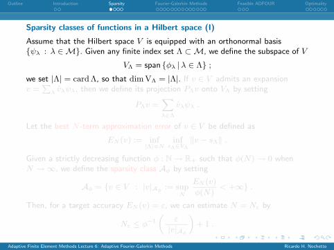
Sparsity classes of functions in a Hilbert space (I)
Assume that the Hilbert space V is equipped with an orthonormal basisψλ : λ ∈M. Given any finite index set Λ ⊂M, we define the subspace of V
VΛ = span φλ |λ ∈ Λ ;
we set |Λ| = cardΛ, so that dim VΛ = |Λ|. If v ∈ V admits an expansionv =
Pλ vλψλ, then we define its projection PΛv onto VΛ by setting
PΛv =Xλ∈Λ
vλψλ .
Let the best N -term approximation error of v ∈ V be defined as
EN (v) := inf|Λ|=N
infsΛ∈VΛ
‖v − sΛ‖ .
Given a strictly decreasing function φ : N → R+ such that φ(N) → 0 whenN →∞, we define the sparsity class Aφ by setting
Aφ = v ∈ V : |v|Aφ := supN
EN (v)
φ(N)< +∞ .
Then, for a target accuracy EN (v) = ε, we can estimate N = Nε by
Nε ≤ φ−1
„ε
|v|Aφ
«+ 1 .
Adaptive Finite Element Methods Lecture 6: Adaptive Fourier-Galerkin Methods Ricardo H. Nochetto

Outline Introduction Sparsity Fourier-Galerkin Methods Feasible ADFOUR Optimality
Sparsity classes of functions in a Hilbert space (I)
Assume that the Hilbert space V is equipped with an orthonormal basisψλ : λ ∈M. Given any finite index set Λ ⊂M, we define the subspace of V
VΛ = span φλ |λ ∈ Λ ;
we set |Λ| = cardΛ, so that dim VΛ = |Λ|. If v ∈ V admits an expansionv =
Pλ vλψλ, then we define its projection PΛv onto VΛ by setting
PΛv =Xλ∈Λ
vλψλ .
Let the best N -term approximation error of v ∈ V be defined as
EN (v) := inf|Λ|=N
infsΛ∈VΛ
‖v − sΛ‖ .
Given a strictly decreasing function φ : N → R+ such that φ(N) → 0 whenN →∞, we define the sparsity class Aφ by setting
Aφ = v ∈ V : |v|Aφ := supN
EN (v)
φ(N)< +∞ .
Then, for a target accuracy EN (v) = ε, we can estimate N = Nε by
Nε ≤ φ−1
„ε
|v|Aφ
«+ 1 .
Adaptive Finite Element Methods Lecture 6: Adaptive Fourier-Galerkin Methods Ricardo H. Nochetto
Outline Introduction Sparsity Fourier-Galerkin Methods Feasible ADFOUR Optimality
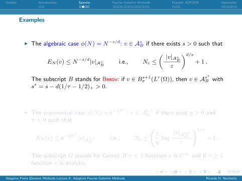
Examples
I The algebraic case φ(N) = N−s/d: v ∈ AsB if there exists s > 0 such that
EN (v) ≤ N−s/d|v|AsB
i.e., Nε ≤„ |v|As
B
ε
«d/s
+ 1 .
The subscript B stands for Besov: if v ∈ Bs+1σ (Lr(Ω)), then v ∈ As∗
B withs∗ = s− d(1/τ − 1/2)+ > 0.
I The exponential case φ(N) = e−ηNτ
: v ∈ Aη,τG if there exist η > 0 and
τ > 0 such that
EN (v) ≤ e−ηNτ
|v|Aη,τG
i.e., Nε ≤
1
ηlog
|v|Aη,τG
ε
!1/τ
+ 1 .
The subscript G stands for Gevrey. If τ < 1 function v is C∞ and if τ ≥ 1function v is analytic.
Adaptive Finite Element Methods Lecture 6: Adaptive Fourier-Galerkin Methods Ricardo H. Nochetto

Outline Introduction Sparsity Fourier-Galerkin Methods Feasible ADFOUR Optimality
Examples
I The algebraic case φ(N) = N−s/d: v ∈ AsB if there exists s > 0 such that
EN (v) ≤ N−s/d|v|AsB
i.e., Nε ≤„ |v|As
B
ε
«d/s
+ 1 .
The subscript B stands for Besov: if v ∈ Bs+1σ (Lr(Ω)), then v ∈ As∗
B withs∗ = s− d(1/τ − 1/2)+ > 0.
I The exponential case φ(N) = e−ηNτ
: v ∈ Aη,τG if there exist η > 0 and
τ > 0 such that
EN (v) ≤ e−ηNτ
|v|Aη,τG
i.e., Nε ≤
1
ηlog
|v|Aη,τG
ε
!1/τ
+ 1 .
The subscript G stands for Gevrey. If τ < 1 function v is C∞ and if τ ≥ 1function v is analytic.
Adaptive Finite Element Methods Lecture 6: Adaptive Fourier-Galerkin Methods Ricardo H. Nochetto
Outline Introduction Sparsity Fourier-Galerkin Methods Feasible ADFOUR Optimality
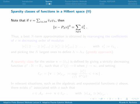
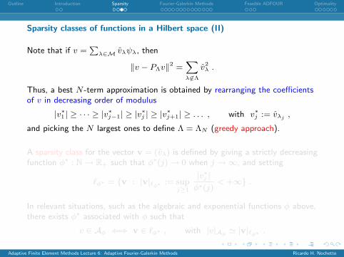
Sparsity classes of functions in a Hilbert space (II)
Note that if v =P
λ∈M vλψλ, then
‖v − PΛv‖2 =Xλ 6∈Λ
v2λ .
Thus, a best N -term approximation is obtained by rearranging the coefficientsof v in decreasing order of modulus
|v∗1 | ≥ · · · ≥ |v∗j−1| ≥ |v∗j | ≥ |v∗j+1| ≥ . . . , with v∗j := vλj ,
and picking the N largest ones to define Λ = ΛN (greedy approach).
A sparsity class for the vector v = (vλ) is defined by giving a strictly decreasingfunction φ∗ : N → R+ such that φ∗(j) → 0 when j →∞, and setting
`φ∗ = v : |v|`φ∗ := supj≥1
|v∗j |φ∗(j)
< +∞ .
In relevant situations, such as the algebraic and exponential functions φ above,there exists φ∗ associated with φ such that
v ∈ Aφ ⇐⇒ v ∈ `φ∗ , with |v|Aφ ' |v|`φ∗ .
Adaptive Finite Element Methods Lecture 6: Adaptive Fourier-Galerkin Methods Ricardo H. Nochetto
Outline Introduction Sparsity Fourier-Galerkin Methods Feasible ADFOUR Optimality
Sparsity classes of functions in a Hilbert space (II)
Note that if v =P
λ∈M vλψλ, then
‖v − PΛv‖2 =Xλ 6∈Λ
v2λ .
Thus, a best N -term approximation is obtained by rearranging the coefficientsof v in decreasing order of modulus
|v∗1 | ≥ · · · ≥ |v∗j−1| ≥ |v∗j | ≥ |v∗j+1| ≥ . . . , with v∗j := vλj ,
and picking the N largest ones to define Λ = ΛN (greedy approach).
A sparsity class for the vector v = (vλ) is defined by giving a strictly decreasingfunction φ∗ : N → R+ such that φ∗(j) → 0 when j →∞, and setting
`φ∗ = v : |v|`φ∗ := supj≥1
|v∗j |φ∗(j)
< +∞ .
In relevant situations, such as the algebraic and exponential functions φ above,there exists φ∗ associated with φ such that
v ∈ Aφ ⇐⇒ v ∈ `φ∗ , with |v|Aφ ' |v|`φ∗ .
Adaptive Finite Element Methods Lecture 6: Adaptive Fourier-Galerkin Methods Ricardo H. Nochetto

Outline Introduction Sparsity Fourier-Galerkin Methods Feasible ADFOUR Optimality
Explicit vs Implicit Knowledge of a Function
I If the function to be approximated is explicitly known through itsexpansion coefficients with respect to the chosen basis, then computing itsbest approximation (for a given cardinality N , or for a given accuracy ε)amounts to thresholding its rearranged coefficients.
I The situation is much harder if the function is only implicitly known as thesolution of an operator equation
Lu = f .
We may only assume to have full access to the data f and the operator L,and thereby to the residual r(uΛ) = f − LuΛ (or a truncated form of it),with uΛ the Galerkin solution over the discrete set Λ.
Adaptive Finite Element Methods Lecture 6: Adaptive Fourier-Galerkin Methods Ricardo H. Nochetto

Outline Introduction Sparsity Fourier-Galerkin Methods Feasible ADFOUR Optimality
Outline
Introduction
Sparsity
Adaptive Fourier-Galerkin Methods
F-ADFOUR: Feasible ADFOUR
Optimality of Adaptive Algorithms
Adaptive Finite Element Methods Lecture 6: Adaptive Fourier-Galerkin Methods Ricardo H. Nochetto

Outline Introduction Sparsity Fourier-Galerkin Methods Feasible ADFOUR Optimality
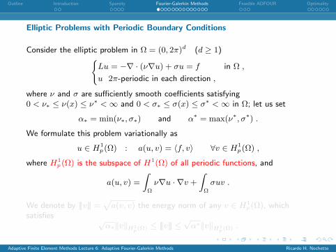
Elliptic Problems with Periodic Boundary Conditions
Consider the elliptic problem in Ω = (0, 2π)d (d ≥ 1)(Lu = −∇ · (ν∇u) + σu = f in Ω ,
u 2π-periodic in each direction ,
where ν and σ are sufficiently smooth coefficients satisfying0 < ν∗ ≤ ν(x) ≤ ν∗ <∞ and 0 < σ∗ ≤ σ(x) ≤ σ∗ <∞ in Ω; let us set
α∗ = min(ν∗, σ∗) and α∗ = max(ν∗, σ∗) .
We formulate this problem variationally as
u ∈ H1p(Ω) : a(u, v) = 〈f, v〉 ∀v ∈ H1
p(Ω) ,
where H1p(Ω) is the subspace of H1(Ω) of all periodic functions, and
a(u, v) =
ZΩ
ν∇u · ∇v +
ZΩ
σuv .
We denote by |||v||| =pa(v, v) the energy norm of any v ∈ H1
p(Ω), whichsatisfies √
α∗‖v‖H1p(Ω) ≤ |||v||| ≤
√α∗‖v‖H1
p(Ω) .
Adaptive Finite Element Methods Lecture 6: Adaptive Fourier-Galerkin Methods Ricardo H. Nochetto
Outline Introduction Sparsity Fourier-Galerkin Methods Feasible ADFOUR Optimality
Elliptic Problems with Periodic Boundary Conditions
Consider the elliptic problem in Ω = (0, 2π)d (d ≥ 1)(Lu = −∇ · (ν∇u) + σu = f in Ω ,
u 2π-periodic in each direction ,
where ν and σ are sufficiently smooth coefficients satisfying0 < ν∗ ≤ ν(x) ≤ ν∗ <∞ and 0 < σ∗ ≤ σ(x) ≤ σ∗ <∞ in Ω; let us set
α∗ = min(ν∗, σ∗) and α∗ = max(ν∗, σ∗) .
We formulate this problem variationally as
u ∈ H1p(Ω) : a(u, v) = 〈f, v〉 ∀v ∈ H1
p(Ω) ,
where H1p(Ω) is the subspace of H1(Ω) of all periodic functions, and
a(u, v) =
ZΩ
ν∇u · ∇v +
ZΩ
σuv .
We denote by |||v||| =pa(v, v) the energy norm of any v ∈ H1
p(Ω), whichsatisfies √
α∗‖v‖H1p(Ω) ≤ |||v||| ≤
√α∗‖v‖H1
p(Ω) .
Adaptive Finite Element Methods Lecture 6: Adaptive Fourier-Galerkin Methods Ricardo H. Nochetto

Outline Introduction Sparsity Fourier-Galerkin Methods Feasible ADFOUR Optimality
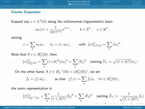
Fourier Expansion
Expand any v ∈ L2(Ω) along the orthonormal trigonometric basis
φk(x) =1
(2π)d/2eik·x , k ∈ Zd , x ∈ Rd ,
setting
v =X
k
vkφk , vk = (v, φk) , with ‖v‖2L2(Ω) =X
k
|vk|2 .
Note that if v ∈ H1p(Ω), then
‖v‖2 =‖v‖2H1p(Ω) =
Xk
(1+|k|2)|vk|2 =X
k
|Vk|2 (setting Vk :=p
(1 + |k|2)vk) .
On the other hand, if f ∈ H−1p (Ω) = (H1
p(Ω))′, we set
fk = 〈f, φk〉 , so that 〈f, v〉 =X
k
fkvk ∀v ∈ H1p(Ω) ;
the norm representation is
‖f‖2 =‖f‖2H−1
p (Ω)=X
k
1
(1 + |k|2) |fk|2 =X
k
|Fk|2 (setting Fk :=1p
(1 + |k|2)fk) .
Adaptive Finite Element Methods Lecture 6: Adaptive Fourier-Galerkin Methods Ricardo H. Nochetto

Outline Introduction Sparsity Fourier-Galerkin Methods Feasible ADFOUR Optimality
Fourier Expansion
Expand any v ∈ L2(Ω) along the orthonormal trigonometric basis
φk(x) =1
(2π)d/2eik·x , k ∈ Zd , x ∈ Rd ,
setting
v =X
k
vkφk , vk = (v, φk) , with ‖v‖2L2(Ω) =X
k
|vk|2 .
Note that if v ∈ H1p(Ω), then
‖v‖2 =‖v‖2H1p(Ω) =
Xk
(1+|k|2)|vk|2 =X
k
|Vk|2 (setting Vk :=p
(1 + |k|2)vk) .
On the other hand, if f ∈ H−1p (Ω) = (H1
p(Ω))′, we set
fk = 〈f, φk〉 , so that 〈f, v〉 =X
k
fkvk ∀v ∈ H1p(Ω) ;
the norm representation is
‖f‖2 =‖f‖2H−1
p (Ω)=X
k
1
(1 + |k|2) |fk|2 =X
k
|Fk|2 (setting Fk :=1p
(1 + |k|2)fk) .
Adaptive Finite Element Methods Lecture 6: Adaptive Fourier-Galerkin Methods Ricardo H. Nochetto
Outline Introduction Sparsity Fourier-Galerkin Methods Feasible ADFOUR Optimality
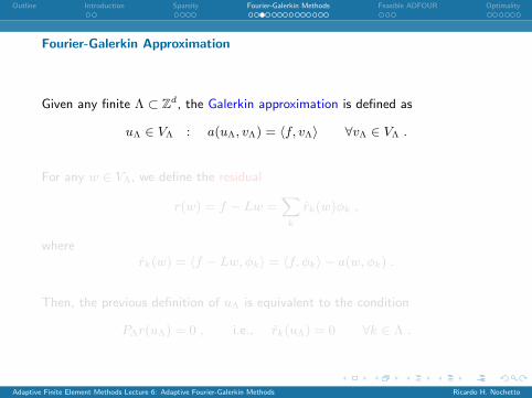
Fourier-Galerkin Approximation
Given any finite Λ ⊂ Zd, the Galerkin approximation is defined as
uΛ ∈ VΛ : a(uΛ, vΛ) = 〈f, vΛ〉 ∀vΛ ∈ VΛ .
For any w ∈ VΛ, we define the residual
r(w) = f − Lw =X
k
rk(w)φk ,
whererk(w) = 〈f − Lw, φk〉 = 〈f, φk〉 − a(w, φk) .
Then, the previous definition of uΛ is equivalent to the condition
PΛr(uΛ) = 0 , i.e., rk(uΛ) = 0 ∀k ∈ Λ .
Adaptive Finite Element Methods Lecture 6: Adaptive Fourier-Galerkin Methods Ricardo H. Nochetto

Outline Introduction Sparsity Fourier-Galerkin Methods Feasible ADFOUR Optimality
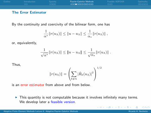
The Error Estimator
By the continuity and coercivity of the bilinear form, one has
1
α∗‖r(uΛ)‖ ≤ ‖u− uΛ‖ ≤
1
α∗‖r(uΛ)‖ ,
or, equivalently,
1√α∗‖r(uΛ)‖ ≤ |||u− uΛ||| ≤
1√α∗‖r(uΛ)‖ .
Thus,
‖r(uΛ)‖ =
0@Xk 6∈Λ
|Rk(uΛ)|21A1/2
is an error estimator from above and from below.
I This quantity is not computable because it involves infinitely many terms.We develop later a feasible version.
Adaptive Finite Element Methods Lecture 6: Adaptive Fourier-Galerkin Methods Ricardo H. Nochetto

Outline Introduction Sparsity Fourier-Galerkin Methods Feasible ADFOUR Optimality
The Error Estimator
By the continuity and coercivity of the bilinear form, one has
1
α∗‖r(uΛ)‖ ≤ ‖u− uΛ‖ ≤
1
α∗‖r(uΛ)‖ ,
or, equivalently,
1√α∗‖r(uΛ)‖ ≤ |||u− uΛ||| ≤
1√α∗‖r(uΛ)‖ .
Thus,
‖r(uΛ)‖ =
0@Xk 6∈Λ
|Rk(uΛ)|21A1/2
is an error estimator from above and from below.
I This quantity is not computable because it involves infinitely many terms.We develop later a feasible version.
Adaptive Finite Element Methods Lecture 6: Adaptive Fourier-Galerkin Methods Ricardo H. Nochetto

Outline Introduction Sparsity Fourier-Galerkin Methods Feasible ADFOUR Optimality
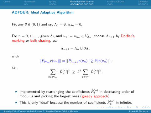
ADFOUR: Ideal Adaptive Algorithm
Fix any θ ∈ (0, 1) and set Λ0 = ∅, uΛ0 = 0.
For n = 0, 1, . . . , given Λn and un := uΛn ∈ VΛn , choose Λn+1 by Dorfler’smarking or bulk chasing, as:
Λn+1 = Λn ∪ ∂Λn
with‖P∂Λnr(un)‖ = ‖PΛn+1r(un)‖ ≥ θ‖r(un)‖ ,
i.e., Xk∈∂Λn
|R(n)k |2 ≥ θ2
Xk∈Zd
|R(n)k |2 .
I Implemented by rearranging the coefficients R(n)k in decreasing order of
modulus and picking the largest ones (greedy approach).
I This is only ’ideal’ because the number of coefficients R(n)k in infinite.
Adaptive Finite Element Methods Lecture 6: Adaptive Fourier-Galerkin Methods Ricardo H. Nochetto
Outline Introduction Sparsity Fourier-Galerkin Methods Feasible ADFOUR Optimality
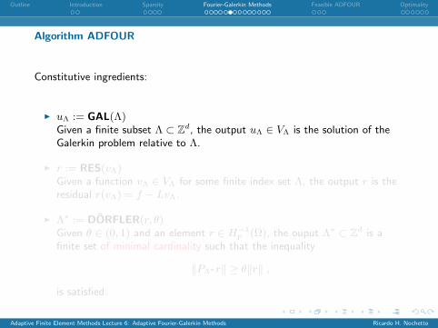
Algorithm ADFOUR
Constitutive ingredients:
I uΛ := GAL(Λ)Given a finite subset Λ ⊂ Zd, the output uΛ ∈ VΛ is the solution of theGalerkin problem relative to Λ.
I r := RES(vΛ)Given a function vΛ ∈ VΛ for some finite index set Λ, the output r is theresidual r(vΛ) = f − LvΛ.
I Λ∗ := DORFLER(r, θ)Given θ ∈ (0, 1) and an element r ∈ H−1
p (Ω), the ouput Λ∗ ⊂ Zd is afinite set of minimal cardinality such that the inequality
‖PΛ∗r‖ ≥ θ‖r‖ ,
is satisfied.
Adaptive Finite Element Methods Lecture 6: Adaptive Fourier-Galerkin Methods Ricardo H. Nochetto

Outline Introduction Sparsity Fourier-Galerkin Methods Feasible ADFOUR Optimality
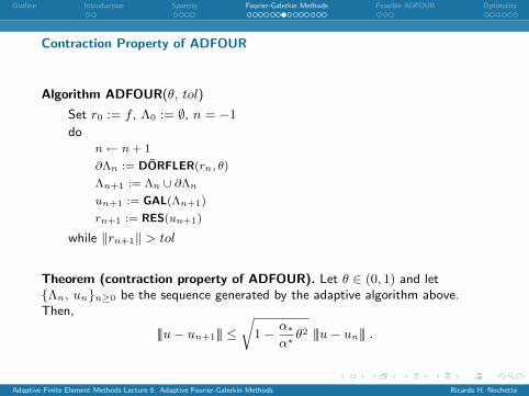
Contraction Property of ADFOUR
Algorithm ADFOUR(θ, tol)
Set r0 := f , Λ0 := ∅, n = −1
don← n + 1
∂Λn := DORFLER(rn, θ)
Λn+1 := Λn ∪ ∂Λn
un+1 := GAL(Λn+1)
rn+1 := RES(un+1)
while ‖rn+1‖ > tol
Theorem (contraction property of ADFOUR). Let θ ∈ (0, 1) and letΛn, unn≥0 be the sequence generated by the adaptive algorithm above.Then,
|||u− un+1||| ≤r
1− α∗α∗θ2 |||u− un||| .
Adaptive Finite Element Methods Lecture 6: Adaptive Fourier-Galerkin Methods Ricardo H. Nochetto
Outline Introduction Sparsity Fourier-Galerkin Methods Feasible ADFOUR Optimality
Contraction Property of ADFOUR
Algorithm ADFOUR(θ, tol)
Set r0 := f , Λ0 := ∅, n = −1
don← n + 1
∂Λn := DORFLER(rn, θ)
Λn+1 := Λn ∪ ∂Λn
un+1 := GAL(Λn+1)
rn+1 := RES(un+1)
while ‖rn+1‖ > tol
Theorem (contraction property of ADFOUR). Let θ ∈ (0, 1) and letΛn, unn≥0 be the sequence generated by the adaptive algorithm above.Then,
|||u− un+1||| ≤r
1− α∗α∗θ2 |||u− un||| .
Adaptive Finite Element Methods Lecture 6: Adaptive Fourier-Galerkin Methods Ricardo H. Nochetto

Outline Introduction Sparsity Fourier-Galerkin Methods Feasible ADFOUR Optimality
Proof of the Contraction Property
We use the notation en := |||u− un||| and dn := |||un+1 − un|||.
As VΛn ⊂ VΛn+1 , the following Galerkin orthogonality property holds
e2n+1 = e2n − d2n.
On the other hand, for any w ∈ H1p(Ω), one has
‖Lw‖ ≤√α∗ |||w||| .
Thus,
d2n ≥ 1
α∗‖L(un+1 − un)‖2 =
1
α∗‖rn+1 − rn‖2
≥ 1
α∗‖PΛn+1(rn+1 − rn)‖2 =
1
α∗‖PΛn+1rn‖2 ≥
θ2
α∗‖rn‖2 .
We conclude by recalling that
‖rn‖2 ≥ α∗e2n .
Adaptive Finite Element Methods Lecture 6: Adaptive Fourier-Galerkin Methods Ricardo H. Nochetto

Outline Introduction Sparsity Fourier-Galerkin Methods Feasible ADFOUR Optimality
Aggressive Version of ADFOUR: Motivation
The contraction factor guaranteed for ADFOUR is bounded from below awayof 0:
ρ = ρ(θ) =
r1− α∗
α∗θ2 ≥
r1− α∗
α∗> 0 .
Such a result is overly pessimistic, particularly in the case of smooth (analytic)solutions, since a Fourier method allows for an exponential decay of the error asthe number of (properly selected) active degrees of freedom is increased.
0 10 20 30 40 50 60 70−14
−12
−10
−8
−6
−4
−2
0
2
Energy error vs number of activated degrees of freedom
I black curve:θ2 = .9
I blue curve:θ2 = .999
I red curve:θ2 = .99999
Adaptive Finite Element Methods Lecture 6: Adaptive Fourier-Galerkin Methods Ricardo H. Nochetto
Outline Introduction Sparsity Fourier-Galerkin Methods Feasible ADFOUR Optimality
Aggressive Version of ADFOUR: Enrichment of the Active Set
The “quasi-diagonal” structure of the operator L in Fourier space suggests animprovement of the strategy.
The “stiffness” matrix A representing the operator Lu = −∇ · (ν∇u) + σuwith respect to the Fourier basis has elements
ak,m =1p
(1 + |k|2)(1 + |m|2)(k ·m νk−m + σk−m) .
Thus, if the operator coefficients ν and σ are analytic, their Fourier coefficientsdecay exponentially, hence there exist positive constants cL and ηL such that
|ak,m| ≤ cLexp(−ηL|k −m|) as |k −m| → ∞ .
This property implies that a “small” enrichment of the set of the newly addeddegrees of freedom may yield a “big” gain in accuracy. This motivates the new2-step procedure f∂Λn :=DORFLER(rn, θ)
∂Λn :=ENRICH(f∂Λn, θ) .
Adaptive Finite Element Methods Lecture 6: Adaptive Fourier-Galerkin Methods Ricardo H. Nochetto

Outline Introduction Sparsity Fourier-Galerkin Methods Feasible ADFOUR Optimality
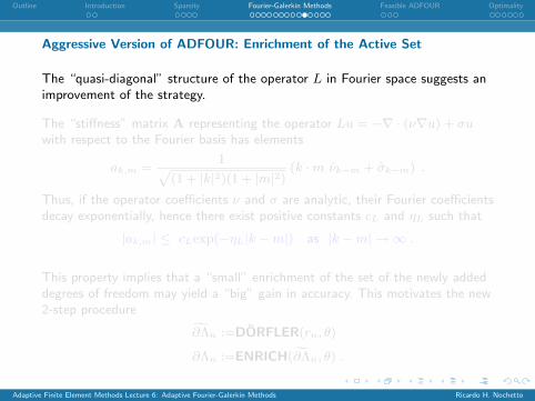
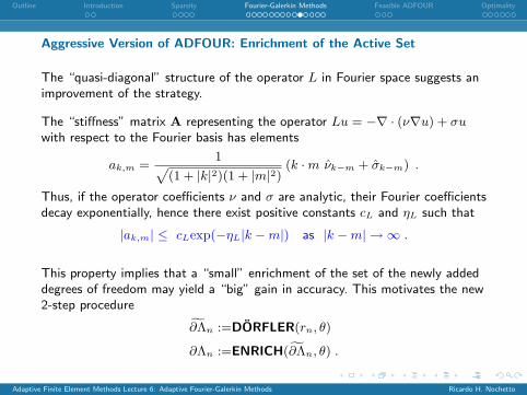
Aggressive Version of ADFOUR: Enrichment of the Active Set
The “quasi-diagonal” structure of the operator L in Fourier space suggests animprovement of the strategy.
The “stiffness” matrix A representing the operator Lu = −∇ · (ν∇u) + σuwith respect to the Fourier basis has elements
ak,m =1p
(1 + |k|2)(1 + |m|2)(k ·m νk−m + σk−m) .
Thus, if the operator coefficients ν and σ are analytic, their Fourier coefficientsdecay exponentially, hence there exist positive constants cL and ηL such that
|ak,m| ≤ cLexp(−ηL|k −m|) as |k −m| → ∞ .
This property implies that a “small” enrichment of the set of the newly addeddegrees of freedom may yield a “big” gain in accuracy. This motivates the new2-step procedure f∂Λn :=DORFLER(rn, θ)
∂Λn :=ENRICH(f∂Λn, θ) .
Adaptive Finite Element Methods Lecture 6: Adaptive Fourier-Galerkin Methods Ricardo H. Nochetto
Outline Introduction Sparsity Fourier-Galerkin Methods Feasible ADFOUR Optimality
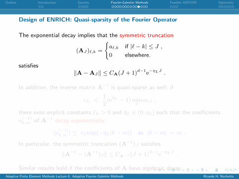
Design of ENRICH: Quasi-sparsity of the Fourier Operator
The exponential decay implies that the symmetric truncation
(AJ)`,k =
(a`,k if |`− k| ≤ J ,
0 elsewhere.
satisfies‖A−AJ‖ ≤ CA(J + 1)d−1e−ηLJ .
In addition, the inverse matrix A−1 is quasi-sparse as well: if
cL <1
2(eηL − 1)min
`a`,` ,
there exist explicit constants cL > 0 and ηL ∈ (0, ηL] such that the coefficients
a(−1)k,m of A−1 decay exponentially:
|a(−1)k,m | ≤ cLexp(−ηL|k −m|) as |k −m| → ∞ .
In particular, the symmetric truncation (A−1)J satisfies
‖A−1 − (A−1)J‖ ≤ CA−1(J + 1)d−1e−ηLJ .
Similar results hold if the coefficients of A have algebraic decay.Adaptive Finite Element Methods Lecture 6: Adaptive Fourier-Galerkin Methods Ricardo H. Nochetto

Outline Introduction Sparsity Fourier-Galerkin Methods Feasible ADFOUR Optimality
Design of ENRICH (continued)
We define the new active set Λn+1 := Λn ∪ ∂Λn by the 2-step procedure:f∂Λn :=DORFLER(rn, θ)
∂Λn :=ENRICH(f∂Λn, J)
To choose ∂Λn we note that gn = Pf∂Λnrn satisfies
‖rn − gn‖ ≤p
1− θ2‖rn‖.
Write wn = L−1gn ∈ V and decompose it as
wn = PΛn+1wn + PΛcn+1
wn = yn + zn ∈ VΛn+1 ⊕ VΛcn+1
Then, since zn =`PΛc
n+1L−1Pf∂Λn
´rn we see that
|||u− un+1||| ≤ |||u− (un + yn)||| ≤ 1√α∗‖L(u− un − wn‖+
√α∗‖zn‖
≤ 1√α∗
p1− θ2‖rn‖+
√α∗‖
`PΛc
n+1L−1Pf∂Λn
´rn‖ .
Conclusion: The construction of ∂Λn hinges on the operator PΛcn+1
L−1Pf∂Λn.
Adaptive Finite Element Methods Lecture 6: Adaptive Fourier-Galerkin Methods Ricardo H. Nochetto

Outline Introduction Sparsity Fourier-Galerkin Methods Feasible ADFOUR Optimality
Design of ENRICH (continued)
If ∂Λn is defined in such a way that
k ∈ Λcn+1 and ` ∈ f∂Λn ⇒ |k − `| > J ,
we have
‖PΛcn+1
L−1P∂Λn‖ ≤ ‖A−1 − (A−1)J‖ ≤ CA−1(J + 1)d−1e−ηLJ .
If J = J(θ) satisfies
CA−1(J + 1)d−1e−ηLJ ≤r
1− θ2
α∗α∗,
then
|||u− un+1||| ≤rα∗
α∗
p1− θ2 |||u− un||| .
The procedure Λ∗ := ENRICH(Λ, J) is thus defined as follows: Given aninteger J ≥ 0 and a finite set Λ ⊂ Zd, the output is the set
Λ∗ := k ∈ Zd : there exists ` ∈ Λ such that |k − `| ≤ J .
Adaptive Finite Element Methods Lecture 6: Adaptive Fourier-Galerkin Methods Ricardo H. Nochetto
Outline Introduction Sparsity Fourier-Galerkin Methods Feasible ADFOUR Optimality
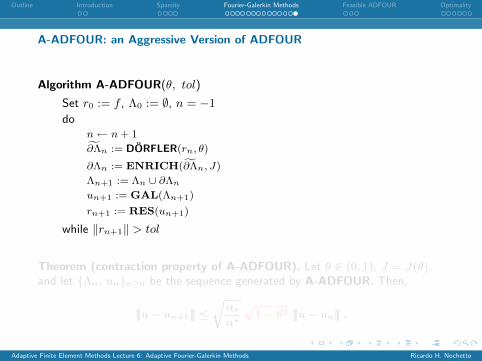
A-ADFOUR: an Aggressive Version of ADFOUR
Algorithm A-ADFOUR(θ, tol)
Set r0 := f , Λ0 := ∅, n = −1
don← n + 1f∂Λn := DORFLER(rn, θ)
∂Λn := ENRICH(f∂Λn, J)
Λn+1 := Λn ∪ ∂Λn
un+1 := GAL(Λn+1)
rn+1 := RES(un+1)
while ‖rn+1‖ > tol
Theorem (contraction property of A-ADFOUR). Let θ ∈ (0, 1), J = J(θ),and let Λn, unn≥0 be the sequence generated by A-ADFOUR. Then,
|||u− un+1||| ≤rα∗α∗
p1− θ2 |||u− un||| .
Adaptive Finite Element Methods Lecture 6: Adaptive Fourier-Galerkin Methods Ricardo H. Nochetto

Outline Introduction Sparsity Fourier-Galerkin Methods Feasible ADFOUR Optimality
Outline
Introduction
Sparsity
Adaptive Fourier-Galerkin Methods
F-ADFOUR: Feasible ADFOUR
Optimality of Adaptive Algorithms
Adaptive Finite Element Methods Lecture 6: Adaptive Fourier-Galerkin Methods Ricardo H. Nochetto

Outline Introduction Sparsity Fourier-Galerkin Methods Feasible ADFOUR Optimality
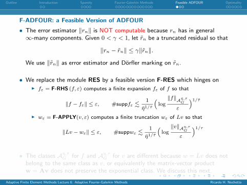
F-ADFOUR: a Feasible Version of ADFOUR
• The error estimator ‖rn‖ is NOT computable because rn has in general∞-many components. Given 0 < γ < 1, let rn be a truncated residual so that
‖rn − rn‖ ≤ γ‖rn‖.
We use ‖rn‖ as error estimator and Dorfler marking on rn.
• We replace the module RES by a feasible version F-RES which hinges onI fε = F-RHS (f, ε) computes a finite expansion fε of f so that
‖f − fε‖ ≤ ε, #suppfε .1
η1/τ
“log‖f‖Aη,τ
G
ε
”1/τ
I wε = F-APPLY(v, ε) computes a finite truncation wε of Lv so that
‖Lv − wε‖ ≤ ε, #suppwε .1
η1/τ
“log‖v‖Aη,τ
G
ε
”1/τ
• The classes Aη,τG for f and Aη,τ
G for v are different because w = Lv does notbelong to the same class as v, or equivalently the matrix-vector productw = Av does not preserve the exponential class. We discuss this next.
Adaptive Finite Element Methods Lecture 6: Adaptive Fourier-Galerkin Methods Ricardo H. Nochetto
Outline Introduction Sparsity Fourier-Galerkin Methods Feasible ADFOUR Optimality
F-ADFOUR: a Feasible Version of ADFOUR
• The error estimator ‖rn‖ is NOT computable because rn has in general∞-many components. Given 0 < γ < 1, let rn be a truncated residual so that
‖rn − rn‖ ≤ γ‖rn‖.
We use ‖rn‖ as error estimator and Dorfler marking on rn.
• We replace the module RES by a feasible version F-RES which hinges onI fε = F-RHS (f, ε) computes a finite expansion fε of f so that
‖f − fε‖ ≤ ε, #suppfε .1
η1/τ
“log‖f‖Aη,τ
G
ε
”1/τ
I wε = F-APPLY(v, ε) computes a finite truncation wε of Lv so that
‖Lv − wε‖ ≤ ε, #suppwε .1
η1/τ
“log‖v‖Aη,τ
G
ε
”1/τ
• The classes Aη,τG for f and Aη,τ
G for v are different because w = Lv does notbelong to the same class as v, or equivalently the matrix-vector productw = Av does not preserve the exponential class. We discuss this next.
Adaptive Finite Element Methods Lecture 6: Adaptive Fourier-Galerkin Methods Ricardo H. Nochetto

Outline Introduction Sparsity Fourier-Galerkin Methods Feasible ADFOUR Optimality
F-ADFOUR: a Feasible Version of ADFOUR (continued)
Algorithm F-ADFOUR(θ, γ, tol)
Set r0 := f , Λ0 := ∅, n = −1
r0 = F-RES(r0)
don← n + 1
∂Λn := DORFLER(rn, θ)
Λn+1 := Λn ∪ ∂Λn
un+1 := GAL(Λn+1)
rn+1 := F-RES(un+1, γ)
while ‖rn+1‖ > tol1+γ
Theorem (contraction property of F-ADFOUR). Let θ ∈ (0, 1), 0 < γ < θand let Λn, unn≥0 be the sequence generated by F-ADFOUR. Then,
|||u− un+1||| ≤r
1− α∗α∗θ2 |||u− un||| ,
with θ = θ−γ1+γ
.
Adaptive Finite Element Methods Lecture 6: Adaptive Fourier-Galerkin Methods Ricardo H. Nochetto
Outline Introduction Sparsity Fourier-Galerkin Methods Feasible ADFOUR Optimality
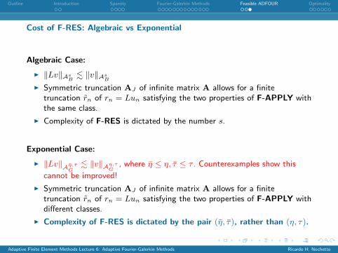
Cost of F-RES: Algebraic vs Exponential
Algebraic Case:
I ‖Lv‖AsB
. ‖v‖AsB
I Symmetric truncation AJ of infinite matrix A allows for a finitetruncation rn of rn = Lun satisfying the two properties of F-APPLY withthe same class.
I Complexity of F-RES is dictated by the number s.
Exponential Case:
I ‖Lv‖Aη,τG
. ‖v‖Aη,τG
, where η ≤ η, τ ≤ τ . Counterexamples show this
cannot be improved!
I Symmetric truncation AJ of infinite matrix A allows for a finitetruncation rn of rn = Lun satisfying the two properties of F-APPLY withdifferent classes.
I Complexity of F-RES is dictated by the pair (η, τ), rather than (η, τ).
Adaptive Finite Element Methods Lecture 6: Adaptive Fourier-Galerkin Methods Ricardo H. Nochetto

Outline Introduction Sparsity Fourier-Galerkin Methods Feasible ADFOUR Optimality
Outline
Introduction
Sparsity
Adaptive Fourier-Galerkin Methods
F-ADFOUR: Feasible ADFOUR
Optimality of Adaptive Algorithms
Adaptive Finite Element Methods Lecture 6: Adaptive Fourier-Galerkin Methods Ricardo H. Nochetto
Outline Introduction Sparsity Fourier-Galerkin Methods Feasible ADFOUR Optimality
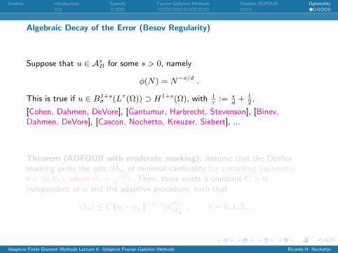
Algebraic Decay of the Error (Besov Regularity)
Suppose that u ∈ AsB for some s > 0, namely
φ(N) = N−s/d .
This is true if u ∈ B1+sσ (Lτ (Ω)) ⊃ H1+s(Ω), with 1
τ:= s
d+ 1
2.
[Cohen, Dahmen, DeVore], [Gantumur, Harbrecht, Stevenson], [Binev,Dahmen, DeVore], [Cascon, Nochetto, Kreuzer, Siebert], ...
Theorem (ADFOUR with moderate marking). Assume that the Dorflermarking picks the sets ∂Λn of minimal cardinality for a marking parameterθ ∈ (0, θ∗), where θ∗ =
pα∗α∗ . Then, there exists a constant C > 0
independent of u and the adaptive procedure, such that
|Λn| ≤ C|||u− un|||−d/s|u|d/sAs
B, n = 0, 1, 2, . . .
Adaptive Finite Element Methods Lecture 6: Adaptive Fourier-Galerkin Methods Ricardo H. Nochetto

Outline Introduction Sparsity Fourier-Galerkin Methods Feasible ADFOUR Optimality
Proof of Theorem
This is based on the following property [Stevenson], which exploits that Dorflermarking gives a minimal set: let µθ = 1− α∗
α∗θ2 > 0 and ε2n = µθ|||u− un|||2.
Then, |∂Λn| can be compared with the best set |Λεn(u)| for accuracy εn:
|∂Λn| ≤ |Λεn(u)| ≤ ε−d/sn |u|d/s
AsB, n = 0, 1, 2, . . .
The estimate for |Λn| then follows from
|∂Λm| <∼ |||u− um|||−d/s|u|d/sAs
B, m = 0, 1, 2, . . . , n− 1
and the decay rate stated in the Contraction Theorem
|||u− un||| ≤ ρn−m|||u− um||| , with ρ =“1− α∗
α∗θ”1/2
,
i.e.,|||u− um|||−1 ≤ ρm−n|||u− un|||−1 ,
via a geometric series argument:
|Λn| =n−1Xm=0
|∂Λm| <∼ |||u− un|||−d/s|u|d/sAs
B
n−1Xm=0
ρm <∼ |||u− un|||−d/s|u|d/sAs
B.
Adaptive Finite Element Methods Lecture 6: Adaptive Fourier-Galerkin Methods Ricardo H. Nochetto
Outline Introduction Sparsity Fourier-Galerkin Methods Feasible ADFOUR Optimality
Optimality of Aggressive ADFOUR: A-ADFOUR
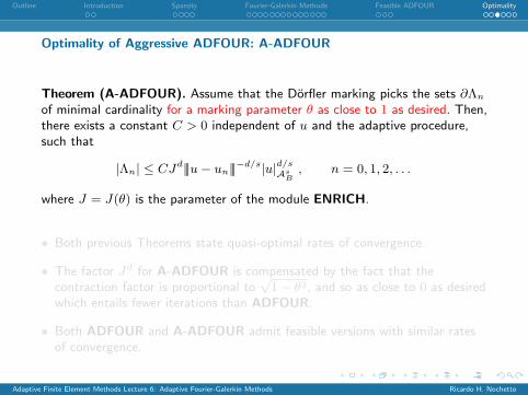
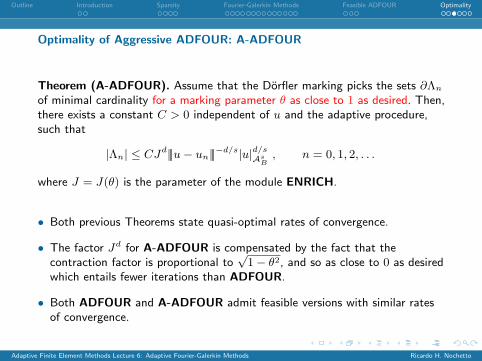
Theorem (A-ADFOUR). Assume that the Dorfler marking picks the sets ∂Λn
of minimal cardinality for a marking parameter θ as close to 1 as desired. Then,there exists a constant C > 0 independent of u and the adaptive procedure,such that
|Λn| ≤ CJd|||u− un|||−d/s|u|d/sAs
B, n = 0, 1, 2, . . .
where J = J(θ) is the parameter of the module ENRICH.
• Both previous Theorems state quasi-optimal rates of convergence.
• The factor Jd for A-ADFOUR is compensated by the fact that thecontraction factor is proportional to
√1− θ2, and so as close to 0 as desired
which entails fewer iterations than ADFOUR.
• Both ADFOUR and A-ADFOUR admit feasible versions with similar ratesof convergence.
Adaptive Finite Element Methods Lecture 6: Adaptive Fourier-Galerkin Methods Ricardo H. Nochetto
Outline Introduction Sparsity Fourier-Galerkin Methods Feasible ADFOUR Optimality
Optimality of Aggressive ADFOUR: A-ADFOUR
Theorem (A-ADFOUR). Assume that the Dorfler marking picks the sets ∂Λn
of minimal cardinality for a marking parameter θ as close to 1 as desired. Then,there exists a constant C > 0 independent of u and the adaptive procedure,such that
|Λn| ≤ CJd|||u− un|||−d/s|u|d/sAs
B, n = 0, 1, 2, . . .
where J = J(θ) is the parameter of the module ENRICH.
• Both previous Theorems state quasi-optimal rates of convergence.
• The factor Jd for A-ADFOUR is compensated by the fact that thecontraction factor is proportional to
√1− θ2, and so as close to 0 as desired
which entails fewer iterations than ADFOUR.
• Both ADFOUR and A-ADFOUR admit feasible versions with similar ratesof convergence.
Adaptive Finite Element Methods Lecture 6: Adaptive Fourier-Galerkin Methods Ricardo H. Nochetto

Outline Introduction Sparsity Fourier-Galerkin Methods Feasible ADFOUR Optimality
Exponential Decay of the Error (Gevrey Spaces)
Since the procedure F-RES computes the truncated residual rn and requiresmore degrees of freedom than the approximate solution un, we resort to acoarsening step:
I Λ := COARSE(w, ε)Given u ∈ Aη,τ
G and a function w ∈ V , which is known to satisfy
‖u− w‖ ≤ ε ,
the output Λ is a set of minimal cardinality such that
‖w − PΛw‖ ≤ 2ε ,
and
|Λ| ≤ 1
η1/τ
“log
‖u‖Aη,τG
ε
”1/τ
+ 1.
I Implemented by rearranging the coefficients wk of w in decreasing order ofmodulus and picking the largest ones (greedy approach).
Adaptive Finite Element Methods Lecture 6: Adaptive Fourier-Galerkin Methods Ricardo H. Nochetto

Outline Introduction Sparsity Fourier-Galerkin Methods Feasible ADFOUR Optimality
FF-ADFOUR: Feasible and Fast Version of ADFOUR
Algorithm FF-ADFOUR(θ, tol)
Set r0 := f , Λ0 := ∅, n = 0r0 := F-RES (r0)do f∂Λn := DORFLER (rn, θ)c∂Λn := ENRICH(f∂Λn, θ)bΛn+1 := Λn ∪ c∂Λnbun+1 := GAL(bΛn)
Λn+1 := COARSE“bun+1, 2
α∗
√1− θ2‖rn‖
”un+1 := GAL(Λn+1)
rn+1 := F-RES(un+1)
n← n + 1
while ‖rn+1‖ > tol
Theorem (contraction property of FF-ADFOUR). Let θ ∈ (0, 1) be as closeto 1 as desired and let Λn, unn≥0 be the sequence generated byFF-ADFOUR. Then,
|||u− un+1||| ≤ 6α∗α∗
p1− θ2 |||u− un||| .
Adaptive Finite Element Methods Lecture 6: Adaptive Fourier-Galerkin Methods Ricardo H. Nochetto

Outline Introduction Sparsity Fourier-Galerkin Methods Feasible ADFOUR Optimality
FF-ADFOUR: Feasible and Fast Version of ADFOUR
Algorithm FF-ADFOUR(θ, tol)
Set r0 := f , Λ0 := ∅, n = 0r0 := F-RES (r0)do f∂Λn := DORFLER (rn, θ)c∂Λn := ENRICH(f∂Λn, θ)bΛn+1 := Λn ∪ c∂Λnbun+1 := GAL(bΛn)
Λn+1 := COARSE“bun+1, 2
α∗
√1− θ2‖rn‖
”un+1 := GAL(Λn+1)
rn+1 := F-RES(un+1)
n← n + 1
while ‖rn+1‖ > tol
Theorem (contraction property of FF-ADFOUR). Let θ ∈ (0, 1) be as closeto 1 as desired and let Λn, unn≥0 be the sequence generated byFF-ADFOUR. Then,
|||u− un+1||| ≤ 6α∗α∗
p1− θ2 |||u− un||| .
Adaptive Finite Element Methods Lecture 6: Adaptive Fourier-Galerkin Methods Ricardo H. Nochetto
Outline Introduction Sparsity Fourier-Galerkin Methods Feasible ADFOUR Optimality
Cardinality of FF-ADFOUR
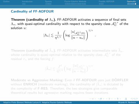
Theorem (cardinality of Λn). FF-ADFOUR activates a sequence of final setsΛn, with quasi-optimal cardinality with respect to the sparsity class Aη,τ
G of thesolution u:
|Λn| .1
η1/τ
log
|u|Aη,tG
(Ω)
‖u− un‖
!1/τ
.
Theorem (cardinality of bΛn). FF-ADFOUR activates intermediate sets bΛn,whose cardinality is quasi-optimal relative to the sparsity class Aη,τ
G of theresidual rn and the forcing f :
|bΛn| .Jd
η1/τ
“log
‖u‖Aη,τG
‖u− un‖
”1/τ
.
Moderate vs Aggressive Marking: Even if FF-ADFOUR uses just DORFLERwithout ENRICH (moderate marking), the cardinality of |bΛn| is dictated bythe complexity of F-RES. Therefore, the two strategies give comparabletheoretical results but agreessive marking requires fewer iterations.
Adaptive Finite Element Methods Lecture 6: Adaptive Fourier-Galerkin Methods Ricardo H. Nochetto

Outline Introduction Sparsity Fourier-Galerkin Methods Feasible ADFOUR Optimality
Cardinality of FF-ADFOUR
Theorem (cardinality of Λn). FF-ADFOUR activates a sequence of final setsΛn, with quasi-optimal cardinality with respect to the sparsity class Aη,τ
G of thesolution u:
|Λn| .1
η1/τ
log
|u|Aη,tG
(Ω)
‖u− un‖
!1/τ
.
Theorem (cardinality of bΛn). FF-ADFOUR activates intermediate sets bΛn,whose cardinality is quasi-optimal relative to the sparsity class Aη,τ
G of theresidual rn and the forcing f :
|bΛn| .Jd
η1/τ
“log
‖u‖Aη,τG
‖u− un‖
”1/τ
.
Moderate vs Aggressive Marking: Even if FF-ADFOUR uses just DORFLERwithout ENRICH (moderate marking), the cardinality of |bΛn| is dictated bythe complexity of F-RES. Therefore, the two strategies give comparabletheoretical results but agreessive marking requires fewer iterations.
Adaptive Finite Element Methods Lecture 6: Adaptive Fourier-Galerkin Methods Ricardo H. Nochetto