Adaptive dynamics for Articulated Bodies

Articulated Body dynamics

• Optimal forward dynamics algorithm– Linear time complexity– e.g. Featherstone’s DCA

algorithm– Not efficient enough for many

DoF systems

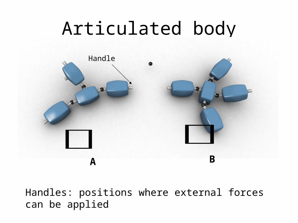
Articulated body

A B

Handles: positions where external forces can be applied

Handle

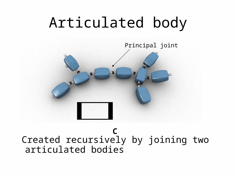
Articulated body

Created recursively by joining two articulated bodies

C

Principal joint

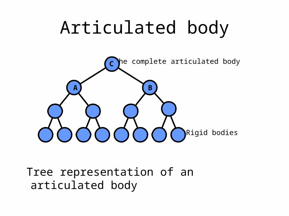
Articulated body

Tree representation of an articulated body

Rigid bodies

The complete articulated bodyC

A B

Featherstone’s DCA

• Articulated-body equation

• Change of in causes a change of in

BodyAccelerations

Inverse inertias and cross-inertias

AppliedForces

Biasaccelerations

jf jij fjf ia

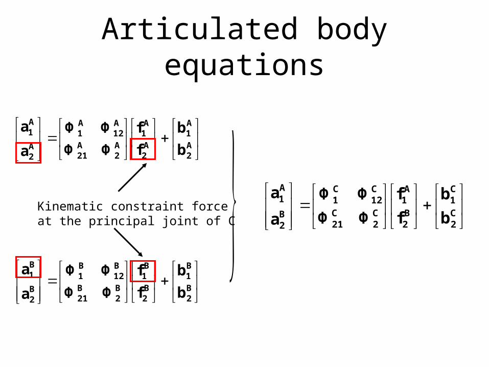
Articulated body equations

A2

A1

A2

A1

A2

A21

A12

A1

A2

A1

b

b

f

f

ΦΦ

ΦΦ

a

a

B2

B1

B2

B1

B2

B21

B12

B1

B2

B1

b

b

f

f

ΦΦ

ΦΦ

a

a

C2

C1

B2

A1

C2

C21

C12

C1

B2

A1

b

b

f

f

ΦΦ

ΦΦ

a

aKinematic constraint forceat the principal joint of C

Featherstone’s DCA Algorithm

• Update body velocity and position

• Main pass: Compute – Bottom-up pass

• Solve articulated body equation by back substitution– Top down pass

C2

C1

C12

C21

C2

C1 b,b,Φ,Φ,Φ,Φ

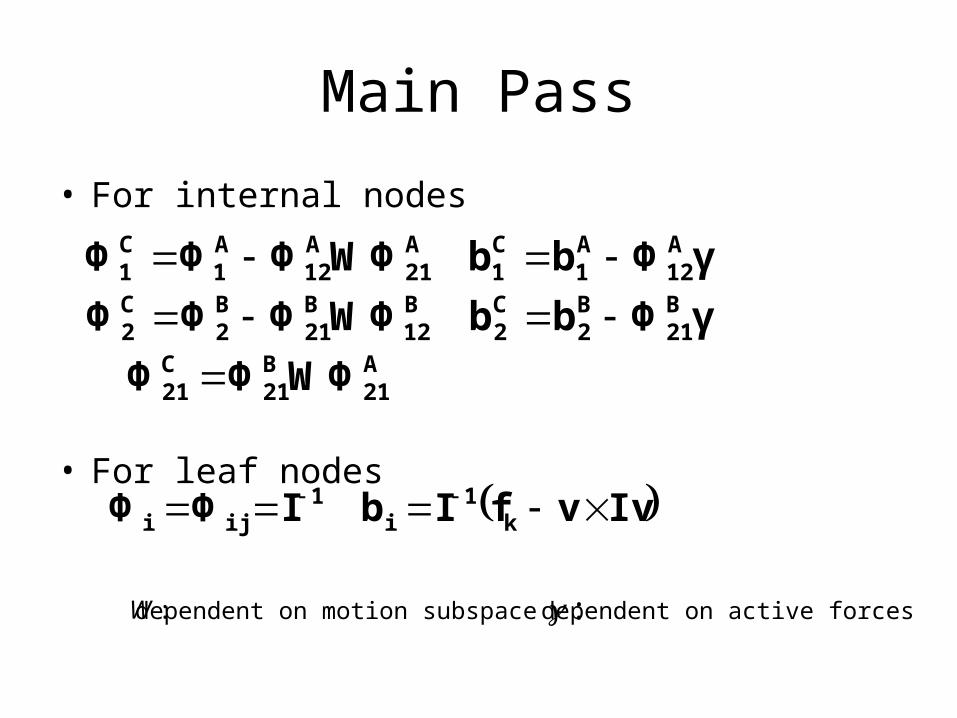
Main Pass

• For internal nodes

• For leaf nodes

IvvfIbIΦΦ k1

i1

iji

A21

B21

C21

B21

B2

C2

B12

B21

B2

C2

A12

A1

C1

A21

A12

A1

C1

WΦΦΦ

γΦbbWΦΦΦΦ

γΦbbWΦΦΦΦ

:W :dependent on motion subspace dependent on active forces

Back substitution

• Receive from parent

• Compute joint acceleration and using

• Send to A and to B

B2

A1 f,f

A2

B1 f,f

A2

A1 f,f

B2

B1 f,f

Adaptive Dynamics

• Simulate n most “important” joints

• Sacrifice amount of accuracy

• Other joints are rigidified

• “Important” and “accuracy” measures based on some motion metric

Hybrid body

Hybrid body

kf

Multilevel forward dynamics algorithm

• Compute body velocity and position only in active region

• Compute – Same as DCA for active nodes– Do not recompute for rigid nodes– (*) Compute in force update region using

• Back substitute only in active region

• Recompute hybrid body (at a different rate than the simulation timestep)

CC b,Φ

CΦCb

BA1BAAACi

C bbΦΦΦbbb

* For the metric we discuss later, this step is not performed

Motion metrics

• Acceleration metric

• Velocity metric

are SPD matrix i.e. metrics correspond to weighted sum of squaresii VA ,

• Theorem The acceleration metric value of an articulated body can be computed before computing its joint accelerations

Computing motion metric

Computing

• In active region compute using:

p,,

p,,

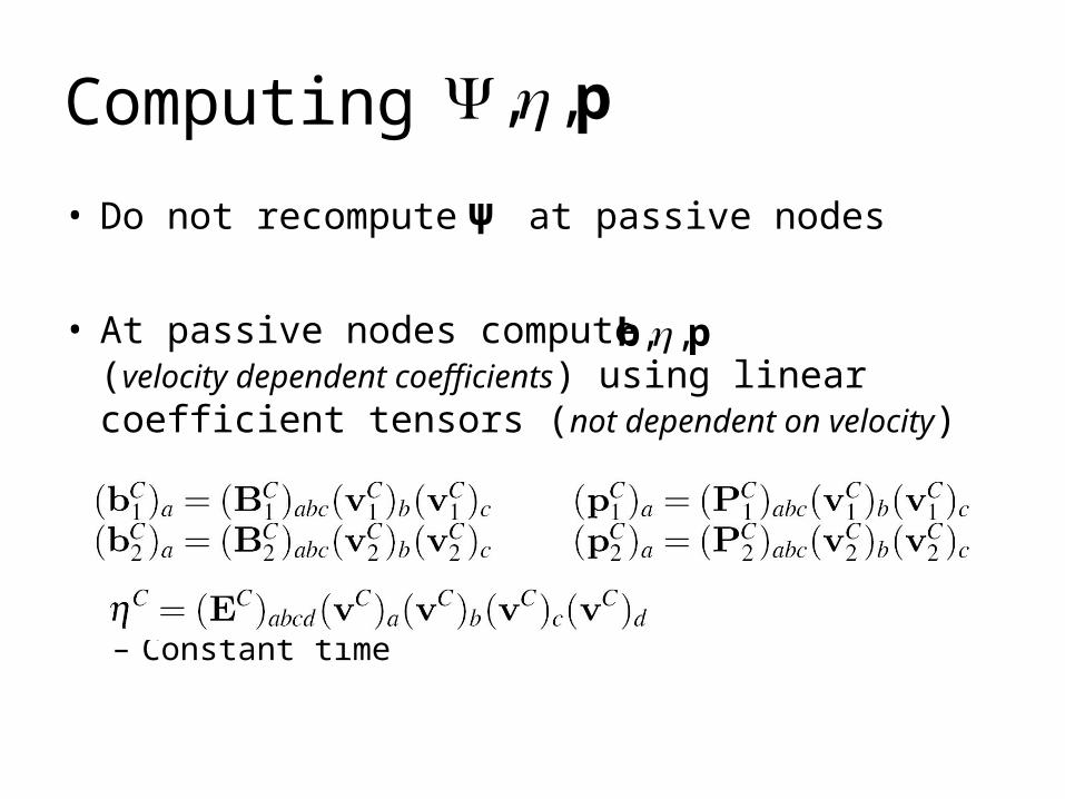
Computing

• Do not recompute at passive nodes

• At passive nodes compute (velocity

dependent coefficients) using linear coefficient tensors (not dependent on velocity)

– Constant time

p,,

pb ,,

Ψ

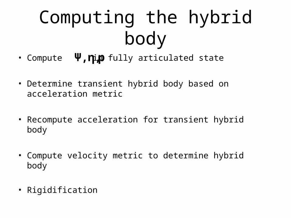
Computing the hybrid body

• Compute in fully articulated state

• Determine transient hybrid body based on acceleration metric

• Recompute acceleration for transient hybrid body

• Compute velocity metric to determine hybrid body

• Rigidification

pη,Ψ,

Adaptive joint selection Acceleration simplification

= 96

Compute the acceleration metric value of the root

= 96 -3

Compute the joint acceleration of the root

Adaptive joint selection Acceleration simplification

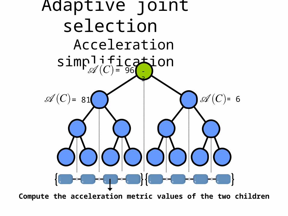
Adaptive joint selection Acceleration simplification

= 96

= 6 = 81

Compute the acceleration metric values of the two children

-3

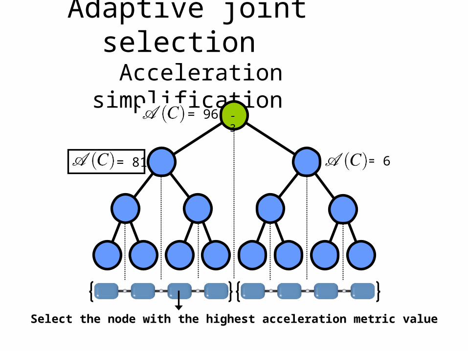
Adaptive joint selection Acceleration simplification

= 96

Select the node with the highest acceleration metric value

-3

= 6 = 81

Adaptive joint selection Acceleration simplification

= 96

Compute its joint acceleration

-3

-6 = 81 = 6

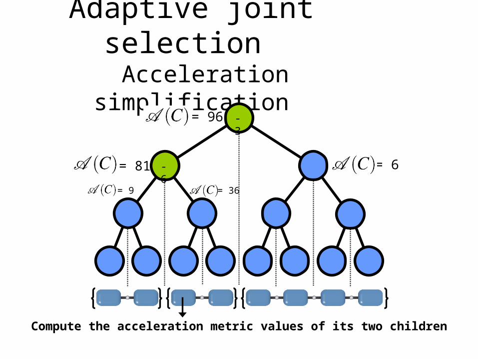
Adaptive joint selection Acceleration simplification

= 96

= 9 = 36

Compute the acceleration metric values of its two children

-3

-6 = 6 = 81

Adaptive joint selection Acceleration simplification

= 96

= 9 = 36

-3

-6 = 6 = 81

Select the node with the highest acceleration metric value

= 36

Adaptive joint selection Acceleration simplification

= 96

= 9 = 36

-3

-6 = 6 = 81

Compute its joint acceleration

6

Adaptive joint selection Acceleration simplification

-3

-6

6

Stop because a user-defined sufficient precision has been reached

= 96

= 9

= 6

Adaptive joint selection Acceleration simplification

-3

-6

6

Four subassemblies with joint accelerations implicitly set to zero

= 96

= 9

= 6

Velocity simplification

• Compute joint velocities in the transient active region (computed using acceleration metric)

• Compute metric in a bottom up manner from the transient rigid front using

• Compute rigid front like for acceleration metric

Rigidification

• Aim: Rigidify the joint velocities to 0

• Constraint:

• Solve for– Compute by computing– Compute

• Apply to the hybrid body

basis vector for

RR vΔv

KQΔvR QK jKe

R1ΔvKQ

Q

je Q

Rv

video

References

• FEATHERSTONE, R. 1999. A divide-and-conquer articulated body algorithm for parallel o(log(n)) calculation of rigid body dynamics. part 1: Basic

algorithm. International Journal of Robotics Research 18(9):867-875.

• S. Redon, N. Galoppo, and M. Lin. Adaptive dynamics of

articulated bodies: ACM Trans. on Graphics (Proc. of ACM SIGGRAPH), 24(3), 2005.