1 cs691 chow C. Edward Chow IDS: Intrusion Detection System.
Upload
clark-graggCategory
view
217download
1
Adaptive Design Methods in Clinical Trials
Shein-Chung Chow, PhD
Department of Biostatistics and BioinformaticsDuke University School of Medicine
Durham, North Carolina
Presented atThe 2011 MBSW, Muncie, Indiana
May 23, 2011

Lecture 1 - Outline
What is adaptive design? Type of adaptive designs
Possible benefits Regulatory perspectives Protocol amendments

What is adaptive design?
There is no universal definition. Adaptive randomization, group sequential,
and sample size re-estimation, etc. PhRMA (2006) FDA (2010)
Adaptive design is also known as Flexible design (EMEA, 2002, 2006) Attractive design (Uchida, 2006)

PhRMA’s definition
PhRMA (2006). J. Biopharm. Stat., 16 (3), 275-283.
An adaptive design is referred to as a clinical trial design that uses accumulating data to decide on how to modify aspects of the study as it continues, without undermining the validity and integrity of the trial.

PhRMA’s definition
Characteristics Adaptation is a design feature. Changes are made by design not
on an ad hoc basis. Comments
It does not reflect real practice. It may not be flexible as it means
to be.

FDA’s definition
US FDA Guidance for Industry – Adaptive Design Clinical Trials for Drugs and Biologics Feb, 2010
An adaptive design clinical study is defined as a study that includes a prospectively planned opportunity for modification of one or more specified aspects of the study design and hypotheses based on analysis of data (usually interim data) from subjects in the study

FDA’s definition Characteristics
Adaptation is a prospectively planned opportunity.
Changes are made based on analysis of data (usually interim data).
Does not include medical devices? Comments
It classifies adaptive designs into well-understood and less well-understood designs
It does not reflect real practice (protocol amendments)
It is not a guidance but a document of caution

Adaptation
An adaptation is defined as a change or modification made to a clinical trial before and during the conduct of the study.
Examples include Relax inclusion/exclusion criteria Change study endpoints Modify dose and treatment duration
etc.

Types of adaptations Prospective adaptations
Adaptive randomization Interim analysis Stopping trial early due to safety, futility, or efficacy Sample size re-estimation
etc. Concurrent adaptations
Trial procedures Implemented by protocol amendments
Retrospective adaptations Statistical procedures Implemented by statistical analysis plan prior to
database lock and/or data unblinding

Adaptive trial designs Adaptive randomization design Group sequential design Flexible sample size re-estimation design Drop-the-losers (play-the-winner) design Adaptive dose finding design Biomarker-adaptive design Adaptive treatment-switching design Adaptive-hypotheses design Seamless adaptive trial design Multiple adaptive design

Adaptive randomization design A design that allows modification of
randomization schedules Unequal probabilities of
treatment assignment Increase the probability of
success Types of adaptive randomization
Treatment-adaptive Covariate-adaptive Response-adaptive

Comments
Randomization schedule may not be available prior to the conduct of the study.
It may not be feasible for a large trial or a trial with a relatively long treatment duration.
Statistical inference on treatment effect is often difficult to obtain if it is not impossible.

Group sequential design
An adaptive design that allows for prematurely stopping a trial due to safety, efficacy/futility, or bothbased on interim analysis results
Sample size re-estimation Other adaptations
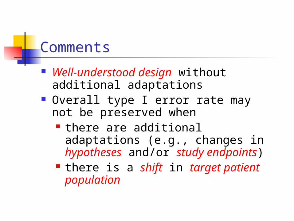
Comments Well-understood design without
additional adaptations Overall type I error rate may not be
preserved when there are additional adaptations
(e.g., changes in hypotheses and/or study endpoints)
there is a shift in target patient population

Flexible sample size re-estimation An adaptive design that allows for
sample size adjustment or re-estimation based on the observed data at interim blinding or unblinding
Sample size adjustment or re-estimation is usually performed based on the following criteria variability conditional power reproducibility probability
etc.

Comments
Can we always start with a small number and perform sample size re-estimation at interim?
It should be noted sample size re-estimation is performed based on estimates from the interim analysis.
A flexible sample size re-estimation design is also known as an N-adjustable design.

Drop-the-losers design
Drop-the-losers design is a multiple stage adaptive design that allows dropping the inferior treatment groups
General principles drop the inferior arms retain the control arm may modify or add additional arms
It is useful where there are uncertainties regarding the dose levels

Comments
The selection criteria and decision rules play important roles for drop-the-losers designs.
Dose groups that are dropped may contain valuable information regarding dose response of the treatment under study.
How to utilize all of the data for a final analysis?
Some people prefer pick-the-winner.
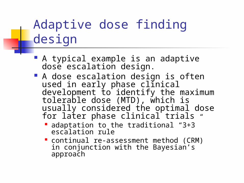
Adaptive dose finding design A typical example is an adaptive dose
escalation design. A dose escalation design is often used
in early phase clinical development to identify the maximum tolerable dose (MTD), which is usually considered the optimal dose for later phase clinical trials adaptation to the traditional “3+3”
escalation rule continual re-assessment method (CRM) in
conjunction with the Bayesian’s approach

Comments How to select the initial dose? How to select the dose range
under study? How to achieve statistical
significance with a desired power with a limit number of subjects?
What are the selection criteria and decision rules?
What is the probability of achieving the optimal dose?

Biomarker-adaptive design A design that allows for adaptation
based on the responses of biomarkers such as genomic markers for assessment of treatment effect.
It involves qualification and standard optimal screening design establishment of predictive model validation of the established
predictive model

Comments A classifier marker usually does not
change over the course of study and can be used to identify patient population who would benefit from the treatment from those do not. DNA marker and other baseline marker for
population selection
A prognostic marker informs the clinical outcomes, independent of treatment.
A predictive marker informs the treatment effect on the clinical endpoint. Predictive marker can be population-specific.
That is, a marker can be predictive for population A but not population B.

Comments Classifier marker is commonly used in
enrichment process of target clinical trials Prognostic vs. predictive markers
Correlation between biomarker and true endpoint make a prognostic marker
Correlation between biomarker and true endpoint does not make a predictive biomarker
There is a gap between identifying genes that associated with clinical outcomes and establishing a predictive model between relevant genes and clinical outcomes

Adaptive treatment-switching design A design that allows the investigator
to switch a patient’s treatment from an initial assignment to an alternative treatment if there is evidence of lack of efficacy or safety of the initial treatment
Commonly employed in cancer trials In practice, a high percentage of
patients may switch due to disease progression

Comments Estimation of survival is a
challenge to biostatistician. A high percentage of subjects
who switched could lead to a change in hypotheses to be tested.
Sample size adjustment for achieving a desired power is critical to the success of the study.
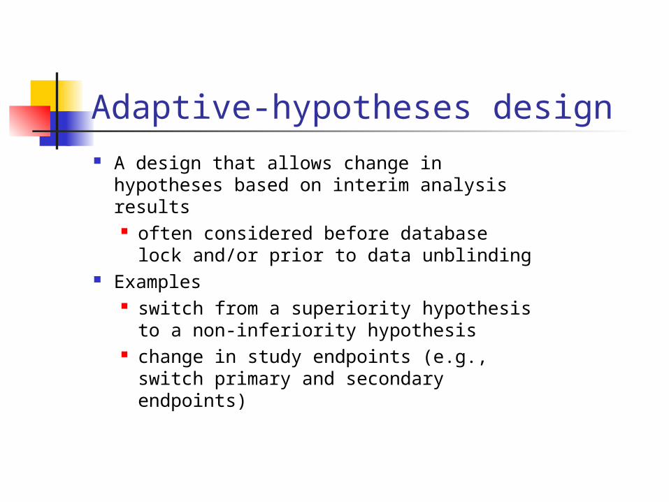
Adaptive-hypotheses design A design that allows change in
hypotheses based on interim analysis results often considered before database
lock and/or prior to data unblinding Examples
switch from a superiority hypothesis to a non-inferiority hypothesis
change in study endpoints (e.g., switch primary and secondary endpoints)

Comments
Switch between non-inferiority and superiority The selection of non-inferiority margin Sample size calculation
Switch between the primary endpoint and the secondary endpoints Perhaps, should consider the switch from
the primary endpoint to a co-primary endpoint or a composite endpoint

Seamless adaptive trial design A seamless adaptive (e.g., phase II/III)
trial design is a trial design that combines two separate trials (e.g., a phase IIb and a phase III trial) into one trial and would use data from patients enrolled before and after the adaptation in the final analysis Learning phase (e.g., phase II) Confirmatory phase (e.g., phase III)

Comments Characteristics
Will be able to address study objectives of individual (e.g., phase IIb and phase III) studies
Will utilize data collected from both phases (e.g., phase IIb and phase III) for final analysis
Questions/Concerns Is it efficient? How to control the overall type I error rate? How to perform power analysis for sample size
calculation/allocation? How to perform a combined analysis if the
study objectives/endpoints are different at different phases?

Multiple adaptive design
A multiple adaptive design is any combinations of the above adaptive designs very flexible very attractive very complicated statistical inference is often difficult,
if not impossible to obtain

Multiple adaptive design
A multiple adaptive design is any combinations of the above adaptive designs very flexible very attractive very complicated statistical inference is often difficult,
if not impossible to obtainvery painful

Possible benefits
Correct wrong assumptions Select the most promising option
early Make use of emerging external
information to the trial React earlier to surprises (positive
and/or negative) May speed up development process

Possible benefits May have a second chance to re-design
the trial after seeing data from the trial itself at interim (or externally)
Sample size may start out with a smaller up-front
commitment of sample size More flexible but more problematic
operationally due to potential bias

Regulatory perspectives May introduce operational bias. May not be able to preserve type I error
rate. P-values may not be correct. Confidence intervals may not be reliable. May result in a totally different trial that is
unable to address the medical questions the original study intended to answer.
Validity and integrity may be in doubt.

Protocol amendments
On average, for a given clinical trial, we may have 2-3 protocol amendments during the conduct of the trial.
It is not uncommon to have 5-10 protocol amendments regardless the size of the trial.
Some protocols may have up to 12 protocol amendments

Protocol amendments
Rationale for changes Clinical Statistical
Review process Internal protocol review IRB Regulatory agencies

Ad hoc adaptations Inclusion/exclusion criteria (slow
enrollment) Changes in dose/dose regimen or
treatment duration (safety concern) Changes in study endpoints (increase
the probability of success) Increase the frequency of data
monitoring or administrative looks Others

Concerns
Protocol amendments may result in a similar but different target patient population
Protocol amendments (with major changes) could result in a totally different trial that is unable to address the questions the original trial intended to answer.
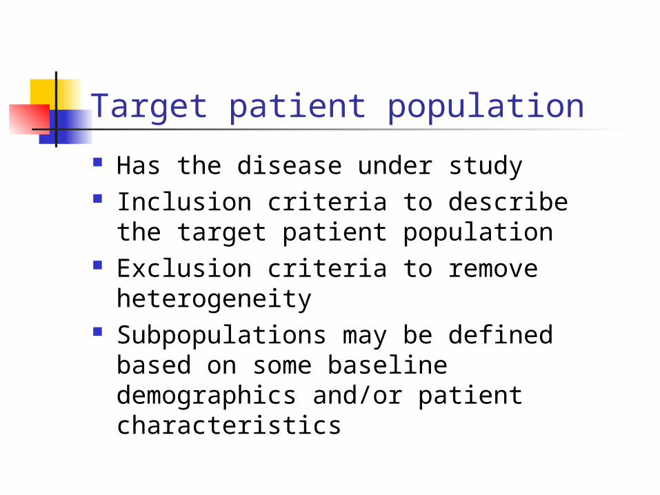
Target patient population
Has the disease under study Inclusion criteria to describe the
target patient population Exclusion criteria to remove
heterogeneity Subpopulations may be defined
based on some baseline demographics and/or patient characteristics

Target patient population Denote target patient population by
, where and are population mean and standard deviation, respectively.
After a modification made to the trial procedures, the target patient population lead to the actual patient population of
( , )
( , )C ( , )Actual Actual

Target patient population
,
1 /
Actual
Actual C
whereC

Target patient population
is usually referred to as the effect
size The effect size after the
modification made is inflated or reduced by the factor of .
“Clinically meaningful difference” may have been changed after the modification (adaptation) is made.

Target patient population
is referred to as a sensitivity index.
When (i.e., there are no impact on the target patient population after the modifications made). In this case, we have =1 (i.e., the sensitivity index is 1).
0 1and C

Sensitivity index
A shift in mean of the target patient population may be offset by the inflation (or reduction) of the variability, e.g., A shift of 10% (-10%) in mean could be
offset by a 10% inflation (reduction) of variability
may not be sensitive due to the masking effect between and C.
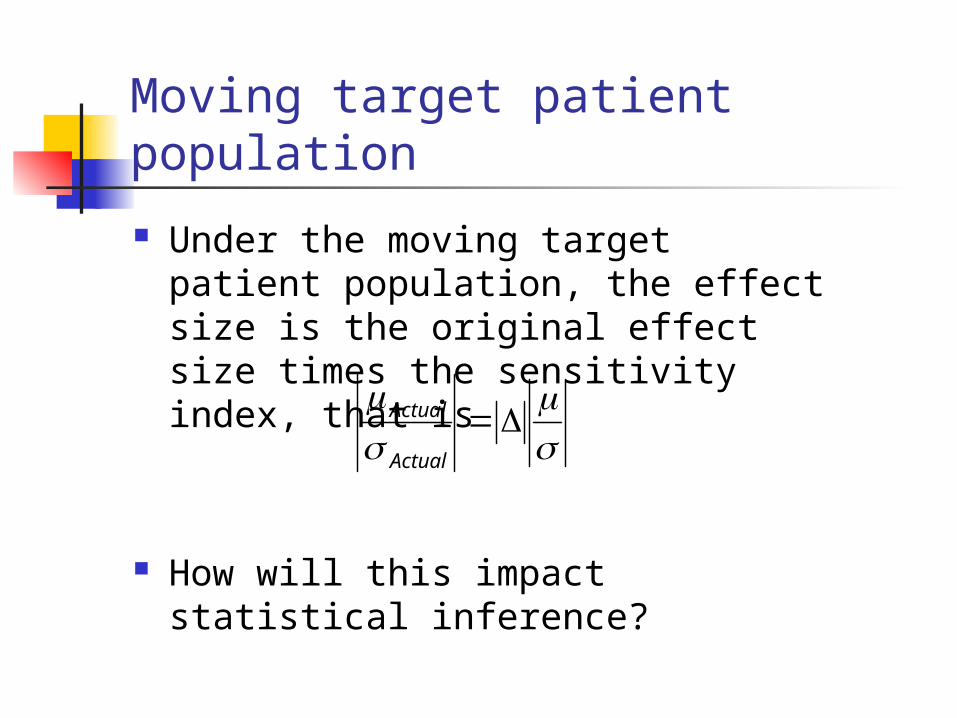
Moving target patient population
Under the moving target patient population, the effect size is the original effect size times the sensitivity index, that is
How will this impact statistical inference?
Actual
Actual

Two possible approaches Adjustment for covariate
Assuming that change in population can be linked by a covariate
Chow SC and Shao J. (2005). J. Biopharm. Stat., 15, 659-666.
Assessment of the sensitivity index Assuming that the shift and/or scale parameter
is random and derive a unconditional inference for the original patient population
Chow SC, Shao J, and Hu OYP (2002). J. Biopharm. Stat., 12, 311-321.
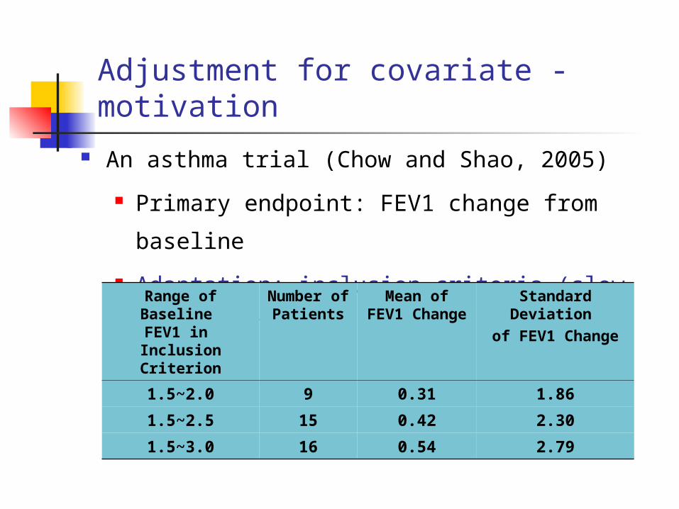
Adjustment for covariate - motivation
An asthma trial (Chow and Shao, 2005)
Primary endpoint: FEV1 change from
baseline
Adaptation: inclusion criteria (slow
enrollment) Range of Baseline FEV1 in Inclusion Criterion
Number of
Patients
Mean of FEV1
Change
Standard Deviation
of FEV1 Change
1.5~2.0 9 0.31 1.86
1.5~2.5 15 0.42 2.30
1.5~3.0 16 0.54 2.79

Adjustment for covariates The idea is to relate the means before
and after protocol amendments by means of some covariates. In other words,
where and are the mean and the corresponding covariate after the protocol amendment, is a given function (linear or non-linear), and is the number of protocol amendments.
,,...,1),( mkxf kk
k kxkth
fm

An example - summary statistics
Range of Baseline FEV1 In Inclusion Criterion
Number of
Patients
Mean ofFEV1
Change
S.D. of FEV1 Change
Mean of Baseline
FEV1
Test drug
1.5~2.0 9 0.31 0.14 1.86
2.0~2.5 15 0.42 0.14 2.30
2.5~3.0 16 0.54 0.16 2.79Placebo 1.5~2.0 8 0.16 0.15 1.82
2.0~2.5 16 0.19 0.13 2.29
2.5~3.0 16 0.20 0.14 2.84

Results of the proposed method
P-value was obtained based on testing for one-sided hypothesis. Classical method ignoring shift in patient population tends to overestimate the
treatment effect.
Estimate for Test Drug
Estimate for Placebo
Difference
Estimated SE
P-value
Covariate-adjusted method
0.33 0.17 0.16 0.057 0.0021
Classical method
0.44 0.19 0.25 0.066 0.0116

Example for sample size calculation
Without
adjustment AdjustmentAdjustme
ntFactor
RHypothesesTotal Each
treatmentTotal Each
treatment
Superiority 200 100 312 156 1.56
Non-inferiority 109 55 170 85 1.56
Equivalence 275 138 431 216 1.56 Note: Two protocol amendment is considered; δ is chosen as
3%.

Endpoint
Goal Model Estimation
Conti.
The WLS method is used to estimate , then
Binary
The ML method is used to estimate , then
: the test treatment : the control treatment
0ii 10 10 ,
0100ˆˆˆ X
0p i
i
e
epi
10
10
1
010
010
ˆˆ
ˆˆ
01
ˆX
X
e
ep
2010 pp
10 ,
)exp(1
)exp(
4321
4321
itit
ititti DD
DDp
11 D
02 D)ˆˆexp(1
)ˆˆexp(ˆ
))ˆˆ(ˆˆexp(1
))ˆˆ(ˆˆexp(ˆ
031
03120
04321
0432110
X
Xp
X
Xp
Summary

Assessment of the sensitivity index
The sensitivity index can be estimated by
where
C
ˆ/ˆ1ˆ
ˆˆˆ Actual
ˆ/ˆˆActualC

Assessment of the sensitivity index There are four scenarios for assessment
of sensitivity index(i) both and are fixed
(ii) is random and is fixed (iii) is fixed and is random (iv) both and are random In addition
The sample size between two protocol amendments is random
The sample size between two protocol amendments is random
Actural ActualActual
ActuralActural Actual
Actural Actual

Sample size adjustment – random location shift
2
22
)(
)(2
zz
Nclassic
2
222/
|)|(
)(2
zz
Nclassic
Hypotheses
Without adjustment Adjustment
Superiority
Non-inferiority
Equivalence
2
222/ )(2
zz
Nclassic
22
2/2
222/
~)(2)1(
~))(1(2
zzm
zzmN
222
22
~)(2)1(
~))(1(2
zzm
zzmN
222/
2
222/
~)(2)1(
~))(1(2
zzm
zzmN
21
210
:
:
aH
H
21
210
:
:
aH
H
||:
||:
21
210
aH
H

2
22
)(
)(2
zz
Nclassic
2
222/
|)|(
)(2
zz
Nclassic
Hypotheses
Withoutadjustment Adjustment
Superiority
Non-inferiority
Equivalence
2
222/ )(2
zz
Nclassic
21
210
:
:
aH
H
21
210
:
:
aH
H
||:
||:
21
210
aH
H
Sample size adjustment – random scale shift
2
0
)(1
2
0
2)(1
222/
)1~(~
)(~~~))(1(2
m
j
tj
m
j
tj
Vv
Vvzzm
N
2
0
)(1
2
0
2)(1
2211
)1~(~
)(~~~))(1(2
m
j
tj
m
j
tj
Vv
Vvzzm
N
2
0
)(1
2
0
2)(1
222/
)1~(~
)(~~~))(1(2
m
j
tj
m
j
tj
Vv
Vvzzm
N

Lecture 2 - Outline
Adaptive dose finding Algorithm-based design Model-based design Design selection
Seamless adaptive design? Relative advantages and limitations Types of two-stage adaptive design Statistical analysis An example
Concluding remarks

Dose finding trials
Fundamental questions Is there any drug effect? What doses exhibit a response
different from control? What is the nature of the dose-
response relationship? What is the optimal dose?

Dose response trial
Response = f(Dose)or
Dose = g(Response)

Dose response trials
ICH E4 (1994) Guideline on Dose-response Information to Support Drug Registration
Randomized parallel dose-response designs Crossover dose-response design Forced titration design
Dose escalation design Optimal titration design
Placebo-controlled titration to endpoint

Dose response relationship
Null hypothesis Alternative
hypotheses
KH ...: 100
KjiaH .........: 0
KKaH 110 ...:
KiaH ......: 0
KaH ....: 10
KiaH ......: 10
KKiaH 10 .......:
KiaH ......: 10
KKiaH 10 ......:


Dose escalation trial Primary objectives
Is there any evidence of the drug effect?
What is the nature of the dose-response?
What is the optimal dose? Principles
Less patients to be exposed to the toxicity
More patients to be treated at potential efficacious dose levels

Dose escalation trial Algorithm-based design
Traditional dose escalation (TER) rule The “3+3” TER The “a+b” TER
Model-based design Continual reassessment method
(CRM) CRM in conjunction with Bayesian
approach

Dose escalation trial Dose limiting toxicity (DLT)
DLT is referred to as unacceptable or unmanageable safety profile which is pre-defined by some criteria such as Grade 3 or greater hematological toxicity according to the US National Cancer Institute’s Common Toxicity Criteria (CTC)
Maximum tolerable dose (MTD) MTD is the highest possible but still
tolerable dose with respect to some pre-specified DLT.

Dose escalation trial The “3+3” TER
The traditional escalation rule is to enter three patients at a new dose level and then enter another three patients when a DLT is observed.
The assessment of the six patients is then performed to determine whether the trial should be stopped at the level or to escalate to the next dose level.
Traditional escalation rule Basically, there are two types of
escalation rules Traditional escalation rule (TER)
Does not allow dose de-escalation Strict traditional escalation rule (STER)
Allow dose de-escalation if two of three patients have DLTs
The “3+3” TER can be generalized to the “a+b” design with and without dose de-escalation.
Continual reassessment method For the method of CRM, the dose-
response relationship is continually reassessed based on accumulative data collected from the trial. The next patient who enters the trial is then assigned to the potential MTD level Dose toxicity modeling Dose level selection Reassessment of model parameters Assignment of next patient

Dose toxicity modeling
Assumptions There is monotonic relationship
between dose and toxicity The biologically inactive dose is lower
than the active dose, which is in turn lower than the toxic dose
Model The logistic model is often considered

Dose toxicity modeling Model
where is the probability of toxicity associated with dose , and and are positive parameters to be determined.
Then, the MTD can be expressed as
where is the probability of DLT at MTD
1)]exp(1[)( axbxp
)1
ln(1
b
aMTD
)(xp
x a b

Dose toxicity modeling Remarks
For an aggressive tumor and a transient and non-life-threatening DLT, could be as high as 0.5
For persistent DLT and less aggressive tumors, could be as low as 0.1 to 0.25
A commonly used value for is somewhere between 0 and 1/3=0.33Crowley (2001)

Dose level selection
General principles It should be low enough to avoid severe
toxicity It should be high enough for observing
some activity or potential efficacy in humans
The commonly used starting dose is the dose at which 10% mortality occurs in mice
)( 10LD

Dose level selection
The subsequent dose levels are usually selected based on the following multiplicative set
where is called the dose escalation factor
11 iii xfx ),...,2,1( ki
if
Dose level selection
Remarks The highest dose level should be
selected such that it covers the biologically active dose, but remains lower than the toxic dose.
In general, CRM does not require pre-determined dose intervals.

Reassessment of model parameters
The key is to estimate the parameter in the response mode An initial assumption or prior
about the parameter is necessary in order to assign patients to the dose level based on the toxicity relationship
The estimate of is continually updated based on cumulative data observed from the trial
a
a

Reassessment of model parameter Remarks – the estimation method
could be a frequentist or Bayesian approach
Frequentist approachMaximum likelihood estimate or least square estimate are commonly considered
Bayesian approach- It requires a prior distribution about the parameter- It provides posterior distribution and predictive probabilities of MTD

Assignment of next patient
The updated dose-toxicity model is usually used to choose the dose level for the next patient. In other words, the next patient enrolled in the trial is assigned to the current estimated MTD based on dose-response model

Assignment of next patient
Remarks Assignment of patient to the most
updated MTD leads to majority of the patients assigned to the dose levels near MTD, which allows a more precise estimate of MTD with a minimum number of patients
In practice, this assignment is subject to safety constraints such as limited dose jump and delayed response

Criteria for design selection
Number of patients expected Number of DLT expected Toxicity rate
Probability of observing DLT prior to MTD Probability of correctly achieving the MTD Probability of overdosing Others
Flexibility of dose de-escalation

An example – radiation theraphy Small size cohort for lower dose levels
Minimize the number of patients at lower dose groups
Majority patients near the MTD Ideally, the last two dose cohorts under study
Flexibility for dose de-escalation Limited dose jump if CRM is used Higher probability of reaching the MTD Lower probability of overdosing Also take moderate AE into consideration

Example - clinical trial simulation Simulation runs = 5,000 Initial dose = 0.5 mCi/kg Dose range is from 0.5 mCi/kg to 4.5 mCi/kg #of dose levels = 6 Modified Fibonacci sequence is considered. That
is, dose levels are 0.5, 1, 1.6, 2.5, 3.5, and 4.7. Maximum dose de-escalation allowed = 1 (for
STER) DLT rate at MTD is assumed to be 1/3=33% Logistic toxicity model is assumed for the CRM Uniform prior is assumed for the CRM #of doses allowed to skip = 0

Summary of Simulation Results (based ob 5,000 simulation runs)
Design
# patients expected (N)
# of DLT expected
Mean MTD (SD)
Prob. of selecting correct MTD
“3+3”TER
15.23 2.8 1.94 (0.507) 0.392
“3+3”STER*
17.59 3.2 1.70 (0.499) 0.208
CRM** 13.82 3.2 2.33 (0.451) 0.696
* Allows dose de-escalation
** Uniform prior was used

What is seamless adaptive design?
A seamless trial design is defined as a design that combines two separate (independent) trials into a single study.
The single study is able to address the study objectives that are normally achieved through the conduct of the two trials.

Seamless adaptive trial design
A seamless adaptive trial design is referred to as a seamless design that applies adaptations during the conduct of the trial.
A seamless adaptive design would use data collected from patients enrolled before and after the adaptation in the final analysis.

Characteristics Combine two separate trials into a
single trial It is also known as a two-stage
adaptive design The single trial consists of two
stages (phases) Learning (exploratory) phase Confirmatory phase
Opportunity for adaptations based on accrued data at the end of learning phase

Advantages Opportunity for saving
Stopping early for safety and/or futility/efficacy
Efficiency Can reduce lead time between the
learning and confirmatory phases Combined analysis
Data collected at the learning phase are combined with those data obtained at the confirmatory phase for final analysis

Limitations (regulatory’s concerns) May introduce operational bias
Adaptations relate to dose, hypothesis and endpoint etc.
May not be able to control the overall type I error rate When study objectives/endpoints are
different at different stages Statistical methods for combined
analysis are not well established Complexity depends upon the
adaptations apply

An example
Two-stage phase II/III study Learning (exploratory) phase
Dose finding Confirmatory phase
Efficacy confirmation
Comparison of type I errors
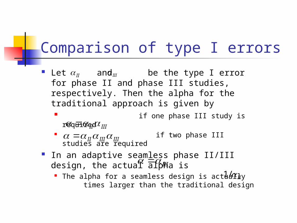
Let and be the type I error for phase II and phase III studies, respectively. Then the alpha for the traditional approach is given by if one phase III study is required if two phase III studies are
required In an adaptive seamless phase II/III
design, the actual alpha is The alpha for a seamless design is actually
times larger than the traditional design
II III
IIIII IIIIIIII
III II/1

Comparison of power Let and be the power for phase
II and phase III studies, respectively. Then the power for the traditional approach is given by if one phase III study is required if two phase III studies are required
In an adaptive seamless phase II/III design, the power is The power for a seamless design is actually
times larger than the traditional design
IIPower IIIPower
IIIII PowerPowerPower *
IIIIIIII PowerPowerPowerPower **
IIIPowerPower IIPower/1
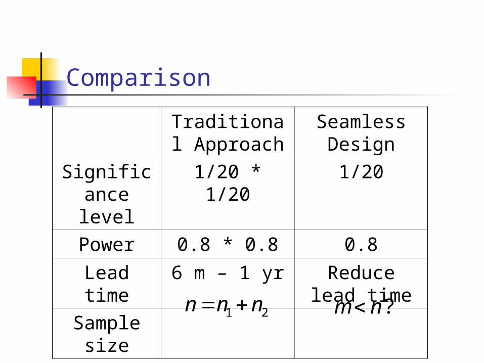
Comparison
Traditional Approach
Seamless Design
Significance level
1/20 * 1/20 1/20
Power 0.8 * 0.8 0.8
Lead time 6 m – 1 yr Reduce lead time
Sample size
1 2n n n ?m n

Seamless adaptive designs
In practice, a seamless adaptive design may combine two separate (independent) trials with similar but different study objectives into a single trial, e.g., A phase II trial for dose selection and a
phase III study for efficacy confirmation In some cases, the study endpoints
considered at the two separate trials may be different, e.g., A biomarker or surrogate endpoint versus
a regular clinical endpoint

Seamless adaptive designs
Category I - SS Same study objectives Same study endpoints
Category II - SD Same study objectives Different study endpoints
Category III - DS Different study objectives Same study endpoints
Category IV - DD Different study objectives Different study endpoints

Categories of two-stage seamless adaptive designs
Study endpoints at different
stages
S D
Study objectives at
different stages
S I=SS II-SD
D III=DS IV=DD

Seamless adaptive designs
Category I - SS Similar to typical group sequential design
Category II - SD Biomarker (or surrogate endpoint or clinical
endpoint with shorter duration) versus clinical endpoint
Category III - DS Dose finding versus early efficacy
Category IV - DD Treatment selection with biomarker (or
surrogate endpoint or clinical endpoint with different treatment duration) versus efficacy confirmation with regular clinical endpoint

Frequently asked questions How to perform power analysis for sample
size calculation/allocation? How to control the overall type I error rate
at a pre-specified level of significance? Especially when the study objectives at
different stages are different How to combine data collected from both
stages for a valid final analysis? Especially when the study objectives
and study endpoints at different stages are different

Statistical analysis for Category I – SS designs
Similar to group sequential trial design with planned interim analyses Can be treated as a multiple-stage trial
design with adaptations Adaptations
Stop the trial early for futility/efficacy Drop the losers Sample size re-estimation
etc

Hypotheses testing
Consider a K-stage design and suppose we are interested in testing the following null hypothesis
where is the null hypothesis at the kth stage
KHHHH 002010 ...:
kH 0

Stopping rules
Let be the test statistic associated with the null hypothesis
Stop for efficacy ifStop for futility ifContinue with adaptations if Where and
kT
,kkT ,kkT
,kkk T
)1,..,1( Kkkk KK

Test based on individual p-values
This method is referred to as method of individual p-values (MIP)
Test statistics
For K=2 (a two-stage design), we have
KkpT kk ,...,1,
)( 1121

Stopping boundaries based on MIP

Test based on sum of p-values
This method is referred to as the method of sum of p-values (MSP)
Test statistic
For K=2 (a two-stage design), we have
KkpTk
iik ,...,1,
1
,)(2
1
),(2
1)(
2121
21
211121
for
for
,
,
21
21

Stopping boundaries based on MSP

Test based on product of p-values
This method is known as the method of products of p-values (MPP)
Test statistic
For K=2 (a two-stage design), we have
KkpT ikik ,...,1,1
),(ln
,ln
211
121
1
121
for
for
,
,
21
21
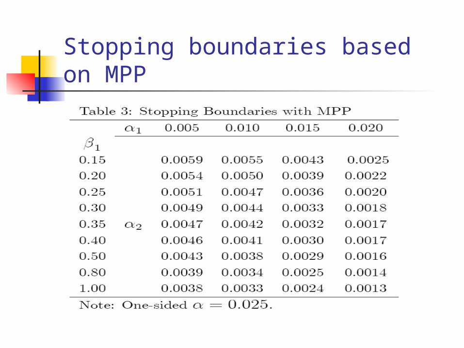
Stopping boundaries based on MPP

Practical Issues Based on MIP, MSP, or MPP, sample size calculation
for achieving the desire power by controlling the overall type I error rate at a pre-specified level of significance can be obtained Statistical methodology was derived under the
assumptions of category I – SS designs Did not address the issue of sample size allocation.
The target patient population may have been shifted after adaptations How do we preserve type I error rate?
Adaptations are made based on “estimates” How this will affect the power?
More adaptations will result in a more complicated adaptive design
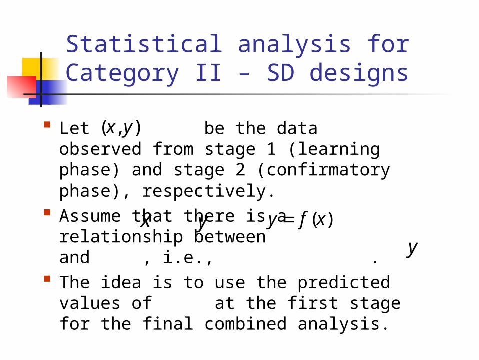
Statistical analysis for Category II – SD designs
Let be the data observed from stage 1 (learning phase) and stage 2 (confirmatory phase), respectively.
Assume that there is a relationship between and , i.e., .
The idea is to use the predicted values of at the first stage for the final combined analysis.
),( yx
x y )(xfy y

Assumptions
and and
and can be related by
where is an error term with zero
mean and variance
)(xE 2)( xVar)(yE 2)( yVar
xy 10
2
x y

Weighted-mean approach
Graybill-Deal estimator
where21 )ˆ1(ˆˆˆ yyGD
22
21
21
//
/ˆ
smsn
sn
.1
1
1
1)ˆ1(ˆ41
//
1)ˆ(
22
21
mnsmsnVar GD

Sample size allocation
Let and be the sample sizes at the first and second stages, respectively.
Also, let . Then the total sample size
where is referred to as the allocation factor.
nm
(1 )N n fn
n m
1/ f

Sample size allocation
For testing the hypothesis of equality, we have
where
and
0
10
)1(
)1(811
)(2 Nrr
Nn
222/
20 /)( zzN
2221 /r

Remarks
Following similar idea, formulas for sample size calculation/allocation for testing the hypothesis of superiority, non-inferiority, and equivalence can also be derived.
Similar idea can be applied to count data (binary responses) and time-to-event data assuming that there is a well-established relationship between the two study endpoints at different stages.

Category II – SD designsCategory II – SD designs (continuous and binary endpoints)(continuous and binary endpoints)
Hypotheses Testing
Continuous Endpoint Binary Response
Equality
Non-inferiority(δ < 0)
Superiority(δ > 0)
Equivalence
11
1(1 1 8(1 ) )
2n AB A C
11
1(1 1 8(1 ) )
2n BD D C
11
1(1 1 8(1 ) )
2n DB D C
11
1(1 1 8(1 ) )
2n EB E C
2 222 1 1 2 2
1 22 1
( ) ( ( ) ( ))
( )
z zn
2 221 1 2 2
1 22 1
( ) ( ( ) ( ))
( )
z zn
2 221 1 2 2
1 22 1
( ) ( ( ) ( ))
( )
z zn
2 221 1 2 2
1 22 1
( ) ( ( ) ( ))
( | |)
z zn

Category II – SD designsCategory II – SD designs (time-to-event data)(time-to-event data)
Hypotheses Testing
Weibull Distribution Cox’s Proportional Hazard Model
Equality
Non-inferiority(δ < 0)
Superiority(δ > 0)
Equivalence
2 12
1 2
( ) ( )
( )T R
T R
z zn
M M
2 1
21 2
( ) ( )
( )T R
T R
z zn
M M
2 1
21 2
( ) ( )
( )T R
T R
z zn
M M
2 1
21 2
( ) ( )
(| | )T R
T R
z zn
M M
1 1 1 1
22
1 2 21 2
( )
( )T R T R
z zn
b p p u p p u
2
1 2
( ) ( <0)
( )
z zn
e b K
2
1 2
( ) ( 0)
( )
z zn
e b K
22 2
1 2
( )
( | |)
z zn
e b K
Note
The definitions of the notations given in the previous slides can be found in following reference
ReferenceChow, S.C. and Tu, Y.H. (2008). On two-stage seamless adaptive design in clinical trials. Journal of Formosan Medical Association, 107, No. 12, S51-S59.

Remarks
One of the key assumptions in the proposed method is that there is a well-established relationship between the endpoints Biomarker vs clinical endpoint Same clinical endpoint with different
durations When there is a shift in patient population,
the proposed method needs to be modified Protocol amendments

An example – the HCV study
Study objectives – to evaluate the safety and efficacy of a test treatment for treating patients with hepatitis C virus (HCV) genotype 1 infection Dose selection (phase II) Efficacy confirmation (phase III)
Study design A two-stage phase II/III seamless adaptive
design Subjects are randomly assigned to five
treatments (4 active and one placebo)
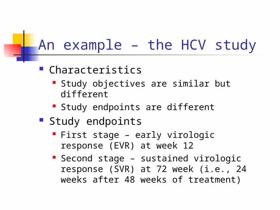
An example – the HCV study
Characteristics Study objectives are similar but different Study endpoints are different
Study endpoints First stage – early virologic response
(EVR) at week 12 Second stage – sustained virologic
response (SVR) at 72 week (i.e., 24 weeks after 48 weeks of treatment)

Adaptations considered Two planned interim analyses
The first interim analysis will be performed when all Stage 1 subjects have completed study Week 12.
The second interim analysis will be conducted when all Stage 2 subjects have completed Week 12 of the study and about 75% of Stage 1 subjects have completed Stage 1 treatment.
The O’Brien-Fleming type of boundaries are applied.

Criteria for dose selection at Stage 1
Dose selection is performed based on the precision analysis. Based on EVR, the dose with
highest confidence level for achieving statistical difference (i.e., the observed difference is not by chance alone) as compared to the control arm is selected.

An example – the HCV study
Notations : treatment effect of the ith dose group at
the jth stage based on surrogate endpoint : treatment effect of the ith dose group at
the
jth stage based on regular clinical endpoint
i=1,…, k (dose group)
j=1,2 (stage)
jiE ,
ji ,

Study design of the HCV study
Two-stage seamless adaptive design
Stage 1 Stage 2
Multiple stage design
1st interim analysis
Decision-making
End of Stage 1
2nd interim analysis
Sample size re-estimation
End of study
Stage 1 Stage 2 Stage 3 Stage 4

An example – the HCV study
This two-stage seamless design can then be viewed as a 4-stage design
Hypotheses of interest
kiH
kiH
i
i
,,1,0:
,,1,0:
2,2,0
1,1,0

An example – the HCV study Testing procedure
Stage 1 If , then stop the trial. If , then treatment will proceed
to Stage 2, where Stage 2
If , then
stop the trial. If but then move to Stage
3.
11,ˆmax ci
2,21*, ci 1,21,2 cT
1,22*,21
21*,
21
11,2
ˆˆ cnn
n
nn
nT ii
1,1
ˆmaxarg* iki
i
*iE11,
ˆmax ci

An example – the HCV study Stage 3
If
,
stop the trial; otherwise move to Stage 4. Stage 4
If
,
reject .
32*,21
21*,
21
12,3 ˆˆ c
nn
n
nn
nT ii
2,0H
42*,321
22,3
321
12,4 ˆ c
nnn
nT
nnn
nT i
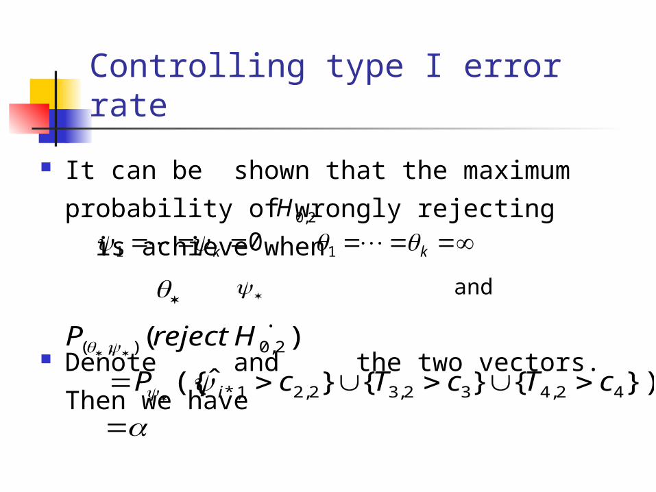
Controlling type I error rate
It can be shown that the maximum
probability of wrongly rejecting is
achieve when
and .
Denote and the two vectors. Then we
have
2,0H
k 1
}){}{}ˆ({
)(
42,432,32,21*,
2,0),(
cTcTcP
HrejectP
i
01 k

Sample size calculation
Power can be evaluated at and
Denote and the two vectors. Then we have
2111 , kk
*2111 , kk
*
1
),ˆ,*}{}{}ˆ({
),ˆ,*(
)(
1,21,211*,42,432,32,21*,*)*,(
1,21,211*,*
2,0*)*,(
cTckicTcTcP
cTckiP
HrejectP
ii
i

Sample size calculation
Let N be the total number. Then
Similar to Thall, Simon and Ellenburg (1988), we can choose the parameters such that
is minimized.
),ˆ,,ˆ(2
)ˆ(2)1()(
32,32,21*,1,21,211*,3
11*,21
cTccTcPn
cPnnkNE
ii
i
*)*,(2
1),(
2
1** NENE

Remaining issues
How about sample size allocation? Is the usual O’Brien-Fleming type of
boundaries appropriate? How to combine data collected
from both stages for a valid final analysis?
What if there is a shift in target patient population?
Can clinical trial simulation help?

Remarks
The usual sample size calculation for a two-stage design with different study objectives/endpoints needs adjustment.
One of the key assumptions is that there is a well-established relationship between different endpoints. This relationship may not exist or cannot be
verified in practice. When there is a shift in patient population
(e.g., as the result of protocol amendments), the above method needs to be modified.

Future perspectives Well-understood design
Group sequential design Less well-understood design
Adaptive group sequential design Adaptive dose finding Two-stage seamless adaptive design
For less well-understood designs, they should be used with caution
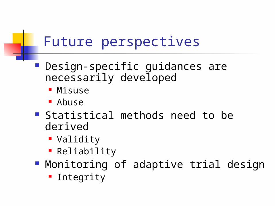
Future perspectives
Design-specific guidances are necessarily developed Misuse Abuse
Statistical methods need to be derived Validity Reliability
Monitoring of adaptive trial design Integrity

Concluding remarks Clinical
Adaptive design reflects real clinical practice in clinical development.
Adaptive design is very attractive due to its flexibility and efficiency.
Potential use in early clinical development. Statistical
The use of adaptive methods in clinical development will make current good statistics practice even more complicated.
The validity of adaptive methods is not well established.
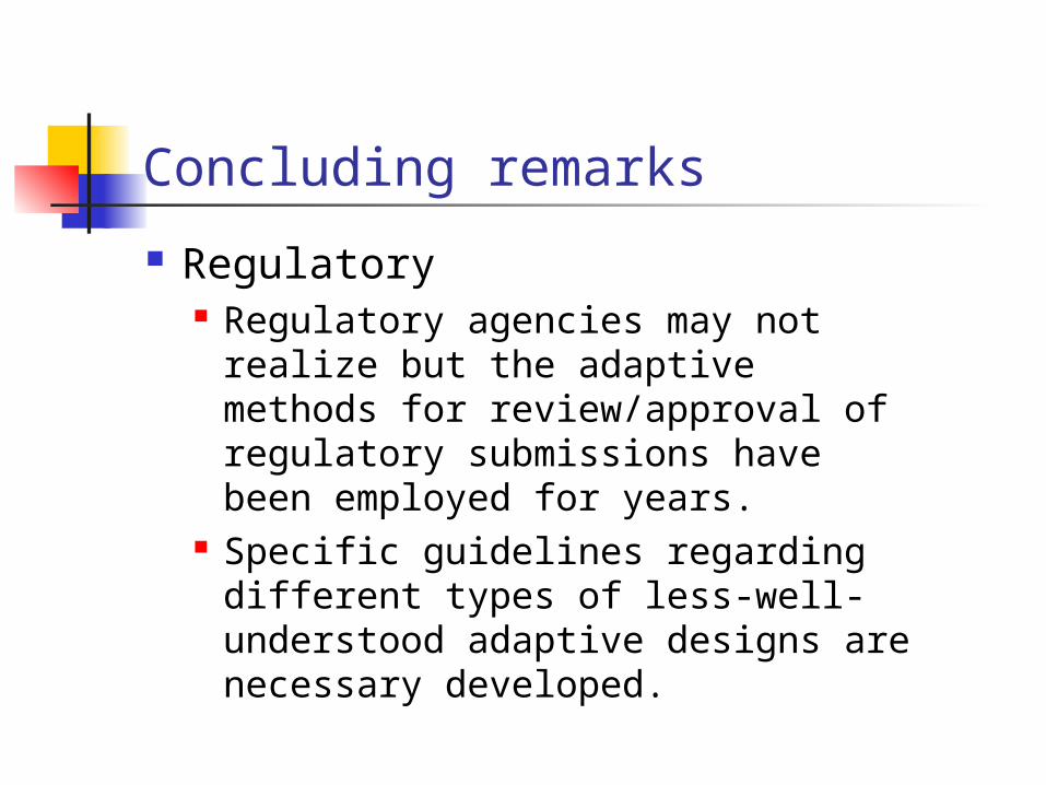
Concluding remarks
Regulatory Regulatory agencies may not realize but
the adaptive methods for review/approval of regulatory submissions have been employed for years.
Specific guidelines regarding different types of less-well-understood adaptive designs are necessary developed.
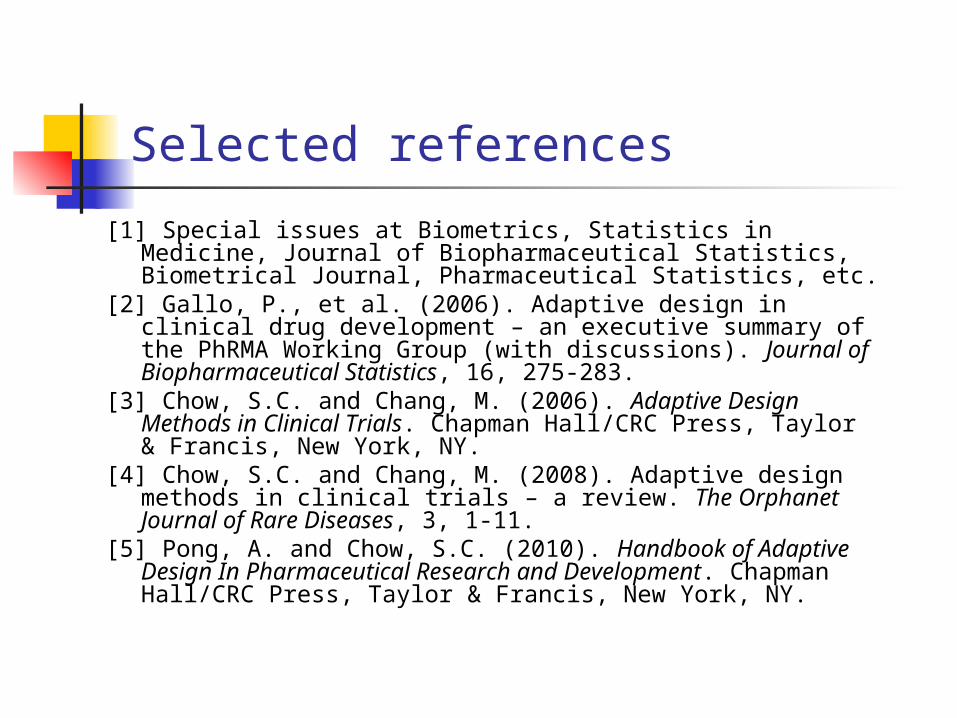
Selected references
[1] Special issues at Biometrics, Statistics in Medicine, Journal of Biopharmaceutical Statistics, Biometrical Journal, Pharmaceutical Statistics, etc.
[2] Gallo, P., et al. (2006). Adaptive design in clinical drug development – an executive summary of the PhRMA Working Group (with discussions). Journal of Biopharmaceutical Statistics, 16, 275-283.
[3] Chow, S.C. and Chang, M. (2006). Adaptive Design Methods in Clinical Trials. Chapman Hall/CRC Press, Taylor & Francis, New York, NY.
[4] Chow, S.C. and Chang, M. (2008). Adaptive design methods in clinical trials – a review. The Orphanet Journal of Rare Diseases, 3, 1-11.
[5] Pong, A. and Chow, S.C. (2010). Handbook of Adaptive Design In Pharmaceutical Research and Development. Chapman Hall/CRC Press, Taylor & Francis, New York, NY.


![I^H` 0HTZ 4H[[LS 3H`Z HUK*OL]YVSL[mediumcontrol.com/clients/elizabethshein/resume.pdf · elizabeth-shein-resume-20150312 Author: Elizabeth Shein Created Date: 3/12/2015 12:17:09 PM](https://static.fdocuments.in/doc/165x107/5fdf8b157c46794880730ab1/ih-0htz-4hls-3hz-hukolyvsl-elizabeth-shein-resume-20150312-author-elizabeth.jpg)