Adaptive Correctness Monitoring for Wireless Sensor Networks Using Hierarchical ...€¦ · ·...

8

Adaptive Correctness Monitoring for WirelessSensor Networks Using HierarchicalDistributed Run-Time Invariant Checking

DOUGLAS HERBERT, VINAITHEERTHAN SUNDARAM, YUNG-HSIANG LU,SAURABH BAGCHI, and ZHIYUAN LI

Purdue University

This article presents a hierarchical approach for detecting faults in wireless sensor networks(WSNs) after they have been deployed. The developers of WSNs can specify “invariants” thatmust be satisfied by the WSNs. We present a framework, Hierarchical SEnsor Network Debugging(H-SEND), for lightweight checking of invariants. H-SEND is able to detect a large class of faultsin data-gathering WSNs, and leverages the existing message flow in the network by buffering andpiggybacking messages. H-SEND checks as closely to the source of a fault as possible, pinpointingthe fault quickly and efficiently in terms of additional network traffic. Therefore, H-SEND is suitedto bandwidth or communication energy constrained networks. A specification expression is pro-vided for specifying invariants so that a protocol developer can write behavioral level invariants.We hypothesize that data from sensor nodes does not change dramatically, but rather changesgradually over time. We extend our framework for the invariants that includes values determinedat run-time in order to detect data trends. The value range can be based on information local to asingle node or the surrounding nodes’ values. Using our system, developers can write invariantsto detect data trends without prior knowledge of correct values. Automatic value detection can beused to detect anomalies that cannot be detected in existing WSNs. To demonstrate the benefits ofrun-time range detection and fault checking, we construct a prototype WSN using CO2 and tem-perature sensors coupled to Mica2 motes. We show that our method can detect sudden changes ofthe environments with little overhead in communication, computation, and storage.

This article is based on the paper “Detection and Repair of Software Errors in Hierarchical SensorNetworks” by Douglas Herbert, Yung-Hsiang Lu, Saurabh Bagchi, and Zhiyuan Li, which appearsin the Proceedings of the IEEE International Conference on Sensor Networks, Ubiquitous, andTrustworthy Computing, 403–410. c© 2006 IEEE.Doug Herbert was supported by the Tellabs Fellowship from Purdue’s Center for Wireless Systemsand Applications. This project is supported in part by the National Science Foundation grant CNS0509394 and by Purdue Research Foundation. Any opinions, findings, and conclusions or recom-mendations in the projects are those of the authors and do not necessarily reflect the views of thesponsors.Authors’ address: School of Electrical and Computer Engineering, Department of ComputerScience, Purdue University, West Lafayette, IN 47907; email: {herbertd, vsundar, yunglu, andsbagchi}@purdue.edu; [email protected] to make digital or hard copies of part or all of this work for personal or classroom use isgranted without fee provided that copies are not made or distributed for profit or direct commercialadvantage and that copies show this notice on the first page or initial screen of a display alongwith the full citation. Copyrights for components of this work owned by others than ACM must behonored. Abstracting with credit is permitted. To copy otherwise, to republish, to post on servers,to redistribute to lists, or to use any component of this work in other works requires prior specificpermission and/or a fee. Permissions may be requested from Publications Dept., ACM, Inc., 2 PennPlaza, Suite 701, New York, NY 10121-0701 USA, fax +1 (212) 869-0481, or [email protected]© 2007 ACM 1556-4665/2007/09-ART8 $5.00 DOI 10.1145/1278460.1278462 http://doi.acm.org/10.1145/1278460.1278462

ACM Transactions on Autonomous and Adaptive Systems, Vol. 2, No. 3, Article 8, Publication date: September 2007.

8:2 • D. Herbert et al.

Categories and Subject Descriptors: C.2.1 [Computer-Communication Networks]: Network Ar-chitecture and Design—Distributed networks, network communications, packet-switching networks

General Terms: Reliability, Verification, Design

Additional Key Words and Phrases: Invariants, correctness monitoring, run-time, tools, fault tol-erance and diagnostics, in-network processing and aggregation, network protocols, programmingmodels and languages, data integrity

ACM Reference Format:Herbert, D., Sundaram, V., Lu, Y.-H., Bagchi, S., and Li, Z. 2007. Adaptive correctness monitoring forwireless sensor networks using hierarchical distributed run-time invariant checking. ACM Trans.Autonom. Adapt. Syst. 2, 3, Article 8 (September 2007), 23 pages. DOI = 10.1145/1278460.1278462http://doi.acm.org/10.1145/1278460.1278462

1. INTRODUCTION

Wireless Sensor Networks (WSNs) enable continuous data collection or rareevent detection in large, hazardous or remote areas. The data being collectedcan be critical. Detecting indoor air quality or tracking tank movement are twoexamples from civilian and military domains. WSNs are comprised of manysensors that may fail for many reasons. Faults may come from incorrect sensornetwork protocols. Distributed protocols are widely recognized as being diffi-cult to design [Tel 1991]. WSNs present unique challenges because of the lackof sophisticated debugging tools and the difficulty of testing after deployment.Even after extensive testing, faults may still occur due to environment condi-tions, such as high temperatures. While this is true of many systems, this isespecially true with WSNs as they are in situ in physical environments thatmay be changing over the period of deployment. Regardless of design or valida-tion, sensors can still be damaged by unexpected factors such as storms, hail,animals, or flood.

Run-time techniques can detect faults in order to maintain high-fidelity datain the presence of possible faults from design, implementation, or a hostile en-vironment. Earlier work for run-time observation in wired networks [Diaz et al.1994; Khanna et al. 2004; Zulkernine and Seviora 2002] does not directly ap-ply to WSNs as they are resource-limited. It is essential to minimize the over-head of storage, computation, and communication in observation and detection.We developed a framework called Hierarchical SEnsor Network Debugging(H-SEND) [Herbert et al. 2006] to observe node conditions and network trafficfor detecting symptoms of faults. H-SEND differs from existing work in thatit is specialized for large scale WSNs. H-SEND has four key steps: (a) Duringprogram development, a programmer can specify important properties as “in-variants” that should never be violated in the network’s operation. (b) Whenthe program is compiled, the code for checking invariants is automatically in-serted. An invariant may be checked locally by an individual node or remotelyby sending messages to another node for detecting faults that cannot be deter-mined by a single sensor node. (c) After deployment, the inserted code is usedto detect abnormal behavior of the network. An anomaly is detected when aninvariant is violated. An invariant may include a fixed value determined at com-pile time, or a data trend observed at run time. Once detected, an anomaly can


Adaptive Correctness Monitoring for Wireless Sensor Networks • 8:3

trigger several actions, such as increasing logging details or reporting faults tothe base station. (d) After a fault is detected, it is reported to the programmerand a new program is uploaded to the relevant nodes through multi-hop wire-less reprogramming. H-SEND is designed for WSNs with the following specialconsideration:

(a) Our approach has small overhead in storage, computation, and communi-cation. H-SEND checks invariants through a hierarchy without sending allobserved variables to a central location for detection. Instead, invariants arechecked at the closest nodes where the requisite information is available.We present the analysis of the overhead in Section 4.4.

(b) H-SEND assists programmers by automatically (or semi-automatically) de-termining where to insert invariant checking code and when to send mes-sages that include observed variables. A programmer only needs to specifythe invariants and the variables to be observed. Our tool can determinethe locations to insert code for checking invariants and to send observedinformation.

(c) Using H-SEND, faults may be detected by comparing the values from mul-tiple nodes. H-SEND can observe data trends that are determined onlyat run-time, such as temperature changes in a wildlife preserve. In nor-mal operations, temperatures do not change suddenly. A sudden rise oftemperature may be caused by fire and must be reported immediately. Wecan compare current values against historical values on an individual node(temporal trend) or the current values on surrounding nodes (spatial trend).

(d) H-SEND can handle WSNs with heterogeneous nodes that are organizedas hierarchies. Different nodes may check different types of invariants andalso perform remote checking when observed information is aggregated.

We construct a prototype WSN to demonstrate H-SEND through a leaderelection and data gathering protocol in a hierarchical configuration. Some in-variants are local to a node but others are collective to a cluster or the entirenetwork. We choose a representative leader election protocol called LEACH(Low-Energy Adaptive Clustering Hierarchy) Heinzelman et al. [2000, 2002].LEACH assigns cluster heads in a near round-robin manner to evenly distributeenergy drain. A set of invariants is inserted into the application code. We de-tect both temporal and spatial trends based on data collected from our CO2 andtemperature sensors coupled to Mica2 motes with custom built power supplyand interface circuits. Figure 1 shows the measurement of CO2 in a campuslounge where some students find an ideal place to nap. Learning would sufferif the level of CO2 in a classroom was this high. This indicates the necessity ofmonitoring CO2 level in indoor environments. Our method can detect suddenCO2 level increases, such as at the start of a class, triggering an invariant viola-tion which can increase air flow to the room. We use simulations to measure theoverhead of invariant augmented code in our approach. The experiments andsimulations show that data trends can be observed and used to detect anomalieswith small overhead.



Fig. 1. CO2 levels observed in multiple locations in student lounge.

Fig. 2. Overview of the framework for fault detection, propagation, diagnosis, and repair.

2. RELATED WORK

2.1 Sensor Programming Environment and Simulation

A typical hierarchical sensor network is shown in Figure 2. Once sensor networksoftware is created by a developer, it may be uploaded to individual sensors byutilizing distributed propagation techniques over a radio link [Hui and Culler2004] as illustrated in Figure 2. Berkeley Mica Motes [Hill and Culler 2002]are widely used sensor nodes for experiments. Mica nodes use TinyOS as therun-time environment. TinyOS provides an event-based simulator, TOSSIM,which can be used to simulate a network of varying node sizes [Levis et al.2003]. TOSSIM compiles from the same source code as the Mica platform. Ourexperiments use TOSSIM because it easily scales to large numbers of nodes.TOSSIM provides deterministic results so it is a better test bed in contrast tothe nondeterministic results provided by real-life execution. Finally, TOSSIMallows us to separate instrumentation code from the actual code running on eachnode so we can measure the nodes’ behavior without perturbing the network’snormal operations. To increase the accuracy of our simulation, we inject sensedvalues from actual sensors, and use these values to simulate data collection.



2.2 Program Monitoring and Profiling

Program monitoring and profiling have been developed for wired networks[Diaz et al. 1994; Khanna et al. 2004; Zulkernine and Seviora 2002]. One ap-proach is to directly modify binary code [Kumar et al. 2005] using binary anal-ysis tools to insert instrumentation code to monitor program operation. Thisapproach detects faults in programs while operating in a real environment.DIDUCE [Hangal and Lam 2002] instruments source code and formulates hy-potheses of possible rules about correct program operations. DIDUCE uses ma-chine learning by starting with strict rules that are gradually relaxed to allownew program behavior. Formal methods have been used to prove program’s be-havior from a theoretical view [Hamlet 2005]. Analysis of program operationswith an SQL-like language is used for correctness monitoring in [Goldsmithet al. 2005]. Adding hardware to monitor memory changes for checking at run-time is discussed in [Zhou et al. 2005; Wang et al. 2006]. Several studies discusshow to find invariants for programs [Perkins and Ernst 2004; Ernst et al. 2001;Yen et al. 2001]. These studies provide the foundation for using invariants inWSNs, but existing approaches cannot be directly applied to WSNs because theobservation algorithms may execute at a location far away from nodes wheredata are collected, adding significant network traffic to propagate data. SinceWSNs are resource-limited, invariant checking must be efficient in using thesensor nodes’ communication and computation.

2.3 Clustering

WSNs are distributed systems. Distributed algorithms have been studied in[Lynch 1996]. WSNs differ from wired distributed systems because sensorshave stringent resource constraints, including energy, storage, and computationcapability. To conserve energy, some routing protocols use hierarchies amongsensor nodes [Soro and Heinzelman 2005; Younis et al. 2002], preventing allnodes from relaying all messages (routing by “flooding”). Sensor nodes are oftendivided into clusters and a special node or “cluster head” (CH) in each clusterrelays messages between clusters or to a base station. Cluster heads can bechosen in several ways. If sensor nodes are heterogeneous, the nodes that havemore resources are selected as cluster heads. For homogeneous nodes, they cantake turns playing the role of the cluster head through leader election protocols[Dolev et al. 1997; Nakano and Olariu 2002; Singh 1996].

2.4 Fault Detection and Recovery

Studies have been conducted to observe run-time behavior for wired networks[Diaz et al. 1994; Khanna et al. 2004; Zulkernine and Seviora 2002]. In thesestudies, the observed node and the observer are different so this approach pro-vides several advantages: (a) An observer may be a monolithic entity with per-fect knowledge of the observed node. (b) An observer may be fault-proof ormay only fail in constrained ways, such as fail-silence. (c) An observer mayhave abundant resources. Fault observation in resource-constrained WSNs hasalso been studied. Several projects use local observation whereby nodes over-see traffic passing through the neighbor nodes [Nasipuri et al. 2001; Pirzada



and McDonald 2004; Marti et al. 2000; Buchegger and Boudec 2002; an Huangand Lee 2003; Khalil et al. 2005, 2006]. Each node can both sense the environ-ment and observe other nodes. Previous work uses local observation to buildtrust relationships among nodes in networks [Buchegger and Boudec 2002;Pirzada and McDonald 2004], detect attacks [Marti et al. 2000; an Huang andLee 2003], or discover routes with certain properties, such as a node becomingdisconnected [Nasipuri et al. 2001]. an Huang et al. [2003] propose distributedintrusion observation for ad hoc networks. Their paper uses machine learningto choose the parameters needed to accurately detect faults. Intrusion detectionsystems exist [Vigna et al. 2004; Medidi et al. 2003]. However, the knowledgein these systems is built by each individual node without the need for coordi-nation, and no information is transmitted to remote nodes. Smith et al. [1997]detect protocol faults for ad hoc networks. After faults are detected, new pro-grams may be sent to the sensor nodes through the same wireless network fortransmitting data. Deluge [Hui and Culler 2004] allows program replacementby propagating new program images over wireless networks. In our previouswork [Khalil et al. 2005], we presented a method to enable neighbor observa-tion in resource-constrained environments and to provide the structures andthe state to be maintained at each node. We analyze the capabilities and thelimitations of local observation for WSNs.

2.5 Estimation and Approximate Agreement

A summary of approximate agreement upon a single value is provided by Lynch[1996]. Lamport et al. [1982] formulate the Byzantine Generals problem of gain-ing distributed consensus in the presence of faults. It is shown that for 3N + 1nodes reporting binary (true or false) data, the correct value can be determinedif no more than N nodes report incorrect values. Maheney et al. [1985] showthat continuous value estimation requires fewer correct nodes to achieve con-sensus for a given degree of fault tolerance. Two-thirds of nodes performingcorrectly guarantee convergence of their algorithm. If between one-third andtwo-thirds of nodes perform correctly, their algorithm can detect that too manyfaults have occurred to determine correctness or show that the divergence isbounded. Marzullo [1990] provides an algorithm to obtain inexact agreementfor continuously valued data, and presents a method of transforming a pro-cess control program for better fault tolerance. Marzullo demonstrates how tomodify specifications to accommodate uncertainty.

2.6 Benefits of CO2 Monitoring

Many studies have provided the relationship between the concentration of car-bon dioxide (CO2) and indoor air quality [Seppanen et al. 1999; Erdmann et al.2002; Milton et al. 2000]. In an office building, occupants (people) are the pri-mary source of CO2. High levels of CO2 (usually above 1000 parts per million,or ppm) are connected with sick building syndrome (SBS) symptoms. As a ref-erence, the CO2 level in outdoor air is usually below 350 ppm. Even thoughCO2 levels are not a direct indicator of indoor air quality, the CO2 levels canprovide indirect information of ventilation efficiency, SBS, respiratory disease,



Fig. 3. Device for measuring airflow volume.

and occupant absence. Every year, approximately 4 million deaths occur due toviral respiratory infections [Liao et al. 2005]. Liao et al. [2005] develop a modelfor the infection of influenza and severe acute respiratory syndrome (SARS) forindoor environment. Studies show that increasing ventilation can reduce theinfection of airborne diseases [Yu et al. 2004; Liao et al. 2005; Myatt et al. 2004;Rudnick and Milton 2003]. Ventilation volume for uninstrumented spaces iscommonly collected with a device that fits over the supply vent, and forces airto flow through the measurement device, as shown in Figure 3. This methodmeasures only one data point. We use multiple CO2 sensors as indicators ofventilation volume, and transmit sensor readings to a central location usingwireless sensor nodes. Sensor data are collected continuously and automati-cally without the need of a human worker. We believe this type of applicationwill be widely deployed because of (a) the low cost of sensors, and (b) the realtime feedback they provide in control systems. It has been shown that demandcontrolled ventilation can save energy [Haghighat and Donnini 1992; Emmerich1996]. WSNs substantially reduce the cost by removing the need for long cablesfor communication between sensors and the control center.

2.7 Comparison and Our Contributions

Table I summarizes the capabilities of several related projects. In this table, weadopt the following definitions:

—“Mobility” is the ability of nodes to move over time;—“Hierarchy” refers to a tiered arrangement of nodes;—“Learning” indicates the ability to estimate correct values at run time;—“Resource Efficient” shows if hardware resource usage is a concern;—“Aggregation” is the ability to combine data;—“Designed for Security” states whether security is a main goal of the design;—“Add/Remove nodes” shows if it is possible to change the number of nodes at

run-time.



Table I. Matrix of Capabilities of Fault Observation Methods: Sympathy [Ramanathan et al.2005], DICAS [Khalil et al. 2005], Daicon [Ernst et al. 2001], DIDUCE [Hangal and Lam 2002]

H-SEND Sympathy DICAS Send to Base Daicon DIDUCEMobility Yes Yes Yes Yes No NoHierarchy Yes No Yes Yes No NoLearning Yes Not Yet No No Yes YesResourceEfficient Yes Yes Yes No No NoAggregation Yes Yes No Yes No NoDesignedfor Security No No Yes No No NoAdd/RemoveNodes Yes No Yes Yes No No

Sympathy [Ramanathan et al. 2005] transmits metrics such as network linkquality and routing stability back to the base station for analysis. Sympathyassumes high throughput of the network and all data for correctness checkingare sent to the base station. Dicas [Khalil et al. 2005] places additional nodes tomonitor wireless communication for detecting faults. Send-to-base is a simplemethod where the developer manually inserts code to send all variables to bemonitored back to the base station. Daicon [Ernst et al. 2001] and DIDUCE[Hangal and Lam 2002] observe the behavior of programs to automatically cre-ate invariants; developers are not required to specify invariants. Automatic cre-ation is performed by first creating strict invariants. As the programs execute,the invariants are gradually relaxed to accommodate new correct behavior. Nei-ther Daicon nor DIDUCE is designed for distributed or resource-constrainedsystems like WSNs.

This article extends our previous work [Herbert et al. 2006] where weintroduce-observing variables specified by a developer through invariants todetect faults. This prior work used invariants determined at compile-time. Inaddition, we have investigated capturing data trends over time in [Herbertet al. 2007a], where we used data modeling to reduce the amount of transmis-sion overhead. We explored the benefits CO2 and temperature monitoring inreal world applications in [Herbert et al. 2007b]. This article includes a detailedstudy of how to use the same infrastructure with the addition of invariants thathave run-time determined parameters, and validates this approach on datacollected from real sensors. We deploy a WSN to measure indoor CO2 and tem-perature levels, and demonstrate that our framework can correctly detect datatrends and sudden changes of the levels as violations of invariants.

3. TECHNIQUES FOR FAULT DETECTION, DIAGNOSIS, AND REPAIR

3.1 Overview

Our system determines the health of a WSN by detecting software faults orsudden changes of data trends, propagating the information to the base station,assisting a programmer to diagnose the faults, and then distributing correctsoftware after the programmer fixes the faults. Our approach addresses “Whatis observed and when?” and “How is a fault detected?”



3.1.1 What Is Observed and When?. Invariants are classified in severalways:

Local invariants are formed from variables resident on the same node (hence-forth referred to as local variables, not to be confused with local variables withina function) only and multinode invariants from a mix of local and nonlocalvariables. Local invariants can be checked at any point where the constituentvariables are in scope, while remote invariants can be checked when the set ofnetwork messages carrying all the nonlocal variables have been successfullyreceived and the local variables are in scope.

Stateless invariants and stateful invariants. Stateless invariants are alwaystrue for the node, irrespective of the node’s operation states. Stateful invariantsare true only when the node is in a particular execution state.

Compile-time determined invariants and Run-time determined invariants.Compile-time determined invariants compare variables and program condi-tions against values that do not change. Run-time determined invariants usespatial trending to compare variables and program conditions against otherneighboring nodes. Temporal trending compares against prior history. An exam-ple of a compile-time determined invariants is “Sensed temperature is between10 and 30 degrees Celsius.” An example of a run-time determined invariantutilizing history is “Temperature does not change by more than 10% in a periodof 60 seconds.” A run-time determined invariant can check the condition “Allnodes report temperatures that are within 1 standard deviation of each other.”H-SEND allows different classes of invariants to detect different faults.

3.1.2 How Is a Fault Detected?. A fault is detected when one or multi-ple invariants are violated. The verification of a local invariant involves somecomputation without additional communication. One of the benefits of perform-ing temporal trending is that expensive communication is required only whena fault is detected. The verification of a remote invariant involves additionalcommunication. Spatial trending requires communication energy to propagatevalues, but requires less memory because a history buffer does not need to bekept. WSNs are energy bound so nodes are often put to sleep to conserve energy;sending debug information separately can use a significant amount of energy.An alternative is to piggyback invariant information onto data messages thatcontain sensed data. This reduces the cost of communication—the fixed costis amortized. Additionally, this removes interference with any existing nodesleep-awake protocol. However, this implies that the fault can be propagatedonly when a data message is generated. Such delay, fortunately, is bounded andan analysis is presented in Section 4.4.

3.2 Invariant Grammar

Invariants are specified in source code in the form:

[scope modifier() [where (condition modifier)]] require (rule);

An example is forall(HS NODES) where (node==HS CLUSTERHEAD) require (a< MAX HOPS). HS NODES refers to all nodes, and HS CLUSTERHEAD refers to thecurrent cluster head. This invariant checks that a is less than MAX HOPS.



The scope modifier may include forall or exists. If there is no scope mod-ifier, the invariant only applies to the local node. The scope modifier forallindicates that the invariant holds for every node. The scope modifier existsindicates that it holds for at least one node. The condition modifier where in-dicates that a condition is present to act as a filter upon the scope. Severalenumerated values are available to use for this purpose: HS NODES for all nodes,HS CLUSTERHEAD for cluster heads, and HS BASESTATION for the base station. Lo-cal and remote variables can also be used. The rule may use remote variables,local variables, variables from a single function, or variables from multiplefunctions, in defining the expression.

Placement will specify the scope of an invariant. If an invariant is to hold fora single statement, then the specification is placed immediately after that state-ment. If an invariant is specified for an entire function, then the specificationis placed at the beginning of the function body. If an invariant must be satisfiedno matter which function is being executed, then the specification is placed atthe beginning of a program module: a source file in the NesC language.

The forall scope modifier can be applied to functions. The entire set of func-tions is denoted by HS FUNCTIONS. For example, forall(HS FUNCTIONS) require(HS CLUSTERHEAD == message.sender); means that the sender of any messagemust be the current cluster head, regardless of which function is being exe-cuted. Receiving a message from any other node indicates a fault. Addition-ally, we identify the most recently received message by the variable M IN, andthe most recently sent message by the variable M OUT. The node identificationnumber is NODE ID. The forall and exists quantifiers can be applied to bothmessages and node IDs. The fields.sender and .type can be accessed for mes-sages. For all data, the .age field is incremented each time a new piece ofdata is sampled and evaluated, and can be used to perform historical analysis.For example, forall(M IN) where ((M IN.type == M5) && (M IN.age < 20))require (M IN.sender == 5); reads “For the last 20 messages received, allmessages of the M5 type must come from node number five.”

In the prior example, the value “5” is determined at compile-time and checkedat run-time. This restricts the applicability of invariants because some valuesmay be specific to the deployment environment. A programmer does not haveto rely on compile-time values when creating invariants. Run-time determinedvalues can be used for invariants by using spatial trending or temporal trending.The former compares a value against the values from neighboring nodes; thelatter compares the current value with earlier values. To specify trending, onecan use the additional reserved keyword trend; it allows WSN developers tospecify invariants using run-time determined values. One example of trendingis to detect the mean μ and the standard deviation σ of sensed data.

An example of a trending invariant is forall (sensedData) where(sensedData.age < 10) require (trend(sensedData,1)), which allows a pro-gram to perform temporal trending and compare sensed data over time, andtrigger a fault message. If any sensed value is more than one standard devi-ation away from the mean of the last 10 samples, a fault is detected. Anotherinvariant, forall (HS NODES) require (trend(sensedData,1)), performs spa-tial trending by comparing an individual node’s data against the values



Table II. Messages Used for Cluster Formation

Message FunctionM1: Election Initiate the election process for a CH (cluster head)M2: Data Send sensed data from a node to a CHM3: Aggregate Data Aggregate data in a CH and send to base stationM4: I’m a new CH Inform the nodes that the sender is a new CHM5: I’m a CH Send periodic “keep-alive” to nodes in the clusterM6: My CH is unavailable Realize my CH is unreachable and send to the base stationM7: Relieve CH Inform the other nodes that the CH intends to relinquish

its role due to, for example, impending energy exhaustion

collected by all the other nodes. A violation occurs if the difference exceedsone standard deviation.

3.3 Invariant Examples

H-SEND can be used to detect data trends and faults in WSN operations, suchas leader election, time synchronization, and location estimation. We use leaderelection as an example here and in Section 4 to illustrate H-SEND’s capability.We use several types of messages as examples, listed in Table II. Message “M1:Election” initiates an election, upon which nodes randomly respond by sending“M4: I’m a new cluster head” to other nodes, and the old cluster head respondswith “M7: Relieve cluster head.” Sensing nodes then send “M2: Data” messagesto the cluster head, which combines the messages and sends “M3: AggregateData” to the base station. If a cluster head disappears, a node will broadcast“M6: My cluster head is unavailable” to all nodes.

The invariants listed below can be specified in the program, using the formatshown in Section 3.2. The following list shows (a) possible invariants for theprotocol in English, (b) the invariant specification grammar, (c) whether theinvariant has fixed parameters (compile-time) or the system learns parameters(run-time), (d) the invariant is stateful, and (e) what type of fault is detected.

1. Rule: If a node detects unavailability of a cluster head, a new cluster headshould take over within X time units:Invariant: forall(M OUT) exists(M IN) where ((M OUT.type == M6)&& (M IN.type == M4)) require ((M IN.time - M OUT.time > 0) &&(M IN.time - M OUT.time < X));NesC checking code inserted by H-SEND code augmenter:

int lastM4MinMsgTime;

if((M_OUT == M6) && (((lastM4MinMsgTime - M_OUT.time) < 0) ||((lastM4MinMsgTime - M_OUT.time) > X))) {/* Create and send fault packet*/

}

if(M_IN.type == M4)lastM4MinMsgTime = M_IN.time;

Type: Compile-time/Stateful/Implementation Fault



2. Rule: A node is no more than X hops from a cluster head:Invariant: forall(HS NODES) where (M IN.sender == HS CLUSTERHEAD)require (M IN.hops <= X);NesC checking code inserted by H-SEND code augmenter:

if((M_IN.sender == HS_CLUSTERHEAD} && (M_IN.hops > X) {/* Create and send fault packet*/

}

Type: Compile-time/Stateless/Scalability Fault

3. Rule: Sensed data value stored in variable sensedValue does not differ amongnodes by more than 3 standard deviations.Invariant: forall(HS NODES) require (trend(sensedValue,3));NesC checking code inserted by H-SEND code augmenter to be evaluated atbase station:

//Retain values between callsstatic int data[MAX_NODES]; static int index = 0;int i; int mean = 0; int stddev = 0;

// Insert into array with latest data from other nodes.data[NODE_ID] = M_IN.sensedValue;

// Calculate Meanfor(i = 0; i < MAX_NODES; i++) { mean += data[i]; }mean = mean / MAX_NODES;

// Calculate Standard Deviationfor(i = 0; i < MAX_NODES; i++) { stddev += (data[i] -mean)^2; }stddev = sqrt(stddev/MAX_NODES);

// Check against tolerancefor(i = 0; i < MAX_NODES; i++)if((data[i] < (mean - 3*stddev)) || data[i] >(mean + 3*stddev))){ /* Create and send fault packet*/ }

Type: Run-time/Stateful/Scalability Fault

From the list of examples, we can see that checking invariants in not anonerous task. The computation is small, consisting of an equality or inequalitycheck, and calculating the conjunction or disjunction of multiple Boolean values.



4. CASE-STUDY: DEBUGGING A DISTRIBUTED LEADERELECTION PROTOCOL

In this section we demonstrate the capabilities the H-SEND fault detectionapproach. We implement leader election to show a wide range of compile-timedetermined invariants. We use data collected from our testbed of CO2 and tem-perature sensors to show how to determine the history size and tolerance neededto effectively use run-time determined invariants.

4.1 LEACH

We implemented the LEACH (Low-Energy Adaptive Clustering Hierarchy)cluster based leader election protocol for WSNs [Heinzelman et al. 2002, 2000].In LEACH, the nodes organize themselves into clusters, with one node actingas the head in each cluster. LEACH randomizes which node is selected as thehead in order to evenly distribute the responsibility among nodes and to preventdraining the battery of one node too quickly. A cluster head compresses data(also called data fusion) before sending the data to the base station. LEACH as-sumes that all nodes are synchronized and divides election into rounds. Nodescan be added or removed at the beginning of each round. In each round, a nodedecides whether to become a head using the following probability. Supposep is the desired percentage of cluster heads (5% is suggested in Heinzelmanet al. [2002]). If a node has not been a head in the last 1

p rounds, the nodechooses to become a head with probability p

1−p×(r mod 1p )

, where r is the currentround. After 1

p rounds, all nodes are eligible to become cluster heads again. Ifa node decides to become a head, the node broadcasts a message to the othernodes. The other nodes join a cluster whose leader’s broadcast message hasthe greatest signal strength. In the case of a tie, a random cluster is chosen.LEACH is used in many other studies, such as Lindsey et al. [2002], Min et al.[2001], and Muruganathan et al. [2005]; because LEACH is efficient, simple toimplement, and resilient to node faults.

Figure 4 shows the states of the LEACH protocol. Each solid arrow indicatesan event that causes a state change, and each dashed arrow indicates a com-munication message. Invariants can easily be created from this state diagram.If a node is in a certain state, and any event occurs for which the state diagramis not defined, a fault has occurred. Possible invariants for the LEACH proto-col include “only in the ‘Wait for Join Message State’ should a ‘Join Message’be received” or “A node should only receive a ‘TDMA schedule’ in the ‘wait forTDMA schedule state.’ ” The compiler can then insert code for these compile-time invariants to check the health of a node or the network.

4.2 Carbon Dioxide and Temperature Measurement

A picture of a sensor node from our data collection test bed is shown in Figure 5.Each sensor node contains a Crossbow MPR400CB (Mica2) sensor mote coupledto a SenseAir aSense carbon dioxide (CO2) and temperature sensor through acustom interface circuit. Power is supplied to the CO2 and temperature sensorby an unregulated 24 volt AC transformer. A 5 volt transformer is regulated



Fig. 4. State diagram of the LEACH protocol.

Fig. 5. CO2 and Temperature Sensing Node, (a) The internal components, (b) The node as seenfrom the outside (ink pen is shown for size reference).

to 3 volts by an external voltage regulation circuit and provides power to therest of the interface board and the sensor mote. The interface board scalesthe analog output of the aSense to a range acceptable to the mote, and addsdiode limiters to protect the sensor mote from electrical damage. All circuits useprecision potentiometers that were tuned using a digital multimeter to reducelosses in accuracy due to power fluctuations and signal scaling. The CO2 andtemperature data are sensed by the onboard 10-bit analog to digital converterof the mote, and forwarded to the base station where the values are recordedand archived.

4.3 Examples of Invariant Violation

At present, all invariants are manually inserted but insertion can be doneby a compiler as explained in Section 3.3. This automatic invariant-insertiontool is under development. In our experiments, we originally intended to write



“correct” code first and then intentionally inject faults later. However, we en-countered unexpected behavior by the nodes and decided to insert invariantsfirst to help us isolate the fault (or faults). We observed that some nodes enteredthe “Cluster Head Advertise” state at the wrong time. The fault was a state-transition violation. An invariant required that “Restructuring State” be theprevious state before the “Send Cluster Head Advertise Message” state. Thisis a binary example: there is only one correct previous state. If the previousstate is incorrect, the invariant is violated. After this invariant was inserted,we discovered a fault in our LEACH implementation. When the invariant wasviolated, a fault was reported at the node level. Without this distributed debug-ging system, a simple fault would have been difficult to diagnose. This showsthat a binary invariant can be very helpful. An invariant can also include nu-meric quantities. For example, we can observe the signal strength received byeach node in order to analyze the health of the network. An invariant can bewritten to ensure that the signal strength from a cluster head does not varyabove 50%. If this invariant is violated, a fault is reported. This report can assistthe protocol designer to decide whether a more robust (and higher overhead)protocol should be chosen.

4.4 Analysis

This section analyzes the overhead, time to detect faults, trending parameterselection, and code size.

4.4.1 Network Traffic Scaling. Since sensor nodes have limited energy,they should send as little information as possible to conserve energy. LEACHuses data fusion to reduce the amount of network traffic. We analyze the net-work overhead of H-SEND as follows. Let mc and mb represent the size of amessage sent from a node to its cluster head and the base station. Let f be thefusion factor. For example, f is 10 if the cluster head summarizes 10 samplesand sends the average to the base station. Let δ be the additional amount ofinformation sent by each node for fault detection. The value of δ is zero if noinformation is transmitted for detecting faults. The total amount of data sentin the whole wireless network can be expressed as

∑

∀ x ∈ nodes

∑

messagesfrom x

(mc + mbf + δ).

One goal of the H-SEND approach is to minimize the communication overhead.Suppose m1 is the total amount of information transmitted in the networkwithout any detection messages (δ = 0). Let m2 be the amount of informationwith detection messages. The overhead is defined as m2−m1

m1. In H-SEND, nodes

only forward debugging data to cluster heads, and cluster heads only forwarddebugging data to the base station (i.e. upwards). No debugging data are sentback down to nodes from higher levels of the hierarchy. The rationale is thatdiagnosis only needs to aggregate information. Therefore, adding nodes resultsin a linear increase in network traffic. The case study presented here observedthree variables at the cluster level, and six variables at the network level.Figure 6 shows that the traffic grows linearly for network sizes between 5 and125 nodes. This figure shows three lines: (a) no fault detection. (This has thesame amount of traffic as node-level detection.) (b) cluster-level detection, and



Fig. 6. Network traffic vs. network size.

(c) cluster and base-level detection. The vertical axis shows the number of bytestransmitted. The actual amount depends on the duration of the simulated net-work. Regardless of the duration, the ratio of (b)

(a) and (c)(a) is approximately 1.64

and 1.95, respectively. In other words, the percentage of the network overheadis nearly a constant. Detecting faults as close to the source as possible allowsH-SEND to reduce the amount of traffic sent over the network. The worst casescenario is to send all data to the base-station, and perform data-analysis atthe base station. Through simulation, it was found that the H-SEND methodresulted in a 7% message reduction size vs. sending all data needed to evaluateinvariants to the base station.

4.4.2 Detection Time. To further reduce network traffic, observed detec-tion data are piggybacked onto data messages through the network as part ofnormal operation. This saves the fixed cost of communicating a new packet,such as the cost of the header bytes accompanying each packet (7 bytes out ofthe default size of 36 bytes for the Mica2 platform). Piggybacking data adds abounded latency to detection, as data are held at the node or cluster level until adata message is sent to the next level. Due to bounded detection time, all faultsare reported, and there are no losses. If piggybacking is not used, fault propaga-tion delay is of the order of communication delay. If the fault is delay sensitive,an additional strategy that can be used in addition to piggybacking is generat-ing an explicit control message if the delay goes above a threshold. Detectiontime is defined as the time period between when a node detects a fault, and thebase station receives the message indicating a fault. The worst-case detectiontime occurs when a node transmits data in the first transmit slot and detectsa fault in the very next slot, and must wait for all nodes in it’s cluster to trans-mit (n-1 slots). It must then wait for the network to restructure, and then thesame node must be assigned to the last transmit slot (n-1 slots). Analytically,



Fig. 7. Simulated results for detection time, (a) Node-level, (b) Cluster-level.

we can define the worst case detection time as: 2 × (Number of Transmit Slots-1) + Number of Slots to Restructure. This equation was confirmed by sim-ulation. The LEACH protocol has 4 slots of administrative overhead. InHeinzelman et al. [2000] it is found that 5% of nodes acting as cluster heads isideal, yielding an average cluster size of 20 nodes with 20 time slots to broad-cast results. Using these parameters, the worst-case detection time is 42 timeslots. The data fusion factor will affect the detection time, as higher fusion fac-tors result in fewer messages. As a result, detection time increases when thefusion factor increases. Figure 7(a) shows a histogram of node-level detectiontime at fusion factors of 1 and 10. As the figure shows, most faults can be de-tected within 4 time slots. When the fusion factor is higher, the figure showsthat detection time increases. Figure 7(b) shows the detection time for clusterlevel fault detection. The detection time is significantly less than at the nodelevel, because cluster heads communicate with the base station much moreoften.

4.4.3 Choosing Trending Parameters. Trending accuracy is closely relatedto the tolerance allowed. In our experiments, the tolerance is measured by mul-tiples of the standard deviation x ·σ . The natural amount of variation in a WSNis sensor and environment specific. Harsh environments may correctly sense alarge amount of variation with no fault occurrences, such as seismic sensors forearthquakes. Many applications, however, will report a small amount of vari-ation, such as indoor CO2 sensing. To determine the tolerance (x), one mustconsider what variation is seen in normal operating conditions, and choose atolerance slightly above this. If x is too small, normal runtime variance willtrigger faults. If x is too large, faults may not be detected. Hence, x must belarger than the natural variation of correct data, but smaller than abnormalsudden changes. The WSN developer must also determine the amount of his-tory to use ( y samples) for temporal trending. If y is too small, the amountof history is insufficient to observe the trend. If y is too large, the trend isinfluenced by data collected in the remote past. The history size ( y above) isalso directly related to the amount of memory temporal trending consumed at



run-time, and therefore it is desirable to chose the smallest history size that cancapture enough data to locate faults. We show in the following paragraphs howto determine appropriate values for both x (the tolerance) and y (the historysize) for trending based on empirical data.

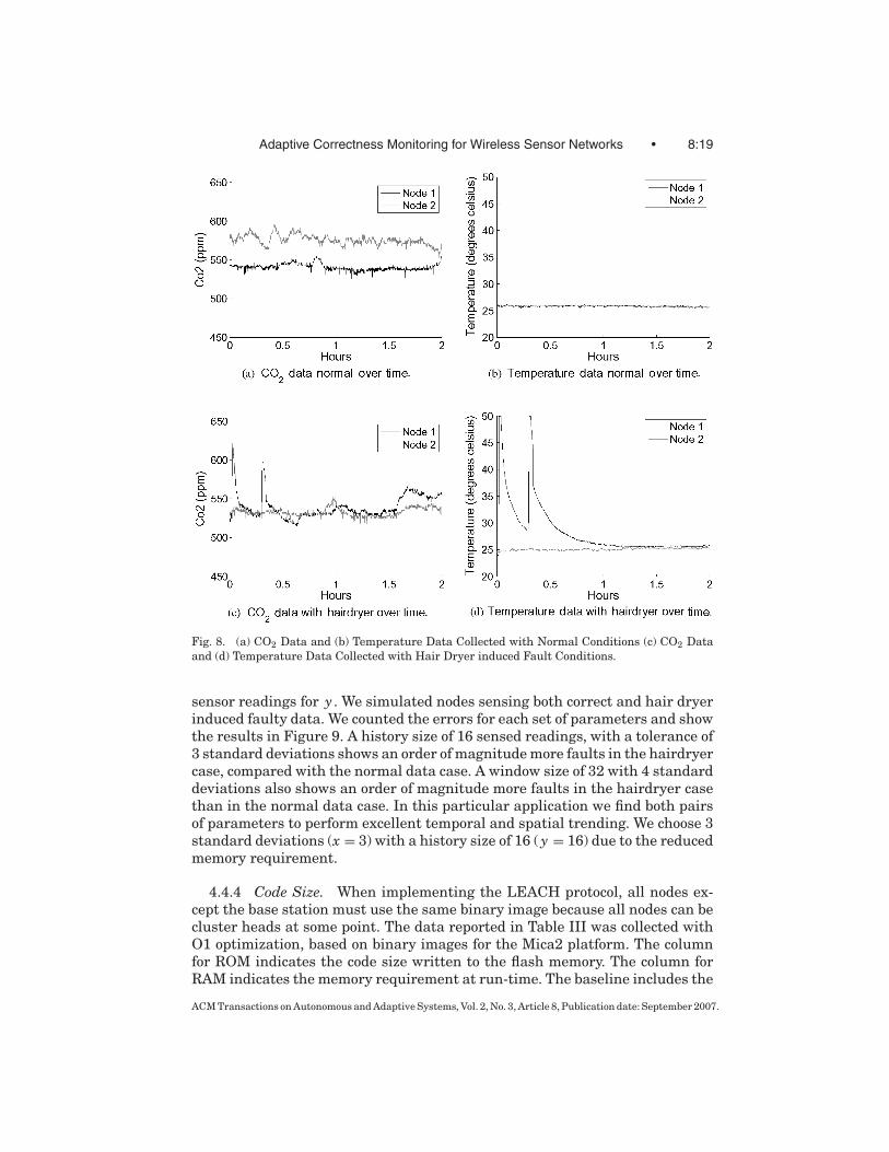
To demonstrate a real world example of choosing the proper tolerance andhistory size, we collected data from two CO2 and temperature sensors placedon different sides of an approximately 50 square meter lab with two occupantsfor 2 hours under normal air conditions. Care was taken not to perturb theenvironment. Normal building ventilation was present, and the single door tothe hallway was left open to simulate normal conditions. Data were sampledevery 30 seconds, and the base station logged the data to permanent storageduring collection. We repeated the data collection with a student temporarilyholding a 1500 Watt personal hair dryer to one node at two different times dur-ing the experiment. The hair dryer causes a quick spike in temperature to 50degrees Celsius, the maximum temperature the sensor can measure. Addition-ally, we recorded an increase in CO2 level when the student was operating thehair dryer, from the increase in air flow over the sensor and the close proximityof the student. We use this data collected with the hair dryer to represent amalfunctioning sensor or a sudden change of the environment. The CO2 andtemperature data of both the normal case, and the hair dryer case are shownin Figure 8.

To evaluate trending performance across a wide range of tolerances andhistory sizes, we inserted this data into a TOSSIM simulation, where nodes usethe data as their sensed values in a 20 node simulation of a network running theLEACH protocol. TOSSIM allows us to use the same sensed data in multiplesimulations of different tolerance and history values. The sensed data fromnode 1 simulated the sensed data for one node, the data from node 2 simulatedsensed data for 18 other nodes, and the remaining node served as the basestation. We inserted run-time determined invariants into the application codeto perform trending on (1) the time between cluster elections, (2) the number ofmembers in an individual cluster, (3) the number of clusters, (4) the number ofbytes transmitted between elections, (5) the value of the sensed CO2 data, and(6) the value of the sensed temperature data.

To determine the appropriate tolerance for spatial trending, we simulated anetwork performing spatial trending with tolerances of 1, 2, 3, 4, and 5 stan-dard deviations for the value of x with both the normal data, and the hairdryer data representing faults. We record the number of faults that were de-tected by trend monitoring, and show the results in Figure 9. At a toleranceof 4 standard deviations no errors are reported for correct data, and 310 er-rors are reported for the hair dryer simulated fault data. We can see from thefigure that a tolerance value lower than 4 shows a similar number of errorsin both the correct data and hair dryer data. Tolerances larger than 4 stan-dard deviations do not detect the errors in faulty data, and are therefore tooloose.

To determine the appropriate tolerance and history size for temporal trend-ing, we simulated a network performing temporal trending with tolerancesfrom 1 to 5 standard deviations for x, and with history sizes of 4, 8, 16, and 32



Fig. 8. (a) CO2 Data and (b) Temperature Data Collected with Normal Conditions (c) CO2 Dataand (d) Temperature Data Collected with Hair Dryer induced Fault Conditions.

sensor readings for y . We simulated nodes sensing both correct and hair dryerinduced faulty data. We counted the errors for each set of parameters and showthe results in Figure 9. A history size of 16 sensed readings, with a tolerance of3 standard deviations shows an order of magnitude more faults in the hairdryercase, compared with the normal data case. A window size of 32 with 4 standarddeviations also shows an order of magnitude more faults in the hairdryer casethan in the normal data case. In this particular application we find both pairsof parameters to perform excellent temporal and spatial trending. We choose 3standard deviations (x = 3) with a history size of 16 ( y = 16) due to the reducedmemory requirement.

4.4.4 Code Size. When implementing the LEACH protocol, all nodes ex-cept the base station must use the same binary image because all nodes can becluster heads at some point. The data reported in Table III was collected withO1 optimization, based on binary images for the Mica2 platform. The columnfor ROM indicates the code size written to the flash memory. The column forRAM indicates the memory requirement at run-time. The baseline includes the



Fig. 9. Number of faults for different sigma on normal and erroneous data, (a) Temporal Trending,(b) Spatial Trending.

Table III. Code Size of H-SEND in Bytes

Components ROM Size RAM SizeLEACH without observation 11744 1466LEACH with node level 12838 1470observationLEACH with node, and 12906 1530cluster level observationLEACH with node, cluster, and 13040 1639base station level observation

program that performs the basic sensor functionality and LEACH leader elec-tion. Adding node level observation increases the code size by 9% ( 12838

11744 − 1).Adding all levels of observation increases the code size by 11% ( 13040

11744 − 1). Theincreased RAM size comes from the additional bytes in the buffers for eachpacket.



5. CONCLUSION AND FUTURE WORK

This article presents a hierarchical approach for detecting software faults forWSNs. The detection is divided into multiple levels: node, cluster, and basestation. Programmers specify the conditions (called invariants) that have tobe satisfied. Correct values can be specified in source code and determined atcompile-time, or trending can be used to determine correct value ranges at run-time. It is possible to automatically insert invariants by a compiler. Our methodis distributed and has low overhead in code size and network traffic. Our methodcan be applied to a wide range of protocols. We use a leader election protocol asa case study, and show run-time trending on CO2 and temperature data. TheH-SEND approach is designed to be tied into other existing technologies. Forfuture work, we will address ways of detecting scenarios that trend monitor-ing cannot detect, such as sensor calibration shifting. We plan to implementautomatic invariant insertion by a compiler.

REFERENCES

AN HUANG, Y. AND LEE, W. 2003. A cooperative intrusion detection system for ad hoc networks.In ACM Workshop on Security of Ad Hoc and Sensor Networks. 135–147.

BUCHEGGER, S. AND BOUDEC, J.-Y. L. 2002. Performance analysis of the CONFIDANT protocol. InACM International Symposium on Mobile Ad Hoc Networking & Computing. 226–236.

DIAZ, M., JUANOLE, G., AND COURTIAT, J.-P. 1994. Observer—A concept for formal on-line validationof distributed systems. IEEE Trans. Softw. Engin. 20, 12.

DOLEV, S., ISRAELI, A., AND MORAN, S. 1997. Uniform dynamic self-stabilizing leader election. IEEETrans. Para. Distrib. Syst. 8, 4 (Apr.), 424–440.

EMMERICH, S. 1996. Demand-controlled ventilation in a multi-zone office building. Fuel and En-ergy Abstracts 37, 4, 294–294.

ERDMANN, C. A., STIENER, K. C., AND APTE, M. G. 2002. Indoor carbon dioxide concentrationsand sick building syndrome symptoms in the base study revisited: Analysis of the 100 buildingdataset. In Indoor Air. 443–448.

ERNST, M. D., COCKRELL, J., GRISWOLD, W. G., AND NOTKIN, D. 2001. Dynamically discovering likelyprogram invariants to support program evolution. IEEE Trans. Softw. Engin. 27, 2 (Feb.), 99–123.

GOLDSMITH, S., O’CALLAHAN, R., AND AIKEN, A. 2005. Relational queries over program traces. InACM SIGPLAN Conference on Object Oriented Programming Systems Languages and Applica-tions. 385–402.

HAGHIGHAT, F. AND DONNINI, G. 1992. IAQ and energy-management by demand controlled venti-lation. Environ. Techno. 13, 4, 351–359.

HAMLET, D. 2005. Invariants and state in testing and formal methods. In ACM SIGPLAN-SIGSOFT Workshop on Program Analysis for Software Tools and Engineering. 48–51.

HANGAL, S. AND LAM, M. S. 2002. Tracking down software bugs using automatic anomaly detec-tion. In International Conference on Software Engineering. 291–301.

HEINZELMAN, W. B., CHANDRAKASAN, A. P., AND BALAKRISHNAN, H. 2002. An application-specific pro-tocol architecture for wireless microsensor networks. IEEE Trans. Wireless Comm. 1, 4 (Oct.),660–670.

HEINZELMAN, W. R., CHANDRAKASAN, A., AND BALAKRISHNAN, H. 2000. Energy-efficient communica-tion protocol for wireless microsensor networks. In Hawaii International Conference on SystemSciences. 2, 1–10.

HERBERT, D., LU, Y.-H., BAGCHI, S., AND LI, Z. 2006. Detection and repair of software errors inhierarchical sensor networks. In IEEE International Conference on Sensor Networks, Ubiquitous,and Trustworthy Computing. 403–410.

HERBERT, D., MODELO-HOWARD, G., PEREZ-TORO, C., AND BAGCHI, S. 2007. Fault tolerant ARIMA-based aggregation of data in sensor networks. IEEE International Conference on DependableSystems and Networks.



HERBERT, D., SUNDARAM, V., ALBIN, L., LU, Y.-H., BAGCHI, S., AND LI, Z. 2007. Pervasive carbon diox-ide and temperature monitoring utilizing large numbers of low-cost wireless sensors. AmericanIndustrial Hygiene Conference and Expo. 163.

HILL, J. L. AND CULLER, D. E. 2002. Mica: A wireless platform for deeply embedded networks.IEEE Micro. 22, 6 (Nov.-Dec.), 12–24.

HUI, J. W. AND CULLER, D. 2004. The dynamic behavior of a data dissemination protocol for net-work programming at scale. In International Conference on Embedded Networked Sensor Sys-tems. 81–94.

KHALIL, I., BAGCHI, S., AND NINA-ROTARU, C. 2005. DICAS: Detection, diagnosis, and isolation ofcontrol attacks in sensor networks. In International Conference on Security and Privacy forEmerging Areas in Communications Networks. 89–100.

KHALIL, I., BAGCHI, S., AND SHROFF, N. B. 2005. LITEWORP: A Lightweight Countermeasure forthe Wormhole Attack in Multihop Wireless Networks. In IEEE International Conference on De-pendable Systems and Networks. 612–621.

KHALIL, I., BAGCHI, S., AND SHROFF, N. B. 2006. MOBIWORP: Mitigation of the wormhole attack inmobile multihop wireless networks. In IEEE International Conference on Security and Privacyin Communication Networks.

KHANNA, G., VARADHARAJAN, P., AND BAGCHI, S. 2004. Self checking network protocols: A monitorbased approach. In International Symposium on Reliable Distributed Systems. 18–30.

KUMAR, N., CHILDERS, B. R., AND SOFFA, M. L. 2005. Low overhead program monitoring and pro-filing. In ACM SIGPLAN-SIGSOFT Workshop on Program Analysis for Software Tools and En-gineering. 28–34.

LAMPORT, L., SHOSTAK, R., AND PEASE, M. 1982. The byzantine generals problem. ACM Trans.Program. Lang. Syst. 4, 3 (July), 382–401.

Levis, P., Lee, N., Welsh, M., and Culler, D. 2003. TOSSIM: Accurate and scalable simulation ofentire tinyOS applications. In International Conference on Embedded Networked Sensor Systems.126–137.

LIAO, C.-M., CHANG, C.-F., AND LIANG, H.-M. 2005. A probabilistic transmission dynamic model toaccess indoor airborne infection risks. Risk Analysis. 25, 5, 1097–1107.

LINDSEY, S., RAGHAVENDRA, C., AND SIVALINGAM, K. M. 2002. Data gathering algorithms in sen-sor networks using energy metrics. IEEE Trans. Paral. and Distrib. Syst. 13, 9 (Sept.), 924–935.

LYNCH, N. A. 1996. Distributed Algorithms. Morgan Kaufmann.MAHANEY, S. R. AND SCHNEIDER, F. B. 1985. Inexact agreement: Accuracy, precision, and graceful

degradation. ACM Symposium on Principles of Distributed Computing. 237–249.MARTI, S., GIULI, T. J., LAI, K., AND BAKER, M. 2000. Mitigating routing misbehavior in mo-

bile ad hoc networks. In International Conference on Mobile Computing and Networking. 255–265.

MARZULLO, K. 1990. Tolerating failures of continuous-valued sensors. ACM Trans. Comput. Syst.,8, 4 (Nov.), 284–304.

MEDIDI, S. R., MEDIDI, M., AND GAVINI, S. 2003. Detecting packet-dropping faults in mobile ad-hocnetworks. In IEEE ASILOMAR Conference on Signals, Systems and Computers.

MILTON, D. K., GLENCROSS, P. M., AND WALTERS, M. D. 2000. Risk of sick leave associated withoutdoor air supply rate, humidification, and occupant complaints. Indoor Air 10, 4 (Dec.), 212–221.

MIN, R., BHARDWAJ, M., CHO, S.-H., SHIH, E., SINHA, A., WANG, A., AND CHANDRAKASAN, A. 2001. Low-power wireless sensor networks. In International Conference on VLSI Design. 205–210.

MURUGANATHAN, S. D., MA, D. C. F., BHASIN, R. I., AND FAPOJUWO, A. O. 2005. A centralized energy-efficient routing protocol for wireless sensor networks. IEEE Commun. Mag. 43, 3 (Mar.), 8–13.

MYATT, T. A., JOHNSTON, S. L., ZUO, Z., WAND, M., KEBADZE, T., RUDNICK, S., AND MILTON, D. K. 2004.Detection of airborne rhinovirus and its relation to outdoor air supply in office environments.Amer. J. Respir. Critic. Care Med. 169, 1187–1190.

NAKANO, K. AND OLARIU, S. 2002. A survey on leader election protocols for radio networks. InInternational Symposium on Parallel Architectures, Algorithms and Networks. 63–68.

NASIPURI, A., CASTANEDA, R., AND DAS, S. R., 2001. Performance of multipath routing for on-demandprotocols in mobile ad hoc networks. Mobile Netw. Appl. 6, 4, 339–349.



PERKINS, J. H. AND ERNST, M. D. 2004. Efficient incremental algorithms for dynamic detectionof likely invariants. In ACM SIGSOFT International Symposium on Foundation of SoftwareEngineering. 23–32.

PIRZADA, A. A. AND MCDONALD, C. Establishing trust in pure ad hoc networks. In Conference onAustralasian Computer Science.

RAMANATHAN, N., CHANG, K., KAPUR, R., GIROD, L., KOHLER, E., AND ESTRIN, D. 2005. Sympathyfor the sensor network debugger. In International Conference On Embedded Networked SensorSystems. 255–267.

RUDNICK, S. N. AND MILTON, D. K. 2003. Risk of indoor airborne infection transmission estimatedfrom carbon dioxide concentration. Indoor Air 13, 3 (Sept.), 237–245.

SEPPANEN, O. A., FISK, W. J., AND MENDELL, M. J. 1999. Association of ventilation rates and CO2concentrations with health and other responses in commercial and institutional buildings. IndoorAir. 226–252.

SINGH, G. 1996. Leader election in the presence of link failures. IEEE Trans. Paral. Distrib. Syst.7, 3 (March), 231–236.

SMITH, B. R., MURTHY, S., AND GARCIA-LUNA-ACEVES, J. J. 1997. Securing distance-vector routingprotocols. In Proceedings of the Symposium on Network and Distributed System Security. 85–92.

SORO, S. AND HEINZELMAN, W. B. 2005. Prolonging the lifetime of wireless sensor networks viaunequal clustering. In IEEE International Parallel and Distributed Processing Symposium, page236b.

TEL, G. 1991. Topics in Distributed Algorithms. Cambridge University Press, Chapter 3: Asser-tional Verification.

VIGNA, G., GWALANI, S., SRINIVASAN, K., BELDING-ROYER, E. M., AND KEMMERER, R. A. 2004. An intru-sion detection tool for AODV-based ad hoc wireless networks. In IEEE Annual Computer SecurityApplications Conference.

WANG, J. YI., SHUE, Y.-S., VIJAYKUMAR, T. N., AND BAGCHI, S. 2006. Pesticide: Using SMT processorsto improve performance of pointer bug detection. In IEEE International Conference on ComputerDesign.

YEN, I.-L., BASTANI, F. B., AND TAYLOR, D. J. 2001. Design of multi-invariant data structures forrobust shared accesses in multiprocessor systems. IEEE Trans. Softw. Engin. 27, 3, 193–207.

YOUNIS, M., YOUSSEF, M., AND ARISHA. K. Energy-aware routing in cluster-based sensor networks. InIEEE International Symposium on Modeling, Analysis and Simulation of Computer and Telecom-munications Systems. 129–136.

YU, I. T., LI, Y., WONG, T. W., TAM, W., CHAN, A. T., LEE, J. H., LEUNG, D. Y., AND HO, T. 2004. Evidenceof airborne transmission of the severe acute respiratory syndrome virus. New Engl. J. Med. 350,17 (Apr.), 1731–1739.

ZHOU, Y., ZHOU, P., QIN, F., LIU, W., AND TORRELLAS, J. 2005. Efficient and flexible architecturalsupport for dynamic monitoring. ACM Trans. Arch. Code Optim. 2, 1 (March), 3–33.

ZULKERNINE M. AND SEVIORA, R. E. 2002. A Compositional approach to monitoring distributedsystems. In International Conference on Dependable Systems and Networks. 763–772.

Received March 2006; revised November 2006; accepted May 2007


Adaptive Correctness Monitoring for Wireless Sensor Networks Using Hierarchical ...€¦ · ·...

Documents

Transcript of Adaptive Correctness Monitoring for Wireless Sensor Networks Using Hierarchical ...€¦ · ·...