Adaptive Blind Channel Equalizationww3.comsats.edu.pk/faculty/users/ee/sabrar/abrar_third.pdf ·...

0

Adaptive Blind Channel Equalization

Shafayat Abrar1, Azzedine Zerguine2 and Asoke Kumar Nandi31Department of Electrical Engineering,

COMSATS Institute of Information Technology, Islamabad 440002Department of Electrical Engineering,

King Fahd University of Petroleum and Minerals, Dhahran 312613Department of Electrical Engineering and Electronics,

The University of Liverpool, Liverpool L69 3BX1Pakistan

2Saudi Arabia3United Kingdom

1. Introduction

For bandwidth-efficient communication systems, operating in high inter-symbol interference(ISI) environments, adaptive equalizers have become a necessary component of the receiverarchitecture. An accurate estimate of the amplitude and phase distortion introduced by thechannel is essential to achieve high data rates with low error probabilities. An adaptiveequalizer provides a simple practical device capable of both learning and inverting thedistorting effects of the channel. In conventional equalizers, the filter tap weights are initiallyset using a training sequence of data symbols known both to the transmitter and receiver.These trained equalizers are effective and widely used. Conventional least mean square (LMS)adaptive filters are usually employed in such supervised receivers, see Haykin (1996).

However, there are several drawbacks to the use of training sequences. Implementing atraining sequence can involve significant transceiver complexity. Like in a point-to-multipointnetwork transmissions, sending training sequences is either impractical or very costly interms of data throughput. Also for slowly varying channels, an initial training phasemay be tolerable. However, there are scenarios where training may not be feasible, forexample, in equalizer implementations of digital cellular handsets. When the communicationsenvironment is highly non-stationary, it may even become grossly impractical to use trainingsequences. A blind equalizer, on the other hand, does not require a training sequenceto be sent for start-up or restart. Rather, the blind equalization algorithms use a prioriknowledge regarding the statistics of the transmitted data sequence as opposed to an exactset of symbols known both to the transmitter and receiver. In addition, the specifications oftraining sequences are often left ambiguous in standards bodies, leading to vendor specifictraining sequences and inter-operability problems. Blind equalization solves this problem aswell, see Ding & Li (2001); Garth et al. (1998); Haykin (1994).

In this Chapter, we provide an introduction to the basics of adaptive blind equalization.We describe popular methodologies and criteria for designing adaptive algorithms for blind

2 Digital Communication

equalization. Most importantly, we discuss how to use the probability density function(PDF) of transmitted signal to design ISI-sensitive cost functions. We discuss the issues ofadmissibility of proposed cost function and stability of derived adaptive algorithm.

2. Trained and blind adaptive equalizers: Historical persp ectives

Adaptive trained channel equalization was first developed by Lucky for telephone channels,see Lucky (1965; 1966). Lucky proposed the so-called zero-forcing (ZF) method to be appliedin FIR equalization. It was an adaptive procedure and in a noiseless situation, the optimalZF equalizer tends to be the inverse of the channel. In the mean time, Widrow and Hoffintroduced the least mean square (LMS) adaptive algorithm which begins adaptation with theaid of a training sequence known to both transmitter and receiver, see Widrow & Hoff (1960);Widrow et al. (1975). The LMS algorithm is capable of reducing mean square error (MSE)between the equalizer output and the training sequence. Once the signal eye is open, theequalizer is then switched to tracking mode which is commonly known as decision-directedmode. The decision-directed method is unsupervised and its effectiveness depends on theinitial condition of equalizer coefficients; if the initial eye is closed then it is likely to diverge.

In blind equalization, the desired signal is unknown to the receiver, except for its probabilisticor statistical properties over some known alphabets. As both the channel and its input areunknown, the objective of blind equalization is to recover the unknown input sequencebased solely on its probabilistic and statistical properties, see C.R. Johnson, Jr. et al. (1998);Ding & Li (2001); Haykin (1994). Historically, the possibility of blind equalization was firstdiscussed in Allen & Mazo (1974), where the authors proved analytically that an adjustingequalizer, optimizing the mean-squared sample values at its output while keeping a particulartap anchored at unit value, is capable of inverting the channel without needing a trainingsequence. In the subsequent year, Sato was the first who came up with a robust realization ofan adaptive blind equalizer for PAM signals, see Sato (1975). It was followed by a number ofsuccessful attempts on blind magnitude equalization (i.e., equalization without carrier-phaserecovery) in Godard (1980) for complex-valued signals (V29/QPSK/QAM), in Treichler &Agee (1983) for AM/FM signals, in Serra & Esteves (1984) and Bellini (1986) for PAM signals.However, many of these algorithms originated from intuitive starting points.

The earliest works on joint blind equalization and carrier-phase recovery were reported inBenveniste & Goursat (1984); Kennedy & Ding (1992); Picchi & Prati (1987); Wesolowski(1987). Recent references include Abrar & Nandi (2010a;b;c;d); Abrar & Shah (2006a); Abrar &Qureshi (2006b); Abrar et al. (2005); Goupil & Palicot (2007); Im et al. (2001); Yang et al. (2002);Yuan & Lin (2010); Yuan & Tsai (2005). All of these blind equalizers are capable of recoveringthe true power of transmitted data upon convergence and are classified as Bussgang-type, seeBellini (1986). The Bussgang blind equalization algorithms make use of a nonlinear estimateof the channel input. The memoryless nonlinearity, which is the function of equalizer output,is designed to minimize an ISI-sensitive cost function that implicitly exploits higher-orderstatistics. The performance of such kind of blind equalizer depends strongly on the choice ofnonlinearity.

The first comprehensive analytical study of the blind equalization problem was presentedby Benveniste, Goursat, and Ruget in Benveniste et al. (1980a;b). They established that ifthe transmitted signal is composed of non-Gaussian, independent and identically distributed

Adaptive Blind Channel Equalization 3

samples, both channel and equalizer are linear time-invariant filters, noise is negligible, andthe probability density functions of transmitted and equalized signals are equal, then thechannel has been perfectly equalized. This mathematical result is very important since itestablishes the possibility of obtaining an equalizer with the sole aid of signal’s statisticalproperties and without requiring any knowledge of the channel impulse response or trainingdata sequence. Note that the very term “blind equalization” can be attributed to Benvenisteand Goursat from the title of their paper Benveniste & Goursat (1984). This seminal paperestablished the connection between the task of blind equalization and the use of higher-orderstatistics of the channel output. Through rigorous analysis, they generalized the original Satoalgorithm into a class of algorithms based on non-MSE cost functions. More importantly, theconvergence properties of the proposed algorithms were carefully investigated.

The second analytical landmark occurred in 1990 when Shalvi and Weinstein significantlysimplified the conditions for blind equalization, see Shalvi & Weinstein (1990). Before thiswork, it was usually believed that one needs to exploit infinite statistics to ensure zero-forcingequalization. Shalvi and Weinstein showed that the zero-forcing equalization can be achievedif only two statistics of the involved signals are restored. Actually, they proved that, ifthe fourth order cumulant (kurtosis) is maximized and the second order cumulant (energy)remains the same, then the equalized signal would be a scaled and rotated version of thetransmitted signal. Interesting accounts on Shalvi and Weinstein criterion can be found inTugnait et al. (1992) and Romano et al. (2011).

3. System model and “Bussgang” blind equalizer

The baseband model for a typical complex-valued data communication system consists of anunknown linear time-invariant channel {h} which represents the physical inter-connectionbetween the transmitter and the receiver. The transmitter generates a sequence ofcomplex-valued random input data {an}, each element of which belongs to a complexalphabet A. The data sequence {an} is sent through the channel whose output xn is observedby the receiver. The input/output relationship of the channel can be written as:

xn = ∑k

an−khk + νn, (1)

where the additive noise νn is assumed to be stationary, Gaussian, and independent of thechannel input an. We also assume that the channel is stationary, moving-average and hasfinite length. The function of equalizer at the receiver is to estimate the delayed version

of original data, an−δ, from the received signal xn. Let wn = [wn,0, wn,1, · · · , wn,N−1]T

be vector of equalizer coefficients with N elements (superscript T denotes transpose). Let

xn = [xn, xn−1 · · · , xn−N+1]T be the vector of channel observations. The output of the

equalizer isyn = w

Hn xn (2)

where superscript H denotes conjugate transpose. If {t} = {h} ⋆ {w∗} represents the overallchannel-equalizer impulse response (where ⋆ denotes convolution), then (2) can be expressed


as:

yn = ∑i w∗i xn−i = ∑l an−ltl + ν

′n = tδ an−δ + ∑

l 6=δ

tl an−l + ν′n

︸︷︷︸signal + ISI + noise

(3)

Equation (3) distinctly exposes the effects of multi-path inter-symbol interference and additivenoise. Even in the absence of additive noise, the second term can be significant enough tocause an erroneous detection.

The idea behind a Bussgang blind equalizer is to minimize (or maximize), through thechoice of equalizer filter coefficients w, a certain cost function J, depending on the equalizeroutput yn, such that yn provides an estimate of the source signal an up to some inherentindeterminacies, giving, yn = α an−δ, where α = |α|eγ ∈ C represents an arbitrary gain. Thephase γ represents an isomorphic rotation of the symbol constellation and hence is dependenton the rotational symmetry of signal alphabets; for example, γ = mπ/2 radians, withm ∈ {0, 1, 2, 3} for a quadrature amplitude modulation (QAM) system. Hence, a Bussgangblind equalizer tries to solve the following optimization problem:

w† = arg optimizew J, with J = E[J (yn)] (4)

The cost J is an expression for implicitly embedded higher-order statistics of yn and J (yn) is areal-valued function. Ideally, the cost J makes use of statistics which are significantly modifiedas the signal propagates through the channel, and the optimization of cost modifies thestatistics of the signal at the equalizer output, aligning them with those at channel input. Theequalization is accomplished when equalized sequence yn acquires an identical distributionas that of the channel input an, see Benveniste et al. (1980a). If the implementation method isrealized by stochastic gradient-based adaptive approach, then the updating algorithm is

wn+1 = wn ± µ

(∂J∂wn

)∗(5a)

= wn + µΦ(yn)∗xn, with Φ(yn) = ± ∂J

∂y∗n(5b)

where µ is step-size, governing the speed of convergence and the level of steady-stateperformance, see Haykin (1996). The positive and negative signs in (5a) are respectivelyfor maximization and minimization. The complex-valued error-function Φ(yn) can beunderstood as an estimate of the difference between the desired and the actual equalizeroutputs. That is, Φ(yn) = Ψ(yn)− yn, where Ψ(yn) is an estimate of the transmitted data an.The nonlinear memory-less estimate, Ψ(yn), is usually referred to as Bussgang nonlinearityand is selected such that, at steady state, when yn is close to an−δ, the autocorrelation of yn

becomes equal to the cross-correlation between yn and Ψ(yn), i.e.,

E [ynΦ(yn−i)∗] = 0 ⇒ E

[yn y∗n−i

]= E [ynΨ(yn−i)

∗]

An admissible estimate of Ψ(yn), however, is the conditional expectation E [an′ |yn], seeNikias & Petropulu (1993). Using Bayesian estimation technique, E [an′ |yn] was derived in


Bellini (1986); Fiori (2001); Haykin (1996); Pinchas & Bobrovsky (2006; 2007). These methods,however, rely on explicit computation of higher-order statistics and are not discussed here.

4. Trained and blind equalization design methodologies

Generally, a blind equalization algorithm attempts to invert the channel using both thereceived data samples and certain known statistical properties of the input data. For example,it is easy to show that for a minimum phase channel, the spectra of the input and outputsignals of the channel can be used to determine the channel impulse response. However,most communication channels do not possess minimum phase. To identify a non-minimumphase channel, a non-Gaussian signal is required along with nonlinear processing at thereceiver using higher-order moments of the signal, see Benveniste et al. (1980a;b). Basedupon available analysis, simulations, and experiments in the literature, it can be said thatan admissible blind cost function has two main attributes: 1) it makes use of statistics whichare significantly modified as the signal propagates through the channel, and 2) optimizationof the cost function modifies the statistics of the signal at the channel output, aligning themwith the statistics of the signal at the channel input.

Designing a blind equalization cost function has been lying strangely more in the realm ofart than science; majority of the cost functions tend to be proposed on intuitive groundsand then validated. Due to this reason, a plethora of blind cost functions is available inliterature. On the contrary, the fact is that there exist established methods which facilitate thedesigning of blind cost functions requiring statistical properties of transmitted and receivedsignals. One of the earliest methods originated in late 70’s in geophysics community whosought to determine the inverse of the channel in seismic data analysis and it was namedminimum entropy deconvolution (MED), see Gray (1979b); Wiggins (1977). Later in early90’s, Satorius and Mulligan employed MED principle and came up with several proposals toblindly equalize the communication channels, see Satorius & Mulligan (1993). However, thosemarvelous signal-specific proposals regrettably failed to receive serious attention.

In the sequel, we discuss MED along with other popular methods for designing blind costfunctions and corresponding adaptive equalizers.

4.1 Lucky criterion

In 1965, Lucky suggested that the propagation channel may be inverted by an equalizer ifequalizer minimizes the following peak distortion criterion, see Lucky (1965):

Jpeak =1

|tδ| ∑l 6=δ

|tl | (6)

This criterion is equivalent to requiring that the equalizer maximizes the eye opening. theintuitive explanation of (6) is as follows. From (3), ignoring the noise, obtain the value of errorE due to ISI, given as E = yn − an−δ = an−δ (tδ − 1) + ∑l 6=δ tl an−l . Assuming the maximumand minimum values of an are a and −a, respectively; the maximum error is easily written as

Emax = |yn − an−δ|max = |an−δ| |tδ − 1|+ a ∑l 6=δ

|tl | (7)


If tδ is close to unity, then the cost Jpeak is the scaled version of Emax as given by Jpeak ≈Emax/(|tδ|a). It is important to note that the cost Jpeak is a convex function of the equalizerweights and has a well-defined minimum. Thus any minimum of Jpeak found by gradientsearch or other systematic programming methods must be the absolute (or global) minimumof distortion, see Lucky (1966). To prove the convexity of Jpeak, it is necessary to show that for

two equalizer settings w(a) and w(b) and for all η, 0 ≤ η ≤ 1

Jpeak(η w(a) + (1 − η)w(b)) ≤ η Jpeak(w

(a)) + (1 − η)Jpeak(w(b)) (8)

The above equation shows that the distortion always lies on or beneath the chord joiningvalues of distortion in N-spaces. Below is the proof of (8):

Jpeak(η w(a) + (1 − η)w(b)) = ∑

l 6=δ

∣∣∣∣∑k

hk

(η (w

(a)l−k)

∗ + (1 − η)(w(b)l−k)

∗)∣∣∣∣

≤ η ∑l 6=δ

∣∣∣∣∑k

hk(w(a)l−k)

∗∣∣∣∣+ (1 − η) ∑

l 6=δ

∣∣∣∣∑k

hk(w(b)l−k)

∗∣∣∣∣

= η Jpeak(w(a)) + (1 − η)Jpeak(w

(b)).

(9)

However, in practice, it is not an easy one to achieve this convexity in a gradient search(adaptive) procedure, as it is necessary to obtain the projection of the gradient onto theconstraint hyperplane, see Allen & Mazo (1973). Alternatively one can also seek to minimizethe mean-square distortion criterion:

Jms =1

|tδ|2 ∑l 6=δ

|tl |2 (10)

The cost Jms is not convex but unimodal, mathematically tractable and capable of yieldingadmissible solution, see Allen & Mazo (1973). Under the assumption |tδ| = max{|t|}, Shalvi& Weinstein (1990) used the expression (10) to quantify ISI, i.e., ISI = Jms. Using criterion (10),we can formulate the following tractable problem for ISI mitigation:

w† = arg min

w∑l 6=δ

|tl |2 s.t. |tδ| = 1. (11)

where we have assumed that the equalizer coefficients (w†) have been selected such that thecondition (|tδ| = 1) is always satisfied. Introducing the channel autocorrelation matrix H,whose (i, j) element is given by Hij = ∑k hk−ih

∗k−j, we can show that ∑l |tl |2 = wH

n Hwn. The

equalizer has to make one of the coefficients of {tl} say tδ = t0 = wHn h to be unity and others

to be zero, where h = [hK−1, hK−2, · · · , h1, h0]T; it gives the value of ISI of an unequalized

system at time index n as follows:

ISI =wH

n Hwn

|wHn h|2 − 1. (12)


Now consider the optimization of the problem (11). Using Lagrangian multiplier λ, we obtain

∑l 6=δ

|tl|2 + λ (tδ − 1) = wHn Hwn − 1 + λ

(w

Hn h − 1

)(13)

Next differentiating with respect to w∗n and equating to zero, we get Hwn + λh = 0 ⇒ wn =

−λH−1h. Substituting the above value of wn in (12), we obtain

ISIn =h

HH

−1h

|hHH

−1h|2

− 1. (14)

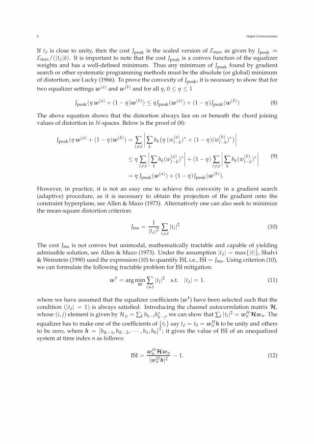
To appreciate the possible benefit of solution (14), consider a channel h−1 = 1 − ε, h0 = ε andh1 = 0, where 0 ≤ ε ≤ 1. Without equalizer, we have

ISI =(1 − ε)2 + ε2

max(1 − ε, ε)2− 1. (15)

The ISI approaches zero when ε is either zero or unity. Assuming a 2-tap equalizer, we obtain

H =

[(1 − ε)2 + ε2 (1 − ε)ε(1 − ε)ε (1 − ε)2 + ε2

](16)

Using (14) and (16), we obtain

ISI =ε2(1 − ε)2

1 − 4ε + 6ε2 − 4ε3 + 2ε4. (17)

Refer to Fig. 1, the ISI (17) of the equalized system is lower than that of the uncompensatedsystem. The adaptive implementation of Jms can be realized in a supervised scenario.

0 0.1 0.2 0.3 0.4 0.5 0.6 0.7 0.8 0.9 10

0.2

0.4

0.6

0.8

1

ε

ISI

EqualizedUnequalized

Fig. 1: ISI of unequalized and equalized systems.

Combining the two expression (7) and (10), the following cost is obtained which is usuallytermed as mean square error (MSE) criterion, see Widrow et al. (1975):

Jmse = E

[∣∣an−δ − yn

∣∣2]

(18)


Minimizing (18), we obtain the following update:

wn+1 = wn + µ (an−δ − yn)∗

xn, (19)

which is known as LMS algorithm or Widrow-Hoff algorithm. Note that the parameter µ is apositive step-size and the following value of µ ≡ µLMS ensures the stability of algorithm, seeFarhang-Boroujeny (1998):

0 < µLMS <1

2NPa, (20)

where Pa = E[|a|2]

is the average energy of signal an and N is the length of equalizer.

4.2 Minimum entropy deconvolution criterion

The minimum entropy deconvolution (MED) is probably the earliest principle for designingcost functions for blind equalization. This principle was introduced by Wiggins in seismic dataanalysis in the year 1977, who sought to determine the inverse channel w† that maximizes thekurtosis of the deconvolved data yn, see Wiggins (1977; 1978). For seismic data, which aresuper-Gaussian in nature, he suggested to maximize the following cost:

1B ∑

Bb=1 |yn−b+1|4(

1B ∑

Bb=1 |yn−b+1|2

)2(21)

This deconvolution scheme seeks the smallest number of large spikes consistent with the data,thus maximizing the order or, equivalently, minimizing the entropy or disorder in the data,Walden (1985). Note that the equation (21) has the statistical form of sample kurtosis and theexpression is scale-invariant. Later, in the year 1979, Gray generalized the Wiggins’ proposalwith two degrees of freedom as follows, Gray (1979b):

J(p,q)med ≡

1B ∑

Bb=1 |yn−b+1|p

(1B ∑

Bb=1 |yn−b+1|q

) pq

(22)

The criterion was rigorously investigated in Donoho (1980), where Donoho developed generalrules for designing MED-type estimators. Several cases of MED, in the context of blind

deconvolution of seismic data, have appeared in the literature, like J(2,1)med in Ooe & Ulrych

(1979), J(4,2)med in Wiggins (1977), limε→0 J

(p−ε,p)med in Claerbout (1977), J

(p,2)med in Gray (1978), and

J(2p,p)med in Gray (1979a).

In the derivation of the criterion (22), it is assumed that the original signal an, which is primaryreflection coefficients in geophysical system or transmitted data in communication systems,can be modeled as realization of independent non-Gaussian process with distribution

pA(a; α) =α

2βΓ(

1α

) exp

(− |a|α

βα

)(23)

where signal an is real-valued, α is the shape parameter, β is the scale parameter, and Γ(·)is the Gamma function. This family covers a wide range of distributions. The certain event


(α = 0), double exponential (α = 1), Gaussian (α = 2), and uniform distributions (α → ∞)are all members. For geophysical deconvolution problem, we have the range 0.6 ≤ α ≤ 1.5,and for communication system where the signals are uniformly distributed we have (α → ∞).Although, signals in communication are discrete, the equation (23) is still good to approximatesome densely and uniformly distributed signal.

In the context of geophysics, where the primary coefficient an is super-Gaussian, maximizingthe criterion (23) drives the distribution of deconvolved sequence yn away from pY (yn; p)towards pY (yn; q), where p > q. However, for the communication blind equalization problem,the underlying distribution of the transmitted (possibly pulse amplitude modulated) datasymbols are closer to a uniform density (sub-Gaussian) and thus we would minimize the cost(23) with p > q. We have the following cost for blind equalization of communication channel:

w† =

arg minw

J(p,q)med , if p > q,

arg maxw

J(p,q)med , if p < q.

(24)

The feasibility of (24) for blind equalization of digital signals has been studied in Satorius &Mulligan (1992; 1993) and Benedetto et al. (2008). In Satorius & Mulligan (1992), implementing(24) with p > q, the following adaptive algorithm was obtained:

wn+1 = wn + µB

∑k=1

(∑

Bb=1 |yn−b+1|p

∑Bb=1 |yn−b+1|q

|yn−k+1|q−2 − |yn−k+1|p−2

)y∗n−k+1 xn−k+1, (25)

In the sequel, we will refer to (25) as Satorius-Mulligan algorithm (SMA). Also, for a detaileddiscussion on the stochastic approximate realization of MED, refer to Walden (1988).

4.3 Constant modulus criterion

The most popular and widely studied blind equalization criterion is the constant moduluscriterion, Godard (1980); Treichler & Agee (1983); Treichler & Larimore (1985); it is given by

Jcm = E

[(|yn|2 − Rcm

)2]

, (26)

where Rcm = E[|a|4]/E[|a|2]

is a statistical constant usually termed as dispersion constant.For an input signal that has a constant modulus |an| =

√Rcm, the criterion penalizes output

samples yn that do not have the desired constant modulus characteristics. This modulusrestoral concept has a particular advantage in that it allows the equalizer to be adaptedindependent of carrier recovery. Because the cost is insensitive to the phase of yn, theequalizer adaptation can occur independently and simultaneously with the operation of thecarrier recovery system. This property also makes it applicable to analog modulation signalswith constant amplitude such as those using frequency or phase modulation, see Treichler& Larimore (1985). The stochastic gradient-descent minimization of (26) yields the followingalgorithm:

wn+1 = wn + µ(

Rcm − |yn|2)

y∗n xn, (27)


which is usually termed as constant modulus algorithm (CMA). Note that, considering B = 1,p = 4, q = 2 and large B, SMA (25) reduces to CMA.

If data symbols are independent and identically distributed, noise is negligible and the lengthof the equalizer is infinite then after some calculations, the CM cost may be expressed as afunction of joint channel-equalizer impulse response coefficients as follows:

Jcm =(E[|an|4]− 2E[|an|2]2

)∑

l

|tl|4 + 2E[|an|2]2(

∑l

|tl |2)2

− 2E[|an|4]∑l

|tl |2 + const.

(28)As in Godard (1980), the partial derivative of Jcm with respect to tk can be written as

∂ Jcm

∂ tk= 4tk

(E[|an|4](|tk|2 − 1) + 2E[|an|2]2 ∑

l 6=k

|tl |2)

(29)

The minimum can be found by solving ∂ Jcm

∂ tk= 0, i.e.,

tk

(E[|an|4](|tk|2 − 1) + 2E[|an|2]2 ∑

l 6=k

|tl|2)

= 0, ∀ k (30)

Unfortunately, the set of equations has an infinite number of solutions; the cost Jcm is thusnon-convex. The solutions TM, M = 1, 2, · · ·, can be represented as follows: all elementsof the set {tl} are equal to zero, except M of them and those non-zero elements have equalmagnitude of σ2

M defined by

σ2M =

E[|an|4]E[|an|4] + 2(M− 1)E[|an|2]2

(31)

Among these solutions, under the condition E[|an|4] < 2E[|an|2]2, the solution T1 is that forwhich the energy is the largest at the equalizer output and ISI is zero. The absolute minimumof Jcm is therefore reached in the case of zero IS1.

4.4 Shtrom-Fan criterion

In the year 1998, Shtrom and Fan presented a class of cost functions for achieving blindequalization which were solely the function of {t} parameters, see Shtrom & Fan (1998). Theysuggested to minimize the difference between any two norms of the joint channel-equalizerimpulse response, each raised to the same power, i.e.,

Jsf =

(

∑l

|tl |p)r/p

−(

∑l

|tl |q)r/q

, p < q and r > 0 (32)

where p, q, r ∈ ℜ. This proposal was based on the following property of vector norms:

lims→0

s√

∑l

|tl |s ≥ · · · ≥ p√

∑l

|tl|p ≥ q√

∑l

|tl |q ≥ · · · ≥ limm→∞

m√

∑l

|tl|m (33)


where p < q and equality occurs if and only if tl = ±δl−k, k ∈ Z, which is precisely thezero-forcing condition. From the above there is a multitude of cost functions to choose from.From (32), we have following possibilities to minimize:

∑l |tl | − maxl{|tl |}, (p = 1, q → ∞, r = 1) (34a)

(∑l |tl |)2 − ∑l |tl |2, (p = 1, q = r = 2) (34b)

(∑l |tl|2)2 − ∑l |tl |4, (p = 2, q = r = 4) (34c)

(∑l |tl|2)3 − ∑l |tl |6, (p = 2, q = r = 6) (34d)

(∑l |tl |4)2 − ∑l |tl|8, (p = 4, q = r = 8). (34e)

Some of these cost functions are easily implementable, whereas others are not.

Consider p = 2 and q = r = 2m in (32) to obtain a subclass:

Jsubsf =

(

∑l

|tl |2)m

− ∑l

|tl |2m (35)

This subclass is not convex, although it is potentially unimodal in t domain and easilyimplementable. As in Shtrom & Fan (1998), the partial derivative of Jsub

sf with respect to tk

can be written as

∂ Jsubsf

∂ tk= 2mtk

(

∑l

|tl |2)m−1

− |tk|2(m−1)

(36)

The equation (36) has two solutions, one of which corresponds to tl = 0, ∀l. This solutionwill not occur if a constraint is imposed. The other solution is the minimum corresponding tozero-forcing condition. This is seen from (36) as ∑l |tl|2 = |tk|2, which can only hold when t

has at most one nonzero element, i.e., the desired delta function. Now compare this result withthat of constant modulus in equation (31) which contains multiple nonzero-forcing solutions.It means, in contrast to CMA, it is less likely to have local minima in Jsub

sf in equalizer domain.

The cost functions (34a), in their current form, are not directly applicable in real scenario aswe have no information of {t}’s. These costs need to be converted from functions of {t}’s tofunctions of yn’s. As in Shtrom & Fan (1998), we can show that

∑l |tl |2 =C

yn

1,1

Ca1,1

=E[|yn|2]E[|a|2] (37a)

∑l |tl|4 =C

yn

2,2

Ca2,2

=E[|yn|4]− 2E[|yn|2]2E[|a|4]− 2E[|a|2]2 (37b)

∑l |tl |6 =C

yn

3,3

Ca3,3

=E[|yn|6]− 9E[|yn|4]E[|yn|2] + 12E[|yn|2]3

E[|a|6]− 9E[|a|4]E[|a|2] + 12E[|a|2]3 (37c)

where Czp,q is (p + q)th order cumulant of complex random variable defined as follows:

Czp,q = cumulant

(z, · · · , z︸︷︷︸

p terms

; z∗, · · · , z∗︸︷︷︸q terms

)(38)


Using (37a) and assuming m = 2, we obtain the following expression for Jsubsf :

Jsubsf =

(E[|yn|2]E[|a|2]

)2

− E[|yn|4]− 2E[|yn|2]2E[|a|4]− 2E[|a|2]2 (39)

Minimizing (39) with respect to coefficients w∗, we obtain the following adaptive algorithm:

wn+1 = wn + µ

(Rcm

PaE[|yn|2]− |yn|2

)y∗n xn, (40a)

E[|yn+1|2] = E[|yn|2] + 1n

(|yn|2 − E[|yn|2]

)(40b)

where Pa is the average energy of signal an and Rcm is the same statistical constant as wedefined in CMA. Note that the algorithm requires an iterative estimate of equalizer outputenergy. We will refer to (40) as Shtrom-Fan Algorithm (SFA).

4.5 Shalvi-Weinstein criterion

Earlier to Shtrom and Fan, in the year 1990, Shalvi and Weinstein suggested a criterion thatlaid the theoretical foundation to the problem of blind equalization, see Shalvi & Weinstein(1990). They demonstrated that the condition of equality between the PDF’s of the transmittedand equalized signals, due to BGR theorem Benveniste et al. (1980a;b), was excessively tight.Under the similar assumptions, as laid by Benveniste et al., they demonstrated that it ispossible to perform blind equalization by satisfying the condition E[|yn|2] = E[|an|2] andensuring that a nonzero cumulant of order higher than 2 of an and yn are equal.

For a two dimensional signal an with four-quadrant symmetry (i.e., E[a2n] = 0), they suggested

to maximize the following unconstrained cost function (which involved second and fourthorder cumulants):

Jsw = sgn

[Can

2,2

] (C

yn

2,2 + (γ1 + 2)(

Cyn

1,1

)2+ 2γ2 C

yn

1,1

)(41a)

= sgn

[Can

2,2

] (E

[|yn|4

]+ γ1E

[|yn|2

]2+ 2γ2E

[|yn|2

])(41b)

where γ1 and γ2 are some statistical constants. The corresponding stochastic gradientalgorithm is given by

wn+1 = wn + µ sgn[Can2,2](

γ1E[|yn|2] + |yn|2 + γ2

)y∗n xn, (42a)

E[|yn+1|2] = E[|yn|2] +1

n

(|yn|2 − E[|yn|2]

)(42b)

where (sgn[Can2,2] = −1) due to the sub-Gaussian nature of digital signals. The above

algorithm is usually termed as Shalvi-Weinstein algorithm (SWA). Note that SWA unifiesCMA and SFA (i.e., the specific case in Equation (40)). Substituting γ1 = 0 and γ2 = −Rcm

in SWA, we obtain CMA (27). Similarly, substituting γ2 = 0 and γ1 = −Rcm/Pa in SWA,we obtain SFA (40). Note that the Shtrom-Fan criterion appears to be the generalization ofShalvi-Weinstein criterion with cumulants of generic orders.


5. Blind equalization of APSK signal: Employing MED princip le

5.1 Designing a blind cost function

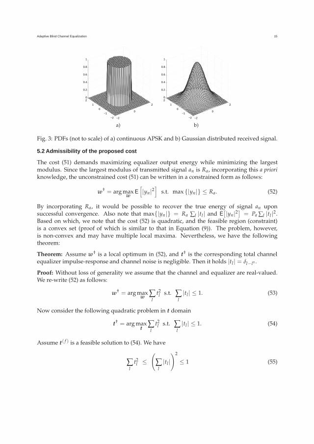
We employ MED principle and use the PDFs of transmitted amplitude-phase shift-keying(APSK) and ISI-affected received signal to design a cost function for blind equalization.Consider a continuous APSK signal, where signal alphabets {aR + aI} ∈ A are assumedto be uniformly distributed over a circular region of radius Ra and center at the origin. Thejoint PDF of aR and aI is given by (refer to Fig. 3(a))

pA(aR + aI) =

1

πR2a

,√

a2R + a2

I ≤ Ra,

0, otherwise.(43)

Now consider the transformation Y =√

a2R + a2

I and Θ = ∠(aR, aI), where Y is the modulus

and ∠() denotes the angle in the range (0, 2π) that is defined by the point (i, j). The jointdistribution of the modulus Y and Θ can be obtained as pY ,Θ(y, θ) = y/(πR2

a), y ≥ 0, 0 ≤θ < 2π. Since Y and Θ are independent, we obtain a triangular distribution for Y given bypY (y : H0) = 2y/R2

a, y ≥ 0, where H0 denotes the hypothesis that signal is distortion-free.Let Yn,Yn−1, · · · ,Yn−N+1 be a sequence, of size N, obtained by taking modulus of randomly

Ra

aI

aR

a) b)

Fig. 2: a) A continuous APSK, and b) a discrete practical 16APSK.

generated distortion-free signal alphabets A, where subscript n indicates discrete time index.Let Z1,Z2, · · · ,ZN be the order statistic of sequence {Y}. Let pY (yn, yn−1, · · · , yn−N+1 : H0)be an N-variate density of the continuous type, then, under the hypothesis H0, we obtain

pY (yn, yn−1, · · · , yn−N+1 : H0) =2N

R2Na

N

∏k=1

yn−k+1. (44)

Next we find p∗Y (yn, yn−1, · · · , yn−N+1 : H0) as follows:

p∗Y (yn , yn−1, · · · , yn−N+1 : H0) =∫ ∞

0pY (λyn, λyn−1, · · · , λyn−N+1 : H0)λ

N−1 dλ

=2N

R2Na

N

∏k=1

yn−k+1

∫ Ra/zN

0λ2N−1 dλ =

2N−1

N (zN)2N

N

∏k=1

yn−k+1,

(45)


where z1, z2, · · · , zN are the order statistic of elements yn, yn−1, · · · , yn−N+1, so that z1 =min{y} and zN = max{y}. Now consider the next hypothesis (H1) that signal suffers withmulti-path interference as well as with additive Gaussian noise (refer to Fig. 3(b)). Due towhich, the in-phase and quadrature components of the received signal are modeled as normaldistributed; owing to central limit theorem, it is theoretically justified. It means that themodulus of the received signal follows Rayleigh distribution,

pY (y : H1) =y

σ2y

exp

(− y2

2σ2y

), y ≥ 0, σy > 0. (46)

The N-variate densities pY (yn, yn−1, · · · , yn−N+1 : H1) and p∗Y (yn , yn−1, · · · , yn−N+1 : H1)are obtained as

pY (yn, yn−1, · · · , yn−N+1 : H1) =1

σ2Ny

N

∏k=1

yn−k+1 exp

(−

y2n−k+1

2σ2y

)(47)

p∗Y (yn , yn−1, · · · , yn−N+1 : H1) =∏

Nk=1 yn−k+1

σ2Ny

∫ ∞

0exp

(−

λ2 ∑Nk′=1 y2

n−k′+1

2σ2y

)λ2N−1 dλ (48)

Substituting u = 12 λ2σ−2

y ∑Nk′=1 y2

n−k′+1, we obtain

p∗Y (yn , yn−1, · · · , yn−N+1 : H1) =2N−1Γ (N)

(∑

Nk=1 y2

n−k+1

)N

N

∏k=1

yn−k+1 (49)

The scale-invariant uniformly most powerful test of p∗Y (yn, yn−1, · · · , yn−N+1 : H0) againstp∗Y (yn, yn−1, · · · , yn−N+1 : H1) provides us, see Sidak et al. (1999):

O(yn) =p∗Y (yn, yn−1, · · · , yn−N+1 : H0)

p∗Y (yn, yn−1, · · · , yn−N+1 : H1)=

1

N!

[∑

Nk=1 y2

n−k+1

z2N

]NH0

≷H1

C (50)

where C is a threshold. Assuming large N, we can approximate 1N ∑

Nk=1 y2

n−k+1 ≈ E

[|yn|2

].

It helps obtaining a statistical cost for the blind equalization of APSK signal as follows:

w† = arg max

w

E

[|yn|2

]

(max {|yn|})2(51)

Based on the previous discussion, maximizing cost (51) can be interpreted as determining theequalizer coefficients, w, which drives the distribution of its output, yn , away from Gaussiandistribution toward uniform, thus removing successfully the interference from the receivedAPSK signal. Note that the above result (51) may be obtained directly from (24) by substitutingp = 2 and q → ∞, see Abrar & Nandi (2010b).


−2

0

2

−2

−1

0

1

20

0.2

0.4

0.6

0.8

1

−2

0

2

−2

−1

0

1

20

0.2

0.4

0.6

0.8

1

a) b)

Fig. 3: PDFs (not to scale) of a) continuous APSK and b) Gaussian distributed received signal.

5.2 Admissibility of the proposed cost

The cost (51) demands maximizing equalizer output energy while minimizing the largestmodulus. Since the largest modulus of transmitted signal an is Ra, incorporating this a prioriknowledge, the unconstrained cost (51) can be written in a constrained form as follows:

w† = arg max

wE

[|yn|2

]s.t. max {|yn|} ≤ Ra. (52)

By incorporating Ra, it would be possible to recover the true energy of signal an uponsuccessful convergence. Also note that max{|yn|} = Ra ∑l |tl | and E

[|yn|2

]= Pa ∑l |tl |2.

Based on which, we note that the cost (52) is quadratic, and the feasible region (constraint)is a convex set (proof of which is similar to that in Equation (9)). The problem, however,is non-convex and may have multiple local maxima. Nevertheless, we have the followingtheorem:

Theorem: Assume w† is a local optimum in (52), and t† is the corresponding total channelequalizer impulse-response and channel noise is negligible. Then it holds |tl | = δl−l† .

Proof: Without loss of generality we assume that the channel and equalizer are real-valued.We re-write (52) as follows:

w† = arg max

w∑

l

t2l s.t. ∑

l

|tl | ≤ 1. (53)

Now consider the following quadratic problem in t domain

t† = arg max

t∑

l

t2l s.t. ∑

l

|tl| ≤ 1. (54)

Assume t( f ) is a feasible solution to (54). We have

∑l

t2l ≤

(

∑l

|tl|)2

≤ 1 (55)


and (

∑l

|tl |)2

= ∑l

t2l + ∑

l1

∑l2, l2 6=l1

|tl1tl2| (56)

The first equality in (55) is achieved if and only if all cross terms in (56) are zeros. Now assume

that t(k) is a local optimum of (54), i.e., the following proposition holds

∃ ε > 0, ∀ t( f ), ‖t

( f ) − t(k)‖2 ≤ ε (57)

⇒ ∑l(t(k)l )2 ≥ ∑l(t

( f )l )2. Suppose t(k) does not satisfy the Theorem. Consider t(c) defined by

t(c)l1

= t(k)l1

+ε√2

,

t(c)l2

= t(k)l2

− ε√2

,

and t(c)l = t

(k)l , l 6= l1, l2. We also assume that t

(k)l2

< t(k)l1

. Next, we have ‖t(c) − t(k)‖2 = ε,

and ∑l |t(c)l | = ∑l |t(k)

l | ≤ 1. However, one can observe that

∑l

(t(k)l )2 − ∑

l

(t(c)l )2 =

√2ε(

t(k)l2

− t(k)l1

)− ε2

< 0, (58)

which means t(k) is not a local optimum to (54). Therefore, we have shown by acounterexample that all local maxima of (54) should satisfy the Theorem.

5.3 Adaptive optimization of the proposed cost

For a stochastic gradient-based adaptive implementation of (52), we need to modify it toinvolve a differentiable constraint; one of the possibilities is

w† = arg max

wE

[|yn|2

]s.t. fmax(Ra, |yn|) = Ra, (59)

where we have used the following identity (below a, b ∈ C):

fmax(|a|, |b|) ≡∣∣|a|+ |b|

∣∣+∣∣|a| − |b|

∣∣2

=

{ |a|, if |a| ≥ |b||b|, otherwise.

(60)

The function fmax is differentiable, viz

∂ fmax(|a|, |b|)∂a∗

=a(1 + sgn

(|a| − |b|

))

4|a| =

{a/(2|a|), if |a| > |b|0, if |a| < |b| (61)

If |yn| < Ra, then the cost (59) simply maximizes output energy. However, if |yn| > Ra,then the constraint is violated and the new update wn+1 is required to be computed suchthat the magnitude of a posteriori output wH

n+1xn becomes smaller than or equal to Ra. Next,


employing Lagrangian multiplier, we get

w† = arg max

w

{E[|yn|2] + λ(fmax (Ra, |yn|)− Ra)

}. (62)

The stochastic approximate gradient-based optimization of w† = arg maxw E[J ] is realizedas wn+1 = wn + µ ∂J /∂w∗

n, where µ > 0 is a small step-size. Differentiating (62) with respectto w

∗n gives

∂|yn|2∂w∗

n=

∂|yn|2∂yn

∂yn

∂w∗n= y∗n xn

and

∂fmax(Ra, |yn|)∂w∗

n=

∂fmax(Ra, |yn|)∂yn

∂yn

∂w∗n=

gny∗n4|yn|

xn,

where gn ≡ 1 + sgn (|yn| − Ra); we obtain wn+1 = wn + µ(1 + λ gn/

(4|yn|

))y∗nxn. If |yn| <

Ra, then gn = 0 and wn+1 = wn + µy∗nxn. Otherwise, if |yn| > Ra, then gn = 2 and

wn+1 = wn + µ (1 + λ/(2 |yn|)) y∗nxn.

As mentioned earlier, in this case, we have to compute λ such that wHn+1xn lies inside the

circular region without sacrificing the output energy. Such an update can be realized byminimizing |yn|2 while satisfying the Bussgang condition, see Bellini (1994). Note that thesatisfaction of Bussgang condition ensures recovery of the true signal energy upon successfulconvergence. One of the possibilities is λ = −2(1 + β)|yn|, β > 0, which leads to

wn+1 = wn + µ(−β)y∗n xn.

The Bussgang condition requires

E[yny∗n−i

]︸︷︷︸

|yn|<Ra

+ (−β)E[yny∗n−i

]︸︷︷︸

|yn|>Ra

= 0, ∀i ∈ Z (63)

In steady-state, we assume yn = an−δ + un, where un is convolutional noise. For i 6= 0, (63)is satisfied due to uncorrelated an and independent and identically distributed samples of un.Let an comprises M distinct symbols on L moduli {R1, · · · , RL}, where RL = Ra is the largestmodulus. Let Mi denote the number of unique (distortion-free) symbols on the ith modulus,i.e., ∑

Ll=1 Ml = M. With negligible un, we solve (63) for i = 0 to get

M1R21 + · · ·+ ML−1R2

L−1 +1

2MLR2

L −β

2MLR2

L = 0 (64)

The last two terms indicate that, when |yn| is close to RL, it would be equally likely to updatein either direction. Noting that ∑

Ll=1 MlR

2l = MPa, the simplification of (64) gives

β = 2M

ML

Pa

R2a− 1. (65)


The use of (65) ensures recovery of true signal energy upon successful convergence. Finallythe proposed algorithm is expressed as

wn+1 = wn + µ f(yn) y∗n xn,

f(yn) =

{1, if |yn| ≤ Ra

−β, if |yn| > Ra.

(66)

Note that the error-function f(yn)y∗n has 1) finite derivative at the origin, 2) is increasing for|yn| < Ra, 3) decreasing for |yn| > Ra and 4) insensitive to phase/frequency offset errors. InBaykal et al. (1999), these properties 1)-4) have been regarded as essential features of a constantmodulus algorithm; this motivates us to denote (66) as βCMA.

5.4 Stability of the derived adaptive algorithm

In this Section, we carry out a deterministic stability analysis of βCMA for any boundedmagnitude received signal. The analysis relies on the analytical framework of Rupp & Sayed(2000). We shall assume that the successive regression vectors {xi} are nonzero and alsouniformly bounded from above and from below. We update the equalizer only when itsoutput amplitude is higher than certain threshold; we stop the update otherwise.

In our analysis, we assume that the threshold is Ra. So we only consider those updates when|yn| > Ra; we extract and denote the active update steps with time index k. We study thefollowing form:

wk+1 = wk + µkΦ∗k xk, Φk 6= 0, k = 0, 1, 2, · · · (67)

where Φk ≡ Φ(yk) = f(yk)yk. Let w∗ denote vector of the optimal equalizer and let zk =wH∗ xk = ak−δ is the optimal output so that |zk| = Ra. Define the a priori and a posterioriestimation errors

eak := zk − yk = w

Hk xk

epk := zk − sk = w

Hk+1xk

(68)

where wk = w∗ − wk. We assume that |eak| is small and equalizer is operating in the vicinity

of w∗. We introduce a function ξ(x, y):

ξ(x, y) :=Φ(y)− Φ(x)

x − y=

f(y) y − f(x) x

x − y, (x 6= y) (69)

Using ξ(x, y) and simple algebra, we obtain

Φk = f(yk) yk = ξ(zk, yk)eak (70)

epk =

(1 − µk

µk

ξ(zk, yk)

)ea

k (71)

where µk = 1/‖xk‖2. For the stability of adaptation, we require |epk | < |ea

k |. To ensure it, werequire to guarantee the following for all possible combinations of zk and yk:

∣∣∣∣1 −µk

µk

ξ(zk, yk)

∣∣∣∣ < 1, ∀ k (72)


Now we require to prove that the real part of the function ξ(zk, yk) defined by (69) is positiveand bounded from below. Recall that |zk| = Ra and |yk| > Ra. We start by writing zk/yk = rejφ

for some r < 1 and for some φ ∈ [0, 2π). Then expression (69) leads to

ξ(zk, yk) =

(=−β)︷︸︸︷f(yk) yk −

(=0)︷︸︸︷f(zk) zk

zk − yk=

β yk

yk − zk=

β

1 − rejφ.

(73)

It is important for our purpose to verify whether the real part of β/(1 − rejφ) is positive. Forany fixed value of r, we allow the angle φ to vary from zero to 2π, then the term β/(1 − rejφ)describes a circle in the complex plane whose least positive value is β/(1 + r), obtained forφ = π, and whose most positive value is β/(1 − r), obtained for φ = 0. This shows that forr ∈ (0, 1), the real part of the function ξ(zk, yk) lies in the interval

β

1 + r≤ ξR(zk, yk) ≤

β

1 − r(74)

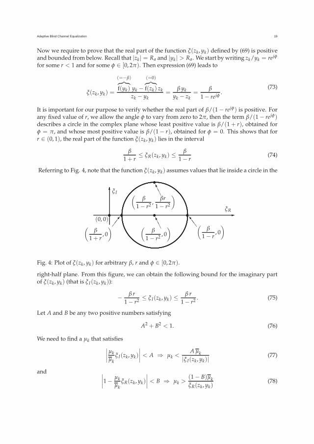
Referring to Fig. 4, note that the function ξ(zk, yk) assumes values that lie inside a circle in the

-

6

(0, 0)s s s

s

s

ξ I

ξR

(β

1 + r, 0

)��7 (

β

1 − r, 0

)SSo(β

1 − r2, 0

)AAK

(β

1 − r2,

βr

1 − r2

)AAK

Fig. 4: Plot of ξ(zk, yk) for arbitrary β, r and φ ∈ [0, 2π).

right-half plane. From this figure, we can obtain the following bound for the imaginary partof ξ(zk, yk) (that is ξ I(zk, yk)):

− β r

1 − r2≤ ξ I(zk, yk) ≤

β r

1 − r2. (75)

Let A and B be any two positive numbers satisfying

A2 + B2< 1. (76)

We need to find a µk that satisfies

∣∣∣∣µk

µk

ξ I(zk, yk)

∣∣∣∣ < A ⇒ µk <A µk

|ξ I(zk, yk)|(77)

and ∣∣∣∣1 −µk

µk

ξR(zk, yk)

∣∣∣∣ < B ⇒ µk >(1 − B)µk

ξR(zk, yk)(78)


Combining (77) and (78), we obtain

0 <(1 − B)µk

ξR(zk, yk)< µk <

A µk

|ξ I(zk, yk)|< 1 (79)

Using the extremum values of ξR(zk, yk) and ξ I(zk, yk), we obtain

(1 + r)(1 − B)

β ‖xk‖2< µk <

(1 − r2)A

β r‖xk‖2(80)

We need to guarantee that the upper bound in the above expression is larger than the lowerbound. This can be achieved by choosing {A, B} properly such that

0 < (1 − B) <1 − r

rA < 1 (81)

From our initial assumptions that the equalizer is in the vicinity of open-eye solution and|yk| > Ra, we know that r < 1. It implies that we require to determine the smallest value of rwhich satisfies (81), or in other words, we have to determine the bound for step-size with thelargest equalizer output amplitude. In Fig. 5(a), we plot the function fr := (1 − r)/r versus r;note that for 0.5 ≤ r < 1 we have fr ≤ 1.

1/5 1/2 1 0

1

4

r

f r = (

1−

r)/r

0 0.2 0.4 0.6 0.8 1−0.5

−0.4

−0.3

−0.2

−0.1

0

B

f B

ρ = 1

ρ = 0.8

ρ = 0.6

ρ = 0.4

ρ = 0.2

a) b)

Fig. 5: Plots: a) fr and b) fB.

Let {Ao, Bo} be such that (1 − Bo) = ρAo, where 0 < ρ < 1. To satisfy (81), we need 0.5 ≤ r <1 and ρ < (1 − r)/r. From (76), Bo must be such that

(1 − Bo)2 ρ−2 + B2

o < 1 (82)

which reduces to the following quadratic inequality in Bo:

(1 + ρ−2

)B2

o − 2ρ−2Bo +(

ρ−2 − 1)< 0. (83)

If we find a Bo that satisfies this inequality, then a pair {Ao, Bo} satisfying (76) and (81) exists.So consider the quadratic function fB :=

(1 + ρ−2

)B2 − 2ρ−2B +

(ρ−2 − 1

). It has a negative

minimum and it crosses the real axis at the positive roots B(1) =(1 − ρ2

)/(1 + ρ2

), and


B(2) = 1. This means that there exist many values of B, between the roots, at which thequadratic function in B evaluates to negative values (refer to Fig. 5(b)).

Hence, Bo falls in the interval (1 − ρ2)/(1 + ρ2) < Bo < 1; it further gives Ao = 2ρ/(1 + ρ2

).

Using {Ao, Bo}, we obtain

3ρ2

β (1 + ρ2) ‖xk‖2< µk <

3ρ

β (1 + ρ2) ‖xk‖2(84)

Note that, arg minρ ρ2/(1 + ρ2) = 0, and arg maxρ ρ/(1 + ρ2) = 1. So making ρ = 0 and ρ = 1

in the lower and upper bounds, respectively, and replacing ‖xk‖2 with E[‖xk‖2

], we find the

widest stochastic stability bound on µk as follows:

0 < µ <3

2βE [‖xk‖2]. (85)

The significance of (85) is that it can easily be measured from the equalizer input samples. Inadaptive filter theory, it is convenient to replace E

[‖xk‖2

]with tr (R), where R = E

[xkxH

k

]

is the autocorrelation matrix of channel observation. Also note that, when noise is negligibleand channel coefficients are normalized, the quantity tr (R) can be expressed as the productof equalizer length (N) and transmitted signal average energy (Pa); it gives

0 < µβCMA <3

2βNPa(86)

Note that the bound (86) is remarkably similar to the stability bound of complex-valued LMSalgorithm (refer to expression (20)). Comparing (86) and (20), we obtain a simple and elegantrelation between the step-sizes of βCMA and complex-valued LMS:

µβCMA

µLMS<

3

β. (87)

6. Simulation results

We compare βCMA with CMA (Equation (27)) and SFA (Equation (40)). We considertransmission of amplitude-phase shift-keying (APSK) signals over a complex voice-bandchannel (channel-1), taken from Picchi & Prati (1987), and evaluate the average ISI tracesat SNR = 30dB. We employ a seven-tap equalizer with central spike initialization and use8- and 16-APSK signalling. Step-sizes have been selected such that all algorithms reachedsteady-state requiring same number of iterations. The parameter β is obtained as:

β =

{1.535, for 8.APSK1.559, for 16.APSK

(88)

Results are summarized in Fig. 6; note that the βCMA performed better than CMA and SFAby yielding much lower ISI floor. Also note that SFA performed slightly better than CMA.

Next we validate the stability bound (86). Here we consider a second complex channel (aschannel-2) taken from Kennedy & Ding (1992). In all cases, the simulations were performedwith Nit = 104 iterations, Nrun = 100 runs, and no noise. In Fig. 7, we plot the probability


0 500 1000 1500 2000 2500 3000 3500 4000−28

−24

−20

−16

−12

−8

Iterations

Residual ISI [dB] traces 8.APSK: SNR = 30dB

CMA: µ = 8E−4 SFA: µ = 7E−4 βCMA: µ = 6E−4, β = 1.53

−2 0 2−2

0

2Test signal SFACMA

βCMA

0 500 1000 1500 2000 2500 3000 3500 4000−28

−24

−20

−16

−12

−8

Iterations

Residual ISI [dB] traces 16.APSK: SNR = 30dB CMA: µ = 1.5E−4 SFA: µ = 1.3E−4

βCMA: µ = 3E−4, β = 1.55

−3 0 3−3

0

3Test signal

βCMA

CMA SFA

a) b)

Fig. 6: Residual ISI: a) 8-APSK and b) 16-APSK. The inner and outer moduli of 8-APSK are1.000 and 1.932, respectively. And the inner and outer moduli of 16-APSK are 1.586 and 3.000,respectively. The energies of 8-APSK and 16-APSK are 2.366 and 5.757, respectively.

1 1.1 1.2 1.3 1.4 1.50

0.2

0.4

0.6

0.8

1

µ_norm

P_d

iv

8APSK

N = 7

N = 17

N = 27

Channel 2 [KD]Channel 1 [PP]

1 1.1 1.2 1.3 1.4 1.50

0.2

0.4

0.6

0.8

1

µ_norm

P_d

iv

16APSK

N = 7

N = 17

N = 27

Channel 2 [KD]Channel 1 [PP]

a) b)

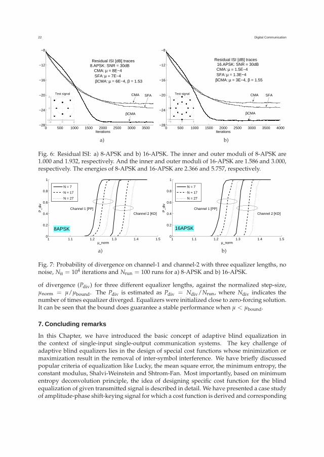
Fig. 7: Probability of divergence on channel-1 and channel-2 with three equalizer lengths, nonoise, Nit = 104 iterations and Nrun = 100 runs for a) 8-APSK and b) 16-APSK.

of divergence (Pdiv) for three different equalizer lengths, against the normalized step-size,µnorm = µ/µbound. The Pdiv is estimated as Pdiv = Ndiv/Nrun, where Ndiv indicates thenumber of times equalizer diverged. Equalizers were initialized close to zero-forcing solution.It can be seen that the bound does guarantee a stable performance when µ < µbound.

7. Concluding remarks

In this Chapter, we have introduced the basic concept of adaptive blind equalization inthe context of single-input single-output communication systems. The key challenge ofadaptive blind equalizers lies in the design of special cost functions whose minimization ormaximization result in the removal of inter-symbol interference. We have briefly discussedpopular criteria of equalization like Lucky, the mean square error, the minimum entropy, theconstant modulus, Shalvi-Weinstein and Shtrom-Fan. Most importantly, based on minimumentropy deconvolution principle, the idea of designing specific cost function for the blindequalization of given transmitted signal is described in detail. We have presented a case studyof amplitude-phase shift-keying signal for which a cost function is derived and corresponding


adaptive algorithm is obtained. We have also addressed the admissibility of the proposedcost function and stability of the corresponding algorithm. The blind adaptation of thederived algorithm is shown to possess better convergence behavior compared to two existingalgorithms. Finally, hints are provided to obtain blind equalization cost functions for squareand cross quadrature amplitude modulation signals.

8. Exercises

1. Refer to Fig. 8 for geometrical details of square- and cross-QAM signals. Now following theideas presented in Section 5, show that the blind equalization cost functions for square- andcross-QAM signals are respectively as follows:

maxw

E

[|yn|2

], s.t. max {|yR,n| , |yI,n|} ≤ R. (89)

and

maxw

E

[|yn|2

], s.t. max {|ρ yR,n| , |yI,n|}+ max {|yR,n| , |ρ yI,n|} − max {|yR,n| , |yI,n|} ≤ ρR.

(90)

R

RX

Y

R

RX

Y

ρR

(1−ρ)R

a) b)

Fig. 8: Geometry of a) square- and b) cross-QAM(

ρ = 23

).

2. By exploiting the independence between the in-phase and quadrature components ofsquare QAM signal, show that the following blind equalization cost function may be obtained:

maxw

E

[|yn|2

], s.t. max {|yR,n|} = max {|yI,n|} ≤ R. (91)

The cost (91) originally appeared in Satorius & Mulligan (1993). Refer to Meng et al. (2009)and Abrar & Nandi (2010a), respectively, for its block-iterative and adaptive optimization.

9. Acknowledgment

The authors acknowledge the support of COMSATS Institute of Information Technology,Islamabad, Pakistan, King Fahd University of Petroleum and Minerals, Dhahran, SaudiArabia, and the University of Liverpool, UK towards the accomplishment of this work.


10. References

Abrar, S. & Nandi, A.K. (2010a). Adaptive solution for blind equalization and carrier-phaserecovery of square-QAM, IEEE Sig. Processing Lett. 17(9): 791–794.

Abrar, S. & Nandi, A.K. (2010b). Adaptive minimum entropy equalization algorithm, IEEECommun. Lett. 14(10): 966–968.

Abrar, S. & Nandi, A.K. (2010c). An adaptive constant modulus blind equalization algorithmand its stochastic stability analysis, IEEE Sig. Processing Lett. 17(1): 55–58.

Abrar, S. & Nandi, A.K. (2010d). A blind equalization of square-QAM signals: a multimodulusapproach, IEEE Trans. Commun. 58(6): 1674–1685.

Abrar, S. & Shah, S. (2006a). New multimodulus blind equalization algorithm with relaxation,IEEE Sig. Processing Lett. 13(7): 425–428.

Abrar, S. & Qureshi, I.M. (2006b). Blind equalization of cross-QAM signals, IEEE Sig.Processing Lett. 13(12): 745–748.

Abrar, S., Zerguine, A. & Deriche, M. (2005). Soft constraint satisfaction multimodulus blindequalization algorithms, IEEE Sig. Processing Lett. 12(9): 637–640.

Allen, J. & Mazo, J. (1973). Comparison of some cost functions for automatic equalization,IEEE Trans. Commun. 21(3): 233–237.

Allen, J. & Mazo, J. (1974). A decision-free equalization scheme for minimum-phase channels,IEEE Trans. Commun. 22(10): 1732–1733.

Baykal, B., Tanrikulu, O., Constantinides, A. & Chambers, J. (1999). A new family of blindadaptive equalization algorithms, IEEE Sig. Processing Lett. 3(4): 109–110.

Bellini, S. (1986). Bussgang techniques for blind equalization, Proc. IEEE GLOBECOM’86pp. 1634–1640.

Bellini, S. (1994). Bussgang techniques for blind deconvolution and equalization, in Blinddeconvolution, S. Haykin (Ed.), Prentice Hall, pp. 8–59.

Benedetto, F., Giunta, G. & Vandendorpe, L. (2008). A blind equalization algorithm based onminimization of normalized variance for DS/CDMA communications, IEEE Trans.Veh. Tech. 57(6): 3453–3461.

Benveniste, A. & Goursat, M. (1984). Blind equalizers, IEEE Trans. Commun. 32(8): 871–883.Benveniste, A., Goursat, M. & Ruget, G. (1980a). Analysis of stochastic approximation

schemes with discontinous and dependent forcing terms with applications to datacommunications algorithms, IEEE Trans. Automat. Contr. 25(12): 1042–1058.

Benveniste, A., Goursat, M. & Ruget, G. (1980b). Robust identification of a nonminimumphase system: Blind adjustment of a linear equalizer in data communication, IEEETrans. Automat. Contr. 25(3): 385–399.

Claerbout, J. (1977). Parsimonious deconvolution, SEP-13 .C.R. Johnson, Jr., Schniter, P., Endres, T., Behm, J., Brown, D. & Casas, R. (1998).

Blind equalization using the constant modulus criterion: A review, Proc. IEEE86(10): 1927–1950.

Ding, Z. & Li, Y. (2001). Blind Equalization and Identification, Marcel Dekker Inc., New York.Donoho, D. (1980). On minimum entropy deconvolution, Proc. 2nd Applied Time Series Symp.

pp. 565–608.Farhang-Boroujeny, B. (1998). Adaptive Filters, John Wiley & Sons.Fiori, S. (2001). A contribution to (neuromorphic) blind deconvolution by flexible

approximated Bayesian estimation, Signal Processing 81: 2131–2153.


Garth, L., Yang, J. & Werner, J.-J. (1998). An introduction to blind equalization, ETSI/STSTechnical Committee TM6, Madrid, Spain pp. TD7: 1–16.

Godard, D. (1980). Self-recovering equalization and carrier tracking in two-dimensional datacommunications systems, IEEE Trans. Commun. 28(11): 1867–1875.

Goupil, A. & Palicot, J. (2007). New algorithms for blind equalization: the constant normalgorithm family, IEEE Trans. Sig. Processing 55(4): 1436–1444.

Gray, W. (1978). Variable norm deconvolution, SEP-14 .Gray, W. (1979a). A theory for variable norm deconvolution, SEP-15 .Gray, W. (1979b). Variable Norm Deconvolution, PhD thesis, Stanford Univ.Haykin, S. (1994). Blind deconvolution, Prentice Hall.Haykin, S. (1996). Adaptive Filtering Theory, Prentice-Hall.Im, G.-H., Park, C.-J. & Won, H.-C. (2001). A blind equalization with the sign algorithm for

broadband access, IEEE Commun. Lett. 5(2): 70–72.Kennedy, R. & Ding, Z. (1992). Blind adaptive equalizers for quadrature amplitude modulated

communication systems based on convex cost functions, Opt. Eng. 31(6): 1189–1199.Lucky, R. (1965). Automatic equalization for digital communication, The Bell Systems Technical

Journal XLIV(4): 547–588.Lucky, R. (1966). Techniques for adaptive equalization of digital communication systems, The

Bell Systems Technical Journal pp. 255–286.Meng, C., Tuqan, J. & Ding, Z. (2009). A quadratic programming approach to blind

equalization and signal separation, IEEE Trans. Sig. Processing 57(6): 2232–2244.Nikias, C. & Petropulu, A. (1993). Higher-order spectra analysis a nonlinear signal processing

framework, Englewood Cliffs, NJ: Prentice-Hall.Ooe, M. & Ulrych, T. (1979). Minimum entropy deconvolution with an exponential

transformation, Geophysical Prospecting 27: 458–473.Picchi, G. & Prati, G. (1987). Blind equalization and carrier recovery using a ‘stop-and-go’

decision-directed algorithm, IEEE Trans. Commun. 35(9): 877–887.Pinchas, M. & Bobrovsky, B.Z. (2006). A maximum entropy approach for blind deconvolution,

Sig. Processing 86(10): 2913–2931.Pinchas, M. & Bobrovsky, B.Z. (2007). A novel HOS approach for blind channel equalization,

IEEE Trans. Wireless Commun. 6(3): 875–886.Romano, J., Attux, R., Cavalcante, C. & Suyama, R. (2011). Unsupervised Signal Processing:

Channel Equalization and Source Separation, CRC Press Inc.Rupp, M. & Sayed, A.H. (2000). On the convergence analysis of blind adaptive equalizers for

constant modulus signals, IEEE Trans. Commun. 48(5): 795–803.Sato, Y. (1975). A method of self-recovering equalization for multilevel amplitude modulation

systems, IEEE Trans. Commun. 23(6): 679–682.Satorius, E. & Mulligan, J. (1992). Minimum entropy deconvolution and blind equalisation,

IEE Electronics Lett. 28(16): 1534–1535.Satorius, E. & Mulligan, J. (1993). An alternative methodology for blind equalization, Dig. Sig.

Process.: A Review Jnl. 3(3): 199–209.Serra, J. & Esteves, N. (1984). A blind equalization algorithm without decision, Proc. IEEE

ICASSP 9(1): 475–478.Shalvi, O. & Weinstein, E. (1990). New criteria for blind equalization of non-minimum phase

systems, IEEE Trans. Inf. Theory 36(2): 312–321.Shtrom, V. & Fan, H. (1998). New class of zero-forcing cost functions in blind equalization,

IEEE Trans. Signal Processing 46(10): 2674.


Sidak, Z., Sen, P. & Hajek, J. (1999). Theory of Rank Tests, Academic Press; 2/e.Treichler, J. & Agee, B. (1983). A new approach to multipath correction of constant modulus

signals, IEEE Trans. Acoust. Speech Signal Processing 31(2): 459–471.Treichler, J. R. & Larimore, M. G. (1985). New processing techniques based on the

constant modulus adaptive algorithm, IEEE Trans. Acoust., Speech, Sig. Process.ASSP-33(2): 420–431.

Tugnait, J.K., Shalvi, O. & Weinstein, E. (1992). Comments on ‘New criteria for blinddeconvolution of nonminimum phase systems (channels)’ [and reply], IEEE Trans.Inf. Theory 38(1): 210–213.

Walden, A. (1985). Non-Gaussian reflectivity, entropy, and deconvolution, Geophysics50(12): 2862–2888.

Walden, A. (1988). A comparison of stochastic gradient and minimum entropy deconvolutionalgorithms, Signal Processing 15: 203–211.

Wesolowski, K. (1987). Self-recovering adaptive equalization algorithms for digital radio andvoiceband data modems, Proc. European Conf. Circuit Theory and Design pp. 19–24.

Widrow, B. & Hoff, M.E. (1960). Adaptive switching circuits, Proc. IRE WESCON Conf. Rec.pp. 96–104.

Widrow, B., McCool, J. & Ball, M. (1975). The complex LMS algorithm, Proc. IEEE63(4): 719–720.

Wiggins, R. (1977). Minimum entropy deconvolution, Proc. Int. Symp. Computer Aided SeismicAnalysis and Discrimination .

Wiggins, R. (1978). Minimum entropy deconvolution, Geoexploration 16: 21–35.Yang, J., Werner, J.-J. & Dumont, G. (2002). The multimodulus blind equalization and its

generalized algorithms, IEEE Jr. Sel. Areas Commun. 20(5): 997–1015.Yuan, J.-T. & Lin, T.-C. (2010). Equalization and carrier phase recovery of CMA and MMA in

blind adaptive receivers, IEEE Trans. Sig. Processing 58(6): 3206–3217.Yuan, J.-T. & Tsai, K.-D. (2005). Analysis of the multimodulus blind equalization algorithm in

QAM communication systems, IEEE Trans. Commun. 53(9): 1427–1431.

Adaptive Blind Channel Equalizationww3.comsats.edu.pk/faculty/users/ee/sabrar/abrar_third.pdf ·...

Documents

Transcript of Adaptive Blind Channel Equalizationww3.comsats.edu.pk/faculty/users/ee/sabrar/abrar_third.pdf ·...