ADAPTIVE BEAMFORMING APPROACHES FOR SMART …docs.neu.edu.tr/library/6501550494.pdfADAPTIVE...
85
ADAPTIVE BEAMFORMING APPROACHES FOR SMART ANTENNA SYSTEMS A THESIS SUBMITTED TO THE GRADUATE SCHOOL OF APPLIED SCIENCES OF NEAR EAST UNIVERSITY By RAWAN MANSOUR In Partial Fulfillment of the Requirements for The Degree of Master of Science in Electrical and Electronic Engineering NICOSIA, 2016 RAWAN MANSOUR ADAPTIVE BEAMFORMING APPROACHES FOR SMART ANTENNA SYSTEMS NEU 2016
Transcript of ADAPTIVE BEAMFORMING APPROACHES FOR SMART …docs.neu.edu.tr/library/6501550494.pdfADAPTIVE...
ADAPTIVE BEAMFORMING APPROACHES FOR
SMART ANTENNA SYSTEMS
A THESIS SUBMITTED TO THE GRADUATE
SCHOOL OF APPLIED SCIENCES
OF
NEAR EAST UNIVERSITY
By
RAWAN MANSOUR
In Partial Fulfillment of the Requirements for
The Degree of Master of Science
in
Electrical and Electronic
Engineering
NICOSIA, 2016
RA
WA
N M
AN
SO
UR
A
DA
PT
IVE
BE
AM
FO
RM
ING
AP
PR
OA
CH
ES
FO
R
SM
AR
T A
NT
EN
NA
SY
ST
EM
S
NE
U
2016

ADAPTIVE BEAMFORMING APPROCHES FOR
SMART ANTENNA SYSTEMS
A THESIS SUBMITTED TO THE GRADUATE
SCHOOL OF APPLIED SCIENCES
OF
NEAR EAST UNIVERSITY
By
RAWAN MANSOUR
In Partial Fulfillment of the Requirements for
The Degree of Master of Science
in
Electrical and Electronic
Engineering
NICOSIA, 2016
Rawan MANSOUR: ADAPTIVE BEAMFORMING APPROACHES FOR
SMART ANTENNA SYSTEMS
Approval of Director of Graduate School of
Applied Sciences
Prof. Dr. İlkay SALİHOĞLU
We certify this thesis is satisfactory for the award of the degree of Masters of
Science in Electrical and Electronic Engineering
Examining Committee in Charge:

i
I hereby declare that all information in this document has been obtained and presented in
accordance with academic rules and ethical conduct. I also declare that, as required by
these rules and conduct, I have fully cited and referenced all material and results that are
not original to this work.
Name, Last name: Rawan Mansour
Signature:
Date:

ii
ACKNOWLEDGMENTS
I would like to express my sincere appreciation and thanks to my supervisor, Dr. Refet
Ramiz, for his guidance and support throughout my study and thesis preparation. His
knowledge, advices and creative thinking were the source of inspiration throughout this
work.
I would also like to express my gratitude to my mother, my father, brothers, and sisters
for their support, patience, and feelings of love all over my life. Your constant love was
the source of motivation for me to go on my way. The prayers of my mother and
support of my father filled me with sense of pleasure and strengthened me always.
I would like to thank my beloved father Mohammed Mansour for his encouragements and
continuous love. A special thank to my dearest brother Bassil Mansour with whom I
passed most of my time abroad and who helped me always to reach my goals.
Last but never the least, I am thankful to my friends and colleagues in Near East
University and abroad for their unlimited support, thank you all.

iii
To my lovely family….
iv
ABSTRACT
Smart antenna is considered as promising technology in wireless communication systems.
It provides powerful solutions in the area of wireless networks. This system is capable of
increasing the capacity, coverage, enhancing the control power and service quality, as well
as reducing the co-channel interference and effects of multipath fading. Adaptive beam-
forming is one of the main and most famous aspects in the development of smart antenna
technologies. It uses different topologies and algorithms to identify the desired signals and
separate the interference from a channel. Algorithms like Recursive Least Square (RLS),
Constant Modulus Algorithm (CMA), and Least Mean Square algorithm (LMS) has proved
their efficiency in adaptive beam-forming techniques. However, the increasing
requirements in communication systems imply more focus on the implementation of the
artificial intelligence in smart antennas.
Neural networks have witnessed fast development in the last three decades, ANNs has the
ability to increase the efficiency and optimize the use of smart antennas in wireless
communication systems. This work is sacrificed for the study and discussion of the smart
antenna technology and the adaptive beam-forming approaches. It also provides an
introduction to the implementation of back propagation neural networks in smart antenna
as an adaptive beam-forming technique. Comparison and performance evaluation of these
algorithms in terms of complexity, stability, convergence speed, amplitude response and
tracking of desired signal will be present. The algorithms will be implemented in the
MATLAB environment and results will be presented and discussed.
Keywords: Smart antenna; adaptive antenna array; beam-forming algorithms; LMS; neural
networks.

v
ÖZET

vi
TABLE OF CONTENTS
ACKNOWLEDGMENTS .................................................................................................. II
ABSTRACT ....................................................................................................................... IV
ÖZET ................................................................................................................................... V
TABLE OF CONTENTS .................................................................................................. VI
LIST OF FIGURES ........................................................................................................... IX
LIST OF TABLES ............................................................................................................. XI
LIST OF ABBREVIATIONS ......................................................................................... XII
CHAPTER 1 ......................................................................................................................... 1
INTRODUCTION ............................................................................................................... 1
1.1 INTRODUCTION ............................................................................................................. 1
1.2 LITERATURE REVIEW .................................................................................................... 2
CHAPTER 2 ......................................................................................................................... 4
ANTENNA AND ANTENNAS SYSTEMS ....................................................................... 4
2.1 ANTENNA ..................................................................................................................... 4
2.2 ANTENNA PARAMETERS ............................................................................................... 5
2.2.1 Radiation pattern .................................................................................................. 5
2.2.2 Antenna gain ......................................................................................................... 6
2.2.3 Bandwidth ............................................................................................................. 6
2.2.4 Polarization ........................................................................................................... 6
2.3 ANTENNA CLASSIFICATION .......................................................................................... 7
2.3.1 Isotropic antenna................................................................................................... 7
2.3.2 Omni directional antennas .................................................................................... 7
2.3.3 Directional Antennas ............................................................................................ 8
2.3.4 Antenna array ....................................................................................................... 9
2.3.4.1 Phased array ....................................................................................................... 9
2.3.4.2 Adaptive array ................................................................................................... 9
2.3.4.3 Smart antenna .................................................................................................. 10

vii
2.4 ANTENNA SYSTEMS AND THE QUEST FOR MORE CAPACITY IN CELLULAR RADIO
SYSTEM ............................................................................................................................ 10
CHAPTER 3 ....................................................................................................................... 12
3.1 SMART ANTENNA SYSTEM CONCEPT .......................................................................... 13
3.1.1 Analogy for adaptive smart antenna ................................................................... 13
3.2 TYPES OF SMART ANTENNA SYSTEMS ........................................................................ 14
3.2.1 Switched-beam systems ...................................................................................... 14
3.2.2 Adaptive-array systems ...................................................................................... 15
3.3 ARCHITECTURE OF SMART ANTENNA SYSTEM ........................................................... 16
3.3.1 Antenna array ..................................................................................................... 16
3.3.1.1 Antenna array geometry .................................................................................. 17
3.3.1.2 Theoretical model for an antenna array ........................................................... 18
3.3.2 Radio unit (hardware) ......................................................................................... 19
3.3.3 Signal processing unit ......................................................................................... 20
3.3.3.1 DOA estimator ................................................................................................. 20
3.3.3.2 Adaptive beamformer ...................................................................................... 21
3.4 THE GOAL OF SMART ANTENNA .................................................................................. 22
3.5 THE DRAWBACKS ........................................................................................................ 23
CHAPTER 4 ....................................................................................................................... 25
1.4 FIXED WEIGHT BEAM-FORMING BASICS ..................................................................... 25
4.1.1 Maximum signal-to-interference ratio approach ................................................ 25
4.1.2 Minimum mean-square error approach .............................................................. 28
4.1.3 Maximum likelihood approach ........................................................................... 29
4.1.4 Minimum Variance approach ............................................................................. 30
4.2 ADAPTIVE BEAM FORMING ......................................................................................... 31
4.2.1 Least mean square algorithm (LMS) .................................................................. 31
4.2.2 Recursive least square algorithm (RLS) ............................................................. 32
4.2.3 Constant-modulus (CM) algorithm .................................................................... 33
CHAPTER 5 ....................................................................................................................... 35
5.1 OVERVIEW OF THE CHAPTER ...................................................................................... 36
5.2 HUMAN BRAIN VS. ARTIFICIAL NEURAL NETWORKS .................................................. 36
viii
5.3 ARTIFICIAL NEURAL NETWORKS ................................................................................ 38
5.4 BASIC ELEMENTS OF ARTIFICIAL NETWORK ............................................................... 39
5.4.1 ANN layers ......................................................................................................... 39
5.4.2 Weights in ANNs ............................................................................................... 40
5.4.3 Transfer functions ............................................................................................... 41
5.4.3.1 Linear activation functions .............................................................................. 41
5.4.3.2 Threshold limit transfer function ..................................................................... 42
5.4.3.3 Sigmoid transfer function ................................................................................ 42
5.5 LEARNING OF THE ARTIFICIAL NEURAL NETWORKS ................................................... 43
5.5.1 Feed forward back propagation training algorithm ............................................ 43
5.6 BACK PROPAGATION ALGORITHM’S MODEL .............................................................. 45
CHAPTER 6 ....................................................................................................................... 47
6.1 COMPARISON OF AMPLITUDE RESPONSES OF LMS, RLS AND CMA ALGORITHMS .... 47
6.1.1 LMS algorithm ................................................................................................... 47
6.1.2 RLS algorithm .................................................................................................... 48
6.1.3 CMA algorithm .................................................................................................. 49
6.2 THE TRACKING PERFORMANCE OF ADAPTIVE BEAM-FORMING ALGORITHM ............. 51
6.3 SCOPE ON THE RESULTS .............................................................................................. 54
6.4 NEURAL NETWORKS FOR SMART ANTENNA OPTIMIZATION ....................................... 55
6.5 EFFECT OF N AND D ON THE AMPLITUDE FACTOR ...................................................... 57
6.6 ANN PERFORMANCE IN ACQUISITION AND TRACKING OF DESIRED SIGNAL .............. 58
6.7 ARRAY FACTOR WITH VARIATION OF NETWORK PARAMETERS .................................. 59
6.8 EVALUATION OF ADAPTIVE BEAM FORMING METHODS.............................................. 61
CONCLUSIONS ................................................................................................................ 64
ix
LIST OF FIGURES
Figure 2.1: Two dimensional field pattern plot ..............................................................
Figure 2.2: Coverage pattern for omni-directional antenna ..........................................
Figure 2.3: Converge pattern for Sectorized antenna system .......................................................
Figure 2.4: a) Adaptive antenna array. b) Phased antenna array ..................................
Figure 3.1: Smart antenna analogy .................................................................................
Figure 3.2: Switched-beam coverage pattern .................................................................
Figure 3.3: Adaptive array coverage ..............................................................................
Figure 3.4: Different types of uniform array geometries. ..............................................
Figure 3.5: ULA with N sensors ....................................................................................
Figure 3.6: The hardware part in smart antenna (receiving section) ..............................
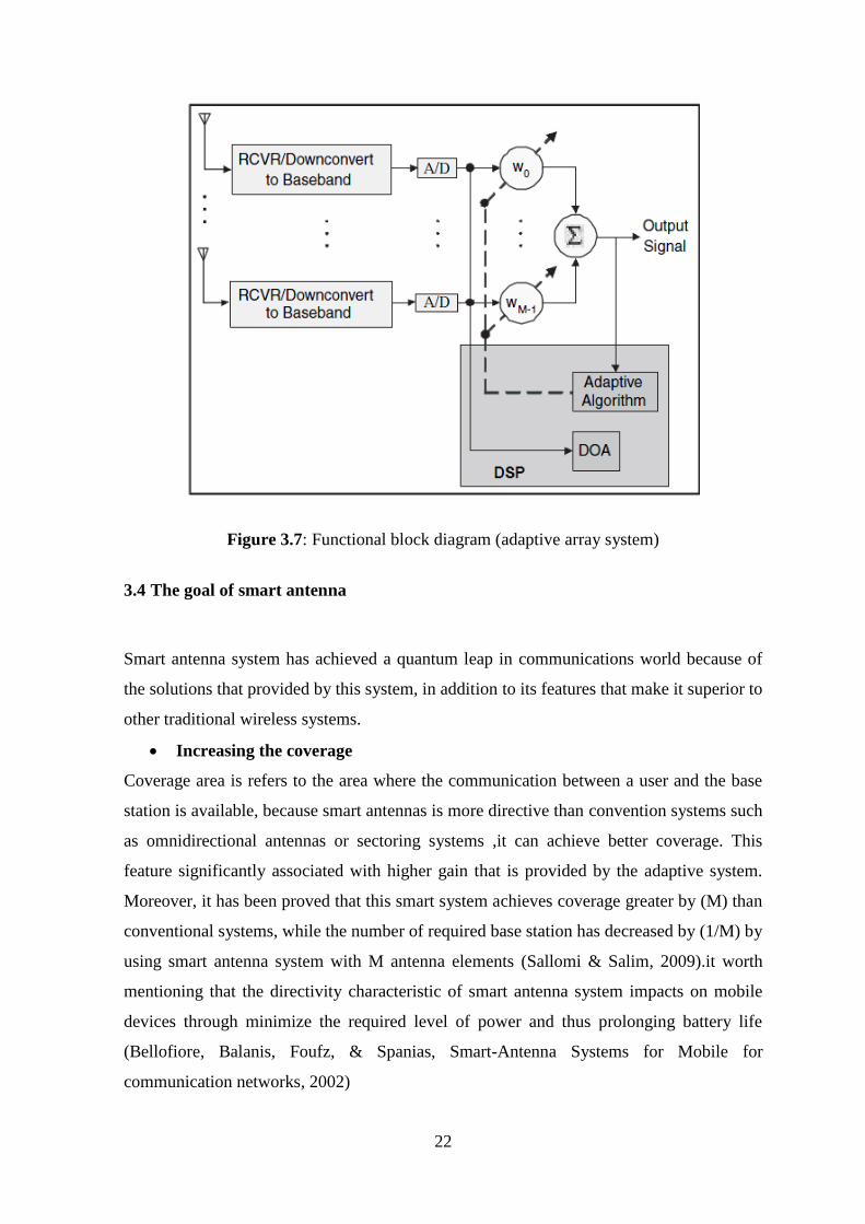
Figure 3.7: Functional block diagram (adaptive array system) ......................................
Figure 4.1: M-element array with desired signal and N interfering signals ...................
Figure 4.2: Block diagram for MSE adaptive system ....................................................
Figure 1.1: Connections between biological neurons ....................................................
Figure 1.2: Elements of biological neuron .....................................................................
Figure 1.3: Analogy between human brain and neural networks ...................................
Figure 1.4: Construction of artificial neural network ....................................................
Figure 1.5: Layer concept in artificial neural networks .................................................
Figure 1.6: Linear ramped transfer function ..................................................................
Figure 1.7: Threshold transfer function..........................................................................
Figure 1.8: Logarithmic and tangential sigmoid transfer functions ..............................
Figure 1.9: Structure of network and error propagation ................................................
Figure 6.1: Array Factor plots for LMS algorithm (d=0.5λ) .........................................
Figure 6.2: Array Factor plots for LMS algorithm ........................................................
Figure 6.3: Amplitude response by using RLS algorithm with d=0.5λ .........................
Figure 6.4: Amplitude response by using RLS algorithm with d=0.25λ.......................
Figure 6.5: Amplitude response by using RLS algorithm with d=0.125λ .....................
Figure 6.6: Amplitude response by using CMA algorithm with d=0.5λ .......................
Figure 6.7: Amplitude response by using CMA algorithm with d=0. 25λ ....................
Figure 6.8: Amplitude response by using CMA algorithm with d=0.125λ ...................
Figure 6.9: Acquisition and tracking of desired signal for LMS algorithm ...................
Figure 6.10: mean square error in LMS algorithm(N=8,d=0.5).....................................
x
Figure 6.11: Magnitude of array weights in LMS algorithm .........................................
Figure 6.12: Magnitude of array weights in RLS algorithm ..........................................
Figure 6.13: Mean Square Error in RLS algorithm ........................................................
Figure 6.14: Acquisition and tracking of desired signal for RLS algorithm ..................
Figure 6.15: Neural network diagram ............................................................................
Figure 6.16: Back-propagation learning .........................................................................
Figure 6.17: Amplitude response by using ANN with d=0. 5λ and different N ............
Figure 6.18: Amplitude response by using ANN with d=0. 25λ and different N ..........
Figure 6.19: Amplitude response by using ANN with d=0. 125λ and different N ........
Figure 6.20: Acquisition and tracking of desired signal for ANN .................................
Figure 6.21: Mean Square Error in ANN method ..........................................................
Figure 6.22: Amplitude response for the first expirment by using ANN with two
hidden layers(4,5) respectively ..................................................................
Figure 6.23: Acquisition and tracking of desired signal for LMS,RLS and ANN .........
Figure 6.24: Amplitude response for the second expirment by using ANN with one
hidden layers of size=10 ............................................................................

xi
LIST OF TABLES
Table 6.1: Parameters of the desired and interference AOA ........................................
Table 6.2: Final parameters of the used neural networks .............................................
Table 6.3: Parameters of the used ANN .......................................................................
xii
LIST OF ABBREVIATIONS
AF: Amplitude factor
ANN: Artificial neural networks
AOA: Angle of arrival
DOA: Direction of arrival
LMS: Least mean square
CMA: Constant modulus algorithm
RLS: Recursive least square
E: Expectation
SAS: Smart antenna system
ULA: uniform linear array

xiii
1
CHAPTER 1
INTRODUCTION
1.1 Introduction
In the field of communications, antenna is an electrical device which converts electric
waves into electromagnetic waves or convert electromagnetic waves into electric waves.
The dramatic growth of wireless communication industry has resulted in searches for new
technologies to overcome some problems associated with multipath such as fading, phase
cancellation and delay spread in addition to problems associated with co-channel
interferences.
Smart antennas are of the most important elements introduced into wireless
communication systems nowadays. This is due to its special features and characteristics.
However, The future implementation of techniques of smart antenna in wireless structures
is likely to affect considerably the efficiency of spectrum employment, to minimize the
price of new networks establishment, ameliorate the quality of service, and to simplify the
inter-operation across different wireless network technologies. SAS are also able to
eliminate or reduce the troubles caused by multi path propagation of waves. Recently,
smart antennas have became very popular in different areas such as Cellular systems,
wireless networks, radar systems, and electronic warfare (EWF) as a counter measure to
electronic jamming and satellite systems.
The most important characteristics of smart antenna systems reside in their ability to
maximize the gain of the antenna in the desired direction and attenuate the gain in
interference directions. Therefore, smart antennas are able to reduce noise and interference
that affect the desired signals, and thus increase the efficiency and performance of the
wireless system. Smart antennas are using developed processing algorithms to ensure
higher signal to noise ration upon reception of data, and due to the revolution in the use of
communication systems, the need for more efficient, developed, and easy to implement
algorithms is continuously increasing.
Artificial neural networks are very efficient and strong tools that have become popular in
the recent decades. They are widely implemented in different scientific fields from control
systems, power engineering, communication, financial sciences, banking, weather
prediction and many other fields. ANNs have proved their extensive capability to offer
2
high performance in solving different non linear problems that can’t be solved easily by
using traditional means.
This work will introduce the application of artificial neural networks in the function of
smart antenna systems. The artificial neural networks will be implemented to optimize the
performance of the system. Comparison between the most popular adaptive beamforming
algorithms and ANNs algorithm for smart antenna will be carried out. Back propagation
ANN algorithm will be implemented using MATLAB and its function to determine the
weights of the antenna elements in order to minimize the errors in the received signal.
Simulation result will be discussed and presented upon the end of this work.
1.2 Literature Review
The use of smart antenna is indispensable for the modern wireless communication systems.
Researchers have started focusing on the smart antenna decades ago. Since then, different
ideas, techniques, algorithms, and designs have been proposed and studied in literature.
Smart antenna systems are developing and new ideas are being created with the sunrise of
every new day. Zooghby, Christodoulou, & Georgiopoulos, (2000) has considered the
problem of multiple source tracking using smart antenna relied on neural networks. The
proposed system was implemented for terrestrial and satellite mobile communication
systems. Radial basis function neural networks RBFNN algorithm was used to build a
neural multiple sources tracking system. The neural network algorithm was used to
perform detection and direction of arrival. The main advantage of this algorithm is that it
needs no prior knowledge of the number of sources of signal; over more, it offers high
accuracy and can locate sources that are greater than the number of elements of the
antenna. The use of auto regressive (ARNN) and adaptive linear neural networks
(ADALINE) to improve the performance of downlink beam forming was discussed in
(Yigit, Kavak, & Ertunc, 2004). The work focused on the prediction of downlink weight
vector using autoregressive modeling and ADALINE neural network functions. In
(Sarevska, Milovanovic, & Stankovic, 2004), the neural network based smart antenna was
also used for the solution of multiple source tracking problems. Two stages radial basis
function neural network were used for signal detection and angle of arrival estimation. The
proposed system has the advantage of high speed compared to normal neural algorithms.
Real time implementation of artificial neural networks for adaptive beam forming in a
smart antenna was discussed in (Garcia, Ariet, & Rodriguez-Osorio, 2004). The
3
implementation using DSP card of digital artificial neural network was presented. The
paper has proven that the proposed system has accurately obtained the results compared to
the LMS and RLS algorithms. ADALINE neural networks modeling for prediction of
spatial signature to improve the performance of beam forming process was presented in
(Kavak, Yigit, & Ertunc, 2005). In (Chang & Hu, 2012) and (Christodoulou, Tawk, Lane,
& Erwin, 2012), the authors discussed the different reconfigurable components used in the
antenna to modify its structure and function. They presented detailed analysis of the
different classes of smart antenna systems such as adaptive arrays and multi-beam MIMO
systems. They proved that the use of smart antennas instead of traditional antennas
improves distinctly the performance of the communication systems. Different practical
designs of smart antennas were discussed, presented and implemented in this work. A
neural network approach to find the beam width of 15 elements dynamic phase array was
discussed in (Rawat, Yadav, & Shrivastava, 2009). In this paper, three-layer neural
network structure was implemented to compute the beam width in a smart antenna system.
Accuracy improvement in direction of arrival estimation in a smart antenna system using
general artificial neural networks was proposed and discussed in (Pei, Han, Sheng, & Qiu,
2013). Switched beam smart antenna based on artificial neural networks structure was
discussed and presented in (Orakwue, Ngah, Rahman, & Hashim, 2014). Feed forward
back propagation artificial neural network was implemented in antenna beam switching.
The proposed structure has shown its ability to switch different antennas of the base station
depending on the actual location of the target.
Many different papers and publications have discussed the use of smart antenna and the
algorithms used in its implementation. The use of artificial intelligence in smart antennas is
getting more focus in literature due to its accuracy and high performance.
4
CHAPTER 2
ANTENNA AND ANTENNAS SYSTEMS
The foundation for all wireless communications is based upon comprehension of the
transmission and reception of antennas as well as the electromagnetic waves radiation and
propagation.
Antenna is the main and key element in the wireless communication systems as it is the
responsible for the energy conversion from electrical to electromagnetic waves during the
transmission phase; and from electromagnetic waves to electrical energy during the
reception of signals.
Antenna is a metal object made often of copper, silver or aluminum; it converts electrical
signals passing through them to electromagnetic signals and electromagnetic signals into
electrical signals(Karmakar, 2011). With the continuous increase of communication needs
and the need for more robust, accurate and efficient wireless data transmission systems;
antennas have witnessed huge revolution in different aspects to be able to cover the
requirements of users.
In this chapter, some of the basic parameters of the antenna will be presented. The different
types of antennas in wireless communication system will be also presented and discussed.
Finally, the design principles of the cellular systems will be discussed as well as the quest
to develop service and capacity of wireless communication systems.
2.1 Antenna
Antenna is considered as an essential ingredient in all wireless systems and equipments
that rely on radio waves, antenna can be defined as an electrical device that has ability to
transform electrical energy into radio waves, or the inverse. The generated electromagnetic
waves propagate through the space according the wave propagation principles transmitting
data to another antenna system that receives and convert them into electrical waves
(Karmakar, 2011). There for, antenna is the fundamental component in all transmitter and
receiver devices that deal with electromagnetic waves. All antennas are constructed on the
basis of wavelength of signals(Olenewa, 2013). Although they can pick up any available
wave; but, the received signal will be weak due to the lack of compatibility with the
antenna wavelength. Due to the multiplicity of wireless communications fields and the
diversity of its applications, it was necessary to create different types of antennas to meet
the needs of technology requirement and achieve satisfactory performance, based on this
5
idea the used antenna in any system can be determined depending on several parameters
that will be discussed in this chapter.
2.2 Antenna Parameters
In order to determine the quality of antenna with regard to transmission and reception
capability, it must be taken into account many of the parameters that characterize an
antenna such as: radiation pattern, radiation resistance, gain, polarization, and other factors
that will be described in detail.
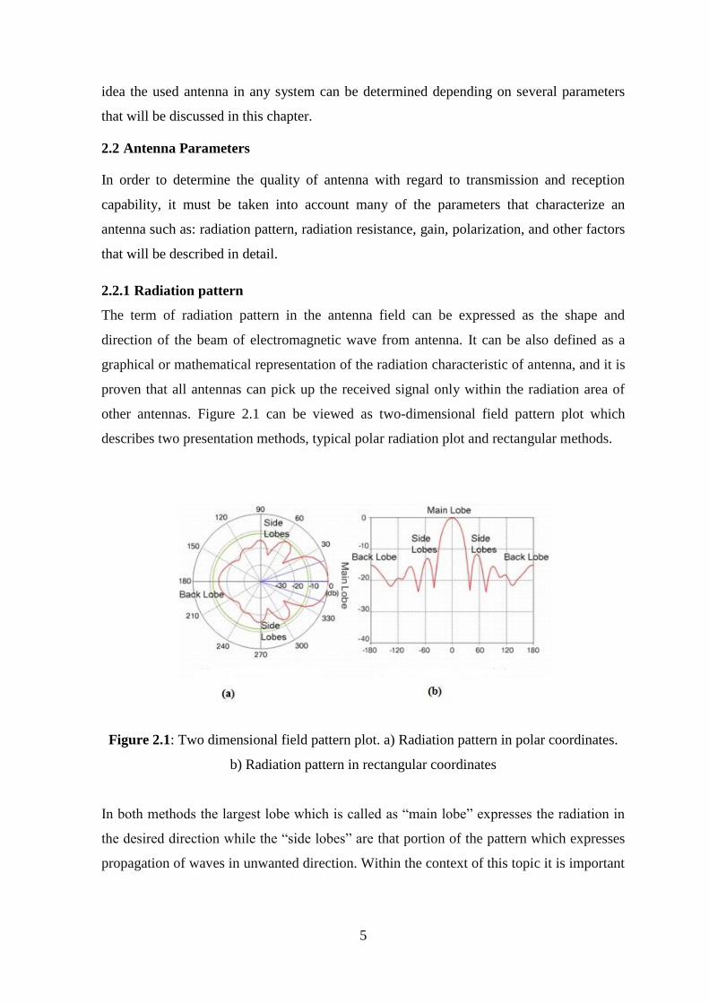
2.2.1 Radiation pattern
The term of radiation pattern in the antenna field can be expressed as the shape and
direction of the beam of electromagnetic wave from antenna. It can be also defined as a
graphical or mathematical representation of the radiation characteristic of antenna, and it is
proven that all antennas can pick up the received signal only within the radiation area of
other antennas. Figure 2.1 can be viewed as two-dimensional field pattern plot which
describes two presentation methods, typical polar radiation plot and rectangular methods.
Figure 2.1: Two dimensional field pattern plot. a) Radiation pattern in polar coordinates.
b) Radiation pattern in rectangular coordinates
In both methods the largest lobe which is called as “main lobe” expresses the radiation in
the desired direction while the “side lobes” are that portion of the pattern which expresses
propagation of waves in unwanted direction. Within the context of this topic it is important
6
to mention to beamwidth of lobe which demonstrate the capability of antenna to
distinguish between two different sources of radiation, (Khasim, Krishna, & Thati.).
2.2.2 Antenna gain
Among the many parameters that characterize antennas, this is the most effective
expression of antenna performance characteristic, which is defined by the wireless
communications terms as the ability of antenna to direct energy in particular direction, and
it is an indication of the directivity of the directional Antenna feature, typically the
measurement of antenna gain is measured in dB (Fonda & Zennaro, 2004). It is also
observed that when the antenna has a high gain, it leads to narrower beamwidth, and that
means fewer opportunities to receive interference. Oppositely, the antenna with the low-
gain has the highest chances to receive interference due to the wide beam width.
2.2.3 Bandwidth
In the manufacturing stage of antennas, the broad band of antenna is determined. This
characteristic indicates to the frequencies band that can be sent or received by antenna.
The bandwidth of an antenna usually described in two different way, the first method
expresses the bandwidth of the antenna in absolute unit of frequency, while other method
can describe this term with reference to the center of frequency band. This can be
illustrated by the equation:
BW = 100 × (FH − FL) / FC
Where:
FH is the highest frequency in the frequency band.
FL is the lowest frequency in the frequency band.
FC is the center frequency in the frequency band.
2.2.4 Polarization
This parameter is one of the fundamental characteristics of antenna; it refers to the
direction of the radiated electric field of the electromagnetic wave, which is produced by
antenna. Hence, antennas are categorized as "Linearly Polarized", "Circularly Polarized
Antenna", and “elliptically polarized antenna”. If the magnetic and electric field
perpendicular in respect to the plane wave and travelling in a signal direction, the electric
field would be a Linear polarization, while if the field rotates in circle, this field would be
said to be circularly polarized .However, if the electric field has two components that are
perpendicular and out of phase but are not equal in magnitude, the E-field could be
7
considered as elliptical polarized. Due to the reciprocity theorem, both transmitter and
receiver antenna should be in the same polarity and thus there would be no loss of energy
because of polarization mismatch. In another words, if the polarization of the transmitter is
vertical while receiver antenna is horizontally polarized, the energy will not be
transferred.(Boyle & Huang, 2008)
2.3 Antenna Classification
According to the antenna radiation, it can be classified into several types, including
isotropic, omnidirectional and directional antenna .Whereas they can be categorized
depending on their functions and operation to phased antenna array and adaptive antenna
array.
2.3.1 Isotropic antenna
An isotropic radiator radiates the energy in all direction with equal intensity, Therefore, is
considered as a theoretical ideal reference in electromagnetic waves laboratory in order to
make comparisons with other types of antennas.
2.3.2 Omni directional antennas
This type of antenna is the most commonly used in wireless communication systems such
as FM radio and radio broadcasting because it has the ability to receiving and radiating
energy in all directions equally. Therefore; it can be said that it is non-directional antenna,
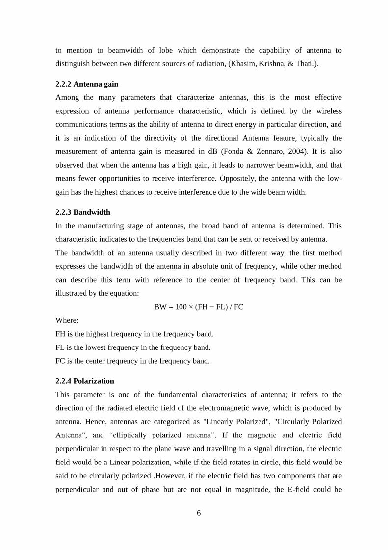
and this is evident in the radiation pattern shown in figure 2.2. Despite the ability to
broadcast the signal in 360 coverage directional, this feature leads to many bad
consequences for wireless communication systems. The most prominent problems that are
facing this type of antenna is inability to reject interference because it can’t send
information to users directionally. Wherefore, it does not achieve the expected benefit in
increasing Capacity and SIR for signal. (Fung, 2011)In addition , the most types of omni-
directional antennas Can be considered as low gain antennas because they radiate the wave
indirectly manner and it affects the quality of service .Thus the use of this type of antennas
imposes a lot of restrictions on wireless communications systems, especially in the field of
capacity, service quality, Powered Control ,coverage and frequency reuse. This behavior in
non-directed broadcasts scatters signals and reduces the percentage of energy that reaches
the desired user. Therefore, the designers solving this problem by increasing the power
level of antenna broadcast, but this has made the situation worse because of the high
8
chance of interference with co-channels in neighboring cells that operate in same set of
frequencies(Antenna Basic Concepts).
Figure 2.2: Coverage pattern for omni-directional antenna
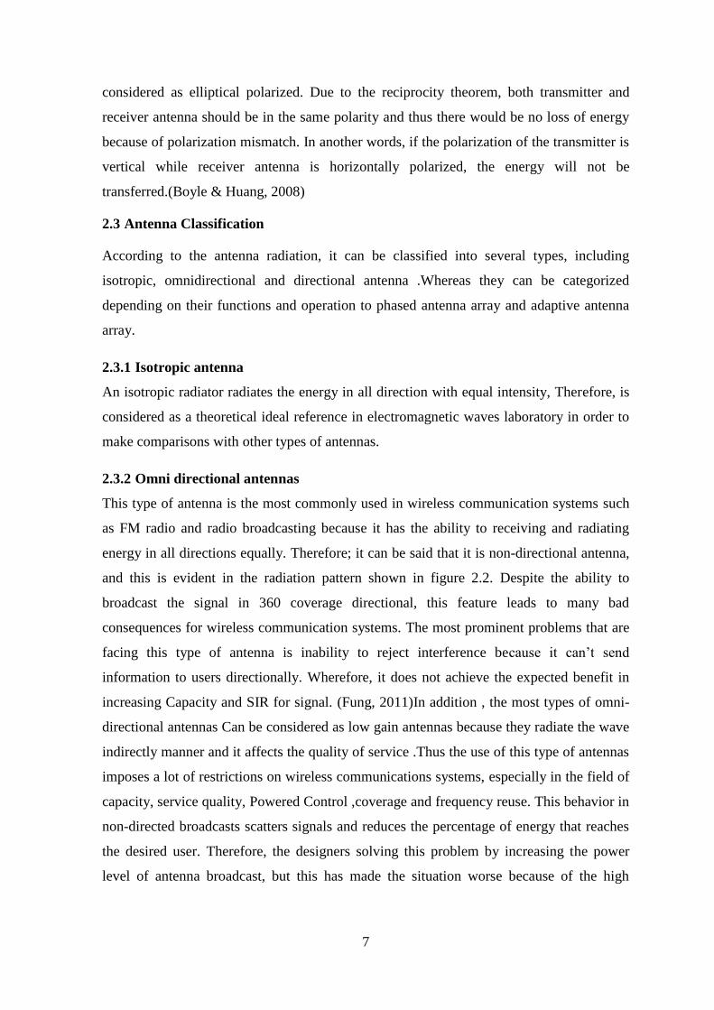
2.3.3 Directional Antennas
With the development of communication it was necessary to find a solution leading to raise
the antenna efficiency without polluting the environment with interferences ,this is what
led to the adoption of directed antenna which can be defined as a device capable of
transmitter and receiver the power in a particular directions by directing a narrow
beamwidth of signal toward the target, this behavior raises the antenna performance by
increasing the gain and makes it capable of reducing the proportion of receiving
interference .
Figure 2.3: Coverage pattern for Sectorized antenna system
9
2.3.4 Antenna array
In order to overcome the drawbacks facing the conventional antennas in terms of inability
to reject interference, the antenna array system came to be the solution, and generally fall
in two categories.
2.3.4.1 Phased array
The phased array consists of several elements of radiation are arranged and linked in a
certain way to give direction radiation model. This Array has wide applications in radar,
communications, and at the present time in the microwave frequencies used in satellite
communications, the main objective of this technique is to increase gain in the desired
direction and suppression the radiation in the unwanted direction, by adjusting the phases
of the signals that feed input elements in array. For illustration purposes it can be said that
the total electromagnetic field of an array is obtained by vector addition of the fields
emitted by the array elements, combined in both phase and amplitude. (Balanis &
Ioannides, Introduction to smart antenna, 2007)
2.3.4.2 Adaptive array
In communication terms the “adaptive array” refers to the radiation properties of array
which is characterized by its ability to change the radiation depending on changes and
requirements of system, this array is distinct from traditional antennas through its ability to
operate with high performance in dynamic environments which features that signals
whether desired or unwanted arrive from different directions and different levels of energy.
In addition, the use of adaptive arrays in communication system would provide reliability
and better quality compared to the conventional systems, through the ability to reduce the
level of side lobes in the direction of unwanted signals and reduce the interference while
maximize the radiation pattern toward the desired user(Balanis & Ioannides, Introduction
to smart antenna, 2007) .This adaptive technique which adopted by this array is mainly
carried out through signal processing unit which improve the performance by adapting the
weights based on the received signal in order to maximize reception in the desired
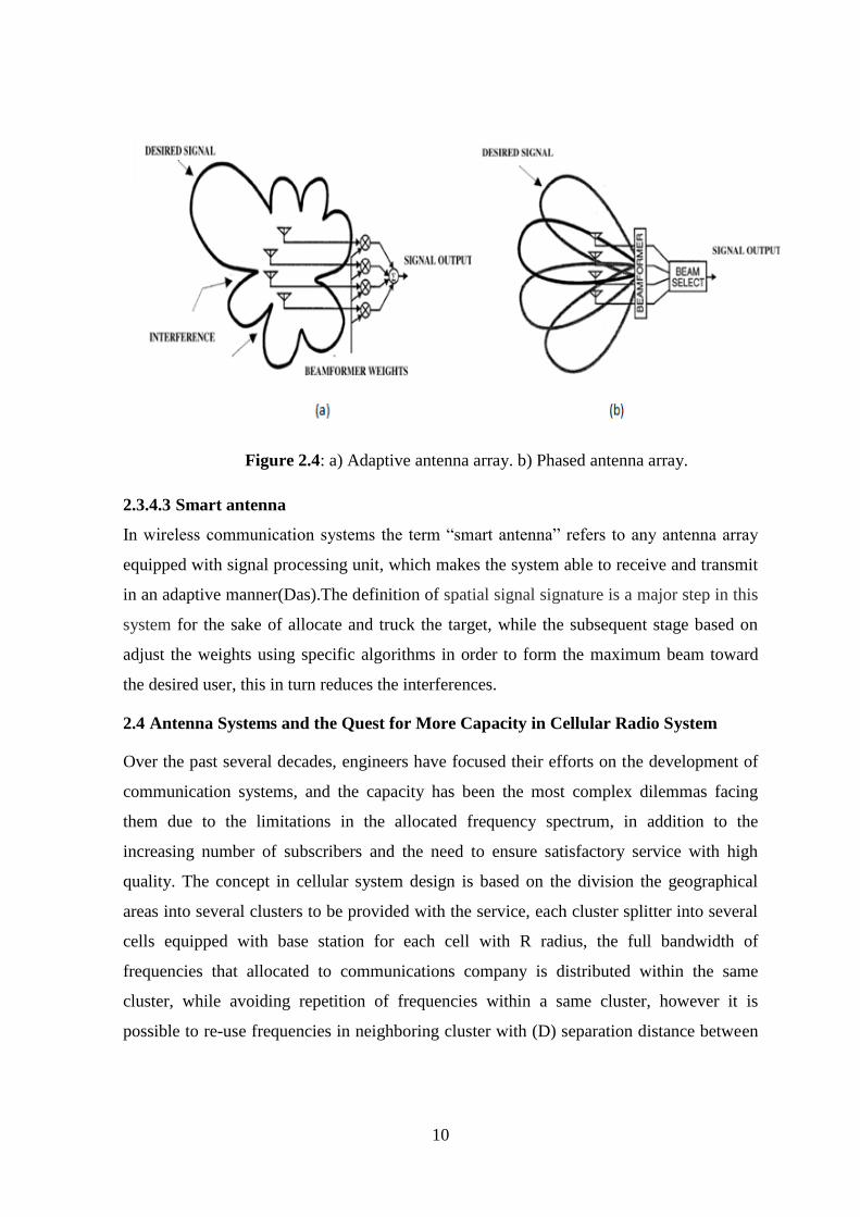
direction and minimize the reception from unwanted users. Figure 2.4 illustrates the
difference between the two antenna array techniques, where it is clear that adaptive array
technique has ability to achieve better performance, which would ensure the suppression of
interferences entirely.
10
Figure 2.4: a) Adaptive antenna array. b) Phased antenna array.
2.3.4.3 Smart antenna
In wireless communication systems the term “smart antenna” refers to any antenna array
equipped with signal processing unit, which makes the system able to receive and transmit
in an adaptive manner(Das).The definition of spatial signal signature is a major step in this
system for the sake of allocate and truck the target, while the subsequent stage based on
adjust the weights using specific algorithms in order to form the maximum beam toward
the desired user, this in turn reduces the interferences.
2.4 Antenna Systems and the Quest for More Capacity in Cellular Radio System
Over the past several decades, engineers have focused their efforts on the development of
communication systems, and the capacity has been the most complex dilemmas facing
them due to the limitations in the allocated frequency spectrum, in addition to the
increasing number of subscribers and the need to ensure satisfactory service with high
quality. The concept in cellular system design is based on the division the geographical
areas into several clusters to be provided with the service, each cluster splitter into several
cells equipped with base station for each cell with R radius, the full bandwidth of
frequencies that allocated to communications company is distributed within the same
cluster, while avoiding repetition of frequencies within a same cluster, however it is
possible to re-use frequencies in neighboring cluster with (D) separation distance between
11
two cells that have the same set of frequencies. Because of this way of frequency
allocation, interference occurs and this is called co –channel interference.
In the past decades omni-directional antenna has been used in base station which led to
pollute the environment with interference, this caused the concentration of efforts to find a
solution through the replacement of omni-directional antenna system with systems called
“sectorized system”, In this case the cell is divided into three or six sections by replacing
the omni-directional antenna with several directional antennas and this technique called
“cell sectoring”, and thus reduces the number of co-channel cells within the likely range
for the occurrence of interference(Goldsmith, 2004).
cellular design technique depends on increasing capacity by decreasing the number of cells
in cluster, decreasing the radius of cell R, or decreasing the distance D and thus the re-use
frequency would increase to achieve an increase in capacity(Bellofiore, Balanis, Foufz, &
Spanias, Smart-Antenna Systems for Mobile communication network, 2002). One of the
technique has followed to improve capacity is “cell splitting “which relies on reducing
energy that transmitted by antenna through the principle of the division of the cell into
microcell and each small cell equipped with it is own omni-directional antenna in base
station, where the full bandwidth is distributed within the splitted cell. In this way, the
number of cells increases, thereby increasing the possibility of re-uses frequencies which
lead to raise the capacity. Although it considered one of the methods that led to increase
capacity, the design of this system is expensive due to the need for more base stations. This
resulted in the quest for finding other solutions to the capacity.
12
CHAPTER 3
SMART ANTENNA SYSTEM
Over decades, designers and developers of wireless communications systems have been
seeking continuously to overcome the obstacles facing the systems, co-channel
interferences, multipath fading and inter-symbol-interference (ISI) are considered as main
problems that lead to the decline in the quality of service and limit the numbers of
subscribers served by system (Jain, Katiyar, & Agrawal, 2011)
Co-channel interference refers to the interference that occurs when signals that have same
frequency reach to the receiver, where one of these signals is the desired, and the rest are
unwanted signals due to the frequency reuse principle which depends on reassigning the
same spectrum bands to other distant cells (The cellular concept-system design
fundamental, 2002).Despite that omni-directional antenna systems provide high coverage
due its in-directional radiation, however it leads to increase co-channel interferences.
The reliance on traditional systems such as omni-directional and diversity system has been
shown that these solutions are not satisfactory to the growing demands for wireless
systems as well as the need to reduce infrastructure and maintenance costs. On the other
hand the performance of system is also affected and getting worse due to the interference
caused by the reception of the signal from several tracks which is called multipath fading,
only smart antenna system, which has passed through several stages of development before
becoming commercial, exploit the problem of receiving the signal from different directions
to improve reception by directions spatial processing that distinguishes this system(Azad &
Ahmed, 2010). Wherefore recent research has concentrated on the development of
algorithms that used in the design of “smart antenna system” which has the ability to
develop various aspects of wireless communications systems including power control,
quality of services and capacity. This system was able to outperform conventional systems
in terms of spectral efficiency by achieving more capacity so that a larger number of
subscribers can be served ,in addition to acquire greater coverage areas and raise the
performance in terms of data rate.
In this chapter the concept of smart antenna and its types will be presented, the
architectures of system will be described as well as the most important benefits,
advantages, drawbacks of this system and its applications in communication field.
13
3.1 Smart Antenna System Concept
Smart antenna system is defined as a combination of elements constitute the hardware
section which are also called antenna array, while the software part is represented by the
digital signal processing unit that makes the system intelligent (Jain, Katiyar, & Agrawal,
2011).Over the last few years the research has tended to develop algorithms that give the
system the ability to identify ,locate and truck user dynamically via DOA and Adaptive
algorithms, in order to direct the main beam towards the desired target and nulls in
unwanted directions via beamforming algorithms this would significantly reduce the noise
and maximize the directivity of antenna (Bellofiore, Balanis, Foufz, & Spanias, Smart-
Antenna Systems for Mobile for communication networks, 2002).
In other word, smart antenna system can be defined as a smart technology that can increase
the gain of antenna array system which in turn reduces interferences, thus increases the
quality of service and performance of the system, and the spectral efficiency is achieved.
3.1.1 Analogy for adaptive smart antenna
The human brain is often regarded as a source of inspiration for many intelligent systems
that are trying to approximating the systems of the human, and that was the case with smart
antenna system.
Scientists have observed that a human is able to identify and locate the desired sound as
well as focus on it, even in the presence of other voices or sound source movement. This
property is due to the presence of ears, which receive the vote with a time delay due to
spatial difference between them, thus it can be said that ears are similar to the radiation
elements in an antenna array while the brain act as a software part in smart antenna system
through its calculation process for determining the direction of the desired speaker from
the delay time that received by the two ears (Balanis & Ioannides, Introduction to Smart
Antennas, 2007). Therefore, a person can locate and truck the interest speaker in dark room
and suppress any other noise voices through this system which consists of two ears and the
brain, which is equivalent to performance of smart antenna system that can transmits and
receives signals in adaptive spatially manner and has the ability to maximize the reception
toward the target while minimize the interfering signals. Figure 3.1 below illustrates the
analogy for Adaptive Smart Antenna through blindfolded man in a dark room and two
speakers.
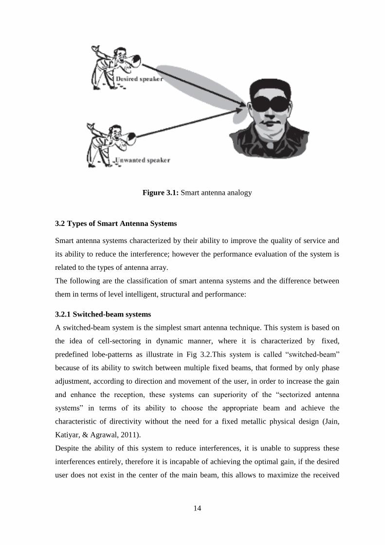
14
Figure 3.1: Smart antenna analogy
3.2 Types of Smart Antenna Systems
Smart antenna systems characterized by their ability to improve the quality of service and
its ability to reduce the interference; however the performance evaluation of the system is
related to the types of antenna array.
The following are the classification of smart antenna systems and the difference between
them in terms of level intelligent, structural and performance:
3.2.1 Switched-beam systems
A switched-beam system is the simplest smart antenna technique. This system is based on
the idea of cell-sectoring in dynamic manner, where it is characterized by fixed,
predefined lobe-patterns as illustrate in Fig 3.2.This system is called “switched-beam”
because of its ability to switch between multiple fixed beams, that formed by only phase
adjustment, according to direction and movement of the user, in order to increase the gain
and enhance the reception, these systems can superiority of the “sectorized antenna
systems” in terms of its ability to choose the appropriate beam and achieve the
characteristic of directivity without the need for a fixed metallic physical design (Jain,
Katiyar, & Agrawal, 2011).
Despite the ability of this system to reduce interferences, it is unable to suppress these
interferences entirely, therefore it is incapable of achieving the optimal gain, if the desired
user does not exist in the center of the main beam, this allows to maximize the received
15
power of the interference that is located in the center of the same fixed beam more than the
desired target. (Bellofiore, Balanis, Foufz, & Spanias, 2002).
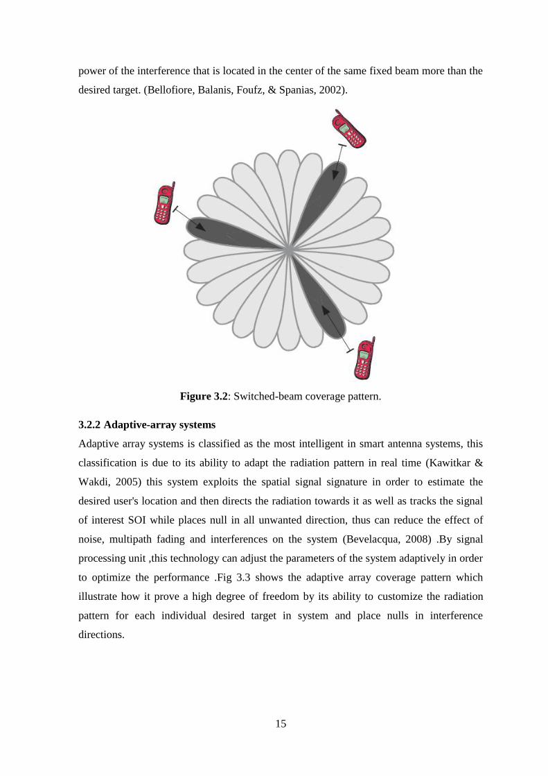
Figure 3.2: Switched-beam coverage pattern.
3.2.2 Adaptive-array systems
Adaptive array systems is classified as the most intelligent in smart antenna systems, this
classification is due to its ability to adapt the radiation pattern in real time (Kawitkar &
Wakdi, 2005) this system exploits the spatial signal signature in order to estimate the
desired user's location and then directs the radiation towards it as well as tracks the signal
of interest SOI while places null in all unwanted direction, thus can reduce the effect of
noise, multipath fading and interferences on the system (Bevelacqua, 2008) .By signal
processing unit ,this technology can adjust the parameters of the system adaptively in order
to optimize the performance .Fig 3.3 shows the adaptive array coverage pattern which
illustrate how it prove a high degree of freedom by its ability to customize the radiation
pattern for each individual desired target in system and place nulls in interference
directions.
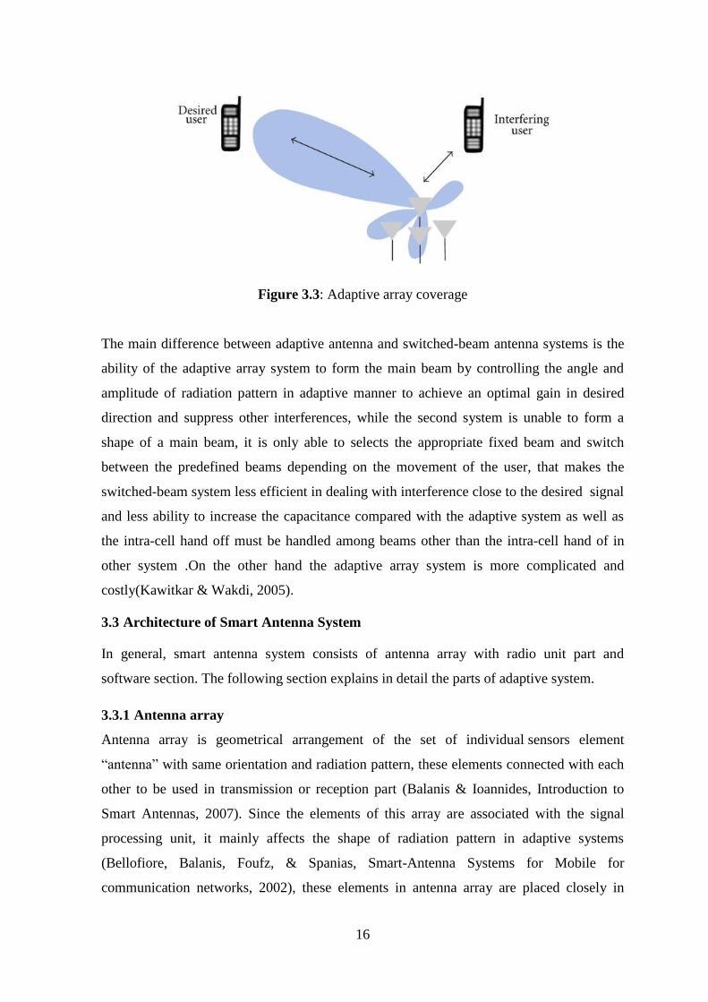
16
Figure 3.3: Adaptive array coverage
The main difference between adaptive antenna and switched-beam antenna systems is the
ability of the adaptive array system to form the main beam by controlling the angle and
amplitude of radiation pattern in adaptive manner to achieve an optimal gain in desired
direction and suppress other interferences, while the second system is unable to form a
shape of a main beam, it is only able to selects the appropriate fixed beam and switch
between the predefined beams depending on the movement of the user, that makes the
switched-beam system less efficient in dealing with interference close to the desired signal
and less ability to increase the capacitance compared with the adaptive system as well as
the intra-cell hand off must be handled among beams other than the intra-cell hand of in
other system .On the other hand the adaptive array system is more complicated and
costly(Kawitkar & Wakdi, 2005).
3.3 Architecture of Smart Antenna System
In general, smart antenna system consists of antenna array with radio unit part and
software section. The following section explains in detail the parts of adaptive system.
3.3.1 Antenna array
Antenna array is geometrical arrangement of the set of individual sensors element
“antenna” with same orientation and radiation pattern, these elements connected with each
other to be used in transmission or reception part (Balanis & Ioannides, Introduction to
Smart Antennas, 2007). Since the elements of this array are associated with the signal
processing unit, it mainly affects the shape of radiation pattern in adaptive systems
(Bellofiore, Balanis, Foufz, & Spanias, Smart-Antenna Systems for Mobile for
communication networks, 2002), these elements in antenna array are placed closely in
17
order that there will be no differences in amplitude of the received signals and the number
of antennas must be the minimum number of required for designed system in order to
avoid complexity.
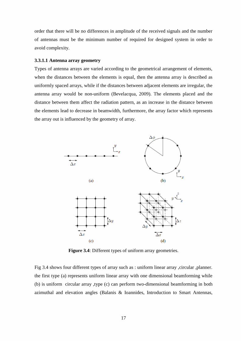
3.3.1.1 Antenna array geometry
Types of antenna arrays are varied according to the geometrical arrangement of elements,
when the distances between the elements is equal, then the antenna array is described as
uniformly spaced arrays, while if the distances between adjacent elements are irregular, the
antenna array would be non-uniform (Bevelacqua, 2009). The elements placed and the
distance between them affect the radiation pattern, as an increase in the distance between
the elements lead to decrease in beamwidth, furthermore, the array factor which represents
the array out is influenced by the geometry of array.
Figure 3.4: Different types of uniform array geometries.
Fig 3.4 shows four different types of array such as : uniform linear array ,circular ,planner.
the first type (a) represents uniform linear array with one dimensional beamforming while
(b) is uniform circular array ,type (c) can perform two-dimensional beamforming in both
azimuthal and elevation angles (Balanis & Ioannides, Introduction to Smart Antennas,
18
2007), last one is a cubic array with separation of Δ x, Δ y, and Δ z. this structural is
conceder as three dimensional array.
3.3.1.2 Theoretical model for an antenna array
The first mathematical rule that must be considered when designing the smart antenna
design is the distance between the elements in uniform array, which likes to be constrained
by the following law:
2
d
(3.1)
Where d is the distance between two adjacent antennas and is the wavelength, if the
separation distance is greater than the half-wavelength then the grating lobes will occur,
this term is refers to the sidelobe which has considerable amplitude with respect to main
lobe and possibly up to its amplitude value (Bevelacqua, 2008), however this phenomenon
is difficult to be controlled if the array is non-uniform.
Assuming ULA with N =5 elements smart antenna vector receiving three signal s1, s2, and
s3; the steering vector defines the angle in which each one of the signal is received by each
element of the antenna. The angle of one of the elements is considered as reference and the
other elements angles are calculated as follow (supposing d=0.5λ).
2 2sin ( 1) sin
( ) [1, ,....., ]d d
j j NTa e e
(3.2)
1 1 1 1
2 2 2 2
3 3 3 3
2 sin( ) sin( ) sin( ) 2 sin( )
1
2 sin( ) sin( ) sin( ) 2 sin( )
2
2 sin( ) sin( ) sin( ) 2 sin( )
3
1
1
1
s s s s
s s s s
s s s s
Tj kd jkd jkd j kd
S
Tj kd jkd jkd j kd
S
Tj kd jkd jkd j kd
S
a e e e e
a e e e e
a e e e e
(3.3)
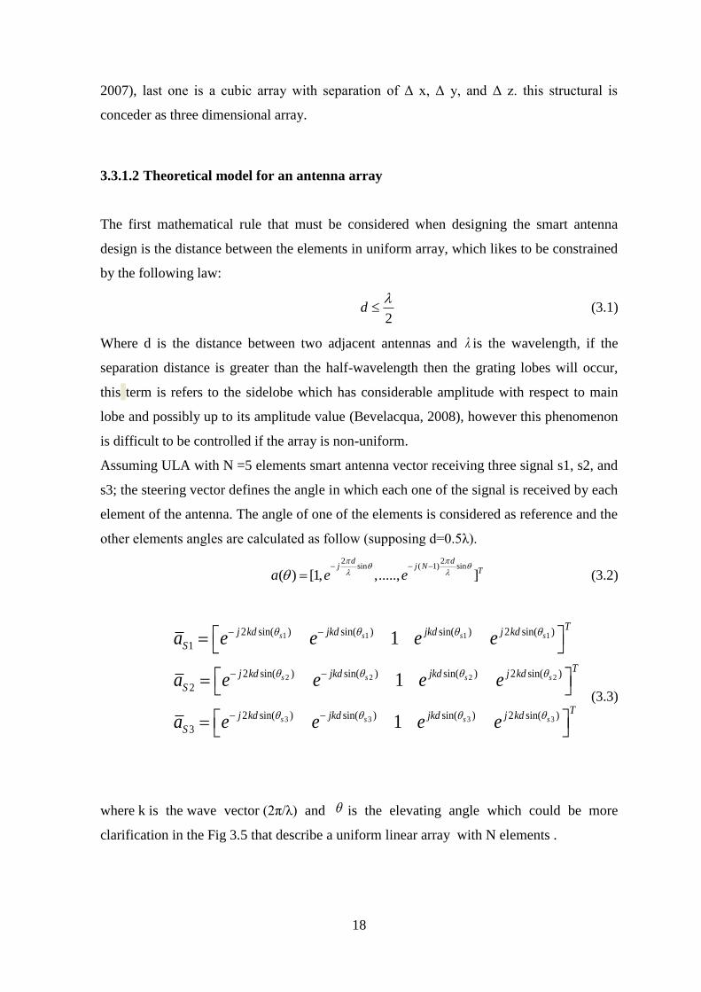
where k is the wave vector (2π/λ) and is the elevating angle which could be more
clarification in the Fig 3.5 that describe a uniform linear array with N elements .
19
Figure 3.5: ULA with N sensors
By adjusting the weights and determine the array geometry, the system can achieve the
optimal radiation and reception in desired direction while suppress the interferences from
unwanted direction, and this idea can be expressed mathematically through the array factor
equation, this term is a function of separation distance in array, their relative phase and
magnitude as well as the weights used (Bevelacqua, The Array Factor, 2009).the array
factor is given by:
1
( )N
i
i
AF a
(3.4)
Where
i is complex array weight at element i.
is angle of incidence of electromagnetic plane wave from array axis.
N is the number of elements in antenna array.
a is steering vector.
3.3.2 Radio unit (hardware)
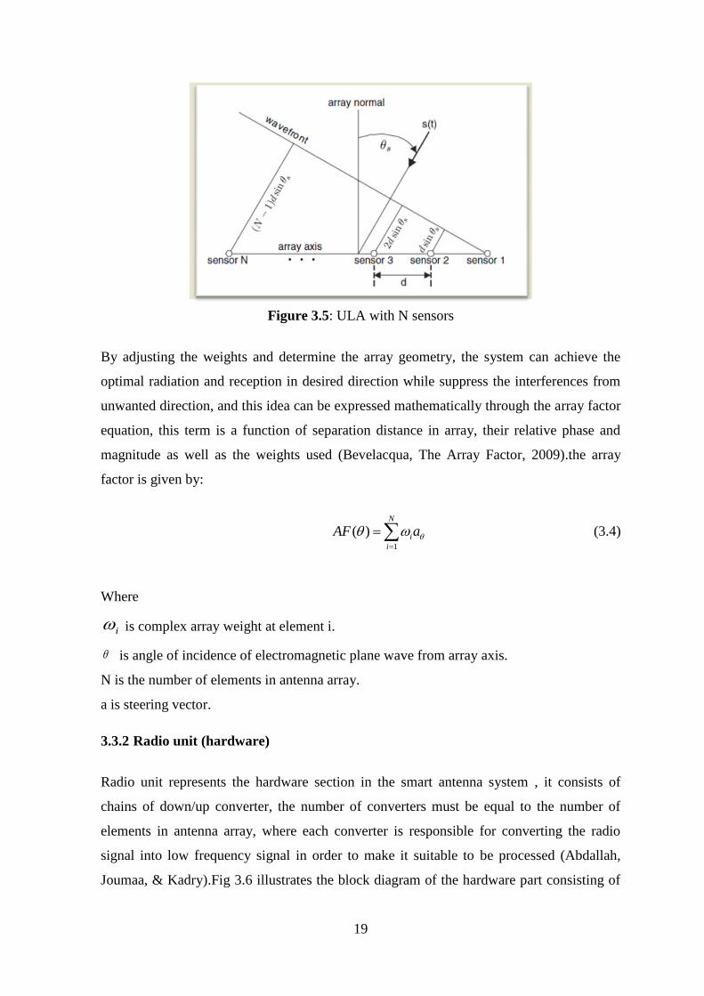
Radio unit represents the hardware section in the smart antenna system , it consists of
chains of down/up converter, the number of converters must be equal to the number of
elements in antenna array, where each converter is responsible for converting the radio
signal into low frequency signal in order to make it suitable to be processed (Abdallah,
Joumaa, & Kadry).Fig 3.6 illustrates the block diagram of the hardware part consisting of
20
antennas elements that receive signals and then injects the signals into low-noise amplifier
which is responsible of amplifying a very low-power signal without changing its signal-to-
noise ratio. Second part in hardware is down/up converter and the last one is analog-to-
digital block which digitize the signal to be Prepared to the digital signal processing stage.
Figure 3.6: The hardware part in smart antenna (receiving section)
3.3.3 Signal processing unit
In Adaptive system, signal processing unit has the main role in enhancing the performance
efficiency and make it an intelligent system. In this unit, the information is collected in
order to extract the knowledge and applied through adaptive Signal-Processing algorithms
(Bellofiore, Foutz, Balanis, & Spanias, 2002), furthermore, signal processing is responsible
for identifying the location of the signal after it is captured and trucking it in order to
maximize the reception in interest direction and filtering out the interferences from
unwanted direction. This process is done by direction-of-arrival estimator (DOA estimator)
and adaptive beam-forming.
3.3.3.1 DOA estimator
Direction of arrival estimation is refers to the technique that estimate the analog arrival of
received signals from the time delays for each elements in the array and includes a
correlation analysis of the array signals followed by Eigen analysis and signal noise sub-
space formation (Bellofiore, Foutz, Balanis, & Spanias, 2002).The goal of AOA estimation
techniques is to define a function that gives an indication of the angles of arrival based
upon maxima vs. angle. This function is traditionally called the pseudo spectrum P (θ) and
the units can be in energy or in watts (or at times energy or watts squared). There are
21
several potential approaches to defining the pseudo-spectrum .In general, the DOA
estimation algorithms can be categorized into several groups; the conventional techniques,
subspace techniques, maximum likelihood techniques and integrated techniques(Joseph
C.Libertii & S.Rappaport, 1999).
3.3.3.2 Adaptive beamformer
The most essential process in smart antenna system is beam forming, which it is also refer
to spatial filter, since it has the ability to filter signals based on their spatial direction.
Hence, the signal not of interest (SNOI) is filtered out while the signal of interest (SOI) is
amplified (Stevanovic, Skrivervik, & Mosig, 2003).This spatial processing technique
depends on the information that has been obtained from the previous steps from DOA
estimator, in order to shape the beam pattern of an antenna array and nullify the signals in
unwanted directions, this continuously changes process is done by adjusting and
computing the optimal complex weight vector via adaptive algorithms. Thus, the
performance efficiency of smart antenna system gets increased as well as the signal-to-
noise ration. Algorithms and adaptive beamforming technique will be explained later in
chapter 4.
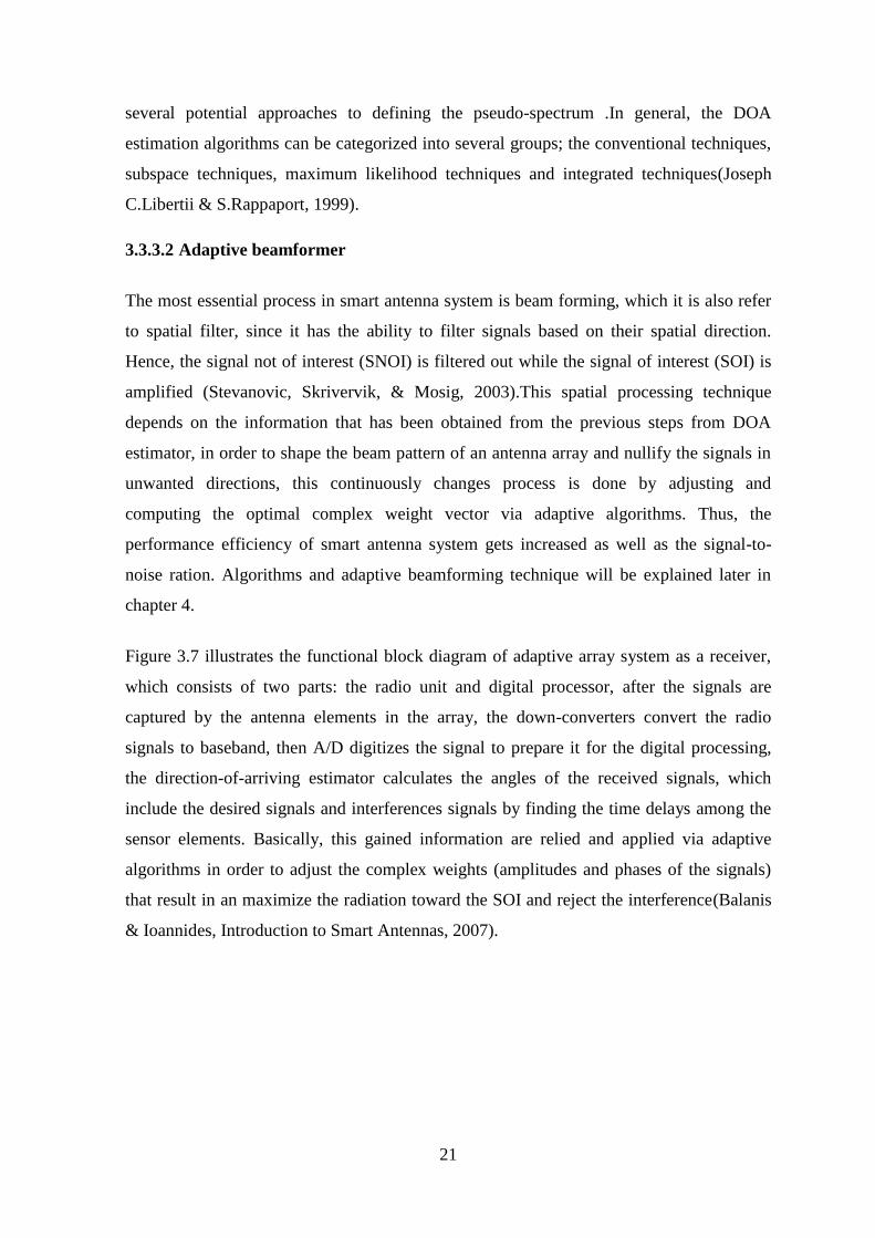
Figure 3.7 illustrates the functional block diagram of adaptive array system as a receiver,
which consists of two parts: the radio unit and digital processor, after the signals are
captured by the antenna elements in the array, the down-converters convert the radio
signals to baseband, then A/D digitizes the signal to prepare it for the digital processing,
the direction-of-arriving estimator calculates the angles of the received signals, which
include the desired signals and interferences signals by finding the time delays among the
sensor elements. Basically, this gained information are relied and applied via adaptive
algorithms in order to adjust the complex weights (amplitudes and phases of the signals)
that result in an maximize the radiation toward the SOI and reject the interference(Balanis
& Ioannides, Introduction to Smart Antennas, 2007).
22
Figure 3.7: Functional block diagram (adaptive array system)
3.4 The goal of smart antenna
Smart antenna system has achieved a quantum leap in communications world because of
the solutions that provided by this system, in addition to its features that make it superior to
other traditional wireless systems.
Increasing the coverage
Coverage area is refers to the area where the communication between a user and the base
station is available, because smart antennas is more directive than convention systems such
as omnidirectional antennas or sectoring systems ,it can achieve better coverage. This
feature significantly associated with higher gain that is provided by the adaptive system.
Moreover, it has been proved that this smart system achieves coverage greater by (M) than
conventional systems, while the number of required base station has decreased by (1/M) by
using smart antenna system with M antenna elements (Sallomi & Salim, 2009).it worth
mentioning that the directivity characteristic of smart antenna system impacts on mobile
devices through minimize the required level of power and thus prolonging battery life
(Bellofiore, Balanis, Foufz, & Spanias, Smart-Antenna Systems for Mobile for
communication networks, 2002)
23
Increasing capacity
Adaptive array system is able to meet the growing need for capacity by being able to
radiates and receives in desired direction while suppress the interference or noise that
affect on the service and limit the possibility of re-use of frequency. Interference rejection
feature enables the system to increase the signal-to-interference ratio which in turns
increase the capacity, thus increasing the number of subscriber in designed
system(Bellofiore, Balanis, Foufz, & Spanias, Smart-Antenna Systems for Mobile for
communication networks, 2002)
Increasing bit-rate
Depending on the spatial variation of the signals, the system can exploit this feature to
reject signals coming from multiple paths, which cause multipath fading and ISI
(Stevanovic, Skrivervik, & Mosig, 2003).Instead of using the equalizer to recover the
signal, adaptive array system is used in order to reduce the delay spread of the channel and
that would reject multipath and support the bit rate.
Security
The security feature is considered a necessary issue in the field of communications to avoid
intruding on users network data, the solution provided by the smart antenna lies in its
ability to radiate in adaptive manner with high gain; thus, the transmission of signals is not
in all directions and thereby reducing the probability of spying on data and increase
security whereas the hacker must be in the same location of the users (Balanis & Ioannides,
Introduction to Smart Antennas, 2007).
3.5 The drawbacks
Despite the many benefits realized by the smart antenna system, many of the problems
facing this system and make it difficult to apply in some application.
Complexity
The operations performed by the system on the receiving signals in order to optimize the
service quality affect on the system and make it more complicated, especially in terms of
the separation of incoming signals and synchronize them with real-time(Balanis &
Ioannides, Introduction to Smart Antennas, 2007). In addition to the base station
requirements to high-resolution powerful processors and controllers, this makes the system
more complicated because of the need for complex mathematical operations in digital
signal processing part.

24
Size
The need to increase the number of elements in antenna array to provide better
performance in addition to the fact that the separation distance between them restricted on
condition (2
d
) and is depending on the operator frequency, lead to an increase in
antenna array size, for example, the antenna array size would be approximately 1.2 meters
wide at a frequency of 900 MHz and 60 cm at 2 GHz (Balanis & Ioannides, Introduction to
Smart Antennas, 2007).
25
CHAPTER 4
BEAMFORMING ALGORITHMS
Adaptive Smart antenna structure is distinguished by the capability to form and object the
radiation of the main beam in the direction of the desired user with eliminating the non
desired signals and noise. This is used to increase the performance during the transmission
and reception of communication signal.This technique, which constitute the array beam
pattern is referred as the beam forming.
In this chapter, the fundamentals of fixed weight beam forming will be presented in
addition to the adaptive beam forming strategies and then we will review some of the
adaptive beam forming algorithms used in the system, which will be simulated to discuss
the results in next chapter.
4.1 Fixed Weight Beam-forming Basics
Beam forming techniques are basically classified into two main approaches, the fixed
weight beam forming and adaptive beam forming (Cohen, 2003). The former term refers to
the process by which weights are fixed and the incoming signal does not change with the
times, and thus the optimum weights is not based on the received data and won’t need to be
adjusted (Gross, 2005). In order to get the optimal weight we can follow several methods
such as SIR, LM methods and MV that will be explained in the following sections.
4.1.1 Maximum signal-to-interference ratio approach
SIR can be known as the ratio between the power of wanted signal to that of undesired
signal (Gross, 2005). This ratio indicates that the increase in SIR will lead to improve
signal reception and reduce interference.
26
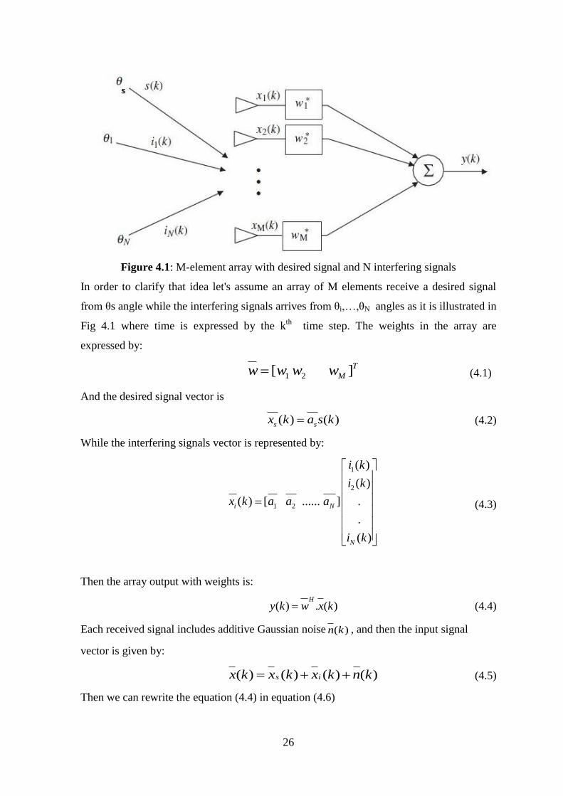
Figure 4.1: M-element array with desired signal and N interfering signals
In order to clarify that idea let's assume an array of M elements receive a desired signal
from θs angle while the interfering signals arrives from θi,…,θN angles as it is illustrated in
Fig 4.1 where time is expressed by the kth
time step. The weights in the array are
expressed by:
1 2[ ]T
Mw w w w (4.1)
And the desired signal vector is
( ) ( )s sx k a s k (4.2)
While the interfering signals vector is represented by:
1
2
1 2
( )
( )
( ) [ ...... ] .
.
( )
i N
N
i k
i k
x k a a a
i k
(4.3)
Then the array output with weights is:
( ) . ( )H
y k w x k (4.4)
Each received signal includes additive Gaussian noise ( )n k , and then the input signal
vector is given by:
( ) ( ) ( ) ( )s ix k x k x k n k (4.5)
Then we can rewrite the equation (4.4) in equation (4.6)
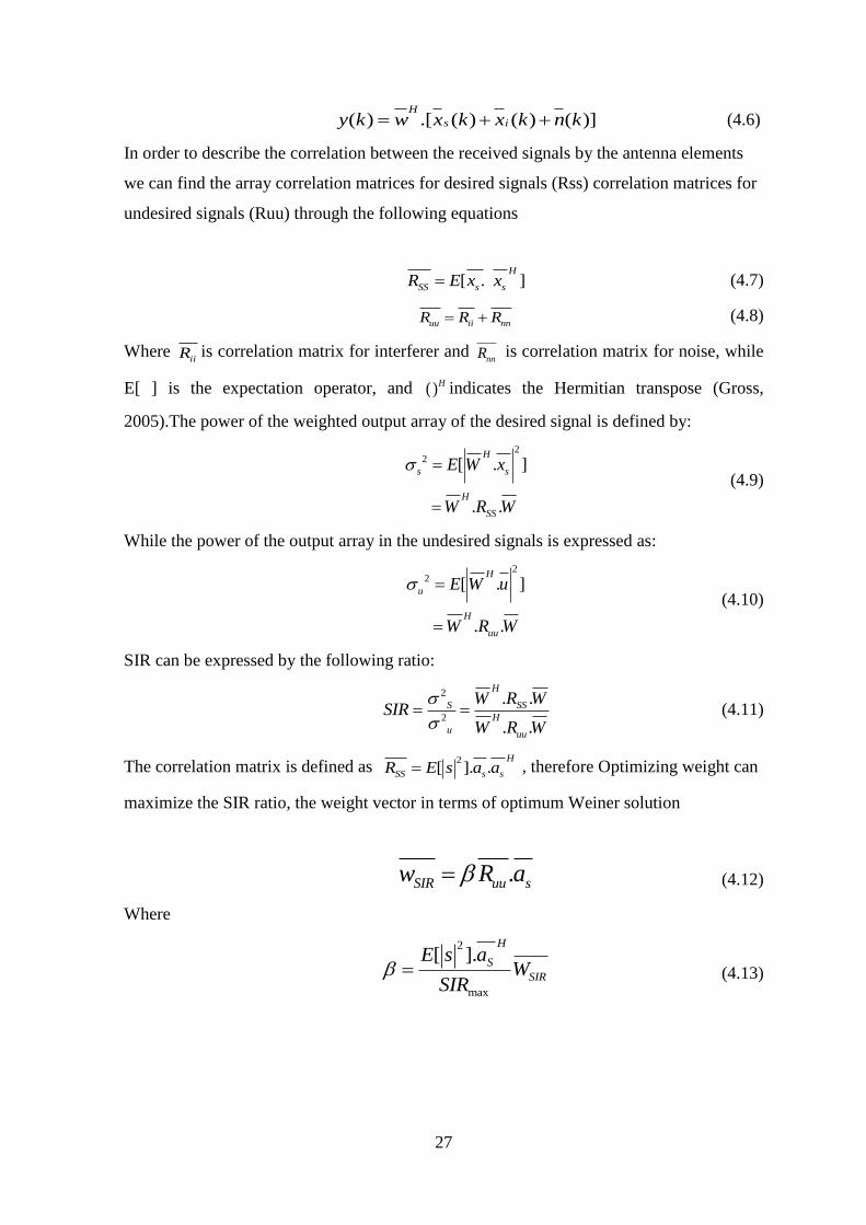
27
( ) .[ ( ) ( ) ( )]H
s iy k w x k x k n k (4.6)
In order to describe the correlation between the received signals by the antenna elements
we can find the array correlation matrices for desired signals (Rss) correlation matrices for
undesired signals (Ruu) through the following equations
[ . ]H
SS s sR E x x (4.7)
uu ii nnR R R (4.8)
Where iiR is correlation matrix for interferer and
nnR is correlation matrix for noise, while
E[ ] is the expectation operator, and ( )H indicates the Hermitian transpose (Gross,
2005).The power of the weighted output array of the desired signal is defined by:
22 [ . ]
. .
H
s s
H
SS
E W x
W R W
(4.9)
While the power of the output array in the undesired signals is expressed as:
22 [ . ]
. .
H
u
H
uu
E W u
W R W
(4.10)
SIR can be expressed by the following ratio:
2
2
. .
. .
H
S SS
H
u uu
W R WSIR
W R W
(4.11)
The correlation matrix is defined as 2
[ ]. .H
SS s sR E s a a , therefore Optimizing weight can
maximize the SIR ratio, the weight vector in terms of optimum Weiner solution
.SIR uu sw R a (4.12)
Where
2
max
[ ].H
S
SIR
E s aW
SIR (4.13)
28
4.1.2 Minimum mean-square error approach
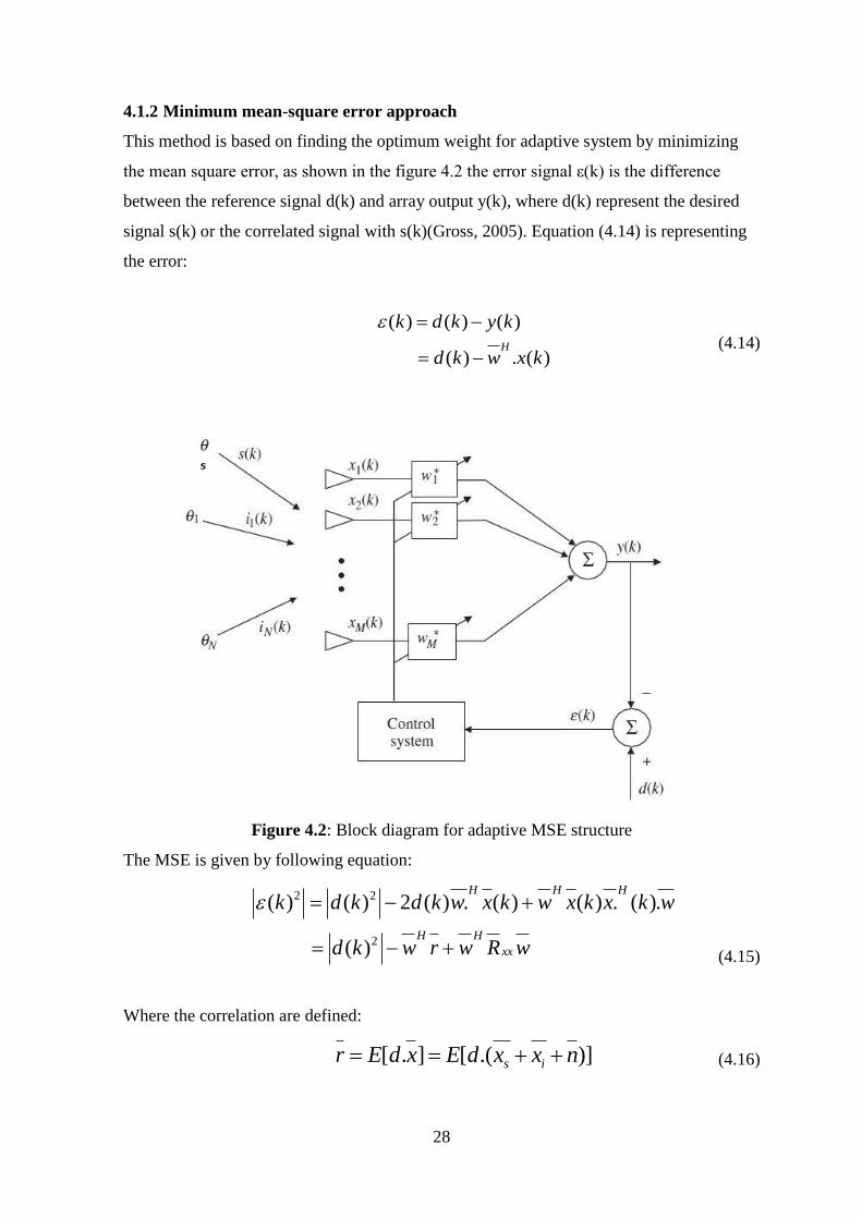
This method is based on finding the optimum weight for adaptive system by minimizing
the mean square error, as shown in the figure 4.2 the error signal ε(k) is the difference
between the reference signal d(k) and array output y(k), where d(k) represent the desired
signal s(k) or the correlated signal with s(k)(Gross, 2005). Equation (4.14) is representing
the error:
( ) ( ) ( )
( ) . ( )H
k d k y k
d k w x k
(4.14)
Figure 4.2: Block diagram for adaptive MSE structure
The MSE is given by following equation:
2 2
2
( ) ( ) 2 ( ) . ( ) ( ) . ( ).
( )
H H H
H H
xx
k d k d k w x k w x k x k w
d k w r w R w
(4.15)
Where the correlation are defined:
[ . ] [ .( )]s ir E d x E d x x n (4.16)
29
[ ]H
xx SS uuR E xx R R (4.17)
While ssR and
uuR have been defined in equations (4.7) and (4.8).
By using algebraic operations with Wiener-Hopf equation (4.19), it becomes possible to
obtain the optimum weight which is the minimum MSE, thus the solution given as in the
following equation:
2( [ ( ) ]) 2 2 0xx
wE k R w r (4.18)
1
xxMSEw R r
(4.19)
4.1.3 Maximum likelihood approach
In this method the target is to estimate the desired signal, where ML method is based on
the assumption that the desired signal sx is unknown and there is no feedback to array
elements while the unwanted signal n has a zero mean Gaussian distribution (Gross,
2005).The input signal vector is given by:
sx x n (4.20)
The probability function is given by:
1(( ) ( ))
2
1( )
2
Hnns sx x R x x
s
n
p x x e
(4.21)
Where the noise standard deviation referred to as n and Rnn is correlation matrix of the
noise signal, the log-likelihood expression can be defined as :
1
[ ] ln[ ( )] ( ) ( )Hnns s sL x p x x C x x R x x
(4.22)
By Taking the partial derivative of [ ]L x with respect to s and setting it equal to zero in
order to find the maximum of L ,After doing some calculations we can get the optimum
weight Where is expressed as follows:
1
1
nn sML H
SSs s
R aw
a R a
(4.23)
30
4.1.4 Minimum Variance approach
This method is similar to the Maximum Likelihood solution, but the MV is more general
than ML in its application, where minimum variance method can contain interferences
signals and noise as unwanted signals within the input signal. However, all unwanted
signals in ML methods are zero mean with Gaussian distribution.
The main target of minimum variance approach is to decrease the noise variance of the
output array, thus it is supposed that the unwanted and desired signals have zero mean
(Gross, 2005).
The output array with respective weight is expressed as:
H H H
sy w x w a s w u (4.24)
For distortion-less response, the constraint is H
sw a = 1, and after applying this constraint
to equation (4.25) the output array will given as:
H
y s w u (4.25)
In order to find the variance of array output we can write:
2 22 [ ] [ ]
H H
MV
H
uu
E w x E s w u
w R w
(4.26)
The Lagrange Method that is used in order to minimize the convergence depends on the
cost function which is defined as:
2
( ) (1 )2
(1 )2
HMV
s
HHuu
s
J w w a
w R ww a
(4.27)
Where Lagrange multiplier λ is:
1
1
s suua R a
(4.28)
In order to find the minimum variance weight, the cost function must be minimize by
setting gradient equal to zero such as:
1MV suuw R a (4.29)
After substituting equation(4.29) into equation. (4.30), the optimum minimum variance
weight is:
31
1
1MV
suu
s suu
R aw
a R a
(4.30)
4.2 Adaptive Beam forming
The term adaptive refers to the capability to update and adjust the weights continuously
with the changing angles of arrived signals with time, while previous methods find the
optimal weight without having to the re-calculations and that because the angles of arrived
signals remain constant and do not change with the times(Gross, 2005).
In order to maximize the output signal power in desired direction and minimize the power
in the unwanted direction, various powerful algorithms are used to adjust the weights of
the smart antenna array adaptively, so that the output beam pattern is optimized for
enhancing the system (RAO & SARMA, 2014). There are numerous algorithms used in
beamformer optimization for the sake of reduction of interferences, side-lobes and noise
such as lest mean square algorithm (LMS),recursive lest square (RLS), Sample matrix
inversion algorithm (SMI) and the constant modulus algorithm (CMA).
In reception part of smart antenna system, the beam former implements the signal data of
the training to establish the optimal vector of weights during the training time, data is then
passed and the beam former investigates the computed weight vector to analyse any
received signal. However, beamforming algorithms is classified as Blind algorithms and
Non blind algorithms, where the first category (Blind Algorithm) doesn’t use the desired
signal d(t) a while the second category (Non blind algorithm)use the desired signal d(t)
which is based on a knowledge of the nature of the received signals as a training signal in
training period. (Mallaparapu, et al., 2011).In the following sections we will discuss the
most popular optimization algorithms.
4.2.1 Least mean square algorithm (LMS)
LMS algorithm was created by Wirodw and Hoff in 1960 (Haykin, 2002). This method is
classified as a non-blind adaptive algorithm because it requires training sequence.
By gradient method this algorithm can adjust the weights based on MSE(Minimum square
Error) which is calculated from the difference between the input signal and desired signal,
this ability to update the weights is based on the availability of information about desired
signal and input vector, furthermore it doesn’t need to correlation function or matrix
32
inversion computation that makes this method simple and a reasonable choice for many
application in ASP(Rahaman, Hossain, & Rana, 2013).
The output signal y(n) is the weighted sum of the input signals x(n), where these input
signals are multiplied by the input complex weights W, and they are expressed in
following equation: where x is the received input vector
y(K)=w ( ). ( )H K x K (4.31)
Where x is the received input vector Where and wT is the transpose of the weight vector
w [ (1) (2) (3).... ( )]T Tw w w w n .
The error signal is considered as a control signals in weights adaptation process and is
defined as:
( ) ( ) ( )
( ) w . ( )H
e K d K y K
d K x K
(4.32)
However, this algorithms aims to make the output response for each element equal or close
to the desired response in each iteration until all weights converge (Hreshee D. S., 2013),
this weight adaptation method is done by this equation :
( 1) ( ) ( ) ( )w K w K e K x K (4.33)
Where is step size which controls the convergence of algorithms and the adaptation rate
(Ramineni, Sagar, K.Abhishek Jain, T.V.Ramakrishna, & Kumar, 2012),this parameter is
restricted is restricted as follows:
max
10
(4.34)
So that if the convergence of algorithm will be fast if is chosen to be large, while the
convergence becomes slow if is small. Moreover, the step size is depends on max which
is largest Eigen value of autocorrelation matrix Ruu (Rahaman, Hossain, & Rana, 2013).
4.2.2 Recursive least square algorithm (RLS)
RLS is one of the most popular adaptive beam-forming algorithms based on recursive least
square. This algorithm requires no matrix inversion because correlation matrix is found
directly. It uses the sum of squared errors for the inputs to update the complex weights instead
of using the mean square error minimization. The first adaptation of this algorithm was derived
33
from KALMAN filter for multi tap transversal filtering where samples are taken over variable
time frame. However, this algorithm is applicable for other systems where the inputs are
extracted from different sources. The algorithm uses desired signal and correlation matrix in
the adaptation. The following equation is used to update the weight values.
( ) ( 1) ( )[ ( ) ( ) ( 1)]w k w k g k d k x k w k (4.35)
In order to solve the slow convergence speed in LMS algorithm, step size parameter is
replaced by the gain vector ( )g k which is defined as (Rani, Subbaiah, Reddy, & Rani, 2009):
1
( ) ( )xxg k R x k
(4.36)
And xxR
is the correlation matrix expressed as:
1
( ) ( )K
H
xx
i
R x i x i
(4.37)
4.2.3 Constant-modulus (CM) algorithm
The Constant Modulus algorithm is called as blind algorithm because the desired signal is not
available. The algorithm is performed through the use of three distinct steps in each turn. In the
first step, the computation of the processed signal with the actual weights is performed. In the
second step, an error is generated from the computed signal. Finally, the weights are adapted
with new error data in the third step. The algorithm can be expressed mathematically in the
following equations.
The error signal is calculated without resorting to the reference signal, this error is given
by:
2
( ) ( ) ( ) ( ( ) )p p
Pe k y k y k R y k
(4.38)
Where the weighted output y(k) is given as:
y(K)=w . ( )H x K (4.39)
The Godard cost function is expressed as:
( ) [( ( ) ) ]p q
PJ K E y k R (4.40)
When the gradient of cost function is zero, then the is expressed as:
2[ ( ) ]
[ ( ) ]
P
P P
E s kR
E s k (4.41)

34
Where q is a positive integer=1, p is positive integer, and s(k) is the zero-memory estimate
of y(k). In this algorithm the weights are updated by following equation:
( 1) ( ) ( ) ( )w K w K e K x K (4.42)
35
CHAPTER 5
ARTIFICIAL NEURAL NETWORKS (ANN) AND OPTIMAZATION OF
ANTENNA ARRAY
Artificial neural networks (ANNs) are considered the artificial equivalent in function and
construction of the real human brain. Human brain is a very complex and interconnected
network of neural cells; this complex structure is capable to accomplish hard and complex
tasks in an easy way that can’t be imagined. This structure gives the brain a very important
sense of creativity in the way it does the different tasks. Mathematic operations, logical
thinking, decision making, and many other tasks are examples of the non linear tasks that
brain can do in a soft manner. One important characteristic of the human brain and the
neural system is its ability to learn things and to create things that didn’t exist based on
experience.
Scientists started studying the structure of the human brain early; however, the real steps
toward imitating the structure of biological neural structure started in the 5th
decade of the
20th
century. McCulloch and Pitts have introduced the simplest structure of neurons in
1943 and presented it as models of real neurons. They were claimed to be the basic
structure of the computational circuits of the future that exactly works like human brains
do (Krose & Smagt, 1996). During the 1950s, real implementation of artificial neural
networks started to be presented (Fyfe, 1996). In our days, artificial neural networks have
become very famous and well known in the world of science. Many sciences use artificial
neural networks in very advanced tasks. Artificial neural networks are mostly implemented
in medical applications and image processing (Khashman, Automatic Edge Detection of
DNA Bands in Autoradiograph Images, 1999) (Khashman & Dimililer, 2007). Artificial
neural network are also used in control systems and procedures, prediction and prices
estimation, communication systems, and weather forecasting. Artificial neural networks
can also be used in the field of communication and more precisely in smart antenna
applications (Hreshee S. , 2013) (merad, Bendimerad, & Sidi Mohamed Meriah, 2007)
(Saleh, AL-Ali, & Alssarn, 2013).
The use of artificial neural network in any task implies starting by teaching the networks
by updating the values of its neurons based on past experience or examples. The well
known back propagation algorithm is one of the most powerful learning algorithms of
artificial neural networks. This algorithm was firstly proposed in 1969 by Yu-Chi Ho and
others; it was applied in ANN applications on 1974 by Rumelhart, Werbos, and others.
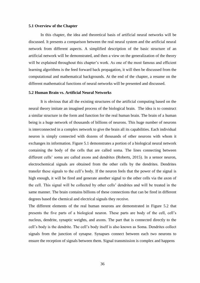
36
5.1 Overview of the Chapter
In this chapter, the idea and theoretical basis of artificial neural networks will be
discussed. It presents a comparison between the real neural system and the artificial neural
network from different aspects. A simplified description of the basic structure of an
artificial network will be demonstrated, and then a view on the generalization of the theory
will be explained throughout this chapter’s work. As one of the most famous and efficient
learning algorithms is the feed forward back propagation, it will then be discussed from the
computational and mathematical backgrounds. At the end of the chapter, a resume on the
different mathematical functions of neural networks will be presented and discussed.
5.2 Human Brain vs. Artificial Neural Networks
It is obvious that all the existing structures of the artificial computing based on the
neural theory imitate an imagined process of the biological brain. The idea is to construct
a similar structure in the form and function for the real human brain. The brain of a human
being is a huge network of thousands of billions of neurons. This huge number of neurons
is interconnected in a complex network to give the brain all its capabilities. Each individual
neuron is simply connected with dozens of thousands of other neurons with whom it
exchanges its information. Figure 5.1 demonstrates a portion of a biological neural network
containing the body of the cells that are called soma. The lines connecting between
different cells’ soma are called axons and dendrites (Roberts, 2015). In a sensor neuron,
electrochemical signals are obtained from the other cells by the dendrites. Dendrites
transfer these signals to the cell’s body. If the neuron feels that the power of the signal is
high enough, it will be fired and generate another signal to the other cells via the axon of
the cell. This signal will be collected by other cells’ dendrites and will be treated in the
same manner. The brain contains billions of these connections that can be fired in different
degrees based the chemical and electrical signals they receive.
The different elements of the real human neurons are demonstrated in Figure 5.2 that
presents the five parts of a biological neuron. These parts are body of the cell, cell’s
nucleus, dendrite, synaptic weights, and axons. The part that is connected directly to the
cell’s body is the dendrite. The cell’s body itself is also known as Soma. Dendrites collect
signals from the junction of synapse. Synapses connect between each two neurons to
ensure the reception of signals between them. Signal transmission is complex and happens
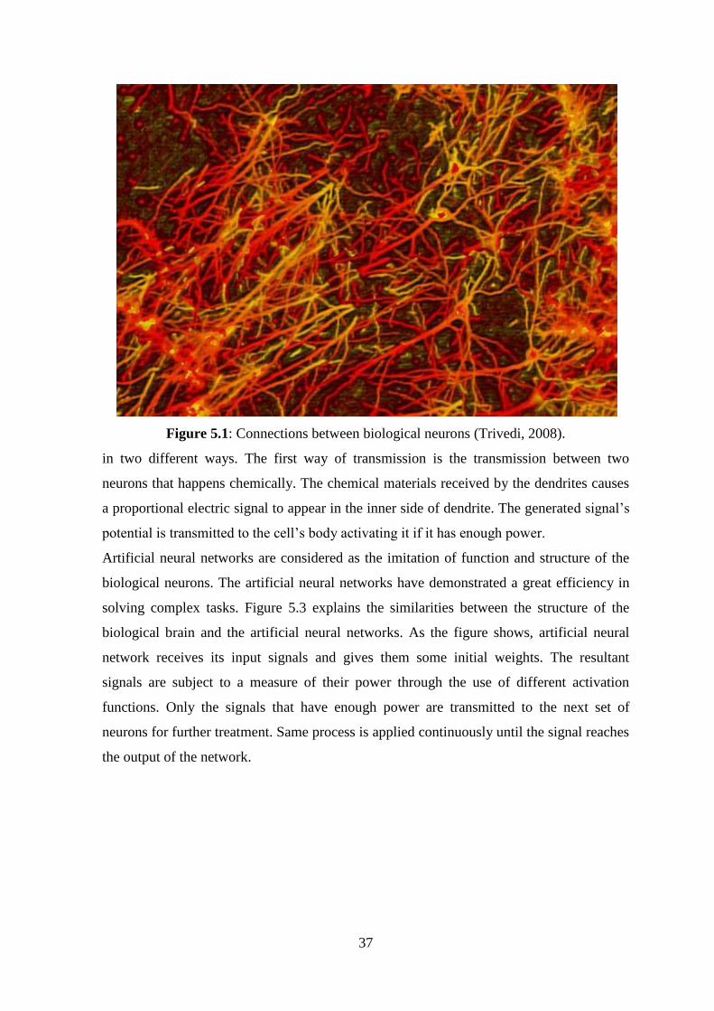
37
Figure 5.1: Connections between biological neurons (Trivedi, 2008).
in two different ways. The first way of transmission is the transmission between two
neurons that happens chemically. The chemical materials received by the dendrites causes
a proportional electric signal to appear in the inner side of dendrite. The generated signal’s
potential is transmitted to the cell’s body activating it if it has enough power.
Artificial neural networks are considered as the imitation of function and structure of the
biological neurons. The artificial neural networks have demonstrated a great efficiency in
solving complex tasks. Figure 5.3 explains the similarities between the structure of the
biological brain and the artificial neural networks. As the figure shows, artificial neural
network receives its input signals and gives them some initial weights. The resultant
signals are subject to a measure of their power through the use of different activation
functions. Only the signals that have enough power are transmitted to the next set of
neurons for further treatment. Same process is applied continuously until the signal reaches
the output of the network.

38
Figure 5.2: Elements of biological neuron (Sadhu, 2012).
Input Layer Hidden layers Output
layer
Inp
ut
Ou
tpu
t
Vs.
Artificial networksBiological networks
Figure 5.3: Analogy between human brain and neural networks
5.3 Artificial Neural Networks
Artificial neural networks are very powerful structures of computation units that
were stimulated from the brain model. They were constructed to help solving non linear
complex problems where normal mathematical approaches seem inefficient. The main
similarity between a biological and artificial thinking structure is the need for learning. The
same way in which biological neurons work, artificial neurons can accomplish their
required tasks. Each single neuron’s signal worth to be transmitted if it receives signals
with enough power to activate its output from the previous neurons; otherwise, the output
from the neuron will not be generated and transmitted to the next neuron. In some cases,
39
the power of an output signal generated by a neuron is proportional to the sum of its input
signals. Figure 5.4 reveals the idea of power of signal and activation of the output signal.
The input signals are given some arbitrary weights based on previous knowledge or
training. The power of the neurons signal is measured by summing all received signals
with respect to their weights. The total power is presented to the activation or transfer
function to determine an appropriate output power. The total power received by a neuron
can be expressed by:
1
*N
n n
n
S I
(5.1)
Generated
signal ∑
1I1
2I2
nIn
NIN
Transfer
function
Signal
Power
Figure 5.4: Construction of artificial neural network.
5.4 Basic Elements of Artificial Network
Any artificial network needs mainly three features and training algorithm to be able
to perform a required task. These features are mainly the weights, transfer functions, and
layers. These are the three main functional parts of an artificial neural structure. The
learning method is the algorithm used to adapt the neural network to do the required task.
5.4.1 ANN layers
Layers are one of the important parts of any artificial neural network’s structure.
Connections between successive layers give the neural network its main functionality. Data
is processed through different layers from one layer to another. Each layer receives some
data from the previous layers, process this data, and transfer it to the next layer. Layers are
divided into three different categories, input layers where input data is received from the
systems, output layer where output results are displayed or submitted to other systems, and
between these two layers one or more hidden layers ensures the flow of these data.
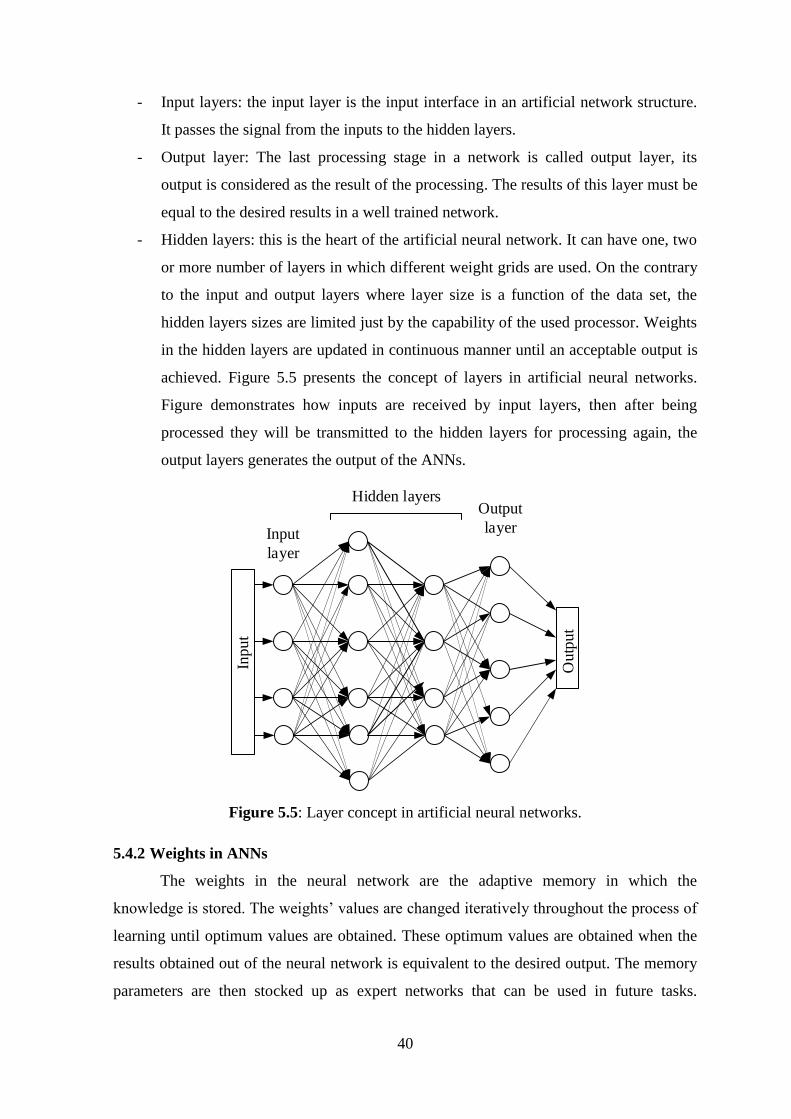
40
- Input layers: the input layer is the input interface in an artificial network structure.
It passes the signal from the inputs to the hidden layers.
- Output layer: The last processing stage in a network is called output layer, its
output is considered as the result of the processing. The results of this layer must be
equal to the desired results in a well trained network.
- Hidden layers: this is the heart of the artificial neural network. It can have one, two
or more number of layers in which different weight grids are used. On the contrary
to the input and output layers where layer size is a function of the data set, the
hidden layers sizes are limited just by the capability of the used processor. Weights
in the hidden layers are updated in continuous manner until an acceptable output is
achieved. Figure 5.5 presents the concept of layers in artificial neural networks.
Figure demonstrates how inputs are received by input layers, then after being
processed they will be transmitted to the hidden layers for processing again, the
output layers generates the output of the ANNs.
Input
layer
Output
layer
Outp
ut
Inpu
t
Hidden layers
Figure 5.5: Layer concept in artificial neural networks.
5.4.2 Weights in ANNs
The weights in the neural network are the adaptive memory in which the
knowledge is stored. The weights’ values are changed iteratively throughout the process of
learning until optimum values are obtained. These optimum values are obtained when the
results obtained out of the neural network is equivalent to the desired output. The memory
parameters are then stocked up as expert networks that can be used in future tasks.
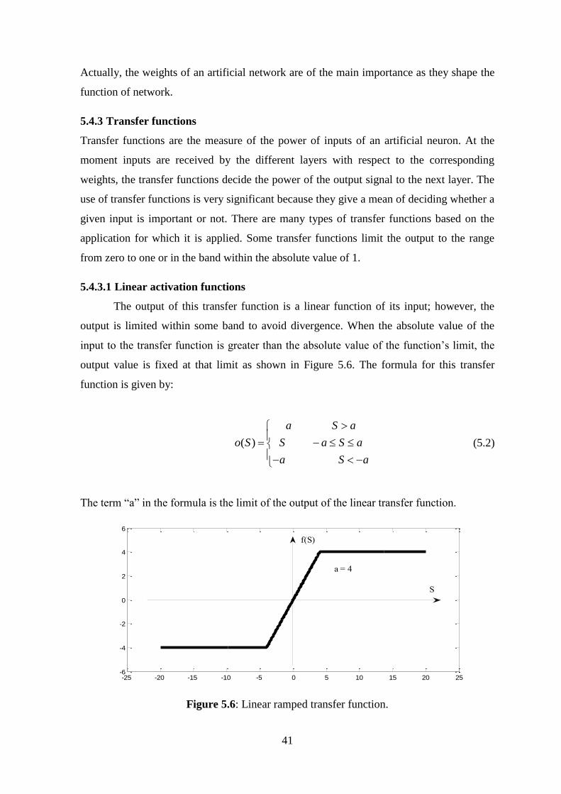
41
Actually, the weights of an artificial network are of the main importance as they shape the
function of network.
5.4.3 Transfer functions
Transfer functions are the measure of the power of inputs of an artificial neuron. At the
moment inputs are received by the different layers with respect to the corresponding
weights, the transfer functions decide the power of the output signal to the next layer. The
use of transfer functions is very significant because they give a mean of deciding whether a
given input is important or not. There are many types of transfer functions based on the
application for which it is applied. Some transfer functions limit the output to the range
from zero to one or in the band within the absolute value of 1.
5.4.3.1 Linear activation functions
The output of this transfer function is a linear function of its input; however, the
output is limited within some band to avoid divergence. When the absolute value of the
input to the transfer function is greater than the absolute value of the function’s limit, the
output value is fixed at that limit as shown in Figure 5.6. The formula for this transfer
function is given by:
( )
a S a
o S S a S a
a S a
(5.2)
The term “a” in the formula is the limit of the output of the linear transfer function.
Figure 5.6: Linear ramped transfer function.
-25 -20 -15 -10 -5 0 5 10 15 20 25-6
-4
-2
0
2
4
6
S
a = 4
f(S)
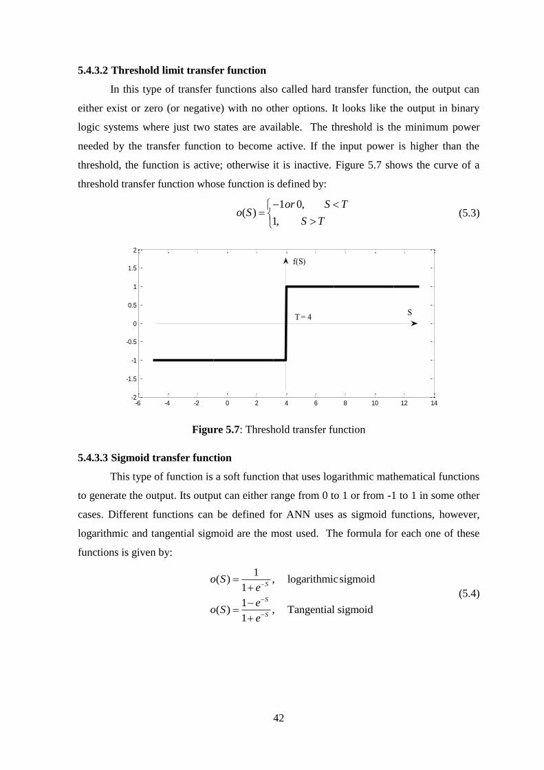
42
5.4.3.2 Threshold limit transfer function
In this type of transfer functions also called hard transfer function, the output can
either exist or zero (or negative) with no other options. It looks like the output in binary
logic systems where just two states are available. The threshold is the minimum power
needed by the transfer function to become active. If the input power is higher than the
threshold, the function is active; otherwise it is inactive. Figure 5.7 shows the curve of a
threshold transfer function whose function is defined by:
1 0,
( )1,
or S To S
S T
(5.3)
Figure 5.7: Threshold transfer function
5.4.3.3 Sigmoid transfer function
This type of function is a soft function that uses logarithmic mathematical functions
to generate the output. Its output can either range from 0 to 1 or from -1 to 1 in some other
cases. Different functions can be defined for ANN uses as sigmoid functions, however,
logarithmic and tangential sigmoid are the most used. The formula for each one of these
functions is given by:
1( ) , logarithmicsigmoid
1
1( ) , Tangential sigmoid
1
S
S
S
o Se
eo S
e
(5.4)
-6 -4 -2 0 2 4 6 8 10 12 14-2
-1.5
-1
-0.5
0
0.5
1
1.5
2
S
f(S)
T = 4
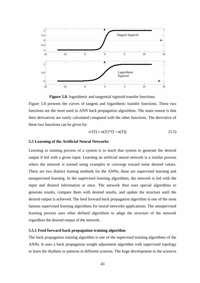
43
Figure 5.8: logarithmic and tangential sigmoid transfer functions.
Figure 5.8 presents the curves of tangent and logarithmic transfer functions. These two
functions are the most used in ANN back propagation algorithms. The main reason is that
their derivatives are easily calculated compared with the other functions. The derivative of
these two functions can be given by:
'( ) ( )*(1 ( ))o S o S o S (5.5)
5.5 Learning of the Artificial Neural Networks
Learning or training process of a system is to teach that system to generate the desired
output if fed with a given input. Learning an artificial neural network is a similar process
where the network is trained using examples to converge toward some desired values.
There are two distinct leaning methods for the ANNs; these are supervised learning and
unsupervised learning. In the supervised learning algorithms, the network is fed with the
input and desired information at once. The network then uses special algorithms to
generate results, compare them with desired results, and update the structure until the
desired output is achieved. The feed forward back propagation algorithm is one of the most
famous supervised learning algorithms for neural networks applications. The unsupervised
learning process uses other defined algorithms to adapt the structure of the network
regardless the desired output of the network.
5.5.1 Feed forward back propagation training algorithm
The back propagation training algorithm is one of the supervised training algorithms of the
ANNs. It uses a back propagation weight adjustment algorithm with supervised topology
to learn the rhythms or patterns in different systems. The huge development in the sciences
-15 -10 -5 0 5 10 15
-1
-0.5
0
0.5
1
-15 -10 -5 0 5 10 15
0
0.5
1
LagarithmicSigmoid
Tangent Sigmoid
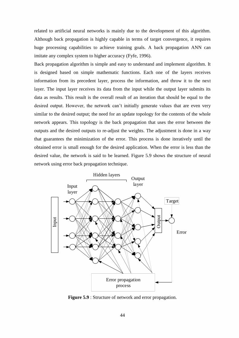
44
related to artificial neural networks is mainly due to the development of this algorithm.
Although back propagation is highly capable in terms of target convergence, it requires
huge processing capabilities to achieve training goals. A back propagation ANN can
imitate any complex system to higher accuracy (Fyfe, 1996).
Back propagation algorithm is simple and easy to understand and implement algorithm. It
is designed based on simple mathematic functions. Each one of the layers receives
information from its precedent layer, process the information, and throw it to the next
layer. The input layer receives its data from the input while the output layer submits its
data as results. This result is the overall result of an iteration that should be equal to the
desired output. However, the network can’t initially generate values that are even very
similar to the desired output; the need for an update topology for the contents of the whole
network appears. This topology is the back propagation that uses the error between the
outputs and the desired outputs to re-adjust the weights. The adjustment is done in a way
that guarantees the minimization of the error. This process is done iteratively until the
obtained error is small enough for the desired application. When the error is less than the
desired value, the network is said to be learned. Figure 5.9 shows the structure of neural
network using error back propagation technique.
Input
layer
Output
layer
Error
Outp
ut
Target
Error propagation
process
Inpu
t
Hidden layers
Figure 5.9 : Structure of network and error propagation.
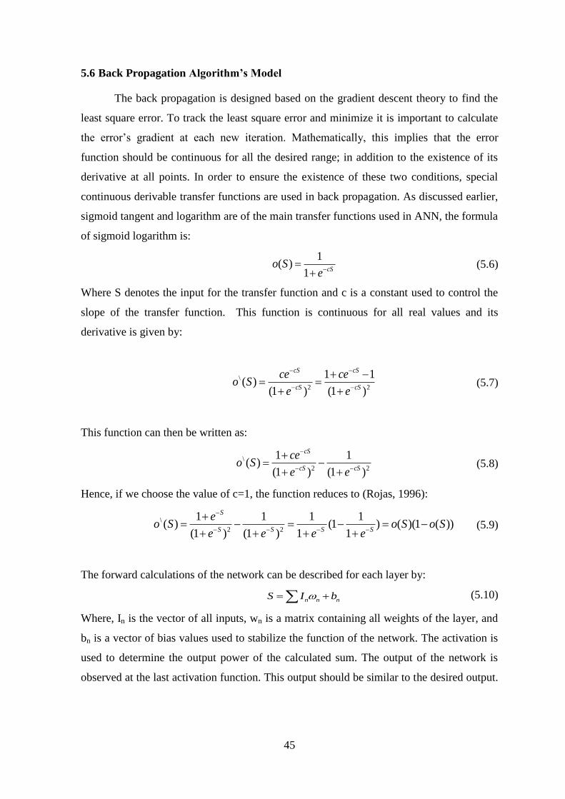
45
5.6 Back Propagation Algorithm’s Model
The back propagation is designed based on the gradient descent theory to find the
least square error. To track the least square error and minimize it is important to calculate
the error’s gradient at each new iteration. Mathematically, this implies that the error
function should be continuous for all the desired range; in addition to the existence of its
derivative at all points. In order to ensure the existence of these two conditions, special
continuous derivable transfer functions are used in back propagation. As discussed earlier,
sigmoid tangent and logarithm are of the main transfer functions used in ANN, the formula
of sigmoid logarithm is:
1
( )1 cS
o Se
(5.6)
Where S denotes the input for the transfer function and c is a constant used to control the
slope of the transfer function. This function is continuous for all real values and its
derivative is given by:
\
2 2
1 1( )
(1 ) (1 )
cS cS
cS cS
ce ceo S
e e
(5.7)
This function can then be written as:
\
2 2
1 1( )
(1 ) (1 )
cS
cS cS
ceo S
e e
(5.8)
Hence, if we choose the value of c=1, the function reduces to (Rojas, 1996):
\
2 2
1 1 1 1( ) (1 ) ( )(1 ( ))
(1 ) (1 ) 1 1
S
S S S S
eo S o S o S
e e e e
(5.9)
The forward calculations of the network can be described for each layer by:
n n nS I b (5.10)
Where, In is the vector of all inputs, wn is a matrix containing all weights of the layer, and
bn is a vector of bias values used to stabilize the function of the network. The activation is
used to determine the output power of the calculated sum. The output of the network is
observed at the last activation function. This output should be similar to the desired output.
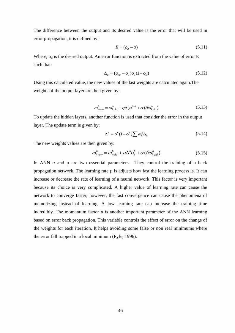
46
The difference between the output and its desired value is the error that will be used in
error propagation, it is defined by:
( )dE o o (5.11)
Where, od is the desired output. An error function is extracted from the value of error E
such that:
( ) (1 )k dk k k ko o o o (5.12)
Using this calculated value, the new values of the last weights are calculated again.The
weights of the output layer are then given by:
1 ( )h h h h h
k new k old k k oldo (5.13)
To update the hidden layers, another function is used that consider the error in the output
layer. The update term is given by:
(1 )h h h h
k ko o (5.14)
The new weights values are then given by:
( )h h h h h
k new k old k k oldo (5.15)
In ANN α and µ are two essential parameters. They control the training of a back
propagation network. The learning rate µ is adjusts how fast the learning process is. It can
increase or decrease the rate of learning of a neural network. This factor is very important
because its choice is very complicated. A higher value of learning rate can cause the
network to converge faster; however, the fast convergence can cause the phenomena of
memorizing instead of learning. A low learning rate can increase the training time
incredibly. The momentum factor α is another important parameter of the ANN learning
based on error back propagation. This variable controls the effect of error on the change of
the weights for each iteration. It helps avoiding some false or non real minimums where
the error fall trapped in a local minimum (Fyfe, 1996).
47
CHAPTER 6
SIMULATION AND RESULT FOR UNIFORM LINEAR ARRAY
This chapter presents simulation for ULA antenna array by using MATLAB. This
simulation process analyses and compare the performance of popular adaptive techniques
such as LMS, RLS and CMA. The comparison considered different criterions including
amplitude response, convergence time, acquisition and tracking of desired signal .The
parameters that were used during the simulation are:
Table 6.1: Parameters of the desired and interference AOA
DOA of desired signal 30˚
DOA of interference signal
-60˚
6.1 Comparison of Amplitude Responses of LMS, RLS and CMA Algorithms
In this part, simulation was carried out for the same algorithm with different antenna array
parameters such as number of sensor elements and distance between each two elements in
the antenna array. The simulation results for various numbers of elements and different
distances between successive elements are shown in the next figures. 5, 8, and 10 elements
arrays were used at distances of d=0.125λ, 0.25λ, and 0.5λ were carried out. The maximum
distance between two elements was restricted to 0.5λ to avoid spatial aliasing.
6.1.1 LMS algorithm
FIGURE 6.1 presents the amplitude response of the Least Mean Square algorithm for
different number of elements of array at distance d=0.5λ. It is obvious that using LMS
algorithm the response has given amplitude of one at the desired angle and cancelled
totally the unwanted signal. The use of 10 elements in the array has ameliorated the
response of the algorithm by narrowing the band of the response. Figure 6.2 shows the
same results for the case of using d=0.25 and d=0.125λ. The obtained results show that the
higher the number of array elements the better the response of the algorithm. However, the
response accuracy decreases with the decrease of the distance between elements of the
array. As seen from Figure 6.2 to the left, the passing band is wider than the case of 0.5λ.
This band becomes wider in the case of 0.125λ as in Figure 6.2 to the right.
48
Figure 6.1: Array Factor plots for LMS algorithm (d=0.5λ)
Figure 6.2: Array Factor plots for LMS algorithm
6.1.2 RLS algorithm
In this part, the same experiments were applied by using the RLS algorithm. The results
are shown in Figure , Figure 6., and Figure . The results show that the response is better
when using higher number of elemnts. The response is showing amplitude of
approximately 0.4 at some undesired angles of arrival. Such values are considered as
drwbacks of the algorithm. The results of N=10 were better in the case of d=0.5λ; however,
this was not the case when using d=0.25λ and d=0.125λ. the case of N=8 has given better
performance. The performance in term of passing band has shown better performance for
smaller inter-element distance.
-90 -60 -30 0 30 60 900
0.2
0.4
0.6
0.8
1
AOA (deg)
|AF
n|
d =0.5
N=5
N=8
N=10
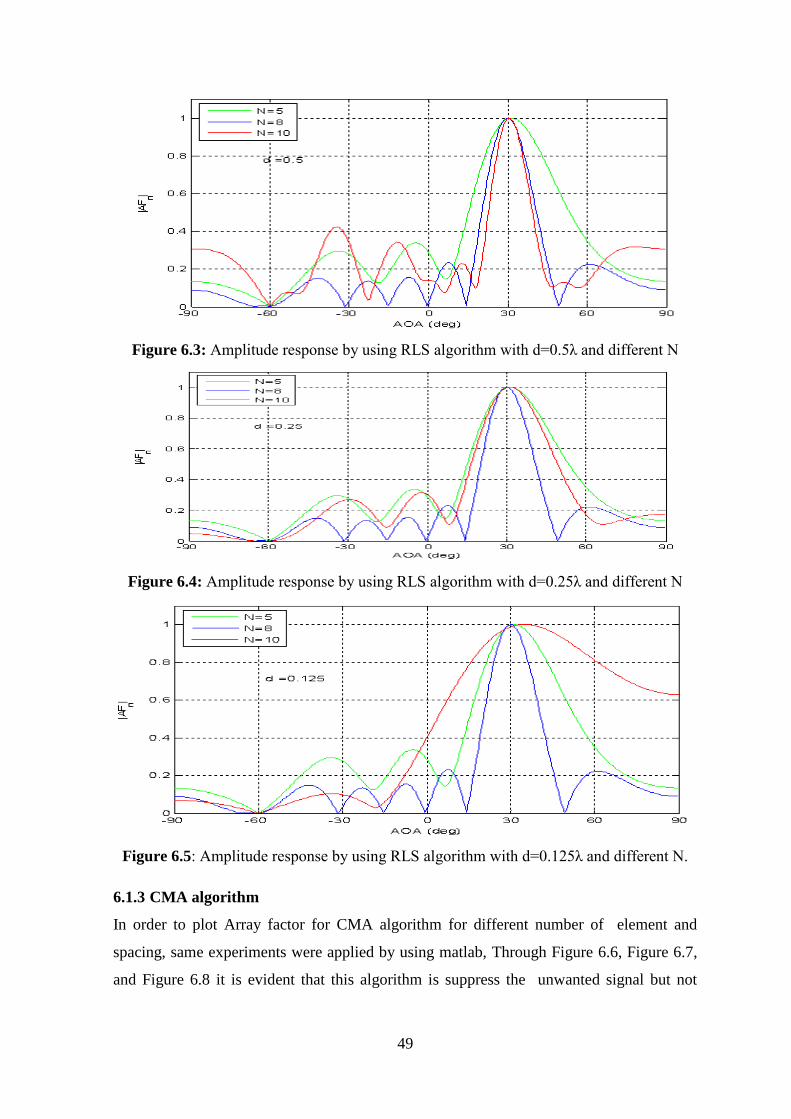
49
Figure 6.3: Amplitude response by using RLS algorithm with d=0.5λ and different N
Figure 6.4: Amplitude response by using RLS algorithm with d=0.25λ and different N
Figure 6.5: Amplitude response by using RLS algorithm with d=0.125λ and different N.
6.1.3 CMA algorithm
In order to plot Array factor for CMA algorithm for different number of element and
spacing, same experiments were applied by using matlab, Through Figure 6.6, Figure 6.7,
and Figure 6.8 it is evident that this algorithm is suppress the unwanted signal but not
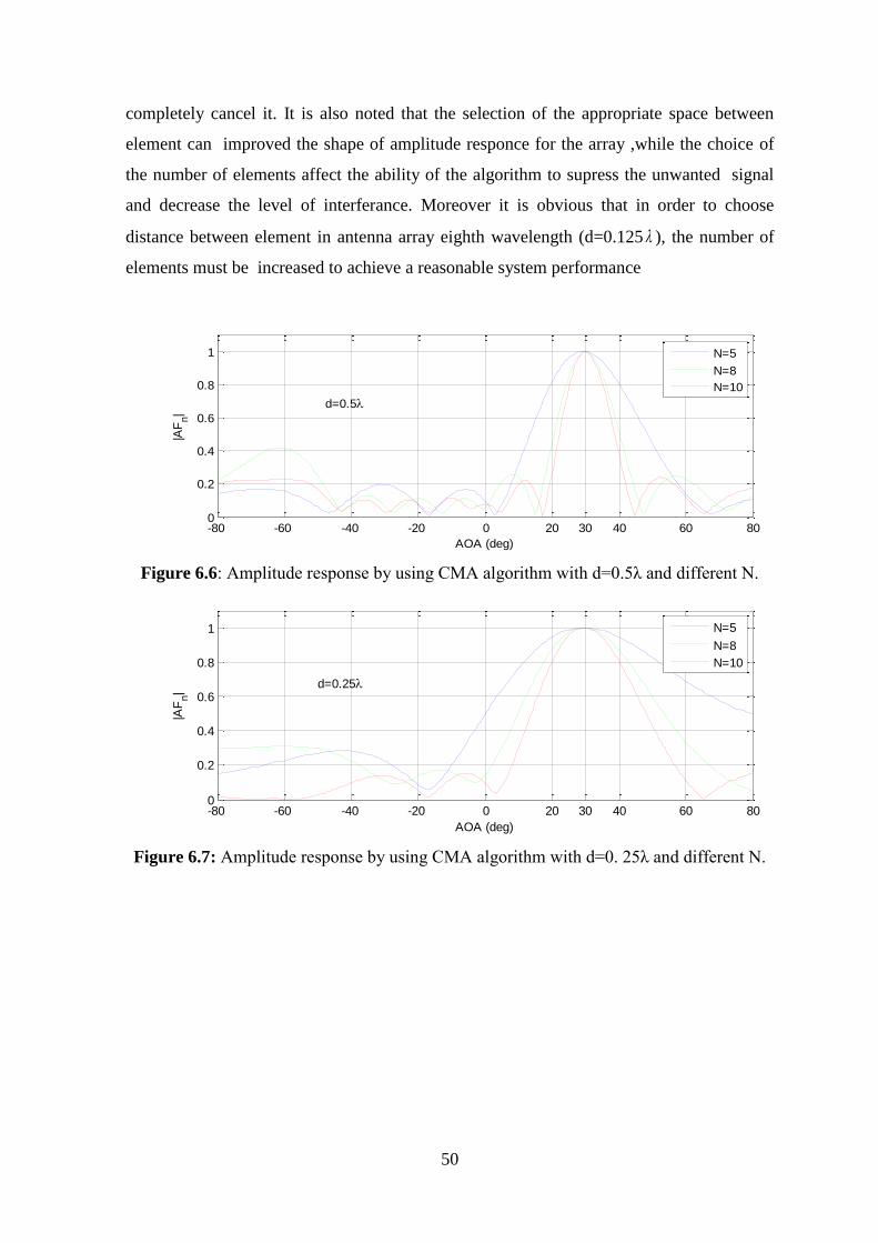
50
completely cancel it. It is also noted that the selection of the appropriate space between
element can improved the shape of amplitude responce for the array ,while the choice of
the number of elements affect the ability of the algorithm to supress the unwanted signal
and decrease the level of interferance. Moreover it is obvious that in order to choose
distance between element in antenna array eighth wavelength (d=0.125 ), the number of
elements must be increased to achieve a reasonable system performance
Figure 6.6: Amplitude response by using CMA algorithm with d=0.5λ and different N.
Figure 6.7: Amplitude response by using CMA algorithm with d=0. 25λ and different N.
-80 -60 -40 -20 0 3020 40 60 800
0.2
0.4
0.6
0.8
1
AOA (deg)
|AF
n|
d=0.5
N=5
N=8
N=10
-80 -60 -40 -20 0 3020 40 60 800
0.2
0.4
0.6
0.8
1
AOA (deg)
|AF
n|
d=0.25
N=5
N=8
N=10
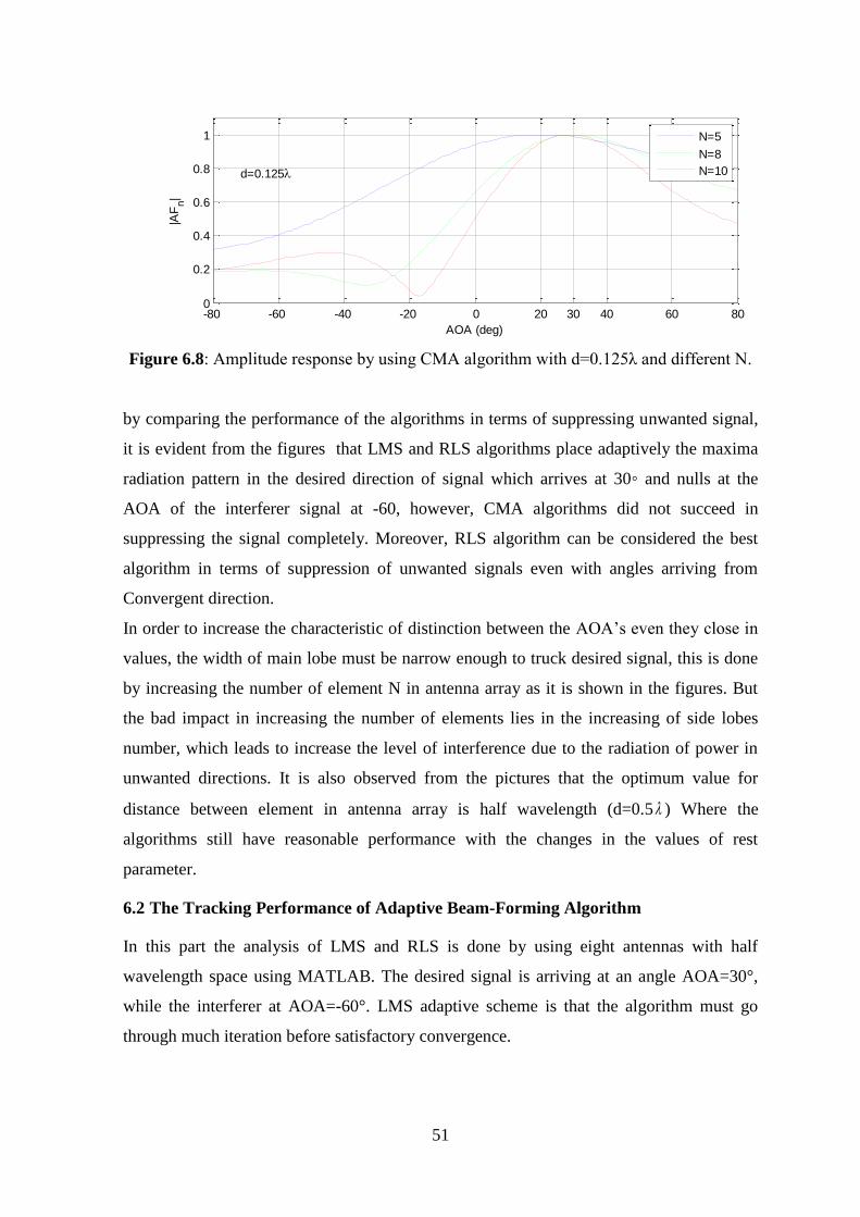
51
Figure 6.8: Amplitude response by using CMA algorithm with d=0.125λ and different N.
by comparing the performance of the algorithms in terms of suppressing unwanted signal,
it is evident from the figures that LMS and RLS algorithms place adaptively the maxima
radiation pattern in the desired direction of signal which arrives at 30◦ and nulls at the
AOA of the interferer signal at -60, however, CMA algorithms did not succeed in
suppressing the signal completely. Moreover, RLS algorithm can be considered the best
algorithm in terms of suppression of unwanted signals even with angles arriving from
Convergent direction.
In order to increase the characteristic of distinction between the AOA’s even they close in
values, the width of main lobe must be narrow enough to truck desired signal, this is done
by increasing the number of element N in antenna array as it is shown in the figures. But
the bad impact in increasing the number of elements lies in the increasing of side lobes
number, which leads to increase the level of interference due to the radiation of power in
unwanted directions. It is also observed from the pictures that the optimum value for
distance between element in antenna array is half wavelength (d=0.5 ) Where the
algorithms still have reasonable performance with the changes in the values of rest
parameter.
6.2 The Tracking Performance of Adaptive Beam-Forming Algorithm
In this part the analysis of LMS and RLS is done by using eight antennas with half
wavelength space using MATLAB. The desired signal is arriving at an angle AOA=30°,
while the interferer at AOA=-60°. LMS adaptive scheme is that the algorithm must go
through much iteration before satisfactory convergence.
-80 -60 -40 -20 0 3020 40 60 800
0.2
0.4
0.6
0.8
1
AOA (deg)
|AF
n|
d=0.125
N=5
N=8
N=10
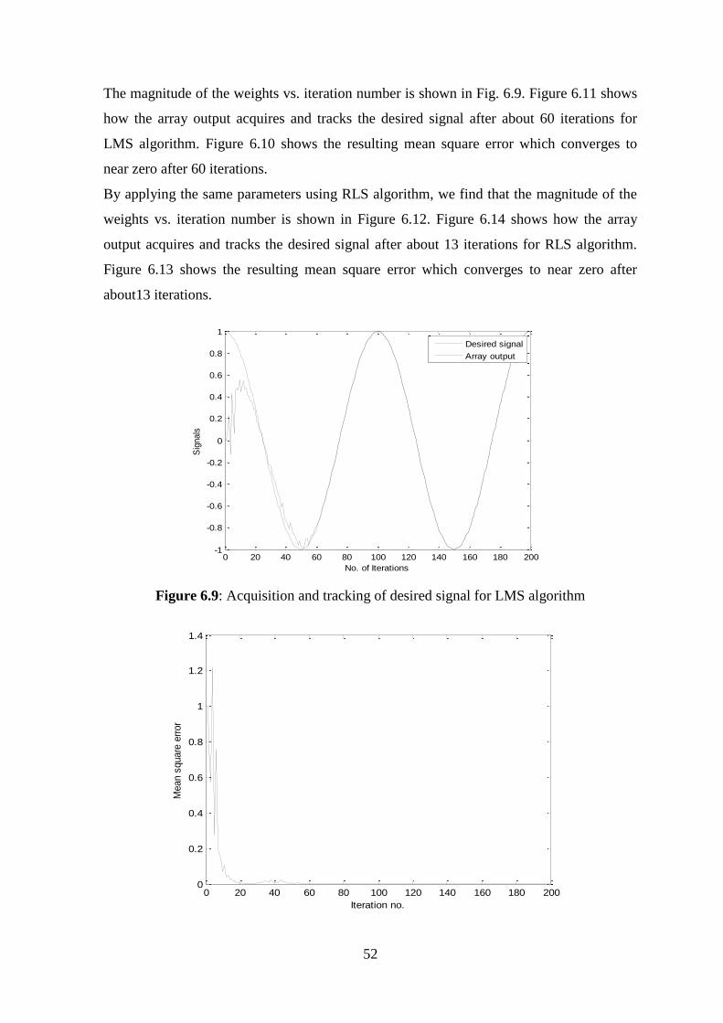
52
The magnitude of the weights vs. iteration number is shown in Fig. 6.9. Figure 6.11 shows
how the array output acquires and tracks the desired signal after about 60 iterations for
LMS algorithm. Figure 6.10 shows the resulting mean square error which converges to
near zero after 60 iterations.
By applying the same parameters using RLS algorithm, we find that the magnitude of the
weights vs. iteration number is shown in Figure 6.12. Figure 6.14 shows how the array
output acquires and tracks the desired signal after about 13 iterations for RLS algorithm.
Figure 6.13 shows the resulting mean square error which converges to near zero after
about13 iterations.
Figure 6.9: Acquisition and tracking of desired signal for LMS algorithm
0 20 40 60 80 100 120 140 160 180 200-1
-0.8
-0.6
-0.4
-0.2
0
0.2
0.4
0.6
0.8
1
No. of Iterations
Sig
nals
Desired signal
Array output
0 20 40 60 80 100 120 140 160 180 2000
0.2
0.4
0.6
0.8
1
1.2
1.4
Iteration no.
Mean s
quare
err
or
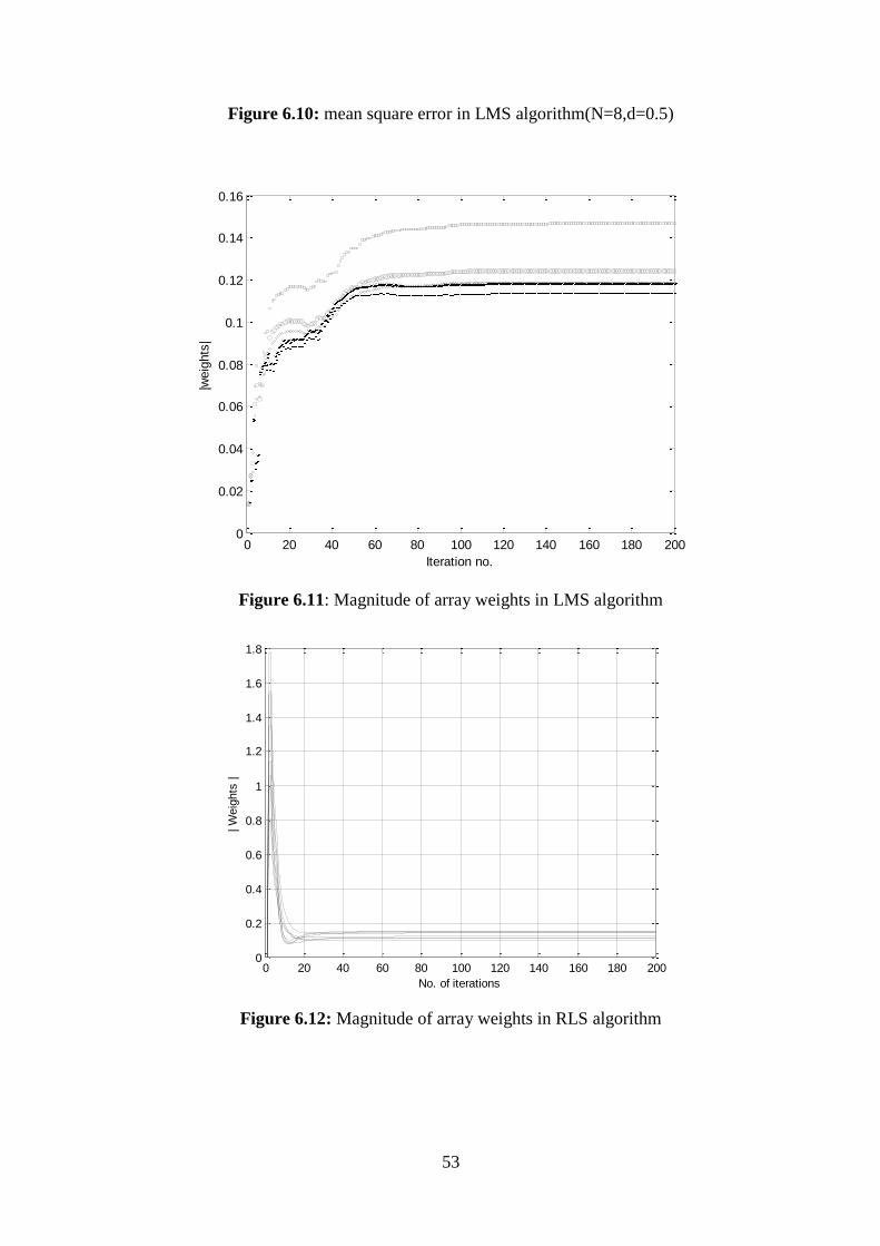
53
Figure 6.10: mean square error in LMS algorithm(N=8,d=0.5)
Figure 6.11: Magnitude of array weights in LMS algorithm
Figure 6.12: Magnitude of array weights in RLS algorithm
0 20 40 60 80 100 120 140 160 180 2000
0.02
0.04
0.06
0.08
0.1
0.12
0.14
0.16
Iteration no.
|weig
hts
|
0 20 40 60 80 100 120 140 160 180 2000
0.2
0.4
0.6
0.8
1
1.2
1.4
1.6
1.8
No. of iterations
| W
eig
hts
|
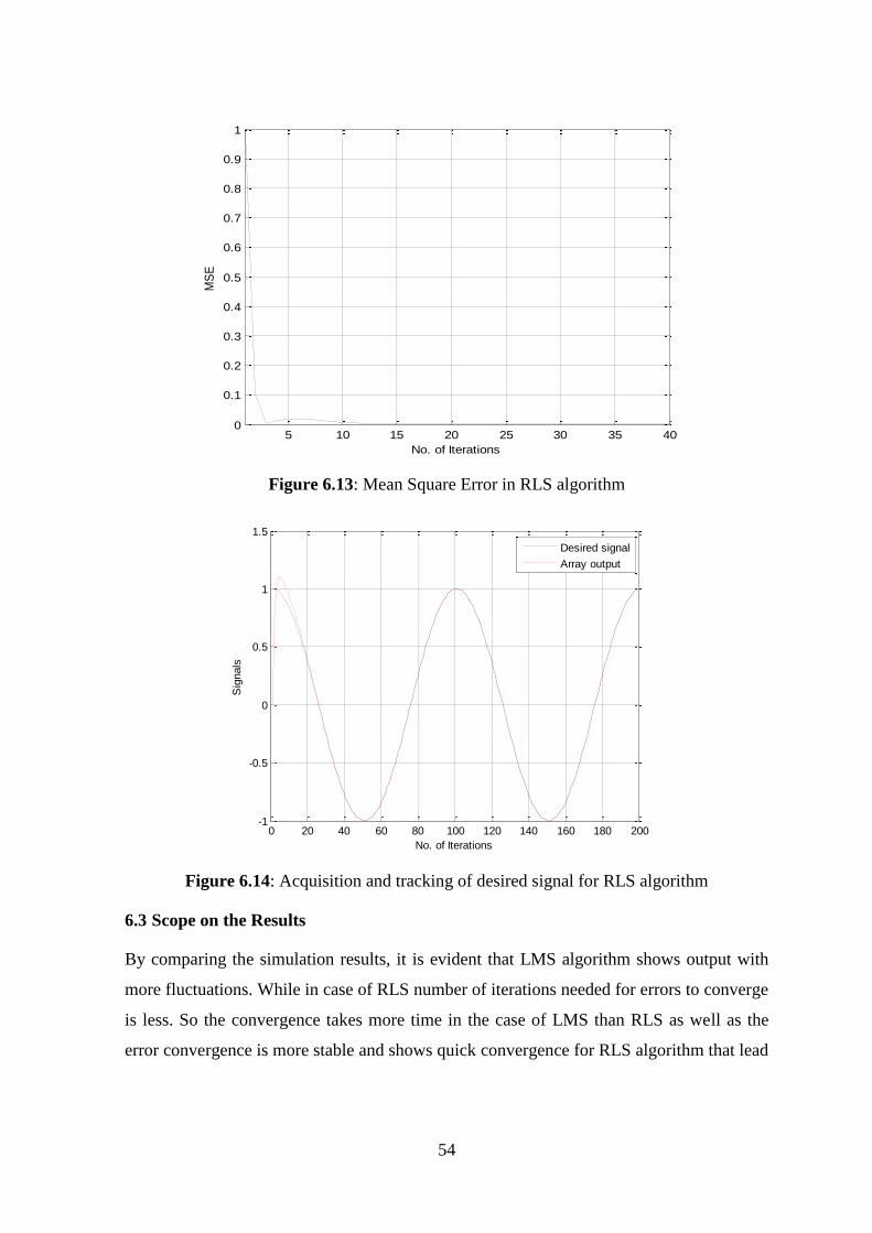
54
Figure 6.13: Mean Square Error in RLS algorithm
Figure 6.14: Acquisition and tracking of desired signal for RLS algorithm
6.3 Scope on the Results
By comparing the simulation results, it is evident that LMS algorithm shows output with
more fluctuations. While in case of RLS number of iterations needed for errors to converge
is less. So the convergence takes more time in the case of LMS than RLS as well as the
error convergence is more stable and shows quick convergence for RLS algorithm that lead
5 10 15 20 25 30 35 400
0.1
0.2
0.3
0.4
0.5
0.6
0.7
0.8
0.9
1
No. of Iterations
MS
E
0 20 40 60 80 100 120 140 160 180 200-1
-0.5
0
0.5
1
1.5
No. of Iterations
Sig
nals
Desired signal
Array output
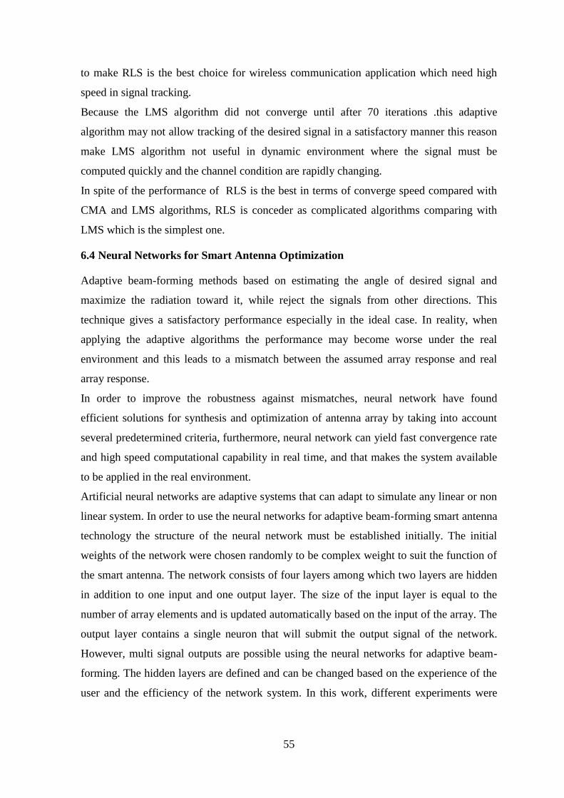
55
to make RLS is the best choice for wireless communication application which need high
speed in signal tracking.
Because the LMS algorithm did not converge until after 70 iterations .this adaptive
algorithm may not allow tracking of the desired signal in a satisfactory manner this reason
make LMS algorithm not useful in dynamic environment where the signal must be
computed quickly and the channel condition are rapidly changing.
In spite of the performance of RLS is the best in terms of converge speed compared with
CMA and LMS algorithms, RLS is conceder as complicated algorithms comparing with
LMS which is the simplest one.
6.4 Neural Networks for Smart Antenna Optimization
Adaptive beam-forming methods based on estimating the angle of desired signal and
maximize the radiation toward it, while reject the signals from other directions. This
technique gives a satisfactory performance especially in the ideal case. In reality, when
applying the adaptive algorithms the performance may become worse under the real
environment and this leads to a mismatch between the assumed array response and real
array response.
In order to improve the robustness against mismatches, neural network have found
efficient solutions for synthesis and optimization of antenna array by taking into account
several predetermined criteria, furthermore, neural network can yield fast convergence rate
and high speed computational capability in real time, and that makes the system available
to be applied in the real environment.
Artificial neural networks are adaptive systems that can adapt to simulate any linear or non
linear system. In order to use the neural networks for adaptive beam-forming smart antenna
technology the structure of the neural network must be established initially. The initial
weights of the network were chosen randomly to be complex weight to suit the function of
the smart antenna. The network consists of four layers among which two layers are hidden
in addition to one input and one output layer. The size of the input layer is equal to the
number of array elements and is updated automatically based on the input of the array. The
output layer contains a single neuron that will submit the output signal of the network.
However, multi signal outputs are possible using the neural networks for adaptive beam-
forming. The hidden layers are defined and can be changed based on the experience of the
user and the efficiency of the network system. In this work, different experiments were
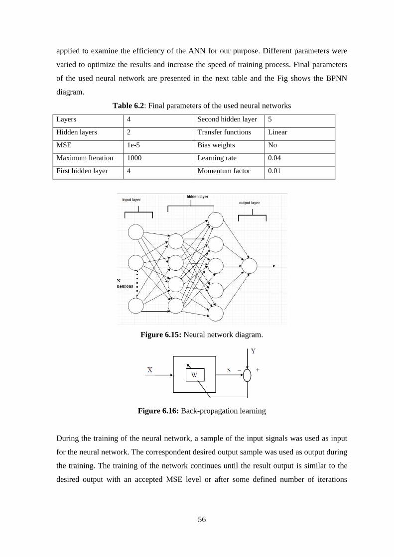
56
applied to examine the efficiency of the ANN for our purpose. Different parameters were
varied to optimize the results and increase the speed of training process. Final parameters
of the used neural network are presented in the next table and the Fig shows the BPNN
diagram.
Table 6.2: Final parameters of the used neural networks
Layers 4 Second hidden layer 5
Hidden layers 2 Transfer functions Linear
MSE 1e-5 Bias weights No
Maximum Iteration 1000 Learning rate 0.04
First hidden layer 4 Momentum factor 0.01
Figure 6.15: Neural network diagram.
Figure 6.16: Back-propagation learning
During the training of the neural network, a sample of the input signals was used as input
for the neural network. The correspondent desired output sample was used as output during
the training. The training of the network continues until the result output is similar to the
desired output with an accepted MSE level or after some defined number of iterations
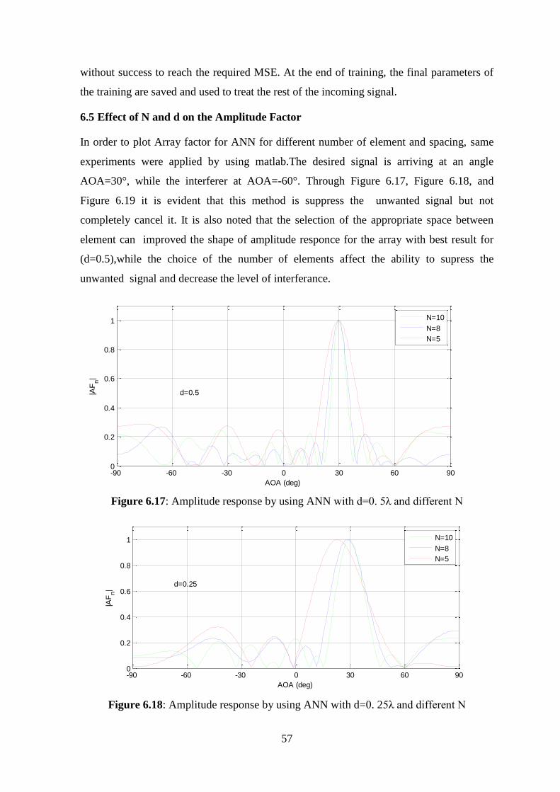
57
without success to reach the required MSE. At the end of training, the final parameters of
the training are saved and used to treat the rest of the incoming signal.
6.5 Effect of N and d on the Amplitude Factor
In order to plot Array factor for ANN for different number of element and spacing, same
experiments were applied by using matlab.The desired signal is arriving at an angle
AOA=30°, while the interferer at AOA=-60°. Through Figure 6.17, Figure 6.18, and
Figure 6.19 it is evident that this method is suppress the unwanted signal but not
completely cancel it. It is also noted that the selection of the appropriate space between
element can improved the shape of amplitude responce for the array with best result for
(d=0.5),while the choice of the number of elements affect the ability to supress the
unwanted signal and decrease the level of interferance.
Figure 6.17: Amplitude response by using ANN with d=0. 5λ and different N
Figure 6.18: Amplitude response by using ANN with d=0. 25λ and different N
-90 -60 -30 0 30 60 900
0.2
0.4
0.6
0.8
1
AOA (deg)
|AF
n|
d=0.5
N=10
N=8
N=5
-90 -60 -30 0 30 60 900
0.2
0.4
0.6
0.8
1
AOA (deg)
|AF
n|
d=0.25
N=10
N=8
N=5
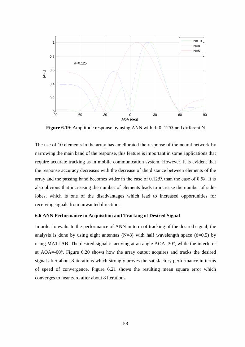
58
Figure 6.19: Amplitude response by using ANN with d=0. 125λ and different N
The use of 10 elements in the array has ameliorated the response of the neural network by
narrowing the main band of the response, this feature is important in some applications that
require accurate tracking as in mobile communication system. However, it is evident that
the response accuracy decreases with the decrease of the distance between elements of the
array and the passing band becomes wider in the case of 0.125λ than the case of 0.5λ. It is
also obvious that increasing the number of elements leads to increase the number of side-
lobes, which is one of the disadvantages which lead to increased opportunities for
receiving signals from unwanted directions.
6.6 ANN Performance in Acquisition and Tracking of Desired Signal
In order to evaluate the performance of ANN in term of tracking of the desired signal, the
analysis is done by using eight antennas (N=8) with half wavelength space (d=0.5) by
using MATLAB. The desired signal is arriving at an angle AOA=30°, while the interferer
at AOA=-60°. Figure 6.20 shows how the array output acquires and tracks the desired
signal after about 8 iterations which strongly proves the satisfactory performance in terms
of speed of convergence, Figure 6.21 shows the resulting mean square error which
converges to near zero after about 8 iterations
-90 -60 -30 0 30 60 900
0.2
0.4
0.6
0.8
1
AOA (deg)
|AF
n|
d=0.125
N=10
N=8
N=5
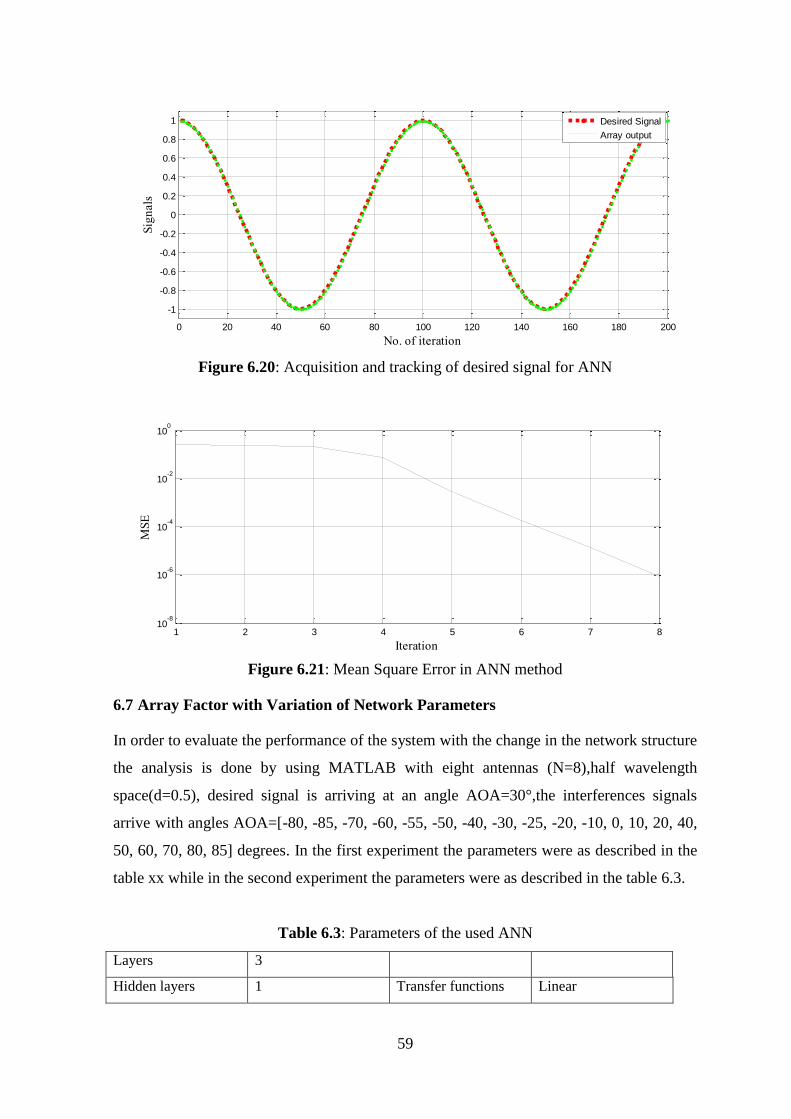
59
Figure 6.20: Acquisition and tracking of desired signal for ANN
Figure 6.21: Mean Square Error in ANN method
6.7 Array Factor with Variation of Network Parameters
In order to evaluate the performance of the system with the change in the network structure
the analysis is done by using MATLAB with eight antennas (N=8),half wavelength
space(d=0.5), desired signal is arriving at an angle AOA=30°,the interferences signals
arrive with angles AOA=[-80, -85, -70, -60, -55, -50, -40, -30, -25, -20, -10, 0, 10, 20, 40,
50, 60, 70, 80, 85] degrees. In the first experiment the parameters were as described in the
table xx while in the second experiment the parameters were as described in the table 6.3.
Table 6.3: Parameters of the used ANN
Layers 3
Hidden layers 1 Transfer functions Linear
0 20 40 60 80 100 120 140 160 180 200
-1
-0.8
-0.6
-0.4
-0.2
0
0.2
0.4
0.6
0.8
1
No. of iteration
Sig
nals
Desired Signal
Array output
1 2 3 4 5 6 7 810
-8
10-6
10-4
10-2
100
Iteration
MS
E
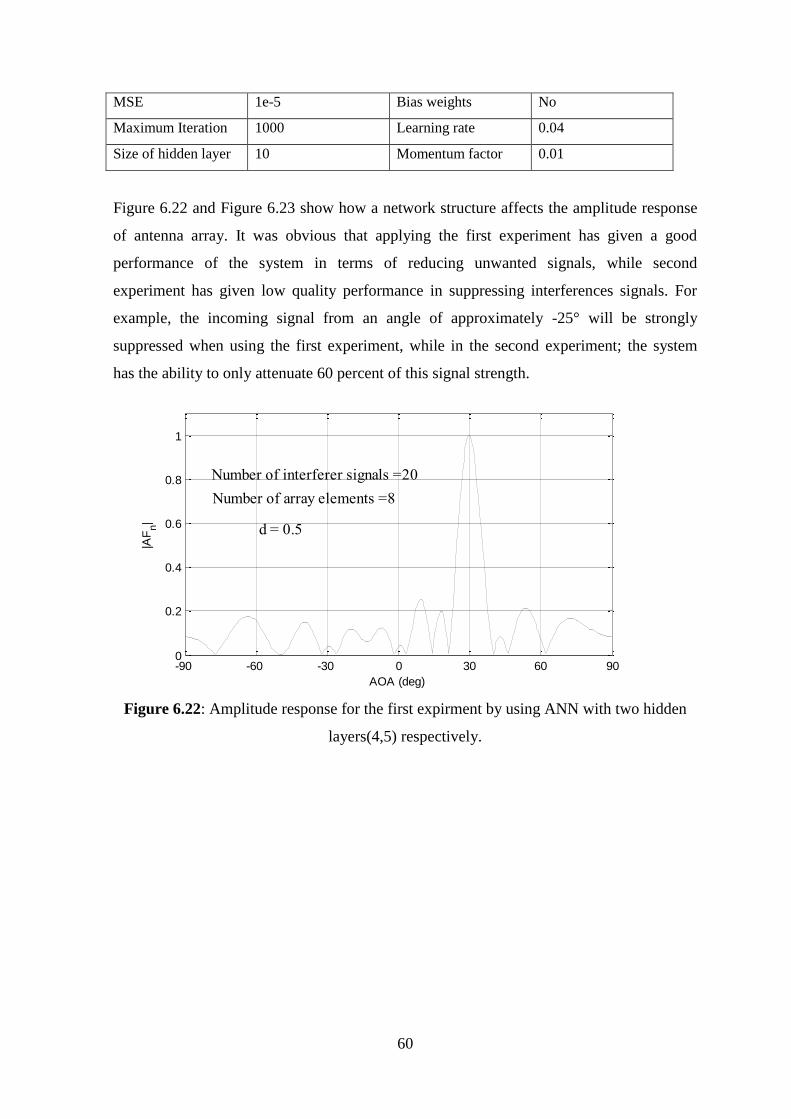
60
MSE 1e-5 Bias weights No
Maximum Iteration 1000 Learning rate 0.04
Size of hidden layer 10 Momentum factor 0.01
Figure 6.22 and Figure 6.23 show how a network structure affects the amplitude response
of antenna array. It was obvious that applying the first experiment has given a good
performance of the system in terms of reducing unwanted signals, while second
experiment has given low quality performance in suppressing interferences signals. For
example, the incoming signal from an angle of approximately -25° will be strongly
suppressed when using the first experiment, while in the second experiment; the system
has the ability to only attenuate 60 percent of this signal strength.
Figure 6.22: Amplitude response for the first expirment by using ANN with two hidden
layers(4,5) respectively.
-90 -60 -30 0 30 60 900
0.2
0.4
0.6
0.8
1
AOA (deg)
|AF
n|
Number of interferer signals =20
Number of array elements =8
d = 0.5
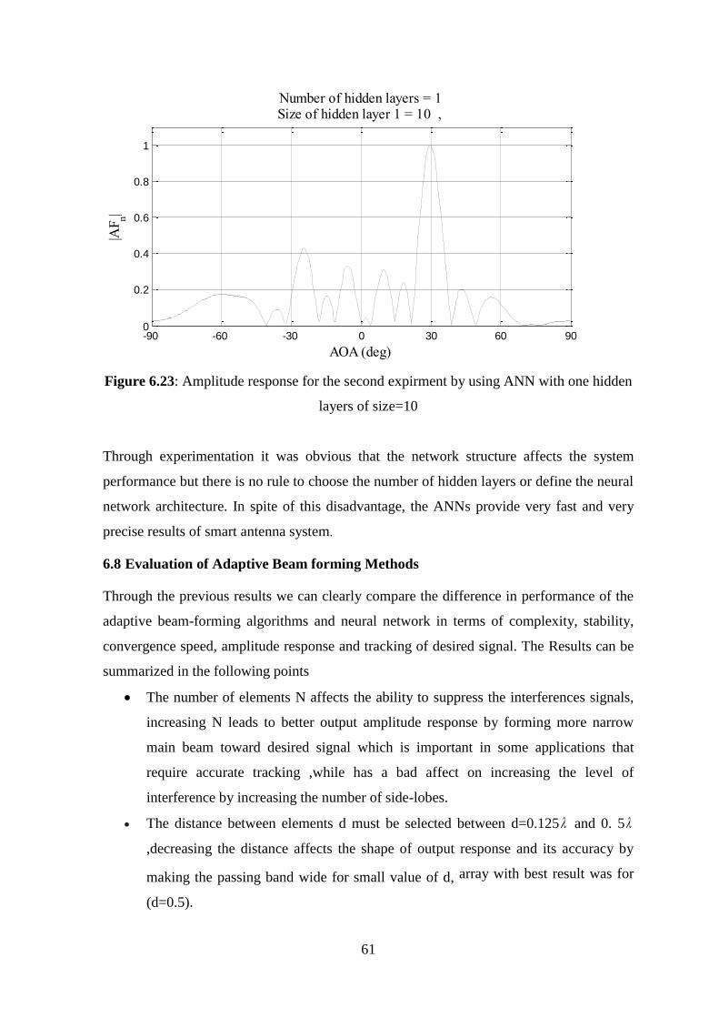
61
Figure 6.23: Amplitude response for the second expirment by using ANN with one hidden
layers of size=10
Through experimentation it was obvious that the network structure affects the system
performance but there is no rule to choose the number of hidden layers or define the neural
network architecture. In spite of this disadvantage, the ANNs provide very fast and very
precise results of smart antenna system.
6.8 Evaluation of Adaptive Beam forming Methods
Through the previous results we can clearly compare the difference in performance of the
adaptive beam-forming algorithms and neural network in terms of complexity, stability,
convergence speed, amplitude response and tracking of desired signal. The Results can be
summarized in the following points
The number of elements N affects the ability to suppress the interferences signals,
increasing N leads to better output amplitude response by forming more narrow
main beam toward desired signal which is important in some applications that
require accurate tracking ,while has a bad affect on increasing the level of
interference by increasing the number of side-lobes.
The distance between elements d must be selected between d=0.125 and 0. 5
,decreasing the distance affects the shape of output response and its accuracy by
making the passing band wide for small value of d, array with best result was for
(d=0.5).
-90 -60 -30 0 30 60 900
0.2
0.4
0.6
0.8
1
AOA (deg)
|AF
n|
Number of hidden layers = 1Size of hidden layer 1 = 10 ,
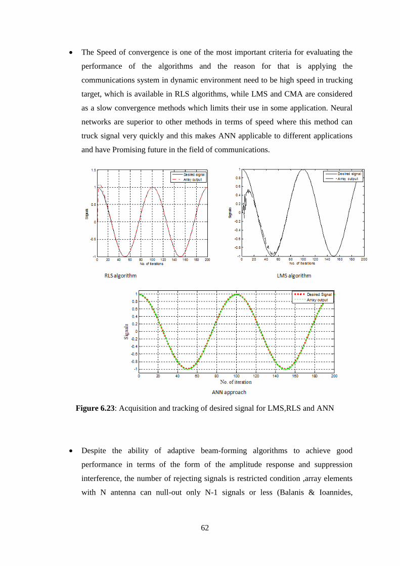
62
The Speed of convergence is one of the most important criteria for evaluating the
performance of the algorithms and the reason for that is applying the
communications system in dynamic environment need to be high speed in trucking
target, which is available in RLS algorithms, while LMS and CMA are considered
as a slow convergence methods which limits their use in some application. Neural
networks are superior to other methods in terms of speed where this method can
truck signal very quickly and this makes ANN applicable to different applications
and have Promising future in the field of communications.
Figure 6.23: Acquisition and tracking of desired signal for LMS,RLS and ANN
Despite the ability of adaptive beam-forming algorithms to achieve good
performance in terms of the form of the amplitude response and suppression
interference, the number of rejecting signals is restricted condition ,array elements
with N antenna can null-out only N-1 signals or less (Balanis & Ioannides,
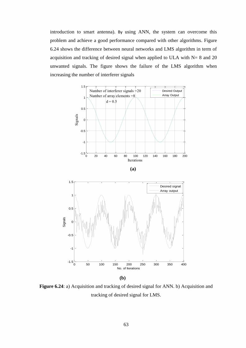
63
introduction to smart antenna). By using ANN, the system can overcome this
problem and achieve a good performance compared with other algorithms. Figure
6.24 shows the difference between neural networks and LMS algorithm in term of
acquisition and tracking of desired signal when applied to ULA with N= 8 and 20
unwanted signals. The figure shows the failure of the LMS algorithm when
increasing the number of interferer signals
(a)
(b)
Figure 6.24: a) Acquisition and tracking of desired signal for ANN. b) Acquisition and
tracking of desired signal for LMS.
0 20 40 60 80 100 120 140 160 180 200-1.5
-1
-0.5
0
0.5
1
1.5
Sig
nals
Iterations
Number of interferer signals =20
Number of array elements =8
d = 0.5
Desired Output
Array Output
0 50 100 150 200 250 300 350 400-1.5
-1
-0.5
0
0.5
1
1.5
No. of Iterations
Sig
nals
Desired signal
Array output
64
CONCLUSIONS
Recent years have witnessed remarkable exploitation of smart antenna technology in the
development of wireless communications industry due to the high efficiency of these
systems, which rely on the integration of antenna array with digital signal processing unit
to increase the efficiency of systems in terms of the range, speed, and capacity. It was
evident that the adaptive beamforming technique was the major responsible for controls the
directionality of the radiation patterns in both the receiver and transmitter, this signal
processing technique has the ability to shape and direct the main beam of radiation toward
the desired target while suppress other unwanted signals by using adaptive algorithms .
This work compared and analyzed three popular adaptive techniques including LMS, RLS,
and CMA with Back-propagation Neural Networks as a powerful tool in optimization of
the antenna array performance
The Results obtained could be summarized as follows:
LMS algorithms is the simplest method with reasonable performance in term of
stability, and suppression of the interferences, furthermore, it can be considered as
an ideal choice for many applications that need the robustness and simplicity,
However LMS cannot be considered the best choice with regard to speed, since it
needs a high number of iterations before convergence.
RLS algorithms has a faster convergence and a good performance for the
suppression of interference compared to other conventional adaptive beamforming
algorithms, so it is considered as a reasonable choice for some applications where
quick tracking of the desired signal is required, However, the complexity of
calculations in this method is one of the main obstacles limiting its use in some
applications.
Some techniques are more suitable to be used in situations where no reference
signal is available. These techniques are said to be blind to the received signal’s
exact content. CMA algorithm is one of the main algorithms of this category. The
results obtained showed that this method is not the best in terms of speed and
suppression of interference signals.
The performance of these algorithms is discussed and experimented with a series of
simulations for varying parameter of uniform linear arrays such as, number of antenna
65
elements, and the spacing between elements in order to discover the extent effect of the
array geometries on the performance.
Finally, a neural network back propagation algorithm is proposed to overcome tracking
problem and other limitations in using the conventional methods in light of the results
obtained previously by using (LMS, RLS, and CMA) algorithms, The use of ANN in
beamforming has proved better performance; the fastest convergence to the desired signal
and flexibility, Moreover, this method has ability to reject greater number of interferer
compared with other algorithms, which leads to making the SAS applicable to different
applications.
66
REFERENCES
Abdallah, A., Joumaa, C., & Kadry, S. (N.d.). Design and Performance study of Smart
Antenna Systems for WIMAX applications. Kuwait.
Antenna Basic Concepts. (s.d.). Found at: www.pulseelectronics.com/products/antennas.
Azad, D. M., & Ahmed, A. H. (2010, October). Development of Smart Antenna for Future
Generation Wireless. International Journal of Computer Science and Network
Security, 212-222.
Balanis, C. A., & Ioannides, P. I. (2007). Introduction to smart antenna. Arizona.
Bellofiore, S., Balanis, C. f., Foufz, J., & Spanias, a. A. (2002). Smart-Antenna Systems
for Mobile communication network. IEEE Antenna’s and Propagation Magazine
Part1, 145-154.
Bevelacqua, P. J. (2008). Antenna Arrays: Performance Limits And Geometry. Arizona.
Bevelacqua, P. J. (2009). Introduction to Antenna Array Geometry. Found on antenna-
theory: http://www.antenna-theory.com/arrays/geometry/basics.php
Bevelacqua, P. J. (2009). The Array Factor. Found on Antenna-Theory.com:
http://www.antenna-theory.com/arrays/arrayfactor.php
Boyle, k., & Huang, Y. (2008). Antenna from theory to practice. UK: Jouhn wiley&sons
LTD.
Chang, D.-C., & Hu, C.-N. (2012). Smart Antennas for Advanced Communication
Systems. Proceedings of the IEEE, 2233 - 2249.
doi:10.1109/JPROC.2012.2187409
Christodoulou, C. G., Tawk, Y., Lane, S. A., & Erwin, S. R. (2012). Reconfigurable
Antennas for Wireless and Space Applications. IEEE proceedings, 100(7), 2250 -
2261. doi:10.1109/JPROC.2012.2188249
Cohen, D. I. (2003). Digital Speech Processing in Noisy. Australia.
Das, S. (s.d.). Smart Antenna Design for Wireless Communication using. Rourkela.
Fonda, C., & Zennaro, M. (2004). The Radio Laboratory Handbook. International Centre
for Theoritical Physics ICTP.
Fung, C. ( 2011). Basic Antenna Theory and Application. United States: Worcester
Polytechnic Institute Univesity.
Fyfe, C. (1996). Artificial Neural Networks. University Of Paisley.

67
Garcia, L. G., Ariet, L. D., & Rodriguez-Osorio, R. M. (2004). Implementation of a neural
network-based digital beamformer for a UMTS smart antenna. IEEE Sensor Array
and Multichannel Signal Processing Workshop Proceedings, 119-123.
doi:10.1109/SAM.2004.1502920
Goldsmith, A. (2004). Wireless Communications. California.
Gross, F. B. (2005). Smart Antennas for wireless communication. Virginia: The McGraw-
Hill Companies.
Haykin, S. (2002). Adaptive filter theory (ed. 4). Ontario, Canada: Pearson education asia.
Hreshee, D. S. (2013, October). LMS Algorithm for Optimizing the Phased Array Antenna
Radiation Pattern. JOURNAL OF TELECOMMUNICATIONS, 20-24.
Hreshee, S. (2013). LMS Algorithm for Optimizing the Phased Array Antenna Radiation
Pattern . JOURNAL OF TELECOMMUNICATIONS, 20-24.
Jain, R., Katiyar, u., & Agrawal, N. (2011). Smart Antenna for Cellular Mobile
Communication. VSRD International Journal of Electrical, Electronics & Comm.
Engg, 530-541.
Joseph C.Libertii, J., & S.Rappaport, T. (1999). Smart Antenna for Wireless
Communication: IS-95 and Third Generation CDMA Applications. New Jersey:
Prentice Hall .
Karmakar, N. C. (2011). Handbook of Smart Antennas for RFID Systems. John Wiley &
Sons.
Kavak, A., Yigit, H., & Ertunc, H. M. (2005). Using adaline neural network for
performance improvement of smart antennas in TDD wireless communications.
IEEE Transactions on Neural Networks, 1616 - 1625.
doi:10.1109/TNN.2005.857947
Kawitkar, R., & Wakdi, D. (2005, September). Advances in smart antenna system. Journal
in Scientific &Industrial research, 660-665.
Khashman, A. (1999). Automatic Edge Detection of DNA Bands in Autoradiograph
Images. International Symposium on Industrial Electronics (pp. 1184 - 1188).
Bled: IEEE. doi:10.1109/ISIE.1999.796864
Khashman, A., & Dimililer, K. (2007). Neural Networks Arbitration for Optimum DCT
Image Compression. International Conference on Computer as Tool (pp. 151 -
156). Warsaw: IEEE. doi:10.1109/EURCON.2007.4400236
68
Khasim, N. S., Krishna, Y., & Thati., J. (s.d.). Analysis of Different Tapering Techniques
for Efficient Radiation Pattern. e-Journal of Science & Technology, 47-53.
Krose, B., & Smagt, P. v. (1996). An Introduction to Neural Networks (éd. eighth). (U. o.
Amsterdam, Éd.) Amsterdam: University of Amsterdam.
Mallaparapu, U., Nalini, K., Ganesh, P., Vishnu, T. R., Khan, P. H., Lakshmi, D., &
Madhav., B. (2011, March). Non-Blind Adaptive Beam Forming Algorithms for
Smart Antenna. International Journal of Research and Reviews in Applied
Sciences, 491-496.
merad, L., Bendimerad, F., & Sidi Mohamed Meriah, S. A. (2007). Neural Networks for
Synthesis and Optimization of Antenna Arrays. Journal of Radioengineering, 23-
30.
Olenewa, J. (2013). Guide to Wireless Communications. Cengage Learning.
Orakwue, S. I., Ngah, R., Rahman, T. A., & Hashim, S. Z. (2014). Neural network based
switch beam smart antenna. IEEE Conference Publications, 292-296.
doi:10.1109/APWiMob.2014.6920300
Pei, B., Han, H., Sheng, Y., & Qiu, B. (2013). Research on smart antenna beamforming by
generalized regression neural network. IEEE conference publications, 1-4.
doi:10.1109/ICSPCC.2013.6663990
Rahaman, D. M., Hossain, M. M., & Rana, M. M. (2013). Least Mean Square (LMS) for
Smart Antenna. Universal Journal of Communications and Network, 16-21.
Ramineni, 1., Sagar, G., K.Abhishek Jain, M. G., T.V.Ramakrishna, & Kumar, K. (2012,
may). Comparison and performance evaluation of different adaptive beam forming
algorithms in wireless communications with smart antenna. International Journal
of Engineering Research(3), 630-633.
Rani, C. S., Subbaiah, P. V., Reddy, K. C., & Rani, S. S. (2009, AUGUST). Lms and Rls
Algorithms for Smart Antennas in a W-Cdma Mobile Communication
Environment. ARPN Journal of Engineering and Applied Sciences, 4, 78-88.
RAO, A. P., & SARMA, N. (2014). Adaptive Beamforming Algorithms for Smart Antenna
Systems. WSEAS TRANSACTIONS on COMMUNICATIONS, 44-50.
Rawat, A., Yadav, R. N., & Shrivastava, S. C. (2009). Neural Modeling of 15 Element
Dynamic Phased Array Smart Antenna. IEEE publications, 45 - 48.
doi:10.1109/ACT.2009.21
Rojas, R. (1996). Neural Networks, a systematic introduction. Berlin: Springer-Verlag.
69
Sadhu, T. (2012, Dec 2). machine learning. Seen on Jul 20, 2016, at Durofy:
http://durofy.com/machine-learning-introduction-to-the-artificial-neural-
network/neuron-2/
Saleh, A., AL-Ali, A., & Alssarn, M. (2013). Neural Networks Application in Smart
Antenna Systems For Obtaining an Optimal Output. Tishreen University Journal
for Research and Scientific Studies, 215-226.
Sallomi, A. H., & Salim, S. R. (2009). Range-Coverage Extension Using Smart Antennas
in Mobile Communications systems. Iraqi Journal of Applied Physics, 25-28.
Sarevska, M., Milovanovic, B., & Stankovic, Z. (2004). Alternative signal detection for
neural network-based smart antenna. Neural Network Applications in Electrical
Engineering, IEEE, 85-89. doi:10.1109/NEUREL.2004.1416541
Stevanovic, I., Skrivervik, A., & Mosig, J. R. (2003). Smart Antenna Systems for Mobile
Communications. lausanne.
(Rappaport, 2002). The cellular concept-system design fundamental. Dans T. S. Rappaport,
Wireless Communications principle and practice (pp. 25-67).
Trivedi, S. (2008, feb 15). The Motivation behind Artificial Neural Networks. Seen on 7
27, 2016, Onionesque reality:
https://onionesquereality.wordpress.com/2008/02/15/the-motivation-behind-
artificial-neural-networks/
Yigit, H., Kavak, A., & Ertunc, H. .. (2004). Using Autoregressive and Adaline Neural
Network Modeling to Improve Downlink Performance of Smart Antennas.
Proceedings of IEEE international conference on mechatronics, 165-170.
doi:10.1109/ICMECH.2004.1364431
Zooghby, A. H., Christodoulou, C. G., & Georgiopoulos, M. (2000). A Neural Network-
Based Smart Antenna for Multiple Source Tracking. IEEE TRANSACTIONS ON
ANTENNAS AND PROPAGATION, 768-776.


![Enlighteneprints.gla.ac.uk/218294/1/218294.pdfAdaptive Beamforming is a widely used technique in wire-less communication [1], acoustic sensors array [2], medical imaging [3] and other](https://static.fdocuments.in/doc/165x107/60d1a421606c0704fb1f52b7/adaptive-beamforming-is-a-widely-used-technique-in-wire-less-communication-1.jpg)