Adaptive Beamforming Applied to Medical Ultrasound · PDF file1606 ieee transactions on...

1606 ieee transactions on ultrasonics, ferroelectrics, and frequency control, vol. 54, no. 8, august 2007

Adaptive Beamforming Applied to MedicalUltrasound Imaging

Johan-Fredrik Synnevag, Student Member, IEEE, Andreas Austeng, Member, IEEE,and Sverre Holm, Senior Member, IEEE

Abstract—We have applied the minimum variance (MV)adaptive beamformer to medical ultrasound imaging andshown significant improvement in image quality comparedto delay-and-sum (DAS). We demonstrate reduced main-lobe width and suppression of sidelobes on both simulatedand experimental RF data of closely spaced wire targets,which gives potential contrast and resolution enhancementin medical images. The method is applied to experimentalRF data from a heart phantom, in which we show increasedresolution and improved definition of the ventricular walls.

A potential weakness of adaptive beamformers is sensi-tivity to errors in the assumed wavefield parameters. Welook at two ways to increase robustness of the proposedmethod; spatial smoothing and diagonal loading. We showthat both are controlled by a single parameter that canmove the performance from that of a MV beamformer tothat of a DAS beamformer. We evaluate the sensitivity tovelocity errors and show that reliable amplitude estimatesare achieved while the mainlobe width and sidelobe levelsare still significantly lower than for the conventional beam-former.

I. Introduction

Delay-and-sum (DAS) beamforming is the standardtechnique in medical ultrasound imaging. An image is

formed by transmitting a narrow beam in a number of an-gles and dynamically delaying and summing the receivedsignals from all channels. The sidelobe level of the DASbeamformer can be controlled using aperture shading, re-sulting in increased contrast at the expense of resolution.In contrast to the predetermined shading in DAS, adap-tive beamformers use the recorded wavefield to computethe aperture weights. By suppressing interfering signalsfrom off-axis directions and allowing large sidelobes in di-rections in which there is no received energy, the adaptivebeamformers can increase resolution.

The minimum variance (MV) adaptive beamformer [1],[2] and subspace-based methods have mostly been stud-ied in narrowband applications. Extensions to broadbandimaging include preprocessing with focusing- and spatial-resampling filters, allowing narrowband methods to beused on broadband data [3], [4]. The MV beamformer hasbeen applied to medical ultrasound imaging by several au-thors [5]–[9]. Mann and Walker [5] have used a constrainedadaptive beamformer on experimental data of a singlepoint-target and a cyst phantom demonstrating improved

Manuscript received April 30, 2006; accepted October 18, 2006.The authors are with the University of Oslo, Department of Infor-

matics, Oslo, Norway (e-mail: [email protected]).Digital Object Identifier 10.1109/TUFFC.2007.431

contrast and resolution. Sasso and Cohen-Bacrie [6] haveapplied a MV beamformer on a simulated dataset, show-ing improved contrast in the final image. Viola and Walker[9] have investigated use of several adaptive beamformerson simulated data and demonstrated improved resolution.Wang et al. [7] have applied a robust MV beamformer tomedical ultrasound imaging using a synthetic aperture fo-cusing approach. In their method, the spatial covariancematrix, which is required to find the optimal apertureshading, is calculated by averaging appropriately delayeddata from each individual transmit element. Although thismethod allows dynamic focus on both transmission and re-ception, the loss in signal-to-noise ratio (SNR) caused bysynthetic aperture focusing may be unacceptable in med-ical imaging applications. Also, data captured with differ-ent transmit elements may not be coherent due to tar-get motion. In [8], we show preliminary results from thepresent method, in which full dynamic focus was appliedthrough synthetic focus of individual transmitters. In thispaper, we apply fixed focus on transmission. That allowsus to evaluate the performance of the beamformer out-side the transmit focal point, giving more realistic resultsfor medical ultrasound imaging. We also consider ways ofincreasing the robustness of the MV beamformer, whichensures reliable amplitude estimates and at the same timeimproves performance.

In Section II, we present the method and show how ro-bustness is achieved through either spatial smoothing ordiagonal loading. In Section III we compare the MV beam-former to DAS on simulated and experimental RF datafrom closely spaced wire targets, and on experimental RFdata of a heart phantom. We also evaluate the sensitivityof the method to errors in acoustic velocity and show thatreliable amplitude estimates can be achieved by either ofthe robust methods. We discuss our findings in Section IVand draw conclusions in Section V.

II. Methods

A. Signal Model and Minimum Variance Beamformer

We assume an array of M elements, each recording asignal xm(t). We consider P + 1 scatterers, each reflectinga signal, sp(t). We assume that s0(t) originates from thefocal point of the receiver, and that the other reflectors aresources of interference. Under these assumptions, the mthtime-delayed channel can be described as:

0885–3010/$25.00 c© 2007 IEEE

synnevag et al.: beamforming applied to medical ultrasound imaging 1607

xm(t) =1

rm,0s0(t) +

P∑p=1

1rm,p

sp(t) ∗ δ(t − τm,p) + nm(t),(1)

where rm,p is the distance from reflector p to sensor m, δ(t)is the Dirac delta-function, τm,p is the delay from reflectorp to sensor m, nm(t) is noise on channel m, and (∗) is theconvolution operator. The M observations are ordered ina vector:

X(t) =

⎡⎢⎢⎢⎣

x0(t)x1(t)

...xM−1(t)

⎤⎥⎥⎥⎦ , (2)

which represents the observed wavefield. After delayingeach channel to focus at a point in the image, the goal ofthe adaptive beamformer is to compute the optimal aper-ture shading before combining the channels. The outputof the beamformer is a weighted sum of the spatial mea-surements:

z(t) =M−1∑m=0

wm(t)xm(t) = w(t)HX(t), (3)

where wm(t) is the aperture weight for sensor m, andw(t) = [w0(t) w1(t) · · ·wM−1(t)]H . The minimum variancebeamformer seeks to minimize the variance (power) of z(t):

P (t) = E[|z(t)|2], (4)

while maintaining unit gain in the focal point. This opti-mization problem can be formulated as:

minw(t)

w(t)HR(t)w(t),

subject to w(t)Ha = 1,(5)

where:

R(t) = E[X(t)X(t)H

], (6)

is the spatial covariance matrix and a is the equivalent ofthe steering vector in narrowband applications. Becausethe data already have been delayed to focus at the pointof interest, a is simply a vector of ones. The solution to(5) is:

w(t) =R(t)−1a

aHR(t)−1a. (7)

Applying these weights to (3) gives the MV amplitude es-timate.

B. Estimation of the Spatial Covariance Matrix

In practice, the covariance matrix, R(t), in (7) is re-placed by the sample covariance matrix, R(t). Because thetransmitted pulses in medical ultrasound imaging are shortand nonstationary, R(t) is rapidly changing with time.

Hence, the estimate must be calculated from a single, oronly a few, temporal samples. If synthetic aperture focus-ing (SAFT) is used as in [7], the estimate can be obtainedby averaging the covariance matrices of appropriately de-layed observations from each individual transmit element.Target motion and SNR requirements, however, may pro-hibit use of SAFT in practical medical ultrasound systemsand require all elements to transmit simultaneously. To ob-tain a good estimate, we instead use spatial smoothing [10],in which the array is divided into overlapping subarrays,and the covariance matrices for all subarrays are averaged.This technique also is used to avoid signal cancellation innarrowband applications when sources are correlated orcoherent. The estimated covariance matrix at time t thenbecomes:

R(t) =1

M − L + 1

M−L∑l=0

Xl(t)XH

l (t), (8)

where:

Xl(t) =

⎡⎢⎢⎢⎣

xl(t)xl+1(t)

...xl+L−1(t)

⎤⎥⎥⎥⎦ , (9)

and L is the subarray length. By using R(t) in (7) we seethat the number of coefficients in w(t) is reduced, whichlimits the degrees of freedom to suppress interfering sig-nals and noise. There is then a trade-off between accurateestimation of the covariance matrix and the length of thespatial filter. As we discuss in Section III, decreasing thesubarray length leads to a more robust solution, but reso-lution is decreased.

After computation of the optimal aperture weights us-ing the sample covariance matrix, we obtain the amplitudeestimate as:

z(t) =1

M − L + 1

M−L∑l=0

w(t)HXl(t). (10)

The amplitude estimate can be viewed as a sum ofM − L + 1 directive elements. Hence, the minimum vari-ance solution approaches DAS as the subarray length is de-creased. The overlapping subarrays give some more weightto the central elements, corresponding to a nonuniformshading.

C. Robust Minimum Variance Beamforming

Due to the high resolution of the MV beamformer athigh SNR, a large number of scan lines may be requiredto avoid angular undersampling and to ensure robustnessagainst errors in the wavefield parameters. We expect thatsuch errors will affect the peaks in the amplitude estimatesand lead to underestimation of the reflectivity of the tar-gets. The constraint in (5) only assures that reflectionsoriginating from the focal point of the receiver are passed


with unit gain—others are suppressed. Wrong assumptionsof acoustic velocity or phase aberrations will, for instance,lead to targets appearing slightly out of focus. The MVbeamformer will try to minimize these reflections. By in-creasing robustness, we constrain the level of suppressionoutside the focal point, and allow reflections appearingslightly out of focus to pass through the beamformer.

We consider two ways to increase robustness of theproposed method in this paper; decreasing the subarraylength when computing (8), and diagonal loading of theestimated covariance matrix. As discussed in Section II,the proposed method approaches the DAS beamformer asthe subarray length, L, is decreased. In the extreme casewhere L = 1, (10) becomes the DAS solution with uni-form aperture shading. Hence, by increasing the numberof subarrays used to form the sample covariance matrix, weobtain an increasingly robust solution. However, increasedrobustness comes at the expense of resolution. The choiceof subarray length should ensure that the covariance ma-trix estimate is invertible, which sets the upper limit on Lto [11]:

L ≤ M/2. (11)

We show results for several values of L in Section III.A second common way to increase robustness of the

MV beamformer is to add a constant, ε, to the diago-nal of the covariance matrix before evaluating (7). Thismeans that R(t) is replaced by R(t) + εI. There existsseveral methods for calculating the value of ε based on theuncertainty in the model parameters [12]. We use a sim-ple approach, in which the amount of diagonal loading isproportional to the power in the received signals [13]. Wecan view diagonal loading as adding spatially white noiseto the recorded wavefield before computing the apertureweights. Increased noise level will constrain the sidelobelevels in directions in which there are no interfering sig-nals, and thereby limit the level of suppression in direc-tions in which interfering reflections appear. As white noisebecomes dominant, the MV solution approaches the DASbeamformer with uniform shading. We can see this if weconsider a wavefield of spatially white noise. The covari-ance matrix is then proportional to the identity matrix,R(t) = σ2

nI, where σ2n is the variance of the noise. From

(7) we get:

w(t) =(σ2

nI)−1aaH(σ2

nI)−1a=

aaHa

=1M

a, (12)

which is simply an unweighted sum of the elements. Inthe following results the amount of diagonal loading isfound as:

ε = ∆ · tr{R(t)}, (13)

where ∆ is a constant and tr{·} is the trace operator. Theamount of diagonal loading then is given by the power inthe received signals and the predetermined value ∆. ∆ de-termines the relative weight given to the optimal solution

in (7) and the DAS solution in (12). Setting ∆ = 1/L cor-responds to equal weighting of the two, in the sense thatthe traces of R(t) and εI are the same [13]. We also caninterpret ∆ as a parameter controlling the relative artifi-cial noise level in the data. Setting ∆ = 1/L correspondsto adding spatially white noise with the same average vari-ance as the received signals. As we will see in Section III,we obtain a robust solution using ∆ = 1/L.

We now have two ways of increasing robustness of theproposed method, which both move the performance fromthat of a MV beamformer to that of an unweighted DASbeamformer.

III. Results

We have applied the MV beamformer to both simu-lated and experimental RF data and compared the resultsto the DAS beamformer. All transmitter and receiver com-binations were simulated or recorded. The first processingsteps were common to both beamformers: We synthesizedfixed focus on transmission and dynamic focus on recep-tion by delay and sum of the recorded data from each in-dividual transmitter. Delays were implemented by upsam-pling the received signals and selecting the sample closestto the theoretically predicted delay. We then computedthe discrete time analytic signal of each channel. This wasdone to avoid symmetric beampatterns in the MV solu-tion, which could decrease resolution. The receiver chan-nels then were summed for the DAS beamformer. For theMV beamformer, the optimal aperture weights were calcu-lated and applied before summation. All MV beamformerresults used subarray length L ≤ M/2. Unless a diagonalloading parameter is given, we used ∆ = 1/100L to ensurea well conditioned covariance matrix.

A. Simulated Data

We simulated an 18.5 mm, 96 element, 4 MHz trans-ducer using Field II [14], imaging a number of pairwisereflectors located at depths 30–80 mm. The reflectorswere separated by 2 mm. Transmit focus was 60 mm.We added white, Gaussian noise to each receiver channelbefore beamforming. SNR was approximately 40 dB perchannel for the reflectors in focus.

Fig. 1(a) shows images obtained with the DAS andMV beamformers displayed over 55 dB dynamic range.Figs. 1(b)–(d) show the MV beamformer for different sub-array lengths. We see that as L increases the reflectors arebetter resolved, whereas for smaller L the image is closerto DAS. Fig. 2 shows the steered responses at two differentdepths. Fig. 2(a) shows the reflectors at the focal point ofthe transducer and Fig. 2(b) shows the deepest reflectors.We see that there is a significant reduction in sidelobe levelfor the MV beamformer at both depths. Sidelobes rapidlydecay toward the background noise level for all values of L,and they are between 15 and 20 dB lower than for DAS.We see that the mainlobe width decreases as subarrays


Fig. 1. Simulated wire targets using an 18.5 mm, 96 element, 4 MHz transducer. Transmit focus was 60 mm and dynamic receiver focus wasapplied. (a) DAS, (b) MV (L = 18), (c) MV (L = 32), and (d) MV (L = 48).

Fig. 2. Steered response of DAS and MV beamformers, using an 18.5 mm, 96 element, 4 MHz transducer, at depths (a) 60 mm and (b) 80 mm.Transmit focus was 60 mm and dynamic receiver focus was applied.

get longer. For the reflectors at the transmit focal point,the width is less than 1/4 of DAS for all examples. Thewires are resolved by about 8 dB for DAS and up to 40 dBfor MV. At 80 mm, which is away from the transmit fo-cal point, DAS is unable to resolve the reflectors, and MVcan resolve them by up to 30 dB. For L = 18, the MVbeamformer is unable to separate the reflections, but thesidelobes are still about 20 dB lower, giving better defini-tion of edges.

B. Sensitivity to Velocity Errors

As mentioned, a potential weakness of adaptive beam-formers is lack of robustness against errors in the assumedwavefield parameters. The following results show the MVbeamformers’ sensitivity to errors in acoustic velocity forthe different robust methods. We used the same simulateddata as in Section II, and beamformed the data with over-estimation of the acoustic velocity by 5%. An error of this


Fig. 3. Steered response of DAS and MV beamformers, using an 18.5 mm, 96 element, 4 MHz transducer in which images were formed with5% error in acoustic velocity: (a) 60 mm and (b) 80 mm depth. Transmit focus was 60 mm and dynamic receiver focus was applied.

size covers the uncertainty in medical ultrasound imaging,in which the acoustic velocities range from about 1440 m/sin fat to about 1570 m/s in blood [15]. Fig. 3 shows thesteered response at depths 60 and 80 mm for DAS andMV for different subarray lengths. For L = 48, we seethat the peak amplitudes are grossly underestimated atboth depths, due to the high level of suppression of re-flections appearing out of focus. We also see that, as thesubarray length is decreased, the MV amplitude estimatesapproach those of DAS. For L = 18 at 60 mm, the main-lobe width is approximately the same as DAS, but thesidelobes are about 12 dB lower. At 80 mm, the mainlobewidth is narrower as well, and the amplitude estimates areapproximately the same.

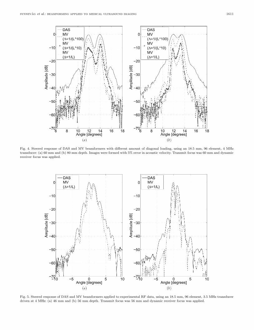
Fig. 4 shows corresponding results for different amountsof diagonal loading. We see that, as the regularization pa-rameter, ∆, increases, the MV amplitude estimates ap-proach those of DAS. As for spatial smoothing, diagonalloading trades off mainlobe width for robustness in theamplitude estimates. Again, the sidelobe level for all ex-amples of ∆ is significantly lower than for DAS.

C. Experimental Data: Wire Targets

We recorded experimental RF data with a specially pro-grammed System FiVe scanner (GE Vingmed Ultrasound,Horten, Norway) using an 18.5 mm, 96 element, 3.5 MHztransducer driven at 4 MHz. The data were sampled at20 MHz and upsampled by a factor 8 before delays were ap-plied. The wires were separated by 2 mm. We used subar-

ray length, L = 48 and ∆ = 1/L for the MV beamformer.Fig. 5 shows the steered responses of the DAS and MVbeamformers at two different depths, for which the latteris at the transmit focal point. We see that the sidelobes aresignificantly lower for the MV beamformer. In Fig. 5(a),which is away from the focal point, the mainlobe width isonly slightly narrower due to the high amount of diagonalloading. At the focal point in Fig. 5(b), the mainlobe widthalso is reduced, demonstrating improved performance onexperimental data.

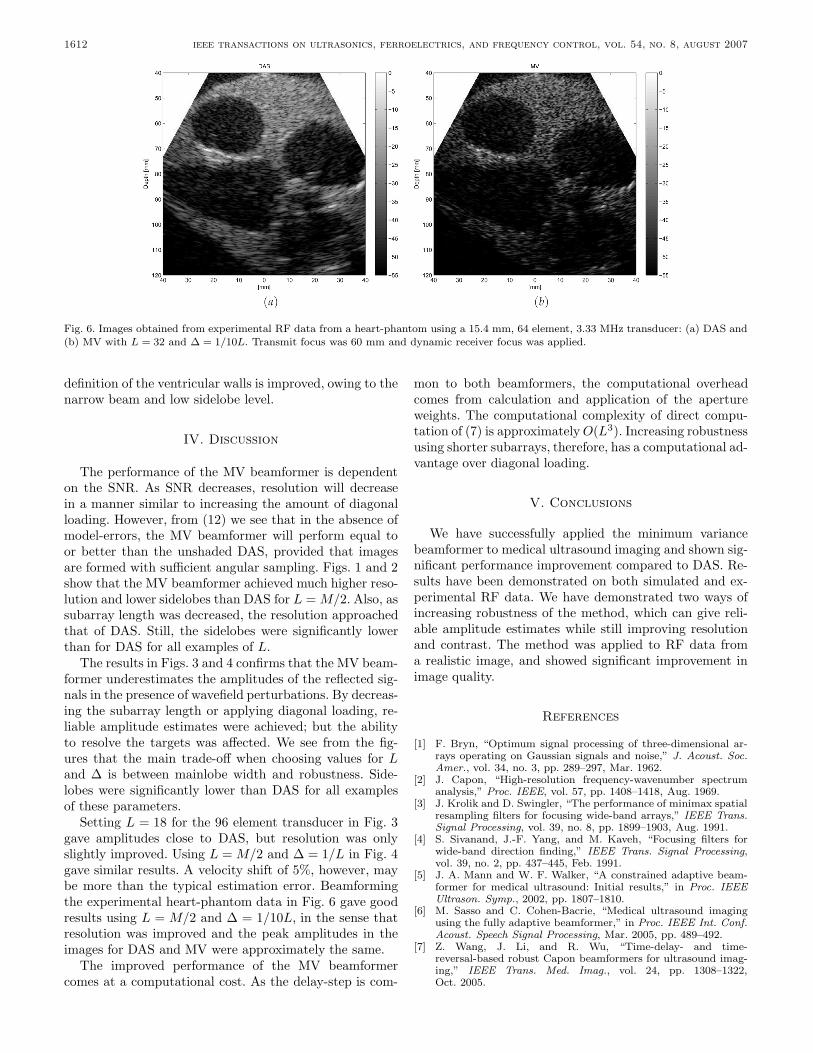
D. Experimental Data: Heart Phantom

The demonstrated properties of the MV beamformer onwire targets should lead to improved contrast and resolu-tion in medical ultrasound images. We applied the methodto experimental RF data from a heart phantom. Thedata-set was obtained from the Biomedical UltrasoundLaboratory, University of Michigan1. Data were recordedwith a 64 element, 3.33 MHz transducer, and sampled at17.76 MHz. Data were upsampled by a factor 8 before de-lays were applied. We used subarray length L = 32, anddiagonal loading with ∆ = 1/10L for the MV beamformer.Transmit focus was 60 mm. Fig. 6 shows the images ob-tained with the DAS and MV beamformers displayed over55 dB dynamic range. We see that the resolution in gen-eral is much better in the MV image. We also see that the

1Ultrasound RF data-set heart from the Biomedical Ultra-sonic Laboratory, University of Michigan, Apr. 2006. Available athttp://bul.eecs.umich.edu/, April 2006.


Fig. 4. Steered response of DAS and MV beamformers with different amount of diagonal loading, using an 18.5 mm, 96 element, 4 MHztransducer: (a) 60 mm and (b) 80 mm depth. Images were formed with 5% error in acoustic velocity. Transmit focus was 60 mm and dynamicreceiver focus was applied.

Fig. 5. Steered response of DAS and MV beamformers applied to experimental RF data, using an 18.5 mm, 96 element, 3.5 MHz transducerdriven at 4 MHz: (a) 46 mm and (b) 56 mm depth. Transmit focus was 56 mm and dynamic receiver focus was applied.


Fig. 6. Images obtained from experimental RF data from a heart-phantom using a 15.4 mm, 64 element, 3.33 MHz transducer: (a) DAS and(b) MV with L = 32 and ∆ = 1/10L. Transmit focus was 60 mm and dynamic receiver focus was applied.

definition of the ventricular walls is improved, owing to thenarrow beam and low sidelobe level.

IV. Discussion

The performance of the MV beamformer is dependenton the SNR. As SNR decreases, resolution will decreasein a manner similar to increasing the amount of diagonalloading. However, from (12) we see that in the absence ofmodel-errors, the MV beamformer will perform equal toor better than the unshaded DAS, provided that imagesare formed with sufficient angular sampling. Figs. 1 and 2show that the MV beamformer achieved much higher reso-lution and lower sidelobes than DAS for L = M/2. Also, assubarray length was decreased, the resolution approachedthat of DAS. Still, the sidelobes were significantly lowerthan for DAS for all examples of L.

The results in Figs. 3 and 4 confirms that the MV beam-former underestimates the amplitudes of the reflected sig-nals in the presence of wavefield perturbations. By decreas-ing the subarray length or applying diagonal loading, re-liable amplitude estimates were achieved; but the abilityto resolve the targets was affected. We see from the fig-ures that the main trade-off when choosing values for Land ∆ is between mainlobe width and robustness. Side-lobes were significantly lower than DAS for all examplesof these parameters.

Setting L = 18 for the 96 element transducer in Fig. 3gave amplitudes close to DAS, but resolution was onlyslightly improved. Using L = M/2 and ∆ = 1/L in Fig. 4gave similar results. A velocity shift of 5%, however, maybe more than the typical estimation error. Beamformingthe experimental heart-phantom data in Fig. 6 gave goodresults using L = M/2 and ∆ = 1/10L, in the sense thatresolution was improved and the peak amplitudes in theimages for DAS and MV were approximately the same.

The improved performance of the MV beamformercomes at a computational cost. As the delay-step is com-

mon to both beamformers, the computational overheadcomes from calculation and application of the apertureweights. The computational complexity of direct compu-tation of (7) is approximately O(L3). Increasing robustnessusing shorter subarrays, therefore, has a computational ad-vantage over diagonal loading.

V. Conclusions

We have successfully applied the minimum variancebeamformer to medical ultrasound imaging and shown sig-nificant performance improvement compared to DAS. Re-sults have been demonstrated on both simulated and ex-perimental RF data. We have demonstrated two ways ofincreasing robustness of the method, which can give reli-able amplitude estimates while still improving resolutionand contrast. The method was applied to RF data froma realistic image, and showed significant improvement inimage quality.

References

[1] F. Bryn, “Optimum signal processing of three-dimensional ar-rays operating on Gaussian signals and noise,” J. Acoust. Soc.Amer., vol. 34, no. 3, pp. 289–297, Mar. 1962.

[2] J. Capon, “High-resolution frequency-wavenumber spectrumanalysis,” Proc. IEEE, vol. 57, pp. 1408–1418, Aug. 1969.

[3] J. Krolik and D. Swingler, “The performance of minimax spatialresampling filters for focusing wide-band arrays,” IEEE Trans.Signal Processing, vol. 39, no. 8, pp. 1899–1903, Aug. 1991.

[4] S. Sivanand, J.-F. Yang, and M. Kaveh, “Focusing filters forwide-band direction finding,” IEEE Trans. Signal Processing,vol. 39, no. 2, pp. 437–445, Feb. 1991.

[5] J. A. Mann and W. F. Walker, “A constrained adaptive beam-former for medical ultrasound: Initial results,” in Proc. IEEEUltrason. Symp., 2002, pp. 1807–1810.

[6] M. Sasso and C. Cohen-Bacrie, “Medical ultrasound imagingusing the fully adaptive beamformer,” in Proc. IEEE Int. Conf.Acoust. Speech Signal Processing, Mar. 2005, pp. 489–492.

[7] Z. Wang, J. Li, and R. Wu, “Time-delay- and time-reversal-based robust Capon beamformers for ultrasound imag-ing,” IEEE Trans. Med. Imag., vol. 24, pp. 1308–1322,Oct. 2005.


[8] J.-F. Synnevag, A. Austeng, and S. Holm, “Minimum vari-ance adaptive beamforming applied to medical ultrasound imag-ing,” in Proc. IEEE Ultrason. Symp., 2005, pp. 1199–1202.

[9] F. Viola and W. F. Walker, “Adaptive signal processing in med-ical ultrasound beamforming,” in Proc. IEEE Ultrason. Symp.,2005, pp. 1980–1983.

[10] T.-J. Shan, M. Wax, and T. Kailath, “On spatial smoothing fordirection-of-arrival estimation of coherent signals,” IEEE Trans.Acoust. Speech Signal Processing, vol. 33, no. 4, pp. 806–811,Aug. 1985.

[11] P. Stoica and R. Moses, Introduction to Spectral Analysis. En-glewood Cliffs, NJ: Prentice-Hall, 1997.

[12] J. Li, P. Stoica, and Z. Wang, “On robust Capon beamformingand diagonal loading,” IEEE Trans. Signal Processing, vol. 51,no. 7, pp. 1702–1715, July 2003.

[13] A. Ozbek, “Adaptive seismic noise and interference attenuationmethod,” U.S. Patent No.: US 6,446,008 B1, Sep. 2002.

[14] J. A. Jensen, “Field: A program for simulating ultrasound sys-tems,” Med. Biol. Eng. Comput., vol. 34, pp. 351–353, 1996.

[15] B. A. J. Angelsen, Ultrasound Imaging. Waves, Signals and Sig-nal Processing. Trondheim, Norway: Emantec, 2000.

Johan-Fredrik Synnevag (S’06) was bornin Bergen, Norway, in 1974. He received theM.S. degree in computer science from the Uni-versity of Oslo, Oslo, Norway, in 1998. From1999 to 2004 he worked as a project engineerin Schlumberger (now WesternGeco), Asker,Norway. He is currently pursuing a Ph.D. de-gree in signal processing at the University ofOslo.

His research interests include array signalprocessing.

Andreas Austeng (S’97–M’02) was born inOslo, Norway, in 1970. He received the M.S.degree in physics in 1996 and the Ph.D. de-gree in computer science in 2001, both fromthe University of Oslo, Oslo, Norway. Since2001 he has been working at the Departmenton Informatics, University of Oslo, first as apostdoctoral research fellow, and currently asan associate professor.

His research interests include signal pro-cessing for acoustical imaging.

Sverre Holm (M’82–SM’02) was born inOslo, Norway, in 1954. He received the M.S.and Ph.D. degrees in electrical engineeringfrom the Norwegian Institute of Technology,Trondheim, in 1978 and 1982.

He has done research and developmentin speech coding and frequency estimationat SINTEF, Trondheim, Norway, and workedwith synthetic aperture radar processing andspectral estimation at InformasjonskontrollAS, Asker, Norway. From 1990 to 1994 he wasat GE Vingmed Ultrasound, Horten, Norway,

doing research and development work in digital beamforming, ultra-sound probes, and ultrasound contrast agents. He spent the fall of1998 on a sabbatical at GE Global Research, Schenectady, NY.

He has been an assistant professor in the Electrical EngineeringDepartment of Yarmouk University in Jordan (1984–1986) and from1989 he was an adjunct professor, until 1992 at the Norwegian In-stitute of Technology, then at the University of Oslo, Oslo, Norway.Since 1995 he has been a full professor of signal processing at theUniversity of Oslo working in ultrasound and sonar imaging, acous-tic field simulation, and indoor positioning systems.

Dr. Holm was an associate editor of the IEEE Transactions onUltrasonics, Ferroelectrics, and Frequency Control from 1997–2002.He was elected as a member of the Norwegian Academy of Techno-logical Sciences in 2002.

Adaptive Beamforming Applied to Medical Ultrasound · PDF file1606 ieee transactions on...

Documents

Transcript of Adaptive Beamforming Applied to Medical Ultrasound · PDF file1606 ieee transactions on...