Adaptive Disk Spindown via Optimal Rent-to-Buy inProbabilistic Environments�P. KrishnanyAT&T Bell Laboratories101 Crawfords Corner RoadP. O. Box 3030Holmdel, NJ 07733pk@research.att.comPhilip M. LongzDept. of Computer ScienceDuke UniversityP. O. Box 90129Durham, NC 27708plong@cs.duke.edu

Je�rey Scott VitterxDept. of Computer ScienceDuke UniversityP. O. Box 90129Durham, NC 27708jsv@cs.duke.eduAbstractIn the single rent-to-buy decision problem, without a priori knowledge of the amount of timea resource will be used we need to decide when to buy the resource, given that we can rent theresource for $1 per unit time or buy it once and for all for $c. In this paper we study algorithmsthat make a sequence of single rent-to-buy decisions, using the assumption that the resource usetimes are independently drawn from an unknown probability distribution. Our study of this rent-to-buy problem is motivated by important systems applications, speci�cally, problems arisingfrom deciding when to spindown disks to conserve energy in mobile computers [DKM, LKH,MDK], thread blocking decisions during lock acquisition in multiprocessor applications [KLM],and virtual circuit holding times in IP-over-ATM networks [KLP, SaK].We develop a provably optimal and computationally e�cient algorithm for the rent-to-buyproblem. Our algorithm uses O(pt) time and space, and its expected cost for the tth resource useconverges to optimal as O(plog t=t), for any bounded probability distribution on the resourceuse times. Alternatively, using O(1) time and space, the algorithm almost converges to optimal.We describe the experimental results for the application of our algorithm to one of themotivating systems problems: the question of when to spindown a disk to save power in a mobilecomputer. Simulations using disk access traces obtained from an HP workstation environmentsuggest that our algorithm yields signi�cantly improved power/response time performance overthe non-adaptive 2-competitive algorithm which is optimal in the worst-case competitive analysismodel.�An extended abstract appears in the Twelfth International Machine Learning Conference, July 1995.ySupport was provided in part by an IBM Fellowship, by NSF research grant CCR{9007851, by Army ResearchO�ce grant DAAH04{93{G{0076, and by Air Force O�ce of Scienti�c Research grant F49620{94{1{0217. This workwas done while the author was visiting Duke University from Brown University.zSupported in part by Air Force O�ce of Scienti�c Research grants F49620{92{J{0515 and F49620{94{1{0217.xSupported in part by National Science Foundation research grant CCR{9007851, by Air Force O�ce of Scienti�cResearch grants F49620{92{J{0515 and F49620{94{1{0217 and by a Universities Space Research Association/CESDISassociate membership.

1 IntroductionThe single rent-to-buy decision problem can be described as follows: we need a resource for anunknown amount of time, and we have the option to rent it for $1 per unit time, or to buy it onceand for all for $c. For how long do we rent the resource before buying it? The best algorithmwith full prior knowledge of how long the resource will be needed (an o�ine algorithm) will buythe resource immediately if the resource will be needed for at least c time units and rent otherwise.An online algorithm (i.e., one without a priori knowledge of how long the resource will be needed)that rents the resource for c units of time and then buys it incurs a cost of at most 2 times the costof the best o�ine algorithm. This competitive factor1 of 2 is the best possible (for deterministicalgorithms) in the worst case [KMM]. If we know of a probability distribution on the time theresource is needed, we can usually �nd a rent-to-buy strategy whose expected cost is substantiallyless than that of the online algorithm that waits c time units before buying.In this paper we are interested in the rent-to-buy problem described above with two importantadditional features motivated by practical applications. Many interesting systems problems canbe modeled well by a sequence of single rent-to-buy problems. To solve the tth single rent-to-buyproblem (or the tth round), the online algorithm can use what it has learned from the previoust�1 rounds. (The online algorithm that waits for c time before buying in each round is still withina factor of 2 of the best possible.) We call this the sequential rent-to-buy problem, or just the rent-to-buy problem. In these real-life situations we can assume that the time for which the resourceis needed in each round is drawn from a probability distribution. However, it is unreasonable toassume that the distribution is known a priori. We now describe three interesting problems modeledby a sequence of rent-to-buy decisions.The Disk Spindown Problem. Energy conservation is an important issue in mobile computing.Portable computers run on battery power and can function for only a few hours before drainingtheir batteries. Current techniques for conserving energy are based on shutting down componentsof the system after reasonably long periods of inactivity. Recent studies show that the disk sub-system on notebook computers is a major consumer of energy [DKM, LKH, MDK]. Most disksused for portable computers (e.g., the small, light-weight Kittyhawk from Hewlett Packard [Pac])have multiple energy states. Conceptually, the disk can be thought of as having two states: thespinning state in which the disk can access data but consumes a lot of energy and a spundownstate in which the disk consumes e�ectively no energy but cannot access data.2 Spinning down adisk and spinning it up consumes a �xed amount of energy and time (and also produces wear andtear on the disk). During periods of inactivity, the disk can be spundown to conserve energy at theexpense of increased latency for the next request. The disk spindown problem is to decide when tospindown the disk so as to conserve energy, with acceptable latency.The disk spindown scenario can be modeled as a rent-to-buy problem as follows. A round isthe time between any two requests for data on the disk. For each round, we need to solve the diskspindown problem. Keeping the disk spinning is viewed as renting, since energy is continuouslyexpended to keep the disk spinning. Spinning down the disk is viewed as a buy, since the energyto spindown the disk and spin it back up upon the next request is independent of the remainingamount of time until the next disk access. The cost of the increased latency in serving the nextdisk access can also be integrated into the cost of the buy, if the algorithm is given as an input the1A k-competitive algorithm incurs a cost of at most O(1) plus k times the cost of the optimal o�ine algorithm.2In general, the disks provide more than just two power management states, but only one state, the fully spinningstate, allows access to data. 1

relative importance of conserving energy and responding quickly to disk accesses. (This is discussedin detail in Section 6.) Based on observations of disk access patterns in workstation environments[RuW], the times between accesses to disk (which de�ne the rounds) can be assumed to be generatedby a probability distribution. The disk spindown problem will be our main motivating applicationfor this study.The Spin/Block Problem. Another interesting and important problem from multiprocessorapplications, the spin/block problem, involves threads trying to acquire locks to protect access toshared data [KLM]. A round is de�ned by a thread requesting locked data and eventually acquiringthe lock. In a round, the system can have the thread wait (or spin) until the lock is free, incurringa �xed cost per unit time for wasted processor cycles, or block and incur a higher context switchoverhead. The spinning can thus be viewed as renting, and a block can be viewed as a buy. Inthis situation too, practical studies suggest that lock-waiting times can be assumed to obey someunknown but time-invariant probability distribution [KLM].The Virtual Circuit Problem. Deciding virtual circuit holding times in IP-over-ATM networksis another scenario modeled by the rent-to-buy framework [SaK]. When carrying Internet protocol(IP) tra�c over an Asynchronous Transfer Mode (ATM) network, a virtual circuit is opened uponthe arrival of an IP datagram, and the ATM adaptation layer has to decide how long to hold avirtual circuit open. There are many possible pricing policies for virtual circuit holding times. Asdescribed in [SaK, Section 5], in future ATM networks, it is expected that a large number of virtualcircuits could be held open by paying a charge per unit time to keep the circuit open. Keeping thevirtual circuit open can be thought of as a \rent" while closing it can be considered a \buy." Theinter-arrival time of packets on a circuit (i.e., the resource use times in the rent-to-buy model) canbe modeled as being drawn independently from a probability distribution [LPR, SaK].An algorithm for the sequential rent-to-buy problem can be visualized in two ways. In anyround, the algorithm can be thought of as making sequential binary decisions of \should I buynow?" Alternatively, we can think of the algorithm as setting a threshold or cuto� on the costit is willing to accrue before buying, and behaving according to the cuto�. These two views aretrivially equivalent; we adopt the second for convenience. There are two important requirements ofany good online algorithm for the rent-to-buy problem: the algorithm should produce good cuto�s,and it should use minimal space and time to output its cuto�s. In this paper we develop onlinealgorithms for the rent-to-buy problem in probabilistic environments, assuming that the resourceuse times are independently randomly drawn from a �xed but unknown probability distribution.The most straightforward solution to the problem [KMM] is to store all past resource use times,and use that cuto� b for the current round which would have had the lowest total cost had we usedit in the past. Straightforward application of results of Vapnik [Vap] implies that the expected rent-to-buy cost of this strategy converges to that of the best �xed cuto�. One can easily see that thecuto� b at any given time falls on (actually, near) one of the past resource use times; however, eventaking this into account, this solution is computationally expensive. For the tth round, this solutionwould need space and time proportional to O(t), and this is unacceptable in system environments.In this paper, we develop an algorithm L for the rent-to-buy problem which, for arbitrary prob-ability distributions with support on [0;M ], converges to optimal; i.e., the cost of the algorithmconverges to the cost of the best algorithm with full prior knowledge of the distribution. More im-portantly, for the tth round that lasts xt time, the algorithm uses O(cpt) space, generates its cuto�sin O(1) time, and uses O((minfxt; cg)pt+log(ct)) time to update its data structures. Alternatively,our algorithm can be adapted to work in a situation when the space it can use is limited. Presented2

with O(s) space, our algorithm Ls uses O(1) time to generate cuto�s, O((minfxt; cg)s + log(cs))time to update its structures, and almost converges to optimal, being away from optimal additivelyby O(minfM; cg=s). The O(xt) component of the time used in updating the data structure can bedone \on the y" as the round is progressing. For example, in the disk spindown scenario, let thetth idle time at disk be z < c seconds. Before the idle period starts, algorithm Ls outputs its rec-ommended spindown threshold using O(1) time, and updates its data structure in O(zs+ log(ct))time. The updates corresponding to the \zs" term can be done while the disk is waiting for thenext access.Most practical situations are well-modeled by bounded distributions. For example, in the diskspindown scenario, any reasonable algorithm will spin down the disk after a few minutes (say,30 minutes) since the last access. Therefore, all idle times at disk greater than 30 minutes arepractically equivalent, and can be assumed to be 30 minutes without loss of generality, resulting ina distribution with bounded support.Simulations of our algorithm on disk access traces obtained from HP show that by giving asuitable value of c to our algorithm, we e�ectively trade power for response time (latency). InSection 6 we introduce the natural notions of excess energy and e�ective cost. The \excess energy"discounts from the total energy the portion that every algorithm would have to spend; the e�ectivecost is a measure that merges the e�ects of energy conservation and response time performanceinto one metric based on a user speci�ed parameter a, the relative importance of response timeto energy conservation. (The buy cost c varies linearly with a.) We show that our algorithm L isbest amongst the online algorithms considered in terms of e�ective cost for almost all values of a,saving e�ective cost by 6{25% over the optimal online algorithm in the competitive model (i.e.,the 2-competitive algorithm that spins down the disk after waiting c seconds). In addition, forsmall values of a (corresponding to when saving energy is critical), our algorithm when comparedagainst the 2-competitive algorithm reduces excess energy by 17{60%, and when compared againstthe 5 second threshold, it reduced excess energy by 6{42%.1.1 Related WorkThe single rent-to-buy problem has been studied in the worst-case setting and e�cient deterministicand randomized algorithms have been developed for the problem by Karlin et al. [KMM]. In partic-ular, 2-competitive deterministic algorithms and e=(e�1)-competitive randomized algorithms havebeen developed. In [KMM] it was claimed that there is an adaptive algorithm achieving a com-petitive ratio approaching e=(e � 1) on input sequences generated according to any time invariantprobability distribution. However, their technique as stated is computationally ine�cient.For the disk spindown problem, current mobile computers spin disks down after about �veminutes of inactivity. In [DKM, LKH], the authors propose a more aggressive spindown policy,and support their proposal by simulation studies on workstation and notebook traces. The studiessuggest that the gain in energy often overshadows the loss in response time. In [DKM], the com-parison of �xed-threshold strategies is made against optimal o�ine algorithms. The authors alsomention trying out predictive disk spindown policies. Adaptive spindown policies that continuallychange the spindown threshold based on perceived inconvenience to the user are studied in [DKB].In [Gre], Greenawalt looks at the disk spindown problem assuming a Poisson arrival of requests atdisk, and studies disk spindown and reliability issues.Karlin et al. in [KLM] have studied the spin/block problem empirically, evaluating di�erentspin/block strategies including �xed-threshold and adaptive strategies. The virtual circuit problemhas been empirically studied by Saran et al. [SaK], where they propose a Least Recently Used3

(LRU)-based holding time policy as performing well in their studies. The �rst LRU-based holdingtime policy they study is the 2-competitive algorithm described earlier in this paper, and theirsecond holding time policy involves estimating the mean inter-reference interval with exponentialaveraging. In [KLP], Keshav et al. empirically study an adaptive policy for the virtual circuitproblem that tries to estimate the distribution of inter-arrival times by keeping a histogram ofobserved inter-arrival times grouped into �xed size buckets.In Section 2, we describe the main analytical results of the paper. We present algorithm A�in Section 3; algorithm A� lies at the heart of our optimal rent-to-buy algorithms, L and Ls.We analyze algorithm A� for space used, computational time, and convergence rate in Section 4.We describe how algorithm A� can be used to get algorithms L, Ls in Section 5. We explain inSection 6 precisely how the disk spindown problem can be modeled in the rent-to-buy framework,when the user is concerned about energy conservation and response time performance. We presentour experimental results in Section 7 and conclude in Section 8.2 De�nitions and Main Analytical ResultsWe denote the reals by IR, the nonnegative reals by IR+, and the positive integers by IN. An onlinerent-to-buy algorithm is given the relative cost c � 1 of buying. It works in rounds, where in thetth round, it �rst formulates a cuto� on the amount of time it will wait before buying, and thengets the tth resource use time. A rent-to-buy algorithm de�nes a mapping from [n2IN(IR+)n (thepast resource use times) to IR+ (the cuto� generated). In other words, A(x1; x2; : : : ; xt) is thecuto� generated by algorithm A in the (t+ 1)st round, when the previous resource use times werex1; x2; : : : ; xt. If the resource use time in any round is x, then the cost of choosing cuto� b iscostc(x; b) = ( x if x � bb+ c otherwise.For the disk spindown problem, the resource use time in round t corresponds to the tth idle timeat disk, and a cuto� is a spindown threshold.Our �rst main result is an algorithm L that approaches optimal and is e�cient in terms of thespace and time it uses.Theorem 1 For any c > 1, M > 1, there is a rent-to-buy algorithm L that on round t with resourceuse time xt,� uses O(cpt) space� outputs its choice of cuto� in O(1) time, and updates its data structures in O((minfxt; cg)pt+log(ct)) time, and� incurs a cost that approaches optimal: there exists k such that for any distribution D on[0;M ], for all large enough t 2 IN,E~x2Dt(costc(xt; L(x1; :::; xt�1))) � infa Ez2D(costc(z; a)) + ks ln tt :Note that in Theorem 1, the same k can used for any distribution with support on [0;M ].Further, the time and space bounds are independent of D as well. It is easy to adapt algorithm L4

to get algorithm L0 that successively increases its estimate of M , and converges to optimal for anydistribution. However, the convergence rate of algorithm L0 would depend on the distribution.In many practical situations, we would like to �x the amount of space and time used by our algo-rithm while converging approximately, rather than exactly, to optimal. Algorithm Ls, a restrictedspace version of Algorithm L, can be used in this scenario.Theorem 2 When presented with s > k ln2(M+c) ln ln(M+c) bytes of space, where k is a constantindependent of M and c, for the tth round, algorithm Ls outputs its choice of cuto� in O(1) time,updates its data structures in O((minfxt; cg)s + log(cs)) time, and for any probability distributionD on [0;M ] for all large enough t 2 IN, converges approximately to optimal:E~x2Dt(costc(xt; Ls(x1; :::; xt�1))) � infa Ez2D(costc(z; a)) +O�minfc;Mgs � :We simulated our algorithms for the disk spindown problem using disk access traces obtainedfrom an HP workstation environment. Our simulation results are described in Section 7.One obvious approach to attack the rent-to-buy problem in probabilistic environments is to learnthe distribution on times for the rounds, calculate the optimal cuto� for the estimated distribution,and output that cuto� for each round. This is unacceptable from the computational standpoint.In our algorithms, we bypass the estimation of the distribution, directly estimating the e�cacy ofdi�erent cuto� points. The analysis is complicated, however, by the fact that there are in�nitelymany cuto� points to evaluate at any given time on the basis of a �nite number of samples fromthe distribution. We show for the rent-to-buy problem that to get a good solution, it is su�cientto consider a small �nite set of possible cuto� points. The appropriate choice of this set dependson the distribution, and is done using the information gained in early rounds. We call this basicstrategy that chooses the appropriate set of possible cuto�s and evaluates them to determine thebest cuto� to use in any round as algorithm A�.Our algorithm L is based on algorithm A�. It chooses from among successively larger �nitesets of possible cuto� points to converge to optimal. A tree data structure, which is modi�eddynamically, is used to store the estimated quality of each considered cuto� point. Algorithm Lssets appropriate parameters based on the available space s, and uses algorithm A� to convergeapproximately to optimal.We �rst describe algorithm A� which lies at the heart of our optimal algorithms L and Ls.3 The Main Idea: Algorithm A�Algorithm A� takes as parameters � and M , and attempts to achieve an expected cost on a givenround which is at most � greater than the expected cost incurred by the optimal cuto�. We willalso call a resource use time an \example." Our algorithms estimate optimal cuto�s based on pastresource use times; in other words, they estimate optimal cuto�s based on the examples they haveseen.Algorithm A� works in two stages. In the �rst stage, it uses a small number of examples togenerate a small number of candidate cuto�s. (For the small number of rounds that constitutethe �rst stage, the algorithm chooses an arbitrary cuto�, say buying immediately.) It �xes thesecandidate cuto�s and then starts its second stage. For the tth round in the second stage, itevaluates the candidate cuto�s on the past t� 1 examples, and chooses the cuto� with minimumtotal cost. The important point is that these small number of candidate cuto�s when generated5

carefully are su�cient to achieve a small enough cost, as described in Section 4.2. Also, updatingthese cuto�s can be done e�ciently, as described in Section 4.3. We call an � such that 0 < � <1=(ln2(M + c) ln ln(M + c)) a suitable epsilon; for technical reasons, we assume in our discussionsthat � is suitable.Note that the problem is trivial if c �M , since no reasonable algorithm would ever buy in thiscase; the case of interest is when c�M .3.1 First StageIn the �rst stage, algorithm A� generates candidate cuto�s b0; b1; : : : ; bv by partitioning [0;M ] intov intervals. Intuitively, to be accurate in its estimations in the second phase, algorithm A� wantsthese candidate cuto�s to be close in one of two senses: either that the probability of a point fallingbetween them is not too large, or in absolute distance. However, for computational e�ciency, wedo not want too many candidate cuto�s. Hence, algorithm A� attempts to partition [0;M ] intov � d4c=�e intervals, such that1. each interval is at least �=2 in length, and2. if an interval has length > �=2, then the interior of the interval has probability at most �=2c.The endpoints of the intervals de�ne the candidate cuto�s.We say that an interval satis�es the computational criterion if it is at least �=2 in length, and thatit satis�es the density criterion if the probability of the interval is at most �=2c. (In other words,at the end of the �rst stage, algorithm A� ensures that every interval satis�es the computationalcriterion, and intervals of length greater than �=2 satisfy the density criterion.) Conceptually, wecan think of algorithm A� as generating v0 intervals that each satisfy the density criterion, andthen moving the potential cuto�s apart (discarding intervals of size 0) to get v � v0 intervals suchthat the computational criterion holds for each interval. As a result of the VC theory [BEH, VaC],it is easy to partition [0;M ] into v intervals satisfying the density criterion with high probability,by storing � = �(v ln v) examples, and calling a procedure generate cutoffs(w; �; �) on [0;M ].The procedure generate cutoffs breaks a speci�ed interval into w intervals by taking a set �of � examples, and ensuring that in any interval we have �=w examples from �. (The proceduregenerate cutoffs can be implemented by sorting � to get � and iteratively moving through �=wexamples in � to de�ne the intervals.)Algorithm A� implements its �rst stage in a space e�cient manner by storing at most O(v)examples at any time. It performs the �rst stage in three phases. In the �rst phase, algorithm A�partitions [0;M ] \roughly" into B big intervals, and in the second phase it re�nes these big in-tervals one by one into approximately v0=B intervals each. While re�ning a speci�c big interval,algorithm A� discards examples that do not fall in the big interval. In the third phase, algorithm A�moves potential candidate cuto�s apart to ensure that the computational criterion is met.Formally, algorithm A� works as follows. Let � = �=(4(c +M)), and let the array � storethe examples being retained by algorithm A�. In the �rst phase, it divides the interval [0;M ]into B = k ln(1=�)=2 big intervals (where k is a constant independent of �, M , and is asde�ned in Lemma 2). It does this by collecting �1 = 4kB ln(2B=�) examples and callinggenerate cutoffs(B; �1; �) on interval [0;M ]. The second phase consists of B subphases, wherein the ith subphase, algorithm A� divides the ith big interval into d4c=(B�)e intervals. It doesthis by sampling at most �02 = 4B(�2 + ln(2B=�)) examples, where �2 = 4kc ln(4c=(��))=(�B), andstoring the �rst �2 examples that fall within the ith big interval. Let �2;i � �2 be the number6

of examples stored in the ith subphase. Algorithm A� calls generate cutoffs(d4c=(B�)e; �2;i; �)on the ith big interval. (We will see in Section 4.1 that �2;i = �2 with high probability.) At theend of the second phase, we are left with the required v0 � d4c=�e intervals. In the third phase,algorithm A� ensures that the computational criterion is met. Let the ith interval at the end of thesecond phase be [l0i; r0i). Algorithm A� sets l0 = 0, r0 = max(�=2; r00), and processes the intervalsiteratively by setting li = ri�1, and ri = max(r0i; li + �=2). The ith interval is de�ned to be [li; ri),and intervals such that li = ri are discarded. The total number of resulting intervals is v � d4c=�e.The candidate cuto�s are de�ned to be bi = li, 0 � i < v, bv =M .3.2 Second stageIn the second stage, algorithm A� repeatedly chooses the cuto� from among those in fb0; b1; :::; bvgthat performed the best in the past. Formally, it formulates its tth cuto� in the second stage asfollows. If x1; x2; :::; xt�1 are the resource use times previously seen in the second stage, for alli 2 IN; 0 � i � v, algorithm A� sets qi = t�1Xj=1 costc(xj ; bi):It uses a bi for which qi � qk for all k 2 f0; :::; vg as its cuto� for the tth round.We now study the performance of algorithm A� in terms of space used, the convergence rate,and time required for updates.4 Goodness of Algorithm A�In Section 4.1, we see that algorithm A� can be implemented with O(v) space, and generates goodcuto�s with high probability. In Section 4.2 we see that the distance algorithm A� is away fromoptimal approaches � as t gets large, and in Section 4.3 we see that in the second stage the strategiescan be updated e�ciently with a tree-based data structure.4.1 Guarantees about the First StageLet � = �=(4(c +M)), B = k ln(1=�)=2, �1 = 4kB ln(2B=�), and �2 = 4kc ln(4c=(��))=(�B) beas de�ned in Section 3.1. From the discussion in Section 3.1, it follows that the space used byAlgorithm A� in the �rst stage is bounded by the number of examples we use at any time plus thenumber of cuto�s we retain; i.e., the space used is bounded by B+v+maxf�1; �2g = O(v) = O(c=�).The operations in the third phase of the �rst stage ensure that every interval satis�es thecomputational criterion. We say that the �rst stage fails if at the end of the �rst stage there isan interval of length greater than �=2 not satisfying the density criterion. The event that the �rststage fails is a subset of the event that at the end of the second phase, there is some interval thatdoes not satisfy the density criterion.Let `� be the total number of examples we see in the �rst stage; i.e., all examples, including theones we discard. We now see that the �rst stage fails with low probability (i.e., probability 2�).Lemma 1 Let `� = lkc ln2 ((c+M)=�) =�m be the number of examples seen in the �rst stage (wherek is as de�ned in Lemma 2), let � = �=(4(c+M)), and let E1 be the event that the �rst stage fails.Then, for any � that is suitable, Pr(E1) � �=(2(c +M)).7

To prove the above lemma, we use a technique due to Kearns and Schapire [KeS]. Lemma 2below follows immediately from the results of Blumer et al. [BEH] using the techniques of Vapnikand Chervonenkis [VaC]. Informally, Lemma 2 says that m points are enough to simultaneouslyestimate the probabilities of every interval.Lemma 2 Choose 0 < �; � � 1=2; c � 1; and a probability distribution D on IR+. Then thereexists k > 0 such that if m = l k�(ln 1� + ln 1� )m thenPr~x2Dm �9a; b s.t. PrD((a; b)) � 2� and 1m jfj : xj 2 (a; b)gj � �� � �and Pr~x2Dm �9a; b s.t. PrD((a; b)) � �=2 and 1m jfj : xj 2 (a; b)gj � �� � �:The standard Cherno� bounds will be helpful to prove Lemma 1.Lemma 3 (Cherno�) For t independent Bernoulli trials each of which has a probability of successat least p, let LE(p; t; r) denote the probability that there are at most r successes in the t trials.Then, for 0 < p < 1, and 0 � q � p,LE(p; t; qt) � e�(p�q)2t=2pProof of Lemma 1: The value for `� was obtained by assuming that the �rst phase requiresus to look at �1 = 4kB ln(2B=�) examples, and the ith subphase of the second phase requiresus to look at a total of �02 = 4B(�2 + ln(2B=�)) examples, where �2 = 4kc ln(4c=(��))=(�B), andB = k ln(1=�)=2. We bound the probability of the �rst stage failing by the probability of the eventthat at the end of the second phase there is some interval that does not satisfy the density criterion.We say that the �rst phase fails, if any big interval generated in the �rst phase has probabilitygreater than 2=B or less than 1=2B. We say that the ith subphase fails if any interval generatedin the ith subphase has probability greater than �=2c; the second phase fails if for any i, the ithsubphase fails. The lemma is proved if we can bound the probability of the �rst phase failing or anyof the subphases failing by �=B, since the net failure probability is then bounded by (�=B)�(B+1) ��=(2(c +M)).From Lemma 2, by setting � = 1=B and � = �=(2B), we can easily verify that if we look at �1examples, the �rst phase fails with probability at most �=B. We now assume that the �rst phasedid not fail; i.e., the probability of any big interval is between 1=2B and 2=B. We could fail inthe ith subphase if we either do not get �2 examples in the ith big interval, or if after using the �2examples we get an interval with probability > �=2c. From Lemma 3, by substituting p = 1=(2B),r = �2, and t = �02, we see that the probability that the number of examples that fall in the ith biginterval is less than �2 is at most �=(2B). From Lemma 2, by setting � = �B=(4c) and � = �=(2B),we see that the probability that the �2 examples did not divide the ith big interval into subintervalswith probability � �=2c is at most �=2B. Hence the probability of the ith subphase failing is atmost �=B. 24.2 Convergence of Algorithm A�We have seen that the �rst stage works with high probability. The main result of this subsectionis to bound the performance of A�. 8

Theorem 3 Choose M , c such that M > c � 1. Choose any � that is suitable, and let m =lkc ln2 ((c+M)=�) =�m be the number of examples seen by algorithm A� in the �rst stage, wherek is de�ned as in Lemma 2. There exists k1 > 0 such that for su�ciently large t 2 IN, for anydistribution D on [0;M ],E(~u;~x)2Dm�Dt(costc(xt; A�(u1; :::; um; x1; :::; xt�1)))� (infaEz2D(costc(z; a))) + �+ k1(c+M)r ln ((c+M)t=�)t :To prove the above theorem, we �rst show that if the �rst stage was successful, then one of thepossible cuto�s bj generated in the �rst stage is only �=2 away from optimal (Lemma 4). Intuitively,by choosing the cuto� with minimal cost in the second stage, we are close to bj in cost. We thenbound the error in expected cost resulting from the �rst stage failing and prove Theorem 3.Lemma 4 Choose 0 < � � 1=2, c � 1, s 2 IN, and a probability distribution D on [0;M ]. Choose0 = b0 < b1 < ::: < bs =M: If for all j 2 f1; :::; sg, either PrD((bj�1; bj)) � �=2c, or bj�bj�1 = �=2,then there exists i� 2 f0; :::; sg such thatEz2D(costc(z; bi�)) � infa Ez2D(costc(z; a)) + �2 :Proof : Intuitively, if the optimal cuto� lies between bj�1 and bj , the way in which the candidatecuto�s were chosen ensures that the interval (bj�1; bj) is \small enough" (in probability or absolutesize) so that one of bj�1 or bj is close to optimal.Assume without loss of generality that no bi is exactly optimal; i.e., for all � > 0, there existsan a� 62 fb0; :::; bsg, such that costc(z; a�) = infaEz2D(costc(z; a)) + �. Choose � > 0 and �x a�,bj�1 < a� < bj. We now show that one of i� = j � 1 or i� = j satis�es the lemma.Case 1. Pr(bj�1; bj) � �=2c. In this case, we show that the lemma holds with i� = j � 1. If aresource use time z lies outside of the interval [bj�1; a�), then the cuto� a� incurs at least as muchcost as the cuto� bj�1, since a� > bj�1. If the resource use time z 2 (bj�1; a�], then the expectedextra cost of cuto� bj�1 is at most c �PrD((bj�1; a�)) � c � (�=2c) � �=2.Ez2D(costc(z; bj�1)) � Ez2D(costc(z; a�) j z 62 [bj�1; a�)) �Prz2D(z 62 [bj�1; a�))+Ez2D(costc(z; a�) + c j z 2 (bj�1; a�]) �PrD((bj�1; a�])� Ez2D(costc(z; a�)) + �=2 (since PrD((bj�1; bj)) � �=2c)� infa Ez2D(costc(z; a)) + � + �=2:Case 2. Pr(bj�1; bj) > �=2c. In this case, we show that the lemma holds with i� = j. Note thatbj � bj�1 = �=2. For all c > 1 and all distributions D, Ez2D(costc(z; a)) viewed as a function of ais Lipschitz bounded in one direction in a sense. (This is in spite of the fact that this function of ahas jump discontinuities in general.) That is, if 0 � a1 < a2, thenEz2D(costc(z; a2))�Ez2D(costc(z; a1)) � a2 � a1:Hence, Ez2D(costc(z; bj))�Ez2D(costc(z; a�)) � bj � a� � bj � bj�1 � �2 ;9

which implies that Ez2D(costc(z; bj�1)) � infa Ez2D(costc(z; a)) + � + �=2:Since � > 0 was chosen arbitrarily, this completes the proof. 2The standard Hoe�ding bounds will be useful to prove Theorem 3.Lemma 5 (see [Pol]) Choose M > 0, a probability distribution D on [0;M ], and m 2 IN. ThenPr~x2Dm ����� 1m mXi=1 xi �Eu2D(u)����� � �! � 2e�2�2m=M2 :Proof of Theorem 3: Regardless of what happens in the �rst stage, for all j � s and for allx 2 IR+, we have costc(x; bj) � c+M . Thus, applying Lemma 5, we get for each j � s, � > 0,Pr~x2Dm ����� 1t� 1 t�1Xi=1 costc(xi; bj)�Ez2D(costc(z; bj))����� � �! � 2e�2�2(t�1)=(c+M)2 :Approximating s = d4c=�e by 8c=�, we getPr~x2Dm 9(j � s) s:t: ����� 1t� 1 t�1Xi=1 costc(xi; bj)�Ez2D(costc(z; bj))����� � �! � 16c� e�2�2(t�1)=(c+M)2 :(1)Let j� be such that bj� is the cuto� amongst the candidates with minimum cost; i.e.,Ez2D(costc(z; bj�)) = minj Ez2D(costc(z; bj));and let j� be the index of the cuto� used by A� in the tth round. Recall that1t� 1 t�1Xi=1 costc(xi; bj�) = minj ( 1t� 1 t�1Xi=1 costc(xi; bj)) :Let E1 be the event that the �rst stage was successful, i.e., for all intervals (bj�1; bj) generatedin the �rst stage, jbj � bj�1j = �=2, or PrD((bj�1; bj)) < �=2c. We haveE(~u;~x)2Dm�Dt(costc(xt; A�(u1; :::; um; x1; :::; xt�1)))= E(~u;~x)2Dm�Dt(costc(xt; A�(u1; :::; um; x1; :::; xt�1)) j E1) �Pr(E1)+E(~u;~x)2Dm�Dt(costc(xt; A�(u1; :::; um; x1; :::; xt�1)) j :E1) �Pr(:E1)� E(~u;~x)2Dm�Dt(costc(xt; A�(u1; :::; um; x1; :::; xt�1)) j E1) �Pr(E1)+ (c+M)� �2(c+M)� (Lemma 1)� E(~u;~x)2Dm�Dt(costc(xt; A�(u1; :::; um; x1; :::; xt�1)) j E1) + �2 : (2)Now, assume u1; :::; um make E1 true. Fix � > 0. Let E2 be the event that all the estimates ofEz2D(costc(z; bj)) obtained through x1; :::; xt are accurate to within �. ThenE~x2Dt(costc(xt; A�(u1; :::; um; x1; :::; xt�1)))= E~x2Dt(costc(xt; A�(u1; :::; um; x1; :::; xt�1)) j E2) �Pr(E2)+E~x2Dt(costc(xt; A�(u1; :::; um; x1; :::; xt�1)) j :E2) �Pr(:E2)� E~x2Dt(costc(xt; A�(u1; :::; um; x1; :::; xt�1)) j E2)+16c(c+M)� exp��2�2(t� 1)(c+M)2 � ; (3)

10

by (1). By the triangle inequality, if Ez2D(costc(z; bj�)) � Ez2D(costc(z; bj�)) + 2�, then for eitherv = j� or v = j�, �����Ez2D(costc(z; bv))� 1t� 1 t�1Xi=1 costc(xi; bv)����� � �:Thus, (3) and Lemma 4 imply that if E1 is true, thenE~x2Dt(costc(xt; A�(u1; :::; um; x1; :::; xt�1)))� (infaEz2D(costc(z; a))) + �2 + 2�+ 16c(c +M)� exp��2�2(t� 1)(c+M)2 � :Combining with (2) and setting � = 100(c +M)pln ((c+M)t=�) =t completes the proof. 24.3 Computation Time of Algorithm A�We now describe how the predictions of A� are made e�ciently. Let �t = x1; x2; : : : ; xt�1 be thesequence formed by the �rst t � 1 rounds in the second stage, where xi, for 1 � i < t, is theresource use time seen in round i. Recall from Section 3 that for the tth round, algorithm A� needsto output a strategy bj that has minimum cost on the rounds in �t. Any updates to the datastructures used by algorithm A� need to be made e�ciently. We now describe a data structuremaintained by algorithm A� that allows predictions to be output in O(1) time and updates to bemade in O(minfxt; cg=� + log(c=�)) time. (Note that in problems of interest, c�M .)Algorithm A� maintains the di�erent candidate cuto�s as leaves of a balanced tree T . (SeeFigure 1.) We label the root of the tree by �, and the leaves of the tree from left to right as 0 : : : v,such that the jth leaf corresponds to the cuto� bj. (For simplicity, we use the name bj for leaf j.)Let T (x) be the subtree of T rooted at node x, and let P (x) be the path from the root to (andincluding) node x. In particular, T is T (�).With each (leaf and internal) node x, algorithm A� maintains three variables, di� (x),min cost(x); and min cuto� (x). The algorithm maintains the following invariants for all t be-fore the tth round. (These invariants de�ne the variables.) We refer to the total cost of analgorithm that repeatedly uses a given cuto� over a sequence of resource use times as the cost ofthat cuto� on the sequence. The cost of using cuto� bj for �t is proportional to the sum of thedi� values of the nodes in the path from the root to bj , i.e., the cost of using cuto� bj for �t isproportional to Px2P (bj) di� (x). The variable min cuto� (x) is the cuto� bj with minimum costfor �t amongst all cuto�s that are leaves of T (x). The variable min cost(x) is closely related tothe cost of the best cuto� amongst the leaves of T (x); in particular, it is the cost of the best cuto�amongst the leaves of T (x) minus the sum of the di� values of the nodes in P (parent (x)). Formally,min cost(x) = minbl2T (x)fP1�i<t cost(xi; bl)g �Pi2P (parent(x)) di� (i): It is important to note thatsince two siblings in T have the same parent, the min cost values at the two siblings can be directlycompared to get the min cuto� value at the parent.The tree is initialized appropriately. After round t � 1, algorithm A� outputs min cuto� (�)as its cuto� for the tth round. Let bj � xt < bj+1. For the data structure to be consistent afterrequest xt (the tth round), the algorithm needs to increase the cost of each cuto� bi for 0 � i � j,by bi + c (which varies with i), and the cost of each cuto� bi for which i < m � s, by xt (which isindependent of i). As shown in Figure 1, the data structure is kept consistent by adding bi + c tothe di� value of each of the leaves 0 : : : j, and by adding xt to the di� values of each right child ofthe nodes in P (bj) that is not itself in P (bj). (Notice that exactly one di� value in the path from11

xt

b b b b b b b b0 1 2 3 4 5 6 7* *

+

+

+

#

#

Figure 1: Snapshot of the data structure used by algorithm A�. In the situation depicted above,there are 8 candidate cuto�s labeled b0; : : : ; b7, appearing as leaves of the tree. The value xt fallsbetween b1 and b2. The path P (b1) is shown with dotted lines. The di� values of all nodes markedwith a \�" are increased by the value of the cuto� at the node plus c. The di� values of the nodesmarked with a \#" are increased by xt. The min cuto� and min cost values of all marked nodes(whether marked with a \�" or \#" or \+") are updated.each leaf to the root is updated.) Algorithm A� updates the min cuto� and min cost variables forthe nodes whose di� values were changed and their ancestors. The min cost values are updatedusing the relation min cost(x) = minfmin cost(left child(x));min cost(right child(x))g + di� (x).(The correctness of this update procedure follows by induction.) Also, min cuto� (x) is updatedto be the the min cuto� of the child of x that has the smaller min cost .The number of leaves in the tree is O(c=�). The time to update the di� values of the cuto�sbi, 0 � i � j is O(minfxt; cg=�), since each [bi; bi+1] is at least �=2 in size. Updating the other di�values takes time proportional to the height of the tree, which is O(log(c=�)). Hence, the amountof time to make the updates is O((minfxt; cg)=�+ log(c=�)). The leaves 0 : : : j and (most of) theirancestors can be updated online as time passes, with an extra O(log(c=�)) processing required atthe end.5 Getting Algorithms L and Ls from Algorithm A�In this section we prove Theorems 1 and 2 by developing our algorithms L and Ls.5.1 Algorithm LOur convergent algorithm L is obtained by running A� with continually decreasing �. Clearly, if westart A1=pt su�ciently far back in the past and use the cuto�s generated by it for the tth round,12

we will have an algorithm that converges to optimal. For obvious computational reasons, we donot want to maintain too many A�'s with di�erent �'s at the same time.Roughly speaking, algorithm L gets over this problem by starting a new A� with � � 1=ptonly in round j, such that j � 4i. It \warms up" A� through 4i+2, evaluating the strategies butnot using the cuto�s generated by A�. When A� is su�ciently warmed up, algorithm L uses thecuto�s generated by A� until the 4i+3rd round, and then discards A�. This continual learning helpsalgorithm L to converge to optimal, while maintaining only a small number of A�'s at any one time.Let `�, the expected number of examples seen in the �rst stage by algorithm A�, be as de�nedin Lemma 1. Formally, algorithm L does the following.Algorithm Lbeginfor each round t with resource use time xt dobeginif there is no current A� then use a default thresholdelse use the threshold generated by the current A�endifif t = 4i � `1=2i+2 then start a copy of A1=2i+2 and call this an active A� endifif t = 4i and i > 2 thendiscard current A�, if one exists;set current A� to be A1=2iendiffeed resource use time xt to each active A�endendAt any su�ciently large time t, there are at most three active A�'s; i.e., if 4i � t < 4i+1, theactive A�'s are A1=2i , A1=2i+1 , and A1=2i+2 . Hence, the space used by algorithm L is at most threetimes the space used by algorithm A1=2i+2 , which we know from Section 4.1 is O(c=2i) = O(cpt).In round t, 4i � t < 4i+1, algorithm A1=2i has seen at least 4i � 4i�2 = (15=16) � 4i examples in itssecond stage; from Theorem 3, algorithm A1=2i is away from optimal by at most12i + k1(c+M)s ln(t(c +M)=2i)15 � 4i�2 = O0@s ln tt 1A :The update time bound follows from Section 4.3.5.2 Algorithm LsAlgorithm Ls is exactly A�, with � set appropriately such that s = B + v + maxf�1; �2;1g. (SeeSection 4.1.) Since � = �(c=s), Theorem 2 follows from the discussion in Section 4. The lowerbound on s arises from � being suitable.6 Adaptive Disk Spindown via Rent-to-BuyAs described in Section 1, the disk spindown scenario can be modeled as a rent-to-buy problem,where spinning the disk is equivalent to renting, and a spindown is equivalent to a buy. If energy13

conservation were the sole consideration of a disk spindown algorithm, the cost of a buy, c, is theratio of the energy required to spindown the disk and spin it back up vs. the power to keep thedisk spinning. In practice, there are two con icting goals of a disk spindown policy: conservingenergy and preserving response time performance. In adaptive disk spindown, the user speci�es therelative importance a of latency w.r.t. conserving energy, and the cost of the increased latency isintegrated into c, the cost of the buy. We now describe precisely how this is done.Let Ps be the power consumed by a spinning disk. Typically, a spundown disk consumesPsd > 0 power, where Psd is much smaller than Ps. Let T be the net idle time at disk.3 Thisimplies that the disk would consume at least T � Psd energy independent of the disk spindownalgorithm. While comparing disk spindown algorithms for how well they do in terms of energyconsumed, it is instructive to compare the excess energy, EX , consumed by a disk while usingspindown algorithm X; we de�ne EX as the total energy consumed by algorithm X minus T � Psd.(This is essentially equivalent to saying that the power for keeping the disk spinning is Ps � Psd,and the power consumed by a spundown disk is 0.)The response time delay incurred while waiting for a spinup is proportional to the amount oftime required to spinup a spundown disk. A natural measure of the net response time delay is,therefore, the number of operations that are delayed by a spinup. (Other measures of responsetime delay are possible as discussed in Section 7.2.5, Item 4.)In adaptive disk spindown, the user speci�es a parameter a, the relative importance of latencyw.r.t. conserving energy. Let OX be the number of operations delayed by a spinup for algorithm X.Given a disk (spindown) management algorithm X, and a user speci�ed parameter a, we de�neECX , the e�ective cost of algorithm X, asECX = EX + a �OX : (4)The goal of the disk spindown algorithm is to minimize the e�ective cost. The e�ective cost modelsthe tradeo� between energy and response time in a natural fashion. In particular, a small value of aimplies that energy conservation is the more important activity, while a larger value of a impliesthat response time is more critical.Minimizing e�ective cost can be modeled in the rent-to-buy scenario thus. Given the relativeimportance a, we determine the buy cost c. By de�nition, the value of c is the ratio of the e�ectivecost for a spindown vs. the e�ective cost per unit time to keep the disk spinning. Since a spindowndelays one operation, the e�ective cost of a spindown is Esd + a, where Esd is the total energyconsumed by a spindown and a spinup. The e�ective cost per unit time to keep the disk spinningis Ps �Psd. Hence, c = (a+Esd)=(Ps � Psd). For a given disk, the buy cost c is linearly related tothe relative importance parameter a.7 Experimental ResultsIn this section we describe the results of simulating our algorithm4 L from Section 5.1 for the diskspindown problem. We �rst describe the methodology used in our simulations and then describethe results of the simulation.3We assume that operations are synchronous, and that every algorithm sees the same sequence of idle times atdisk. If this is not true, T can be de�ned as the minimum taken over all algorithms of the net idle time at disk.4Instead of scheduling a new A� at t � 4i, in our simulations we scheduled a new A� at t � 2i.14

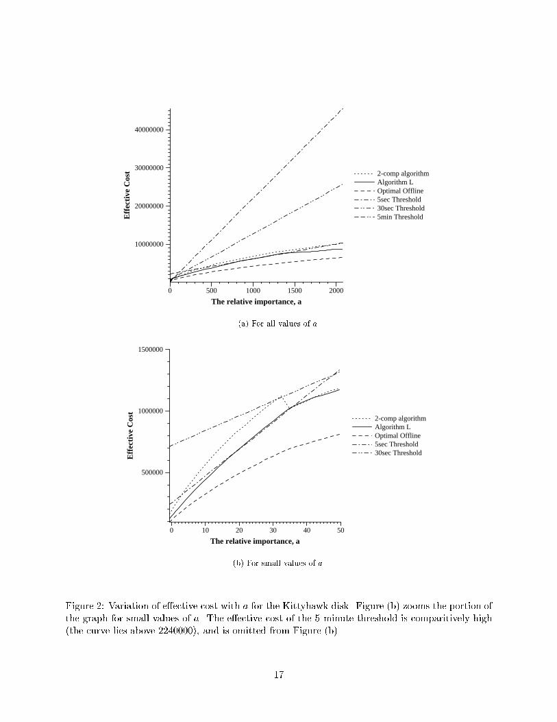
Characteristic Hewlett-PackardKittyhawk C3014A QuantumGo�Drive 120Capacity (Mbytes) 40 120Power consumed, active, (W) 1.50 1.65Power consumed, idle, (W) 0.62 1.00Power consumed, spundown (W) 0.27 0.20Power consumed, spinup (W) 2.17 5.50Normal time to spinup (s) 1.10 2.50Normal time to spindown (s) 0.55 6.00Avg time to read 1 Kbyte (ms) 22.50 26.7Table 1: Disk characteristics of the Kittyhawk C3014A and Quantum Go�Drive 120. (This tableappears in [DKM].)7.1 MethodologyWe simulated algorithm L using a disk access trace from a Hewlett-Packard 9000/845 personalworkstation running HP-UX. This trace is described in [RuW], and a portion of this trace was alsoused in a previous study of disk spindown policies [DKM]. The trace was obtained by Ruemmlerand Wilkes by monitoring the disk for roughly two months; it consisted of 416262 accesses to disk.We studied our algorithm for two disks, the Kittyhawk C3014A and the Quantum Go�Drive.The characteristics of the two drives are given in Table 1. (This table is derived from [DKM].) Forour studies, we merged the active and idle states of the disk into one active state; notice that adisk can read and write data only in the active state. By merging these two states we ensure thata \buy" corresponds to a spindown. As in [DKM], we assumed that a disk access takes the averagetime for seek and rotational latency. We also assumed that all operations and state transitionstake the average or \typical" time speci�ed by the manufacturer, if one is speci�ed, or else themaximum time.It is di�cult to determine from a disk access trace why a speci�c access arrived at disk. Weassumed that, if the disk is spundown, the application waits for the disk to spinup and complete therequested operation, and then performs the same sequence of operations as in the original system.In other words, although our simulations used disks that were di�erent from the one on which thetrace was collected, in our simulator we maintained the inter-arrival time of events at disk as in theoriginal trace: if, in the original trace, the tth access at disk arrived � seconds after the (t� 1)thaccess, in our simulation, we assumed that the tth access arrived � seconds after the (t � 1)thaccess was completed by the disk. The basic problem with any strategy is that data dependencybetween di�erent operations cannot be derived from the trace.We performed simulations for di�erent values of a, the relative importance of response time toenergy. For each a, we computed the buy cost c using the strategy described in Section 6. Wecompared our algorithm L against the following online algorithms: the two-competitive algorithm,which spins down the disk after c seconds of inactivity, and �xed-threshold policies that spindownthe disk after 5 seconds, 30 seconds, and 5 minutes of inactivity; we also compared algorithm Lagainst the optimal o�ine rent-to-buy algorithm, which knows the future and spins down thedisk immediately if the next access is to take place more than c seconds in the future. For eachalgorithm X, we computed EX , the excess energy consumed, OX , the number of operations delayedby a spinup; from these values we computed ECX , the e�ective cost of algorithm X, using (4).15

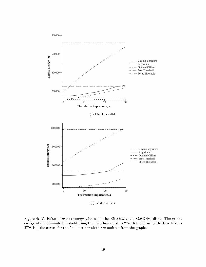
For the HP trace, the maximum inter-arrival time was 1770.4 seconds; the maximum a we usedcorresponded to a c of 1770.4.7.2 ResultsIn this section we present the results of our simulations. We �rst see how the e�ective cost varieswith parameter a, and then look at how excess energy and number of operations delayed varywith a. Recall that the parameter a is linearly related to the buy cost c. In particular, for theKittyhawk disk, c = 2:54 + a=1:225, and for the Go�Drive, c = 10:33 + a=1:45.The discussion from Section 6 implies that algorithm L and the 2-competitive algorithm try tooptimize for e�ective cost as de�ned by (4). In particular, for really small values of a, algorithm Lwill essentially try to reduce excess energy, and for really large values of a, algorithm L willessentially try to reduce number of operations delayed.7.2.1 E�ective Cost vs. aFigures 2 and 3 show how the e�ective cost varies with parameter a using the Kittyhawk andGo�Drive disks respectively. Each �gure plots the curves for all values of a, and a clearer view forwhen a is small.We observe that algorithm L performs best amongst the online algorithms for (almost) all valuesof a. (It is roughly 1% worse than the 5 second threshold for a lying between 18 and 34 while usingthe Kittyhawk disk, and for a lying between 14 and 28 while using the Go�Drive.) In particular, thee�ective cost for algorithm L is 6{25% less than the e�ective cost of the 2-competitive algorithm(except for a small range of values of a between 34 and 60 with the Kittyhawk disk and for abetween 28 and 58 for the Go�Drive when the e�ective costs for the two algorithms are roughlythe same).As should be expected, each �xed threshold algorithm performs well for a very limited rangeof values for a. Interestingly, the 5 second threshold for certain small values of a and the 5 minutethreshold for certain large values of a performs better than the 2-competitive algorithm.7.2.2 Excess Energy vs. aAs discussed in Section 6, when a is small, conserving energy is more important. Figure 4 plotsthe variation of excess energy with a using the Kittyhawk and Go�Drive disks for the variousalgorithms.We observe that for small values of a, algorithm L has the smallest excess energy amongstall online algorithms. In fact, it does better than the 5 second threshold, and its curve is almostparallel to the curve for the optimal o�ine algorithm. In particular, algorithm L saves 17{60%more excess energy as compared to the 2-competitive algorithm, and 6{42% more excess energy ascompared to the 5 second spindown threshold for small values of a (i.e., a < 25).We also observe that for small values of a, the 5 second threshold does better than the 2-competitive algorithm in terms of saving excess energy. (From Figures 2 and 3, we observe that formost of these values of a, the 5 second threshold is also better than the 2-competitive algorithm interms of e�ective cost.)16

0 500 1000 1500 2000

The relative importance, a

10000000

20000000

30000000

40000000E

ffec

tive

Cos

t 2-comp algorithmAlgorithm LOptimal Offline5sec Threshold30sec Threshold5min Threshold

(a) For all values of a.

0 10 20 30 40 50

The relative importance, a

500000

1000000

1500000

Eff

ecti

ve C

ost

2-comp algorithmAlgorithm LOptimal Offline5sec Threshold30sec Threshold

(b) For small values of a.Figure 2: Variation of e�ective cost with a for the Kittyhawk disk. Figure (b) zooms the portion ofthe graph for small values of a. The e�ective cost of the 5 minute threshold is comparitively high(the curve lies above 2240000), and is omitted from Figure (b).17

0 500 1000 1500 2000

The relative importance, a

10000000

20000000

30000000

40000000

50000000

Eff

ecti

ve C

ost 2-comp algorithm

Algorithm LOptimal Offline5sec Threshold30sec Threshold5min Threshold

(a) For all values of a.

0 50 100

The relative importance, a

500000

1000000

1500000

2000000

Eff

ecti

ve C

ost

2-comp algorithmAlgorithm LOptimal Offline5sec Threshold30sec Threshold

(b) For small values of a.Figure 3: Variation of e�ective cost with a for the Go�Drive disk. Figure (b) zooms the portionof the graph for small values of a. The e�ective cost of the 5 minute threshold is comparitivelyhigh (the curve lies above 2700000), and is omitted from Figure (b); similarly, the curves for the5 second and 30 second policies have been cropped at smaller values of a to show the details of theother three curves. 18

0 10 20 30

The relative importance, a

200000

400000

600000

800000

Exc

ess

Ene

rgy

(J)

2-comp algorithmAlgorithm LOptimal Offline5sec Threshold30sec Threshold

(a) Kittyhawk disk.

0 10 20 30

The relative importance, a

400000

600000

800000

1000000

Exc

ess

Ene

rgy

(J)

2-comp algorithmAlgorithm LOptimal Offline5sec Threshold30sec Threshold

(b) Go�Drive disk.Figure 4: Variation of excess energy with a for the Kittyhawk and Go�Drive disks. The excessenergy of the 5 minute threshold using the Kittyhawk disk is 2249 KJ, and using the Go�Drive is2708 KJ; the curves for the 5 minute threshold are omitted from the graphs.19

7.2.3 Operations Delayed vs. aAs discussed in Section 6, when a is large, we want to reduce the number of operations delayed.Figure 5 plots the variation of number of operations delayed with a using the Kittyhawk andGo�Drive disks for the various algorithms.We observe two interesting phenomenon: �rst, the curves for the 2-competitive algorithm andthe optimal o�ine algorithm coincide for a large range of values for a. Second, algorithm L reducesnumber of operations delayed over both these algorithms for su�ciently large a.7.2.4 Adaptability and Rent-to-BuyA di�erent way of viewing the tradeo� between excess energy and response time is presented inFigure 6. In this �gure, excess energy is plotted as a function of number of operations delayed,and the di�erent points on the curve are obtained by varying a; in particular, the value of a (orequivalently, c) decreases from left to right along the curve. (The curve for the Go�Drive is similarin shape and is omitted.)Figure 6 clearly shows the tradeo� between excess energy and response time obtained by vary-ing a. We observe that by increasing the value of one parameter a (equivalent to varying the valueof the buy cost c), we can e�ectively trade power for response time. Concerns on how to e�ectivelytrade power for response time have been raised for the disk spindown problem [DKB, DKM], andthe rent-to-buy model provides an elegant way of achieving this tradeo�.7.2.5 Other ObservationsSome other observations from our simulations are as follows:1. As mentioned in Section 7.2.2, energy conservation is crucial when a is small, and algorithm Lis best amongst the online algorithms in terms of excess energy for small a. Interestingly,we observed that the excess energy of algorithm L is less than the excess energy of the2-competitive algorithm for all values of a.2. We also compared our algorithm L against Ls allowing at most 25 potential cuto�s for al-gorithm Ls. Not surprisingly, algorithm L performed better than algorithm Ls; however,preliminary results suggest that algorithm L typically saved only 2{5% more excess energythan algorithm Ls. Allowing more potential cuto�s for algorithm Ls might help.3. In our simulations, we used at most 300 cuto�s for our algorithm L. The computation timefor the algorithm was therefore minimal. Interestingly, algorithm L did not change its cuto�stoo often in stage 2. (The cuto� changed between 14{56 times when measured over all valuesof a.)4. For measuring response time performance, we used the metric of the number of operationsdelayed. An alternative measure of response time performance is RX , the number of readoperations delayed by a spinup for algorithm X [DKM]. This metric rede�nes the e�ectivecost from (4) as E + a � RX . The rent-to-buy model can be easily modi�ed to evaluate thismeasure, by having di�erent costs for a spindown (i.e., di�erent c's) depending on whetherthe operation is a read or a write. We plan to consider the e�ect of this modi�cation to therent-to-buy cost in future work. 20

0 500 1000 1500 2000

The relative importance, a

10000

20000

30000

Num

ber

of o

pera

tion

s de

laye

d

2-comp algorithmAlgorithm LOptimal Offline5sec Threshold30sec Threshold5min Threshold

(a) Kittyhawk disk.

0 500 1000 1500 2000

The relative importance, a

5000

10000

15000

20000

25000

Num

ber

of O

pera

tion

s D

elay

ed

2-comp algorithmAlgorithm LOptimal Offline5sec Threshold30sec Threshold5min Threshold

(b) Go�Drive disk.Figure 5: Variation of the number of operations delayed with a for the Kittyhawk and Go�Drivedisks. The curves for the 2-competitive algorithm and the optimal o�ine algorithm coincide for alarge range of values of a.21

10000 20000 30000

Number of Operations Delayed

2000000

4000000

6000000

Exc

ess

Ene

rgy

(J)

Figure 6: Excess Energy, EL, as a function of the number of operations delayed, OL, for algorithm L.The graph was obtained by varying a (i.e., c); the value of a increases along the curve from left toright.

0 500 1000 1500 2000

The relative importance, a

2000

4000

6000

8000

10000

12000

Num

ber

of R

eads

del

ayed

2-comp algorithmAlgorithm LOptimal Offline5sec Threshold30sec Threshold5min Threshold

Figure 7: Number of reads delayed as a function of a for the various algorithms, while the rent-to-buy algorithms are optimizing using the de�nition of e�ective cost from (4). This graph is purelyfor illustration and comparison with Figure 5a. See Section 7.2.5, Item 4.For purely comparison purposes, Figure 7 plots the number of reads delayed as a function of afor the di�erent algorithms; the algorithms are still optimizing for e�ective cost as de�nedby (4). (In other words, the rent-to-buy algorithms think they are optimizing for number ofoperations delayed, while we measure the number of reads delayed.) Interestingly, the curves22

from Figure 7 are similar to the corresponding curves from Figure 5a, suggesting that weshould expect to obtain similar results as presented in this paper by using the number ofreads delayed metric instead of the number of operations delayed metric, when we modify thede�nition for e�ective cost appropriately.8 ConclusionsIn this paper we have looked at the problem of a sequence of unit rent-to-buy choices where theresource use times are independently drawn from an unknown probability distribution. We havelooked at computationally e�cient strategies whose expected cost for the tth resource use convergesto optimal as t!1 for any bounded probability distribution on the resource use times. We havealso looked at a �xed-space algorithm which almost converges to optimal. We are currently lookingat modeling the resource use times as being generated by a Hidden Markov Model (HMM) andhave optimality results for special types of HMMs. Recently, Markov models have been e�ectivelyused to analyze caching and prefetching algorithms assuming user requests to pages in cache aregenerated by Markov sources [KPR, KrV, ViK].Simulations of our algorithm for the disk spindown problem using disk access traces obtainedfrom HP suggest that the rent-to-buy model is a good way to study disk spindown and relatedsystems issues; in particular, a single parameter c e�ectively models the tradeo� between powerand response-time. We also introduced the new metric of \excess energy" that really re ects therelative performance in terms of energy consumed of one disk spindown algorithm against another.We introduced a natural notion of \e�ective cost" that incorporates the two metrics of excessenergy, and number of operations delayed weighted by a user speci�ed parameter a, into one cost.We observed that our algorithm L out-performed other online algorithms in terms of e�ective costfor almost all values of a; in particular, it had 6{25% less e�ective cost than the 2-competitivealgorithm. In addition, for small values of a (corresponding to when saving energy is critical), weobserved that our algorithm L saves 17{60% more of excess energy as compared to the 2-competitivealgorithm, and 6{42% more excess energy as compared to the 5 second �xed threshold.AcknowledgementsWe thank John Wilkes and Hewlett-Packard Company for making their �le system traces availableto us. We thank Peter Bartlett for his comments, and Fred Douglis for his comments and interestingdiscussions related to the disk spindown problem.References[BEH] A. Blumer, A. Ehrenfeucht, D. Haussler, and M. K. Warmuth, \Learnability and theVapnik Chervonenkis Dimension," Journal of the ACM (October 1989).[DKB] F. Douglis, P. Krishnan, and B. Bershad, \Adaptive Disk Spindown Policies for MobileComputers," Proceedings of the Second USENIX Symposium on Mobile and Location In-dependent Computing , to appear.23

[DKM] F. Douglis, P. Krishnan, and B. Marsh, \Thwarting the Power Hungry Disk," Proceedingsof the 1994 Winter USENIX Conference (January 1994).[Gre] P. Greenawalt, \Modeling Power Management for Hard Disks," Proceedings of the Sym-posium on Modeling and Simulation of Computer Telecommunication Systems (1994).[KLM] A. R. Karlin, K. Li, M. S. Manasse, and S. Owicki, \Empirical Studies of CompetitiveSpinning for a Shared-Memory Multiprocessor ," Proceedings of the 1991 ACM Symposiumon Operating System Principles (1991), 41{55.[KMM] A. R. Karlin, M. S. Manasse, L. A. McGeoch, and S. Owicki, \Competitive RandomizedAlgorithms for Non-Uniform Problems," Proceedings of the 1st ACM-SIAM Symposiumon Discrete Algorithms (1990), 301{309.[KPR] A. R. Karlin, S. J. Phillips, and P. Raghavan, \Markov Paging," Proceedings of the 33rdAnnual IEEE Conference on Foundations of Computer Science (October 1992), 208{217.[KeS] M. J. Kearns and R. E. Schapire, \E�cient Distribution-Free Learning of ProbabilisticConcepts," Proceedings of the 31st Annual IEEE Symposium on Foundations of ComputerScience (October 1990), 382{391.[KLP] S. Keshav, C. Lund, S. J. Phillips, N. Reingold, and H. Saran, \An Empirical Evalua-tion of Virtual Circuit Holding Time Policies in IP-over-ATM Networks," Proceedings ofINFOCOM '95 .[KrV] P. Krishnan and J. S. Vitter, \Optimal Prediction for Prefetching in the Worst Case,"Proceedings of the Fifth Annual ACM-SIAM Symposium on Discrete Algorithms (January1994), Also appears as Duke University Technical Report CS-1993-26..[LKH] K. Li, R. Kumpf, P. Horton, and T. Anderson, \A Quantitative Analysis of Disk DrivePower Management in Portable Computers," Proceedings of the 1994 Winter USENIX(January 1994).[LPR] C. Lund, S. Phillips, and N. Reingold, \IP over Connection-Oriented Networks and Dis-tributed Paging," Proceedings of the 35th Annual IEEE Symposium on Foundations ofComputer Science (November 1994), 424{434.[MDK] B. Marsh, F. Douglis, and P. Krishnan, \Flash Memory File Caching for Mobile Com-puters," Proceedings of the 27th IEEE Hawaii Conference on System Sciences (January1994).[Pac] Hewlett Packard, \Kittyhawk HP C3013A/C3014A Personal Storage Modules TechnicalReference Manual," March 1993, HP Part No. 5961-4343.[Pol] D. Pollard, Convergence of Stochastic Processes, Springer-Verlag, 1984.[RuW] C. Ruemmler and J. Wilkes, \UNIX Disk Access Patterns," Proceedings of the 1993 WinterUSENIX Conference (January 1993), 405{420.[SaK] H. Saran and S. Keshav, \An Empirical Evaluation of Virtual Circuit Holding Times inIP-over-ATM networks," Proceedings of INFOCOM '94 (June 1994).[Vap] V. N. Vapnik, \Inductive principles of the search for empirical dependences (methodsbased on weak convergence of probability measures)," Proceedings of the 1989 Workshopon Computational Learning Theory (1989).24

[VaC] V. N. Vapnik and A. Y. Chervonenkis, \On the Uniform Convergence of Relative Fre-quencies of Events to their Probabilities," Theoretical Probability and Its Applications 16(1971), 264{280.[ViK] J. S. Vitter and P. Krishnan, \Optimal Prefetching via Data Compression," Proceedings ofthe 32nd Annual IEEE Symposium on Foundations of Computer Science (October 1991),121{130, Also appears as Brown University Technical Report No. CS{91{46.

25